Concurrent Programming in Erlan Part 1

Note to readers:
This manuscript contains the complete text of Part I of Concurrent
programming in Erlang (ISBN 0-13-508301-X).
Prentice Hall has given us permission to make the text available.
Note that since Part II of the text (Applications) is missing all references
to pages and sections in Part II of the book are invalid and have been
replaced by question marks \??".
A free version of Erlang can be obtained from
http://www.ericsson.com/technology/opensource/erlang

This page is intentionally plank.

Concurrent Programming

in ERLANG

Second Edition

Joe Armstrong

Robert Virding

Claes Wikstr¨

Mike Williams

Ericsson

Telecommunications Systems Laboratories

Box 1505

S - 125 25 ¨

Alvsj¨

Sweden

PRENTICE HALL

Englewood Cliffs, New Jersey 07632

Contents

Preface

viii

Acknowledgments

Introduction

Programming

1 An ERLANG Tutorial

1.1

Sequential Programming

1.2

Data Types

1.3

Pattern Matching

1.4

Built-in Functions

1.5

Concurrency

2 Sequential Programming

2.1

Terms

2.2

Pattern Matching

2.3

Expression Evaluation

2.4

The Module System

2.5

Function Definition

2.6

Primitives

2.7

Arithmetic Expressions

2.8

Scope of Variables

3 Programming with Lists

3.1

List Processing BIFs

Contents

3.2

Some Common List Processing Functions

3.3

Examples

3.4

Common Patterns of Recursion on Lists

3.5

Functional Arguments

4 Programming with Tuples

4.1

Tuple Processing BIFs

4.2

Multiple Return Values

4.3

Encrypting PIN Codes

4.4

Dictionaries

4.5

Unbalanced Binary Trees

4.6

Balanced Binary Trees

5 Concurrent Programming

5.1

Process Creation

5.2

Inter-process Communication

5.3

Timeouts

5.4

Registered Processes

5.5

Client–Server Model

5.6

Process Scheduling, Real-time and Priorities

5.7

Process Groups

6 Distributed Programming

6.1

Motivation

6.2

Distributed mechanisms

6.3

Registered Processes

6.4

Connections

6.5

A Banking Example

7 Error Handling

7.1

Catch and Throw

7.2

Process Termination

7.3

Linked Processes

7.4

Run-time Failure

100

7.5

Changing the Default Signal Reception Action

102

7.6

Undefined Functions and Unregistered Names

106

7.7

Catch Versus Trapping Exits

108

8 Programming Robust Applications

109

8.1

Guarding Against Bad Data

109

8.2

Robust Server Processes

111

8.3

Isolating Computations

114

8.4

Keeping Processes Alive

115

8.5

Discussion

115

Contents

vii

9 Miscellaneous Items

118

9.1

Last Call Optimisation

118

9.2

References

121

9.3

Code Replacement

121

9.4

Ports

123

9.5

Binaries

130

9.6

Process Dictionary

132

9.7

The Net Kernel

133

9.8

Hashing

136

9.9

Efficiency

138

Applications

141

Bibliography

143

A ERLANG Reference Grammar

145

B Built-in Functions

150

B.1

The BIFs

151

B.2

BIFs Sorted by Type

172

C The Standard Libraries

176

C.1

176

C.2

file

177

C.3

lists

178

C.4

code

179

D Errors in ERLANG

180

D.1

Match Errors

180

D.2

Throws

181

D.3

Exit signals

181

D.4

Undefined Functions

182

D.5

The error logger

182

E Drivers

183

Index

188

Preface

Erlang

is a declarative language for programming concurrent and distributed

systems which was developed by the authors at the Ericsson and Ellemtel Computer
Science Laboratories.

The development of Erlang started as an investigation into whether modern

declarative programming paradigms could be used for programming large industrial
telecommunications switching systems. It was soon realised that languages which
were suitable for programming telecommunications systems were also suitable for
a wide range of industrial embedded real-time control problems.

Many of the Erlang primitives provide solutions to problems which are com-

monly encountered when programming large concurrent real-time systems. The
module system allows the structuring of very large programs into conceptually
manageable units. Error detection mechanisms allow the construction of fault-
tolerant software. Code loading primitives allow code in a running system to be
changed without stopping the system.

Erlang

has a process-based model of concurrency. Concurrency is explicit

and the user can precisely control which computations are performed sequentially
and which are performed in parallel. Message passing between processes is asyn-
chronous, that is, the sending process continues as soon as a message has been
sent.

The only method by which Erlang processes can exchange data is message

passing. This results in applications which can easily be distributed – an applica-
tion written for a uniprocessor can easily be changed to run on a multiprocessor
or network of uniprocessors. The language has built-in mechanisms for distributed
programming which makes it easy to write applications which can run either on a

Agner Krarup Erlang (1878–1929) was a Danish mathematician who developed a theory of

stochastic processes in statistical equilibrium – his theories are widely used in the telecommuni-
cations industry.

This is very important in embedded real-time systems such as telephone exchanges or air

traffic control systems – such systems should not normally be stopped for software maintenance
purposes.

viii

single computer, or on a network of computers.

Variables in Erlang have the property of single assignment

– once a value has

been assigned to a variable this value can never be changed. This property has
important consequences when debugging or transforming a program.

Programs are written entirely in terms of functions – function selection is made

by pattern matching which leads to highly succinct programs.

The Erlang system has an inbuilt notion of time – the programmer can specify

how long a process should wait for a message before taking some action. This
allows the programming of real-time applications. Erlang is suitable for most
soft real-time applications where response times are in the order of milliseconds.

Current information about Erlang can be obtained from the World Wide Web

at http://www.ericsson.se/erlang, e-mail requests for information can be sent
to erlang@erix.ericsson.se.

Commercially supported implementations of Erlang can be obtained from

Ericsson Software Technology AB. For information please send e-mail to
erl-biz@erlang.ericsson.se.

Joe Armstrong

Robert Virding

Claes Wikstr¨

Mike Williams

Computer Science Laboratory

Ericsson Telecommunications Systems Laboratories

Box 1505

S-125 25 ¨

Alvsj¨

Sweden

erlang@erix.ericsson.se

Also called write-once variables or non-destructive assignment.

Acknowledgments

The ideas in Erlang are difficult to trace to a single source. Many features of the
language have been influenced and improved as a result of comments by our friends
and colleagues of the Computer Science Laboratory and we would like to thank
them all for their help and advice. In particular we would like to thank Bjarne
D¨

acker – Head of the Computer Science Laboratory – for his enthusiastic support

and encouragement and for the help he has provided in spreading the language.

Many people have made contributions to this book. Richard Ehrenborg wrote

the code for AVL trees in Chapter ??. Per Hedeland wrote pxw which is described
in Chapter ??. Roger Skagervall and Sebastian Strollo provided the ideas behind
the object-oriented programming methods described in Chapter ??. Carl Wilhelm
Welin wrote an LALR(1) parser generator in Erlang which generates Erlang
and provided the reference grammar contained in Appendix A.

Early users, in particular the first group of users (ingen n¨

amnd, ingen gl¨

omd)

at Ericsson Business Systems in Bollmora stoically acted as guinea pigs and did
battle with many early and mutually incompatible versions of the Erlang system.
Their comments have helped us greatly.

We would like to thank Torbj¨

orn Johnson from Ellemtel and Bernt Ericson from

Ericsson Telecom without whose unfailing support Erlang would not have seen
the light of day.

This book was typeset in LaTEX with the macro package ph.sty provided by

Richard Fidczuk from Prentice Hall. Comp.text.tex also helped answer our na¨ıve
questions.

‘UNIX’ is a registered trademark of AT&T, Bell Laboratories. ‘X Window Sys-

tem’ is a trademark of MIT.

Introduction

Erlang

is a new programming language which was designed for programming

concurrent, real-time, distributed fault-tolerant systems.

Programming techniques for programming concurrent real-time systems have,

for many years, lagged behind those techniques used for programming sequential
applications. When the use of languages such as C or Pascal was standard practice
for programming sequential applications, most programmers of real-time systems
were still struggling with assembly languages. Today’s real-time systems can be
written in languages such as Ada, Modula2, Occam, etc., in which there are explicit
constructs for programming concurrency or in languages such as C which lack
constructs for concurrency.

Our interest in concurrency is motivated by a study of problems which exhibit a

large degree of natural concurrency. This is a typical property of real-time control
problems. The Erlang programmer explicitly specifies which activities are to be
represented as parallel processes. This view of concurrency is similar to that found
in Occam, CSP, Concurrent Pascal, etc., but dissimilar to concurrent languages
where the prime motivation for introducing concurrency is not for modelling real
world concurrency, but for obtaining higher performance by compiling programs
for execution on a parallel processor.

Languages such as Prolog [?] and ML [?] are now used for a wide range of

industrial applications and have resulted in dramatic reductions in the total effort
required to design, implement and maintain applications. We have designed and
implemented Erlang to enable the programming of concurrent real-time systems
at a similarly high level.

Declarative syntax. Erlang has a declarative syntax and is largely free from

side-effects.

Concurrent. Erlang has a process-based model of concurrency with asynchron-

ous message passing. The concurrency mechanisms in Erlang are light-
weight, i.e. processes require little memory, and creating and deleting pro-
cesses and message passing require little computational effort.

Introduction

Real-time. Erlang is intended for programming soft real-time systems where

response times in the order of milliseconds are required.

Continuous operation. Erlang has primitives which allow code to be replaced

in a running system and allow old and new versions of code to execute at the
same time. This is of great use in ‘non-stop’ systems, telephone exchanges,
air traffic control systems, etc., where the systems cannot be halted to make
changes in the software.

Robust. Safety is a crucial requirement in systems such as the above. There are

three constructs in the language for detecting run-time errors. These can be
used to program robust applications.

Memory management. Erlang is a symbolic programming language with a

real-time garbage collector.

Memory is allocated automatically when re-

quired, and deallocated when no longer used. Typical programming errors
associated with memory management cannot occur.

Distribution. Erlang has no shared memory. All interaction between processes

is by asynchronous message passing. Distributed systems can easily be built
in Erlang. Applications written for a single processor can, without diffi-
culty, be ported to run on networks of processors.

Integration. Erlang can easily call or make use of programs written in other

programming languages. These can be interfaced to the system in such a
way that they appear to the programmer as if they were written in Erlang.

We have freely borrowed ideas from declarative and concurrent programming

languages. The early syntax of Erlang owed much to STRAND [?], though the
current syntax is more reminiscent of an untyped ML. The model of concurrency
is similar to that of SDL [?].

Our goal was to produce a small, simple and efficient language suitable for pro-

gramming robust large-scale concurrent industrial applications. Thus, for reasons
of efficiency, we have avoided many features commonly found in modern functional
or logic programming languages. Currying, higher-order functions, lazy evalua-
tion, ZF comprehension, logical variables, deep guards, etc., add to the expressive
power of a declarative programming language, but their absence is not a significant
detriment to the programming of typical industrial control applications. The use
of a pattern matching syntax, and the ‘single assignment’ property of Erlang
variables, leads to clear, short and reliable programs.

Erlang

was designed at the same time as its first implementation, which was an

interpreter written in Prolog [?]. We were fortunate in having an enthusiastic group
of users who were, at the same time, developing a prototype of a new telephone
exchange.

This resulted in an extremely pragmatic approach to language design. Con-

structs which were not used were removed. New constructs were introduced to
solve problems which had caused our users to write convoluted code. Despite the
fact that we often introduced backwardly incompatible changes to the language,
our users had soon produced tens of thousands of lines of code and were actively

Introduction

encouraging others to use the language. Some of the results of their labours in
producing a new way of programming telephone exchanges have been published in
[?], [?].

The first Prolog-based interpreter for Erlang has long since been abandoned

in favour of compiled implementations. One of these implementations is available
free of charge but is subject to non-commercial licensing. The present generation
of Erlang implementations meets our real-time requirements as regards speed
and lightweight concurrency. Erlang implementations have been ported to and
run on several operating systems and several processors.

Erlang

is suitable for programming a wide range of concurrent applications.

Several tools have been written to support Erlang programming, for example,
interfaces to the X Windows System, and ASN.1 compiler (written in Erlang and
generating Erlang), parser generators, debuggers . . .

Audience

This book is intended for people who are interested in real-time control systems and
have some previous programming experience. Previous knowledge of functional or
logic languages is not necessary.

The material in the book is loosely based on an Erlang course which has been

held many times in recent years at Ericsson and its subsidiary companies world-
wide and at several Swedish universities. This course takes four days, which is more
than sufficient to teach not only the language but also many of the paradigms used
in Erlang programming. The last day of the course usually has a programming
exercise in which the students write a control system for a telephone exchange
similar to that described in Chapter ?? and run it on a real exchange!

Summary

The book is divided into two main parts. The first part, ‘Programming’, introduces
the Erlang language and some of the most commonly used paradigms when
programming in Erlang. The second part, ‘Applications’, has a number of self-
contained chapters containing case studies of typical Erlang applications.

Programming

Chapter ?? is a tutorial introduction to Erlang. The major ideas in the language
are introduced through a series of examples.

Chapter ?? introduces sequential programming. The module system is intro-

duced, as is the basic terminology used when we talk about Erlang programs.

Introduction

Chapters ?? and ?? contain examples of sequential programming with lists and

tuples. Basic list and tuple programming techniques are introduced. Several stand-
ard modules, which will be used later in the book, are introduced. These include
modules for implementing sets, dictionaries, balanced and unbalanced binary trees,
etc.

Chapter ?? introduces concurrency. Sequential Erlang needs the addition of

a small number of primitives to turn it into a concurrent programming language.
We introduce the primitives necessary to create a parallel process and for message
passing between processes. We also introduce the idea of a registered process which
allows us to associate a name with a process.

The basic ideas behind the client–server model are explained. This model is

often used in later chapters and is one of the basic programming techniques for
coordinating the activities of several parallel processes. We also introduce timeouts,
which can be used for writing programs which have real-time behaviour.

Chapter ?? has a general introduction to distributed programming where we

explain some of the reasons for writing distributed applications. We describe the
language primitives which are needed to write distributed Erlang programs and
explain how sets of Erlang process can be arranged to run on a network of

Erlang

nodes.

Chapter ?? explains the error handling mechanisms available in Erlang. We

have designed Erlang for programming robust applications, and the language
has three orthogonal mechanisms for detecting errors. We take the view that
the language should detect as many errors as possible at run-time and leave the
responsibility for correction of such errors to the programmer.

Chapter ?? shows how the error handling primitives introduced in the previous

chapter can be used to build robust and fault-tolerant systems. We show how to
protect against faulty code, provide a fault-tolerant server (by extending the client
server model) and show how to ‘isolate’ a computation so as to limit the extent of
any damage caused if it should fail.

Chapter ?? is a collection of ideas and programming techniques not introduced

elsewhere in the book. We start with a discussion of the last call optimisation. An
understanding of this optimisation is essential if the programmer wishes to write
correct code for non-terminating software. We then introduce references which
provide unique unforgeable symbols. The next two sections in this chapter contain
details of how to change Erlang code in a running system (this is needed for
writing non-stop systems) and how to interface Erlang to programs written in
other languages. Following this we discuss binaries which are used for efficiently
handling large quantities of untyped data, the process dictionary which provides
each process with simple destructive storage capabilities and the net kernel which
is the basis of distributed Erlang. Finally, we discuss efficiency, giving examples
of how to write efficient Erlang code.

Introduction

Applications

Chapter ?? shows how to program databases in Erlang. We start by combining
the simple dictionary module developed in Chapter ??

with the client–server

model of Chapter ??. This gives a simple concurrent database. We then show
how to increase throughput in the database by representing it as a multi-level tree
of parallel processes. We then add the notion of a transaction whereby several
sequential operations on the database can be made to appear atomic.

Following this, we add roll-back to the database which allows us to ‘undo’ the

effect of a transaction. The roll-back example provides a beautiful instance of the
use of non-destructive assignment.

We discuss how our database can be made fault-tolerant. Finally, we show how

an external database can be integrated with our database in such a way that the
entire system presents a consistent interface to the programmer.

Chapter ??

introduces distributed programming techniques.

We show how

several well-known techniques used for writing distributed programs, such as the
remote proceedure call, broadcasting, promises, etc. can be programmed in dis-
tributed Erlang.

Chapter ?? examines the problem of distributed data. Many applications run-

ning on different physical machines may wish to share some comon data structures.
This chapter describes various techniques which can be used for implementing
shared data in a distributed system.

Chapter ?? is a discussion of the Erlang operating system. Since all process

management occurs within Erlang we need few of the services of a traditional
operating system. We show the main components of the Erlang operating sys-
tem which accompanies the standard distribution of the language. This operating
system can be used as the basis of more specialised operating systems which may
be required for a specific turn-key application.

Chapter ?? address two real-time control problems. The first is the well-known

problem of controlling a number of lifts – here we see that modelling the system as a
set of parallel processes provides a simple and elegant solution. The second section
addresses ‘process control’ – in this case our ‘process’ is a satellite. The only way
of ‘observing’ the satellite is by interpreting the data which comes from sensors
mounted in the satellite. The only way of modifying the behaviour of the satellite
is by sending commands to instruments on the satellite. While we have chosen a
satellite control system in our example, the techniques are equally applicable to a
wide range of control problems.

Chapter ?? is a complete example of a real-time control program for a small local

telephone exchange. Erlang was developed at the Ericsson Computer Science
Laboratory and Ericsson is one of the world’s major manufacturers of telephone
exchanges – ease of programming telephony has always been (and still is) one of
our principal interests!

The example in the chapter is only a ‘toy’ example. It is, however, fully func-

tional and illustrates many of the techniques used in building telephony software in

Introduction

Erlang

. The example given is the baby brother of much larger Erlang programs

which have been developed for controlling complex telephony applications. These
programs run into tens of thousands of lines of Erlang code and are extensions
of the programming techniques described in this chapter.

The chapter ends with a short introduction to SDL (SDL is widely used to

specify the behaviour of telecommunication systems) – we show the one-to-one
correspondence between a part of an SDL specification and the Erlang code
which is an implementation of the specification. The conceptual ‘gap’ between the
SDL and the Erlang code is small – a factor which can be used to reduce the
cost of designing and implementing a real-time system.

Chapter ?? has a short introduction to ASN.1 and presents a cross-compiler

from ASN.1 to Erlang. ASN.1 is standard for describing data formats used
in communication protocols. The chapter shows the similarity between ASN.1
specifications and Erlang code which could be used to manipulate data packets
described in ASN.1. The ability to generate code automatically for large parts of
the communication software of a system greatly simplifies the construction of the
system.

Chapter ?? shows how to build a graphic user interface to an Erlang applica-

tion. The chapter illustrates two points: firstly, how a set of concurrent processes
maps nicely onto a set of objects in a windowing system; and secondly, the use of

Erlang

together with a large package written in a ‘foreign language’.

Chapter ?? we discuss some of the major properties of object-oriented program-

ming languages and how these can be programmed in Erlang. We discuss the
relation between an object-oriented design and an Erlang implementation of the
design.

Part I

Programming

Chapter 1

An ERLANG Tutorial

We begin with a tutorial introduction to Erlang. Our intention is to introduce
the reader to the main features of the language. Many of the topics covered will
not be explained in detail here, but will be discussed in subsequent chapters of the
book.

We start with examples of simple sequential Erlang programs.

1.1

Sequential Programming

Program 1.1 computes the factorial of an integer.

-module(math1).
-export([factorial/1]).

factorial(0) -> 1;
factorial(N) -> N * factorial(N-1).

Program 1.1

Functions can be interactively evaluated using a program called the shell. The

shell prompts for an expression and then evaluates and prints any expression which
the user enters, for example:

> math1:factorial(6).
720
> math1:factorial(25).
15511210043330985984000000

In the above ‘>’ is the shell prompt. The remainder of the line is the expression

entered by the user. The following line is the result of the expression evaluation.

An ERLANG Tutorial

How the code for factorial was compiled and loaded into the Erlang system

is a local issue.

In our example, the function factorial has two defining clauses: the first

clause is a rule for computing factorial(0), the second a rule for computing
factorial(N). When evaluating factorial for some argument, the two clauses
are scanned sequentially, in the order in which they occur in the module, until one
of them matches the call. When a match occurs, the expression on the right-hand
side of the ‘->’ symbol is evaluated, and any variables occurring in the function
definition are substituted in the right-hand side of the clause before it is evaluated.

All Erlang functions belong to some particular module. The simplest possible

module contains a module declaration, export declarations and code representing
the functions which are exported from the module.

Exported functions can be run from outside the module. All other functions can

only be run from within the module.

Program 1.2 gives an example of this.

-module(math2).
-export([double/1]).

double(X) ->

times(X, 2).

times(X, N) ->

X * N.

Program 1.2

The function double/1

can be evaluated from outside the module, whereas

times/2 is purely local, for example:

> math2:double(10).
20
> math2:times(5, 2).
** undefined function: math2:times(5,2) **

In Program 1.2 the module declaration -module(math2) defines the name of the

module, and the export attribute -export([double/1]) says that the function
double with one argument is to be exported from the module.

By ‘local issue’ we mean that the details of how a particular operation is performed is system-

dependent and is not covered in this book.

The notation F/N denotes the function F with N arguments.

Sequential Programming

Function calls can be nested:

> math2:double(math2:double(2)).
8

Choice in Erlang is provided by pattern matching.

Program 1.3 gives an

example of this.

-module(math3).
-export([area/1]).

area({square, Side}) ->

Side * Side;

area({rectangle, X, Y}) ->

X * Y;

area({circle, Radius}) ->

3.14159 * Radius * Radius;

area({triangle, A, B, C}) ->

S = (A + B + C)/2,
math:sqrt(S*(S-A)*(S-B)*(S-C)).

Program 1.3

Evaluating math3:area({triangle, 3, 4, 5}) yields 6.0000 and

math3:area({square, 5}) yields 25 as expected. Program 1.3 introduces several
new ideas:

• Tuples – these are used as place holders for complex data structures. We can

illustrate this by the following dialogue with the shell:

> Thing = {triangle, 6, 7, 8}.
{triangle,6,7,8}
> math3:area(Thing).
20.3332

Here Thing is bound to the tuple {triangle, 6, 7, 8} – we say the value
of Thing is a tuple of size 4 – it has four elements. The first element is the
atom triangle, and the next three elements are the integers 6, 7 and 8.

• Pattern matching – this is used for clause selection within a function. area/1

was defined in terms of four clauses. The query math3:area({circle, 10})
results in the system trying to match one of the clauses defining area/1
with the tuple {circle, 10}. In our example the third clause representing
area/1 would match, and the free variable Radius occurring in the head of
the function definition is bound to the value supplied in the call (in this case
to 10).

An ERLANG Tutorial

• Sequences and temporary variables – these were introduced in the last clause

defining area/1. The body of the last clause is a sequence of two statements,
separated by a comma; these statements are evaluated sequentially. The
value of the clause is defined as the result of evaluating the last statement
in the sequence.

In the first statement of the sequence we introduced a

temporary variable S.

1.2

Data Types

Erlang

provides the following data types:

• Constant data types – these are data types which cannot be split into more

primitive subtypes:

– Numbers – for example: 123, -789, 3.14159, 7.8e12, -1.2e-45.

Numbers are further subdivided into integers and floats.

– Atoms – for example: abc, ’An atom with spaces’, monday, green,

hello_world. These are simply constants with names.

• Compound data types – these are used to group together other data types.

There are two compound data types:

– Tuples – for example: {a, 12, b}, {}, {1, 2, 3}, {a, b, c, d, e}.

Tuples are used for storing a fixed number of items and are written
as sequences of items enclosed in curly brackets. Tuples are similar to
records or structures in conventional programming languages.

– Lists – for example: [], [a, b, 12], [22], [a, ’hello friend’].

Lists are used for storing a variable number of items and are written as
sequences of items enclosed in square brackets.

Components of tuples and lists can themselves be any Erlang data item – this

allows us to create arbitrary complex structures.

The values of Erlang data types can be stored in variables. Variables always

start with an upper-case letter so, for example, the code fragment:

X = {book, preface, acknowledgments, contents,

{chapters, [

{chapter, 1, ’An Erlang Tutorial’},
{chapter, 2, ...}
]

}},

creates a complex data structure and stores it in the variable X.

Pattern Matching

1.3

Pattern Matching

Pattern matching is used for assigning values to variables and for controlling the
flow of a program. Erlang is a single assignment language, which means that
once a variable has been assigned a value, the value can never be changed.

Pattern matching is used to match patterns with terms. If a pattern and term

have the same shape then the match will succeed and any variables occurring in
the pattern will be bound to the data structures which occur in the corresponding
positions in the term.

1.3.1

Pattern matching when calling a function

Program 1.4 defines the function convert which is used to convert temperatures be-
tween the Celsius, Fahrenheit and R´

eaumur scales. The first argument to convert

is a tuple containing the scale and value of the temperature to be converted and
the second argument is the scale to which we wish to convert.

-module(temp).
-export([convert/2]).

convert({fahrenheit, Temp}, celsius) ->

{celsius, 5 * (Temp - 32) / 9};

convert({celsius, Temp}, fahrenheit) ->

{farenheit, 32 + Temp * 9 / 5};

convert({reaumur, Temp}, celsius) ->

{celsius, 10 * Temp / 8};

convert({celsius, Temp}, reaumur) ->

{reaumur, 8 * Temp / 10};

convert({X, _}, Y) ->

{cannot,convert,X,to,Y}.

Program 1.4

When convert is evaluated, the arguments occurring in the function call (terms)

are matched against the patterns occurring in the function definition. When a
match occurs the code following the ‘->’ symbol is evaluated, so:

> temp:convert({fahrenheit, 98.6}, celsius).
{celsius,37.0000}
> temp:convert({reaumur, 80}, celsius).
{celsius,100.000}
> temp:convert({reaumur, 80}, fahrenheit).
{cannot,convert,reaumur,to,fahrenheit}

An ERLANG Tutorial

1.3.2

The match primitive ‘=’

The expression Pattern = Expression causes Expression to be evaluated and
the result matched against Pattern. The match either succeeds or fails. If the
match succeeds any variables occurring in Pattern become bound, for example:

> N = {12, banana}.
{12,banana}
> {A, B} = N.
{12,banana}
> A.
12
> B.
banana

The match primitive can be used to unpack items from complex data structures:

> {A, B} = {[1,2,3], {x,y}}.
{[1,2,3],{x,y}}
> A.
[1,2,3]
> B.
{x,y}
> [a,X,b,Y] = [a,{hello, fred},b,1].
[a,{hello,fred},b,1]
> X.
{hello,fred}
> Y.
1
> {_,L,_} = {fred,{likes, [wine, women, song]},

{drinks, [whisky, beer]}}.

{fred,{likes,[wine,women,song]},{drinks,[whisky,beer]}}
> L.
{likes,[wine,women,song]}

The special variable underscore (written ‘_’) is the anonymous or don’t care

variable. It is used as a place holder where the syntax requires a variable, but the
value of the variable is of no interest.

If the match succeeds, the value of the expression Lhs = Rhs is defined to be

Rhs. This allows multiple uses of match within a single expression, for example:

{A, B} = {X, Y} = C = g(a, 12)

‘=’ is regarded as an infix right associative operator; thus A = B = C = D is parsed
as A = (B = (C = D)).

Built-in Functions

1.4

Built-in Functions

Some operations are impossible to program in Erlang itself, or are impossible to
program efficiently. For example, there is no way to find out the internal structure
of an atom, or the time of day, etc. – these lie outside the scope of the language.

Erlang

therefore has a number of built-in functions (BIFs) which perform these

operations.

For example atom_to_list/1 converts an atom to a list of (ASCII) integers

which represents the atom and date/0 returns the current date:

> atom_to_list(abc).
[97,98,99]
> date()
{93,1,10}

A full list of all BIFs is given in Appendix ??.

1.5

Concurrency

Erlang

is a concurrent programming language – this means that parallel activities

(processes) can be programmed directly in Erlang and that the parallelism is
provided by Erlang and not the host operating system.

In order to control a set of parallel activities Erlang has primitives for multi-

processing: spawn starts a parallel computation (called a process); send sends a
message to a process; and receive receives a message from a process.

spawn/3 starts execution of a parallel process and returns an identifier which

may be used to send messages to and receive messages from the process.

The syntax Pid ! Msg is used to send a message. Pid is an expression or constant

which must evaluate to a process identity. Msg is the message which is to be sent
to Pid. For example:

Pid ! {a, 12}

means send the message {a, 12} to the process with identifier Pid (Pid is short
for process identifier). All arguments are evaluated before sending the message,
so:

foo(12) ! math3:area({square, 5})

means evaluate the function foo(12) (this must yield a valid process identifier) and
evaluate math3:area({square, 5}) then send the result (i.e. 25) as a message
to the process. The order of evaluation of the two sides of the send primitive is
undefined.

The primitive receive is used to receive messages. receive has the following

syntax:

An ERLANG Tutorial

receive

Message1 ->

... ;

Message2 ->

... ;
...

end

This means try to receive a message which is described by one of the patterns

Message1,Message2,... The process which is evaluating this primitive is sus-
pended until a message which matches one of the patterns Message1,Message2,...
is received. If a match occurs the code after the ‘->’ is evaluated.

Any unbound variables occurring in the message reception patterns become

bound if a message is received.

The return value of receive is the value of the sequence which is evaluated as

a result of a receive option being matched.

While we can think of send as sending a message and receive as receiving a

message, a more accurate description would be to say that send sends a message
to the mailbox of a process and that receive tries to remove a message from the
mailbox of the current process.

receive is selective, that is to say, it takes the first message which matches

one of the message patterns from a queue of messages waiting for the attention of
the receiving process. If none of the receive patterns matches then the process is
suspended until the next message is received – unmatched messages are saved for
later processing.

1.5.1

An echo process

As a simple example of a concurrent process we will create an echo process which
echoes any message sent to it. Let us suppose that process A sends the message
{A, Msg} to the echo process, so that the echo process sends a new message con-
taining Msg back to process A. This is illustrated in Figure 1.1.

{A, Msg}

Msg

Figure 1.1 An echo process

Concurrency

In Program 1.5 echo:start() creates a simple echo process which returns any

message sent to it.

-module(echo).
-export([start/0, loop/0]).

start() ->

spawn(echo, loop, []).

loop() ->

receive

{From, Message} ->

From ! Message,
loop()

end.

Program 1.5

spawn(echo, loop, []) causes the function represented by echo:loop() to be

evaluated in parallel with the calling function. Thus evaluating:

...
Id = echo:start(),
Id ! {self(), hello}
...

causes a parallel process to be started and the message {self(), hello} to be
sent to the process – self() is a BIF which returns the process identifier of the
current process.

Chapter 2

Sequential Programming

This chapter introduces the concepts needed to write sequential Erlang programs.
We start with a discussion of the basic mechanisms by which variables acquire
values and how flow of control is achieved. To do this requires an understanding
of terms, patterns and pattern matching:

2.1

Terms

Erlang

provides the following data types

which are called terms:

• Constant data types

– Numbers

∗ Integers, for storing natural numbers
∗ Floats, for storing real numbers

– Atoms

– Pids (short for ‘process identifiers’), for storing process names

– References, for storing system unique references

• Compound data types

– Tuples, for storing a fixed number of terms

– Lists, for storing a variable number of terms

2.1.1

Numbers

Numbers are written as in the following examples:

Appendix A gives the formal Erlang grammar.

Terms

123 -34567 12.345 -27.45e-05

The precision of integers is a local issue but at least 24-bit integer precision must
be provided by any Erlang system.

The notation $<Char> represents the ASCII value of the character Char so, for

example, $A represents the integer 65.

Integers with base other than 10 are written using the notation <Base>#<Value>

so, for example, 16#ffff represents the integer 65535 (in base 10). The value of
Base must be an integer in the range 2..16.

Floating point numbers are written in conventional notation.

2.1.2

Atoms

Atoms are constants with names; thus, for example, the atoms monday, tuesday,
... could be used to represent days of the week in some program which performs
calendar calculations. Atoms are used to enhance the legibility of programs.

Examples of atoms:

friday

unquoted_atoms_cannot_contain_blanks

’A quoted atom which contains several blanks’
’hello \n my friend’

Atoms begin with a lower-case letter (a..z) and are terminated by a non-

alphanumeric character – otherwise they must be quoted.

By enclosing the atom name in single quotes any character may be included

within the atom. Atoms will always be printed in such a manner that they can be
read back by the Erlang reader. Within a quoted atom the following conventions
apply:

Characters

Meaning

backspace

delete

escape

form feed

newline

carriage return

tab

vertical tab

backslash

\^A .. \^Z

control A to control Z (i.e. 0 .. 26)

\’

single quote

double quote

\OOO

The character with octal representation OOO

Sequential Programming

If a quoted atom contains the sequence \C, where the ASCII value of C is < 32,

then the character codes representing \C are omitted from the atom (this allows
long atoms to be split over several lines by terminating each line with a backslash
followed by new line).

2.1.3

Tuples

Terms separated by commas and enclosed in curly brackets are called tuples. Tuples
are used for storing a fixed number of items. They are similar to structures or
records in conventional programming languages.

The tuple {E1,E2,...,En}, where n

≥ 0, is said to have size n. The individual

terms occurring in the tuple are referred to as elements.

Examples of tuples:

{a, 12, ’hello’}
{1, 2, {3, 4}, {a, {b, c}}}
{}

2.1.4

Lists

Terms separated by commas and enclosed in square brackets are called lists. Lists
are used for storing a variable number of items.

The list [E1,E2,...,En], where n

≥ 0, is said to have length n.

Examples of lists:

[1, abc, [12], ’foo bar’]
[]
[a,b,c]
"abcd"

The notation "...", which we call a string, is shorthand for the ASCII repre-

sentation of the list of characters occurring within the quotes. Thus "abc" denotes
the list [97,98,99]. Within a string the quoting conventions used within an atom
also apply.

When processing lists it is often convenient to be able to refer to the first element

of the list and the remainder of the list when the first element has been removed.
By convention, we refer to the first element of the list as the head of the list and
the remainder of the list as the tail.

The notation [E1,E2,E3,...,En|Variable], where n

≥ 1, is used to denote a

list whose first n elements are E1,E2,E3,...,En and whose remainder is the object
denoted by Variable.

Note that the term following the ‘|’ need not be a list but can be any valid

Erlang

term. Lists whose last tail is the term [] are called proper or well-

Pattern Matching

formed lists – most (though not all) Erlang programs are written to manipulate
well-formed lists.

2.2

Pattern Matching

Patterns have the same structure as terms, with the addition that they can include
variables. Variables start with an upper-case letter.

Examples of patterns:

{A, a, 12, [12,34|{a}]}
{A, B, 23}
{x, {X_1}, 12, My_cats_age}
[]

In the above A, B, X_1, and My_cats_age are variables.

Pattern matching provides the basic mechanism by which values become assigned

to variables. A variable whose value has been assigned is said to be bound –
otherwise it is said to be unbound. The act of assigning a value to a variable is
called binding. Once a variable has been bound its value can never be changed.
Such variables are called bind once or single assignment.

This contrasts with

conventional imperative languages which have destructive assignment.

A pattern and a term are said to match if the pattern and term are structurally

isomorphic and if, whenever an atomic data type is encountered in the pattern, the
same atomic data type is encountered at the same position in the corresponding
term. In the case where the pattern contains an unbound variable, the variable is
bound to the corresponding element in the term. If the same variable occurs more
than once in the pattern then all items occurring at corresponding positions in the
term must be identical.

Pattern matching occurs:

• when evaluating an expression of the form Lhs = Rhs

• when calling a function

• when matching a pattern in a case or receive primitive.

2.2.1

Pattern = Expression

The expression Pattern = Expression causes Expression to be evaluated and
the result matched against Pattern. The match either succeeds or fails. If the
match succeeds any variables occurring in Pattern become bound.

In the following we assume that the pattern matching always succeeds. The

treatment of failure will be discussed in detail in Chapter ??.

Many people think that the use of destructive assignment leads to unclear programs which

are difficult to understand, and invites obscure errors.

Sequential Programming

Examples:

{A, B} = {12, apple}

succeeds with the bindings A

7→ 12

and, B

7→ apple.

{C, [Head|Tail]} = {{222, man}, [a,b,c]}

succeeds with the bindings C

7→ {222, man} , Head 7→ a and, Tail 7→ [b, c].

[{person, Name, Age, _}|T] =

[{person, fred, 22, male},

{person, susan, 19, female}, ...]

succeeds with the bindings T

7→ [{person, susan, 19, female}, ...]},

Name

7→ fred and Age 7→ 22. In the last example we made use of the anonymous

variable written ‘_’ – anonymous variables are used when the syntax requires a
variable but we are not interested in its value.

If a variable occurs more than once in a pattern then the match will only suc-

ceed if the corresponding elements being matched have the same value. So, for ex-
ample, {A,

foo, A} = {123, foo,

123} succeeds, binding A to 123, whereas

{A,

foo, A} = {123, foo, abc} fails since we cannot simultaneously bind A to

123 and abc.

‘=’ is regarded as an infix right associative operator. Thus A = B = C = D is

parsed as A = (B = (C = D)). This is probably only useful in a construction like
{A, B} = X = ... where we want both the value of an expression and its con-
stituents. The value of the expression Lhs = Rhs is defined to be Rhs.

2.2.2

Pattern matching when calling a function

Erlang

provides choice and flow of control through pattern matching. For ex-

ample, Program 2.1 defines a function classify_day/1, which returns weekEnd if
called with argument saturday or sunday, or it returns weekDay otherwise.

-module(dates).
-export([classify_day/1]).

classify_day(saturday) -> weekEnd;
classify_day(sunday)

-> weekEnd;

classify_day(_)

-> weekDay.

Program 2.1

The notation Var

7→ Value means that the variable Var has the value Value.

Expression Evaluation

When a function is evaluated, the arguments of the function are matched against

the patterns occurring in the function definition. When a match occurs the code
following the ‘->’ symbol is evaluated, so:

> dates:classify_day(saturday).
weekEnd
> dates:classify_day(friday).
weekDay

The function call is said to fail if none of its clauses match (failure causes the

error-trapping mechanisms described in Chapter ?? to be used).

Any variables occurring in the patterns describing the different clauses of a

function become bound when a particular clause in a function is entered. So,
for example, evaluating math3:area({square, 5}) in Program ??.3 causes the
variable Side to be bound to 5.

2.3

Expression Evaluation

Expressions have the same syntax as patterns with the addition that an expression
can contain a function call or a conventional infix arithmetic expression. Func-
tion calls are written conventionally, so, for example: area:triangle(A, B, C)
represents calling the function area:triangle with arguments A, B and C.

The Erlang expression evaluation mechanism works as follows.
Terms evaluate to themselves:

> 222.
222
> abc.
abc
> 3.1415926.
3.14159
> {a,12,[b,c|d]}.
{a,12,[b,c|d]}
> {{},[{}],{a,45,’hello world’}}.
{{},[{}],{a,45,’hello world’}}

Floating point numbers might not be printed out in exactly the same format as
they were input.

Expressions evaluate to terms where the terms are isomorphic to the expressions

and where each function call occurring in the expression has been evaluated. When
applying a function its arguments are evaluated first.

The evaluator can be thought of as a function

E which reduces an expression to

a ground term:

Sequential Programming

E(X) when Constant(X) −→ X

E({t

, t

, . . . , t

}) −→ {E(t

E(t

), . . . ,

E(t

)

}

E([t

, t

, . . . , t

])

−→ [E(t

E(t

), . . . ,

E(t

)]

E(functionName(t

, t

, . . . , t

))

−→

APPLY (functionName, [E(t

E(t

), . . . ,

E(t

)])

where

APPLY represents a function which applies a function to its arguments.

2.3.1

Evaluating functions

Function calls are written as in the following examples:

> length([a,b,c]).
3
> lists:append([a,b], [1,2,3]).
[a,b,1,2,3]
> math:pi().
3.14159

The colon form of a function is explained in the section on modules. Calls to

functions with no arguments must include the empty brackets (to distinguish them
from atoms).

2.3.2

Order of evaluation

The order in which the arguments to a function are evaluated is undefined. For
example, f({a},b(),g(a,h(b),{f,X})) represents a function call. The function
f is called with three arguments: {a}, b() and g(a,h(b),{f,X}). The first ar-
gument is a tuple of size 1 containing the atom a. The second argument is the
function call b(). The third argument is the function call g(a,h(b),{f,X}). In
evaluating f/3 the order of evaluation of b/0 and g/3 is undefined, though h(b)
is evaluated before g/3. The order of evaluation of b() and h(b) is undefined.

When evaluating expressions such as [f(a), g(b), h(k)] the order in which

f(a), g(b) and h(k) are evaluated is undefined.

If the evaluation of f(a), g(b) and h(k) has no side-effects (i.e. no messages

are sent, processes spawned, etc.) then the value of [f(a), g(b), h(k)] will be
the same no matter what evaluation order

is used. This property is known as

referential transparency.

Provided that all functions terminate.

Which means that the value of a function does not depend upon the context in which it is

called.

The Module System

2.3.3

Apply

The BIFs apply(Mod, Func, ArgList) and apply({Mod, Func}, ArgList) are
functions which apply the function Func in the module Mod to the argument list
ArgList.

> apply(dates, classify_day, [monday]).
weekDay
> apply(math, sqrt, [4]).
2.0
> apply({erlang, atom_to_list}, [abc]).
[97,98,99]

BIFs can be evaluated with apply by using the module name erlang.

2.4

The Module System

Erlang

has a module system which allows us to divide a large program into a

set of modules. Each module has its own name space; thus we are free to use the
same function names in several different modules, without any confusion.

The module system works by limiting the visibility of the functions contained

within a given module. The way in which a function can be called depends upon
the name of the module, the name of the function and whether the function name
occurs in an import or export declaration in the module.

-module(lists1).
-export([reverse/1]).

reverse(L) ->

reverse(L, []).

reverse([H|T], L) ->

reverse(T, [H|L]);

reverse([], L) ->

Program 2.2

Program 2.2 defines a function reverse/1 which reverses the order of the ele-

ments of a list. reverse/1 is the only function which can be called from outside
the module. The only functions which can be called from outside a module must
be contained in the export declarations for the module.

The other function defined in the module, reverse/2, is only available for use

inside the module. Note that reverse/1 and reverse/2 are completely different

Sequential Programming

functions. In Erlang two functions with the same name but different numbers of
arguments are totally different functions.

2.4.1

Inter-module calls

There are two methods for calling functions in another module:

-module(sort1).
-export([reverse_sort/1, sort/1]).

reverse_sort(L) ->

lists1:reverse(sort(L)).

sort(L) ->

lists:sort(L).

Program 2.3

The function reverse/1 was called by using the fully qualified function name

lists1:reverse(L) in the call.

You can also use an implicitly qualified function name by making use of an

import declaration, as in Program 2.4.

-module(sort2).
-import(lists1, [reverse/1]).

-export([reverse_sort/1, sort/1]).

reverse_sort(L) ->

reverse(sort(L)).

sort(L) ->

lists:sort(L).

Program 2.4

The use of both forms is needed to resolve ambiguities. For example, when two

different modules export the same function, explicitly qualified function names
must be used.

2.5

Function Definition

The following sections describe in more detail the syntax of an Erlang function.
We start by giving names to the different syntactic elements of a function. This is

Function Definition

followed by descriptions of these elements.

2.5.1

Terminology

Consider the following module:

-module(lists2).

% 1
% 2

-export([flat_length/1]).

% 3
% 4

%% flat_length(List)

% 5

Calculate the length of a list of lists.

% 6
% 7

flat_length(List) ->

% 8

flat_length(List, 0).

% 9
% 10

flat_length([H|T], N) when list(H) ->

% 11

flat_length(H, flat_length(T, N));

% 12

flat_length([H|T], N) ->

% 13

flat_length(T, N + 1);

% 14

flat_length([], N) ->

% 15

% 16

Program 2.5

Each line is commented % 1, etc. Comments start with the ‘%’ character (which

can occur anywhere in a line) and are delimited by the end of line.

Line 1 contains the module declaration. This must come before any other dec-

larations or any code.

The leading ‘-’ in lines 1 and 3 is called the attribute prefix. module(lists2)

is an example of an attribute.

Lines 2, 4, etc., are blank – sequences of one or more blanks, lines, tabs, newline

characters, etc., are treated as if they were a single blank.

Line 3 declares that the function flat_length, which has one argument, will be

found in and should be exported from the module.

Lines 5 and 6 contain comments.
Lines 8 and 9 contain a definition of the function flat_length/1. This consists

of a single clause.

The expression flat_length(List) is referred to as the head of the clause. The

expressions following the ‘->’ are referred to as the body of the clause.

Lines 11 to 16 contain the definition of the function flat_length/2 – this func-

tion consists of three clauses; these are separated by semicolons ‘;’ and the last
one is terminated by a full stop ‘.’.

Sequential Programming

The first argument of flat_length/2 in line 11 is the list [H|T]. H is referred

to as the head of the list, T is referred to as the tail of the list. The expression
list(H) which comes between the keyword when and the ‘->’ arrow is called a
guard. The body of the function is evaluated if the patterns in the function head
match and if the guard tests succeed.

The first clause of flat_length/2 is called a guarded clause; the other clauses

are said to be unguarded.

flat_length/2 is a local function – i.e. cannot be called from outside the module

(this is because it did not occur in the export attribute).

The module lists2 contains definitions of the functions flat_length/1 and

flat_length/2. These represent two entirely different functions – this is in con-
trast to languages such as C or Pascal where a function name can only occur once
with a fixed number of arguments.

2.5.2

Clauses

Each function is built from a number of clauses. The clauses are separated by
semicolons ‘;’. Each individual clause consists of a clause head, an optional guard
and a body. These are described below.

2.5.3

Clause heads

The head of a clause consists of a function name followed by a number of arguments
separated by commas. Each argument is a valid pattern.

When a function call is made, the call is sequentially matched against the set of

clause heads which define the function.

2.5.4

Clause guards

Guards are conditions which have to be fulfilled before a clause is chosen.

A guard can be a simple test or a sequence of simple tests separated by commas.

A simple test is an arithmetic comparison, a term comparison, or a call to a
system predefined test function. Guards can be viewed as an extension of pattern
matching. User-defined functions cannot be used in guards.

To evaluate a guard all the tests are evaluated. If all are true then the guard

succeeds, otherwise it fails. The order of evaluation of the tests in a guard is
undefined.

If the guard succeeds then the body of this clause is evaluated. If the guard test

fails, the next candidate clause is tried, etc.

Once a matching head and guard of a clause have been selected the system

commits to this clause and evaluates the body of the clause.

Function Definition

We can write a version of factorial using guarded clauses.

factorial(N) when N == 0 -> 1;
factorial(N) when N > 0

-> N * factorial(N - 1).

Note that in the above example we could have reversed the clause order, thus:

factorial(N) when N > 0

-> N * factorial(N - 1);

factorial(N) when N == 0 -> 1.

since in this case the combination of head patterns and guard tests serves to identify
the correct clause uniquely.

2.5.5

Guard tests

The complete set of guard tests is as follows:

Guard

Succeeds if

atom(X)

X is an atom

constant(X)

X is not a list or tuple

float(X)

X is a float

integer(X)

X is an integer

list(X)

X is a list or []

number(X)

X is an integer or float

pid(X)

X is a process identifier

port(X)

X is a port

reference(X)

X is a reference

tuple(X)

X is a tuple

binary(X)

X is a binary

In addition, certain BIFs, together with arithmetic expressions, are allowed in

guards. These are as follows:

element/2, float/1, hd/1, length/1, round/1, self/0, size/1
trunc/1,

tl/1, abs/1, node/1, node/0, nodes/0

2.5.6

Term comparisons

The term comparison operators which are allowed in a guard are as follows:

Sequential Programming

Operator

Description

Type

X > Y

X greater than Y

coerce

X < Y

X less than Y

coerce

X =< Y

X equal to or less than Y

coerce

X >= Y

X greater than or equal to Y

coerce

X == Y

X equal to Y

coerce

X /= Y

X not equal to Y

coerce

X =:= Y

X equal to Y

exact

X =/= Y

X not equal to Y

exact

The comparison operators work as follows: firstly, both sides of the operator are

evaluated where possible (i.e. in the case when they are arithmetic expressions, or
contain guard function BIFs); then the comparison operator is performed.

For the purposes of comparison the following ordering is defined:

number < atom < reference < port < pid < tuple < list

Tuples are ordered first by their size then by their elements. Lists are ordered

by comparing heads, then tails.

When the arguments of the comparison operator are both numbers and the type

of the operator is coerce then if one argument is an integer and the other a float
the integer is converted to a float before performing the comparison.

The exact comparison operators perform no such conversion.
Thus 5.0 == 1 + 4 succeeds whereas 5.0 =:= 1 + 4 fails.
Examples of guarded function clause heads:

foo(X, Y, Z) when integer(X), integer(Y), integer(Z), X == Y + Z ->
foo(X, Y, Z) when list(X), hd(X) == {Y, length(Z)}

foo(X, Y, Z) when {X, Y, size(Z)} == {a, 12, X} ->
foo(X) when list(X), hd(X) == c1, hd(tl(X)) == c2 ->

Note that no new variables may be introduced in a guard.

2.5.7

Clause bodies

The body of a clause consists of a sequence of one or more expressions which are
separated by commas. All the expressions in a sequence are evaluated sequentially.
The value of the sequence is defined to be the value of the last expression in the
sequence. For example, the second clause of factorial could be written:

factorial(N) when N > 0 ->

N1 = N - 1,
F1 = factorial(N1),
N * F1.

Primitives

During the evaluation of a sequence, each expression is evaluated and the result

is either matched against a pattern or discarded.

There are several reasons for splitting the body of a function into a sequence of

calls:

• To ensure sequential execution of code – each expression in a function body

is evaluated sequentially, while functions occurring in a nested function call
could be executed in any order.

• To increase clarity – it may be clearer to write the function as a sequence of

expressions.

• To unpack return values from a function.

• To reuse the results of a function call.

Multiple reuse of a function value can be illustrated as follows:

good(X) ->

Temp = lic(X),
{cos(Temp), sin(Temp)}.

would be preferable to:

bad(X) ->

{cos(lic(X)),

sin(lic(X))}.

which means the same thing. lic is some long and involved calculation, i.e. some
function whose value is expensive to compute.

2.6

Primitives

Erlang

provides the primitives case and if which can be used for conditional

evaluation in the body of a clause without having to use an additional function.

2.6.1

Case

The case expression allows choice between alternatives within the body of a clause
and has the following syntax:

case Expr of

Pattern1 [when Guard1]

-> Seq1;

Pattern2 [when Guard2]

-> Seq2;

...
PatternN [when GuardN] -> SeqN

end

Sequential Programming

Firstly, Expr is evaluated, then, the value of Expr is sequentially matched against

the patterns Pattern1, ..., PatternN until a match is found. If a match is
found and the (optional) guard test succeeds, then the corresponding call sequence
is evaluated. Note that case guards have the same form as function guards. The
value of the case primitive is then the value of the selected sequence.

At least one pattern must match – if none of the patterns match then a run-time

error will be generated and the error handling mechanism of Chapter ?? will be
activated.

For example, suppose we have some function allocate(Resource) which tries

to allocate Resource. Assume this function returns either {yes, Address} or no.
Such a function could be used within a case construct as follows:

...
case allocate(Resource) of

{yes,Address} when Address > 0, Address =< Max ->

Sequence 1 ... ;

no ->

Sequence 2 ...

end
...

In Sequence 1... the variable Address will be bound to the appropriate value
returned by allocate/1.

To avoid the possibility of a match error we often add an additional pattern

which is guaranteed to match

as the last branch of the case primitive:

case Fn of

...
_ ->

true

end

2.6.2

if expressions have the syntax:

Guard1 ->

Sequence1 ;

Guard2 ->

Sequence2 ;

...

end

Sometimes called a catchall.

Primitives

In this case the guards Guard1,... are evaluated sequentially. If a guard succeeds
then the related sequence is evaluated. The result of this evaluation becomes the
value of the if form. If guards have the same form as function guards. As with
case it is an error if none of the guards succeeds. The guard test true can be
added as a ‘catchall’ if necessary:

...
true ->

true

end

2.6.3

Examples of case and if

We can write the factorial function in a number of different ways using case and
if.
Simplest:

factorial(0) -> 1;
factorial(N) -> N * factorial(N - 1).

Using function guards:

factorial(0) -> 1;
factorial(N) when N > 0 -> N * factorial(N - 1).

Using if:

factorial(N) ->

N == 0 -> 1;
N >

0 -> N * factorial(N - 1)

end.

Using case:

factorial(N) ->

case N of

0 -> 1;
N when

N > 0 ->

N * factorial(N - 1)

end.

Using variables to store temporary results:

Sequential Programming

factorial(0) ->

factorial(N) when N > 0 ->

N1 = N - 1,
F1 = factorial(N1),
N * F1.

All of the above definitions are correct and equivalent

– the choice among them

is a matter of aesthetics.

2.7

Arithmetic Expressions

Arithmetic expressions are formed from the following operators:

Operator

Description

Type

Operands

Prio

+ X

unary

mixed

- X

unary

mixed

X * Y

binary

mixed

X / Y

X / Y (floating point division)

binary

mixed

X div Y

integer division of X and Y

binary

integer

X rem Y

integer remainder of X divided by Y

binary

integer

X band Y

bitwise and of X and Y

binary

integer

X + Y

binary

mixed

X - Y

binary

mixed

X bor Y

bitwise or of X and Y

binary

integer

X bxor Y

arithmetic bitwise xor X and Y

binary

integer

X bsl N

arithmetic bitshift left of X by N bits

binary

integer

X bsr N

bitshift right of X by N bits

binary

integer

Unary operators have one argument, binary operators have two arguments.

Mixed means that the argument can be either an integer or float. Unary oper-
ators return a value of the same type as their argument.

The binary mixed operators (i.e. *, -, +) return an object of type integer if

both their arguments are integers, or float if at least one of their arguments is a
float. The floating point division operator / returns a float irrespective of its
arguments.

Binary integer operators (i.e. band, div, rem, bor, bxor, bsl, bsr) must

have integer arguments and return integers.

The order of evaluation depends upon the priority of the operator: all priority

1 operators are evaluated, then priority 2, etc. Any bracketed expressions are
evaluated first.

Well almost – how about factorial(-1)?

If in doubt, choose the most beautiful!

Scope of Variables

Operators with the same priority are evaluated left to right. For example:

A - B - C - D

is evaluated as if it had been written:

(((A - B) - C) - D)

2.8

Scope of Variables

Variables in a clause exist between the point where the variable is first bound and
the last textual reference to that variable in the clause. The binding instance of
a variable can only occur in a pattern matching operation; this can be thought of
as producing the variable. All subsequent references to the variable consume the
value of the variable. All variables occurring in expressions must be bound. It is
illegal for the first use of a variable to occur in an expression. For example:

f(X) ->

% 1

Y = g(X),

% 2

h(Y, X),

% 3

p(Y).

% 4

In line 1, the variable X is defined (i.e. it becomes bound when the function is

entered). In line 2, X is consumed, Y is defined (first occurrence). In line 3, X and
Y are consumed and in line 4, Y is consumed.

2.8.1

Scope rules for if, case and receive

Variables which are introduced within the if, case or receive primitives are
implicitly exported from the bodies of the primitives. If we write:

f(X) ->

case g(X) of

true ->

A = h(X);

false -> A = k(X)

end,
...

then the variable A is available after the case primitive where it was first defined.

When exporting variables from an if, case or receive primitive one more rule

should be observed:

The set of variables introduced in the different branches of an if, case or

receive primitive must be the same for all branches in the primitive except if the
missing variables are not referred to after the primitive.

Sequential Programming

For example, the code:

f(X) ->

case g(X) of

true -> A = h(X), B = A + 7;
false -> B = 6

end,
h(A).

is illegal since if the true branch of the form is evaluated, the variables A and B
become defined, whereas in the false branch only B is defined. After the case
primitive a reference is made to A in the call h(A) – if the false branch of the
case form had been evaluated then A would have been undefined. Note that this
code fragment would have been legal if a call to h(B) had been made instead of
h(A) since in this case B is defined in both branches of the case primitive.

Chapter 3

Programming with Lists

This chapter deals with list processing. Lists are structures used for storing variable
numbers of elements. Lists are written beginning with a ‘[’ and ending with a ‘]’.
The elements of a list are separated by commas. For example, [E1,E2,E3,...]
denotes the lists containing the elements E1,E2,E3,...

The notation [E1,E2,E3,...,En|Variable], where n

≥ 1, is used to denote a

list whose first elements are E1,E2,E3,...,En and whose remainder is the item
denoted by Variable. In the case where n=1, the list has the form [H|T]; this
form occurs so frequently that it is conventional to call H the head of the list, and
T the tail of the list.

In this chapter we will deal with the processing of proper lists; i.e. lists whose

last tails are the empty list [].

It is important to remember that tuples should always be used when dealing

with a fixed number of items. Tuples use approximately half the storage of lists and
have much faster access. Lists should be used when the problem needs a variable
number of items.

3.1

List Processing BIFs

Several built-in functions are available for conversion between lists and other data
types. The principal BIFs are as follows:

atom_to_list(A)

Converts the atom A to a list of ASCII character codes.
Example: atom_to_list(hello) =

⇒ [104,101,108,108,111].

float_to_list(F)

Converts the floating point number F to a list of ASCII characters.

The notation Lhs =

⇒ Rhs is a shorthand way of writing that the function Lhs evaluates to

Rhs.

Programming with Lists

Example: float_to_list(1.5) =

⇒ [49,46,53,48,48,...,48].

integer_to_list(I)

Converts the integer I to a list of ASCII characters.
Example: integer_to_list(1245) =

⇒ [49,50,52,53].

list_to_atom(L)

Converts the list of ASCII characters in L to an atom.
Example: list_to_atom([119,111,114,108,100]) =

⇒ world.

list_to_float(L)

Converts the list of ASCII characters in L to a floating point number.
Example: list_to_float([51,46,49,52,49,53,57]) =

⇒ 3.14159.

list_to_integer(L)

Converts the list of ASCII characters in L to an integer.
Example: list_to_integer([49,50,51,52]) =

⇒ 1234.

hd(L)

Returns the first element in the list L.
Example: hd([a,b,c,d]) =

⇒ a.

tl(L)

Returns the tail of the list L
Example: tl([a,b,c,d]) =

⇒ [b,c,d].

length(L)

Returns the length of the list L
Example: length([a,b,c,d]) =

⇒ 4.

There are also tuple_to_list/1 and list_to_tuple/1, which are dealt with

in Chapter ??. Several other list processing BIFs are also provided, for example,
list_to_pid(AsciiList), pid_to_list(Pid) . These are described in Appendix
B.

3.2

Some Common List Processing Functions

The following sections give some examples of simple list processing functions. All
the functions described in this section are contained in the module lists which is
contained in the standard Erlang distribution (see Appendix C for more details).

3.2.1

member

member(X, L) returns true if X is an element of the list L, otherwise false.

member(X, [X|_]) -> true;
member(X, [_|T]) -> member(X, T);
member(X, [])

-> false.

Some Common List Processing Functions

The first clause in member matches the case where X is the first element of the

list, in which case member returns true. If the first clause does not match, then
the second clause will match if the second argument of member is a non-empty list,
in which case the pattern [_|T] matches a non-empty list and binds T to the tail
of the list, and then member is called with the original argument X and the tail of
the input list T. The first two clauses of member say that X is a member of a list
if it is the first element (head) of the list, or if it is contained in the remainder of
the list (tail). The third clause of member states that X cannot be a member of the
empty list [] and false is returned.

We illustrate the evaluation of member as follows:

> lists:member(a,[1,2,a,b,c]).
(0)lists:member(a,[1,2,a,b,c])
(1).lists:member(a, [2,a,b,c])
(2)..lists:member(a,[a,b,c])
(2)..true
(1).true
(0)true
true
> lists:member(a,[1,2,3,4]).
(0)lists:member(a, [1,2,3,4])
(1).lists:member(a, [2,3,4])
(2)..lists:member(a, [3,4])
(3)...lists:member(a, [4])
(4)....lists:member(a, [])
(4)....false
(3)...false
(2)..false
(1).false
(0)false
false

3.2.2

append

append(A,B) concatenates the two lists A and B.

append([H|L1], L2) -> [H|append(L1, L2)];
append([], L) -> L.

The second clause of append is the easiest to understand – it says that appending

any list L to the empty list just results in L.

The first clause gives a rule for appending a non-empty list to some other list.

So, for example:

Programming with Lists

append([a,b,c], [d,e,f])

reduces to:

[a | append([b,c], [d,e,f])]

But what is the value of append([b,c],[d,e,f])? It is (of course) [b,c,d,e,f],

so the value of [a|append([b,c], [d,e,f])] is [a|[b,c,d,e,f]] which is an-
other way of writing [a,b,c,d,e,f].

The behaviour of append is seen as follows:

> lists:append([a,b,c],[d,e,f]).
(0)lists:append([a,b,c],[d,e,f])
(1).lists:append([b,c], [d,e,f])
(2)..lists:append([c],[d,e,f])
(3)...lists:append([], [d,e,f])
(3)...[d,e,f]
(2)..[c,d,e,f]
(1).[b,c,d,e,f]
(0)[a,b,c,d,e,f]
[a,b,c,d,e,f]

3.2.3

reverse

reverse(L) reverses the order of the elements in the list L.

reverse(L) -> reverse(L, []).

reverse([H|T], Acc) ->

reverse(T, [H|Acc]);

reverse([], Acc) ->

Acc.

reverse(L) makes use of an auxiliary function reverse/2 which accumulates

the final result in its second parameter.

If a call is made to reverse(L, Acc) when L is a non-empty list, then the first

element of L is removed from L and added to the head of the list Acc. Thus
reverse([x,y,z], Acc) results in a call to reverse([y,z], [x|Acc]). Eventu-
ally the first argument to reverse/2 is reduced to the empty list, in which case
the second clause of reverse/2 matches and the function terminates.

This can be illustrated as follows:

Examples

> lists:reverse([a,b,c,d]).
(0)lists:reverse([a,b,c,d])
(1).lists:reverse([a,b,c,d], [])
(2)..lists:reverse([b,c,d], [a])
(3)...lists:reverse([c,d], [b,a])
(4)....lists:reverse([d], [c,b,a])
(5).....lists:reverse([], [d,c,b,a])
(5).....[d,c,b,a]
(4)....[d,c,b,a]
(3)...[d,c,b,a]
(2)..[d,c,b,a]
(1).[d,c,b,a]
(0)[d,c,b,a]
[d,c,b,a]

3.2.4

delete all

delete_all(X, L) deletes all occurrences of X from the list L.

delete_all(X, [X|T]) ->

delete_all(X, T);

delete_all(X, [Y|T]) ->

[Y | delete_all(X, T)];

delete_all(_, []) ->

[].

The patterns of recursion involved in delete_all are similar to those involved

in member and append.

The first clause of delete_all matches when the element to be deleted is at the

head of the list being examined.

In the second clause we know that Y is different from X (otherwise the first clause

would have matched). We retain the first element of the list being examined Y,
and call delete_all on the tail of the list.

The third clause matches when the second parameter of delete_all has been

reduced to the empty list.

> lists:delete_all(a,[1,2,a,3,a,4]).
[1,2,3,4]

3.3

Examples

In the following sections we give some slightly more complex examples of list pro-
cessing functions.

Programming with Lists

3.3.1

sort

Program 3.1 is a variant of the well-known quicksort algorithm. sort(X) returns
a sorted list of the elements of the list X.

-module(sort).
-export([sort/1]).

sort([]) -> [];
sort([Pivot|Rest]) ->

{Smaller, Bigger} = split(Pivot, Rest),
lists:append(sort(Smaller), [Pivot|sort(Bigger)]).

split(Pivot, L) ->

split(Pivot, L, [], []).

split(Pivot, [], Smaller, Bigger) ->

{Smaller,Bigger};

split(Pivot, [H|T], Smaller, Bigger) when H < Pivot ->

split(Pivot, T, [H|Smaller], Bigger);

split(Pivot, [H|T], Smaller, Bigger) when H >= Pivot ->

split(Pivot, T, Smaller, [H|Bigger]).

Program 3.1

The first element of the list to be sorted is used as a pivot. The original list is

partitioned into two lists Smaller and Bigger: all the elements in Smaller are
less than Pivot and all the elements in Bigger are greater than or equal to Pivot.
The lists Smaller and Bigger are then sorted and the results combined.

The function split(Pivot, L) returns the tuple {Smaller,Bigger}, where all

the elements in Bigger are greater than or equal to Pivot and all the elements
in Smaller are less than Pivot. split(Pivot, L) works by calling the auxiliary
function split(Pivot, L, Smaller, Bigger). Two accumulators, Smaller and
Bigger, are used to store the elements in L which are smaller than and greater
than or equal to Pivot, respectively. The code in split/4 is very similar to that
in reverse/2 except that two accumulators are used instead of one. For example:

> lists:split(7,[2,1,4,23,6,8,43,9,3]).

{[3,6,4,1,2],[9,43,8,23]}

If we call sort([7,2,1,4,23,6,8,43,9,3]), the first thing which happens is

that split/2 is called with pivot 7. This results in two lists: [3,6,4,1,2] whose
elements are less than the pivot, 7, and [9,43,8,23] whose elements are greater
than or equal to the pivot.

Examples

Assuming that sort works then sort([3,6,4,1,2]) =

⇒ [1,2,3,4,6] and

sort([9,43,8,23]) =

⇒ [8,9,23,43]. Finally, the sorted lists are appended with

the call:

> append([1,2,3,4,6], [7 | [8,9,23,43]]).
[1,2,3,4,6,7,8,9,23,43]

With a little ingenuity the call to append can be removed, as in the following:

qsort(X) ->

qsort(X, []).

%% qsort(A,B)
%%

Inputs:

A = unsorted List

B = sorted list where all elements in B

are greater than any element in A

Returns

sort(A) appended to B

qsort([Pivot|Rest], Tail) ->

{Smaller,Bigger} = split(Pivot, Rest),
qsort(Smaller, [Pivot|qsort(Bigger,Tail)]);

qsort([], Tail) ->

Tail.

We can compare the performance of this with the first version of sort by using

the BIF statistics/1 (see Appendix ??, which provides information about the
performance of the system). If we compile and run the code fragment:

...
statistics(reductions),
lists:sort([2,1,4,23,6,7,8,43,9,4,7]),
{_, Reductions1} = statistics(reductions),
lists:qsort([2,1,4,23,6,7,8,43,9,4,7]),
{_, Reductions2} = statistics(reductions),
...

We can find out how many reductions (function calls) it took to evaluate the

call the sort and qsort functions. In our example sort took 93 reductions and
qsort took 74, a 20 percent improvement.

Programming with Lists

3.3.2

Sets

Program 3.2 is a simple collection of set manipulation functions. The obvious way
to represent sets in Erlang is as an unordered list of elements without duplication.

The set manipulation functions are as follows:

new()

Returns an empty set.

add_element(X, S)

Adds an element X to the set S and returns a new set.

del_element(X, S)

Deletes the element X from the set S and returns a new set.

is_element(X, S)

Returns true if the element X is contained in the set S, otherwise false.

is_empty(S)

Returns true if the set S is empty otherwise false.

union(S1, S2)

Returns the union of the sets S1 and S2, i.e. the set of all elements which
are contained in either S1 or S2.

intersection(S1, S2)

Returns the intersection of the sets S1 and S2, i.e. the set of all elements
which are contained in both S1 and S2.

Strictly speaking, we should not say new returns an empty set but rather new

returns a representation of an empty set. If we represent the sets as lists, then the
set operations can be written as follows:

-module(sets).
-export([new/0, add_element/2, del_element/2,

is_element/2, is_empty/1, union/2, intersection/2]).

new() -> [].

add_element(X, Set) ->

case is_element(X, Set) of

true

-> Set;

false -> [X|Set]

end.

del_element(X, [X|T]) -> T;
del_element(X, [Y|T]) -> [Y|del_element(X,T)];
del_element(_, [])

-> [].

is_element(H, [H|_])

-> true;

Examples

is_element(H, [_|Set]) -> is_element(H, Set);
is_element(_, [])

-> false.

is_empty([]) -> true;
is_empty(_)

-> false.

union([H|T], Set) -> union(T, add_element(H, Set));
union([], Set)

-> Set.

intersection(S1, S2) -> intersection(S1, S2, []).

intersection([], _, S) -> S;
intersection([H|T], S1, S) ->

case is_element(H,S1) of

true

-> intersection(T, S1, [H|S]);

false -> intersection(T, S1, S)

end.

Program 3.2

Running the code in Program 3.2:

> S1 = sets:new().
[]
> S2 = sets:add_element(a, S1).
[a]
> S3 = sets:add_element(b, S2).
[b,a]
> sets:is_element(a, S3).
true
> sets:is_element(1, S2).
false
> T1 = sets:new().
[]
> T2 = sets:add_element(a, T1).
[a]
> T3 = sets:add_element(x, T2).
[x,a]
> sets:intersection(S3, T3).
[a]
10> sets:union(S3,T3).
[b,x,a]

This implementation is not particularly efficient, but it is sufficiently simple to

be (hopefully) correct. At a later stage it could be replaced by a more efficient
version.

Programming with Lists

3.3.3

Prime numbers

In our final example (Program 3.3) we see how a list of prime numbers can be
generated using the sieve of Eratosthenes algorithm.

-module(siv).
-compile(export_all).

range(N, N) ->

[N];

range(Min, Max) ->

[Min | range(Min+1, Max)].

remove_multiples(N, [H|T]) when H rem N == 0 ->

remove_multiples(N, T);

remove_multiples(N, [H|T]) ->

[H | remove_multiples(N, T)];

remove_multiples(_, []) ->

[].

sieve([H|T]) ->

[H | sieve(remove_multiples(H, T))];

sieve([]) ->

[].

primes(Max) ->

sieve(range(2, Max)).

Program 3.3

Note that in Program 3.3 we use the compiler annotation -compile(export_all)

– this implicitly exports all functions in the module so they can be called without
giving explicit export declarations.

range(Min, Max) returns a list of the integers between Min and Max.
remove_multiples(N, L) removes all multiples of N from the list L:

> siv:range(1,15).
[1,2,3,4,5,6,7,8,9,10,11,12,13,14,15]
> siv:remove_multiples(3,[1,2,3,4,5,6,7,8,9,10]).
[1,2,4,5,7,8,10]

sieve(L) retains the head of the list L and recursively removes all multiples of

the head of the list from the sieved tail of the list:

> siv:primes(25).
[2,3,5,7,11,13,17,19,23]

Common Patterns of Recursion on Lists

3.4

Common Patterns of Recursion on Lists

Although a typical program may use many different functions which operate on
lists, most list processing functions are variations on one of a small number of
themes. Most list processing functions involve elements of:

• Searching for an element in a list and doing something when the element is

found.

• Building an output list where the output list has the same shape as the input

list but where something has been done to each element in the list.

• Doing something when we have encountered the nth item in a list.

• Scanning the list and building a new list or lists which are in some way related

to the original list.

We will consider each of these in turn.

3.4.1

Searching for elements in a list

Here we have the following pattern of recursion:

search(X, [X|T]) ->

... do something ...
...;

search(X, [_|T]) ->

search(X, T);

search(X, []) ->

... didn’t find it ...

The first case matches when we have located the item of interest. The second

case matches when the head of the list does not match the item of interest, in which
case the tail of the list is processed. The final case matches when the elements in
the list have been exhausted.

Comparing the above with the code for member/2 (Section ??) we see we re-

place the code for ... do something ... by true and the code for ... didn’t
find it ... by false.

3.4.2

Building an isomorphic list

We may wish to build a list which has the same shape as the input list, but where
we have performed some operation to each element on the list. This we could
express as follows:

isomorphic([X|T]) ->

[something(X)|isomorphic(T)];

Programming with Lists

isomorphic([]) ->

[].

So, for example, if we wanted to write a function which doubled each element of

a list we could write:

double([H|T]) ->

[2 * H | double(T)];

double([]) ->

[].

So for example:

> lists1:double([1,7,3,9,12]).
[2,14,6,18,24]

This actually only works on the top level of a list, so if we wanted to traverse

all levels of the list, we would have to change the definition to:

double([H|T]) when integer(H)->

[2 * H | double(T)];

double([H|T]) when list(H) ->

[double(H) |double(T)];

double([]) ->

[].

The latter version successfully traverses deep lists:

> lists1:double([1,2,[3,4],[5,[6,12],3]]).
[2,4,[6,8],[10,[12,24],6]]

3.4.3

Counting

We often need counters so that we can do something when we hit the nth element
in a list:

count(Terminal, L) ->

... do something ...;

count(N, [_|L]) ->

count(N-1, L).

Thus a function to extract the nth element of a list (assuming it exists) can be

written:

nth(1, [H|T]) ->

nth(N, [_|T]) ->

nth(N - 1, T).

Common Patterns of Recursion on Lists

The technique of counting downwards towards some terminal condition is often
preferable to counting upwards. To illustrate this consider nth1, which also deter-
mines the nth element of a list but this time counting upwards:

nth1(N, L) ->

nth1(1, N, L).

nth1(Max, Max, [H|_]) ->

nth1(N, Max, [_|T]) ->

nth1(N+1, Max, T).

This requires the use of one additional parameter and an auxiliary function.

3.4.4

Collecting elements of a list

Here we wish to do something to elements of a list, producing a new list or lists.
The pattern of interest is:

collect(L) ->

collect(L, []).

collect([H|T], Accumulator) ->

case pred(H) of

true ->

collect(T, [dosomething(H)|Accumulator]);

false ->

collect(T, Accumulator)

end;

collect([], Accumulator) ->

Accumulator.

Here we introduce an auxiliary function with an additional argument which is used
to store the result which will eventually be returned to the calling program.

Using such a schema we could, for example, write a function which returns a

list where every even element in the list has been squared and every odd element
removed:

funny(L) ->

funny(L, []).

Programming with Lists

funny([H|T], Accumulator) ->

case even(H) of

true

-> funny(T, [H*H|Accumulator]);

false -> funny(T, Accumulator)

end;

funny([], Accumulator) ->

Accumulator.

Thus for example:

> lists:funny([1,2,3,4,5,6])
[36,16,4]

Note that in this case the elements in the resulting list are in the reverse order to
those from which they were derived in the original list.

Use of accumulators is often preferable to building the result in the recursion

itself. This leads to flat code which executes in constant space (see Section ?? for
further details).

3.5

Functional Arguments

Passing the names of functions as arguments to other functions provides a useful
method for abstracting the behaviour of a particular function. This section gives
two examples of this programming technique.

3.5.1

map

The function map(Func, List) returns a list L where every element in L is obtained
by applying the function Func to the corresponding element in List.

map(Func, [H|T]) ->

[apply(F, [H])|map(Func, T)];

map(Func, []) ->

[].

> lists:map({math,factorial}, [1,2,3,4,5,6,7,8]).
[1,2,6,24,120,720,5040,40320]

3.5.2

filter

The function filter(Pred, List) filters the elements in List, retaining only
those elements for which Pred is true. Here Pred is a function which returns
either true or false.

Functional Arguments

filter(Pred, [H|T]) ->

case apply(Pred,[H]) of

true ->

[H|filter(Pred, T)];

false ->

filter(Pred, T)

end;

filter(Pred, []) ->

[].

Assume that math:even/1 returns true if its argument is even, otherwise false.

> lists:filter({math,even}, [1,2,3,4,5,6,7,8,9,10]).
[2,4,6,8,10]

Chapter 4

Programming with Tuples

Tuples are used to group together several objects to form a new complex object.
The object {E1,E2,E3,...,En} is referred to as a tuple of size n. Tuples are used
for data structures with fixed numbers of elements; data structures containing a
variable number of elements should be stored in lists.

4.1

Tuple Processing BIFs

Several BIFs are available for manipulation of tuples:

tuple_to_list(T)

Converts the tuple T to a list.
Example: tuple_to_list({1,2,3,4}) =

⇒ [1,2,3,4].

list_to_tuple(L)

Converts the list L to a tuple.
Example: list_to_tuple([a,b,c]) =

⇒ {a,b,c}.

element(N, T)

Returns the Nth element of the tuple T.
Example: element(3,{a,b,c,d}) =

⇒ c.

setelement(N, T, Val)

Returns a new tuple which is a copy of of the tuple T where the Nth element
of the tuple has been replaced by Val.
Example: setelement(3, {a,b,c,d}, xx) =

⇒ {a,b,xx,d}.

size(T)

Returns the number of elements in the tuple T.
Example: size({a,b,c}) =

⇒ 3.

Multiple Return Values

4.2

Multiple Return Values

We often want to return several values from a function.

This is conveniently

achieved by using a tuple.

For example, the function parse_int(List) extracts an integer from the begin-

ning of the list of ASCII characters List, if any, and returns a tuple containing
the extracted integer and the remainder of the list, or, the atom eoString if the
list does not contain an integer.

parse_int(List) ->

parse_int(skip_to_int(List), 0).

parse_int([H|T], N) when H >= $0, H =< $9 ->

parse_int(T, 10 * N + H - $0);

parse_int([], 0) ->

eoString;

parse_int(L, N) ->

{N,L}.

skip_to_int(L) returns the first sublist of L which starts with the ASCII code

for the digit 0 to 9.

skip_to_int([]) ->

[];

skip_to_int([H|T]) when H >= $0, H =< $9 ->

[H|T];

skip_to_int([H|T]) ->

skip_to_int(T).

If we choose the string "abc123def" (recall that "abc123def" is shorthand for

[97,98,99,49,50,51,100,101,102]) to test parse_int:

> tuples:parse_int("abc123def")
{123,[100,101,102]}}

parse_int can be used as the basis of a parser to extract all integers embedded

in a string.

parse_ints([]) ->

[];

parse_ints(L) ->

case parse_int(L) of

eoString ->

[];

{H,Rest} ->

[H|parse_ints(Rest)]

end.

Programming with Tuples

Thus:

> tuples:parse_ints("abc,123,def,456,xx").
[123,456]

4.3

Encrypting PIN Codes

Almost every day the authors are faced with the problem of having to remember a
lot of different secret numbers – PIN codes for credit cards, door codes, etc. Can
these be written down in such a way that the information would be useless to some
nasty criminal?

Suppose we have a LISA credit card with secret PIN code of 3451. This can be

encoded as follows:

a b c d e f g h i j k l m n o p q r s t u v w x y z
1 0 5 3 4 3 2 7 2 5 4 1 9 4 9 6 3 4 1 4 1 2 7 8 5 0

lisa

This can be written on a piece of paper knowing that should the paper fall into

the wrong hands the secret will be safe.

How do we decode the information? The secret password is declarative – from

which we can easily read off the PIN code (3451) – try it!

We easily construct a function encode(Pin,Password)

which performs such an

encryption:

encode(Pin, Password) ->

Code = {nil,nil,nil,nil,nil,nil,nil,nil,nil,

nil,nil,nil,nil,nil,nil,nil,nil,nil,
nil,nil,nil,nil,nil,nil,nil,nil},

encode(Pin, Password, Code).

encode([], _, Code) ->

Code;

encode(Pin, [], Code) ->

io:format("Out of Letters~n",[]);

encode([H|T], [Letter|T1], Code) ->

Arg = index(Letter) + 1,
case element(Arg, Code) of

nil ->

encode(T, T1, setelement(Arg, Code, index(H)));

_ ->

encode([H|T], T1, Code)

end.

The code for encode/2 and other examples in this chapter calls functions in the module io.

This module is a standard module providing the user with formatted input and output. It is
further described in Chapter ?? and in Appendix ??.

Encrypting PIN Codes

index(X) when X >= $0, X =< $9 ->

X - $0;

index(X) when X >= $A, X =< $Z ->

X - $A.

Thus for example:

> pin:encode("3451","DECLARATIVE").
{nil,nil,5,3,4,nil,nil,nil,nil,nil,nil,1,nil,nil,nil,

nil,nil,nil,nil,nil,nil,nil,nil,nil,nil,nil}

We now fill in the unfilled slots nil with random digits:

print_code([], Seed) ->

Seed;

print_code([nil|T], Seed) ->

NewSeed = ran(Seed),
Digit = NewSeed rem 10,
io:format("~w ",[Digit]),
print_code(T, NewSeed);

print_code([H|T],Seed) ->

io:format("~w ",[H]),
print_code(T, Seed).

ran(Seed) ->

(125 * Seed + 1) rem 4096.

Then we need a few small functions to glue everything together:

test() ->

title(),
Password = "DECLARATIVE",
entries([{"3451",Password,lisa},

{"1234",Password,carwash},
{"4321",Password,bigbank},
{"7568",Password,doorcode1},
{"8832",Password,doorcode2},
{"4278",Password,cashcard},
{"4278",Password,chequecard}]).

title() ->

io:format("a b c d e f g h i j k l m \

n o p q r s t u v w x y z~n",[]).

Programming with Tuples

entries(List) ->

{_,_,Seed} = time(),
entries(List, Seed).

entries([], _) -> true;
entries([{Pin,Password,Title}|T], Seed) ->

Code = encode(Pin, Password),
NewSeed = print_code(tuple_to_list(Code), Seed),
io:format("

~w~n",[Title]),

entries(T, NewSeed).

And we can run the program:

1> pin:test().
a b c d e f g h i j k l m n o p q r s t u v w x y z
1 0 5 3 4 3 2 7 2 5 4 1 9 4 9 6 3 4 1 4 1 2 7 8 5 0

lisa

9 0 3 1 2 5 8 3 6 7 0 4 5 2 3 4 7 6 9 4 9 2 7 4 9 2

carwash

7 2 2 4 3 1 2 1 8 3 0 1 5 4 1 0 5 6 5 4 3 0 3 8 5 8

bigbank

1 0 6 7 5 7 6 9 4 5 4 8 3 2 1 0 7 6 1 4 9 6 5 8 3 4

doorcode1

1 4 3 8 8 3 2 5 6 1 4 2 7 2 9 4 5 2 3 6 9 4 3 2 5 8

doorcode2

7 4 7 4 2 5 6 5 8 5 8 8 9 4 7 6 5 0 1 2 9 0 9 6 3 8

cashcard

7 4 7 4 2 7 8 7 4 3 8 8 9 6 3 8 5 2 1 4 1 2 1 4 3 4

chequecard

true

This information can then be printed in a

tiny

font, glued to the back of a postage

stamp and hidden inside your tie.

4.4

Dictionaries

We define a dictionary to be a set of Key-Value pairs where the keys in the diction-
ary are unique.

The values stored in the dictionary may be duplicated. There are

no restrictions on the data types of either the key or the value but the dictionary
may only be searched by the key.

We define the following operations on a dictionary:

new()

Create and return a new empty dictionary.

lookup(Key, Dict)

Search the dictionary for a Key-Value pair and return {value,Value} if
found, else return undefined.

Only one of the authors wears a tie.

This is not to be confused with a data dictionary in database management systems.

Dictionaries

add(Key, Value, Dict)

Add a new Key-Value pair to the dictionary and return the new dictionary
reflecting the changes made by the add function.

delete(Key, Dict)

Remove any Key-Value pair from the dictionary and return the new diction-
ary.

Program 4.1 is an example of how such a dictionary is written keeping the

Key-Value pairs as tuples {Key, Value} in a list. While this is not an especially
efficient way of implementing a dictionary it will serve as an example.

-module(dictionary).
-export([new/0,lookup/2,add/3,delete/2]).

new() ->

[].

lookup(Key, [{Key,Value}|Rest]) ->

{value,Value};

lookup(Key, [Pair|Rest]) ->

lookup(Key, Rest);

lookup(Key, []) ->

undefined.

add(Key, Value, Dict) ->

NewDict = delete(Key, Dict),
[{Key,Value}|NewDict].

delete(Key, [{Key,Value}|Rest]) ->

Rest;

delete(Key, [Pair|Rest]) ->

[Pair|delete(Key, Rest)];

delete(Key, []) ->

[].

Program 4.1

We can use dictionary to build and manipulate a small database containing

the authors’ shoe sizes:

D0 = dictionary:new().
[]
> D1 = dictionary:add(joe, 42, D0).
[{joe,42}]

Programming with Tuples

> D2 = dictionary:add(mike, 41, D1).
[{mike,41},{joe,42}]
> D3 =

dictionary:add(robert, 43, D2).

[{robert,43},{mike,41},{joe,42}]
> dictionary:lookup(joe, D3).
{value,42}
> dictionary:lookup(helen, D3).
undefined
...

4.5

Unbalanced Binary Trees

Dictionaries are suitable for storing small numbers of data items, but, when the
number of items grows, it may be desirable to organise the data in a tree structure
which imposes an ordering relation on the keys used to access the data. Such
structures can be accessed in a time which is proportion to the logarithm of the
number of items in the structure – lists have linear access time.

The simplest tree organisation we will consider is the unbalanced binary tree. In-

ternal nodes of the tree are represented by {Key,Value,Smaller,Bigger}. Value
is the value of some object which has been stored at some node in the tree with key
Key. Smaller is a subtree where all the keys at the nodes in the tree are smaller
than Key, and Bigger is a subtree where all the keys at the nodes in the tree are
greater than or equal to Key. Leaves in the tree are represented by the atom nil.

We start with the function lookup(Key,Tree) which searches Tree to see if an

entry associated with Key has been stored in the tree.

lookup(Key, nil) ->

not_found;

lookup(Key, {Key,Value,_,_}) ->

{found,Value};

lookup(Key, {Key1,_,Smaller,_}) when Key < Key1 ->

lookup(Key, Smaller);

lookup(Key, {Key1,_,_,Bigger}) when Key > Key1 ->

lookup(Key, Bigger).

The function insert(Key,Value,OldTree) is used to insert new data into the

tree. It returns a new tree.

Unbalanced Binary Trees

insert(Key, Value, nil) ->

{Key,Value,nil,nil};

insert(Key, Value, {Key,_,Smaller,Bigger}) ->

{Key,Value,Smaller,Bigger};

insert(Key, Value, {Key1,V,Smaller,Bigger}) when Key < Key1 ->

{Key1,V,insert(Key, Value, Smaller),Bigger};

insert(Key, Value, {Key1,V,Smaller,Bigger}) when Key > Key1 ->

{Key1,V,Smaller,insert(Key, Value, Bigger)}.

Clause 1 handles insertion into an empty tree, clause 2 overwriting of an existing

node. Clauses 3 and 4 determine the action to be taken when the value of the
current key is less than, or greater than or equal to, the value of the key stored at
the current node in the tree.

Having built a tree, we would like to display it in a way which reflects its struc-

ture.

write_tree(T) ->

write_tree(0, T).

write_tree(D, nil) ->

io:tab(D),
io:format(’nil’, []);

write_tree(D, {Key,Value,Smaller,Bigger}) ->

D1 = D + 4,
write_tree(D1, Bigger),
io:format(’~n’, []),
io:tab(D),
io:format(’~w ===> ~w~n’, [Key,Value]),
write_tree(D1, Smaller).

We can create a test function to insert data into a tree and print it:

test1() ->

S1 = nil,
S2 = insert(4,joe,S1),
S3 = insert(12,fred,S2),
S4 = insert(3,jane,S3),
S5 = insert(7,kalle,S4),
S6 = insert(6,thomas,S5),
S7 = insert(5,rickard,S6),
S8 = insert(9,susan,S7),
S9 = insert(2,tobbe,S8),
S10 = insert(8,dan,S9),
write_tree(S10).

Evaluating tuples:test1() results in Figure 4.1.

Programming with Tuples

nil

12 ===> fred

nil

9 ===> susan

nil

8 ===> dan

nil

7 ===> kalle

nil

6 ===> thomas

nil

5 ===> rickard

nil

4 ===> joe

nil

3 ===> jane

nil

2 ===> tobbe

nil

Figure 4.1 An unbalanced binary tree

Note that the tree is not very well ‘balanced’. Inserting a sequence of keys in

strict sequential order, for example evaluating the insertion sequence:

T1 = nil,
T2 = insert(1,a,T1),
T3 = insert(2,a,T2),
T4 = insert(3,a,T3),
T5 = insert(4,a,T4),
...
T9 = insert(8,a,T8).

gives rise to a tree which has degenerated into a list (see Figure 4.2).

The technique we have used is good when the order of the keys is random. If a

sequence of insertions occurs with an ordered set of keys the tree degenerates to a
list. In Section ?? we will show how to build balanced binary trees.

Unbalanced Binary Trees

nil

8 ===> a

nil

7 ===> a

nil

6 ===> a

nil

5 ===> a

nil

4 ===> a

nil

3 ===> a

nil

2 ===> a

nil

1 ===> a

nil

Figure 4.2 Degenerate case of an unbalanced binary tree

We also need to be able to delete elements from a binary tree.

delete(Key, nil) ->

nil;

delete(Key, {Key,_,nil,nil}) ->

nil;

delete(Key, {Key,_,Smaller,nil}) ->

Smaller;

delete(Key, {Key,_,nil,Bigger}) ->

Bigger;

delete(Key, {Key1,_,Smaller,Bigger}) when Key == Key1 ->

{K2,V2,Smaller2} = deletesp(Smaller),
{K2,V2,Smaller2,Bigger};

delete(Key, {Key1,V,Smaller,Bigger}) when Key < Key1 ->

{Key1,V,delete(Key, Smaller),Bigger};

delete(Key, {Key1,V,Smaller,Bigger}) when Key > Key1 ->

{Key1,V,Smaller,delete(Key, Bigger)}.

Deletion from a binary tree is simple when the node being deleted is a leaf of

the tree, or if only one subtree hangs from the node (clauses 1 to 4). In clauses 6
and 7 the node has not been located and the search proceeds in the appropriate
subtree.

Programming with Tuples

In clause 5 the node to be deleted has been located, but this node is an internal

node in the tree (i.e. the node has both a Smaller and Bigger subtree. In this
case the node having the largest key in the Smaller subtree is located and the
tree rebuilt from this node.

deletesp({Key,Value,nil,nil}) ->

{Key,Value,nil};

deletesp({Key,Value,Smaller,nil}) ->

{Key,Value,Smaller};

deletesp({Key,Value,Smaller,Bigger}) ->

{K2,V2,Bigger2} = deletesp(Bigger),
{K2,V2,{Key,Value,Smaller,Bigger2}}.

4.6

Balanced Binary Trees

In the previous section we saw how to create a simple binary tree. Unfortunately
the behaviour of this tree can degenerate to that of a list in cases where non-random
insertions and deletions to the tree are made.

A better technique is to keep the tree balanced at all times.
A simple criterion for balance is that used by Adelson-Velskii and Landis [?]

(described in [?]), namely that a tree is said to be balanced if at every node the
heights of the subtrees at the node differ by at most 1. Trees having this property
are often referred to as AVL trees. It can be shown for such a tree that location,
insertion and deletion from the tree can be performed in O(logN) time units, where
N is the number of nodes in the tree.

Suppose we represent an AVL tree by {Key,Value,Height,Smaller,Bigger}

tuples and the empty tree by {_,_,0,_,_}. Then location of an unknown item in
the tree is easily defined:

lookup(Key, {nil,nil,0,nil,nil}) ->

not_found;

lookup(Key, {Key,Value,_,_,_}) ->

{found,Value};

lookup(Key, {Key1,_,_,Smaller,Bigger}) when Key < Key1 ->

lookup(Key,Smaller);

lookup(Key, {Key1,_,_,Smaller,Bigger}) when Key > Key1 ->

lookup(Key,Bigger).

The code for lookup is almost identical to that of an unbalanced binary tree.
Insertion in the tree is done as follows:

insert(Key, Value, {nil,nil,0,nil,nil}) ->

E = empty_tree(),
{Key,Value,1,E,E};

Balanced Binary Trees

insert(Key, Value, {K2,V2,H2,S2,B2}) when Key == K2 ->

{Key,Value,H2,S2,B2};

insert(Key, Value, {K2,V2,_,S2,B2}) when Key < K2 ->

{K4,V4,_,S4,B4} = insert(Key, Value, S2),
combine(S4, K4, V4, B4, K2, V2, B2);

insert(Key, Value, {K2,V2,_,S2,B2}) when Key > K2 ->

{K4,V4,_,S4,B4} = insert(Key, Value, B2),
combine(S2, K2, V2, S4, K4, V4, B4).

empty_tree() ->

{nil,nil,0,nil,nil}.

The idea is to find the place where the item has to be inserted into the tree and

then rebalance the tree if the insertion has caused the tree to become unbalanced.
The rebalancing of the tree is achieved with the function combine.

combine({K1,V1,H1,S1,B1},AK,AV,

{K2,V2,H2,S2,B2},BK,BV,
{K3,V3,H3,S3,B3} ) when H2 > H1, H2 > H3 ->

{K2,V2,H1 + 2,

{AK,AV,H1 + 1,{K1,V1,H1,S1,B1},S2},
{BK,BV,H3 + 1,B2,{K3,V3,H3,S3,B3}}

};

combine({K1,V1,H1,S1,B1},AK,AV,

{K2,V2,H2,S2,B2},BK,BV,
{K3,V3,H3,S3,B3} ) when H1 >= H2, H1 >= H3 ->

HB = max_add_1(H2,H3),

HA = max_add_1(H1,HB),
{AK,AV,HA,

{K1,V1,H1,S1,B1},
{BK,BV,HB,{K2,V2,H2,S2,B2},{K3,V3,H3,S3,B3}}

};

combine({K1,V1,H1,S1,B1},AK,AV,

{K2,V2,H2,S2,B2},BK,BV,
{K3,V3,H3,S3,B3} ) when H3 >= H1, H3 >= H2 ->

HA = max_add_1(H1,H2),

HB = max_add_1(HA,H3),
{BK,BV,HB

{AK,AV,HA,{K1,V1,H1,S1,B1},{K2,V2,H2,S2,B2}},
{K3,V3,H3,S3,B3}

A detailed description of the combination rules can be found in [?].

Programming with Tuples

max_add_1(X,Y) when X =< Y ->

Y + 1;

max_add_1(X,Y) when X > Y ->

X + 1.

Displaying such a tree is easy:

write_tree(T) ->

write_tree(0, T).

write_tree(D, {nil,nil,0,nil,nil}) ->

io:tab(D),
io:format(’nil’, []);

write_tree(D, {Key,Value,_,Smaller,Bigger}) ->

D1 = D + 4,
write_tree(D1, Bigger),
io:format(’~n’, []),
io:tab(D),
io:format(’~w ===> ~w~n’, [Key,Value]),
write_tree(D1, Smaller).

We are now ready to see the results of our labour. Suppose we make 16 insertions

into an AVL tree with the sequence of keys 1,2,3,...,16. This results in Fig-
ure 4.3, which is now balanced (compare with the degenerate tree of the previous
section).

Finally, deletion from the AVL tree:

delete(Key, {nil,nil,0,nil,nil}) ->

{nil,nil,0,nil,nil};

delete(Key, {Key,_,1,{nil,nil,0,nil,nil},{nil,nil,0,nil,nil}}) ->

{nil,nil,0,nil,nil};

delete(Key, {Key,_,_,Smaller,{nil,nil,0,nil,nil}}) ->

Smaller;

delete(Key, {Key,_,_,{nil,nil,0,nil,nil},Bigger}) ->

Bigger;

delete(Key, {Key1,_,_,Smaller,{K3,V3,_,S3,B3}}) when Key == Key1 ->

{K2,V2,Smaller2} = deletesp(Smaller),
combine(Smaller2, K2, V2, S3, K3, V3, B3);

delete(Key, {K1,V1,_,Smaller,{K3,V3,_,S3,B3}}) when Key < K1 ->

Smaller2 = delete(Key, Smaller),
combine(Smaller2, K1, V1, S3, K3, V3, B3);

delete(Key, {K1,V1,_,{K3,V3,_,S3,B3},Bigger}) when Key > K1 ->

Bigger2 = delete(Key, Bigger),
combine( S3, K3, V3, B3, K1, V1, Bigger2).

Balanced Binary Trees

nil

16 ===> a

nil

15 ===> a

nil

14 ===> a

nil

13 ===> a

nil

12 ===> a

nil

11 ===> a

nil

10 ===> a

nil

9 ===> a

nil

8 ===> a

nil

7 ===> a

nil

6 ===> a

nil

5 ===> a

nil

4 ===> a

nil

3 ===> a

nil

2 ===> a

nil

1 ===> a

nil

Figure 4.3 A balanced binary tree

deletesp manipulates a tree, and gives us the biggest element which also is

removed from the tree.

Programming with Tuples

deletesp({Key,Value,1,{nil,nil,0,nil,nil},{nil,nil,0,nil,nil}}) ->

{Key,Value,{nil,nil,0,nil,nil}};

deletesp({Key,Value,_,Smaller,{nil,nil,0,nil,nil}}) ->

{Key,Value,Smaller};

deletesp({K1,V1,2,{nil,nil,0,nil,nil},

{K2,V2,1,{nil,nil,0,nil,nil},{nil,nil,0,nil,nil}}}) ->

{K2,V2,

{K1,V1,1,{nil,nil,0,nil,nil},{nil,nil,0,nil,nil}}

};

deletesp({Key,Value,_,{K3,V3,_,S3,B3},Bigger}) ->

{K2,V2,Bigger2} = deletesp(Bigger),
{K2,V2,combine(S3, K3, V3, B3, Key, Value, Bigger2)}.

Chapter 5

Concurrent Programming

Processes and communication between processes are fundamental concepts in Er-

lang

and all concurrency, both the creation of processes and the communication

between processes, is explicit.

5.1

Process Creation

A process is a self-contained, separate unit of computation which exists concur-
rently with other processes in the system. There is no inherent hierarchy among
processes; the designer of an application may explicitly create such a hierarchy.

The BIF spawn/3 creates and starts the execution of a new process. Its argu-

ments are the same as apply/3:

Pid = spawn(Module, FunctionName, ArgumentList)

Instead of evaluating the function, however, and returning the result as in apply,

spawn/3 creates a new concurrent process to evaluate the function and returns the
Pid (process identifier) of the newly created process. Pids are used for all forms of
communication with a process. The call to spawn/3 returns immediately when the
new process has been created and does not wait for the given function to evaluate.

In Figure 5.1(a) we have a process with identity Pid1 which evaluates

Pid2 = spawn(Mod, Func, Args)

After spawn has returned the situation will be as in Figure 5.1(b) with two

processes, Pid1 and Pid2, executing concurrently. The process identifier of the
new process, Pid2, is now known only to process Pid1. As Pids are necessary for
all forms of communication, security in an Erlang system is based on restricting
the spread of the Pid of a process.

Concurrent Programming

(a)

Pid1

(b)

Pid1

Pid2

Figure 5.1

A process will automatically terminate when the evaluation of the function given

in the call to spawn has been completed. The return value from this top-level
function is lost.

A process identifier is a valid data object and can be manipulated like any other

object. For example, it can be stored in a list or tuple, compared to other identifiers,
or sent in messages to other processes.

5.2

Inter-process Communication

In Erlang the only form of communication between processes is by message
passing. A message is sent to another process by the primitive ‘!’ (send):

Pid ! Message

Pid is the identifier of the process to which Message is sent. A message can be

any valid Erlang term. send is a primitive which evaluates its arguments. Its
return value is the message sent. So:

foo(12) ! bar(baz)

will first evaluate foo(12) to get the process identifier and bar(baz) for the mes-
sage to send. As with Erlang functions, the order of evaluation is undefined.
send returns the message sent as its value. Sending a message is an asynchronous
operation so the send call will not wait for the message either to arrive at the
destination or to be received. Even if the process to which the message is being
sent has already terminated the system will not notify the sender. This is in keep-
ing with the asynchronous nature of message passing – the application must itself

There is no place for the result to go.

Inter-process Communication

implement all forms of checking (see below). Messages are always delivered to the
recipient, and always delivered in the same order they were sent.

The primitive receive is used to receive messages. It has the following syntax:

receive

Message1 [when Guard1] ->

Actions1 ;

Message2 [when Guard2] ->

Actions2 ;

...

end

Each process has a mailbox and all messages which are sent to the process are

stored in the mailbox in the same order as they arrive. In the above, Message1 and
Message2 are patterns which are matched against messages that are in the process’s
mailbox. When a matching message is found and any corresponding guard succeeds
the message is selected, removed from the mailbox and then the corresponding
ActionsN are evaluated. receive returns the value of the last expression evaluated
in the actions. As in other forms of pattern matching, any unbound variables in the
message pattern become bound. Any messages which are in the mailbox and are
not selected by receive will remain in the mailbox in the same order as they were
stored and will be matched against in the next receive. The process evaluating
receive will be suspended until a message is matched.

Erlang

has a selective receive mechanism, thus no message arriving unexpec-

tedly at a process can block other messages to that process. However, as any
messages not matched by receive are left in the mailbox, it is the programmer’s
responsibility to make sure that the system does not fill up with such messages.

5.2.1

Order of receiving messages

When receive tries to find a message, it will look in turn at each message in the
mailbox and try to match each pattern with the message. We will show how this
works with the following example.

Figure 5.2(a) shows a process mailbox containing four messages msg_1, msg_2,

msg_3 and msg_4 in that order. Evaluating

receive

msg_3 ->

...

end

results in the message msg_3 being matched and subsequently removed from the
mailbox. This leaves the mailbox in the state shown in Figure 5.2(b).

Concurrent Programming

msg_1

msg_2

msg_3

msg_4

Mailbox

Head

msg_1

msg_2

msg_4

msg_1

msg_4

(a)

(b)

(c)

(d)

Figure 5.2 Message reception

When we evaluate

receive

msg_4 ->

...

msg_2 ->

...

end

receive will, for each message in the mailbox, try to match the pattern msg_4
followed by msg_2. This results in msg_2 being matched and removed from the
mailbox, after which two messages will be left in the mailbox as shown in Fig-
ure 5.2(c). Finally evaluating

receive

AnyMessage ->

...

end

where AnyMessage is an unbound variable, results in receive matching message
msg_1 and removing it from the mailbox resulting in Figure 5.2(d).

This means that the ordering of message patterns in a receive cannot directly

be used as a method to implement priority messages. This can be done by using
the timeout mechanism shown in Section ??.

5.2.2

Receiving messages from a specific process

We often want to receive messages from a specific process. To do this the sender
must explicitly include its own process identifier in the message:

Inter-process Communication

Pid ! {self(),abc}

which sends a message that explicitly contains the sender’s process identifier. The
BIF self() returns the identifier of the calling process. This could be received by:

receive

{Pid,Msg} ->

...

end

If Pid is bound to the sender’s process identifier then evaluating receive as

above would receive messages only from this process.

5.2.3

Some examples

Program 5.1 is a module which creates processes containing counters which can be
incremented.

-module(counter).
-export([start/0,loop/1]).

start() ->

spawn(counter, loop, [0]).

loop(Val) ->

receive

increment ->

loop(Val + 1)

end.

Program 5.1

This example demonstrates many basic concepts:

• A new counter process is started by each call to counter:start/0. Each

process evaluates the function call counter:loop(0).

• A recursive function to generate a perpetual process which is suspended when

waiting for input. loop is a tail recursive function (see Section ??) which
ensures that a counter process will evaluate in constant space.

• Selective message reception, in this case the message increment.

There are, however, many deficiencies in this example. For example:

Or other processes which know the presumed sender’s Pid.

Concurrent Programming

• There is no way to access the value of the counter in each process as the data

local to a process can only be accessed by the process itself.

• The message protocol is explicit. Other processes explicitly send increment

messages to each counter.

-module(counter).
-export([start/0,loop/1,increment/1,value/1,stop/1]).

%% First the interface functions.
start() ->

spawn(counter, loop, [0]).

increment(Counter) ->

Counter ! increment.

value(Counter) ->

Counter ! {self(),value},
receive

{Counter,Value} ->

Value

end.

stop(Counter) ->

Counter ! stop.

%% The counter loop.
loop(Val) ->

receive

increment ->

loop(Val + 1);

{From,value} ->

From ! {self(),Val},
loop(Val);

stop ->

% No recursive call here

true;

Other ->

% All other messages

loop(Val)

end.

Program 5.2

The next example shows how these deficiencies can be remedied. Program 5.2 is

an improved module counter which allows us to increment counters, access their

Inter-process Communication

values and also stop them.

As in the previous example, a new counter process is started by evaluating

counter:start() which returns the Pid of the new counter. To hide the message
protocol we provide the interface functions increment, value and stop which
operate on the counters.

The counter process uses the selective receive mechanism to process the incoming

requests. It also presents a solution to the problem of handling unknown messages.
The last clause in the receive has the unbound variable Other as its message
pattern; this will match any message which is not matched by the other clauses.
Here we ignore the message and continue by waiting for the next message. This is
the standard technique for dealing with unknown messages: receive them to get
them out of the mailbox.

When we access the value of a counter, we must send our Pid as part of the

message to enable the counter process to send back a reply. This reply also contains
the identifier of the sending process, in this case the counter, to enable the receiving
process specifically to wait for the message containing the reply. It is unsafe just
to wait for a message containing an unknown value, in this case a number, as any
other message which happens to be sent to the process will be matched. Messages
sent between processes, therefore, usually contain some way of identifying them,
either by their contents, as in the request messages to the counter process, or by
including some ‘unique’ and easily recognisable identifier, as in the reply to the
value request.

msg_a

msg_i

msg_c

msg_h

msg_x

msg_y

msg_b

Figure 5.3 Finite state machine

We now consider modelling a finite state machine (FSM). Figure 5.3 shows a

simple FSM with four states, the possible transitions and the events which cause

Concurrent Programming

s1() ->

receive

msg_a ->

s2();

msg_c ->

s3()

end.

s2() ->

receive

msg_x ->

s3();

msg_h ->

s4()

end.

s3() ->

receive

msg_b ->

s1();

msg_y ->

s2()

end.

s4() ->

receive

msg_i ->

s3()

end.

Program 5.3

them. One easy way to program such a state

×event machine is shown in Pro-

gram 5.3. In this code we are only interested in how to represent the states and
manage the transitions between them. Each state is represented by a separate
function and events are represented by messages.

The state functions wait in a receive for an event message. When a message

has been received the FSM makes a transition to the new state by calling the
function for that state. By making sure that each call to a new state is a last call
(see Section ??) the FSM process will evaluate in constant space.

State data can be handled by adding arguments to the state functions. With

this model actions that are to be performed on entering a state are done before the
receive and any actions that are to be performed on leaving the state are done

Timeouts

in the receive after a message has arrived but before the call to the new state
function.

5.3

Timeouts

The basic receive primitive in Erlang can be augmented with an optional time-
out. The full syntax then becomes:

receive

Message1 [when Guard1] ->

Actions1 ;

Message2 [when Guard2] ->

Actions2 ;

...

after

TimeOutExpr ->

ActionsT

end

TimeOutExpr is an expression which evaluates to an integer which is interpreted

as a time given in milliseconds. The accuracy of the time will be limited by the
operating system or hardware on which Erlang is implemented – it is a local
issue. If no message has been selected within this time then the timeout occurs and
ActionsT is scheduled for evaluation. When they are actually evaluated depends,
of course, on the current load of the system.

For example, consider a windowing system. Code similar to the following could

occur in a process which is processing events:

get_event() ->

receive

{mouse, click} ->

receive

{mouse, click} ->

double_click

after double_click_interval() ->

single_click

end

...

end.

In this model events are represented as messages. The function get_event will

wait for a message, and then return an atom representing the event which occurred.
We want to be able to detect double mouse clicks, i.e. two mouse clicks within a

Concurrent Programming

short period of time. If a mouse click event is received then we evaluate another
receive to wait for the next mouse click message. This second receive, however,
has a timeout so if a second mouse click message does not occur within the required
time (the return value of double_click_interval), the receive times out and
the function get_event returns single_click. If the second mouse click message
is received before the timeout then double_click is returned.

Two values for the argument of the timeout expression have a special meaning:

infinity

The atom infinity specifies that the timeout will never occur. This can be
useful if the timeout time is to be calculated at run-time. We may wish to
evaluate an expression to calculate the length of the timeout: if this returns
the value infinity then we should wait indefinitely.

A timeout of 0 means that the timeout will occur immediately, but the system
tries all messages currently in the mailbox first.

Using timeouts receive has more use than might at first be envisaged. The

function sleep(Time) suspends the current process for Time milliseconds:

sleep(Time) ->

receive

after Time ->

true

end.

flush_buffer() completely empties the mailbox of the current process:

flush_buffer() ->

receive

AnyMessage ->

flush_buffer()

after 0 ->

true

end.

As long as there are messages in the mailbox, the first of these (the variable
AnyMessage, which is unbound, matches any message, i.e. the first message) will
be selected and flush_buffer called again (the timeout value of 0 ensures this),
but when the mailbox is empty the function will return through the timeout clause.

Priority messages can be implemented by using the special timeout value of 0:

priority_receive() ->

receive

interrupt ->

Timeouts

interrupt

after 0 ->

receive

AnyMessage ->

AnyMessage

end

The function priority_receive will return the first message in the mailbox un-

less the message interrupt has arrived, in which case interrupt will be returned.
By first evaluating a receive for the message interrupt with a timeout of 0, we
check if that message is in the mailbox. If so we return it. Otherwise we evaluate
receive with the pattern AnyMessage which will match the first message in the
mailbox.

-module(timer).
-export([timeout/2,cancel/1,timer/3]).

timeout(Time, Alarm) ->

spawn(timer, timer, [self(),Time,Alarm]).

cancel(Timer) ->

Timer ! {self(),cancel}.

timer(Pid, Time, Alarm) ->

receive

{Pid,cancel} ->

true

after Time ->

Pid ! Alarm

end.

Program 5.4

Timeouts in receive are purely local to the receive. It is, however, easy to

create an independent timeout. In the module timer in Program 5.4 the function
timer:timeout(Time,Alarm) does this.

A call to timer:timeout(Time, Alarm) causes the message Alarm to be sent

to the calling process after time Time. The function returns an identifier to the
timer.

After it has completed its task the process can wait for this message.

Using the timer identifier, the calling process can cancel the timer by calling
timer:cancel(Timer).

Note, however, that a call to timer:cancel does not

guarantee that the caller will not get an alarm message – due to timing the cancel
message may arrive after the alarm message has been sent.

Concurrent Programming

5.4

Registered Processes

In order to send a message to a process, one needs to know its identifier (Pid). In
some cases this is neither practical nor desirable: for example, in a large system
there may be many global servers, or a process may wish to hide its identity for
security reasons. To allow a process to send a message to another process without
knowing its identity we provide a way to register processes, i.e. to give them names.
The name of a registered process must be an atom.

5.4.1

Basic primitives

Four BIFs are provided for manipulating the names of registered processes:

Associates the atom Name with the process Pid.

unregister(Name)

Removes the association between the atom Name and a process.

whereis(Name)

Returns the process identifier associated with the registered name Name.
If no processes have been associated with this name, it returns the atom
undefined.

registered()

Returns a list of all the currently registered names.

The message sending primitive ‘!’ also allows the name of a registered process

as a destination. For example

number_analyser ! {self(), {analyse,[1,2,3,4]}}

means send the message {Pid,{analyse,[1,2,3,4]}} to the process registered as
number_analyser. Pid is the processes identifier of the process evaluating send.

5.5

Client–Server Model

A major use of registered processes is to support programming of the client–server
model. In this model there is a server, which manages some resource, and a number
of clients which send requests to the server to access the resource, as illustrated
in Figure 5.4. Three basic components are necessary to implement this model – a
server, a protocol and an access library. We illustrate the basic principles by some
examples.

In the module counter shown in Program 5.2 earlier each counter is a server.

Clients accessing these servers use the access functions defined.

Client–Server Model

Server

Clients

Requests

Figure 5.4 Client–server model

The example in Program 5.5 is a server which could be used in a telephone ex-

change to analyse telephone numbers dialled by users of the exchange. start()
creates a number analyser server process by calling spawn and then registers the
server process as number_analyser. The server process then loops in the function
server and waits for service requests. If an {add_number,Seq,Dest} request is
received the new number sequence is added to the lookup table along with the des-
tination to return if this sequence is analysed. This is done by the function insert.
The requesting process is sent the message ack. If the request {analyse,Seq} is
received then number analysis is performed on the sequence Seq by calling lookup.
A message containing the result of the analysis is sent to the requesting process.
We do not give the definitions of the functions insert and lookup as they are not
important to this discussion.

The request message sent to the server by the client contains the Pid of the

client. This makes it possible to send a reply to the client. The reply message
sent back to the client also contains a ‘sender’, the registered name of the server,
allowing the client process to receive the reply message selectively. This is safer
than just waiting for the first message to arrive – the client process may already
have some messages in the mailbox or another process may have sent it a message
before the server replies.

We have now written the server and defined the protocol. We have decided to

implement a synchronous protocol here, in which there will always be a reply to

Concurrent Programming

-module(number_analyser).
-export([start/0,server/1]).
-export([add_number/2,analyse/1]).

start() ->

spawn(number_analyser, server, [nil])).

%% The interface functions.
add_number(Seq, Dest) ->

request({add_number,Seq,Dest}).

analyse(Seq) ->

request({analyse,Seq}).

request(Req) ->

number_analyser ! {self(), Req},
receive

{number_analyser,Reply} ->

end.

%% The server.
server(AnalTable) ->

receive

{From, {analyse,Seq}} ->

Result = lookup(Seq, AnalTable),
From ! {number_analyser, Result},
server(AnalTable);

{From, {add_number, Seq, Dest}} ->

From ! {number_analyser, ack},
server(insert(Seq, Dest, AnalTable))

end.

Program 5.5

each request made to the server. In the reply from the server we give the ‘sender’
as number_analyser, the registered name of the server, not wishing to disclose the
Pid of the server.

We now define interface functions to access the server in a standard manner.

The functions add_number and analyse implement the client’s side of the protocol
described above. They both use the local function request to send the request
and receive the reply.

Client–Server Model

-module(allocator).
-export([start/1,server/2,allocate/0,free/1]).

start(Resources) ->

Pid = spawn(allocator, server, [Resources,[]]),
register(resource_alloc, Pid).

% The interface functions.
allocate() ->

request(alloc).

free(Resource) ->

request({free,Resource}).

request(Request) ->

resource_alloc ! {self(),Request},
receive

{resource_alloc,Reply} ->

end.

Program 5.6

The next example, shown in Program 5.6, is a simple resource allocator. The

server is started with an initial list of ‘resources’ which it is to manage. Other
processes can send a request to allocate one of these resources, or to free a resource
when it is no longer needed.

The server process keeps two lists, one with free resources and one with allocated

resources. By moving a resource from one list to another the allocator server can
keep track of its resources and knows which are allocated and which are free.

When a request to allocate a resource is received, the function allocate/3 is

called. It checks to see if a free resource is available. If so, the resource is sent back
to the requester in a yes message and added to the allocated list, otherwise a no
message is sent back. The free list is a list of the free resources and the allocated
list is a list of tuples {Resource,AllocPid}. Before an allocated resource is freed,
i.e. deleted from the allocated list and added to the free list, we first check if this
is a known resource; if it is not, then error is returned.

5.5.1

Discussion

The purpose of the interface functions is to create abstractions which hide the
specific details of the protocols used between the clients and the server. A user

Concurrent Programming

% The server.
server(Free, Allocated) ->

receive

{From,alloc} ->

allocate(Free, Allocated, From);

{From,{free,R}} ->

free(Free, Allocated, From, R)

end.

allocate([R|Free], Allocated, From) ->

From ! {resource_alloc,{yes,R}},
server(Free, [{R,From}|Allocated]);

allocate([], Allocated, From) ->

From ! {resource_alloc,no},
server([], Allocated).

free(Free, Allocated, From, R) ->

case lists:member({R,From}, Allocated) of

true ->

From ! {resource_alloc,ok},
server([R|Free], lists:delete({R,From}, Allocated));

false ->

From ! {resource_alloc,error},
server(Free, Allocated)

end.

Program 5.6 (cont.)

of a service does not need to know the details of the protocols used to implement
the service, or the internal data structures and algorithms used in the server. An
implementor of the service is then free to change any of these internal details at
any time while maintaining the same user interface.

Moreover, the process which replies to the server request may not be the actual

server itself, but a different process to which the request has been delegated. In
fact, a ‘single’ server may actually be a large network of communicating processes
which implement a service, all of which would be hidden from the user by the
interface functions. It is the set of interface functions which should be published,
that is to say made available to users, as these functions provide the only legal
means of accessing the services provided by a server.

The client–server model as programmed in Erlang is extremely flexible. The

facilities of monitors or remote procedure calls, etc. can be easily programmed.
In special circumstances implementors might bypass the interface functions and
interact directly with a server. As Erlang does not force either the creation

Process Scheduling, Real-time and Priorities

or the use of such interfaces it is the responsibility of the designers of a system
to ensure that they are created where necessary. Erlang provides no ‘packaged
solutions’ for constructing remote procedures calls, etc., but rather the primitives
from which solutions can be constructed.

5.6

Process Scheduling, Real-time and Priorities

We have not yet mentioned how processes are scheduled in an Erlang system.
While this is an implementation-dependent issue, there are some criteria all imple-
mentations satisfy:

• The scheduling algorithm must be fair, that is, any process which can be run

will be run, if possible in the same order as they became runnable.

• No process will be allowed to block the machine for a long time. A process

is allowed to run for a short period of time, called a time slice, before it is
rescheduled to allow another runnable process to be run.

Typically, time slices are set to allow the currently executing process to perform

about 500 reductions

before being rescheduled.

One of the requirements of the Erlang language was that it should be suitable

for soft real-time applications where response times must be in the order of milli-
seconds. A scheduling algorithm which meets the above criteria is good enough for
such an Erlang implementation.

The other important feature for Erlang systems that are to be used for real-

time applications is memory management. Erlang hides all memory managment
from the user. Memory is automatically allocated when needed for new data struc-
tures and deallocated at a later time when these data structures are no longer in
use. Allocating and reclaiming of memory must be done in such a manner as not
to block the system for any length of time, preferably for a shorter time than the
time slice of a process so that the real-time nature of an implementation will not
be affected.

5.6.1

Process priorities

All newly created processes run at the same priority. Sometimes, however, it is
desirable to have some processes which are run more often or less often than other
processes: for example, a process that is to run only occasionally to monitor the
state of the system. To change the priority of a process the BIF process_flag is
used as follows:

process_flag(priority, Pri)

A reduction is equivalent to a function call.

Concurrent Programming

Pri is the new priority of the process in which the call is evaluated and can have the
value normal or low. Runnable processes with priority low are run less often than
runnable processes with priority normal. The default for all processes is normal.

5.7

Process Groups

All Erlang processes have a Pid associated with them called the process’s group
leader. Whenever a new process is created, the new process will belong to the same
process group as the process that evaluated the spawn statement. Initially the first
process of the system is the group leader for itself, hence it will be group leader
of all subsequently created processes. This means that all Erlang processes are
arranged in a tree, with the first created process at the root.

The following BIFs can be used to manipulate the process groups.

group_leader()

Returns the Pid of the group leader for the evaluating process.

group_leader(Leader, Pid)

Sets the group leader of process Pid to be the process Leader

The concept of process groups is used by the Erlang input/output system

which will be described in Chapter ??.

Chapter 6

Distributed Programming

This chapter describes how to write distributed Erlang applications which run on
a network of Erlang nodes. We describe the language primitives which support
implementation of distributed systems. Erlang processes map naturally onto a
distributed system and all the concurrency primitives and error detection primitives
of Erlang described in previous chapters have the same properties in a distributed
system as in a single node system.

6.1

Motivation

There are a number of reasons for writing distributed applications. Some of these
are as follows:

Speed. We split our application in different parts which can be evaluated in

parallel on different nodes. For example, a compiler could arrange for each
function in a module to be compiled on a separate node. The compiler itself
could coordinate the activities of all the nodes.
Another example could be a real-time system which consists of a pool of
nodes, where jobs are allocated to different nodes in a round-robin fashion in
order to decrease the response time of the system.

Reliability and fault tolerance.

To increase the reliability of a system we

could arrange for several nodes to co-operate in such a manner that the failure
of one or more nodes does not effect the operational behavior of the system
as a whole.

Accessing resources which reside on another node. Certain hardware or

software may only be accessible from a specific computer.

Inherent distribution in the application. Conference systems, booking sys-

tems and many types of multi-computer real-time system are examples of
such applications.

Distributed Programming

Extensibility. A system can be designed so that additional nodes can be added

in order to increase the capacity of the system. Then if the system is too
slow, we can improve performance by buying more processors.

6.2

Distributed mechanisms

The following BIFs are used for distributed programming:

spawn(Node, Mod, Func, Args)

Spawns a process on a remote node.

spawn_link(Node, Mod, Func, Args)

Spawns a process on a remote node and creates a link to the process.

monitor_node(Node, Flag)

If Flag is true, this BIF makes the evaluating process monitor the node
Node. If Node should fail or be nonexistent, a {nodedown, Node} message
will be sent to the evaluating process. If Flag is false, monitoring is turned
off.

node()

Returns our own node name.

nodes()

Returns a list of the other known node names.

node(Item)

Returns the node name of the origin of Item where Item can be a Pid,
reference or a port.

disconnect_node(Nodename)

Disconnects us from the node Nodename.

The node is a central concept in distributed Erlang. In a distributed Erlang

system the term node means an executing Erlang system which can take part
in distributed transactions. An individual Erlang system becomes part of a
distributed Erlang system by starting a special process called the net kernel.
This process evaluates the BIF alive/2. The net kernel is described in ??. Once
the net kernel is started, the system is said to be alive.

Once the system is alive, a node name is assigned to it, this name is returned by

the BIF node(). This name is an atom and it is guaranteed to be globally unique.
The format of the name can differ between different implementations of Erlang
but it is always an atom consisting of two parts separated by an ’@’ character.

The BIF node(Item) where Item is a Pid, port or reference returns the name

of the node where Item was created. For example, if Pid is a process identifier,
node(Pid) returns the name of the node where Pid was started.

The BIF nodes/0 returns a list of all other nodes in the network which we are

currently connected to.

Distributed mechanisms

The BIF monitor_node(Node, Flag) can be used to monitor nodes. An Er-

lang

process evaluating the expression monitor_node(Node, true) will be noti-

fied with a {nodedown, Node} message if Node fails or if the network connection
to Node fails. Unfortunately it is not possible to differentiate between node failures
and network failures. For example, the following code suspends until the node
Node fails:

.....
monitor_node(Node, true),
receive

{nodedown, Node} ->

.....

end,

.....

If no connection exists, and monitor_node/2 is called, the system will try to

setup a connection and deliver a nodedown message if the connection fails. If two
consecutive monitor_node/2 calls are performed with the same node then two
nodedown messages will be delivered if the node fails.

A call to monitor_node(Node, false) will only decrement a counter, indicat-

ing the number of nodedown messages that should be delivered to the calling
process if Node fails. The reason for this behavior is that we often want to en-
capsulate remote calls within a matching pair of monitor_node(Node, true) and
monitor_node(Node, false).

The BIFs spawn/3 and spawn_link/3 create new processes on the local node.

To create a new process on an arbitrary node we use the BIF spawn/4, so:

Pid = spawn(Node, Mod, Func, Args),

spawns a process on Node and spawn_link/4 spawns a linked process on a remote
node.

A Pid is returned, which can be used in the normal manner. If the node does not

exist a Pid is returned but in this case the Pid is not of much use since obviously
no process is running. In the case of spawn_link/4 an ’EXIT’ signal will be sent
to the originating process if the node does not exist.

Almost all operations which are normally allowed on Pids are allowed on remote

Pids as well. Messages can be sent to remote processes and links can be created
between local and remote processes just as if the processes were executing on a
local node. Another property of remote Pids is that sending messages to a remote
process is syntactically and semantically identical to sending to a local process.
This means, for example, that messages to remote process are always delivered in
the same order they were sent, never corrupted and never lost. This is all taken
care of by the run-time system. The only error control of message reception which
is possible, is by the link mechanism which is under the control of the programmer
or by explicitly synchronizing the sender and receiver of a message.

Distributed Programming

6.3

Registered Processes

The BIF register/2 is used to register a process by name on a local node. To
send a message to a registered process on a remote node we use the notation:

{Name, Node} ! Mess.

If there is a process registered as Name on node Node, then Mess will be sent to
that process. If the node or the registered process does not exist, the message
will be lost. The registration of global names among a set of nodes is discussed in
Section ??.

6.4

Connections

At the language level there is a concept of connections between Erlang nodes.
Initially when the system is started the system is not ’aware’ of any other nodes and
evaluating nodes() will return []. Connections to other nodes are not explicitly
set up by the programmer. A connection to a remote node N, is setup by the
run-time system the first time when N is referred to. This is illustrated below:

1> nodes().

[]

2> P = spawn(’klacke@super.eua.ericsson.se’, M, F, A).

<24.16.1>

3> nodes().

[’klacke@super.eua.ericsson.se’]

4> node(P).

’klacke@super.eua.ericsson.se’

To setup a connection to a remote node, we only have to use the name of a node

in any expression involving a remote node. The only means provided for detecting
network errors is by using the link BIFs or the monitor_node/2 BIF. To remove
a connection to a node the BIF disconnect_node(Node) can be used.

The coupling between nodes is extremely loose. Nodes may come and go dynam-

ically in a similar manner to processes. A system which is not so loosely coupled
can be achieved with configuration files or configuration data. In a production
environment it is common to have a fixed number of nodes with fixed node names.

6.5

A Banking Example

In this section we will show how to combine the monitor_node/2 BIF together with
the ability to send a message to a registered process on a remote node. We imple-
ment a very simple bank server which can process requests from remote sites, for

A Banking Example

example, automatic teller machines, to deposit and withdraw money. Program 6.1
is the code for the central bank server:

-module(bank_server).
-export([start/0, server/1]).
start() ->

server(Data) ->

receive

{From, {deposit, Who, Amount}} ->

From ! {bank_server, ok},
server(deposit(Who, Amount, Data));

{From, {ask, Who}} ->

From ! {bank_server, lookup(Who, Data)},
server(Data);

{From, {withdraw, Who, Amount}} ->

case lookup(Who, Data) of

undefined ->

From ! {bank_server, no},
server(Data);

Balance when Balance > Amount ->

From ! {bank_server, ok},
server(deposit(Who, -Amount, Data));

_ ->

From ! {bank_server, no},
server(Data)

end

end.

lookup(Who, [{Who, Value}|_]) -> Value;
lookup(Who, [_|T]) -> lookup(Who, T);
lookup(_, _) -> undefined.

deposit(Who, X, [{Who, Balance}|T]) ->

[{Who, Balance+X}|T];

deposit(Who, X, [H|T]) ->

[H|deposit(Who, X, T)];

deposit(Who, X, []) ->

[{Who, X}].

Program 6.1

Distributed Programming

The code in Program 6.1 runs at the head office of the bank. At the teller

machines (or at the branch offices) we run the code in Program 6.2 which interacts
with the head office server.

-module(bank_client).
-export([ask/1, deposit/2, withdraw/2]).

head_office() -> ’bank@super.eua.ericsson.se’.

ask(Who) ->

call_bank({ask, Who}).

deposit(Who, Amount)

-> call_bank({deposit, Who, Amount}).

withdraw(Who, Amount) -> call_bank({withdraw, Who, Amount}).

call_bank(Msg) ->

Headoffice = head_office(),
monitor_node(Headoffice, true),
{bank_server, Headoffice} ! {self(), Msg},
receive

{bank_server, Reply} ->

monitor_node(Headoffice, false),
Reply;

{nodedown, Headoffice} ->

end.

Program 6.2

The client program defines three interface functions which can be used to access

the server at the head office:

ask(Who)

Returns the balance of the customer Who.

deposit(Who, Amount)

Deposits Amount in the account of customer Who.

withdraw(Who, Amount)

Tries to withdraw Amount from Who’s account.

The function call_bank/1 implements a remote procedure call. If the head office

node is non operational, this will be discovered by the call_bank/1 function, and
no is returned.

The name of the head office node was explicitly stated in the source code. In

later chapters we will show several ways to hide this information.

Chapter 7

Error Handling

It is inevitable that even an Erlang programmer will not write perfect programs.
Syntax errors (and some semantic errors) in source code can be detected by the
compiler, but programs may still contain logical errors. Logical errors resulting
from an unclear or inaccurate implementation of a specification can only be de-
tected by extensive compliancy tests. Other errors come to light as run-time errors.

Functions are evaluated in Erlang processes. A function may fail for many

reasons, for example:

• A match operation may fail.

• A BIF may be evaluated with an incorrect argument.

• We may try to evaluate an arithmetic expression in which one of the terms

does not evaluate to a number.

Erlang

cannot, of course, correct such failures, but it provides programmers

with several mechanisms for the detection and containment of failures. Using these
mechanisms, programmers can design robust and fault-tolerant systems. Erlang
has mechanisms for:

• Monitoring the evaluation of an expression.

• Monitoring the behaviour of other processes.

• Trapping evaluation of undefined functions.

7.1

Catch and Throw

catch and throw provide a mechanism for monitoring the evaluation of an expres-
sion. They can be used for:

• Protecting sequential code from errors (catch).

• Non-local return from a function (catch combined with throw).

Error Handling

The normal effect of failure in the evaluation of an expression (a failed match,

etc.) is to cause the process evaluating the expression to terminate abnormally.
This default behaviour can be changed using catch. This is done by writing:

catch Expression

If failure does not occur in the evaluation of an expression catch Expression

returns the value of the expression.

Thus catch atom_to_list(abc) returns

[97,98,99] and catch 22 returns 22.

If failure occurs during the evaluation of an expression, catch Expression re-

turns the tuple {’EXIT’, Reason} where Reason is an atom which gives an in-
dication of what went wrong (see Section ??). Thus catch an_atom - 2 returns
{’EXIT’,badarith} and catch atom_to_list(123) returns {’EXIT’,badarg}.

When a function has been evaluated, control is returned to the caller. throw/1

gives a mechanism for bypassing this. If we evaluate catch Expression as above,
and during evaluation of Expression we evaluate throw/1, then a direct return is
made to the catch. Note that ‘catches’ can be nested; in this case a failure or a
throw causes a direct return to the most recent catch. Evaluating throw/1 when
not ‘within’ a catch causes a run-time failure.

The following example describes the behaviour of catch and throw. We define

the function foo/1:

foo(1) ->

hello;

foo(2) ->

throw({myerror, abc});

foo(3) ->

tuple_to_list(a);

foo(4) ->

exit({myExit, 222}).

Suppose a process whose identity is Pid evaluates this function when catch is

not involved.

foo(1) – Evaluates to hello.
foo(2) – Causes throw({myerror, abc}) to be evaluated. Since we are not

evaluating this within the scope of a catch the process evaluating foo(2)
terminates with an error.

foo(3) – The process evaluating foo(3) evaluates the BIF tuple_to_list(a).

This BIF is used to convert a tuple to a list. In this case its argument is not
a tuple so the process terminates with an error.

foo(4) – The BIF exit/1 is evaluated. This is not evaluated within a catch

so the process evaluating foo(4) terminates. We will see how the argument
{myExit, 222} is used later.

Catch and Throw

foo(5) – The process evaluating foo(5) terminates with an error since no head

of the function foo/1 matches foo(5).

Now we see what happens when we make the same calls to foo/1 within the

scope of a catch:

demo(X) ->

case catch foo(X) of

{myerror, Args} ->

{user_error, Args};

{’EXIT’, What} ->

{caught_error, What};

Other ->

Other

end.

demo(1) – Evaluates to hello as before. Since no failure occurs and we do not

evaluate throw, catch returns the result of evaluating foo(1).

demo(2) – Evaluates to {user_error, abc}. throw({myerror, abc}) was eval-

uated causing the surrounding catch to return {myerror, abc} and case
to return {user_error, abc}.

demo(3) – Evaluates to {caught_error, badarg}. foo(3) fails and catch evalu-

ates to {’EXIT’, badarg}.

demo(4) – Evaluates to {caught_error, {myexit, 222}}.

demo(5) – Evaluates to {caught_error,function_clause}.

Note that, within the scope of a catch, you can easily ‘fake’ a failure by writing

throw({’EXIT’, Message}) - this is a design decision.

7.1.1

Using catch and throw to guard against bad code

A simple Erlang shell may be written as follows:

-module(s_shell).
-export([go/0]).

go() ->

eval(io:parse_exprs(’=> ’)),

% ’=>’ is the prompt

go().

Not a bug, or undocumented feature!

Error Handling

eval({form,Exprs}) ->

case catch eval:exprs(Exprs, []) of % Note the catch

{’EXIT’, What} ->

io:format("Error: ~w!~n", [What]);

{value, What, _} ->

io:format("Result: ~w~n", [What])

end;

eval(_) ->

io:format("Syntax Error!~n", []).

The standard library function io:parse_exprs/1 reads and parses an Erlang

expression returning {form,Exprs} if the expression read is correct.

If correct, the first clause eval({form,Exprs}) matches and we call the library

function eval:exprs/2 to evaluate the expression. We do this within a catch since
we have no way of knowing if the evaluation of the expression will cause a failure
or not. For example, evaluating 1 - a would cause an error, but evaluating 1 - a
within a catch catches this error.

With the catch, the {’EXIT’, What} pattern

in the case clause matches when we have a failure and the {value, What, _}
matches for successful evaluation.

7.1.2

Using catch and throw for non-local return of a function

Suppose we want to write a parser to recognise a simple list of integers. This could
be written as follows:

parse_list([’[’,’]’|T]) ->

{nil, T};

parse_list([’[’, X|T]) when integer(X) ->

{Tail, T1} = parse_list_tail(T),
{{cons, X, Tail}, T1}.

parse_list_tail([’,’,X|T]) when integer(X) ->

{Tail, T1} = parse_list_tail(T),
{{cons, X, Tail}, T1};

parse_list_tail([’]’|T]) ->

{nil, T}.

For example:

> parse_list([’[’,12,’,’,20,’]’]).
{{cons,12,{cons,20,nil}},[]}

It is possible to crash this shell. How this can be done is left as an exercise for the user!

Process Termination

If we try to parse an incorrect list the following happens:

try:parse_list([’[’,12,’,’,a]).

!!! Error in process <0.16.1> in function
!!!

try:parse_list_tail([’,’,a])

!!! reason function_clause
** exited: function_clause **

Suppose we now want to get out of the recursion and still maintain a knowledge

of what went wrong. This could be written as follows:

parse_list1([’[’,’]’|T]) ->

{nil, T};

parse_list1([’[’, X|T]) when integer(X) ->

{Tail, T1} = parse_list_tail1(T),
{{cons, X, Tail}, T1};

parse_list1(X) ->

throw({illegal_token, X}).

parse_list_tail1([’,’,X|T]) when integer(X) ->

{Tail, T1} = parse_list_tail1(T),
{{cons, X, Tail}, T1};

parse_list_tail1([’]’|T]) ->

{nil, T};

parse_list_tail1(X) ->

throw({illegal_list_tail, X}).

If we now evaluate parse_list1 within a catch we obtain the following:

> catch

parse_list1([’[’,12,’,’,a]).

{illegal_list_tail,[’,’,a]}

We have exited directly from within a recursion without following the normal

route out of the recursion.

7.2

Process Termination

A process terminates normally if it completes the evaluation of the function with
which if it was spawned or it evaluates the BIF exit(normal) (not within a catch).
See Program 7.1.

test:start() creates a process with the registered name my_name which

evaluates test:process().

Error Handling

-module(test).
-export([process/0, start/0]).

start() ->

process() ->

receive

{stop, Method} ->

case Method of

return ->

true;

Other ->

exit(normal)

end;

Other ->

process()

end.

Program 7.1

my_name ! {stop, return} causes test:process() to evaluate to true and the

process to terminate normally.

my_name ! {stop, hello} also causes the process to terminate normally since

it evaluates the BIF exit(normal).

Any other message, such as my_name ! any_other_message will cause the pro-

cess to evaluate test:process() recursively (with last call optimisation, see Sec-
tion ??) and the process will not terminate.

A process terminates abnormally if it evaluates the BIF exit(Reason) where

Reason is any valid Erlang term except the atom normal. As we have already
seen, it will not terminate if the exit(Reason) is evaluated within the context of
a catch.

A process may also terminate abnormally if it evaluates code which causes a run-

time failure (for example, a match which fails or a divide by zero). The various
types of run-time failure are discussed later.

7.3

Linked Processes

Processes can monitor each other’s behaviour. This can be described in terms
of two concepts, process links and EXIT signals. During execution, processes
can establish links to other processes (and ports, see Section ??). If a process

Linked Processes

terminates (normally or abnormally), a special EXIT signal is sent to all processes
(and ports) which are currently linked to the terminating process. This signal has
the following format:

{’EXIT’, Exiting_Process_Id, Reason}

The Exiting_Process_Id is the process identity of the terminating process.

Reason is any Erlang term.

On receipt of an EXIT signal in which the Reason is not the atom normal the

default action of the receiving process is to terminate and send EXIT signals to all
processes to which it is currently linked. EXIT signals where Reason is the atom
normal are, by default, ignored.

The default handling of EXIT signals can be overridden to allow a process to take

any required action on receipt of an EXIT signal (see Section ??).

7.3.1

Creating and deleting links

Processes can be linked to other processes and ports. All process links are bi-
directional, i.e. if process A is linked to process B then process B is automatically
linked to process A.

A link is created by evaluating the BIF link(Pid). Calling link(Pid) when a

link already exists between the calling process and Pid has no effect.

All links which a process has are deleted when that process terminates. A link

can also be explicitly removed by evaluating the BIF unlink(Pid). As all links
are bidirectional this will also remove the link from the other process. Calling
unlink(Pid) when no link exists between the calling process and Pid has no
effect.

The BIF spawn_link/3 creates both a new process and a link to the new process.

It behaves as if it had been defined as:

spawn_link(Module, Function, ArgumentList) ->

link(Id = spawn(Module, Function, ArgumentList)),
Id.

with the exception that spawn and link are performed atomically. This is to avoid
the spawning process being killed by an EXIT signal before it executes the link.
Linking to a process which does not exist causes the signal {’EXIT’, Pid, noproc}
to be sent to the process evaluating link(Pid).

In Program 7.2 the function start/1 sets up a number of processes in a linked

chain and registers the first of these processes as a registered process with the
name start (see Figure 7.1). The function test/1 sends a message to this regis-
tered process. Each process prints a message indicating its position in the chain
and what message it received. The message stop causes the last process in the

Error Handling

-module(normal).
-export([start/1, p1/1, test/1]).

start(N) ->

p1(0) ->

top1();

p1(N) ->

top(spawn_link(normal, p1, [N - 1]),N).

top(Next, N) ->

receive

X ->

Next ! X,
io:format("Process ~w received ~w~n", [N,X]),
top(Next,N)

end.

top1() ->

receive

stop ->

io:format("Last process now exiting ~n", []),
exit(finished);

X ->

io:format("Last process received ~w~n", [X]),
top1()

end.

test(Mess) ->

start ! Mess.

Program 7.2

chain to evaluate the BIF exit(finished) which causes the process to terminate
abnormally.

We start three processes (see Figure 7.1(a))

> normal:start(3).
true

Linked Processes

start

Process 2

Last process

Registered process

is exiting

Exit signal

Figure 7.1 Process exit signal propagation

and send the message 123 to the first of the processes:

> normal:test(123).
Process 2 received 123
Process 1 received 123
Last process received 123
123

100

Error Handling

We send the message stop to the first process:

> normal:test(stop).
Process 2 received stop
Process 1 received stop
Last process now exiting
stop

This message was passed down the chain and we see how it causes the last process
in the chain to terminate abnormally. This causes an EXIT signal to be sent to the
penultimate process which also now terminates abnormally (Figure 7.1(b)), in turn
sending an exit message to the first process (Figure 7.1(c)), the registered process
start which also terminates abnormally (Figure 7.1(d)).

If we try to send a new message to the registered process, start, this fails since

this process no longer exists:

> normal:test(456).
!!! Error in process <0.42.1> in function
!!!

normal:test(456)

!!! reason badarg
** exited: badarg **

7.4

Run-time Failure

As mentioned above, a run-time failure will cause a process to terminate abnormally
if the failure is not within the scope of a catch. When a process terminates
abnormally it sends EXIT signals to all the processes to which it is linked. These
signals contain an atom which gives the reason for the failure. The most common
reasons are:

badmatch

A match has failed. For example, a process matching 1 = 3 terminates and
the EXIT signal {’EXIT’, From, badmatch} is sent to its linked processes.

badarg

A BIF has been called with an argument of an incorrect type. For example,
calling atom_to_list(123) causes the process evaluating the BIF to termi-
nate and the EXIT signal {’EXIT’, From, badarg} to be sent to its linked
processes. 123 is not an atom.

case_clause

No branch of a case expression matches. For example, a process evaluating:

Run-time Failure

101

M = 3,
case M of

1 ->

yes;

2 ->

end.

terminates and the EXIT signal {’EXIT’, From, case_clause} is sent to its
linked processes.

if_clause

No branch of an if expression has matched. For example, a process evalu-
ating:

M = 3,
if

M == 1 ->

yes;

M == 2 ->

end.

terminates and the EXIT signal {’EXIT’, From, if_clause} is sent to its
linked processes.

function_clause

None of the heads of a function matches the arguments with which a function
is called. For example, a process evaluating foo(3) when foo/1 has been
defined as:

foo(1) ->

yes;

foo(2) ->

no.

terminates and {’EXIT’, From, function_clause} is sent to its linked pro-
cesses.

undef

A process which tries to evaluate a function which does not exist terminates
and {’EXIT’, From, undef} is sent to its linked processes (see Section ??).

badarith

A process which evaluates a bad arithmetical expression (for example, a
process evaluating 1 + foo) terminates and {’EXIT’, Pid, badarith} is
sent to its linked processes.

102

Error Handling

timeout_value

A bad timeout value is given in a receive expression; for example, the
timeout value is not an integer or the atom infinity.

nocatch

A throw is evaluated and there is no corresponding catch.

7.5

Changing the Default Signal Reception Action

The BIF process_flag/2 can be used to change the default action taken by a pro-
cess when it receives an EXIT signal. Evaluating process_flag(trap_exit,true)
changes the default action as shown below and process_flag(trap_exit,false)
causes the process to resume the default action.

As mentioned above, the format of EXIT signal is:

{’EXIT’, Exiting_Process_Id, Reason}

A process which has evaluated the function process_flag(trap_exit,true)

will never be automatically terminated when it receives any EXIT signal from an-
other process. All EXIT signals, including those in which the Reason is the atom
normal, will be converted into messages which can be received in the same way
as any other messages. Program 7.3 illustrates how processes can be linked to
each other and how EXIT signals can be received by a process which has evaluated
process_flag(trap_exit,true).

The example is started by:

> link_demo:start().
true

link_demo:start() spawns the function demo/0 and registers the process with
the name demo. demo/0 turns off the default EXIT signal handling mechanism and
calls demo1/0 which waits for a message.

A normal exit is demonstrated by:

> link_demo:demonstrate_normal().
true
Demo process received normal exit from <0.13.1>

The process evaluating demonstrate_normal/0 (in this case a process created

by the Erlang shell) finds the process identity of the registered process demo and
creates a link to it. The function demonstrate_normal/0 has no more clauses,
so the process evaluating it has nothing left to do and terminates normally. This
causes the signal:

{’EXIT’, Process_Id, normal}

Changing the Default Signal Reception Action

103

-module(link_demo).
-export([start/0, demo/0, demonstrate_normal/0, demonstrate_exit/1,

demonstrate_error/0, demonstrate_message/1]).

start() ->

demo() ->

process_flag(trap_exit, true),
demo1().

demo1() ->

receive

{’EXIT’, From, normal} ->

io:format(

"Demo process received normal exit from ~w~n",
[From]),

demo1();

{’EXIT’, From, Reason} ->

io:format(

"Demo process received exit signal ~w from ~w~n",
[Reason, From]),

demo1();

finished_demo ->

io:format("Demo finished ~n", []);

Other ->

io:format("Demo process message ~w~n", [Other]),
demo1()

end.

demonstrate_normal() ->

link(whereis(demo)).

demonstrate_exit(What) ->

link(whereis(demo)),
exit(What).

demonstrate_message(What) ->

demo ! What.

demonstrate_error() ->

link(whereis(demo)),
1 = 2.

Program 7.3

104

Error Handling

to be sent to the registered process demo. The registered process demo is trapping
exits, so it converts the signal to a message which is received in the function
demo1/0 causing the text:

Demo process received normal exit from <0.13.1>

to be output (see Figure 7.2). demo1/0 now calls itself recursively.

which is trapping exit messages

link

{’EXIT’, From, normal}

Registered process ’demo’

Linked process

exiting normally

Figure 7.2 Normal exit signal

An abnormal exit is demonstrated by:

> link_demo:demonstrate_exit(hello).
Demo process received exit signal hello from <0.14.1>
** exited: hello **

In the same way as in demonstrate_normal/0, demonstrate_exit/1 creates a

link to the registered process demo. demonstrate_exit/1 now calls the BIF exit/1
in this case by exit(hello). This causes the process evaluating the function
demonstrate_exit/1 to terminate abnormally and the signal:

{’EXIT’, Process_Id, hello}

to be sent to the registered process demo (see Figure 7.3). The registered process
demo converts the signal to a message which is received in the function demo1/0,
causing the text:

Demo process received exit signal hello from <0.14.1>

to be output. demo1/0 now calls itself recursively.

which is trapping exit messages

link

Registered process ’demo’

exit(hello)

{’EXIT’, From, hello}

Linked process

exiting with

Figure 7.3 Evaluating exit(hello)

Changing the Default Signal Reception Action

105

In the next case (Figure 7.4) we see that calling link_demo:demonstrate_normal()

and link_demo:demonstrate_exit(normal) are equivalent:

> link_demo:demonstrate_exit(normal).
Demo process received normal exit from <0.13.1>
** exited: normal **

which is trapping exit messages

link

{’EXIT’, From, normal}

Registered process ’demo’

exit(normal)

Linked process

exiting with

Figure 7.4 Evaluating exit(normal)

The next case demonstrates what happens if run-time errors occur.

> link_demo:demonstrate_error().
!!! Error in process <0.17.1> in function
!!!

link_demo:demonstrate_error()

!!! reason badmatch
** exited: badmatch **
Demo process received exit signal badmatch from <0.17.1>

link_demo:demonstrate_error/0, as above, creates a link to the registered pro-
cess demo. link_demo:demonstrate_error/0 tries to match 1 = 2. This is incor-
rect and causes the process which evaluated link_demo:demonstrate_error/0 to
terminate abnormally, sending the signal {’EXIT’, Process_Id, badmatch} to
the registered process demo (see Figure 7.5).

which is trapping exit messages

trying to match

link

1 = 2

Registered process ’demo’

{’EXIT’, From, badmatch}

Linked process

Figure 7.5 Process failing with a match error

In the next case we simply send the hello message to the registered process

demo which receives this message:

106

Error Handling

> link_demo:demonstrate_message(hello).
Demo process message hello
hello

Since no link has been set up, no EXIT signals are sent or received.

The demo is finished by making the call below:

> link_demo:demonstrate_message(finished_demo).
Demo finished
finished_demo

7.6

Undefined Functions and Unregistered Names

The final class of error concerns what happens when a process tries to evaluate an
undefined function or to send a message to an unregistered name.

7.6.1

Calling an undefined function

If a process tries to evaluate Mod:Func(Arg0,...,ArgN) and that function is un-
defined, then the call is converted to:

error_handler:undefined_function(Mod, Func, [Arg0,...,ArgN])

It is assumed that the module error_handler has been loaded (a module with

name error_handler is predefined in the standard distribution). The module
error_handler could be defined as in Program 7.4.

If the module was loaded then a run-time failure has occurred. If the module

has not been loaded we try to load the module and, if this succeeds, we try to
evaluate the function which was being called.

The module code knows which modules have been loaded and knows how to

load code.

7.6.2

Autoloading

Once a function has been compiled it can be used freely in a later session without
having explicitly to compile or ‘load’ the module concerned. The module will
be automatically loaded (by the mechanism described above) the first time any
function which exported from the module is called.

In order for autoloading to work two criteria must be fulfilled: firstly, the file

name of the file containing the Erlang module (minus the ‘.erl’ extension) must
be the same as the module name; and secondly, the default search paths used
by the system when loading code must be such that the system can locate the
unknown module.

Undefined Functions and Unregistered Names

107

-module(error_handler).
-export([undefined_function/3]).

undefined_function(Module, Func, Args) ->

case code:is_loaded(Module) of

{file,File} ->

% the module is loaded but not the function
io:format("error undefined function:~w ~w ~w",

[Module, Func, Args]),

exit({undefined_function,{Module,Func,Args}});

false ->

case code:load_file(Module) of

{module, _} ->

apply(Module, Func, Args);

{error, _} ->

io:format("error undefined module:~w",
[Module]),
exit({undefined_module, Module})

end

end.

Program 7.4

7.6.3

Sending a message to an unregistered name

error_handler:unregistered_name(Name,Pid,Message) is called if an attempt
is made to send a message to a registered process and no such process exists. Name
is the name of the non-existent registered process, Pid is the process identifier of
the caller and Message is the message that should have been sent to the registered
process.

7.6.4

Modifying the default behaviour

Evaluating the BIF process_flag(error_handler, MyMod) causes the module
MyMod to be used instead of the default error_handler.

This allows users to

define their own (private) error handlers which are evaluated when an attempt is
made to evaluate an undefined function or send a message to an unregistered name.
This change is local to the process doing the evaluation. Caution is advised when
defining a non-standard error handler: if you change the standard error handler
and make a mistake, the system may not do what you think!

It is also possible to change the default behaviour by loading a new version of the

module error_handler. As this change affects all processes except those which

108

Error Handling

have set their own local error handler it is very dangerous.

7.7

Catch Versus Trapping Exits

Evaluation within the scope of a catch and trapping of exits are completely dif-
ferent. Trapping exits affects what happens when a process receives EXIT signals
from another process. catch only effects the evaluation of an expression in the
process in which catch is used.

-module(tt).
-export([test/0, p/1]).

test() ->

spawn_link(tt, p,[1]),
receive

X ->

end.

p(N) ->

N = 2.

Program 7.5

Evaluating tt:test() in Program 7.5 creates a linked process which matches N

(whose value is 1) with 2. This fails, causing the signal {’EXIT’,Pid,badmatch}
to be sent to the process which evaluated tt:test() and which is now waiting for
a message. If this process is not trapping exits it also terminates abnormally.

If, instead of calling tt:test(), we call catch tt:test(), exactly the same

thing happens: the failing match occurs in another process outside the scope of the
catch. Adding process_flag(trap_exit, true) before spawn_link(tt,p,[1])
would cause tt:test() to receive the signal {’EXIT’,Pid,badmatch} and convert
it into a message.

Chapter 8

Programming Robust
Applications

Chapter ?? described the mechanisms available in Erlang for handling errors.
In this chapter we see how these mechanisms can be used to build robust and
fault-tolerant systems.

8.1

Guarding Against Bad Data

Consider the server for analysing telephone numbers described in Chapter ?? (Pro-
gram ??.5). The main loop of the server contains the following code:

server(AnalTable) ->

receive

{From, {analyse,Seq}} ->

Result = lookup(Seq, AnalTable),
From ! {number_analyser, Result},
server(AnalTable);

{From, {add_number, Seq, Key}} ->

From ! {number_analyser, ack},
server(insert(Seq, Key, AnalTable))

end.

In the above Seq is a sequence of digits comprising a telephone number, e.g.
[5,2,4,8,9]. When writing the lookup/2 and insert/3 functions we could check
that Seq was a list of items each of which is obtained by pressing a key on a tele-
phone keypad.

Not doing such a check would result in a run-time failure if, for

example, Seq was the atom hello. An easier way to do the same thing is to
evaluate lookup/2 and insert/3 within the scope of a catch:

That is, one of the digits 0 to 9 and * and #.

109

110

Programming Robust Applications

server(AnalTable) ->

receive

{From, {analyse,Seq}} ->

case catch lookup(Seq, AnalTable) of

{’EXIT’, _} ->

From ! {number_analyser, error};

Result ->

From ! {number_analyser, Result}

end,
server(AnalTable);

{From, {add_number, Seq, Key}} ->

From ! {number_analyser, ack},
case catch insert(Seq, Key, AnalTable) of

{’EXIT’, _} ->

From ! {number_analyser, error},
server(AnalTable); % Table not changed

NewTable ->

server(NewTable)

end

end.

Note that by using catch it is easy to write the number analysis function for

the normal case and to let Erlang’s error handling mechanisms deal with errors
such as badmatch, badarg and function_clause.

In general, a server should be designed so that it cannot be ‘crashed’ by sending

it bad data. In many cases the data sent to a server comes from the access functions
to the server. In the above example the process identity of the client process From
which is sent to the number analysis server comes from the access function, for
example:

lookup(Seq) ->

number_analyser ! {self(), {analyse,Seq}},
receive

{number_analyser, Result} ->

Result

end.

and the server need not check that From is a process identity. We are, in this case,
guarding against inadvertent programming errors.

A malicious program could

bypass the access routines and crash the server by sending:

number_analyser ! {55, [1,2,3]}

which would result in the number analyser trying to send a message to 55 and
subsequently crashing.

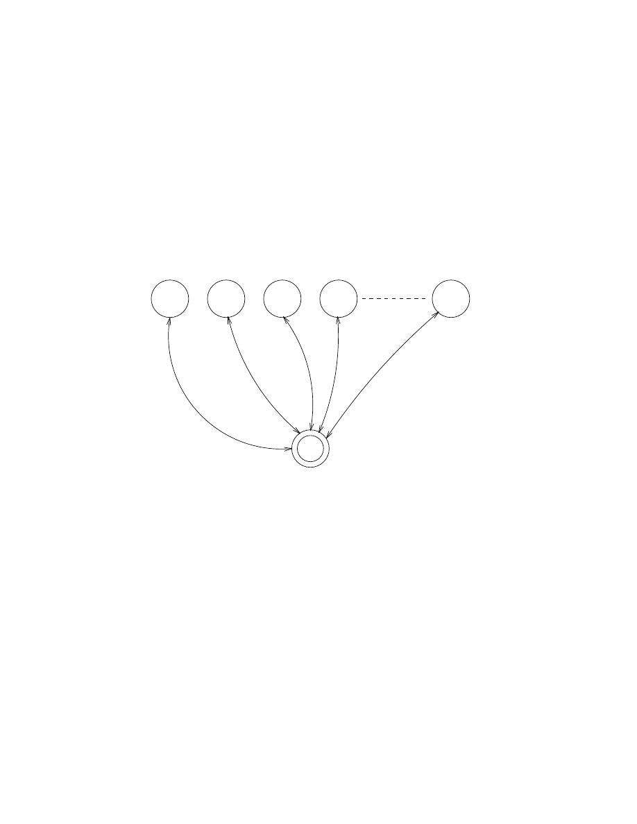
Robust Server Processes

111

8.2

Robust Server Processes

The design of a reliable server process is best described by way of an example.

Chapter ?? (Program ??.6) shows a resource allocator. In this allocator a

resource which has been allocated to a process will not be returned to the allocator
if the process making the allocation terminates (erroneously or normally) without
freeing the resource. This can be circumvented by:

• Setting the server to trap EXIT signals (process_flag(trap_exit, true)).

• Creating links between the allocator and processes which have allocated one

or more resources.

• Handling EXIT signals from such processes.

This is illustrated in Figure 8.1.

Process links

Allocator process

trapping EXIT signals

Client processes with allocated resources

Figure 8.1 Robust allocator process with clients

The access routines to the allocator are left unchanged. Starting the modified

allocator is done as follows:

start_server(Resources) ->

process_flag(trap_exit, true),
server(Resources, []).

The ‘server’ loop is modified to receive EXIT signals.

112

Programming Robust Applications

server(Free, Allocated) ->

receive

{From,alloc} ->

allocate(Free, Allocated, From);

{From,{free,R}} ->

free(Free, Allocated, From, R);

{’EXIT’, From, _ } ->

check(Free, Allocated, From)

end.

allocate/3 is modified so that we create a link to the process doing the alloca-

tion (if a resource is available).

allocate([R|Free], Allocated, From) ->

link(From),
From ! {resource_alloc,{yes,R}},
server(Free, [{R,From}|Allocated]);

allocate([], Allocated, From) ->

From ! {resource_alloc,no},
server([], Allocated).

free/4 becomes more complicated:

free(Free, Allocated, From, R) ->

case lists:member({R, From}, Allocated) of

true ->

From ! {resource_alloc, yes},
Allocated1 = lists:delete({R, From}, Allocated),
case lists:keysearch(From, 2, Allocated1) of

false ->

unlink(From);

_ ->

true

end,
server([R|Free], Allocated1);

false ->

From ! {resource_alloc, error},
server(Free, Allocated)

end.

First we check that the resource being freed really is allocated to the process

which is freeing it. lists:member({R,From}, Allocated) returns true if this is
the case. We create a new list of allocated resources as before. We cannot simply
unlink From, but must first check that From has not allocated other resources. If

Robust Server Processes

113

keysearch(From, 2, Allocated1)(see Appendix ??) returns false, From has
not allocated other resources and we can unlink From.

If a process to which we have created a link terminates, the server will receive

an EXIT signal and we call check(Free, Allocated, From).

check(Free, Allocated, From) ->

case lists:keysearch(From, 2, Allocated) of

false ->

server(Free, Allocated);

{value, {R, From}} ->

check([R|Free],

lists:delete({R, From}, Allocated), From)

end.

If lists:keysearch(From, 2, Allocated) returns false we have no resource

allocated to this process. If it returns {value, {R, From}} we see that resource
R has been allocated and we must add this to the list of free resources and delete
it from the list of allocated resources before continuing checking to see if any more
resources have been allocated by the process. Note that in this case we do not need
to unlink the process since it will already have been unlinked when it terminated.

Freeing an unallocated resource is probably a serious error. We could change

free/1 in Program ??.6 to kill the process doing the erroneous freeing:

free(Resource) ->

resource_alloc ! {self(),{free,Resource}},
receive

{resource_alloc, error} ->

exit(bad_allocation); % exit added here

{resource_alloc, Reply} ->

end.

A process which is killed in this way will, if it has allocated resources, be linked
to the server. The server will thus receive an EXIT signal which will be handled as
above and the allocated resources will be freed.

The above illustrates the following points:

• The interface to a server can be designed in such a way that clients use access

functions (in this case allocate/0 and free/1) and have no idea of what
goes on ‘behind the scenes’. The communication between clients and the
server process is hidden from the user. In particular, clients need not know
the process identity of the server and thus cannot interfere with its execution.

• A server which traps EXIT signals and creates links to its clients can monitor

clients and take appropriate actions if the clients die.

This is probably good programming practice since it will force programmers to correct such

errors.

114

Programming Robust Applications

8.3

Isolating Computations

In some applications we may wish to isolate a computation completely so that it
cannot influence other processes. The Erlang shell is such a case. The simple
shell in Chapter ?? is deficient. An expression evaluated in this shell can influence
the process performing the evaluation in a number of ways:

• It can send the identity of the process running the shell (self/0) to other

processes which can subsequently create links to this process or send it mes-
sages.

• It can register or unregister this process.

Program 8.1 is another way to write a shell:

-module(c_shell).
-export([start/0, eval/2]).

start() ->

process_flag(trap_exit, true),
go().

go() ->

eval(io:parse_exprs(’-> ’)),
go().

eval({form, Exprs}) ->

Id = spawn_link(c_shell, eval, [self(), Exprs]),
receive

{value, Res, _} ->

io:format("Result: ~w~n", [Res]),
receive

{’EXIT’, Id, _ } ->

true

end;

{’EXIT’, Id, Reason} ->

io:format("Error: ~w!~n", [Reason])

end;

eval(_) ->

io:format("Syntax Error!~n", []).

eval(Id, Exprs) ->

Id ! eval:exprs(Exprs, []).

Program 8.1

Keeping Processes Alive

115

The process running the shell traps EXIT signals. Commands are evaluated in

a separate process (spawn_link(c_shell, eval, [self(), Exprs])) which is
linked to the shell process. Despite the fact that we give c_shell:eval/2 the
process identity of the shell, this cannot be misused since it is not given as an
argument to the function doing the actual evaluation, eval:exprs/2.

8.4

Keeping Processes Alive

Some processes may be vital to the ‘well-being’ of a system. For example, in a
conventional time-sharing system, each terminal line is often served by a process
which is responsible for input and output to the terminal. If such a process dies the
terminal becomes unusable. Program 8.2 is a server which keeps processes alive by
re-creating any which terminate.

The server process which is registered as keep_alive maintains a list of tuples

{Id, Mod, Func, Args}, containing the process identity, the module, function
and arguments of the processes which it is keeping alive. It starts these processes
using the BIF spawn_link/3 so it is also linked to each such process. Since the
server traps EXITs, it receives an EXIT signal if any of the processes it is keeping
alive terminates. By searching the list of tuples it can re-create such a process.

Program 8.2, of course, needs improvement. As it stands it is impossible to

remove a process from the list of processes to keep alive. Also, if we try starting
a process for which the module:function/arity does not exist, the server will go
into an infinite loop. Creating a correct program without these deficiencies is left
as an exercise for the reader.

8.5

Discussion

The default action of a process which receives a signal in which the ‘reason’ is
not normal, is to terminate and propagate the signal to its links (see Section ??).
It is easy to create a layered operating system by using links and trapping EXIT
signals. Processes at the top layer of such a system (the application processes)
do not trap EXITs. Processes in the same transaction are linked to each other.
Lower layer processes (operating system processes) trap EXITs and have links to
application processes which they need to monitor (see Figure 8.2). Examples of this
type of operating system structure are the relations between the switch server and
telephony application processes in Chapter ?? and the file system in Chapter ??.

An application process which terminates abnormally causes EXIT signals to be

sent to all the processes in its transaction and thus kill the entire transaction. The
operating system processes which are linked to application processes in the failing
transaction also receive EXIT signals and can clean up undesired side-effects and
maybe restart the transaction.

116

Programming Robust Applications

-module(keep_alive).
-export([start/0, start1/0, new_process/3]).

start() ->

start1() ->

process_flag(trap_exit, true),
loop([]).

loop(Processes) ->

receive

{From, {new_proc, Mod, Func, Args}} ->

Id = spawn_link(Mod, Func, Args),
From ! {keep_alive, started},
loop([{Id, Mod, Func, Args}|Processes]);

{’EXIT’, Id, _} ->

case lists:keysearch(Id, 1, Processes) of

false ->

loop(Processes);

{value, {Id, Mod, Func, Args}} ->

P = lists:delete({Id,Mod,Func,Args},

Processes),

Id1 = spawn_link(Mod, Func, Args),
loop([{Id1, Mod, Func, Args} | P])

end

end.

new_process(Mod, Func, Args) ->

keep_alive ! {self(), {new_proc, Mod, Func, Args}},
receive

{keep_alive, started} ->

true

end.

Program 8.2

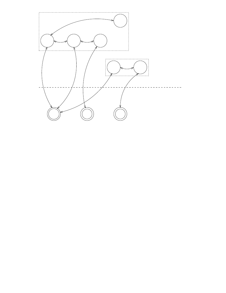
Discussion

117

Operating system

processes trapping EXIT

signals and linked

to application processes

Application processes

linked into transactions

Figure 8.2 Operating system and application processes

Chapter 9

Miscellaneous Items

This chapter deals with:

• Last call optimisation – This is an optimisation which allows tail recursive

programs to be evaluated in constant space.

• References – These provide names which are guaranteed to be unique on all

nodes.

• Code replacement – In an embedded real-time system code updates must be

made on the fly, that is, without stopping the system.

• Ports – These provide a mechanism for communicating with the external

world.

• Binaries – A built-in data type which can be used to store and manipulate

an area of untyped memory.

• Process dictionaries – These can be used in a process to store and retrieve

global data destructively.

• The net kernel – The net kernel is responsible for coordinating all network

operations in a distributed Erlang system.

• Hashing – This is a method of mapping a term onto a unique integer which

can be used to implement highly efficient table lookup methods.

• Efficiency – We discuss how to write efficient Erlang programs.

9.1

Last Call Optimisation

Erlang

provides last call optimisation, which allows functions to be evaluated in

constant space. The principal technique used to store persistent data is to store
it in structures which are manipulated in a server process (a typical example of
this was shown in Section ??). In order for such a technique to work correctly the
server must make use of the last call optimisation.

If this is not done then the server will eventually run out of space and the system

will not function correctly.

118

Last Call Optimisation

119

9.1.1

Tail recursion

We introduce the idea of tail recursion by showing how the same function can be
written in two different styles, one of which is tail recursive. Consider the function
length defined as follows:

length([_ | T]) ->

1 + length(T);

length([]) ->

Suppose we evaluate length([a, b, c]). The first clause defining length re-

duces the problem to evaluating 1 + length([b,c]). Unfortunately, the + op-
eration cannot be performed immediately but must be delayed until the value of
length([b, c]) is available. The system must remember that it has to perform
a + operation and at a later stage (when the value of length([b,c]) is known)
retrieve the fact that it has to do a + operation and then actually perform the
operation.

The pending operations are stored in a local data area. The size of this area

is at least K * N storage locations (where K is some constant representing the
overhead incurred in each new evaluation of length and N is the number of pending
operations).

We now write an equivalent function to compute the length of a list which makes

use of an accumulator (see Section ??) and which evaluates in constant space (we
call this length1 to avoid confusion):

length1(L) ->

length1(L, 0).

length1([_|T], N) ->

length1(T, 1 + N);

length1([], N) ->

To evaluate length1([a, b, c]) we first evaluate length1([a, b, c], 0).

This reduces to the evaluation of length1([b, c], 1 + 0). The + operation can
now be performed immediately (because both its arguments are known). Successive
function evaluations in the calculation of length1([a, b, c]) are thus:

length1([a, b, c])
length1([a, b, c], 0)
length1([b, c], 1 + 0)
length1([b, c], 1)
length1([c], 1 + 1)
length1([c], 2)

120

Miscellaneous Items

length1([], 1 + 2)
length1([], 3)
3

A tail recursive function is one which does not accumulate any pending opera-

tions before recursing. A clause is tail recursive if the last expression in the body of
the clause is a call to the function itself or a constant. A function is tail recursive
if all its clauses are tail recursive.

For example:

rev(X) -> rev(X, []).

rev([], X) -> X;
rev([H|T], X) -> rev(T, [H|X]).

is tail recursive, but:

append([], X) -> X;
append([H|T], X) -> [H | append(T, X)].

is not tail recursive since the last expression evaluated in the body of the second
clause (the | operation in [H|append(T,X)]) is neither a call to append nor a
constant.

9.1.2

Last call optimisation

Tail recursion is a special case of the more general last call optimisation (LCO).
The last call optimisation applies whenever the last expression occurring in the
body of a clause is a function evaluation.

For example:

g(X) ->

...
h(X).

h(X) ->

...
i(X).

i(X) ->

...
g(X).

defines a set of three mutually recursive functions. The LCO allows the evaluation
of g(X) to take place in constant space.

References

121

A careful examination of the server examples given in this book will reveal that

all are written so as to execute in constant

space.

9.2

References

References are unique objects. The BIF make_ref() returns a globally unique
object guaranteed to be different from every other object in the system and all
other (possibly) running Erlang nodes. The only thing that can be done with
references is to compare them for equality.

For example, we could use the following interface function in the client–server

model.

request(Server, Req) ->

Server ! {R = make_ref(), self(), Req},

receive

{Server, R, Reply} ->

end.

request(Server, Req) sends a request Req to the server with name Server; the
request contains a unique reference R. The reply from the server is checked to
ensure the presence of the unique reference R. This method of communication with
the server provides ‘end-to-end’ confirmation that the request has been processed.

9.3

Code Replacement

In an embedded real-time system we may wish to make code updates without
stopping the system. We may, for example, want to correct a software error in a
large telephone exchange without interrupting the service being offered.

Code replacement during operation is a common requirement in large ‘soft’ real-

time control systems which have a long operational life and a large volume of
software. It is not usually a requirement in dedicated ‘hard’ real-time software
which is often assigned to specific processors or burnt into ROM.

9.3.1

Example of code replacement

Consider Program 9.1.

We begin by compiling and loading the code for code_replace. Then we start

the program and send the messages hello, global and process to the process

Excepting, of course, for the space required for the local data structures of the server.

122

Miscellaneous Items

-module(code_replace).
-export([test/0, loop/1]).

test() ->

loop(N) ->

receive

X ->

io:format(’N = ~w Vsn A received ~w~n’,[N, X])

end,
code_replace:loop(N+1).

Program 9.1

which is created. Finally we edit the program, changing the version number from
A to B, recompile and load the program and send the process the message hello.

The following dialogue results:

%%% start by compiling and loading the code
%%%

(this is done by c:c)

c:c(code_replace).

...
> code_replace:test().
true
> global ! hello.
N = 0 Vsn A received hello
hello
> global ! global.
N = 1 Vsn A received global
global
> global ! process.
N = 2 Vsn A received process
%%% edit the file code_replace.erl
%%% recompile and load
> c:c(code_replace).
....
> global ! hello.
N = 3 Vsn B received hello

Here we see that the local variable N which is used as an argument to loop/1

is preserved despite the fact we have recompiled and loaded the code in loop/1
while it is being executed.

Observe that the server loop was written as follows:

Ports

123

-module(xyz).

loop(Arg1, ..., ArgN) ->

receive

...

end,
xyz:loop(NewArg1, ..., NewArgN).

This has a subtly different meaning from the code:

-module(xyz).

loop(Arg1, ..., ArgN) ->

receive

...

end,
loop(NewArg1, ..., NewArgN).

In the first case the call xyz:loop(...) means call the latest version of loop in
the module xyz. In the second case (without the explicit module name) it means
call the version of loop in the currently executing module.

Use of an explicitly qualified module name (module:func) causes module:func

to be dynamically linked into the run-time code. Every time a call is made using a
fully qualified module name the system will evaluate the function using the latest
available version of the code. Addresses of local functions within a module are
resolved at compile-time – they are static and cannot be changed at run-time.

In the example dialogue c:c(File) compiles and loads the code in File. This

is discussed in more detail in Section ??.

9.4

Ports

Ports provide the basic mechanism for communication with the external world.
Application programs written in Erlang may wish to interact with objects which
exist outside the Erlang system. When building complex systems it may be
desirable to interface Erlang programs to existing software packages, for exam-
ple windowing or database systems, or programs written in foreign languages, for
example, C or Modula2.

From the programmer’s point of view, it is desirable to view all activities occur-

ring outside Erlang as if they were programmed in Erlang. To create this
illusion we must arrange that objects outside Erlang behave as if they were
normal Erlang processes. To achieve this, an abstraction called a Port provides
a byte-oriented communication channel between Erlang and the external world.

Evaluating the expression open_port(PortName, PortSettings) creates a new

port which behaves in a similar manner to a process. The process which evaluates

124

Miscellaneous Items

open_port is called the connected process for the port. The purpose of the con-
nected process is to provide a destination for all incoming messages to the port.
An external object sends a message to Erlang by writing a sequence of bytes to
the port associated with that object. The port then sends a message containing
this sequence of bytes to the connected process.

Any process in the system can be linked to a port, and EXIT signals between

ports and Erlang processes behave exactly as if the port were an Erlang process.
Only three messages are understood by a port:

Port ! {PidC, {command, Data}}
Port ! {PidC, {connect, Pid1}}
Port ! {PidC, close}

PidC must be the Pid of the connected process. The meanings of these messages
are as follows:

{command, Data}

Send the bytes described by Data to the external object. Data is a possibly
non-flat

list whose individual elements are integers in the range 0.255 or a

single binary object. No reply.

Close the port. The port will reply by sending a {Port, closed} message
to the connected process.

{connect, Pid1}

Change the connected process of the port to Pid1. The port will reply by
sending a {Port, connected} message to the previously connected process.

In addition, the connected process can receive data messages with:

receive

{Port, {data, Data}} ->

... an external object has sent data to Erlang ...

...

end

In this section we will describe two programs which make use of a port: the first

is an Erlang process executing inside the Erlang workspace; the second is a C
program executing outside Erlang.

9.4.1

Opening ports

Ports can be opened with a number of different settings. To open a port the BIF
open_port(PortName, PortSettings) is used. PortName is one of:

A flat list is a list containing no sub-lists.

Ports

125

{spawn, Command}

Start an external program or start a driver with the name of Command if there
is one. Erlang drivers are described in Appendix E. Command is the name of
the external program which will be run. Command runs outside the Erlang
workspace if no driver with the name Command can be found.

Atom

Atom is assumed to be the name of an external resource. A transparent con-
nection between Erlang and the resource named by the atom is established.
The behaviour of connection depends upon the type of the resource. If Atom
represents a file then a single message is sent to the Erlang process con-
taining the entire contents of the file. Sending messages to the port causes
data to be written to the file.

{fd, In, Out}

Allow an Erlang process to access any currently opened file descriptors
used by Erlang. The file descriptor In can be used for standard input and
Out for standard output. Very few processes need to use this: only various
servers in the Erlang operating system (shell and user). Note this is very
UNIX-specific.

PortSettings is a list of settings for the port. Valid values are:

{packet, N}

Messages are preceded by their length, which is sent in N bytes with the most
significant byte first. Valid values for N are 1, 2 or 4.

stream

Output messages are sent without packet lengths – a private protocol must
be used between the Erlang process and the external object.

use_stdio

Only valid for {spawn, Command}. Make spawned (UNIX) process use stand-
ard input and output (i.e. file descriptors 0 and 1) for communicating with

Erlang

nouse_stdio

The opposite of above. Use file descriptors 3 and 4 for communicating with

Erlang

The port can be used for input only.

out

The port can be used for output only.

binary

The port is a binary port (described later).

eof

The port will not be closed on end of file and produce an ’EXIT’ signal,
rather it will remain open and send an {Port,eof} to the process that is
connected to the port, hence output can still be sent to the port.

126

Miscellaneous Items

The default is stream for all types of port and use_stdio for spawned ports.

9.4.2

The port as seen by an Erlang process

Program 9.2 defines a simple Erlang process which opens a port and sends it
a sequence of messages. The external object connected to the port processes and
replies to these messages. After a short delay the Erlang process closes the port.

-module(demo_server).
-export([start/0]).

start() ->

Port = open_port({spawn, demo_server}, [{packet, 2}]),
Port ! {self(), {command, [1,2,3,4,5]}},
Port ! {self(), {command, [10,1,2,3,4,5]}},
Port ! {self(), {command, "echo"}},
Port ! {self(), {command, "abc"}},
read_replies(Port).

read_replies(Port) ->

receive

{Port, Any} ->

io:format(’erlang received from port:~w~n’, [Any]),
read_replies(Port)

after 2000 ->

Port ! {self(), close},
receive

{Port, closed} ->

true

end

end.

Program 9.2

In Program 9.2 open_port(PortName, PortSettings) starts an external pro-

gram. demo_server is the name of the external program which will be run.

The expression Port ! {self(),

{command, [1,2,3,4,5]}} sends five bytes

(with values 1,2,3,4,5) to the external program.

To make things interesting the external program associated with the port in this

example has the following functionality:

• If the program is sent the string "echo" it sends the reply "ohce" to Erlang.

Ports

127

• If the server is sent a data block whose first byte is 10 it replies with a block

where all the elements in the block except the first have been doubled.

• Otherwise the data is ignored.

Running the program we obtain the following:

> demo_server:start().
erlang received from port:{data,[10,2,4,6,8,10]}
erlang received from port:{data,[111,104,99,101]}
true

9.4.3

The port as seen by an external process

The external program which executes outside the Erlang system (as started by
open_port({spawn, demo_server}, [{packet,2}])) can be written in any pro-
gramming language supported by the host operating system. Our examples assume
that we are running on a UNIX system and that the external program is a UNIX
process which is programmed in C.

The C program which communicates with the Erlang process shown in Sec-

tion ?? is given in Program 9.3. This should be compiled and made into an
executable file called demo_server.

/* demo_server.c */
#include <stdio.h>
#include <string.h>

/* Message data are all unsigned bytes */
typedef unsigned char byte;

main(argc, argv)
int argc;
char **argv;
{

int len;
int i;
char *progname;
byte buf[1000];

progname = argv[0];

/* Save start name of program */

fprintf(stderr, "demo_server in C Starting \n");

128

Miscellaneous Items

while ((len = read_cmd(buf)) > 0){

if(strncmp(buf, "echo", 4) == 0)

write_cmd("ohce", 4);

else if(buf[0] == 10){

for(i=1; i < len ; i++)

buf[i] = 2 * buf[i];

write_cmd(buf, len);

}

/* Read the 2 length bytes (MSB first), then the data. */
read_cmd(buf)
byte *buf;
{

int len;

if (read_exact(buf, 2) != 2)

return(-1);

len = (buf[0] << 8) | buf[1];
return read_exact(buf, len);

}

/* Pack the 2

bytes length (MSB first) and send it */

write_cmd(buf, len)
byte *buf;
int len;
{

byte str[2];

put_int16(len, str);
if (write_exact(str, 2) != 2)

return(-1);

return write_exact(buf, len);

}

[read|write]_exact are used since they may return

BEFORE all bytes have been transmitted

read_exact(buf, len)
byte *buf;
int

len;

{

int i, got = 0;

Ports

129

do {

if ((i = read(0, buf+got, len-got)) <= 0)

return (i);

got += i;

} while (got < len);
return (len);

}

write_exact(buf, len)
byte *buf;
int

len;

{

int i, wrote = 0;

do {

if ((i = write(1, buf+wrote, len-wrote)) <= 0)

return (i);

wrote += i;

} while (wrote < len);
return (len);

}

put_int16(i, s)
byte *s;
{

*s = (i >> 8) & 0xff;
s[1] = i & 0xff;

}

Program 9.3

Program 9.3 reads the byte sequence which was sent to the Erlang port

with the expression len = read_cmd(buf) and sends data back to Erlang with
write_cmd(buf, len).

File descriptor 0 is used to read data from Erlang and file descriptor 1 is used

to write data to Erlang. The C routines do the following:

read_cmd(buf)

Reads a single command from Erlang.

write_cmd(buf, len)

Writes a buffer of length len to Erlang.

read_exact(buf, len)

Reads exactly len bytes.

130

Miscellaneous Items

write_exact(buf, len)

Writes len bytes.

put_int16(i, s)

Packs a 16-bit integer into two bytes.

The routines read_cmd and write_cmd assumes that the protocol between the

external server and Erlang consists of a two-byte header, giving the length of
the data packet to be exchanged, followed by the data itself. This is illustrated in
Figure 9.1.

Erlang

[0,5,1,2,3,4,5]

Port ! {command, [1,2,3,4,5]}

len = read(0, buf, 2)

len = (buf[0]<<8)|buf[1];

read(0, buf, len);

Figure 9.1 Communication with a port

This particular protocol (two-byte header plus data) was used since the port was

opened by evaluating:

open_port({spawn, demo_server}, [{packet, 2}])

9.5

Binaries

A binary is a data type which is used to store an area of untyped memory. A port
is a binary port if the atom binary appears in the Settings list, given as the
last argument to open_port/2. All messages which come from a binary port are
binaries.

To illustrate the difference between a binary and normal port assume that we

wish to send the string "hello" from an external process to the Erlang system
and that the ‘two-byte header plus data’ convention is used. The external program
outputs the following byte sequence:

0 5 104 101 108 108 111

If the Erlang process which is connected to the port is a normal port, then

the message {Port, {data, [104,101,108,108,111]}} will be sent to the pro-
cess.

If the port had been a binary port then the message would have been

{Port, {data, Bin}}, where Bin is a binary data object of size 5, storing the
bytes of the message. Note that in both cases there is no change to the external
process which sends data to the port.

The advantage of having the port sending binary data objects instead of lists is

that if the lists are long, it is considerably faster to build and send a binary data
object than a list.

The following BIFs are used to manipulate binaries:

Binaries

131

term_to_binary(T)

Converts the term T to a binary. The resulting binary data object is a
representation of the term in the external term format.

binary_to_term(Bin)

Is the inverse of term_to_binary/1.

binary_to_list(Bin)

Converts the binary Bin to a list of integers.

binary_to_list(Bin, Start, Stop)

Converts a portion of the binary Bin into a list of characters, starting at
position Start, and stopping at position Stop. The first position of the
binary has position 1.

list_to_binary(Charlist)

Converts Charlist into a binary data object.

This is not the same as

term_to_binary(Charlist). This BIF builds a binary object containing the
bytes in Charlist as opposed to term_to_binary(Charlist) which builds
a binary object containing the bytes of the external term format of the term
Charlist.

split_binary(Bin, Pos)

Builds two new binaries, as if Bin had been split at Pos. Returns a tuple
consisting of the two new binaries. For example:

1> B = list_to_binary("0123456789").
#Bin
2> size(B).
10
3> {B1,B2} = split_binary(B,3).
{#Bin,#Bin}
4> size(B1).
3
5> size(B2).
7

concat_binary(ListOfBinaries)

Returns a new binary which is formed by the concatenation of the binaries
in ListOfBinaries.

In addition the guard test binary(X) succeeds if X is a binary data object.

Binaries are primarily used for code loading in a network, but can also be used by
applications that shuffle large amounts of raw data such as audio or video data. It
is possible to efficiently input very large amounts of binary data through a port,
work with the data , and then at a later stage, output it to another or the same
port.

132

Miscellaneous Items

9.6

Process Dictionary

Each process has an associated dictionary. This dictionary can be manipulated
with the following BIFs:

put(Key, Value).

Erlang

terms.

get(Key).

Returns the value associated with Key in the process dictionary. Returns
undefined if no value is associated with Key.

get().

Returns the entire process dictionary as a list of {Key, Value} tuples.

get_keys(Value).

Returns a list of keys which correspond to Value in the process dictionary.

erase(Key).

Returns the value associated with Key and deletes it from the process diction-
ary. Returns undefined if no value is associated with Key.

erase().

Returns the entire process dictionary and deletes it.

The process dictionary is local to each process. When a process is spawned the

dictionary is empty. Any function can add a {Key, Value} association to the
dictionary by evaluating put(Key, Value), the value can be retrieved later by
evaluating get(Key). Values stored when put is evaluated within the scope of a
catch will not be ‘retracted’ if a throw is evaluated or an error occurs.

The entire dictionary can be retrieved with get() or erased with erase(). In-

dividual items can be erased with erase(Key).

We sometimes wish to access the same global data in many different functions

and it can be somewhat inconvenient to pass this data as arguments to all functions
in a process. This can be avoided by careful use of put and get.

The use of get and put introduces destructive operations into the language and

allows the programmer to write functions with side-effects. The result of eval-
uating such functions may depend upon the order in which they are evaluated.
The process dictionary should be used with extreme care. get and put are anal-
ogous to gotos in conventional imperative languages; they are useful in certain
restricted circumstances but their use leads to unclear programs and should be
avoided wherever possible. None of the programs in this book makes use of the
process dictionary since we do not wish to encourage its use – it is included here
and in the appendices for completeness.

The Net Kernel

133

9.7

The Net Kernel

The net_kernel is a process which is used used to coordinate operations in a
distributed Erlang system. The run-time system automatically sends certain
messages to the net_kernel. The code executing in this process decides which
action to take when different system messages arrive.

An Erlang system can be run in one of two modes. It can either run as a closed

system which cannot communicate with other Erlang systems, or it can run as
a system which can communicate with other systems, in which case it is said to
be alive. A system is made alive by evaluating the BIF alive/2. This is normally
done by the Erlang operating system and not by the user directly. The call:

erlang:alive(Name, Port)

informs a network name server that an Erlang system has been started and is
available to cooperate in distributed computations.

Name is a atom containing the local name by which the Erlang system will

be known. The external name of this Erlang system will be Name@MachineName
where MachineName is the name of the machine where the node resides and the char-
acter ’@’ is used to separate the local name and the machine name. For example,
evaluating erlang:alive(foo,Port) on a host called super.eua.ericsson.se
will start an Erlang system with the name foo@super.eua.ericsson.se which
is globally unique. Several different Erlang systems can run on the same machine
provided they all have different local names.

Port is an Erlang port. The external port program must comply with the

internal Erlang distribution protocol. This program is responsible for all net-
working operations, such as establishing communication channels to remote nodes
and reading or writing buffers of bytes to these nodes. Different versions of the
port program allows Erlang nodes to communicate using different networking
technologies.

Evaluating alive/2 causes the node evaluating the expression to be added to a

pool of Erlang nodes which can engage in distributed computations. The process
evaluating alive/2 must be registered with the name net_kernel. If this is not
the case, the BIF will fail. To disconnect a node from the network, the distribution
port can be closed.

To check whether an Erlang system is alive or not, the BIF is_alive() can

be used. This BIF returns either true or false.

Whenever a new node becomes known a {nodeup, Node} message is sent to the

net_kernel, and whenever a node fails a {nodedown, Node} message is sent to the
net_kernel. All requests to create new processes with spawn/4 or spawn_link/4,
as well as all requests to send a message to a remotely registered process with the
construction {Name, Node} ! Message, go through the net_kernel process. This
enables user defined net_kernel code for different purposes. For example, the BIF
spawn/4 is implemented in Erlang itself. The client code to create a process at
a remote node is:

134

Miscellaneous Items

spawn(N,M,F,A) when N /= node() ->

monitor_node(N, true),
{net_kernel, N} ! {self(), spawn, M, F, A, group_leader()},
receive

{nodedown, N} ->

R = spawn(erlang, crasher, [N,M,F,A,noconnection]);

{spawn_reply, Pid} ->

R = Pid

end,
monitor_node(N, false),
R;

spawn(N,M,F,A) ->

spawn(M,F,A).

crasher(Node,Mod,Fun,Args,Reason) ->

exit(Reason).

This code will result in a message to the net_kernel at the remote node. The

remote net_kernel is responsible for creating a new process, and replying to the
client with the Pid of the new process.

9.7.1

Authentication

The Erlang system has built-in support for authentication which uses the idea
of ‘magic cookies’. A magic cookie is a secret atom assigned to each node. When
started, each node is automatically assigned a random cookie. In order for node
N1 to communicate with node N2, it must know which magic cookie N2 has. How
N1 finds out what N2’s cookie is, is not discussed here. For N1 to communicate
with N2 it must evaluate erlang:set_cookie(N2, N2Cookie) where N2Cookie is
the value of N2’s cookie. In addition, for N1 to be able to receive a response from
N2, N2 must evaluate erlang:set_cookie(N1, N1Cookie) where N1Cookie is the
value of N1’s cookie.

The Erlang run-time system will insert the cookie in all messages it sends to all

remote nodes. If a message arrives at a node with the wrong cookie, the run-time
system will transform that message into a message of the form:

{From,badcookie,To,Message}

Where To is the Pid or the registered name of the intended recepient of the message
and From is the Pid of the sender. All unauthorised attempts either to send a
message or to spawn a process will be transformed into badcookie messages and
sent to the net_kernel. The net_kernel can choose to do whatever it likes with
these badcookie messages.

Two BIFs are used to manipulate cookies:

The Net Kernel

135

erlang:get_cookie()

Returns our own magic cookie.

erlang:set_cookie(Node,Cookie)

Sets the magic cookie of Node to be Cookie. This can be used once the
cookie of Node has been obtained. It will cause all messages to Node to
contain Cookie. If Cookie really is the magic cookie of Node the messages
will go directly to the recipient at Node. If it is the wrong cookie, the message
will be transformed into a badcookie message at the receiving end, and then
sent to the net_kernel there.

By default all nodes assume that the atom nocookie is the cookie of all other

nodes, thus initially all remote messages will contain the cookie nocookie.

If the value of Node in the call erlang:set_cookie(Node, Cookie) is the name

of the local node then the magic cookie of the local node is set to Cookie, in
addition, all other nodes having cookies with the value nocookie have their cookie
changed to Cookie. If all nodes start by evaluating:

erlang:set_cookie(node(), SecretCookie),

then they will all automatically be authenticated to cooperate with each other.
How the application obtains the SecretCookie is a local issue. The secret cookie
could be stored in a read-by-user, or read-by-group only file.

In a UNIX environment the default behaviour when starting a node is to read a

file in the user’s HOME directory called .erlang.cookie. A check is done to ensure
that the file is properly protected, and erlang:set_cookie(node(), Cookie) is
then evaluated, where Cookie is the contents of the cookie file as an atom. Hence
the same user will be able to communicate safely with all other Erlang nodes
which are running with the same user id (assuming that the nodes reside on the
same file system). If the nodes reside on different file systems, the user must only
ensure that the cookie file on all involved file systems are identical.

9.7.2

The net kernel messages

The following is a list of the messages which can be sent to the net_kernel:

• {From,registered_send,To,Mess} A request to send the message Mess to

the registered process To.

• {From,spawn,M,F,A,Gleader} A request to create a new process. Gleader

is the group leader of the requesting process.

• {From,spawn_link,M,F,A,Gleader} A request to create a new process and

set up a link to the new process.

• {nodeup,Node} Whenever the system gets connected to a new node, this

message is sent to the net_kernel. This can either be the result of a remote
node contacting us, or that a process running at this node tried (successfully)
to do a remote operation for the first time.

136

Miscellaneous Items

• {nodedown,Node} Whenever an existing node fails or a local attempt to

contact a remote node fails, this message is sent to the net_kernel.

• {From,badcookie,To,Mess} Whenever a non-authenticated attempt to com-

municate with this node is done, a message indicating the nature of the at-
tempt is sent to the net_kernel. For example, an attempt to create a new
process from an un-authenticated node, will result in a

{From,badcookie, net_kernel, {From,spawn,M,F,A,Gleader}}

message being sent to the net_kernel.

Since the net_kernel runs as a user-defined process, it is possible to modify it

to employ different user-defined authentication schemas. For example, if we want
to have a node that disallows all remote interactions except messages sent to a
special safe process called safe, we merely have to let our net_kernel ignore all
attempts to create new processes and all attempts to send a message to any other
process but the one called safe.

9.8

Hashing

Erlang

has a BIF which produces an integer hash value from an arbitrary term:

hash(Term, MaxInt)

Returns an integer in the range 1..MaxInt.

We can use the hash BIF to write a highly efficient dictionary lookup program.

The interface to this program is almost identical to the binary tree implementation
of a dictionary given in Section ??

-module(tupleStore).
-export([new/0,new/1,lookup/2,add/3,delete/2]).

new() ->

new(256).

new(NoOfBuckets) ->

make_tuple(NoOfBuckets, []).

lookup(Key, Tuple) ->

lookup_in_list(Key, element(hash(Key, size(Tuple)), Tuple)).

add(Key, Value, Tuple) ->

Index = hash(Key, size(Tuple)),
Old

= element(Index, Tuple),

New

= replace(Key, Value, Old, []),

setelement(Index, Tuple, New).

Hashing

137

delete(Key, Tuple) ->

Index = hash(Key, size(Tuple)),
Old

= element(Index, Tuple),

New

= delete(Key, Old, []),

setelement(Index, Tuple, New).

make_tuple(Length, Default) ->

make_tuple(Length, Default, []).

make_tuple(0, _, Acc) ->

list_to_tuple(Acc);

make_tuple(N, Default, Acc) ->

make_tuple(N-1, Default, [Default|Acc]).

delete(Key, [{Key,_}|T], Acc) ->

lists:append(T, Acc);

delete(Key, [H|T], Acc) ->

delete(Key, T, [H|Acc]);

delete(Key, [], Acc) ->

Acc.

replace(Key, Value, [], Acc) ->

[{Key,Value}|Acc];

replace(Key, Value, [{Key,_}|T], Acc) ->

[{Key,Value}|lists:append(T, Acc)];

replace(Key, Value, [H|T], Acc) ->

replace(Key, Value, T, [H|Acc]).

lookup_in_list(Key, []) ->

undefined;

lookup_in_list(Key, [{Key, Value}|_]) ->

{value, Value};

lookup_in_list(Key, [_|T]) ->

lookup_in_list(Key, T).

Program 9.4

The only difference between this and Program ??.4 is in the function new/1,

where we need to supply the size of the hash table.

Program ??.4 is a simple implementation of a conventional hash lookup program.

The hash table, T, is represented as a fixed size tuple. To lookup the value of the
term Key a hash index, I, is computed in the range 1..size(T). element(I, T)
contains a list of all {Key, Value} pairs which hash to the same index. This list
is searched for the desired {Key, Value} pair.

138

Miscellaneous Items

To insert in the hash table Key is hashed to an integer index I, and a new

{Key, Value} pair is inserted into the list found in element(I, T) of the hash
table. Any old association with Key is lost.

The module tupleStore provides a highly efficient dictionary. For efficient ac-

cess the size of the hash table should be larger than the number of elements to
be inserted in the table.

While lookup in such a structure is highly efficient,

insertion is less so.

This is because in most implementations of Erlang the

setelement(Index, Val, T) BIF creates an entirely new copy of the tuple T
each time it is called.

9.9

Efficiency

The topic of efficiency comes last in our discussion of miscellaneous items. This
is not because we consider the topic unimportant but because we believe that
premature concern for efficiency often leads to poor program design. The primary
concern must always be one of correctness, and to this aim we encourage the
development of small and beautiful algorithms which are ‘obviously’ correct.

As an example we show how an inefficient program can be turned into an efficient

program.

As an exercise we start with a file of tuples with information about employees

at a fictitious company, the file has entries such as:

{202191,’Micky’,’Finn’,’MNO’,’OM’,2431}.
{102347,’Harvey’,’Wallbanger’,’HAR’,’GHE’,2420}.
... 2860 lines omitted ...
{165435,’John’,’Doe’,’NKO’,’GYI’, 2564}.
{457634,’John’, ’Bull’,’HMR’,’KIO’, 5436}.

We want to write a program which inputs this data, builds each item into a

dictionary accesses each item once, and writes the data back to a file. We want to
run this program on a routine basis so we should make it as efficient as possible.

We will treat the input/output and access parts of the problem separately.

9.9.1

File access

The simplest approach we could use to input the file of tuples described above
would be to use file:consult(File) to read the file (see Appendix C) – this
takes rather a long time since each line has to be read and then parsed. A better
approach is to change the format of the input file from a text to a binary file. This
can be done as with the following function:

Efficiency

139

reformat(FileOfTerms, BinaryFile) ->

{ok, Terms} = file:consult(FileOfTerms),
file:write_file(BinaryFile, term_to_binary(Terms)).

To read the binary file and recover the original data we evaluate:

read_terms(BinaryFile) ->

{ok, Binary} = file:read(BinaryFile),
binary_to_term(Binary).

Reading a binary file and converting the result to a term is a lot faster than

reading and parsing a list of terms, as can be seen from the following table:

Text Size

Binary Size

file:consult

read terms

Ratio of

bytes

times

128041

118123

42733

783

54.6

4541

4190

1433

89.6

For a 4.5 Kbyte file reading was 90 times faster and for a 128 Kbyte file 55 times

faster; note also that the resulting binary file is somewhat smaller than the text
file.

9.9.2

Dictionary access

We used three different methods to build and update a dictionary of employees.
These methods were:

lists

All employees records are kept in a list. Initial insertion is done by adding
to the head of the list and updating by a linear scan through the list.

avl

The AVL tree insertion algorithms of Section ??.

hash

The hashing algorithm of Program ??.4.

To see the effect of these different methods we did a single insertion and single

lookup of each tuple in our employee data, this yielded the following timings:

#entries

AVL

list

hash

insert

lookup

insert

lookup

insert

lookup

5.32

0.00

0.64

1.32

0.00

1.32

0.32

0.00

1.00

0.32

0.00

100

2.00

0.50

0.00

1.50

0.33

0.16

200

9.91

0.50

0.00

3.00

2.08

0.17

400

28.29

0.46

0.04

5.96

4.25

0.09

800

301.38

0.54

0.02

11.98

1.77

0.15

1600

1060.44

0.61

0.02

24.20

4.05

0.14

140

Miscellaneous Items

In the above table the units are milliseconds per insertion or milliseconds per
lookup. We see that for tables of size greater that 800 hash lookup is always the
fastest lookup method.

From the above we can see that a program which used binary file input together

with a hash algorithm for lookup would be approximately six thousand times faster
than a program using file:consult togther with a simple list lookup method. As
with conventional imperative languages, the most important factor determining
program efficiency is good algorithm design.

Part II

Applications

Bibliography

[1] Adelson-Velskii, G.M. and Landis E.M., “An algorithm for the organisation of information”,

Doklady Akademia Nauk SSSR, 146 , (1962), 263–266; English translation in Soviet Math,
3, 1259–63.

[2] Ahlberg, I., Bauner, J-O. and Danne, A., “Prototyping cordless using declarative program-

ming”, International Switching Symposium, October 25–30, 1992, Yokohama.

[3] Armstrong, J. L., Virding, S. R. and Williams, M. C., “Use of Prolog for developing a new

programming language”, The Practical Application of Prolog, 1–3 April 1992, Institute of
Electrical Engineers, London.

[4] Agha, Gul A., Actors: A Model of Concurrent Computation in Distributed Systems, MIT

Press, 1986.

[5] Bal, H. Programming Distributed Systems, Prentice Hall 1990.

[6] Birell ,A D, Nelsson, B. J. “Implementing remote procedure calls” ACM Trans. Comp. Syst.,

2, (1) 1984.

[7] Bernstein, P., Hadzilacos ,V., Goodman, N. Concurrency Control and Recovery in Database

Systems, Addison-Wesley 1987

[8] Booch, G., Object–oriented Design with Applications, Benjamin-Cummings Publishing

Company, 1991.

[9] Bratko, I., Prolog Programming for Artificial Intelligence, Addison-Wesley, 1986, pp. 241–

245.

[10] Case, Jeffrey D., Feodor, Mark S., Shoffstall, Martin L. and Davin, James R., “A Simple

Network Management Protocol”, Request For Comment 1098, April 1989.

[11] CCITT Specification and Description Language (SDL), Recommendation X.100, Geneva,

Switzerland.

[12] CCITT Specification of Abstract Syntax Notation One (ASN.1), Recommendation X.208,

Geneva, Switzerland.

[13] CCITT Specification of Basic Encoding Rules (BER for Abstract Syntax One (ASN.1),

Recommendation X.209, Geneva, Switzerland.

[14] Gray, Jim and Reuter, Andreas Transaction Processing Concepts and Techniques, Morgan

Kaufmann Publishers, 1993.

143

144

Bibliography

[15] Clocksin, W. F. and Mellish, C. S., Programming in Prolog, Springer-Verlag, 1981.

[16] Coed, P. and Yourdon, E., Object-oriented Analysis, Yourdon Press, 1991.

[17] Coed, P. and Yourdon, E., Object-oriented Design, Yourdon Press, 1991.

[18] Eriksson, D., Persson, M. and ¨

Odling, K., “A switching software architecture prototype using

a real-time declarative language”, International Switching Symposium, October 25–30, 1992,
Yokohama.

[19] Jacobson, I., Christerson, M., Jonsson, P. and ¨

Overgaard, G., Object-oriented Software

Engineering, Addison-Wesley, 1992.

[20] Lamport, L., “Time, clocks and the ordering of events in a distributed system” Comm.

ACM , 21(7), July, 1978.

[21] Liskov, B. “Linguistic support for efficient asynchronous calls in distributed systems”. Pro-

ceedings of the SIGPLAN, 1988.

[22] Foster, I. and Taylor, S., STRAND: New Concepts in Parallel Processing, Prentice Hall,

1989.

[23] “SunOs 4.0 reference manual V. 10” 1987 Sun Microsystems, Inc.

[24] Open Systems Interconnection: Basic reference model. International Oganization for Stan-

dardization and Electrotechnical Committee, 1984.

[25] Sollins, K. R., “The TFTP Protocol (Revision 2)”, Request For Comment 783, June 1981.

[26] Stroustrup, B., The C++ Programming Language, 2nd edition, Addison-Wesley, 1991.

[27] Ullman, J. D., Principles of Database and Knowledgebase Systems, Computer Science Press,

1988.

[28] Wikstr¨

om, ˚

A., Functional Programming Using Standard ML, Prentice Hall, 1987.

[29] Wirth, N., Algorithms + Data Structures = Programs, Prentice Hall, 1976, pp. 215–226.

[30] Kunz, T. “The influence of different workload descriptions on a heuristic load balancing

scheme”. IEEE Trans. Software Eng., 17, (7), July, 1991 pp. 725-730.

Appendix A

ERLANG Reference Grammar

The Erlang reference grammar which follows is an adaptation of an LALR(1)
grammar for Erlang.

This grammar differs from a strict LALR(1) grammar in the treatment of the

production for the non-terminal “match expr”. In this case the expression to the
left-hand side of the “=” symbol could be a pattern or an expression – the ambiguity
is resolved in the semantic phase of the Erlang compiler.

Type

Precedence Operator

Nonassoc

’catch’.

Right

200

’=’.

Right

200

’ !’.

Left

300

add op.

Left

400

mult op.

Nonassoc

500

prefix op.

Line Non-terminal

Productions

add op

:= ”+”
| ”-”

| ”bor”

| ”bxor”

| ”bsl”

| ”bsr”

comp op

:= ”==”
| ”/=”

| ”=<”

| ”<”

| ”>=”

| ”>”

| ”=:=”

145

146

ERLANG Reference Grammar

| ”=/=”

mult op

:= ”*”
| ”/”

| ”div”

| ”rem”

| ”band”

prefix op

:= ”+”
| ”-”

| ”bnot”

basic type

:= ”atom”
| ”number”

| ”string”

| ”var”

| ”true”

pattern

:= basic type
| pattern list

| pattern tuple

pattern list

:= ”[” ”]”
| ”[” pattern pattern tail ”]”

pattern tail

:= ”

|” pattern

| ”,” pattern pattern tail

pattern tuple

:= ”

{” ”}”

| ”{” patterns ”}”

patterns

:= pattern
| pattern ”,” patterns

expr

:= basic type
| list

| tuple

| function call

| expr add op expr

| expr mult op expr

| prefix op expr

| ”(” expr ”)”

| ”begin” exprs ”end”

| ”catch” expr

| case expr

| if expr

| receive expr

| match expr

| send expr

list

:= ”[” ”]”
| ”[” expr expr tail ”]”

ERLANG Reference Grammar

147

expr tail

:= ”

|” expr

| ”,” expr expr tail

tuple

:= ”

{” ”}”

| ”{” exprs ”}”

function call

:= ”atom” ”(” parameter list ”)”
| ”atom” ”:” ”atom” ”(” parameter list ”)”

parameter list

:= exprs
|

case expr

:= ”case” expr ”of” cr clauses ”end”

cr clause

:= pattern clause guard clause body

cr clauses

:= cr clause
| cr clause ”;” cr clauses

if expr

:= ”if” if clauses ”end”

if clause

:= guard clause body

if clauses

:= if clause
| if clause ”;” if clauses

receive expr

:= ”receive” ”after” expr clause body ”end”
| ”receive” cr clauses ”end”

| ”receive” cr clauses ”after” expr clause body ”end”

match expr

:= expr ”=” expr

send expr

:= expr ”!” expr

exprs

:= expr
| expr ”,” exprs

guard expr

:= basic type
| guard expr list

| guard expr tuple

| guard call

| ”(” guard expr ”)”

| guard expr add op guard expr

| guard expr mult op guard expr

| prefix op guard expr

guard expr list

:= ”[” ”]”
| ”[” guard expr guard expr tail ”]”

guard expr tail

:= ”

|” guard expr

| ”,” guard expr guard expr tail

guard expr tuple

:= ”

{” ”}”

| ”{” guard exprs ”}”

guard exprs

:= guard expr
| guard expr ”,” guard exprs

guard call

:= ”atom” ”(” guard parameter list ”)”

guard parameter list

:= guard exprs

148

ERLANG Reference Grammar

bif test

:= ”atom” ”(” guard parameter list ”)”

guard test

:= bif test
| guard expr comp op guard expr

guard tests

:= guard test
| guard test ”,” guard tests

guard

:= ”true”
| guard tests

function clause

:= clause head clause guard clause body

clause head

:= ”atom” ”(” formal parameter list ”)”

formal parameter list := patterns

clause guard

:= ”when” guard
|

clause body

:= ”->” exprs

function

:= function clause
| function clause ”;” function

attribute

:= pattern
| ”[” farity list ”]”

| ”atom” ”,” ”[” farity list ”]”

farity list

:= farity
| farity ”,” farity list

farity

:= ”atom” ”/” ”number”

form

:= ”-” ”atom” ”(” attribute ”)”
| function

Non-terminal

Line Numbers

add op

*1 11 27

attribute

*44 47

basic type

*5 6 11 27

bif test

*34 35

case expr

11 *17

clause body

18 21 23 38 *42

clause guard

18 38 *41

clause head

38 *39

comp op

*2 35

cr clause

*18 19

cr clauses

17 *19 19 23

expr

*11 11 12 13 17 23 24 25 26

expr tail

12 *13 13

exprs

11 14 16 *26 26 42

farity

45 *46

farity list

44 *45 45

ERLANG Reference Grammar

149

form

*47

formal parameter list 39 *40
function

*43 43 47

function call

11 *15

function clause

*38 43

guard

21 *37 41

guard call

27 *32

guard expr

*27 27 28 29 31 35

guard expr list

27 *28

guard expr tail

28 *29 29

guard expr tuple

27 *30

guard exprs

30 *31 31 33

guard parameter list

32 *33 34

guard test

*35 36

guard tests

*36 36 37

if clause

*21 22

if clauses

20 *22 22

if expr

11 *20

list

11 *12

match expr

11 *24

mult op

*3 11 27

parameter list

15 *16

pattern

*6 7 8 10 18 44

pattern list

6 *7

pattern tail

7 *8 8

pattern tuple

6 *9

patterns

9 *10 10 40

prefix op

*4 11 27

receive expr

11 *23

send expr

11 *25

tuple

11 *14

Appendix B

Built-in Functions

Appendix B contains descriptions of Erlang’s built-in functions. BIFs are, by
convention, regarded as being in the module erlang.

Thus both of the calls

atom_to_list(’Erlang’) and erlang:atom_to_list(’Erlang’) are considered
identical.

BIFs may fail for a variety of reasons. All BIFs fail if they are called with

arguments of incorrect type. For example, atom_to_list/1 will fail if it is called
with an argument which is not an atom. If this type of failure is not caught (or
the BIF is not called within a guard – see below), it will cause the process making
the call to exit and an EXIT signal with reason badarg will be sent to all processes
which are linked. The other reasons why BIFs may fail are given together with the
description of each BIF.

A few BIFs may be used in guard tests (a complete list is given in the table in

Section ??). For example:

tuple_5(Something) when size(Something) == 5 ->

is_tuple_size_5;

tuple_5(_) ->

is_something_else.

Here the BIF size/1 is used in a guard. If size/1 is called with a tuple it will
return the size of the tuple (i.e. how many elements there are in the tuple). In the
example above size/1 is used in a guard which tests if its argument Something
is a tuple and , if it is a tuple, whether it is of size 5. In this case calling size with
an argument other than a tuple will cause the guard to fail and execution will
continue with the next guard. Suppose tuple_5/1 is written as follows:

tuple_5(Something) ->

case size(Something) of

5 -> is_tuple_size_5;

_ -> is_something_else

end.

150

The BIFs

151

In this case size/1 is not in a guard. If Something is not a tuple size/1 will fail
and cause the process to fail , with reason badarg (see above).

Some of the BIFs in this chapter are optional to Erlang implementations, i.e.

not all implementations will contain these BIFs. These BIFs cannot be called
by their names alone, but must be called using the module name erlang. For
example, erlang:load_module(xyz).

The descriptions which follow indicate which BIFs can be used in guards and

which BIFs are optional.

B.1

The BIFs

abs(Number)

Returns an integer or float which is the arithmetic absolute value of the argument
Number (integer or float).

> abs(-3.33).
3.3300000000000000e+00
> abs(-3).
3

This BIF is allowed in guard tests.

Failure: badarg if the argument is not an integer or a float.

alive(Name,Port)

The alive/2 BIF publishes the name Name as a symbolic name of our node. This
must be done if we want to communicate with other nodes, or want other nodes
to be able to communicate with us. Once this BIF returns the system is a node.
The argument Port must be a port (a driver or an external port program) that
can understand the internal Erlang distribution protocol.

This BIF designates the given port as a special ‘distribution’ port.
Optional BIF.

Failure: badarg If the net_kernel is not running or if the parameters Port and
Name ar not a port and an atom, respectively.

apply(Module, Function, ArgumentList)

Returns the result of applying Function in Module to ArgumentList. The applied
function must have been exported from the Module. The arity of the function is
the length of the ArgumentList.

152

Built-in Functions

> apply(lists, reverse, [[a, b, c]]).
[c, b, a]

BIFs themselves can be applied by assuming they are exported from the module

erlang.

> apply(erlang, atom_to_list, [’Erlang’]).
[69,114,108,97,110,103]

Failure: error_handler:undefined_function/3 is called if Module has not ex-
ported Function/Arity.

If the error_handler is undefined, or the user has

redefined the default error_handler so that replacement is undefined, an error
with reason undef will be generated.

apply(

{Module, Function}, ArgumentList)

Equivalent to apply(Module, Function, ArgumentList).

atom to list(Atom)

Returns a list of integers (ASCII value) which corresponds to the textual representa-
tion of the argument Atom.

> atom_to_list(’Erlang’).
[69,114,108,97,110,103]

Failure: badarg if the argument is not an atom.

binary to list(Binary)

Converts a binary data object into a list of integers between 0 and 255 correspond-
ing to the memory Binary represents.
Failure: badarg if Binary is not a binary data object.

binary to list(Binary, Start, Stop)

Converts a portion of the binary Bin into a list of characters, starting at position
Start, and stopping at position Stop. The first position of the binary has position
1.

The error handler can be redefined (see BIF process flag/2).

The BIFs

153

Failure: badarg if Binary is not a binary data object, if not both Start and Stop
are integers or if Start or Stop are out of range.

binary to term(Binary)

Returns an Erlang term corresponding to a binary. The binary should have the
same format as a binary produced with term_to_binary/1 on page ??. Failure:
badarg if the argument is not a binary or the argument has an incorrect format.

erlang:check process code(Pid, Module)

Returns true if the process Pid is executing an old version of Module.

Otherwise

returns false.

> check_process_code(Pid, lists).
false

Optional BIF.
Failure: badarg if Pid is not a process or Module is not an atom.

concat binary(ListOfBinaries)

Concatenates the list of binaries ListOfBinaries into one binary.
Failure: badarg if ListOfBinaries is not a well-formed list or if any of its argu-
ments is not a binary.

date()

Returns today’s date as {Year, Month, Day}

> date().
{1995,11,29}

erlang:delete module(Module)

Moves the current version of the code of Module to the old version and deletes
the export references of Module. Returns undefined if the module does not exist,

The current call of the process is executing code for an old version of the module, or the

processes has references to an old version of the module.

154

Built-in Functions

otherwise true.

> delete_module(test).
true

Optional BIF.

disconnect node(Node)

Removes the connection to Node
Optional BIF.

element(N, Tuple)

Returns the Nth element (numbering from 1) of Tuple.

> element(2, {a, b, c}).
b

Failure: badarg if N < 0 or N > size(Tuple) or if the argument Tuple is not a
tuple. Allowed in guard tests.

erase()

Returns the process dictionary and deletes it.

> put(key1, {1,2,3}), put(key2, [a, b, c]), erase().
[{key1,{1,2,3}},{key2,[a, b, c]}]

erase(Key)

Returns the value associated with Key and deletes it from the process dictionary.
Returns undefined if no value is associated with Key. Key can be any Erlang
term.

> put(key1, {merry, lambs, are, playing}),

X = erase(key1), {X, erase(key1)}.

{{merry,lambs,are, playing},undefined}

The BIFs

155

exit(Reason)

Stops execution of current process with reason Reason. Can be caught. Reason is
any Erlang term.

> exit(foobar).
** exited: foobar **
> catch exit(foobar).
{’EXIT’,foobar}

exit(Pid, Reason)

Sends an EXIT message to the process Pid. Returns true.

> exit(Pid, goodbye).
true

Note that the above is not necessarily the same as:

Pid ! {’EXIT’, self(), goodbye}

If the process with process identity Pid is trapping exits the two alternatives

above are the same. However , if Pid is not trapping exits, the Pid will itself exit
and propagate EXIT signals in turn to its linked processes.

If the reason is given as kill, for example, exit(Pid, kill), an untrappable

EXIT signal will be sent to the process Pid. In other words, the process Pid will
be unconditionally killed.

Returns true.

Failure: badarg if Pid is not a Pid.

float(Number)

Returns a float by converting Number to a float.

> float(55).
5.5000000000000000e+01

Allowed in guard test.

Failure: badarg if the argument is not a float or an integer.

The return value of this function is obscure.

156

Built-in Functions

float to list(Float)

Returns a list of integers (ASCII values) corresponding to Float.

> float_to_list(7.0).
[55,46,48,48,48,48,48,48,48,48,48,48,48,48,48,48,48,48,

101,43,48,48]

Failure: badarg if the argument is not a float.

get()

Returns the process dictionary as a list of {Key, Value} tuples.

> put(key1, merry), put(key2, lambs),

put(key3, {are, playing}), get().

[{key1,merry},{key2,lambs},{key3,{are, playing}}]

get(Key)

Returns a value associated with Key in the process dictionary. Returns undefined
if no value is associated with Key. Key can be any Erlang term.

> put(key1, merry), put(key2, lambs),

put({any, [valid, term]}, {are,playing}),
get({any, [valid, term]}).

{are, playing}

erlang:get cookie()

Erlang

has built in support for authentication by magic cookies. Every dis-

tributed Erlang system has a magic cookie. This is a secret atom. In order to be
able to communicate with a node, one must know the magic cookie of the node.
This BIF returns the magic cookie of our own node.
Optional BIF.

get keys(Value)

Returns a list of keys which correspond to Value in the process dictionary.

The BIFs

157

> put(mary, {1,2}), put(had, {1,2}), put(a, {1,2}),

put(little, {1,2}), put(dog, {1,3}), put(lamb, {1,2}),
get_keys({1,2}).

[mary,had,a,little,lamb]

group leader()

All Erlang processes have a group leader. Processes do not belong to a process
group, but every process has an other Pid associated with it. This Pid, which is
called the group leader of the process, is returned by this BIF.

When a process is spawned the group leader of the spawned process will be the

same as that of the process which evaluated the spawn statement. Initially on
system startup, init is, as well as its own group leader, the group leader of all
processes.

group leader(Leader, Pid)

Sets Pids group leader to be Leader. This is typically used by a shell to ensure
that all IO that which is produced by processes started from the shell is sent back
to the shell. This way all IO can be displayed at the tty where the shell is running.
Failure: badarg if not both Leader and Pid are Pids.

halt()

Halts the Erlang system.

> halt().
unix_prompt%

erlang:hash(Term, Range)

Returns a hash value for Term in the range 0..Range.

hd(List)

Returns the first item of List.

> hd([1,2,3,4,5]).

158

Built-in Functions

Allowed in guard tests.

Failure: badarg if List is the empty list [], or is not a list.

integer to list(Integer)

Returns a list of integers (ASCII values) corresponding to Integer.

> integer_to_list(77).
[55,55]

Failure: badarg if the argument is not an integer.

is alive()

Returns true if we are alive, false otherwise.
Optional BIF.

length(List)

Returns the length of List.

> length([1,2,3,4,5,6,7,8,9]).
9

Allowed in guard tests.

Failure: badarg if the argument is not a list or is not a well-formed list.

link(Pid)

Makes a link to process (or port) Pid if such a link does not already exist. A
process cannot make a link to itself. Returns true.
Failure: badarg if the argument is not a Pid or port. Sends the EXIT signal noproc
to the process evaluating link if the argument is the Pid of a process which does
not exist.

The BIFs

159

list to atom(AsciiIntegerList)

Returns an atom whose textual representation is that of the integers (ASCII values)
in AsciiIntegerList.

> list_to_atom([69,114,108,97,110,103]).
’Erlang’

Failure: badarg if the argument is not a list of integers, or if any integer in the list
is not an integer or is less than 0 or greater than 255.

list to binary(AsciiIntegerList)

Converts AsciiIntegerList into a binary data object. This is not the same as
term_to_binary(AsciiIntegerList).

This BIF builds a binary object containing the bytes in AsciiIntegerList as

opposed to term_to_binary(AsciiIntegerList) which builds a binary object
containing the bytes of the external term format of the term AsciiIntegerList.
Failure: badarg if the argument is not a list of integers, or if any integer in the list
is not an integer or is less than 0 or greater than 255.

list to float(AsciiIntegerList)

Returns a float whose textual representation is that of the integers (ASCII values)
in AsciiIntegerList.

> list_to_float([50,46,50,48,49,55,55,54,52,101,43,48]).
2.2017763999999999e+00

Failure: badarg if the argument is not a list of integers or if AsciiIntegerList
contains a bad representation of a float.

list to integer(AsciiIntegerList)

Returns an integer whose textual representation is that of the integers (ASCII
values) in AsciiIntegerList.

> list_to_integer([49,50,51]).
123

Failure: badarg if the argument is not a list of integers or if AsciiIntegerList
contains a bad representation of an integer.

160

Built-in Functions

list to pid(AsciiIntegerList)

Returns a process identifier whose textual representation is that of the integers
(ASCII values) in AsciiIntegerList.

Note that this BIF is intended for use

in debugging and in the Erlang operating system and should not be used in
application programs.

> list_to_pid("<0.4.1>").
<0.4.1>

Failure: badarg if the argument is not a list of integers or AsciiIntegerList
contains a bad representation of a process identifier.

list to tuple(List)

Returns a tuple which corresponds to List. List can contain any Erlang terms.

> list_to_tuple([mary, had, a, little, {dog, cat, lamb}]).
{mary,had,a,little,{dog,cat,lamb}}

Failure: badarg if List is not a list or is not well formed, i.e. is terminated with
anything except the empty list.

erlang:load module(Module, Binary)

If Binary contains the object-code for module Module this BIF loads the object-
code, and if code for this module already exists, it moves the present code to the
old and replaces all export references so they point to the new code. Returns either
{module,Module} where Module is the name of the module which has been loaded,
or {error,

Reason} if loading fails. Reason is one of:

badfile if the object-code in Binary is of an incorrect format.

not purged if BInary contains a module which cannot be loaded since old code

for this module already exists (see BIFs purge_module and delete_module).

In normal Erlang implementations code handling (i.e. loading, deleting and

replacing of modules) is done by the module code. This BIF is intended for use
by the implementation of the module code and should not be used elsewhere
Optional BIF.
Failure: badarg if Module is not an atom or if Binary is not a binary.

The BIFs

161

make ref()

Returns a world-wide unique reference.

> make_ref().
#Ref

erlang:math(Function, Number [, Number])

Returns a float which is the result of applying Function (an atom) to one or
two numerical arguments. The functions which are available are implementation-
dependent and may include: acos, acosh, asin, asinh, atan, atanh, atan2, cos,
cosh, erf, erfc, exp, lgamma, log, log10, pow, sin, sinh, sqrt, tan or tanh.
This BIF is intended for use by the implementation of the module math and should
not be used elsewhere.

> erlang:math(sin, math:pi()/6).
0.500000

Optional BIF.
Failure: badarg if Function is not an atom, is an incorrect atom, or if the argu-
ment(s) is (are) not number(s).

erlang:module loaded(Module)

Returns the atoms true if the module contained in atom Module is loaded, other-
wise returns false. Does not attempt to load the module. This BIF is intended
for use by the implementation of the module code and should not be used elsewhere.

> module_loaded(lists).
true

Optional BIF.
Failure: badarg if the argument is not an atom.

monitor node(Node, Flag)

Can be used to monitor nodes. An Erlang process evaluating the expression
monitor_node(Node,true) will be notified with a {nodedown, Node} message
if Node should fail, if the network connection to Node should fail or if the pro-
cess unsuccessfully tries to do any operations on Node.

A process evaluating

162

Built-in Functions

monitor_node(Node,true) twice, will receive two nodedown messages upon the
failure of Node.

If Flag is false, the process will receive one nodedown message less upon the

failure of Node.
Optional BIF.

node()

Returns the name of our own node. If we are not a networked node, but a local

Erlang

system, the atom nonode@nohost is returned.

Allowed in guard tests.

node(Arg)

Returns the node where Arg resides. Arg can be a Pid, reference or a port.

> node(self()).
’klacke@super.eua.ericsson.se’

Allowed in guard tests. Failure: badarg if the argument is not a Pid, port or a

reference.

nodes()

Returns a list of all nodes we are currently connected to.

Allowed in guard test.

now()

The BIF returns an integer representing current time as microseconds. The value
is derived from (and thus its accuracy limited by the precision of) the system
clock, and will on most systems represent the time since Jan. 1, 1970, 00:00:00
Coordinated Universal Time (UTC).

Failure to initialise, or unreasonable changes to the setting of, the system clock

will of course adversely affect the returned value; however, it is guaranteed that
consecutive calls during one invocation of Erlang will always return increasing
values.

The BIFs

163

open port(PortName, PortSettings)

Returns a port which is the result of opening a new Erlang port. A port can be
seen as an external Erlang process. PortName is one of:

{spawn, Command}

Starts an external program. Command is the name of the external program
which will be run. Command runs outside the Erlang workspace.

Atom

Atom is assumed to be the name of an external resource. A transparent con-
nection between Erlang and the resource named by the atom is established.
The behaviour of the port depends upon the type of the resource. If Atom
represents a file then a single message is sent to the Erlang process con-
taining the entire contents of the file. Sending messages to the port causes
data to be written to the file.

{fd, In, Out}

Allow an Erlang process to access any currently opened file descriptors
used by Erlang. File descriptor In can be used for standard input and file
descriptor Out for standard output. Very few processes need to use this, only
various servers in the Erlang operating system (shell and user).

PortSettings is a list of settings for the port. Valid values are:

{packet, N}

Messages are preceded by their length, which is sent in N bytes with the most
significant byte first. Valid values for N are 1, 2 or 4.

stream

Output messages are sent without packet lengths – a private protocol must
be used between the Erlang process and the external object.

use_stdio

Only valid for {spawn, Command}.

Makes spawned (UNIX) process use

standard input and output (i.e. file descriptors 0 and 1) for communicat-
ing with Erlang.

nouse_stdio

The opposite of above. Use file descriptors 3 and 4 for communicating with

Erlang

The default is stream for all types of port and use_stdio for spawned ports.
Failure: badarg if bad format of PortName or PortSettings, or if the port cannot
be opened.

164

Built-in Functions

pid to list(Pid)

Returns a list which corresponds to the process Pid. Note that this BIF is intended
for use in debugging and in the Erlang operating system and should not be used
in application programs.

> pid_to_list(whereis(init)).
[60,48,46,48,46,49,62]

Failure: badarg if the argument is not a Pid

erlang:pre loaded()

Returns a list of the Erlang modules which are preloaded in the system. Since all
code loading is done through the file system someone has to load the file system.
Thus, in order to be able to boot, the code for file IO, init and networking has to
be preloaded into the system.

process flag(Flag, Option)

Sets certain flags for the process which calls this function. Returns the old value
of the flag.

process_flag(trap_exit, Boolean) When trap_exit is set to true, EXIT sig-

nals arriving at a process are converted to {’EXIT’, From, Reason} mes-
sages which can be received as ordinary messages. If trap_exit is set to
false, the process exits if it receives an EXIT signal other than normal and
propagates the EXIT signal to its linked processes. Application processes
should normally not trap exits.

process_flag(error_handler, Module) This is used by a process to redefine

the error handler which deals with undefined function calls and undefined
registered processes. Inexperienced users are not recommended to do this
since code autoloading is dependent on the correct operation of the error
handling module.

process_flag(priority, Level)

This sets the process priority. Level is an atom. All implementation should
support two priority levels, normal and low. The default is normal.

Failure: badarg if Flag is not a atom or is not a recognised flag value, or if Option
is not a term recognised for Flag.

On the other hand this might be a good BIF to use if you want to win the Obfuscated

Erlang

Contest.

The BIFs

165

process info(Pid)

Returns a long list containing information about the process Pid. This BIF is only
intended for debugging. Use for any other purpose is strongly discouraged . The
list returned contains the following tuples (the order of these tuples in the list is
not defined, nor are all the tuples mandatory).

{registered_name, Atom}

Atom is the registered name of the process (if any).

{current_function, {Module, Function, Arguments}}

Module, Function, Arguments are the current function call of the process.

{initial_call, {Module, Function, Arity}}

Module, Function, Arity are the initial function call with which the process
was spawned.

{status, Status}

Status is the status of the process. Status is one of waiting, running or
runnable.

{messages, MessageQueue}

MessageQueue is a list of the messages to the process which have not yet
been processed.

{links, ListOfPids}

ListOfPids is a list of process identities with processes to which the process
has a link.

{dictionary, Dictionary}

Dictionary is the dictionary of the process.

{error_handler, Module}

Module is the error handler module used by the process (e.g. for undefined
function calls).

{trap_exit, Boolean}

Boolean is true if the process is trapping exits, otherwise it is false.

{stack_size, Size}

Size is the stack size of the process in stack words.

{heap_size, Size}

Size is the heap size of the process in heap words.

{reductions,Number}

Number is the number of reductions executed by the process.

Failure: badarg if the argument is not a Pid.

process info(Pid, Key)

Returns only the information associated with Key, where Key can be either of the
items listed for process_info/1.

166

Built-in Functions

Example:

1> process_info(self(), links).
{links,[<0.9.1>]}

Failure: badarg if the argument is not a Pid or if Key is not one of the atoms listed
for process_info/1.

processes()

Returns a list of all processes on the current node.

> processes().
[<0.0.1>,<0.1.1>,<0.2.1>,<0.3.1>,<0.4.1>,<0.6.1>]

erlang:purge module(Module)

Removes old code for Module. check_process_code/2 should be called before
using this BIF to check that no processes are executing old code for this module.

In normal Erlang implementations code handling (i.e. loading and deleting

and replacing of modules) is done by the module code. This BIF is intended for
use by the implementation of the module code and should not be used elsewhere.
Optional BIF.
Failure: badarg if Module does not exist.

put(Key, Value)

Adds a new Value to the process dictionary and associates it with Key. If a value is
already associated with Key this value is deleted and replaced with the new Value.
Returns any value previously associated with Key, or undefined if no value was
associated with Key. Key and Value can be any (valid) Erlang terms. Note
that values stored when put is evaluated within the scope of a catch will not be
‘retracted’ if a throw is evaluated or an error occurs.

> X = put(name, walrus), Y = put(name, carpenter),

Z = get(name), {X,Y,Z}.

{undefined,walrus,carpenter}

The BIFs

167

register(Name, Pid)

Registers the Name as an alias for the process identity Pid. Processes with such
aliases are often called registered processes.

Returns true.

Failure: badarg if Pid is not an active process, if the Name has previously been
used or if the process is already registered (i.e. already has an alias) or if Name is
not an atom.

registered()

Returns a list of names which have been registered as aliases for processes.

> registered().
[code_server,file_server,init,user,my_db]

round(Number)

Returns an integer by rounding Number.

> round(5.5).
6

Failure: badarg if the argument is not a float (or an integer).

erlang:set cookie(Node,Cookie)

In order to communicate with a remote node, we must use this BIF to set the magic
cookie of that node. If we send a message to a remote node at which we have set
the wrong cookie, or not have set the cookie at all, the message we send will be
transformed into a message of the form {From, badcookie, To, Message} and
delivered to the net_kernel process at the receiving end.

An important special case for this BIF is when the Node argument is the node

identity of our own node. In this case the magic cookie of our own node is set to
be Cookie, as well as the cookie of all other nodes except the ones which already
has a cookie which is not the atom nocookie are set to be Cookie.
Optional BIF.
Failure: badarg if not both Node and Cookie are atoms.

168

Built-in Functions

self()

Returns the process identity of the calling process.

> self().
<0.16.1>

Failure: badarg if the current process has exited.

setelement(Index, Tuple, Value)

Returns a tuple which is a copy of the argument Tuple with the element given by
integer argument Index (the first element is the element with index 1) replaced by
argument Value.

> setelement(2, {10, green, bottles}, red).
{10,red,bottles}

Failure: badarg if Index is not an integer or Tuple is not a tuple, or if Index is
less than 1 or greater than the size of Tuple.

size(Object)

Returns a integer which is the size of the argument Object where Object is a tuple
or binary.

> size({morni, mulle, bwange}).
3

Allowed in guard tests.

Failure: badarg if Object is not a tuple or a binary.

spawn(Module, Function, ArgumentList)

Returns the process identity of a new process started by applying Module:Function
to ArgumentList. Note that the new process thus created will be placed in the
systems scheduler queue and will be run at some later time.

error_handler:undefined_function(Module, Function, ArgumentList) is

evaluated by the new process if Module:Function/Arity does not exist

(Arity

is the length of the ArgumentList). If the error_handler is undefined, or the
user has redefined the default error_handler so that replacement is undefined, a
failure with reason undef will arise.

The error handler can be redefined (see BIF process flag/2).

The BIFs

169

> spawn(speed, regulator, [high_speed, thin_cut]).
<0.13.1>

Failure: badarg if Module and/or Function is not an atom or if ArgumentList is
not a list.

spawn(Node, Module, Function, ArgumentList)

Works exactly as spawn/3, except that the process is spawned at Node. If Node
does not exist, a useless Pid is returned.
Optional BIF.
Failure: see spawn/3.

spawn link(Module, Function, ArgumentList)

This BIF is identical to the following code being executed in an atomic operation:

Pid = spawn(Module, Function, ArgumentList),
link(Pid),
Pid.

This is necessary since the created process might run immediately and fail before

the call to link/1.
Failure: see spawn/3.

spawn link(Node, Module, Function, ArgumentList)

Works exactly as spawn_link/3, except that the process is spawned at Node. If
an attempt is made to spawn a process on a non-existing node a useless Pid will
be returned and in the case of spawn_link an ’EXIT’ signal will be delivered to
the process which evaluated the spawn_link/4 BIF.
Optional BIF.
Failure:see spawn/3.

split binary(ListOfBinaries, Pos)

Builds two new binaries, as if Bin had been split at Pos. Returns a tuple consisting
of the two new binaries. For example:

170

Built-in Functions

1> B = list_to_binary("0123456789").
#Bin
2> size(B).
10
3> {B1,B2} = split_binary(B,3).
{#Bin,#Bin}
4> size(B1).
3
5> size(B2).
7

statistics(Type)

Returns information about the system. Type is an atom which is one of:

runtime

Returns {Total_Run_Time, Time_Since_Last_Call}.

wall_clock

The atom wall_clock can be used in the same manner as the atom runtime
except that real-time is measured as opposed to run-time or CPU time.

reductions

Returns {Total_Reductions, Reductions_Since_Last_Call}.

garbage_collection

Returns {Number_of_GCs, Word_Reclaimed, 0}. This information may not
be valid for all implementations.

run_queue

Returns the length of the run queue, i.e the number of processes that are
scheduled to run.

All times are in milliseconds.

> statistics(runtime).
{1690,1620}
> statistics(reductions).
{2046,11}
> statistics(garbage_collection).
{85,23961,0}

Failure: badarg if Type is not one of the atoms shown above.

The BIFs

171

term to binary(Term)

Returns a binary which corresponds to an external representation of the Erlang
term Term. This BIF can for example be used to store Erlang terms on disc or
to send terms out through a port in order to communicate with systems written
in languages other than Erlang.

throw(Any)

Non-local return from a function. If executed within a catch, catch will return
the value Any.

> catch throw({hello, there}).
{hello,there}

Failure: no_catch if not executed within a catch.

time()

Returns the tuple {Hour, Minute, Second} which is the system’s notion of the
current time. Time zone correction is implementation-dependent.

> time().
{9,42,44}

tl(List)

Returns List stripped of its first element.

> tl([geesties, guilies, beasties]).
[guilies,beasties]

Failure: badarg if List is the empty list [] or is not a list. Allowed in guard tests.

trunc(Number)

Returns an integer by truncating Number.

> trunc(5.5).
5

Failure: badarg if the argument is not a float or an integer.

172

Built-in Functions

tuple to list(Tuple)

Returns a list which corresponds to Tuple. Tuple may contain any valid Erlang
terms.

> tuple_to_list({share, {’Ericsson_B’, 119}}).
[share,{’Ericsson_B’,190}]

Failure: badarg if the argument is not a tuple.

unlink(Pid)

Removes a link (if any) from the calling process to another process given by argu-
ment Pid. Returns true. Will not fail if not linked to Pid or if Pid does not exist.
Returns true.
Failure: badarg if the argument is not a valid Pid.

unregister(Name)

Removes the alias given by the atom argument Name for a process. Returns the
atom true.

> unregister(db).
true

Failure: badarg if Name is not the alias name of a registered process.

Users are advised not to unregister system processes.

whereis(Name)

Returns the process identity for the aliased process Name (see register/2). Re-
turns undefined if no such process has been registered.

> whereis(user).
<0.3.1>

Failure: badarg if the argument is not an atom.

B.2

BIFs Sorted by Type

Some BIFs may occur in two subsections.

BIFs Sorted by Type

173

B.2.1

Working with processes and ports

check process code(Pid, Mod)

Checks if a process is running an old version
of code.

exit(Reason)

Exits.

exit(Pid, Reason)

Sends an exit to another process but does
not exit.

group leader()

Returns Pid of our group leader.

group leader(Leader, Pid)

Sets Pids group leader.

link(Pid)

Creates a link from self() to Pid.

open port(Request)

Opens a port.

process flag(Flag, Option)

Sets process flags.

process info(Pid)

Returns information about a process.

processes()

Returns a list of all processes.

Registers an alias for a process.

registered()

Returns a list of all process aliases.

self()

Returns own identity.

spawn(Mod, Func, Args)

Creates a new process.

spawn link(Mod, Func, Args)

Creates a new process and link to it.

unlink(Pid)

Removes any link from self() to Pid.

unregister(Name)

Removes the alias for a process.

whereis(Name)

Returns the Pid corresponding to an alias.

B.2.2

Object access and examination

element(Index, Tuple)

Gets an element in a tuple.

hd(List)

Returns the head of a list.

length(List)

Returns the length of a list.

setelement(N, Tuple, Item)

Sets an element in a tuple.

size(Tuple)

Returns the size of a tuple.

tl(List)

Returns the tail of a list.

B.2.3

Meta programming

apply(Mod, Func, Args)

Applies Mod:Func to Args.

apply(

{Mod, Func}, Args)

Applies Mod:Func to Args.

174

Built-in Functions

B.2.4

Type conversion

abs(Number)

Returns the absolute value of a number.

Converts an atom to a list of ASCII values.

float(Integer)

Converts an integer to a float.

float to list(Float)

Converts a float to a list of ASCII values.

integer to list(Integer)

Converts an integer to a list of ASCII
values.

list to atom(List)

Converts a list of ASCII values to an atom.

list to float(List)

Converts a list of ASCII values to a float.

list to integer(List)

Converts a list of ASCII values to an
integer.

list to pid(List)

Converts a list of ASCII values to a Pid.

list to tuple(List)

Converts a list to a tuple.

pid to list(Pid)

Converts a Pid to a list of ASCII values.

round(Float)

Convert a float to an integer.

tuple to list(Tuple)

Converts a tuple to a list.

trunc(Float)

Converts a float to an integer.

B.2.5

Code handling

check process code(Pid, Mod)

Checks if a process is running an old version
of code.

delete module(Module)

Removes the current version of code for a
module.

load module(FileName)

Loads code in a file.

module loaded(Module)

Checks if a module is loaded.

purge module(Module)

Removes the old code for a version.

B.2.6

Per process dictionary

erase()

Returns and erases the process dictionary.

erase(Key)

Erases a key–value pair from the dictionary.

get()

Returns the process dictionary.

get(Key)

Gets a value associated with a key.

get keys(Value)

Gets a list of all values associated with a
key.

put(Key, Value)

Puts a key – value pair into the dictionary
and returns the old value.

BIFs Sorted by Type

175

B.2.7

System information

date()

Returns today’s date.

node()

Returns the node identity.

processes()

Returns a list of all active Pids.

process info(Pid)

Returns a list containing information about
a process.

registered()

Returns a list of all process aliases.

statistics(Type)

Returns statistics about the Erlang
system.

B.2.8

Distribution

alive(Name,Port,Settings)

Makes the system distributed.

disconnect node(Node)

Disconnects Node.

get cookie()

Returns own magic cookie.

is alive()

Checks whether the system is distributed.

node()

Returns our own node identity.

node(Arg)

Return node identity where Arg originates.

monitor node(Node, Flag)

Monitor the well-being of Node.

nodes()

Returns a list of the currently connected
nodes.

node unlink(Node)

Removes a link to Node.

set cookie(Node, Cookie)

Sets Nodes magic cookie.

spawn(Node,M,F,A)

Creates a new process on Node.

spawn link(Node,M,F,A)

Creates a new process on Node and links to
it.

B.2.9

Miscellaneous

halt()

Stops the Erlang system.

hash(Term,Range)

Returns hash value of Term.

make ref()

Makes a unique reference.

math(Function, N1)

Evaluates a mathematical function with
one argument.

math(Function, N1, N2)

Evaluates a mathematical function with
two arguments.

now()

Returns the current time in microseconds.

time()

Returns the current time.

throw(Any)

Provides a non-local return value for a
function.

Appendix C

The Standard Libraries

Appendix C describes some of the functions in Erlang’s standard library modules.

C.1

The module io provides generalised input/output. All the functions have an op-
tional parameter Dev which is a file descriptor to be used for IO. The default is
standard input/output.

format([Dev], F, Args)

Outputs Args with format F.

get chars([Dev], P, N)

Outputs prompt P and reads N characters from
Dev.

get line([Dev], P)

Outputs prompt P and reads a line from Dev.

nl([Dev])

Outputs a new line.

parse exprs([Dev], P)

Outputs prompt P and reads a sequence of
Erlang

expressions from Dev.

Returns

{form, ExprList} if successful,

{error, What}.

parse form([Dev], P)

Outputs prompt P and reads an Erlang form
from Dev. Returns

{form, Form} if successful,

{error, What}.

put chars([Dev], L)

Outputs the (possibly non-flat) character list L.

read([Dev], P)

Outputs prompt P and reads a term from
Dev.

Returns

{term, T} if successful, or

{error, What} if error.

write([Dev], Term)

Outputs Term.

176

file

177

C.2

file

The module file provides a standard interface to the file system.

read file(File)

Returns

{ok, Bin} where Bin is a binary data

object containing the contents of the file File.

write file(File, Binary)

Writes the contents of binary data object
Binary to the file File.

get cwd()

Returns

{ok, Dir}, where Dir is the current

working directory.

set cwd(Dir)

Sets the current working directory to Dir.

rename(From, To)

Renames the file From to To.

make dir(Dir)

Creates the directory Dir.

del dir(Dir)

Deletes the directory Dir.

list dir(Dir)

Returns

{ok, L}, where L is a list of all the

files in the directory Dir.

file info(File)

Returns

{ok, L}, where L is a tuple contain-

ing information about the file File.

consult(File)

Returns

{ok, L}, where L is a list of all the

terms in File, or

{error, Why} if error.

open(File, Mode)

Opens File in Mode which is read, write
or read write.

Returns a

{ok, File}, or

{error, What} if error.

close(Desc)

Closes the file with descriptor Desc.

position(Desc, N)

Sets the position of the file with descriptor
Desc to N.

truncate(Desc)

Truncates the file with descriptor Desc at the
current position.

178

The Standard Libraries

C.3

lists

The module lists provides standard list processing functions. In the following all
parameters starting with ‘L’ denote lists.

append(L1, L2)

Returns L1 appended to L2.

append(L)

Appends all of the sublists of L.

concat(L)

Returns an atom which is the concatenation of
all atoms in L.

delete(X, L)

Returns a list where the first occurrence of X in
L has been deleted.

flat length(L)

Equivalent to length(flatten(L)).

flatten(L)

Returns a flattened version of L.

keydelete(Key, N, LTup)

Returns a copy of LTup except that the first tuple
whose Nth element is Key has been deleted.

keysearch(Key, N, LTup)

Searches the list of tuples LTup for a tuple X
whose Nth element is Key. Returns

{value, X}

if found, else false.

keysort(N, LTup)

Returns a sorted version of the list of tuples LTup,
where the Nth element is used as a sort key.

member(X, L)

Returns true if X is a member of the list L,
otherwise false.

last(L)

Returns the last element of L.

nth(N, L)

Returns the Nth element of L.

reverse(L)

Reverses the top-level elements of L.

reverse(L1, L2)

Equivalent to append(reverse(L1), L2).

sort(L)

Sorts L.

code

179

C.4

code

The module code is used to load and manipulate compiled Erlang code.

set path(D)

Sets the code server search path to the list of
directories D.

load file(File)

Tries to load File.erl using the current
path.

Returns

{error, What} if error, or

{module, ModuleName} if the load succeeded.

is loaded(Module)

Tests if module Module is loaded.

Returns

{file, AbsFileName} if the module is loaded,
or false if the module was not loaded.

ensure loaded(Module)

Loads Module if it is not loaded. Return value
as for load file(File).

purge(Module)

Purges the code in Module.

all loaded()

Returns a list of tuples

{Module, AbsFileName}

of all loaded modules.

Appendix D

Errors in ERLANG

This appendix gives a precise summary of the error handling mechanisms used in

Erlang

D.1

Match Errors

A match error is encountered when we call a BIF with bad arguments, try to call
a function whose arguments don’t match, etc.

The behaviour of the system when a match error is encountered can be described

by the following pseudocode:

if(called a BIF with bad args)then

Error = badarg

elseif(cannot find a matching function)then

Error = badmatch

elseif(no matching case statement)then

Error = case_clause

...

if(within the scope of a ’catch’)then

Value of ‘catch’ = {’EXIT’, Error}

else

broadcast(Error)

die

endif

where ‘broadcast(Reason)’ can be described as follows:

180

Throws

181

if(Process has Links)then

send {’EXIT’, self(), Reason} signals to all linked
processes

endif

D.2

Throws

The behaviour of ‘throw(Reason)’ can be described as follows:

if(within the scope of a ‘catch’)then

Value of ‘catch’ = Reason

else

broadcast(nocatch)
die

endif

D.3

Exit signals

The behaviour of Erlang when an {’EXIT’, Pid, ExitReason} signal is re-
ceived can be described by the following pseudocode:

if(ExitReason == kill)then

broadcast(killed) % note we change ExitReason
die

else

if(trapping exits)then

add {’EXIT’, Pid, ExitReason}
to input mailbox

else

if(ExitReason == normal) then

continue

else

broadcast(ExitReason)
die

endif

If the process with Pid Sender executes the primitive exit(Pid, Why) then the

signal {’EXIT’, Source, Why} is sent to the process Pid as if the process Sender
had died.

182

Errors in ERLANG

If a process terminates normally the message {’EXIT’, Source, normal} is

sent to all linked processes.

exit(Pid, kill) sends an unkillable exit message – the receiving process un-

conditionally dies, and the reason for exiting is changed to killed and sent to all
linked processes (otherwise we might crash system servers – which was not what
was intended).

D.4

Undefined Functions

The final class of error concerns what happens when an undefined function or
registered process is referred to.

If a call is made to Mod:Func(Arg0,...,ArgN) and no code exists for this func-

tion then error_handler:undefined_function(Mod, Func, [Arg0,...,ArgN])
will be called.

D.5

The error logger

All error messages generated by the Erlang run-time system are transformed into
a message of the following form

{emulator,GroupLeader,Chars}

and sent to a process registered under the name of error_logger. Any user-
defined code can run in the error_logger process which makes it easy to send the
error messages to an other node for processing. The variable GroupLeader is the
process identifier of the group leader for the process which caused the error. This
makes it possible for the error_logger to send the error back to the node of the
offending process, to have the error printout performed on the terminal connected
to that node.

Appendix E

Drivers

This appendix describes how to write a so-called linked-in Erlang driver. It is
possible to link any piece of software into the Erlang run-time system and have
that software executing at the outside end of an Erlang port.

Erlang

processes send normal messages to the port, and receive normal mes-

sages from the port. The run-time system communicates with the linked-in port
software by passing pointers. This might be appropriate for port software that is
extremely IO intensive. On operating systems that do not support multiprogram-
ming, this may also be the only way to write Erlang port software.

The advantage of having an Erlang port as a linked-in driver instead of let-

ting the port software run in a separate process of the local operating system as
described in Chaper ?? is that the communication between Erlang and the port
software is considerably faster. The disadvantage is that if the port software is large
and complicated it might leak memory or even fail completeley, thus bringing the
entire Erlang system to a halt.

The following is an example of a linked driver that echoes back into the Erlang

system anything it gets. We have the file easy drv.c

#include <stdio.h>
#include "driver.h"

static int erlang_port;
static long easy_start();
static int easy_init(), easy_stop(), easy_read();

struct driver_entry easy_driver_entry = {

easy_init,easy_start,easy_stop,easy_read,null_func,
null_func,"easy"
};

static int easy_init()

183

184

Drivers

{

/* at system startup */
erlang_port = -1;

}

static int easy_start(port,buf)
long port;

{

if (erlang_port != -1)

return(-1);

fprintf(stderr,"Easy driver started with args %s\n",buf);
erlang_port = port;
return(port);

}

static int easy_read(port,buf,count)
long port;
char *buf;
int count;
{

/* This is output from the erlang system */
/* echo back */
driver_output(erlang_port,buf,count);

}

static int easy_stop()
{

/* Port get’s closed from the erlang system */
erlang_port = -1;

}

The run-time system provides a number of functions available to driver writers.

The file driver.h contains declarations for the functions and the name of a data
structure driver_entry that needs to be filled with pointers to functions and the
name of the driver. The file driver.h:

/* File driver.h */
#define DO_READ

(1 << 0)

#define DO_WRITE (1 << 1)

typedef int (*F_PTR)();

/* a function pointer */

typedef long (*L_PTR)();

/* pointer to a function

returning long */

Drivers

185

extern int null_func();

struct driver_entry {

F_PTR init;
L_PTR start;
F_PTR stop;
F_PTR output;
F_PTR ready_input;
F_PTR ready_output;
char *driver_name;

};

/* These are the kernel functions available for driver writers */

extern int driver_select();

/* port,fd,mode,on */

extern int driver_output();

/* port,buf,len */

extern int driver_failure();

/* port,code */

The entries that need to be defined and inserted into the structure have the

following meanings:

init()

This function is called a system start-up time and it is given no arguments.

start(int port,char* args)

This function is called when someone opens the port. If -1 is returned, the
start up procedure fails.

The arg parameter is a null terminated string

consisting of the additional args that can be passed to the driver as in:

P = open_port({spawn,’easy arg1 foo bar 4’},[eof])

The long that is returned from this start function is given as an argument
to the other driver interface functions. This provides for multiple instances
of the same port. That is, it is possible simultaneously to have two Er-

lang

ports that use the same driver. One possibility is to return the port

parameter for this purpose.

stop(long port)

This function gets called when Erlang wants to close the port and when
the system shuts down.

output(long port,char *buf,int len)

This function gets called when Erlang wants to send output to the port.

ready_input(long port,int fd)

Gets called when a file-descriptor, which the driver has created, has input
ready. The driver can indicate to the Erlang run-time system that it wants
the run-time system to check input on a file-descriptor with the function
driver_select.

186

Drivers

ready_output(long port,int fd)

This function gets called when the driver has told the emulator to check for
output for file-descriptor fd, and fd is ready to write. This is useful if the
driver tries to write a large buffer on a file-descriptor that is non-blocking
and the write only partially succeeds. The driver can then tell the run-time
system to check that particular file-descriptor for output, save the remaining
unwritten parts of the buffer and then return. When the file-descriptor is
ready to write again, the run-time system will invoke the ready_output
function.

driver_name

Finally the name of the driver, as a character string, will have to be filled in.

All the above functions are automatically called by the Erlang run-time system,

not by the driver code itself. The driver code also needs a way to interact with the
run-time system. This can be done through the following three functions:

driver_output(int port,char *buf,int len)

If the driver wants to produce output, i.e. send a message to the Erlang
process that is connected to the port, it can invoke this function.

driver_failure(int port, int failurecode)

This will close the port.

driver_select(int port,int fd,int mode,int on)

This function needs only to be used if the driver creates new file-descriptors
which it wants the Erlang run-time system to monitor. The code which
executes in the driver must never do any blocking operations against the
underlying operating system.
So for example, in a UNIX implementation, we cannot make the system call
select() from the driver, but we can let the run-time system do it for us.
If a driver has created a file-descriptor fd and wants the emulator to check
for IO on the file-descriptor and, once input is available, the driver wants to
have its ready_input function invoked, the driver executes:

driver_select(erlang_port, fd, DO_READ, 1);

If the driver chooses to close the file-descriptor it must execute

driver_select(erlang_port, fd, DO_READ|DO_WRITE, 0);

to indicate to the run-time system that it need not bother with fd any more.
The last parameter on is either 1 or 0, whether we want to turn select on or
off.

It is of utmost importance that the code residing in a linked-in driver is correct.

If this code crashes, the entire Erlang system crashes. If this code hangs, due
to an operating system call or an error in the driver, the entire Erlang system
hangs. Note that several UNIX system calls are suspending. For example, if a

Drivers

187

driver does a blocking read on a file-descriptor it will hang the entire Erlang
run-time system until the call to read returns.

The file config.c contains an array with the addresses of all driver_entry’s.

This array needs to be edited and a reference to the new driver must be inserted.
Then, all that has to be done is to compile the driver and link it into the Erlang
system, using a standard C code linker. How to go about actually linking the driver
into the Erlang run-time system is implementation-dependent. It also depends
upon the choice of operating system.

Index

!, 15, 68
", 20
$, 19
%, 27
*, 34
+, 34
-, 34
->, 27
., 27
/, 10, 34
/=, 29
:, 24, 123
;, 27
<, 29
=, 14, 21
=/=, 29
=:=, 29
=<, 29
==, 29
>, 29
>=, 29
[, 20
\, 19
], 20
_, 14, 22
{, 20
|, 20
}, 20
=

⇒, 37

abs, 315
accumulator, 50, 119
alive, 133, 315
anonymous variable, 14, 22
append, 39
apply, 25, 315, 316
arithmetic expressions, 34
ASCII, values in a list, 20
ASN.1, 267

Basic Encoding Rules, 270
CHOICE, 269
parsing, 272
SEQUENCE, 269
SEQUENCE OF, 269
SET, 269
SET OF, 269
tag length value encoding, 270

asynchronous RPC, 171
atom, 29
atom_to_list, 15, 37, 316
atomicity, 174
atoms

syntax, 19

authentication, 134
autoloading, 106, 208
AVL trees, 62

badarg, 100
badarith, 101
badmatch, 100

188

Index

189

band, 34
BIF, 15
BIFs, obligatory

!, 15, 68
abs, 315
apply, 315, 316
atom_to_list, 15, 37, 316
binary, 131
binary_to_list, 131, 316
binary_to_term, 131, 317
concat_binary, 131, 317
date, 15, 317
element, 52, 318
erase, 132, 318
exit, 319
float, 319
float_to_list, 37, 320
get, 132, 320
get_keys, 132, 320
group_leader, 84, 321
halt, 321
hash, 136, 321
hd, 38, 321
integer_to_list, 38, 322
length, 38, 322
link, 322
list_to_atom, 38, 323
list_to_binary, 131, 323
list_to_float, 38, 323
list_to_integer, 38, 323
list_to_pid, 324
list_to_tuple, 52, 324
make_ref, 325
now, 326
open_port, 124, 327
pid_to_list, 328
process_flag, 83, 102, 107, 328
process_info, 329
processes, 210, 330
put, 132, 330
register, 78, 167, 331
registered, 78, 331
round, 331
self, 71, 332

send, 15, 68
setelement, 52, 332
size, 52, 332
spawn, 67, 332
spawn_link, 97, 333
split_binary, 131, 333
statistics, 334
term_to_binary, 130, 335
throw, 91, 335
time, 335
tl, 38, 335
trunc, 335
tuple_to_list, 52, 336
unlink, 336
unregister, 78, 336
whereis, 78, 336

BIFs, optional

alive, 133, 315
check_process_code, 210, 317
delete_module, 210, 317
disconnect_node, 86, 88, 318
get_cookie, 134, 320
is_alive, 133, 322
load_module, 209, 324
math, 325
module_loaded, 210, 325
monitor_node, 86, 161, 325
node, 86, 326
nodes, 326
pre_loaded, 210, 328
purge_module, 210, 330
set_cookie, 135, 331
spawn, 86, 333
spawn_link, 86, 333

binary, 131
binary data type, 130
binary operators, 34
binary trees

AVL, 62
balanced, 62
unbalanced, 58

binary_to_list, 131, 316
binary_to_term, 131, 317
bor, 34

190

Index

broadcast, 164
bsl, 34
bsr, 34
built-in functions, 15
bxor, 34

cache, 190
case, 31, 35
case_clause, 100
catch, 91
character constants, 19
check_process_code, 210, 317
clause, 28

body, 27, 30

value of, 12

guard, 28
head, 27, 28

client–server model, 78, 121
code replacement, 121, 209

BIFs, 209

coercion of numbers, 30
comments, 27
compound data types, 12
computational pool, 179
concat_binary, 131, 317
concurrency, 15
connections, 88, 164
constant, 29
constant data types, 12
cookies, 134
counters, 48

data types, 12, 18
database

cache, 154
item, 148
lock, 148
roll-back, 150
transaction, 148

date, 15, 317
delete_all, 41
delete_module, 210, 317
destructuring terms, 14
dictionaries, 56, 136, 143

disconnect_node, 86, 88, 318
distributed transactions, 193
div, 34
drivers, 347

element, 52, 318
erase, 132, 318
Eratosthenes, sieve of, 46
error recovery, 115, 260
error_handler, 106
errors

badarg, 100
badarith, 101
badmatch, 100
case_clause, 100
function_clause, 101
if_clause, 101
nocatch, 102
propagation of, 96
timeout_value, 102
undef, 101

escape conventions, 19
eval, 219
exit, 319
EXIT signals, 96
export attribute, 10, 25
external term format, 130

factorial, 9, 28, 30, 33
Fault tolerance, 85
fault-tolerance, 174
filter, 50
finite state machine, 73, 249
float, 29, 319
float_to_list, 37, 320
floats, 19
flush_buffer, 76
foreign language interface, 123
function

calling, 26
evaluation, 24
function/arity notation, 10
order of evaluation, 24

function_clause, 101

Index

191

functional arguments, 50

get, 132, 320
get_cookie, 134, 320
get_keys, 132, 320
graphics, 286
group_leader, 84, 321
guard tests, 29
guarding against

bad code, 93
bad data, 109

GUI, 286

halt, 321
hash, 321
hashing, 136
hd, 38, 321

if, 32, 35
if_clause, 101
import attribute, 25
integer, 29
integer_to_list, 38, 322
integers

base other than ten, 19
precision, 19
syntax, 19

inter-module calls, 26
invalidation, 191
is_alive, 133, 322

last call optimisation, 118, 120
length, 38, 322
lift scheduling algorithm, 227
link, 97, 322
linked-in drivers, 347
list, 29
list_to_atom, 38, 323
list_to_binary, 131, 323
list_to_float, 38, 323
list_to_integer, 38, 323
list_to_pid, 324
list_to_tuple, 52, 324
lists, 12, 20, 37

append, 39

building an isomorphic, 47
collecting elements of, 49
counters, 48
delete_all, 41
double, 48
member, 38
nth, 48
proper, 20
reverse, 40
searching for an element of, 47
sort, 42
syntax, 20
well-formed, 20

load

balancing, 179
distribution, 179
statistics, 179

load_module, 209, 324
local issue, 10
location transparency, 171
lost update problem, 193

magic cookies, 134
make_ref, 325
map, 50
marshalling, 159
master–slave, 178
math, 325
member, 38
memory management, 83
message, 15, 68, 76
module, 10, 25

attributes, 27
declaration, 10, 27
erlang, 25, 314
export attribute, 10, 25
import attribute, 25

module_loaded, 210, 325
monitor_node, 86, 325
multicall, 162
multicasting, 172
multiple return values, 53

Name registering, 88

192

Index

name registration, 167
negotiations, 178
net_kernel, 133, 331
nocatch, 102
node, 86
node, 86, 326
nodes, 326
now, 326
number, 29
numbers

coercion, 30
floats, 19
integers, 19
syntax, 18

objects

active, 299
class, 299
inheritance, 299
instance, 300
subclass, 299
superclass, 299

open_port, 124, 327
operators, 34
order of evaluation, 24
OSI, 267

parallel evaluation, 181
partial replication, 189
pattern matching, 11, 13, 21, 22
patterns, 21
Pid, 15
pid, 29
pid_to_list, 328
pool, 179
port, 29, 123
POTS, 246
pre_loaded, 210, 328
prime numbers, 46
priority messages, 76
process

creation, 67
dictionary, 132
EXIT signals, 96

groups, 84, 172, 185
identifier, 15, 67
links, 96
mailbox, 16, 69
priority, 83
termination, 95

process_flag, 83, 102, 107, 328
process_info, 329
processes, 210, 330
promises, 171, 181
purge_module, 210, 330
put, 132, 330

quote conventions, 19

real-time, 83

control, 226

receive, 15, 35, 69

timeout, 75

records, 20
reference, 29
references, 121
register, 78, 331
registered, 78, 331
relay techniques, 180
Reliability, 85
rem, 34
remote procedure call, 159
Remote process, 86
replication, 189
resource allocator, 80
reverse, 40
robust servers, 111, 260
round, 331
RPC, 181
run-time errors, 91

satellite control system, 232
scope of variables, 35
SDL, 263
self, 71, 332
send, 15, 68
sequential programs, 9
set_cookie, 135, 331
setelement, 52, 332

Index

193

sets, 44

add_element, 44
del_element, 44
intersection, 44
is_element, 44
is_empty, 44
new, 44
union, 44

shared data, 185
shell, 208, 217
signals, 96
size, 52, 332
sleep, 76
SNMP, 268
sort, 42
sort order, 30
spawn, 15, 67, 86, 332, 333
spawn_link, 86, 97, 333
split_binary, 131, 333
statistics, 334
string, 20
structures, 20

tag length value encoding, 270
tail recursion, 119
telephone exchanges, 244
term_to_binary, 130, 335
terminology, 27
terms, 18
throw, 91, 335
time, 335
time stamp ordering, 195
time stamps, 187, 195
timeout, 75
timeout_value, 102
timer, 77
tl, 38, 335
transactions, 193
trees, 58
trunc, 335
tuple, 29
tuple_to_list, 52, 336
tuples, 11, 12, 20, 52

syntax, 20

two-phase commit, 199

194

Index

unary operators, 34
undef, 101
undefined_function, 106
unlink, 97, 336
unpacking terms, 14
unregister, 78, 336
user interface, 286

variables, 12, 13

anonymous, 14, 22
binding, 21
scope of, 35
syntax, 21

virtual clock, 187

whereis, 78, 336

Wyszukiwarka

Podobne podstrony:
concurrent programming in mac os x and ios
Exercises in morphology, part 3
developerWorks Tutorial XML programming in Java (1999)
Call for Applications HIA Program in US 09
Examples of Programming in Matlab (2001) WW
Programuję w Delphi i C++ Builder Part I
Programuję w Delphi i C++ Builder Part II
Practical Artificial Intelligence Programming in Java
Portable Programming in C (2)
Exercises in morphology, part 3
European transnational ecological deprivation index and index and participation in beast cancer scre
Paper 3 English in Use Part 1 2
Programuję w Delphi i C++ Builder Part I
62 Hope in Christ, part 1
Hutton, Graham Programming in Haskell
(ebook pdf) programming primer for object oriented and procedural programming in java, c, c
Concurrent Programming without locks
Programuję w Delphi i C++ Builder Part II

więcej podobnych podstron