PROGRAMMING IN HASKELL
Graham Hutton
University of Nottingham
c
Graham Hutton
Draft of August 22, 2003
NOT FOR DISTRIBUTION

To Annette, Callum and Tom

Contents
1
Preface
7
2
Introduction
9
2.1
Functions . . . . . . . . . . . . . . . . . . . . . . . . . . . . . .
9
2.2
Functional programming . . . . . . . . . . . . . . . . . . . . . .
10
2.3
Features of Haskell . . . . . . . . . . . . . . . . . . . . . . . . .
12
2.4
Historical background . . . . . . . . . . . . . . . . . . . . . . .
14
2.5
A taste of Haskell . . . . . . . . . . . . . . . . . . . . . . . . . .
15
2.6
Chapter remarks . . . . . . . . . . . . . . . . . . . . . . . . . .
17
2.7
Exercises
. . . . . . . . . . . . . . . . . . . . . . . . . . . . . .
17
3
First Steps
19
3.1
The Hugs system . . . . . . . . . . . . . . . . . . . . . . . . . .
19
3.2
The standard prelude
. . . . . . . . . . . . . . . . . . . . . . .
19
3.3
Function application . . . . . . . . . . . . . . . . . . . . . . . .
22
3.4
Haskell scripts
. . . . . . . . . . . . . . . . . . . . . . . . . . .
22
3.4.1
My first script
. . . . . . . . . . . . . . . . . . . . . . .
22
3.4.2
Naming requirements
. . . . . . . . . . . . . . . . . . .
24
3.4.3
The layout rule . . . . . . . . . . . . . . . . . . . . . . .
24
3.4.4
Comments . . . . . . . . . . . . . . . . . . . . . . . . . .
25
3.5
Chapter remarks . . . . . . . . . . . . . . . . . . . . . . . . . .
25
3.6
Exercises
. . . . . . . . . . . . . . . . . . . . . . . . . . . . . .
25
4
Types and Classes
27
4.1
Basic concepts
. . . . . . . . . . . . . . . . . . . . . . . . . . .
27
4.2
Basic types . . . . . . . . . . . . . . . . . . . . . . . . . . . . .
28
4.3
List types . . . . . . . . . . . . . . . . . . . . . . . . . . . . . .
30
4.4
Tuple types . . . . . . . . . . . . . . . . . . . . . . . . . . . . .
30
4.5
Function types . . . . . . . . . . . . . . . . . . . . . . . . . . .
31
4.6
Curried functions . . . . . . . . . . . . . . . . . . . . . . . . . .
32
4.7
Polymorphic types . . . . . . . . . . . . . . . . . . . . . . . . .
33
4.8
Overloaded types . . . . . . . . . . . . . . . . . . . . . . . . . .
34
4.9
Basic classes . . . . . . . . . . . . . . . . . . . . . . . . . . . . .
34
4.10 Chapter remarks . . . . . . . . . . . . . . . . . . . . . . . . . .
39
4.11 Exercises
. . . . . . . . . . . . . . . . . . . . . . . . . . . . . .
39
3

c
Graham Hutton
Draft: not for distribution
5
Defining Functions
41
5.1
New from old . . . . . . . . . . . . . . . . . . . . . . . . . . . .
41
5.2
Conditional expressions . . . . . . . . . . . . . . . . . . . . . .
42
5.3
Guarded equations . . . . . . . . . . . . . . . . . . . . . . . . .
42
5.4
Pattern matching . . . . . . . . . . . . . . . . . . . . . . . . . .
43
5.4.1
Tuple patterns . . . . . . . . . . . . . . . . . . . . . . .
44
5.4.2
List patterns . . . . . . . . . . . . . . . . . . . . . . . .
44
5.4.3
Integer patterns
. . . . . . . . . . . . . . . . . . . . . .
45
5.5
Lambda expressions . . . . . . . . . . . . . . . . . . . . . . . .
46
5.6
Sections . . . . . . . . . . . . . . . . . . . . . . . . . . . . . . .
47
5.7
Chapter remarks . . . . . . . . . . . . . . . . . . . . . . . . . .
48
5.8
Exercises
. . . . . . . . . . . . . . . . . . . . . . . . . . . . . .
48
6
List Comprehensions
51
6.1
Generators
. . . . . . . . . . . . . . . . . . . . . . . . . . . . .
51
6.2
Guards . . . . . . . . . . . . . . . . . . . . . . . . . . . . . . . .
52
6.3
The zip function . . . . . . . . . . . . . . . . . . . . . . . . . .
54
6.4
String comprehensions . . . . . . . . . . . . . . . . . . . . . . .
55
6.5
Chapter remarks . . . . . . . . . . . . . . . . . . . . . . . . . .
55
6.6
Exercises
. . . . . . . . . . . . . . . . . . . . . . . . . . . . . .
55
7
Recursive Functions
57
7.1
Basic concepts
. . . . . . . . . . . . . . . . . . . . . . . . . . .
57
7.2
Recursion on lists . . . . . . . . . . . . . . . . . . . . . . . . . .
58
7.3
Multiple arguments . . . . . . . . . . . . . . . . . . . . . . . . .
61
7.4
Multiple recursion
. . . . . . . . . . . . . . . . . . . . . . . . .
62
7.5
Mutual recursion . . . . . . . . . . . . . . . . . . . . . . . . . .
63
7.6
Advice on recursion
. . . . . . . . . . . . . . . . . . . . . . . .
64
7.7
Chapter remarks . . . . . . . . . . . . . . . . . . . . . . . . . .
69
7.8
Exercises
. . . . . . . . . . . . . . . . . . . . . . . . . . . . . .
69
8
Higher-Order Functions
71
9
Interactive Programs
73
10 Functional Parsers
75
10.1 Parsers . . . . . . . . . . . . . . . . . . . . . . . . . . . . . . . .
75
10.2 The type of parsers . . . . . . . . . . . . . . . . . . . . . . . . .
76
10.3 Basic parsers . . . . . . . . . . . . . . . . . . . . . . . . . . . .
76
10.4 Sequencing
. . . . . . . . . . . . . . . . . . . . . . . . . . . . .
78
10.5 Choice . . . . . . . . . . . . . . . . . . . . . . . . . . . . . . . .
79
10.6 Derived primitives . . . . . . . . . . . . . . . . . . . . . . . . .
79
10.7 Ignoring spacing
. . . . . . . . . . . . . . . . . . . . . . . . . .
82
10.8 Arithmetic expressions . . . . . . . . . . . . . . . . . . . . . . .
83
10.9 Chapter remarks . . . . . . . . . . . . . . . . . . . . . . . . . .
87
10.10Exercises
. . . . . . . . . . . . . . . . . . . . . . . . . . . . . .
87
4

c
Graham Hutton
Draft: not for distribution
11 Defining Types and Classes
89
12 The Countdown Problem
91
12.1 Introduction . . . . . . . . . . . . . . . . . . . . . . . . . . . . .
91
12.2 Formalising the problem . . . . . . . . . . . . . . . . . . . . . .
92
12.3 Brute force solution
. . . . . . . . . . . . . . . . . . . . . . . .
94
12.4 Combining generation and evaluation . . . . . . . . . . . . . . .
96
12.5 Exploiting algebraic properties . . . . . . . . . . . . . . . . . .
97
12.6 Chapter remarks . . . . . . . . . . . . . . . . . . . . . . . . . .
98
12.7 Exercises
. . . . . . . . . . . . . . . . . . . . . . . . . . . . . .
98
13 Lazy Evaluation
101
14 Reasoning About Programs
103
Bibliography
105
A Symbol Table
107
B Haskell Standard Prelude
109
B.1 Classes . . . . . . . . . . . . . . . . . . . . . . . . . . . . . . . . 109
B.2 Booleans . . . . . . . . . . . . . . . . . . . . . . . . . . . . . . . 110
B.3 Characters and strings . . . . . . . . . . . . . . . . . . . . . . . 111
B.4 Numbers . . . . . . . . . . . . . . . . . . . . . . . . . . . . . . . 112
B.5 Tuples . . . . . . . . . . . . . . . . . . . . . . . . . . . . . . . . 113
B.6 Lists . . . . . . . . . . . . . . . . . . . . . . . . . . . . . . . . . 113
B.7 Functions . . . . . . . . . . . . . . . . . . . . . . . . . . . . . . 117
B.8 Actions
. . . . . . . . . . . . . . . . . . . . . . . . . . . . . . . 117
5

c
Graham Hutton
Draft: not for distribution
6

Chapter 1
Preface
This book is an introduction to the functional style of computer programming,
using the modern functional language Haskell . The functional style is quite
different to that promoted by most current programming languages, such as
Visual Basic, C, C++ and Java. In particular, most current languages are
closely linked to the underlying hardware, in the sense that programming
is based upon the execution of instructions that change stored values. In
contrast, Haskell promotes a more abstract style of programming, based upon
the application of functions to arguments. As we shall see, moving to this
higher-level leads to considerably simpler programs, and supports a number
of powerful new ways to structure and reason about programs.
The book is primarily aimed at first and second year students studying
computing science or mathematics at university level, but may also be of
interest to a broader spectrum of readers who would like to learn about pro-
gramming in Haskell. No previous programming experience is assumed, but
some experience with the basic concepts of discrete mathematics — in partic-
ular, sets, functions, propositional logic and predicate logic — will be helpful.
However, I have tried to make the book largely self-contained.
The version of Haskell used in this book is Haskell 98 , the recently defined
stable version of the language that is the culmination of fifteen years of work
by its designers. Haskell itself will continue to evolve, but implementors for the
language are committed to supporting Haskell 98 for the foreseeable future.
As this is an introductory text, we do not attempt to cover all aspects of
Haskell 98 and its associated libraries. Around half of the volume of the text
is dedicated to introducing the main features of the language, while the other
half comprises examples and case studies of programming of Haskell.
For lecturers interested in teaching students how to program in Haskell us-
ing this book, most of the material could be covered in around twenty hours of
lectures, supported by a total of around forty hours of private study, practical
sessions in a supervised laboratory, and take-home programming courseworks.
However, additional time would be required to study some of the later chapters
in more detail, along with some of the later case studies.
7

c
Graham Hutton
Draft: not for distribution
Acknowledgements
During the last fifteen years, I have been fortunate to have worked in the
same research groups as many of the leading designers and practitioners of
Haskell, including John Launchbury, Simon Peyton Jones and Philip Wadler
in Glasgow, John Hughes in Glasgow and Gothenburg, Erik Meijer in Utrecht,
and Mark Jones in Nottingham. All of these people have had a major influence
on my own understanding and approach to Haskell, but I would particularly
like to thank Richard Bird in Oxford, whose emphasis on clarity and elegance
has been a source of inspiration to all functional programmers.
This book is a revised and expanded version of the Haskell course that I cur-
rently teach to first-year computing students at the University of Nottingham.
Production of the book was commenced during a one semester sabbatical, and
I am grateful to the University for providing me with this opportunity.
Finally, I would like to thank the authors of two software packages that
were used extensively in the production of this book: Mark Jones for the
excellent Hugs interpreter for Haskell, which has played such a fundamental
role in the development and promotion of the language, and Ralf Hinze for
the easy to use lhs2TeX system for typesetting Haskell.
Graham Hutton
University of Nottingham
8

Chapter 2
Introduction
In this chapter we “set the stage” for the rest of the book. We start by
reviewing the notion of a function, then introduce the concept of functional
programming, summarise the main features of Haskell and its history, and
conclude with two small examples that give a taste of Haskell.
2.1
Functions
A function is a mapping that takes one or more arguments and produces
a single result , and is defined using an equation that gives a name for the
function, a name for each of its arguments, and a body that specifies how the
result can be calculated in terms of the arguments.
For example, a function double that takes a single number x as its argument
and produces the result x + x can be defined by the following equation:
double x
=
x + x
When a function is applied to actual arguments, the result is obtained
by substituting these arguments into the body of the function in place of
the argument names. This process may immediately produce a result that
cannot be further simplified, such as a number. More commonly, however,
the result will be an expression containing other function applications, which
must themselves be processed in the same way to produce the final result.
For example, the result of the application double 3 of the function double
to the number 3 can be determined by the following calculation, in which each
step is explained by a short comment in curly parentheses:
double 3
=
{ applying double }
3 + 3
=
{ applying + }
6
Similarly, the result of the nested application double (double 2) in which the
function double is applied twice can be calculated as follows:
9

c
Graham Hutton
Draft: not for distribution
double (double 2)
=
{ applying the inner double }
double (2 + 2)
=
{ applying + }
double 4
=
{ applying double }
4 + 4
=
{ applying + }
8
Alternatively, the same result could also be calculated by starting with the
outer application of the function double rather than the inner:
double (double 2)
=
{ applying the outer double }
(double 2) + (double 2)
=
{ applying the first double }
(2 + 2) + (double 2)
=
{ applying the first + }
4 + (double 2)
=
{ applying double }
4 + (2 + 2)
=
{ applying the second + }
4 + 4
=
{ applying + }
8
However, this calculation requires two more steps than our original version,
because the expression double 2 is duplicated in the first step and hence simpli-
fied twice. In general, the order in which functions are applied in a calculation
does not affect the value of the final result, but it may affect the number
of steps required, and may affect whether the calculation process terminates.
These issues are explored in more detail in chapter 13.
2.2
Functional programming
What is functional programming? Opinions differ, and it is difficult to give a
precise definition. Generally speaking, however, functional programming can
be viewed as style of programming in which the basic method of computation is
the application of functions to arguments. In turn, a functional programming
language is one that supports and encourages the functional style.
To illustrate these ideas, let us consider the task of computing the sum of
the integers (whole numbers) between one and some larger number n. In most
current programming languages, this would normally be achieved using two
variables that store values that can be changed over time, one such variable
used to count up to n, and the other used to accumulate the total.
10

c
Graham Hutton
Draft: not for distribution
For example, if we use the assignment symbol := to change the value of a
variable, and the keywords repeat and until to repeatedly execute a sequence
of instructions until a condition is satisfied, then the following sequence of
instructions computes the required sum:
count := 0
total := 0
repeat
count := count + 1
total := total + count
until
count = n
That is, we first initialise both the counter and the total to zero, and then
repeatedly increment the counter and add this value to the total until the
counter reaches n, at which point the computation stops.
In the above program, the basic method of computation is changing stored
values, in the sense that executing the program results in a sequence of assign-
ments. For example, the case of n = 5 gives the following sequence, in which
the final value assigned to the variable total is the required sum:
count
:=
0
total
:=
0
count
:=
1
total
:=
1
count
:=
2
total
:=
3
count
:=
3
total
:=
6
count
:=
4
total
:=
10
count
:=
5
total
:=
15
In general, programming languages in which the basic method of computation
is changing stored values are called imperative languages, because programs
in such languages are constructed from imperative instructions that specify
precisely how the computation should proceed.
Now let us consider computing the sum of the numbers between one and
n using Haskell. This would normally be achieved using two library functions,
one called [ . . ] used to produce the list of numbers between one and n, and
the other called sum used to produce the sum of this list:
sum [1 . . n ]
In this program, the basic method of computation is applying functions to
arguments, in the sense that executing the program results in a sequence of
applications. For example, the case of n = 5 gives the following sequence, in
which the final result is the required sum:
11

c
Graham Hutton
Draft: not for distribution
sum [1 . . 5]
=
{ applying [ . . ] }
sum [1, 2, 3, 4, 5]
=
{ applying sum }
1 + 2 + 3 + 4 + 5
=
{ applying + }
15
Most imperative languages support some form of programming with func-
tions, so the Haskell program sum [1 . . n ] could be translated into such lan-
guages. However, most imperative languages do not encourage programming
in the functional style. For example, many languages discourage or prohibit
functions from being stored in data structures such as lists, from construct-
ing intermediate structures such as the list of numbers in the above example,
from taking functions as arguments or producing functions as results, or from
being defined in terms of themselves. In contrast, Haskell imposes no such
restrictions on how functions can be used, and provides a range of features to
make programming with functions both simple and powerful.
2.3
Features of Haskell
For reference, the main features of Haskell are listed below, along with the
particular chapters of this book that give further details.
• Concise programs (chapters 3 and 5)
Due to the high-level nature of the functional style, programs written
in Haskell are often much more concise than in other languages, as il-
lustrated by the example in the previous section. Moreover, the syntax
of Haskell has been designed with concise programs in mind, in partic-
ular by having few keywords, and by allowing indentation to be used to
indicate the structure of programs. Although it is difficult to make an
objective comparison, Haskell programs are often between two and ten
times shorter than programs written in other current languages.
• Powerful type system (chapters 4 and 11)
Most modern programming languages include some form of type system
to detect incompatibility errors, such as attempting to add a number and
a character. Haskell has a type system that requires little type informa-
tion from the programmer, but allows a large class of incompatibility
errors in programs to be automatically detected prior to their execution,
using a sophisticated process called “type inference”. The Haskell type
system is also more powerful than most current languages, by allowing
functions to be “polymorphic” and “overloaded”.
• List comprehensions (chapter 6)
12

c
Graham Hutton
Draft: not for distribution
One of the most common ways to structure and manipulate data in com-
puting is using lists. To this end, Haskell provides lists as a basic concept
in the language, together with a simple but powerful comprehension no-
tation that constructs new lists by selecting and filtering elements from
one or more existing lists. Using the comprehension notation allows
many common functions on lists to be defined in a clear and concise
manner, without the need for explicit recursion.
• Recursive functions (chapter 7)
Most non-trivial programs involve some form of repetition or looping.
In Haskell, the basic mechanism by which looping is achieved is by us-
ing recursive functions that are defined in terms of themselves. Many
computations have a simple and natural definition in terms of recursive
functions, particularly when “pattern matching” and “guards” are used
to separate different cases into different equations.
• Higher-order functions (chapter 8)
Haskell is a higher-order functional language, which means that func-
tions can freely take functions as arguments and produce functions as
results. Using higher-order functions allows common programming pat-
terns, such as composing two functions, to be defined as functions within
the language itself. More generally, higher-order functions can be used
to define “domain specific languages” within Haskell, such as for list
processing, interactive programming, and parsing.
• Monadic effects (chapters 9 and 10)
Functions in Haskell are pure functions that take all their inputs as
arguments and produce all their outputs as results. However, most real-
life programs require some form of side effect that would appear to be
at odds with purity, such as reading data from files, interacting with the
user, or changing stored values. Haskell provides a uniform framework
for handling side effects without compromising the purity of functions,
based upon the mathematical notion of a monad .
• Lazy evaluation (chapter 13)
Haskell programs are executed using a technique called lazy evaluation,
which is based upon the idea that no computation should be performed
until its result is actually required. As well as avoiding unnecessary
computation, lazy evaluation ensures that programs terminate whenever
possible, encourages programming in a modular style using intermediate
data structures, and even allows data structures with an infinite number
of elements, such as an infinite list of numbers.
• Reasoning about programs (chapter 14)
Because programs in Haskell are pure functions, simple equational rea-
soning can be used to execute programs, to transform programs, to
13

c
Graham Hutton
Draft: not for distribution
prove properties of programs, and even to derive programs directly from
specifications of their behaviour. Equational reasoning is particularly
powerful when combined with the use of “induction” to reason about
functions that are defined using recursion.
2.4
Historical background
Many of the features of Haskell are not new, but were first introduced by
other languages. To help place Haskell in context, some of the main historical
developments related to the language are briefly summarised below.
• In the 1930s, Alonzo Church developed the lambda calculus, a simple
but powerful mathematical theory of functions.
• In the 1950s, John McCarthy developed Lisp (“LISt Processor”), gener-
ally regarded as being the first functional programming language. Lisp
had some influences from the lambda calculus, but still adopted variable
assignments as a central feature of the language.
• In the 1960s, Peter Landin developed ISWIM (“If you See What I
Mean”), the first purely functional programming language, based strongly
on the lambda calculus and having no variable assignments.
• In the 1970s, John Backus developed FP (“Functional Programming”), a
functional programming language that particularly emphasised the idea
of higher-order functions and reasoning about programs.
• Also in the 1970s, Robin Milner and others developed ML (“Meta-
Language”), the first of the modern functional programming languages,
which introduced the idea of polymorphic types and type inference.
• In the 1970s and 1980s, David Turner developed a number of lazy func-
tional programming languages, culminating in the commercially pro-
duced language Miranda
1
(meaning “admirable”).
• In 1987, an international committee of researchers initiated the devel-
opment of Haskell (named after the logician Haskell Curry), a standard
lazy functional programming language.
• In 2003, the committee published the definition of Haskell 98, a stable
version of Haskell that is the culmination of fifteen years of revisions and
extensions to the language by its designers.
It is worthy of note that three of the above researchers — McCarthy, Backus
and Milner — have each received the ACM Turing Award, which is generally
regarded as being the computing equivalent of a Nobel prize.
1
Miranda is a trademark of Research Software Limited
14

c
Graham Hutton
Draft: not for distribution
2.5
A taste of Haskell
We conclude this chapter with two small examples that give a taste of pro-
gramming in Haskell. First of all, recall the function sum used earlier in this
chapter, which produces the sum of a list of numbers. In Haskell, this function
can be defined using the following two equations:
sum [ ]
=
0
sum (x : xs)
=
x + sum xs
The first equation states that the sum of the empty list is zero, while the
second states that the sum of any non-empty list comprising a first number x
and a remaining list of numbers xs is given by adding x and the sum of xs.
For example, the result of sum [1, 2, 3] can be calculated as follows:
sum [1, 2, 3]
=
{ applying sum }
1 + sum [2, 3]
=
{ applying sum }
1 + (2 + sum [3])
=
{ applying sum }
1 + (2 + (3 + sum [ ]))
=
{ applying sum }
1 + (2 + (3 + 0))
=
{ applying + }
6
Note that even though the function sum is defined in terms of itself and is
hence recursive, it does not loop forever. In particular, each application of
sum reduces the length of the argument list by one, until the list eventually
becomes empty at which point the recursion stops. Returning zero as the sum
of the empty list is appropriate because zero is the identity for addition. That
is, 0 + x = x and x + 0 = x for any number x .
In Haskell, every function has a type that specifies the nature of its argu-
ments and results, which is automatically inferred from the definition of the
function. For example, the function sum has the following type:
Num a
⇒ [a ] → a
This type states that for any type a of numbers, sum is a function that maps a
list of such numbers to a single such number. Haskell supports many different
types of numbers, including integers, rationals such as
2
3
, and “floating-point”
numbers such as 3.14159. Hence, for example, sum could be applied to a list
of integers to produce another integer, as in the calculation above, or it could
be applied to a list of rationals to produce another rational.
Types provide useful information about the nature of functions, but more
importantly, their use allows many errors in programs to be automatically
15

c
Graham Hutton
Draft: not for distribution
detected prior to executing the programs themselves. In particular, for every
function application in a program, a check is made that the type of the actual
arguments is compatible with the type of the function itself. For example,
attempting to apply the function sum to a list of characters would be reported
as an error, because characters are not a type of numbers.
Now let us consider a more interesting function concerning lists, which
illustrates a number of other aspects of Haskell. Suppose that we define a
function called qsort by the following two equations:
qsort [ ]
=
[ ]
qsort (x : xs)
=
qsort smaller +
+ [x ] +
+ qsort larger
where
smaller = [a
| a ← xs, a x ]
larger = [b
| b ← xs, b > x ]
In this definition, +
+ is an operator that appends two lists together to produce
a new list. For example, [3, 5, 1] +
+ [4, 2] = [3, 5, 1, 4, 2]. In turn, where is
a keyword that introduces local definitions, in this case a list smaller that is
defined by selecting all elements a from the list xs that are less than or equal
to x , together with a list larger that is defined by selecting all elements b from
xs that are greater than x . For example, if x = 3 and xs = [5, 1, 4, 2], then
smaller = [1, 2] and larger = [5, 4].
What does qsort actually do? First of all, we show that it has no effect on
lists with a single element, in the sense that qsort [x ] = [x ] for any x :
qsort [x ]
=
{ applying qsort }
qsort [ ] +
+ [x ] +
+ qsort [ ]
=
{ applying qsort }
[ ] +
+ [x ] +
+ [ ]
=
{ applying ++ }
[x ]
In turn, we now work through the application of qsort to an example list,
using the above property to simplify the calculation:
qsort [3, 5, 1, 4, 2]
=
{ applying qsort }
qsort [1, 2] +
+ [3] +
+ qsort [5, 4]
=
{ applying qsort }
(qsort [ ] +
+ [1] +
+ qsort [2]) +
+ [3] +
+ (qsort [4] +
+ [5] +
+ qsort [ ])
=
{ applying qsort, above property }
([ ] +
+ [1] +
+ [2]) +
+ [3] +
+ ([4] +
+ [5] +
+ [ ])
=
{ applying ++ }
[1, 2] +
+ [3] +
+ [4, 5]
=
{ applying ++ }
[1, 2, 3, 4, 5]
16

c
Graham Hutton
Draft: not for distribution
In summary, qsort has sorted the example list into numerical order. More
generally, this function produces a sorted version of any list of numbers. The
first equation for qsort states that the empty list is already sorted, while the
second states that any non-empty list can be sorted by inserting the first
number between the two lists that result from sorting the remaining numbers
that are smaller and larger than this number. This method of sorting is called
quicksort , and is one of the best such methods known.
The above implementation of quicksort is an excellent example of the power
of Haskell, being both clear and concise. Moreover, the function qsort is also
more general than might be expected, being applicable not just with numbers,
but with any type of ordered values. More precisely, the type
qsort :: Ord a
⇒ [a ] → [a ]
states that for any type a of ordered values, qsort is a function that maps
between lists of such values. Haskell supports many different types of ordered
values, including numbers, single characters such as ’a’, and strings of char-
acters such as "abcde". Hence, for example, the function qsort could also be
used to sort a list of characters, or a list of strings.
2.6
Chapter remarks
The definition of Haskell 98 is freely available on the web from the Haskell
home page, www .haskell .org , and has also been published as a book [11]. A
more detailed historical account of the development of functional programming
languages is given in Hudak’s survey article [5].
2.7
Exercises
1. Give another possible calculation for the result of double (double 2).
2. Show that sum [x ] = x for any number x .
3. Define a function product that produces the product of a list of numbers,
and show using your definition that product [2, 3, 4] = 24.
4. How should the definition of the function qsort be modified so that it
produces a reverse sorted version of a list?
5. What would be the effect of replacing
by < in the original definition
of qsort ? Hint: consider the example qsort [2, 2, 3, 1, 1].
17

c
Graham Hutton
Draft: not for distribution
18

Chapter 3
First Steps
In this chapter we take our first proper steps with Haskell. We start by intro-
ducing the Hugs system and the standard prelude, then explain the notation
for function application, develop our first Haskell script, and conclude by dis-
cussing a number of syntactic conventions concerning scripts.
3.1
The Hugs system
As we saw in the previous chapter, small Haskell examples can be executed by
hand. In practice, however, we usually require an implementation of Haskell
that can execute programs automatically. In this book we use an interac-
tive system called Hugs, which is the most widely used implementation of
Haskell 98, the recently defined stable version of the language.
The interactive nature of Hugs makes it well suited for teaching and proto-
typing purposes, and its performance is sufficient for many applications. How-
ever, if greater performance or a stand-alone executable version of a Haskell
program is required, a number of optimising compilers for Haskell 98 are avail-
able, of which the most widely used is the Glasgow Haskell Compiler.
3.2
The standard prelude
When the Hugs system is started it first loads a library file called Prelude.hs,
and then displays a > prompt to indicate that the system is waiting for the
user to enter an expression to be evaluated . For example, the library file
defines many familiar functions that operate on integers, including the five
main arithmetic operations of addition, subtraction, multiplication, division,
and exponentiation, as illustrated below:
> 2 + 3
5
> 2
− 3
−1
19

c
Graham Hutton
Draft: not for distribution
> 2
∗ 3
6
> 7 ‘div ‘ 2
3
> 2
↑ 3
8
Note that the integer division operator is written as ‘div‘, and rounds down
to the nearest integer if the result is a proper fraction.
Following normal mathematical convention, exponentiation has higher pri-
ority than multiplication and division, which in turn have higher priority than
addition and subtraction. For example, 2
∗3↑4 means 2∗(3↑4), while 2+3∗4
means 2 + (3
∗ 4). Moreover, exponentiation associates (brackets) to the right,
while the other four arithmetic operators associate to the left. For example,
2
↑3↑4 means 2↑(3↑4), while 2−3+4 means (2−3)+4. In practice, however,
it is often clearer to use explicit parentheses in arithmetic expressions, rather
than relying on the above conventions.
In addition to functions on integers, the library file also provides a range
of useful functions that operate on lists. In Haskell, the elements of a list are
enclosed in square parentheses, and are separated by commas. Some of the
most commonly used library functions on lists are illustrated below.
• Select the first element of a non-empty list:
> head [1, 2, 3, 4, 5]
1
• Remove the first element from a non-empty list:
> tail [1, 2, 3, 4, 5]
[2, 3, 4, 5]
• Select the nth element of list (counting from zero):
> [1, 2, 3, 4, 5] !! 2
3
• Select the first n elements of a list:
> take 3 [1, 2, 3, 4, 5]
[1, 2, 3]
• Remove the first n elements from a list:
> drop 3 [1, 2, 3, 4, 5]
[4, 5]
20

c
Graham Hutton
Draft: not for distribution
• Calculate the length of a list:
> length [1, 2, 3, 4, 5]
5
• Calculate the sum of a list of numbers:
> sum [1, 2, 3, 4, 5]
15
• Calculate the product of a list of numbers:
> product [1, 2, 3, 4, 5]
120
• Append two lists:
> [1, 2, 3] +
+ [4, 5]
[1, 2, 3, 4, 5]
• Reverse a list:
> reverse [1, 2, 3, 4, 5]
[5, 4, 3, 2, 1]
Some of the functions in the standard prelude may produce an error for
certain values of their arguments. For example, attempting to divide by zero
or select the first element of an empty list will produce an error:
> 1 ‘div ‘ 0
Error
> head [ ]
Error
In practice, when an error occurs the Hugs system also produces a message that
provides some information about the cause of the error, but these messages
are often rather technical, and are not discussed in this introductory text.
For reference, Appendix A shows how special symbols such as
↑ and ++ are
typed using a normal keyboard, and Appendix B presents some of the most
commonly used definitions from the standard prelude.
21
c
Graham Hutton
Draft: not for distribution
3.3
Function application
In mathematics, the application of a function to its arguments is usually de-
noted by enclosing the arguments in parentheses, while the multiplication of
two values is often denoted silently, by writing the two values next to one
another. For example, in mathematics the expression
f (a, b) + c d
means apply the function f to two arguments a and b, and add the result
to the product of c and d. Reflecting its primary status in the language,
function application in Haskell is denoted silently using spacing, while the
multiplication of two values is denoted explicitly using the operator
∗. For
example, the expression above would be written in Haskell as follows:
f a b + c
∗ d
Moreover, function application has higher priority than all other operators.
For example, f a + b means (f a) + b. The following table gives a few fur-
ther examples to illustrate the differences between the notation for function
application in mathematics and in Haskell:
Mathematics
Haskell
f (x)
f x
f (x, y)
f x y
f (g(x))
f (g x )
f (x, g(y))
f x (g y)
f (x) g(y)
f x
∗ g y
Note that parentheses are still required in the Haskell expression f (g x )
above, because f g x on its own would be interpreted as the application of
the function f to two arguments g and x , whereas the intention is that f is
applied to one argument, namely the result of applying the function g to an
argument x . A similar remark holds for the expression f x (g y).
3.4
Haskell scripts
As well as the functions in the standard prelude, it is also possible to define
new functions. New functions cannot be defined at the > prompt within Hugs,
but must be defined within a Haskell script , a text file comprising a sequence
of definitions. By convention, Haskell scripts usually have a .hs suffix on their
filename to differentiate them from other kinds of files.
3.4.1
My first script
When developing a Haskell script, it is useful to keep two windows open, one
running an editor for the script, and the other running Hugs. As an example,
22

c
Graham Hutton
Draft: not for distribution
suppose that we start a text editor and type in the following two function
definitions, and save the script to a file called test .hs:
double x
=
x + x
quadruple x
= double (double x )
In turn, suppose that we leave the editor open, and in another window start
up the Hugs system and instruct it to load the new script:
> :load test .hs
Now both Prelude.hs and test .hs are loaded, and functions from both scripts
can be freely used. For example:
> quadruple 10
40
> take (double 2) [1, 2, 3, 4, 5, 6]
[1, 2, 3, 4]
Now suppose that we leave Hugs open, return to the editor, add the following
two function definitions to those already typed in, and then resave the file:
factorial n
= product [1 . . n ]
average ns
= sum ns ‘div ‘ length ns
We could equally well have defined average ns = div (sum ns) (length ns),
but writing div between its two arguments is more natural. In general, any
such function with two arguments can be written between its arguments by
enclosing the name of the function in single back quotes ‘ ‘.
Hugs does not automatically reload scripts when they are modified, so a
reload command must be executed before the new definitions can be used:
> :reload
> factorial 10
3628800
> average [1, 2, 3, 4, 5]
3
For reference, the table below summarises the meaning of some of the most
commonly used Hugs commands. Note that any command can be abbreviated
by its first character.
For example, :load can be abbreviated by :l .
The
command :type is explained in more detail in the next chapter.
23

c
Graham Hutton
Draft: not for distribution
Command
Meaning
:load name
load script name
:reload
reload current script
:edit name
edit script name
:edit
edit current script
:type expr
show type of expr
:?
show all commands
:quit
quit Hugs
3.4.2
Naming requirements
When defining a new function, the names of the function and its arguments
must begin with a lower-case letter, but can then be followed by zero or more
letters (both lower and upper-case), digits, underscores, and forward single
quotes. For example, the following are all valid names:
myFun
fun1
arg 2
x
The following list of keywords have a special meaning in the language, and
cannot be used as the names of functions or their arguments:
case
class
data
default
deriving
do
else
if
import
in
infix
infixl
infixr
instance
let
module
newtype
of
then
type
where
By convention, list arguments in Haskell usually have the suffix s on their
name to indicate that they may contain multiple values. For example, a list
of numbers might be named ns, a list of arbitrary values might be named xs,
and a list of list of characters might be named css.
3.4.3
The layout rule
When defining new definitions in a script, each definition must begin in pre-
cisely the same column. This layout rule makes it possible to determine the
grouping of definitions from their indentation. For example, in the script
a
=
b + c
where
b = 1
c = 2
d
=
a
∗ 2
it is clear from the indentation that b and c are local definitions for use within
the body of a. If desired, such grouping can be made explicit by enclosing a
sequence of definitions in curly parentheses and separating each definition by
24

c
Graham Hutton
Draft: not for distribution
a semi-colon. For example, the above script could also be written as:
a = b + c
where
{b = 1;
c = 2
}
d = a
∗ 2
In general, however, it is usually clearer to rely on the layout rule to determine
the grouping of definitions, rather than use explicit syntax.
3.4.4
Comments
In addition to new definitions, scripts can also contain comments that will be
ignored by Hugs. Haskell provides two kinds of comments, called ordinary and
nested . Ordinary comments begin with the symbol -- and extend to the end
of the current line, as in the following examples:
-- Factorial of a positive integer:
factorial n
= product [1 . . n ]
-- Average of a list of integers:
average ns
= sum ns ‘div ‘ length ns
Nested comments begin and end with the symbols
{- and -}, may span mul-
tiple lines, and may be nested in the sense that comments can contain other
comments. Nested comments are particularly useful for temporarily removing
sections of definitions from a script, as in the following example:
{-
double x
= x + x
quadruple x
= double (double x )
-
}
3.5
Chapter remarks
The Hugs system is freely available on the web from the Haskell home page,
www .haskell .org , which also contains a wealth of other useful resources.
3.6
Exercises
1. Parenthesise the following arithmetic expressions:
2
↑ 3 ∗ 4
2
∗ 3 + 4 ∗ 5
2 + 3
∗ 4 ↑ 5
25

c
Graham Hutton
Draft: not for distribution
2. Work through the examples from this chapter using Hugs.
3. The script below contains three syntactic errors. Correct these errors
and then check that your script works properly using Hugs.
N
=
a ’div’ length xs
where
a = 10
xs = [1, 2, 3, 4, 5]
4. Show how the library function last that selects the last element of a non-
empty list could be defined in terms of the library functions introduced
in this chapter. Can you think of another possible definition?
5. Show how the library function init that removes the last element from
a non-empty list could similarly be defined in two different ways.
26

Chapter 4
Types and Classes
In this chapter we introduce types and classes, two of the most fundamental
concepts in Haskell. We start by explaining what types are and how they are
used in Haskell, then present a number of basic types and ways to build larger
types by combining smaller types, discuss function types in more detail, and
conclude with the concepts of polymorphic types and type classes.
4.1
Basic concepts
A type is a collection of related values. For example, the type Bool contains
the two logical values False and True, while the type Bool
→ Bool contains
all functions that map arguments from Bool to results from Bool , such as the
logical negation function
¬. We use the notation v :: T to mean that v is a
value in the type T , and say that v “has type” T . For example:
False
::
Bool
True
::
Bool
¬
::
Bool
→ Bool
More generally, the symbol :: can also be used with expressions that have not
yet been evaluated, in which case e ::T means that evaluation of the expression
e will produce a value of type T . For example:
¬ False
::
Bool
¬ True
::
Bool
¬ (¬ False) ::
Bool
In Haskell, every expression must have a type, which is calculated prior
to evaluating the expression by a process called type inference. In particular,
there are a set of typing rules that are used to calculate the type of expressions
from the types of their components. The key such rule concerns function
application, and states that if f is a function that maps arguments of type A
to results of type B , and e is an expression of type A, then the application of
f to e has type B . That is, we have the following rule:
27

c
Graham Hutton
Draft: not for distribution
if f :: A
→ B and e :: A, then f e :: B
For example, the typing
¬ False ::Bool can be inferred from this rule using the
fact that
¬::Bool → Bool and False ::Bool. On the other hand, the expression
¬ 3 does not have a type under the above rule for function application, because
this would require that 3 :: Bool , which is not valid because 3 is not a logical
value. Expressions such as
¬ 3 that do not have a type are said to contain a
type error , and are deemed to be invalid expressions.
Because type inference precedes evaluation, Haskell programs are type safe,
in the sense that type errors can never occur during evaluation. In practice,
type inference detects a very large class of program errors, and is one of the
most useful features of Haskell. Note, however, that the use of type inference
does not eliminate the possibility that other kinds of error may occur during
evaluation. For example, the expression 1 ‘div ‘ 0 is free from type errors, but
produces an error when evaluated because division by zero is undefined.
The downside of type safety is that some expressions that evaluate success-
fully will be rejected on type grounds. For example, the conditional expression
if True then 1 else False evaluates to the number 1, but contains a type error
and is hence deemed invalid. In particular, the typing rule for a conditional
expression requires that both possible results have the same type, whereas in
this case the first such result, 1, is a number and the second, False, is a logical
value. In practice, however, programmers quickly learn how to work within
the limits of the typing rules and avoid such problems.
In the Hugs system, the type of any expression can be displayed by pre-
ceding the expression by the command :type. For example:
> :type
¬
¬ :: Bool → Bool
> :type
¬ False
¬ False :: Bool
> :type
¬ 3
Error
4.2
Basic types
Haskell provides a number of basic types that are built-in to the language, of
which the most commonly used are described below.
Bool - logical values
This type contains the two logical values False and True.
Char - single characters
This type contains all single characters that are available from a normal key-
board, such as ’a’, ’A’, ’3’ and ’_’, as well as a number of control characters
28

c
Graham Hutton
Draft: not for distribution
that have a special effect, such as ’\n’ (move to a new line) and ’\t’ (move
to the next tab stop). As is standard in most programming languages, single
characters must be enclosed in single forward quotes ’ ’.
String - strings of characters
This type contains all sequences of characters, such as "abc", "1+2=3", and
the empty string "". As is standard in most programming languages, strings
of characters must be enclosed in double quotes " ".
Int - fixed-precision integers
This type contains integers such as
−100, 0, and 999, with a fixed amount of
computer memory being used for their storage. For example, the Hugs system
has values of type Int in the range
−2
31
to 2
31
− 1. Going outside this range
can give unexpected results. For example, evaluating 2
↑ 31 :: Int using Hugs
(the use of :: forces the result to be a value of type Int rather than some other
numeric type) gives a negative number as the result, which is incorrect.
Integer - arbitrary-precision integers
This type contains all integers, with as much memory are necessary being used
for their storage, thus avoiding the imposition of lower and upper limits on the
range of numbers. For example, evaluating 2
↑ 31 :: Integer using any Haskell
system will produce the correct result.
Apart from the different memory requirements and precision for numbers
of type Int and Integer , the choice between these two types is also one of per-
formance. In particular, most computers have built-in hardware operations for
handling fixed-precision integers with great speed, whereas arbitrary-precision
integers must be processed using the slower medium of software.
Float - single-precision floating-point numbers
This type contains numbers with a decimal point, such as
−12.34, 1.0, and
3.14159, with a fixed amount of memory being used for their storage. The
term floating-point comes from the fact that the number of digits permitted
after the decimal point depends upon the magnitude of the number. For exam-
ple, evaluating sqrt 2 :: Float using Hugs gives the result 1.41421 (the library
function sqrt calculates the square root of a number), which has five digits
after the point, whereas sqrt 99999 :: Float gives 316.226, which only has three
digits after the point. Programming with floating-point numbers is a specialist
topic that requires a careful treatment of rounding errors, and we say little
more about such numbers in this introductory text.
We conclude this section by noting a single number may have more than
one numeric type. For example, 3 :: Int , 3 :: Integer , and 3 :: Float are all
valid typings for the number 3. This raises the interesting question of what
29

c
Graham Hutton
Draft: not for distribution
type such numbers should be assigned during type inference, which will be
answered later in this chapter when we consider “type classes”.
4.3
List types
A list is a sequence of elements of the same type, with the elements being
enclosed in square parentheses and separated by commas. We write [T ] for
the type of all lists whose elements have type T . For example:
[False, True, False ]
::
[Bool ]
[’a’, ’b’, ’c’, ’d’]
::
[Char ]
["One", "Two", "Three"] ::
[String ]
The number of elements in a list is called its length. The list [ ] of length
zero is called the empty list , while lists of length one, such as such as [False ]
and [’a’], are called singleton lists. Note that [[ ]] and [ ] are different lists,
the former being a singleton list comprising the empty list as its only element,
and the latter being simply the empty list.
There are three further points to note about list types. First of all, the
type of a list conveys no information about its length. For example, the lists
[False, True ] and [False, True, False ] both have type [Bool ], even though they
have different lengths. Secondly, there are no restrictions on the type of the
elements of a list. At present we are limited in the range of examples that
we can give because the only non-basic type that we have introduced at this
point is list types, but we can have lists of lists, such as:
[[’a’, ’b’], [’c’, ’d’, ’e’]] ::
[[Char ]]
Finally, there is no restriction that a list must have a finite length. In partic-
ular, due to the use of lazy evaluation in Haskell, lists with an infinite length
are both natural and practical, as we shall see in chapter 13.
4.4
Tuple types
A tuple is a finite sequence of components of possibly different types, with the
components being enclosed in round parentheses and separated by commas.
We write (T
1
, T
2
, . . . , T
n
) for the type of all tuples whose ith components have
type T
i
for any i in the range 1 to n. For example:
(False, True)
::
(Bool , Bool )
(False, ’a’, True)
::
(Bool , Char , Bool )
("Yes", True, ’a’) ::
(String , Bool , Char )
The number of components in a tuple is called its arity. The tuple () of
arity zero is called the empty tuple, tuples of arity two are called pairs, tuples
of arity three are called triples, and so on. Tuples of arity one, such as (False ),
30

c
Graham Hutton
Draft: not for distribution
are not permitted because they would conflict with the use of parentheses to
make evaluation order explicit, such as in (1 + 2)
∗ 3.
As with list types, there are three further points to note about tuple types.
First of all, the type of a tuple conveys its arity.
For example, the type
(Bool , Char ) contains all pairs comprising a first component of type Bool and
a second component of type Char . Secondly, there are no restrictions on the
types of the components of a tuple. For example, we can now have tuples of
tuples, tuples of lists, and lists of tuples:
(’a’, (False, ’b’))
::
(Char , (Bool , Char ))
([’a’, ’b’], [False, True ])
::
([Char ], [Bool ])
[(’a’, False), (’b’, True)] ::
[(Char , Bool )]
Finally, tuples must have a finite arity, in order to ensure that tuple types can
always be calculated prior to evaluation.
4.5
Function types
A function is a mapping from arguments of one type to results of another
type. We write T1
→ T2 for the type of all functions that map arguments of
type T1 to results of type T2 . For example:
¬
::
Bool
→ Bool
isDigit
::
Char
→ Bool
(The library function isDigit decides if a character is a numeric digit.) Because
there are no restrictions on the types of the arguments and results of a function,
the simple notion of a function with a single argument and result is already
sufficient to handle multiple arguments and results, by packaging multiple
values using lists or tuples. For example, we can define a function add that
calculates the sum of a pair of integers, and a function zeroto that returns the
list of integers from zero to a given limit, as follows:
add
::
(Int , Int )
→ Int
add (x , y)
=
x + y
zeroto
::
Int
→ [Int ]
zeroto n
=
[0 . . n ]
In these examples we have followed the Haskell convention of preceding func-
tion definitions by their types, which serves as useful documentation. Any
such types provided manually by the user are checked for consistency with the
types calculated automatically using type inference.
Note that there is no restriction that functions must be total on their
argument type, in the sense that there may be some arguments for which the
result of a function is not defined. For example, the result of library function
head that selects the first element of a list is undefined if the list is empty.
31

c
Graham Hutton
Draft: not for distribution
4.6
Curried functions
Functions with multiple arguments can also be handled in another, perhaps
less obvious way, by exploiting the fact that functions are free to return func-
tions as results. For example, consider the following definition:
add
::
Int
→ (Int → Int)
add
x y
=
x + y
The type states that add
is a function that takes an argument of type Int ,
and returns a result that is a function of type Int
→ Int. The definition itself
states that add
takes an integer x followed by an integer y and returns the
result x + y. More precisely, add
takes an integer x and returns a function,
which in turn takes an integer y and returns the result x + y.
Note that the function add
produces the same final result as the function
add from the previous section, but whereas add takes its two arguments at
the same time packaged as a pair, add
takes its two arguments one at a time,
as reflected in the different types of the two functions:
add
::
(Int , Int )
→ Int
add
::
Int
→ (Int → Int)
Functions with more than two arguments can also be handled using the same
technique, by returning functions that return functions, and so on. For exam-
ple, a function mult that takes three integers, one at a time, and returns their
product, can be defined as follows:
mult
::
Int
→ (Int → (Int → Int))
mult x y z
=
x
∗ y ∗ z
This definition states that mult takes an integer x and returns a function,
which in turn takes an integer y and returns another function, which finally
takes an integer z and returns the result x
∗ y ∗ z.
Functions such as add
and mult that take their arguments one at a time
are called curried functions. As well as being interesting in their own right,
curried functions are also more flexible than functions on tuples, because useful
functions can often be made by partially applying a curried function with
less than its full complement of arguments. For example, a function that
increments an integer is given by the partial application add
1 :: Int
→ Int of
the curried function add
with only one of its two arguments.
To avoid excess parentheses when working with curried functions, two sim-
ple conventions are adopted. First of all, the function arrow
→ in types is
assumed to associate to the right. For example,
Int
→ Int → Int → Int
means
Int
→ (Int → (Int → Int))
32

c
Graham Hutton
Draft: not for distribution
Consequently, function application, which is denoted silently using spacing, is
assumed to associate to the left. For example,
mult x y z
means
((mult x ) y) z
Unless tupling is explicitly required, all functions in Haskell with multiple
arguments are normally defined as curried functions, and the two conventions
above are used to reduce the number of parentheses that are required.
4.7
Polymorphic types
The library function length calculates the length of any list, irrespective of the
type of the elements of the list. For example, it can be used to calculate the
length of a list of integers, a list of strings, or even a list of functions:
> length [1, 3, 5, 7]
4
> length ["Yes", "No"]
2
> length [isDigit, isLower , isUpper ]
3
The idea that the function length can be applied to lists whose elements have
any type is made precise in its type by the inclusion of a type variable. Type
variables must begin with a lower-case letter, and are usually simply named
a, b, c, and so on. For example, the type of length is as follows:
length :: [a ]
→ Int
That is, for any type a, the function length has type [a ]
→ Int. A type that
contains one or more type variables is called polymorphic (“of many forms”),
as is an expression with such a type. Hence, [a ]
→ Int is a polymorphic type
and length is a polymorphic function. More generally, many of the functions
provided in the standard prelude are polymorphic. For example:
fst
::
(a, b)
→ a
head
::
[a ]
→ a
take
::
Int
→ [a ] → [a ]
zip
::
[a ]
→ [b ] → [(a, b)]
id
::
a
→ a
33

c
Graham Hutton
Draft: not for distribution
4.8
Overloaded types
The arithmetic operator + calculates the sum of any two numbers of the same
numeric type. For example, it can be used to calculate the sum of two integers,
in which case the result is another integer, or the sum of two floating-point
numbers, in which case the result is another floating-point number:
> 1 + 2
3
> 1.1 + 2.2
3.3
The idea that the operator + can be applied to numbers of any numeric type is
made precise in its type by the inclusion of a class constraint . Class constraints
are written in the form C a, where C is the name of a class and a is a type
variable. For example, the type of + is as follows:
(+)
::
Num a
⇒ a → a → a
That is, for any type a that is a instance of the class Num of numeric types,
the function (+) has type a
→ a → a. (Parenthesising an operator converts
it into a curried function, and is explained in more detail in the next chapter.)
A type that contains one or more class constraints is called overloaded , as is
an expression with such a type. Hence, Num a
⇒ a → a → a is an overloaded
type and (+) is an overloaded function. More generally, most of the numeric
functions provided in the standard prelude are overloaded. For example:
(
−)
::
Num a
⇒ a → a → a
(
∗)
::
Num a
⇒ a → a → a
negate
::
Num a
⇒ a → a
abs
::
Num a
⇒ a → a
signum
::
Num a
⇒ a → a
Moreover, numbers themselves are also overloaded. For example, 3:: Num a
⇒
a means that for any numeric type a, the number 3 has type a.
4.9
Basic classes
Recall that a type is a collection of related values. Building upon this notion, a
class is a collection of types that support certain overloaded operations called
methods. Haskell provides a number of basic classes that are built-in to the
language, of which the most commonly used are described below.
34

c
Graham Hutton
Draft: not for distribution
Eq - equality types
This class contains types whose values can be compared for equality and dif-
ference using the following two methods:
(==)
::
a
→ a → Bool
(
=)
::
a
→ a → Bool
All the basic types Bool , Char , String, Int , Integer , and Float are instances
of the Eq class, as are list and tuple types, provided that their element and
component types are instances of the class. For example:
> False == False
True
> ’a’ == ’b’
False
> "abc" == "abc"
True
> [1, 2] == [1, 2, 3]
False
> (’a’, False ) == (’a’, False )
True
Note that function types are not in general instances of the Eq class, because
it is not feasible in general to compare two functions for equality.
Ord - ordered types
This class contains types that are instances of the equality class Eq, but in ad-
dition whose values are totally (linearly) ordered, and as such can be compared
and processed using the following six methods:
(<)
::
a
→ a → Bool
(
) :: a → a → Bool
(>)
::
a
→ a → Bool
(
) :: a → a → Bool
min
::
a
→ a → a
max
::
a
→ a → a
All the basic types Bool , Char , String, Int , Integer , and Float are instances
of the Ord class, as are list types and tuple types, provided that their element
and component types are instances of the class. For example:
> False < True
True
35

c
Graham Hutton
Draft: not for distribution
> min ’a’ ’b’
’a’
> "elegant" < "elephant"
True
> [1, 2, 3] < [1, 2]
False
> (’a’, 2) < (’b’, 1)
True
> (’a’, 2) < (’a’, 1)
False
Note that strings, lists and tuples are ordered lexicographically, that is, in the
same way as words in a dictionary. For example, two pairs of the same type
are in order if their first components are in order, in which case their second
components are not considered, or if their first components are equal, in which
case their second components must be in order.
Show - showable types
This class contains types whose values can be converted into strings of char-
acters using the following method:
show
::
a
→ String
All the basic types Bool , Char , String , Int , Integer , and Float are instances of
the Show class, as are list types and tuple types, provided that their element
and component types are instances of the class. For example:
> show False
"False"
> show ’a’
"’a’"
> show 123
"123"
> show [1, 2, 3]
"[1,2,3]"
> show (’a’, False)
"(’a’,False)"
36

c
Graham Hutton
Draft: not for distribution
Read - readable types
This class is dual to Show , and contains types whose values can be converted
from strings of characters using the following method:
read
::
String
→ a
All the basic types Bool , Char , String , Int , Integer , and Float are instances of
the Read class, as are list types and tuple types, provided that their element
and component types are instances of the class. For example:
> read "False" :: Bool
False
> read "’a’" :: Char
’a’
> read "123" :: Int
123
> read "[1,2,3]" :: [Int ]
[1, 2, 3]
> read "(’a’,False)" :: (Char , Bool )
(’a’, False)
The use of :: in these examples resolves the type of the result. In practice,
however, the necessary type information can often be inferred automatically
from the context. For example, the expression
¬ (read "False") requires
no explicit type information, because the application of the logical negation
function
¬ implies that read "False" must have type Bool.
Note that the result of read is undefined if its argument is not syntactically
valid. For example, the expression
¬ (read "hello") produces an error when
evaluated, because "hello" cannot be read as a logical value.
Num - numeric types
This class contains types that are instances of the equality class Eq and show-
able class Show , but in addition whose values are numeric, and as such can
be processed using the following six methods:
(+)
::
a
→ a → a
(
−)
::
a
→ a → a
(
∗)
::
a
→ a → a
negate
::
a
→ a
abs
::
a
→ a
signum
::
a
→ a
37

c
Graham Hutton
Draft: not for distribution
(The method negate returns the negation of a number, abs returns the absolute
value, while signum returns the sign.) The basic types Int , Integer and Float
are instances of the Num class. For example:
> 1 + 2
3
> 1.1 + 2.2
3.3
> negate 3
−3
> abs (
−3)
3
> signum (
−3.3)
−1
Note that the Num class does not provide a division method, but as we shall
now see, division is handled separately using two special classes, one for inte-
gral numbers and one for fractional numbers.
Integral - integral types
This class contains types that are instances of the numeric class Num, but in
addition whose values are integers, and as such support the methods of integer
division and integer remainder:
div
::
a
→ a → a
mod
::
a
→ a → a
(In practice, these two methods are often written between their two arguments
by enclosing their names in single back quotes.) The basic types Int and
Integer are instances of the Integral class. For example:
> 7 ‘div ‘ 2
3
> 7 ‘mod ‘ 2
1
For efficiency reasons, a number of prelude functions that involve both lists
and integers (such as length, take and drop) are restricted to the type Int of
finite-precision integers, rather than being applicable to any instance of the
Integral class. If required, however, such generic versions of these functions
are provided as part of an additional library file called List .hs.
38

c
Graham Hutton
Draft: not for distribution
Fractional - fractional types
This class contains types that are instances of the numeric class Num, but in
addition whose values are non-integral, and as such support the methods of
fractional division and fractional reciprocation:
(/)
::
a
→ a → a
recip
::
a
→ a
The basic type Float is an instance of the Fractional class. For example:
> 7.0 / 2.0
3.5
> recip 2.0
0.5
4.10
Chapter remarks
The term Bool for the type of logical values celebrates the pioneering work
of George Boole on symbolic logic, while the term curried for functions that
take their arguments one at a time celebrates the work of Haskell Curry (after
whom the language Haskell itself is named) on such functions. A more detailed
account of the type system is given in the Haskell Report [11], while formal
descriptions for specialists can be found in [9, 3].
4.11
Exercises
1. What are the types of the following values?
[’a’, ’b’, ’c’]
(’a’, ’b’, ’c’)
[(False , ’O’), (True, ’1’)]
([False , True ], [’0’, ’1’])
[tail , init , reverse ]
2. What are the types of the following functions?
second xs
=
head (tail xs)
swap (x , y)
=
(y, x )
pair x y
=
(x , y)
double x
=
x
∗ 2
palindrome xs
=
reverse xs == xs
twice f x
=
f (f x )
Hine: take care to include the necessary class constraints if the functions
are defined using overloaded operators.
39

c
Graham Hutton
Draft: not for distribution
3. Check your answers to the preceding two questions using Hugs.
4. Why is it not feasible in general to make function types instances of the
Eq class? When is it feasible? Hint: two functions of the same type are
equal if they always return equal results for equal arguments.
40

Chapter 5
Defining Functions
In this chapter we introduce a range of mechanisms for defining functions in
Haskell. We start with conditional expressions and guarded questions, then
introduce the simple but powerful idea of pattern matching, and conclude with
the concepts of lambda expressions and sections.
5.1
New from old
Perhaps the most straightforward way to define new functions is simply by
combining one or more existing functions. For example, a number of library
functions that are defined in this way are shown below.
• Decide if a character is a digit:
isDigit
::
Char
→ Bool
isDigit c
=
c
’0’ ∧ c ’9’
• Decide if an integer is even:
even
::
Integral a
⇒ a → Bool
even n
=
n ‘mod ‘ 2 == 0
• Split a list at the nth element:
splitAt
::
Int
→ [a ] → ([a ], [a ])
splitAt n xs
=
(take n xs, drop n xs)
• Reciprocation:
recip
::
Fractional a
⇒ a → a
recip n
=
1 / n
Note the use of the class constraints in the types for even and recip above,
which make precise the idea that these functions can be applied to numbers
of any integral and fractional types, respectively.
41

c
Graham Hutton
Draft: not for distribution
5.2
Conditional expressions
Haskell provides a range of different ways to define functions that choose be-
tween a number of possible results. The simplest are conditional expressions,
which use a logical expression called a condition to choose between two results
of the same type. If the condition is True then the first result is chosen, other-
wise the second is chosen. For example, the library function abs that returns
the absolute value of an integer can be defined as follows:
abs
::
Int
→ Int
abs n
=
if n
0 then n else − n
Conditional expressions may be nested, in the sense that they can contain
other conditional expressions as results. For example, the library function
signum that returns the sign of an integer can be defined as follows:
signum
::
Int
→ Int
signum n
=
if n < 0 then
− 1 else
if n == 0 then 0 else 1
Note that unlike in some programming languages, conditional expressions
in Haskell must always have an else branch, which avoids the well-known
“dangling else” problem. For example, if else branches were optional then
the expression if True then if False then 1 else 2 could either return the
result 2 or produce an error, depending upon whether the single else branch
was assumed to be part of the inner or outer conditional expression.
5.3
Guarded equations
As an alternative to using conditional expressions, functions can also be de-
fined using guarded equations, in which a sequence of logical expressions called
guards is used to choose between a sequence of results of the same type. If
the first guard is True then the first result is chosen, otherwise if the second
is True then the second result is chosen, and so on. For example, the library
function abs can also be defined as follows:
abs n
| n 0
=
n
| otherwise = −n
The symbol
| is read as “such that”, and the guard otherwise is defined in
the library file simply by otherwise = True. Ending a sequence of guards
with otherwise is not necessary, but provides a convenient way of handling
“all other cases”, as well as clearly avoiding the possibility that none of the
guards in the sequence are True, which would result in an error.
The main benefit of guarded equations over conditional expressions is that
definitions with multiple guards are easier to read. For example, the library
42

c
Graham Hutton
Draft: not for distribution
function signum is easier to understand when defined as follows:
signum n
| n < 0
=
−1
| n == 0
=
0
| otherwise = 1
5.4
Pattern matching
Many functions have a particularly simple and intuitive definition using pattern
matching, in which a sequence of syntactic expressions called patterns is used
to choose between a sequence of results of the same type. If the first pattern
is matched then the first result is chosen, otherwise if the second is matched
then the second result is chosen, and so on. For example, the library function
¬ that returns the negation of a logical value is defined as follows:
¬
::
Bool
→ Bool
¬ False =
True
¬ True =
False
Functions with more than one argument can also be defined using pattern
matching, in which case the patterns for each argument are matched in order
within each equation. For example, the library operator
∧ that returns the
conjunction of two logical values can be defined as follows:
(
∧)
::
Bool
→ Bool → Bool
True
∧ True =
True
True
∧ False =
False
False
∧ True =
False
False
∧ False =
False
However, this definition can be simplified by combining the last three equations
into a single equation that returns False independent of the values of the two
arguments, using the wildcard pattern
that matches any value:
True
∧ True = True
∧
=
False
This version also has the benefit that, under lazy evaluation as discussed in
chapter 13, if the first argument is False then the result False is returned
without the need to evaluate the second argument. In practice, the library file
defines
∧ using equations that have this same property, but make the choice
about which equation applies using the value of the first argument only:
True
∧ b = b
False
∧
=
False
That is, if the first argument is True then the result is the value of the second
argument, otherwise if the first argument is False then the result is False.
43

c
Graham Hutton
Draft: not for distribution
Note that for technical reasons, the same name may not be used for more
than one argument in a single equation. For example, the following definition
for the operator
∧ is based upon the observation that if the two arguments
are equal then the result is the same value, otherwise the result is False, but
is invalid because of the above naming convention:
b
∧ b = b
∧
=
False
If desired, however, a valid version of this definition can be obtained by using
a guard to decide if the two arguments are equal:
b
∧ c | b == c
=
b
| otherwise = False
So far, we have only considered basic patterns that are either values, vari-
ables, or the wildcard pattern. In the remainder of this section we introduce
three useful ways to build larger patterns by combining smaller patterns.
5.4.1
Tuple patterns
A tuple of patterns is itself a pattern, which matches any tuple of the same
arity whose components all match the corresponding patterns in order. For
example, the library functions fst and snd that select the first and second
components of a pair are defined as follows:
fst
::
(a, b)
→ a
fst (x , )
=
x
snd
::
(a, b)
→ b
snd ( , y)
=
y
5.4.2
List patterns
Similarly, a list of patterns is itself a pattern, which matches any list of the
same length whose elements all match the corresponding patterns in order.
For example, a function test that decides if a list contains precisely three
characters beginning with the letter ’a’ can be defined as follows:
test
::
[Char ]
→ Bool
test [’a’, , ] =
True
test
=
False
Up to this point we have viewed lists as a primitive notion in Haskell. In
fact they are not primitive as such, but are actually constructed one element
at a time starting from the empty list [ ] using an operator : called cons (ab-
breviating “construct”) that produces a new list by prepending a new element
to the start of an existing list. For example, the following calculation shows
how the list [1, 2, 3] can be understood in this way:
44

c
Graham Hutton
Draft: not for distribution
[1, 2, 3]
=
{ applying cons }
1 : [2, 3]
=
{ applying cons }
1 : (2 : [3])
=
{ applying cons }
1 : (2 : (3 : [ ]))
That is, [1, 2, 3] is just an abbreviation for 1 : (2 : (3 : [ ])). To avoid excess
parentheses when working with such lists, the cons operator is assumed to
associate to the right. For example, 1 : 2 : 3 : [ ] means 1 : (2 : (3 : [ ])).
As well as being used to construct lists, the cons operator can also be
used to construct patterns, which match any non-empty list whose first and
remaining elements match the corresponding patterns in order. For example,
we can now define a more general version of the function test that decides if
a list containing any number of characters begins with the letter ’a’:
test
::
[Char ]
→ Bool
test (’a’ : ) =
True
test
=
False
Similarly, the library functions null , head and tail that decide if a list is empty,
select the first element of a non-empty list, and remove the first element of a
non-empty list are defined as follows:
null
::
[a ]
→ Bool
null [ ]
=
True
null ( : )
=
False
head
::
[a ]
→ a
head (x : )
=
x
tail
::
[a ]
→ [a ]
tail ( : xs)
=
xs
Note that cons patterns must be parenthesised when defining functions,
because function application has higher priority than all other operators. For
example, the definition tail
:xs = xs without parentheses means (tail
):xs =
xs, which is both the incorrect meaning and an invalid definition.
5.4.3
Integer patterns
As a special case that is sometimes useful, Haskell also allows integer patterns
of the form n +k , where n is an integer variable and k >0 is an integer constant.
For example, a function pred that maps zero to itself and any strictly positive
integer to its predecessor can be defined as follows:
pred
::
Int
→ Int
pred 0
=
0
pred (n + 1)
=
n
45

c
Graham Hutton
Draft: not for distribution
There are two points to note about n + k patterns. First of all, they only
match integers
k. For example, evaluating pred (−1) produces an error,
because neither of the two patterns in the definition for pred matches negative
integers. Secondly, for the same reason as cons patterns, integer patterns
must be parenthesised. For example, the definition pred n + 1 = n without
parentheses means (pred n) + 1 = n, which is an invalid definition.
5.5
Lambda expressions
As an alternative to defining functions using equations, functions can also be
constructed using lambda expressions, which comprise a pattern for each of
the arguments, a body that specifies how the result can be calculated in terms
of the arguments, but do not give a name for the function itself. In other
words, lambda expressions are nameless functions.
For example, a nameless function that takes a single number x as its ar-
gument and produces the result x + x can be constructed as follows:
λx
→ x + x
The symbol λ is the lower-case Greek letter “lambda”. Despite the fact they
they have no names, functions constructed using lambda expressions can be
used in the same way as any other functions. For example:
> (λx
→ x + x) 2
4
As well as being interesting in their own right, lambda expressions have a
number of practical applications. First of all, they can be used to formalise
the meaning of curried function definitions. For example, the definition
add x y
= x + y
can be understood as meaning
add
=
λx
→ (λy → x + y)
which makes precise that add is a function that takes a number x and returns
a function, which in turn takes a number y and returns the result x + y.
Secondly, lambda expressions are also useful when defining functions that
return functions as results by their very nature, rather than as a consequence
of currying. For example, the library function const that returns a constant
function that always produces a given value can be defined as follows:
const
::
a
→ b → a
const x
=
x
46

c
Graham Hutton
Draft: not for distribution
However, it is more appealing to define const in a way that makes explicit
that it returns a function as its result, by including parentheses in the type
and using a lambda expression in the definition itself:
const
::
a
→ (b → a)
const x
=
λ
→ x
Finally, lambda expressions can be used to avoid having to name a function
that is only referenced once. For example, a function odds that returns the
first n odd integers can be defined as follows:
odds
::
Int
→ [Int ]
odds n
=
map f [0 . . n
− 1]
where
f x = x
∗ 2 + 1
(The library function map applies a function to all elements of a list.) However,
because the locally defined function f is only referenced once, the definition
for odds can be simplified by using a lambda expression:
odds n
= map (λx
→ x ∗ 2 + 1) [0 . . n − 1]
5.6
Sections
Functions such as + that are written between their two arguments are called
operators. As we have already seen, any function with two arguments can be
converted into an operator by enclosing the name of the function in single back
quotes, as in 7 ‘div ‘ 2. However, the converse is also possible. In particular,
any operator can be converted into a curried function that is written before its
arguments by enclosing the name of the operator in parentheses, as in (+) 1 2.
Moreover, this convention also allows one of the one of the arguments to be
included in the parentheses if desired, as in (1+) 2 and (+2) 1.
In general, if
⊕ is an operator then expressions of the form (⊕), (x ⊕) and
(
⊕ y) for arguments x and y are called sections, whose meaning as functions
can be formalised using lambda expressions as follows:
(
⊕)
= λx
→ (λy → x ⊕ y)
(x
⊕) = λy → x ⊕ y
(
⊕ y) = λx → x ⊕ y
Sections have three main applications. First of all, they can be used to
construct a number of simple but useful functions in a particularly compact
way, as shown in the following examples:
(+) is the addition function λx
→ (λy → x + y)
(1+) is the successor function λy
→ 1 + y
47

c
Graham Hutton
Draft: not for distribution
(1/) is the reciprocation function λy
→ 1 / y
(
∗2) is the doubling function λx → x ∗ 2
(/2) is the halving function λx
→ x / 2
Secondly, sections are necessary when stating the type of operators, be-
cause an operator itself is not a valid expression in Haskell. For example, the
type of the logical conjunction operator
∧ is stated as follows:
(
∧) ::
Bool
→ Bool → Bool
Finally, sections are also necessary when using operators as arguments to
other functions. For example, the library function and that decides if all logical
values in a list are True is defined by using the operator
∧ as an argument to
the library function foldr , which is itself discussed in chapter 8:
and
::
[Bool ]
→ Bool
and
=
foldr (
∧) True
Note that the definition and = foldr
∧ True without parentheses would mean
that and was defined by applying the operator
∧ to the arguments foldr and
True, which is both the incorrect meaning and an invalid definition.
5.7
Chapter remarks
A formal meaning for pattern matching by translation using more primitive
features is given in the Haskell Report [11]. The Greek letter λ used when
defining nameless functions comes from the “lambda calculus”, the mathemat-
ical theory of functions upon which Haskell is founded.
5.8
Exercises
1. Using library functions, define a function halve :: [a ]
→ ([a ], [a ]) that
splits an even-lengthed list into two halves. For example:
> halve [1, 2, 3, 4, 5, 6]
([1, 2, 3], [4, 5, 6])
2. Consider a function safetail :: [a ]
→ [a ] that behaves as the library
function tail , except that safetail maps the empty list to itself, whereas
tail produces an error in this case. Define safetail using:
(a) a conditional expression;
(b) guarded equations;
(c) pattern matching.
48

c
Graham Hutton
Draft: not for distribution
Hint: make use of the library function null .
3. In a similar way to
∧, show how the logical disjunction operator ∨ can
be defined in four different ways using pattern matching.
4. Redefine the following version of the conjunction operator using condi-
tional expressions rather than pattern matching:
True
∧ True = True
∧
= False
5. Do the same for the following version, and note the difference in the
number of conditional expressions required:
True
∧ b = b
False
∧
=
False
6. Show how the curried function definition mult x y z = x
∗ y ∗ z can be
understood in terms of lambda expressions.
49

c
Graham Hutton
Draft: not for distribution
50

Chapter 6
List Comprehensions
In this chapter we introduce list comprehensions, which allow many functions
on lists to be defined in a particularly clear and concise manner. We start by
explaining generators and guards, then introduce the library function zip, and
conclude with the concept of string comprehensions.
6.1
Generators
In mathematics, the comprehension notation can be used to construct new
sets from existing sets. For example, the comprehension
{x
2
| x ∈ {1..5}}
produces the set
{1, 4, 9, 16, 25} of all numbers x
2
such that x is an element
of the set
{1..5}. In Haskell, a similar comprehension notation can be used to
construct new lists from existing lists. For example:
> [x
↑ 2 | x ← [1 . . 5]]
[1, 4, 9, 16, 25 ]
The symbols
| and ← are read as “such that” and “is drawn from” respectively,
and the expression x
← [1 . . 5] is called a generator.
Generators can also use a pattern when drawing elements from a list, in
which case those elements that match the pattern are retained, and those
that do not match are discarded.
For example, if ps is the list of pairs
[(1, True), (2, False ), (3, True )], the list of all numbers x such that the pair
(x , True) is an element of ps can be produced as follows:
> [x
| (x, True) ← ps ]
[1, 3]
The wildcard pattern
is often useful in generators. For example, the com-
prehension [x
| (x, ) ← ps ] produces the list [1, 2, 3] of all first components
from the list of pairs ps above, while the library function length that calculates
the length of a list can be defined by first replacing each element of the list by
the number one, and then summing the resulting list:
length
::
[a ]
→ Int
length xs
=
sum [1
| ← xs ]
51

c
Graham Hutton
Draft: not for distribution
In this definition, the generator
← xs simply serves as a counter to govern
the production of the appropriate number of ones.
List comprehensions can have multiple generators, which are separated by
commas. For example, the list of all possible pairings of an element from the
list [1, 2, 3] with an element from [4, 5] can be produced as follows:
> [(x , y)
| x ← [1, 2, 3], y ← [4, 5]]
[(1, 4), (1, 5), (2, 4), (2, 5), (3, 4), (3, 5) ]
Changing the order of the two generators in the comprehension produces the
same set of pairs, but arranged in a different order:
> [(x , y)
| y ← [4, 5], x ← [1, 2, 3]]
[(1, 4), (2, 4), (3, 4), (1, 5), (2, 5), (3, 5) ]
In particular, whereas in this case the x components of the pairs change more
frequently than the y components (1,2,3,1,2,3 versus 4,4,4,5,5,5), in the pre-
vious case the y components change more frequently than the x components
(4,5,4,5,4,5 versus 1,1,2,2,3,3). These behaviours can be understood by think-
ing of later generators as being more deeply nested, and hence changing the
values of their variables more frequently than earlier generators.
Later generators can also depend upon the values of variables from earlier
generators. For example, the list of all possible ordered pairings of elements
from the list [1 . . 3] can be produced as follows:
> [(x , y)
| x ← [1 . . 3], y ← [x . . 3]]
[(1, 1), (1, 2), (1, 3), (2, 2), (2, 3), (3, 3) ]
As another example of this idea, the library function concat that concatenates
a list of lists can be defined by using one generator to select each list in turn,
and another to select each element from each list:
concat
::
[[a ]]
→ [a ]
concat xss
=
[x
| xs ← xss, x ← xs ]
6.2
Guards
List comprehensions can also use logical expressions called guards to filter the
values produced by earlier generators. If a guard is True then the current
values are retained, otherwise they are discarded. For example, the compre-
hension [x
| x ← [1 . . 10], even x ] produces the list [2, 4, 6, 8, 10] of all even
numbers from the list [1 . . 10]. Similarly, a function that maps a positive
integer to its list of positive factors can be defined as follows:
factors
::
Int
→ [Int ]
factors n
=
[x
| x ← [1 . . n ], n ‘mod‘ x == 0]
For example:
52

c
Graham Hutton
Draft: not for distribution
> factors 15
[1, 3, 5, 15 ]
> factors 7
[1, 7]
Recall than an integer greater than one is prime if its only positive factors are
one and the number itself. Hence, using factors a simple function that decides
if an integer is prime can be defined as follows:
prime
::
Int
→ Bool
prime n
=
factors n == [1, n ]
For example:
> prime 15
False
> prime 7
True
Note that deciding that a number such as 15 is not prime does not require the
function prime to produce all of its factors, because under lazy evaluation the
result False is returned as soon as any factor other than one or the number
itself is produced, which for this example is given by the factor 3.
Returning to list comprehensions, using prime we can now define a function
that produces the list of all prime numbers up to a given limit:
primes
::
Int
→ [Int ]
primes n
=
[x
| x ← [2 . . n ], prime x ]
For example:
> primes 40
[2, 3, 5, 7, 11, 13, 17, 19, 23, 29, 31, 37 ]
In chapter 13 we will present a more efficient program to generate prime
numbers using the famous “sieve of Eratosthenes”, which has a particularly
clear and concise implementation in Haskell.
As a final example concerning guards, suppose that we represent a lookup
table by a list of pairs comprising keys and values. Then for any type of keys
that is an equality type, a function find that returns the list of all values that
are associated with a given key in a table can be defined as follows:
find
::
Eq a
⇒ a → [(a, b)] → [b ]
find k t
=
[v
| (k
, v )
← t, k == k
]
For example:
> find ’b’ [(’a’, 1), (’b’, 2), (’c’, 3), (’b’, 4)]
[2, 4]
53

c
Graham Hutton
Draft: not for distribution
6.3
The zip function
The library function zip produces a new list by pairing successive elements
from two existing lists until either or both are exhausted. For example:
> zip [’a’, ’b’, ’c’] [1, 2, 3, 4]
[(’a’, 1), (’b’, 2), (’c’, 3)]
The function zip is sometimes useful in list comprehensions. For example,
suppose that we define a function pairs that returns the list of all pairs of
adjacent elements from a list as follows:
pairs
::
[a ]
→ [(a, a)]
pairs xs
=
zip xs (tail xs)
For example:
> pairs [1, 2, 3, 4]
[(1, 2), (2, 3), (3, 4)]
Then using pairs we can now define a function that decides if a list of elements
of any ordered type is sorted by simply checking that all pairs of adjacent
elements from the list are in the correct order:
sorted
::
Ord a
⇒ [a ] → Bool
sorted xs
=
and [x
y | (x, y) ← pairs xs ]
For example:
> sorted [1, 2, 3, 4]
True
> sorted [1, 3, 2, 4]
False
Similarly to the function prime, deciding that a list such as [1, 3, 2, 4] is not
sorted may not require the function sorted to produce all pairs of adjacent
elements, because the result False is returned as soon as any non-ordered pair
is produced, which this example is given by the pair (3, 2).
Using zip we can also define a function that returns the list of all positions
at which a value occurs in a list, by first pairing each element with its position,
and then selecting those positions at which the desired value occurs:
positions
::
Eq a
⇒ a → [a ] → [Int ]
positions x xs
=
[i
| (x
, i )
← zip xs [0 . . n ], x == x
]
where n = length xs
− 1
For example:
> positions False [True, False, True, False ]
[1, 3]
54

c
Graham Hutton
Draft: not for distribution
6.4
String comprehensions
Up to this point we have viewed strings as a primitive notion in Haskell. In fact
they are not primitive as such, but are actually constructed as lists of charac-
ters. For example, "abc" :: String is just an abbreviation for [’a’, ’b’, ’c’] ::
[Char ]. Because strings are just special kinds of lists, any polymorphic func-
tion on lists can also be used with strings. For example:
> "abcde" !! 2
’c’
> take 3 "abcde"
"abc"
> length "abcde"
5
> zip "abc" [1, 2, 3]
[(’a’, 1), (’b’, 2), (’c’, 3)]
Similarly, list comprehensions can also be used to define functions on strings,
such as a function that returns the list of integer digits from a string:
digits
::
String
→ [Int ]
digits xs
=
[ord x
− ord ’0’ | x ← xs, isDigit x ]
(The library functions ord and isDigit convert a character to a Unicode number
and decide if a character is a digit, respectively.) For example:
> digits "1+2*3"
[1, 2, 3]
6.5
Chapter remarks
The term comprehension comes from the “axiom of comprehension” in set
theory, which makes precise the idea of constructing a set by selecting all
values satisfying a given property. A formal meaning for comprehensions by
translation using more primitive features is given in the Haskell Report [11].
6.6
Exercises
1. Using a list comprehension, give an expression that calculates the sum
1
2
+ 2
2
+ . . . 100
2
of the first one hundred integer squares.
2. In a similar way to the function length, show how the library function
replicate :: Int
→ a → [a ] that produces a list of identical elements can
be defined using a list comprehension. For example:
55

c
Graham Hutton
Draft: not for distribution
> replicate 3 True
[True, True, True ]
3. A triple (x, y, z) of positive integers is pythagorean if x
2
+ y
2
= z
2
.
Using a list comprehension, define a function pythagoreans :: Int
→
[(Int , Int , Int )] that returns the list of all pythagorean triples whose
components are at most a given limit. For example:
> pythagoreans 10
[(3, 4, 5), (4, 3, 5), (6, 8, 10), (8, 6, 10)]
4. A positive integer is perfect if it equals the sum of its factors, excluding
the number itself. Using a list comprehension and the function factors ,
define a function perfects :: Int
→ [Int ] that returns the list of all perfect
numbers up to a given limit. For example:
> perfects 500
[6, 28, 496 ]
5. The scalar product of two lists of integers of the same length is the sum
of the products of successive numbers from the two lists. Using a list
comprehension, define a function scalarproduct :: [Int ]
→ [Int ] → Int
that returns the scalar product of two lists. For example:
> scalarproduct [1, 2, 3] [4, 5, 6]
32
Hint: make use of the library function zip.
6. Redefine the function positions using the function find .
7. Show how the single comprehension [(x , y)
| x ← [1, 2, 3], y ← [4, 5, 6]]
with two generators can be re-expressed using two comprehensions with
single generators. Hint: make use of the library function concat and nest
one comprehension within the other.
56

Chapter 7
Recursive Functions
In this chapter we introduce recursion, the basic mechanism of repetition in
Haskell. We start with recursion on integers, then extend the idea to recursion
on lists, consider multiple arguments, multiple recursion, and mutual recur-
sion, and conclude with some advice on defining recursive functions.
7.1
Basic concepts
As we have seen in previous chapters, many functions can naturally be defined
in terms of other functions. For example, a function that returns the factorial
of a non-negative integer can be defined by using library functions to calculate
the product of the integers between one and the number itself:
factorial
::
Int
→ Int
factorial n
=
product [1 . . n ]
In Haskell, it is also permissible to define functions in terms of themselves,
in which case the functions are called recursive. For example, the factorial
function can be defined in this manner as follows:
factorial 0
=
1
factorial (n + 1)
=
(n + 1)
∗ factorial n
The first equation states that the factorial of zero is one, and is called a base
case. The second equation states that the factorial of any strictly positive
integer is the product of that number and the factorial of its predecessor, and
is called a recursive case. For example, the following calculation shows how
the factorial of three is computed using this definition:
factorial 3
=
{ applying factorial }
3
∗ factorial 2
=
{ applying factorial }
3
∗ (2 ∗ factorial 1)
=
{ applying factorial }
57

c
Graham Hutton
Draft: not for distribution
3
∗ (2 ∗ (1 ∗ factorial 0))
=
{ applying factorial }
3
∗ (2 ∗ (1 ∗ 1))
=
{ applying ∗ }
6
Note that even though the factorial function is defined in terms of itself, it
does not loop forever. In particular, each application of factorial reduces the
integer argument by one, until it eventually reaches zero at which point the
recursion stops and the multiplications are performed. Returning one as the
factorial of zero is appropriate because one is the identity for multiplication.
That is, 1
∗ x = x and x ∗ 1 = x for any integer x.
For the case of the factorial function, the original definition using library
functions is simpler than the definition using recursion. However, as we shall
see in the remainder of this book, many functions have a simple and natu-
ral definition using recursion. For example, many of the library functions in
Haskell are defined in this way. Moreover, as we shall see in chapter 14, defin-
ing functions using recursion also allows properties of those functions to be
proved using the powerful mathematical technique of induction.
As another example of recursion on integers, consider the multiplication
operator
∗ used above. For efficiency reasons, this operator is provided as a
primitive in Haskell. However, for non-negative integers it can also be defined
using recursion on either of its two arguments, such as the second:
(
∗)
::
Int
→ Int → Int
m
∗ 0
=
0
m
∗ (n + 1) =
m + (m
∗ n)
For example:
4
∗ 3
=
{ applying ∗ }
4 + (4
∗ 2)
=
{ applying ∗ }
4 + (4 + (4
∗ 1))
=
{ applying ∗ }
4 + (4 + (4 + (4
∗ 0)))
=
{ applying ∗ }
4 + (4 + (4 + 0))
=
{ applying + }
12
That is, the recursive definition for the
∗ operator formalises the idea that
multiplication can be reduced to repeated addition.
7.2
Recursion on lists
Recursion is not restricted to functions on integers, but can also be used to
define functions on lists. For example, the library function product used in the
58

c
Graham Hutton
Draft: not for distribution
preceding section can be defined as follows:
product
::
Num a
⇒ [a ] → a
product [ ]
=
1
product (n : ns)
=
n
∗ product ns
The first equation states that the product of the empty list is one, which is
appropriate because one is the identity for multiplication. The second equation
states that the product of any non-empty list is given by multiplying the first
number and the product of the remaining list of numbers. For example:
product [2, 3, 4]
=
{ applying product }
2
∗ product [3, 4]
=
{ applying product }
2
∗ (3 ∗ product [4])
=
{ applying product }
2
∗ (3 ∗ (4 ∗ product [ ]))
=
{ applying product }
2
∗ (3 ∗ (4 ∗ 1))
=
{ applying ∗ }
24
Recall that lists in Haskell are actually constructed one element at a time using
the cons operator. Hence, [2, 3, 4] is just an abbreviation for 2 : (3 : (4 : [ ])). As
another simple example of recursion on lists, the library function length can
be defined using the same pattern of recursion as product :
length
::
[a ]
→ Int
length [ ]
=
0
length ( : xs)
=
1 + length xs
That is, the length of the empty list is zero, and the length of any non-empty
list is the successor of the length of its tail. Note the use of the wildcard
pattern
in the recursive case, which reflects the fact that the length of a list
does not depend upon the value of its elements.
Now let us consider the library function that reverses a list. This function
can be defined using recursion as follows:
reverse
::
[a ]
→ [a ]
reverse [ ]
=
[ ]
reverse (x : xs)
=
reverse xs +
+ [x ]
That is, the reverse of the empty list is simply the empty list, and the reverse
of any non-empty list is given by appending the reverse of its tail to a singleton
list comprising the head of the list. For example:
reverse [1, 2, 3]
59

c
Graham Hutton
Draft: not for distribution
=
{ applying reverse }
reverse [2, 3] +
+ [1]
=
{ applying reverse }
(reverse [3] +
+ [2]) +
+ [1]
=
{ applying reverse }
((reverse [ ] +
+ [3]) +
+ [2]) +
+ [1]
=
{ applying reverse }
(([ ] +
+ [3]) +
+ [2]) +
+ [1]
=
{ applying ++ }
[3, 2, 1]
In turn, the append operator +
+ used in the above definition of reverse can
itself be defined using recursion on its first argument:
(+
+)
::
[a ]
→ [a ] → [a ]
[ ] +
+ ys
=
ys
(x : xs) +
+ ys
=
x : (xs +
+ ys)
For example:
[1, 2, 3] +
+ [4, 5, 6]
=
{ applying ++ }
1 : ([2, 3] +
+ [4, 5, 6])
=
{ applying ++ }
1 : (2 : ([3] +
+ [4, 5, 6]))
=
{ applying ++ }
1 : (2 : (3 : ([ ] +
+ [4, 5, 6])))
=
{ applying ++ }
1 : (2 : (3 : [4, 5, 6]))
=
{ list notation }
[1, 2, 3, 4, 5, 6]
That is, the recursive definition for +
+ formalises the idea that two lists can
be appended by copying elements from the first list until it is exhausted, at
which point the second list is joined on at the end.
We conclude this section with two examples of recursion on sorted lists.
First of all, a function that inserts a new element of any ordered type into a
sorted list to give another sorted list can be defined as follows:
insert
::
Ord a
⇒ a → [a ] → [a ]
insert x [ ]
=
[x ]
insert x (y : ys)
| x y
=
x : y : ys
| otherwise =
y : insert x ys
That is, inserting a new element into the empty list gives a singleton list, while
for a non-empty list the result depends upon the ordering of the new element
x and the head of the list y. In particular, if x
y then the new element
x is simply prepended to the start of the list, otherwise the head y becomes
the first element of the resulting list, and we then proceed to insert the new
element into the tail of the given list. For example:
60

c
Graham Hutton
Draft: not for distribution
insert 3 [1, 2, 4, 5]
=
{ applying insert }
1 : insert 3 [2, 4, 5]
=
{ applying insert }
1 : 2 : insert 3 [4, 5]
=
{ applying insert }
1 : 2 : 3 : [4, 5]
=
{ list notation }
[1, 2, 3, 4, 5]
Using insert we can now define a function that implements insertion sort , in
which the empty the empty list is already sorted, and any non-empty list is
sorted by inserting its head into the list that results from sorting its tail:
isort
::
Ord a
⇒ [a ] → [a ]
isort [ ]
=
[ ]
isort (x : xs)
=
insert x (isort xs)
For example:
isort [3, 2, 1, 4]
=
{ applying isort }
insert 3 (insert 2 (insert 1 (insert 4 [ ])))
=
{ applying insert }
insert 3 (insert 2 (insert 1 [4]))
=
{ applying insert }
insert 3 (insert 2 [1, 4])
=
{ applying insert }
insert 3 [1, 2, 4]
=
{ applying insert }
[1, 2, 3, 4]
7.3
Multiple arguments
Functions with multiple arguments can also be defined using recursion on more
than one argument at the same time. For example, the library function zip
that takes two lists and produces a list of pairs is defined as follows:
zip
::
[a ]
→ [b ] → [(a, b)]
zip [ ]
=
[ ]
zip
[ ]
=
[ ]
zip (x : xs) (y : ys)
=
(x , y) : zip xs ys
For example:
zip [’a’, ’b’, ’c’] [1, 2, 3, 4]
=
{ applying zip }
61

c
Graham Hutton
Draft: not for distribution
(’a’, 1) : zip [’b’, ’c’] [2, 3, 4]
=
{ applying zip }
(’a’, 1) : (’b’, 2) : zip [’c’] [3, 4]
=
{ applying zip }
(’a’, 1) : (’b’, 2) : (’c’, 3) : zip [ ] [4]
=
{ applying zip }
(’a’, 1) : (’b’, 2) : (’c’, 3) : [ ]
=
{ list notation }
[(’a’, 1), (’b’, 2), (’c’, 3)]
Note that two base cases are required in the definition of zip, because either
of the two argument lists may be empty. As another example of recursion on
multiple arguments, the library function drop that removes a given number of
elements from the start of a list is defined as follows:
drop
::
Int
→ [a ] → [a ]
drop 0 xs
=
xs
drop (n + 1) [ ]
=
[ ]
drop (n + 1) ( : xs)
=
drop n xs
Again, two base cases are required, one for removing zero elements, and one
for attempting to remove one or more elements from the empty list.
7.4
Multiple recursion
Functions can also be defined using multiple recursion, in which a function is
applied more than once in its own definition. For example, recall the Fibonacci
sequence 0, 1, 1, 2, 3, 5, 8, 13, . . ., in which the first two numbers are 0 and 1,
and each subsequent number is given by adding the preceding two numbers in
the sequence. In Haskell, a function that calculates the nth Fibonacci number
for any integer n
0 can be defined using double recursion as follows:
fibonacci
::
Int
→ Int
fibonacci 0
=
0
fibonacci 1
=
1
fibonacci (n + 2)
=
fibonacci n + fibonacci (n + 1)
As another example, in chapter 2 we showed how to implement another well-
known method of sorting a list, called quicksort :
qsort
::
Ord a
⇒ [a ] → [a ]
qsort [ ]
=
[ ]
qsort (x : xs)
=
qsort smaller +
+ [x ] +
+ qsort larger
where
smaller = [a
| a ← xs, a x ]
larger = [b
| b ← xs, b > x ]
That is, the empty list is already sorted, and any non-empty list can be sorted
by placing its head between the two lists that result from sorting those elements
of its tail that are smaller and larger than the head.
62

c
Graham Hutton
Draft: not for distribution
7.5
Mutual recursion
Functions can also be defined using mutual recursion, in which two or more
functions are all defined in terms of each other. For example, consider the
library functions even and odd . For efficiency, these functions are normally
defined using the remainder after dividing by two. However, for non-negative
integers they can also be defined using mutual recursion:
even
::
Int
→ Bool
even 0
=
True
even (n + 1)
=
odd n
odd
::
Int
→ Bool
odd 0
=
False
odd (n + 1)
=
even n
That is, zero is even but not odd, and any strictly positive integer is even if
its predecessor is odd, and odd if its predecessor is even. For example:
even 4
=
{ applying even }
odd 3
=
{ applying odd }
even 2
=
{ applying even }
odd 1
=
{ applying odd }
even 0
=
{ applying even }
True
Similarly, functions that select the elements from a list at all even and odd
positions (counting from zero) can be defined as follows:
evens
::
[a ]
→ [a ]
evens [ ]
=
[ ]
evens (x : xs)
=
x : odds xs
odds
::
[a ]
→ [a ]
odds [ ]
=
[ ]
odds ( : xs)
=
evens xs
For example:
evens "abcde"
=
{ applying evens }
’a’ : odds "bcde"
=
{ applying odds }
’a’ : evens "cde"
63

c
Graham Hutton
Draft: not for distribution
=
{ applying evens }
’a’ : ’c’ : odds "de"
=
{ applying odds }
’a’ : ’c’ : evens "e"
=
{ applying evens }
’a’ : ’c’ : ’e’ : odds [ ]
=
{ applying odds }
’a’ : ’c’ : ’e’ : [ ]
=
{ string notation }
"ace"
Recall that strings in Haskell are actually constructed as lists of characters.
Hence, "abcde" is just an abbreviation for [’a’, ’b’, ’c’, ’d’, ’e’].
7.6
Advice on recursion
Defining recursive functions is like riding a bicycle: it looks easy when someone
else is doing it, may seem impossible when you first try to do it yourself, but
becomes simple and natural with practice. In this section we offer some advice
for defining functions in general, and recursive functions in particular, using a
five step process that we introduce by means of examples.
Example - product
As a simple first example, we show how the definition given earlier in this
chapter for the library function that calculates the product of a list of numbers
can be constructed in a stepwise manner.
Step 1: define the type
Thinking about types is very helpful when defining functions, so it is good
practice to define the type of a function prior to starting to define the function
itself. In this case, we begin with the type
product
::
[Int ]
→ Int
that states that product takes a list of integers and produces a single integer.
As in this example, it is often useful to begin with a simple type, which can
be refined or generalised later on as appropriate.
Step 2: enumerate the cases
For most types of argument, there are a number of standard cases to consider.
For lists, the standard cases are the empty list and non-empty lists, so we can
write down to the following skeleton definition using pattern matching:
product [ ]
=
product (n : ns)
=
64

c
Graham Hutton
Draft: not for distribution
For non-negative integers, the standard cases are 0 and n + 1, for logical values
they are False and True, and so on. As with the type, we may need to refine
the cases later on, but it is useful to begin with the standard cases.
Step 3: define the simple cases
By definition, the product of zero integers is one, because one is the identity
for multiplication. Hence it is straightforward to define the empty list case:
product [ ]
=
1
product (n : ns)
=
As in this example, the simple cases often become base cases.
Step 4: define the other cases
How can we calculate the product of a non-empty list of integers? For this
step, it is useful to first consider the ingredients that can be used, such as the
function itself (product ), the arguments (n and ns), and library functions of
relevant types (+,
−, ∗, and so on.) In this case, we simply multiply the first
integer and the product of the remaining list of integers:
product [ ]
=
1
product (n : ns)
=
n
∗ product ns
As in this example, the other cases often become recursive cases.
Step 5: generalise and simplify
Once a function has been defined using the above process, it often becomes
clear that it can be generalised and simplified. For example, the function
product does not depend on the precise kind of numbers to which it is applied,
so its type can be generalised from integers to any numeric type:
product
::
Num a
⇒ [a ] → a
In terms of simplification, we will see in chapter 8 that the pattern of recursion
used in product is encapsulated by a library function called foldr , using which
product can be redefined by a single equation:
product
=
foldr (
∗) 1
In conclusion, our final definition for product is as follows:
product
::
Num a
⇒ [a ] → a
product
=
foldr (
∗) 1
This is precisely the definition from the standard prelude in Appendix B,
except that for efficiency reasons the use of foldr is replaced by the related
library function foldl , which is discussed in chapter 8.
65

c
Graham Hutton
Draft: not for distribution
Example - drop
As a more substantial example, we now show how the definition given earlier
for the library function drop that removes a given number of elements from
the start of a list can be constructed using the five step process.
Step 1: define the type
Let us begin with a type that states that drop takes an integer and a list of
values of some type a, and produces another list of such values:
drop
::
Int
→ [a ] → [a ]
Note that we have made four decisions in defining this type: using integers
rather than a more general numeric type, for simplicity; using currying rather
than taking the arguments as a pair, for flexibility (see section 4.6); supplying
the integer argument before the list argument, for readability (drop n xs
can be read as “drop n elements from xs”); and finally, making the function
polymorphic in the type of the list elements, for generality.
Step 2: enumerate the cases
As there are two standard cases for the integer argument (0 and n + 1) and
two for the list argument ([ ] and x : xs), writing down a skeleton definition
using pattern matching requires four cases in total:
drop 0 [ ]
=
drop 0 (x : xs)
=
drop (n + 1) [ ]
=
drop (n + 1) (x : xs)
=
Step 3: define the simple cases
By definition, removing zero elements from the start of any list gives the same
list, so it is straightforward to define the first two cases:
drop 0 [ ]
=
[ ]
drop 0 (x : xs)
=
x : xs
drop (n + 1) [ ]
=
drop (n + 1) (x : xs)
=
Attempting to removing one or more elements from the empty list is invalid,
so the third case could be omitted, which would result in an error being pro-
duced if this situation arises. In practice, however, we choose the avoid the
production of an error by returning the empty list in this case:
drop 0 [ ]
=
[ ]
drop 0 (x : xs)
=
x : xs
drop (n + 1) [ ]
=
[ ]
drop (n + 1) (x : xs)
=
66

c
Graham Hutton
Draft: not for distribution
Step 4: define the other cases
How can we remove one or more elements from a non-empty list? By simply
removing one less element from the tail of the list:
drop 0 [ ]
=
[ ]
drop 0 (x : xs)
=
x : xs
drop (n + 1) [ ]
=
[ ]
drop (n + 1) (x : xs)
=
drop n xs
Step 5: generalise and simplify
Because the function drop does not depend on the precise kind of integers to
which it is applied, its type can be generalised to any integral type, of which
Int and Integer are the standard instances:
drop
::
Integral b
⇒ b → [a ] → [a ]
For efficiency reasons, however, this generalisation is not in fact made in the
standard prelude, as already mentioned in section 4.9. In terms of simplifica-
tion, the first two equations for drop can be combined into a single equation
that states that removing zero elements from any list gives the same list:
drop 0 xs
=
xs
drop (n + 1) [ ]
=
[ ]
drop (n + 1) (x : xs)
=
drop n xs
Moreover, the variable x in the last equation can be replaced by the wildcard
pattern
, because this variable is not used in the body of the equation:
drop 0 xs
=
xs
drop (n + 1) [ ]
=
[ ]
drop (n + 1) ( : xs)
=
drop n xs
We might similarly expect n in the second equation to be replaced by , but
this would make the definition invalid, because patterns of the form n + k
require that n is a variable. This constraint could be avoided by replacing the
entire pattern n + 1 in the second equation by
, but this would change the
behaviour of the function. For example, evaluating drop (
−1) [ ] would then
produce the empty list whereas it currently produces an error, because
can
match any integer whereas n + 1 only matches integers
1.
In conclusion, our final definition for drop is as follows, which is precisely
the definition from the standard prelude in Appendix B:
drop
::
Int
→ [a ] → [a ]
drop 0 xs
=
xs
drop (n + 1) [ ]
=
[ ]
drop (n + 1) ( : xs)
=
drop n xs
67

c
Graham Hutton
Draft: not for distribution
Example - init
As a final example, let us consider how the definition for library function init
that removes the last element from a non-empty list can be constructed.
Step 1: define the type
We begin with a type that states that init takes a list of values of some type a,
and produces another list of such values:
init
::
[a ]
→ [a ]
Step 2: enumerate the cases
As the empty list is not a valid argument for init , writing down a skeleton
definition using pattern matching requires just one case:
init (x : xs)
=
Step 3: define the simple cases
Whereas in the previous two examples this step was straightforward, a little
more thought is required for the function init . By definition, however, remov-
ing the last element from a list with one element gives the empty list, so we
can introduce a guard to handle this simple case:
init (x : xs)
| null xs
=
[ ]
| otherwise =
Recall that the library function null decides if a list is empty or not.
Step 4: define the other cases
How can we remove the last element from a list with at least two elements?
By simply retaining the head and removing the last element from the tail:
init (x : xs)
| null xs
=
[ ]
| otherwise = x : init xs
Step 5: generalise and simplify
The type for init is already as general as possible, but the definition itself can
now be simplified by using pattern matching rather than guards, and by using
a wildcard pattern in the first equation rather than a variable:
init
::
[a ]
→ [a ]
init [ ]
=
[ ]
init (x : xs)
=
x : init xs
Again, this is precisely the definition from the standard prelude.
68

c
Graham Hutton
Draft: not for distribution
7.7
Chapter remarks
The recursive definitions presented in this chapter emphasise clarity, but many
can be improved in terms of efficiency, as discussed in chapter ??. The five
step process for defining functions is based upon [4].
7.8
Exercises
1. Define the exponentiation operator
↑ for non-negative integers using the
same pattern of recursion as the multiplication operator
∗, and show
how 2
↑ 3 is evaluated using your definition.
2. Using the definitions given in this chapter, show how length [1, 2, 3],
drop 3 [1, 2, 3, 4, 5], and init [1, 2, 3] are evaluated.
3. Without looking at the definitions from the standard prelude in Ap-
pendix B, define the following library functions using recursion:
• Decide if all logical values in a list are True:
and
::
[Bool ]
→ Bool
• Concatenate a list of lists:
concat
::
[[a ]]
→ [a ]
• Produce a list with n identical elements:
replicate
::
Int
→ a → [a ]
• Select the nth element of a list:
(!!)
::
[a ]
→ Int → a
• Decide if a value is an element of a list:
elem
::
Eq a
⇒ a → [a ] → Bool
Note: most of these functions are in fact defined in the prelude using
other library functions, rather than using explicit recursion.
4. Define a recursive function merge :: Ord a
⇒ [a ] → [a ] → [a ] that
merges two sorted lists to give a single sorted list. For example:
> merge [2, 5, 6] [1, 3, 4]
[1, 2, 3, 4, 5, 6]
Note: your definition should not use other functions on sorted lists such
as insert or isort , but should be defined using explicit recursion.
69

c
Graham Hutton
Draft: not for distribution
5. Using merge, define a recursive function msort :: Ord a
⇒ [a ] → [a ] that
implements merge sort , in which the empty list and lists with one element
are already sorted, and any other list is sorted by merging together the
two lists that result from sorting the two halves of the list separately.
Hint: first define a function halve :: [a ]
→ [([a ], [a ])] that splits a list
into two halves whose length differs by at most one.
6. Using the five step process, define the library functions that calculate
the sum of a list of numbers, take a given number of elements from the
start of a list, and select the last element of a non-empty list.
70

Chapter 8
Higher-Order Functions
In preparation.
71

c
Graham Hutton
Draft: not for distribution
72

Chapter 9
Interactive Programs
In preparation.
73

c
Graham Hutton
Draft: not for distribution
74

Chapter 10
Functional Parsers
In this chapter we show how Haskell can be used to program simple parsers.
We start by explaining what parsers are and why they are useful, show how
parsers can naturally be viewed as functions, define a number of basic parsers
and ways to build larger parsers by combining smaller parsers, and conclude
by developing a parser for arithmetic expressions.
10.1
Parsers
A parser is a program that takes a string of characters, and produces some
form of tree that makes the syntactic structure of the string explicit. For
example, given the string 2
∗ 3 + 4, a parser for arithmetic expressions might
produce a tree of the following form, in which the digits appear at the leaves
of the tree, and the operators appear at the branches:
+
3
33
3
∗
3
33
3
4
2
3
The structure of this tree makes explicit that + and
∗ are operators with two
arguments, and that
∗ has higher priority than +.
Parsers are an important topic in computing, because most real-life pro-
grams use a parser to pre-process their input. For example, a calculator pro-
gram parses numeric expressions prior to evaluating them, the Hugs system
parses Haskell programs prior to executing them, and a web browser parses
hypertext documents prior to displaying them. In each case, making the struc-
ture of the input explicit considerably simplifies its further processing. For
example, once a numeric expression has been parsed into a tree structure such
as in the example above, evaluating the expression is straightforward.
75

c
Graham Hutton
Draft: not for distribution
10.2
The type of parsers
In Haskell, a parser can naturally be viewed directly as a function that takes
a string and produces a tree. Hence, given a suitable type Tree of trees, the
notion of a parser can be represented as a function of type String
→ Tree,
which we abbreviate as Parser using the following definition:
type Parser
=
String
→ Tree
In general, however, a parser might not always consume its entire argument
string. For example, a parser for numbers might be applied to a string com-
prising a number followed by a word. For this reason, we generalise our type
for parsers to also return any unconsumed part of the argument string:
type Parser
=
String
→ (Tree, String)
Similarly, a parser might not always succeed. For example, a parser for num-
bers might be applied to a string comprising a word. To handle this, we further
generalise our type for parsers to return a list of results, with the convention
that the empty list denotes failure, and a singleton list denotes success:
type Parser
=
String
→ [(Tree, String)]
Returning a list also opens up the possibility of returning more than one result
if the argument string can be parsed in more than one way. For simplicity,
however, we only consider parsers that return at most one result.
Finally, different parsers will likely return different kinds of trees, or more
generally, any kind of value. For example, a parser for numbers might return
an integer value. Hence, it is useful to abstract from the specific type Tree of
result values, and make this into a parameter of the Parser type:
type Parser a
=
String
→ [(a, String)]
In summary, this definition states that a parser of type a is a function that
takes an input string and produces a list of results, each of which is a pair
comprising a result value of type a and an output string. The type mechanism
for defining new types is explored in further detail in chapter 11.
10.3
Basic parsers
We now define three basic parsers that will be used as the building blocks for
all other parsers. First of all, the parser return v always succeeds with the
result value v , without consuming any of the input string:
return
::
a
→ Parser a
return v
=
λinp
→ [(v, inp)]
This function could equally well be defined by result v inp = [(v , inp)].
However, we prefer the above definition in which the second argument inp
76

c
Graham Hutton
Draft: not for distribution
is shunted to the body of the definition using a lambda abstraction, because
it makes explicit that return is a function that takes a single argument and
returns a parser, as expressed by the type a
→ Parser a.
Whereas return v always succeeds, the dual parser failure always fails,
regardless of the contents of the input string:
failure
::
Parser a
failure
=
λinp
→ [ ]
Our final basic parser is item, which fails if the input string is empty, and
succeeds with the first character as the result value otherwise:
item
::
Parser Char
item
=
λinp
→ case inp of
[ ]
→ [ ]
(x : xs)
→ [(x, xs)]
The case mechanism of Haskell used in this definition allows pattern matching
to be used in the body of a definition, in this example by matching the string
inp against two patterns to choose between two possible results. The case
mechanism is not used much in this book, but as in this example can sometimes
useful when defining functions using lambda abstractions.
Because parsers are functions, they could be applied to a string using
normal function application, but we prefer to abstract from the representation
of parsers by defining our own application function:
parse
::
Parser a
→ String → [(a, String)]
parse p inp
=
p inp
Using parse, we conclude this section with some examples that illustrate the
behaviour of the three basic parsers defined above:
> parse (return 1) "hello"
[(1, "hello")]
> parse failure "hello"
[ ]
> parse item ""
[ ]
> parse item "hello"
[(’h’, "ello")]
Note that for technical reasons, the second example actually produces an error,
but this does not occur when failure is used in non-trivial examples.
77

c
Graham Hutton
Draft: not for distribution
10.4
Sequencing
Perhaps the simplest way of combining two parsers is to apply one after the
other in sequence, with the output string returned by the first parser becoming
the input string to the second. But how should the result values from the two
parsers be handled? One approach would be to combine the two values as a
pair, using a sequencing operator for parsers with the following type:
Parser a
→ Parser b → Parser (a, b)
In practice, however, it turns out to be more convenient to integrate the se-
quencing of parsers with the processing of their result values, by means of a
sequencing operator >
>= defined as follows:
(>
>=)
::
Parser a
→ (a → Parser b) → Parser b
p >
>= f
=
λinp
→ case parse p inp of
[ ]
→ [ ]
[(v , out )]
→ parse (f v) out
That is, the parser p >
>= f fails if the application of the parser p to the input
string fails, and otherwise applies the function f to the result value to give
a second parser, which is then applied to the output string to give the final
result. In this manner, the result value produced by the first parser is made
directly available for processing by the second.
A typical parser built using >
>= has the following structure:
p1 >
>= λv1
→
p2 >
>= λv2
→
..
.
pn >
>= λvn
→
return (f v1 v2 ... vn)
That is, apply the parser p1 and call its result value v1 ; then apply the parser
p2 and call its result value v2 ; ...; then apply the parser pn and call its result
value vn; and finally, combine all the results into a single value by applying
the function f . Haskell provides a special syntax for such parsers, allowing
them to be expressed in the following, more appealing, form:
do v1
← p1
v2
← p2
..
.
vn
← pn
return (f v1 v2 ... vn)
As with list comprehensions, the expressions vi
← pi are called generators. If
the result value produced by a generator vi
← pi is not required, the generator
can be abbreviated simply by pi . Note also that the layout rule applies to
78

c
Graham Hutton
Draft: not for distribution
the do notation for sequencing parsers, in the sense that each parser in the
sequence must begin in precisely the same column.
For example, a parser that consumes three characters, discards the second,
and returns the first and third as a pair can now be defined as follows:
p
::
Parser (Char , Char )
p
=
do x
← item
item
y
← item
return (x , y)
Note that p only succeeds if every parser in its defining sequence succeeds,
which requires at least three characters in the input string:
> parse p "abcdef"
[((’a’, ’c’), "def")]
> parse p "ab"
[ ]
10.5
Choice
Another natural way of combining two parsers is to apply the first parser to
the input string, and if this fails then apply the second instead. Such a choice
operator +++ for parsers can be defined as follows:
(+++)
::
Parser a
→ Parser a → Parser a
p +++ q
=
λinp
→ case parse p inp of
[ ]
→ parse q inp
[(v , out )]
→ [(v, out)]
For example:
> parse (item +++ return ’a’) "hello"
[(’h’, "ello")]
> parse (failure +++ return ’a’) "hello"
[(’a’, "hello")]
> parse (failure +++ failure) "hello"
[ ]
10.6
Derived primitives
Using the three basic parsers together with sequencing and choice, we can now
define a number of other useful parsing primitives. First of all, we define a
79

c
Graham Hutton
Draft: not for distribution
parser sat p for single characters that satisfy the predicate p, where a predicate
(or property) is a function that returns a logical value:
sat
::
(Char
→ Bool) → Parser Char
sat p
=
do x
← item
if p x then return x else failure
Using sat and appropriate predicates from the standard prelude, we can define
parsers for single digits, lower-case letters, upper-case letters, arbitrary letters,
alphanumeric characters, and specific characters:
digit
::
Parser Char
digit
= sat isDigit
lower
::
Parser Char
lower
= sat isLower
upper
::
Parser Char
upper
= sat isUpper
letter
::
Parser Char
letter
= sat isAlpha
alphanum
::
Parser Char
alphanum
= sat isAlphaNum
char
::
Char
→ Parser Char
char x
= sat (== x )
For example:
> parse digit "123"
[(’1’, "23")]
> parse digit "abc"
[ ]
> parse (char ’a’) "abc"
[(’a’, "bc")]
> parse (char ’a’) "123"
[ ]
In turn, using char we can define a parser string xs for the string of charac-
ters xs, with the string itself returned as the result value:
string
::
String
→ Parser String
string [ ]
=
return [ ]
string (x : xs)
=
do char x
string xs
return (x : xs)
80

c
Graham Hutton
Draft: not for distribution
Note that string is defined using recursion, and only succeeds if the entire
target string is consumed. The base case states that the empty string can
always be parsed. The recursive case states that a non-empty string can be
parsed by parsing the first character, parsing the remaining characters, and
returning the entire string as the result value. For example:
> parse (string "abc") "abcdef"
[("abc", "def")]
> parse (string "abc") "ab1234"
[ ]
Our next two parsers, many p and many1 p, apply a parser p as many
times as possible until it fails, with the result values from by each successful
application of p being combined as a list. The difference between these two
repetition primitives is that many permits zero or more applications of p,
whereas many1 requires at least one successful application:
many
::
Parser a
→ Parser [a ]
many p
=
many1 p +++ return [ ]
many1
::
Parser a
→ Parser [a ]
many1 p
=
do v
← p
vs
← many p
return (v : vs)
Note that many and many1 are defined using mutual recursion, as introduced
in section 7.5. In particular, the definition for many p states that p can either
be applied at least once or not at all, while the definition for many1 p states
that p can be applied once and then zero or more times. For example:
> parse (many digit) "123abc"
[("123", "abc")]
> parse (many digit ) "abcdef"
[("", "abcdef")]
> parse (many1 digit ) "abcdef"
[ ]
Using many and many1 we can define parsers for identifiers (or names) com-
prising a lower-case letter followed by zero or more alphanumeric characters,
natural numbers comprising one or more digits, and spacing comprising zero
81

c
Graham Hutton
Draft: not for distribution
or more spaces, tabs, and newline characters:
ident
::
Parser String
ident
= do x
← lower
xs
← many alphanum
return (x : xs)
nat
::
Parser Int
nat
= do xs
← many1 digit
return (read xs)
space
::
Parser ()
space
=
do many (sat isSpace )
return ()
For example:
> parse ident "hellothere"
[("hello", "there")]
> parse nat "123pounds"
[(123, "pounds")]
> parse space "hello"
[((), "hello")]
Note that space returns the empty tuple () as a dummy result value, reflecting
the fact that the details of the spacing consumed are not important.
10.7
Ignoring spacing
*** Still to be revised beyond this point ***
A token is a string of characters that forms a single syntactic entity, such as a
word or a number. Most real-life parsers ignore spacing around tokens in their
input string. A complete parser can easily be modified to ignore such spacing
by using two new primitives, apply p and token p, which respectively ignore
spacing before and after applying a parser p:
apply
::
Parser a
→ Parser a
apply p
=
parse (do
{space; p }) inp
token
::
Parser a
→ Parser a
token p
=
do v
← p
space
return v
The idea is that apply should be applied to the complete parser, ensuring that
its input string begins at a significant character, and token should be applied
82

c
Graham Hutton
Draft: not for distribution
to each component parser for a token, thereby ensuring that the input string
always remains at a significant character. For example, we define:
symbol
::
String
→ Parser String
symbol xs
=
token (string xs)
identifier
::
String
→ Parser String
identifier
=
token ident
natural
::
Parser Int
natural
=
token int
For example, a parser for a non-empty list of natural numbers that ignores
spacing between tokens can be defined as follows:
p
::
Parser [Int ]
p
=
do symbol "["
n
← natural
ns
← many (do symbol ","
natural )
symbol "]"
return (n : ns)
This definition states that such a list begins with an opening sqaure bracket
and a natural number, followed by zero or more commas and natural numbers,
and concludes with a closing square bracket. Note that p only succeeds if a
complete list in precisely this format is consumed. For example:
> apply p "[1,22,333]"
[([1, 22, 333 ], "")]
> apply p "[1,0,-1]"
[ ]
10.8
Arithmetic expressions
We conclude this chapter with an extended example. Consider a simple form of
arithmetic expressions built up from natural numbers using addition, multipli-
cation and parentheses. We assume that addition and multiplication associate
to the right, and that multiplication has higher priority than addition. For
example, 2 + 3 + 4 means 2 + (3 + 4), while 2
∗ 3 + 4 means (2 ∗ 3) + 4.
The syntactic structure of a language can be formalised using the mathe-
matical notion of a grammar , which is a set of rules that describes how strings
of the language can be constructed. For example, a grammar for our language
of arithmetic expressions can be defined by the following two rules:
expr
::=
expr + expr
| expr ∗ expr | (expr) | nat
nat
::=
0
| 1 | 2 | · · ·
83

c
Graham Hutton
Draft: not for distribution
This rule states that an expression is either the addition of two expressions,
the multiplication of two expressions, a parenthesised expression, or a natural
number. In turn, the second rule states that a natural number is either a zero,
a one, a two, etc. For example, using this grammar the construction of the
expression 2
∗3+4 can be represented by the following parse tree, in which the
characters in the expression appear at the leaves, and the grammatical rules
applied to construct the expression give rise to the branching structure:
expr
}}{{{
{{
!!D
D
D
D
D
expr
}}{{{
{{
!!D
D
D
D
D
+
expr
expr
∗
expr
nat
nat
nat
4
2
3
The structure of this tree makes explicit that 2
∗ 3 + 4 can be constructed
from the addition of two expressions, the first given by the multiplication of
two further expressions which are in turn given by the numbers two and three,
and the second expression given by the number four. However, this is not the
only possible interpretation of 2
∗ 3 + 4 using our grammar. In particular, this
expression is also represented by the following parse tree, which corresponds
to the erroneous interpretation of the expression as 2
∗ (3 + 4):
expr
}}zzz
zz
!!D
D
D
D
D
expr
∗
expr
}}{{{
{{
!!D
D
D
D
D
nat
expr
+
expr
2
nat
nat
3
4
The problem is that our grammar for expressions does not take account of
the fact that multiplication has higher priority than addition. However, this
can easily be fixed by modifying the grammar to have a separate rule for each
level of priority, with addition at the lowest level of priority, multiplication at
the middle level, and parentheses at the highest level:
expr
::=
expr + expr
| term
term
::=
term
∗ term | factor
factor
::=
(expr )
| nat
nat
::=
0
| 1 | 2 | · · ·
84
c
Graham Hutton
Draft: not for distribution
Using this new grammar, 2
∗ 3 + 4 indeed has a single parse tree, which cor-
responds to the correct interpretation of the expression as (2
∗ 3) + 4:
expr
{{www
ww
$$I
I
I
I
I
expr
+
expr
term
||xxx
xxx
""F
F
F
F
F
F
term
term
∗
term
factor
factor
factor
nat
nat
nat
4
2
3
We have now dealt with the issue of priority, but our grammar does not
yet take account of the fact that addition and multiplication associate to the
right. For example, the expression 2 + 3 + 4 currently has two possible parse
trees, corresponding to (2 + 3) + 4 and 2 + (3 + 4). However, this can also easily
be fixed by modifying the grammatical rules for addition and multiplication
to be recursive in their right argument only, rather than both arguments:
expr
::=
term + expr
| term
term
::=
factor
∗ term | factor
Using these new rules, 2 + 3 + 4 now has a single parse tree, which corresponds
to the correct interpretation of the expression as 2 + (3 + 4):
expr
zzuuu
uu
##F
F
F
F
F
term
+
expr
||yyy
yyy
""E
E
E
E
E
factor
term
+
expr
nat
factor
term
2
nat
factor
3
nat
4
In fact, our grammar for expressions is now unambiguous, in the sense that
any valid expression has precisely one parse tree.
85

c
Graham Hutton
Draft: not for distribution
However, the grammar itself can be simplified. Consider the rule expr ::=
term + expr
| term, which states that an expression is either the addition of a
term and an expression, or a term. In other words, an expression always begins
with a term, which can then be followed by the addition of an expression or by
nothing. Similarly, the rule term ::= factor
∗ term | factor states that a term
always begins with a factor, which can then be followed by the multiplication
of a term or by nothing. Using these observations the rules for expr and term
can be simplified, which gives our final grammar for arithmetic expressions,
in which the symbol denotes the empty string:
expr
::=
term (+ expr
| )
term
::=
factor (
∗ term | )
factor
::=
(expr )
| nat
nat
::=
0
| 1 | 2 | · · ·
It is now straightforward to build a parser based upon this grammar, by simply
rewriting the grammar using the parsing primitives introduced in this chapter.
In fact, we choose to have our parser evaluate the expression to its integer value
during parsing, rather than returning some form of tree:
expr
::
Parser Int
expr
=
do t
← term
do symbol "+"
e
← expr
return (t + e)
+++ return t
term
::
Parser Int
term
=
do f
← factor
do symbol "*"
t
← term
return (f
∗ t)
+++ return f
factor
::
Parser Int
factor
=
do symbol "("
e
← expr
symbol ")"
return e
+++ natural
Finally, here are some examples (*** to be explained ***):
eval
::
String
→ Int
eval xs
=
case apply expr xs of
[(n, [ ])]
→ n
[( , out )]
→ error ("unparsed" ++ out)
[ ]
→ error "noparse"
86

c
Graham Hutton
Draft: not for distribution
> eval "2*3+4"
10
> eval "2*(3+4)"
14
> eval "2*(3+4)"
14
> eval "2*3-4"
ERROR : unparsed
− 4
> eval "-1"
ERROR : no parse
10.9
Chapter remarks
The parsing primitives defined in this chapter are included in a library file
that is available on the web. For technical reasons concerning the connection
between parsers, the do notation, and the mathematical notion of a monad ,
a few definitions in the library are slightly different to those given here. This
chapter is based upon [7, 8], which explores these and other issues in further
detail. The notation used for specifying grammars is called BNF (abbreviating
Backus-Naur Form, after the two pioneers of the notation) [12].
10.10
Exercises
1. The parsing library also defines a parser int :: Parser Int for an integer.
Without looking at this definition, define int . Hint: an integer is either
a minus symbol followed by a natural number, or a natural number.
2. Define a parser comment :: Parser () for a ordinary Haskell comments
that begin with the symbol -- and extend to the end of the current line,
which is represented by the character ’\n’.
3. Using our second grammar for arithmetic expressions, draw the two pos-
sible parse trees for the expression 2 + 3 + 4.
4. Using the final grammar for arithmetic expressions, draw the parse trees
for the expressions 2 + 3, 2
∗ 3 ∗ 4 and (2 + 3) + 4.
5. Extend the parser for arithmetic expressions to support subtraction and
division, based upon the following extensions to the grammar:
expr
::=
term (+ expr
| − expr | )
term
::=
factor (
∗ term | / term | )
87

c
Graham Hutton
Draft: not for distribution
6. Further extend the grammar and parser for arithmetic expressions to
support exponentiation, which is assumed to associate to the right and
have higher priority than multiplication and division, but lower priority
than parentheses. For example, 2
↑ 3 ∗ 4 means (2 ↑ 3) ∗ 4. Hint: the new
level of priority requires a new rule in the grammar.
88

Chapter 11
Defining Types and Classes
In preparation.
89

c
Graham Hutton
Draft: not for distribution
90

Chapter 12
The Countdown Problem
In this chapter we show how Haskell can be used to solve the countdown
problem, a numbers game in which the aim is to construct numeric expressions
satisfying certain constraints. We start by formalising the rules of the problem
in Haskell, and then present a simple but inefficient program that solves the
problem, whose efficiency is then improved in two stages.
12.1
Introduction
Countdown is a popular quiz programme that has been running on British
television since 1982, and includes a numbers game that we shall refer to as
the countdown problem. The essence of the problem is as follows:
Given a sequence of numbers and a target number, attempt to
construct an expression whose value is the target, by combining one
or more numbers from the sequence using addition, subtraction,
multiplication, division and parentheses.
Each number in the sequence can only be used at most once in the expression,
and all of the numbers involved, including intermediate values, must be inte-
gers greater than zero. In particular, the use of negative numbers, zero, and
proper fractions such as 2
÷ 3, is not permitted.
For example, suppose that we are given the sequence 1, 3, 7, 10, 25, 50 and
the target 765. Then one possible solution is given by the expression (1 + 50)
∗
(25
− 10), as shown by the following simple calculation:
(1 + 50)
∗ (25 − 10)
=
{ applying + }
51
∗ (25 − 10)
=
{ applying − }
51
∗ 15
=
{ applying ∗ }
765
91

c
Graham Hutton
Draft: not for distribution
In fact, for this example it can be shown that there are 780 different solutions!
On the other hand, keeping the same sequence but changing the target to 831
gives an example that can be shown to have no solutions.
In the television version of the countdown problem, a number of additional
rules are adopted to make the problem suitable for human players on a quiz
programme. In particular, there are always six numbers selected from the
sequence 1..10, 1..10, 25, 50, 75, 100, the target is always in the range 100..999,
and there is a time limit of 30 seconds. It is natural to abstract from such
constraints when developing computer players, so none of the programs that
we develop in this chapter enforces or depends upon these extra rules. Note,
however, that we do not abstract from the integers greater than zero to a richer
numeric domain such as the integers or rationals, as this would fundamentally
change the computational complexity of the problem.
12.2
Formalising the problem
We start by defining a type Op of numeric operators, together with a function
valid that decides if the application of an operator to two integers that are
greater than zero gives an integer greater than zero, and a function apply that
actually performs such a valid application:
data Op
= Add
| Sub | Mul | Div
deriving Show
valid
::
Op
→ Int → Int → Bool
valid Add
= True
valid Sub x y
= x > y
valid Mul
= True
valid Div x y
= x ‘mod ‘ y == 0
apply
::
Op
→ Int → Int → Int
apply Add x y
= x + y
apply Sub x y
= x
− y
apply Mul x y
= x
∗ y
apply Div x y
=
x ‘div ‘ y
For example, Sub 2 3 is invalid because 2
− 3 is negative, while Div 2 3 is
invalid because 2
÷ 3 is rational. Note the use of the derived instance in the
definition for Op, which ensures that values of this type can be converted into
strings and hence displayed by Haskell system.
We now define a type Expr of numeric expressions, which can either be
an integer value or the application of an operator to two expressions, together
with a function values that returns the list of values in an expression, and a
function eval that returns the overall value of an expression, provided that
92

c
Graham Hutton
Draft: not for distribution
this value is an integer that is greater than zero:
data Expr
=
Val Int
| App Op Expr Expr
deriving Show
values
::
Expr
→ [Int ]
values (Val n)
=
[n ]
values (App
l r )
=
values l +
+ values r
eval
::
Expr
→ [Int ]
eval (Val n)
=
[n
| n > 0]
eval (App o l r )
=
[apply o x y
| x ← eval l, y ← eval r, valid o x y ]
Note that the possibility of failure within eval is handled by returning a list
of results, with the convention that a singleton list denotes success, and the
empty list denotes failure. For example, for 2 + 3 and 2
− 3 we have:
> eval (App Add (Val 2) (Val 3))
[5]
> eval (App Sub (Val 2) (Val 3))
[ ]
Failure within eval could also be handled by using the Maybe type, but we
prefer to use the list type in this case because the comprehension notation
then provides a convenient way to define the eval function.
We now define a number of useful combinatorial functions that return
all possible lists satisfying certain properties. The function subs returns all
subsequences of a list, which are given by all possible combinations of excluding
or including each element, interleave returns all possible ways of inserting a
new element into a list, and perms returns all permutations of a list, which
are given by all possible reorderings of the elements:
subs
::
[a ]
→ [[a ]]
subs [ ]
=
[[ ]]
subs (x : xs)
=
yss +
+ map (x :) yss
where yss = subs xs
interleave
::
a
→ [a ] → [[a ]]
interleave x [ ]
=
[[x ]]
interleave x (y : ys)
=
(x : y : ys) : map (y:) (interleave x ys)
perms
::
[a ]
→ [[a ]]
perms [ ]
=
[[ ]]
perms (x : xs)
=
concat (map (interleave x ) (perms xs))
For example:
> subs [1, 2, 3]
[[ ], [3], [2], [2, 3], [1], [1, 3], [1, 2], [1, 2, 3]]
93

c
Graham Hutton
Draft: not for distribution
> interleave 1 [2, 3, 4]
[[1, 2, 3, 4], [2, 1, 3, 4], [2, 3, 1, 4], [2, 3, 4, 1 ]]
> perms [1, 2, 3]
[[1, 2, 3], [2, 1, 3], [2, 3, 1], [1, 3, 2], [ 3, 1, 2], [3, 2, 1 ]]
In turn, a function that returns all subbags of a list, which are given by all
possible ways of selecting zero or more elements in any order, can be defined
simply by considering all permutations of all subsequences:
subbags
::
[a ]
→ [[a ]]
subbags xs
=
concat (map perms (subs xs))
For example:
> subbags [1, 2, 3]
[[ ], [3], [2], [2, 3], [3, 2], [1], [1, 3], [3, 1], [1, 2], [2, 1],
[1, 2, 3], [2, 1, 3], [2, 3, 1], [1, 3, 2], [3, 1, 2], [3, 2, 1]]
Finally, we can now define a function solution that formalises what it
means to solve an instance of the countdown problem:
solution
::
Expr
→ [Int ] → Int → Bool
solution e ns n
=
elem (values e) (subbags ns)
∧ eval e == [n ]
That is, an expression is a solution for a given list of numbers and a target if
the list of values in the expression is a subbag of the list of numbers, and the
expression successfully evaluates to give the target. For example, if e :: Expr
corresponds to the expression (1 + 50)
∗ (25 − 10), then we have:
> solution e [1, 3, 7, 10, 25, 50 ] 765
True
Note that the efficiency of solution could be improved by using a function
subbag that decides if one list is a subbag of another directly, rather than doing
so indirectly using the function subbags that returns all possible subbags of a
list. However, efficiency is not important at this stage, and subbags itself is
used to define a number of other functions in this chapter.
12.3
Brute force solution
Our first approach to solving the countdown problem is by brute force, using
the idea of generating all possible expressions over the given list of numbers.
We start by defining a function split that returns all possible ways of splitting
a list into two non-empty lists that append to give the original list:
split
::
[a ]
→ [([a ], [a ])]
split [ ]
=
[ ]
split [ ]
=
[ ]
split (x : xs)
=
([x ], xs ) : [(x : ls, rs )
| (ls, rs) ← split xs ]
94

c
Graham Hutton
Draft: not for distribution
For example:
> split [1, 2, 3, 4]
[([1], [2, 3, 4]), ([1, 2], [3, 4]), ([1, 2, 3 ], [4])]
Using split we can now define the key function exprs , which returns all possible
expressions whose list of values is precisely a given list:
exprs
::
[Int ]
→ [Expr ]
exprs [ ]
=
[ ]
exprs [n ]
=
[Val n ]
exprs ns
=
[e
| (ls, rs) ← split ns,
l
← exprs ls,
r
← exprs rs,
e
← combine l r ]
That is, for the empty list of numbers there are no possible expressions, while
for a single number there is a single expression comprising that number. Oth-
erwise, for a list of two or more numbers we first produce all splittings of the
list, then recursively calculate all possible expressions for each of these lists,
and finally combine each pair of expressions using each of the four numeric
operators, using an auxiliary function defined as follows:
combine
::
Expr
→ Expr → [Expr ]
combine l r
=
[App o l r
| o ← ops ]
ops
::
[Op ]
ops
=
[Add , Sub, Mul , Div ]
Finally, we can now define a function solutions that returns all possible
expressions that solve an instance of the countdown problem, by first gener-
ating all expressions over each subbag of the given list of numbers, and then
selecting those expressions that successfully evaluate to give the target:
solutions
::
[Int ]
→ Int → [Expr ]
solutions ns n
=
[e
| ns
← subbags ns,
e
← exprs ns
,
eval e == [n ]]
For the purposes of testing our programs in this chapter, the performance
of Hugs is somewhat limited, so instead we use the Glasgow Haskell Compiler
(GHC). For example, using GHC (version 5.04.1) on a 1.5GHz Pentium 4
processor, solutions [1, 3, 7, 10, 25, 50] 765 returns the first solution in 0.62
seconds, and all 780 solutions in 74.08 seconds, while if the target is changed
to 831 then the empty list of solutions is returned in 69.52 seconds.
95

c
Graham Hutton
Draft: not for distribution
12.4
Combining generation and evaluation
The function solutions generates all possible expressions over the given num-
bers, but in practice many of these expressions will fail to evaluate, due to
the fact that subtraction and division are not always valid for integers greater
than zero. For example, it can be shown that there are 33, 665, 406 possible
expressions over the numbers 1, 3, 7, 10, 25, 50, but only 4, 672, 540 of these
expressions evaluate successfully, which is just under 14%.
Based upon this observation, our second approach to solving the count-
down problem is to improve our brute force program by combining the gener-
ation of expressions with their evaluation, such that both tasks are performed
simultaneously. In this way, expressions that fail to evaluate are rejected at
an earlier stage, and more importantly, are not used to generate further such
expressions. We start by defining a type Result of expressions that evaluate
successfully paired with their overall values:
type Result
=
(Expr , Int )
Using this type, we now define a function results that returns all possible
results comprising expressions whose list of values is precisely a given list:
results
::
[Int ]
→ [Result ]
results [ ]
=
[ ]
results [n ] =
[(Val n, n)
| n > 0]
results ns
=
[res
| (ls, rs) ← split ns,
lx
← results ls,
ry
← results rs,
res
← combine
lx ry ]
That is, for the empty list there are no possible results, while for a single
number there is a single result formed from that number, provided that the
number itself is greater than zero. Otherwise, for two or more numbers we
first produce all splittings of the list, then recursively calculate all possible
results for each of these lists, and finally combine each pair of results using
each of the four numeric operators that are valid:
combine
::
Result
→ Result → [Result ]
combine
(l , x ) (r , y)
=
[(App o l r , apply o x y)
| o ← ops, valid o x y ]
Using results we can now define a new function solutions
that returns
all possible expressions that solve an instance of the countdown problem, by
first generating all results over each subbag of the given numbers, and then
selecting those expressions whose value is the target:
solutions
::
[Int ]
→ Int → [Expr ]
solutions
ns n
=
[e
| ns
← subbags ns,
(e, m)
← results ns
,
m == n ]
96

c
Graham Hutton
Draft: not for distribution
In terms of performance, solutions
[1, 3, 7, 10, 25, 50] 765 returns the first
solution in 0.06 seconds (10 times faster than solutions ) and all solutions in
7.52 seconds (almost 10 times faster), while if the target is changed to 831 the
empty list is returned in 5.46 seconds (almost 13 times faster).
12.5
Exploiting algebraic properties
The function solutions
generates all possible expressions over the given num-
bers whose evaluation is successful, but in practice many of these expressions
will be essentially the same, due to the fact that the numeric operators have
algebraic properties. For example, the expressions 2 + 3 and 3 + 2 are essen-
tially the same because the result of an addition does not depend upon the
order of the two arguments, while 2
÷ 1 and 2 are essentially the same because
dividing any number by one has no effect on that number.
Based upon this observation, our final approach to solving the countdown
problem is to improve our second program by exploiting such properties to
reduce the number of generated expressions. In particular, we exploit the
following five commutativity and identity properties:
x + y
=
y + x
x
∗ y
=
y
∗ x
x
∗ 1
=
x
1
∗ y
=
y
x
÷ 1 = x
We start by recalling the function valid that decides if the application of
an operator to two integers that are greater than zero gives another such:
valid
::
Op
→ Int → Int → Bool
valid Add
=
True
valid Sub x y
=
x > y
valid Mul
=
True
valid Div x y
=
x ‘mod ‘ y == 0
This definition can be modified to exploit the commutativity of addition and
multiplication simply by requiring that their arguments are in numeric order
(x
y), and the identity properties of multiplication and division simply by
requiring that the appropriate arguments are non-unitary (
= 1):
valid Add x y
= x
y
valid Sub x y
= x > y
valid Mul x y
=
x
= 1 ∧ y = 1 ∧ x y
valid Div x y
=
y
= 1 ∧ x ‘mod‘ y == 0
For example, using this new definition Add 3 2 is now invalid because it is
essentially the same as Add 2 3 using the commutativity of addition, while
97

c
Graham Hutton
Draft: not for distribution
Div 2 1 is now invalid because it is essentially the same as the number 2 on
its own using the identity property for division.
Using the new version of valid gives a new version of our function solutions
that solves the countdown problem, which we write as solutions
. Using this
new function can considerable reduce the number of generated expressions and
the number of solutions. For example, solutions
[1, 3, 7, 10, 25, 50] 765 only
generates 245, 644 expressions, of which just 49 are solutions, which is just
over 5% and 6% respectively of the numbers using solutions
.
As regards performance, solutions
[1, 3, 7, 10, 25, 50 ] 765 now returns the
first solution in 0.03 seconds (twice as fast as solutions
) and all solutions in
0.80 seconds (9 times faster), while for the target number 831 the empty list
is returned in 0.66 seconds (8 times faster). More generally, given any num-
bers from the television version of the countdown problem, our final program
solutions
typically returns all solutions in under one second.
12.6
Chapter remarks
Countdown is based upon an original version on French television called “Des
Chiffres et des Lettres”, while the countdown problem itself is related to the
childrens arithmetic games called “krypto” and “four fours”. This chapter is
based upon [6], which also includes proofs of correctness of the three programs
produced. A number of more advanced approaches to solving the countdown
problem are explored by Bird and Mu [1]. The definitions for the functions
subs, interleave and perms are due to Bird and Wadler [2].
12.7
Exercises
1. Redefine the combinatorial function subbags using a list comprehension
rather than the library functions concat and map.
2. Define a recursive function subbag :: Eq a
⇒ [a ] → [a ] → Bool that
decides if one list is a subbag of another, without using the combinato-
rial functions perms and subs. Hint: start by defining a function that
removes the first occurrence of a value from a list.
3. What effect would generalising the function split to also return pairs
containing the empty list have on the behaviour of solutions ?
4. Using subbags, exprs and eval , verify that there are 33, 665, 406 possible
expressions over the numbers 1, 3, 7, 10, 25, 50, and that only 4, 672, 540
of these expressions evaluate successfully.
5. Similarly, verify that the number of expressions that evaluate successfully
increases to 10, 839, 369 if the numeric domain is generalised to arbitrary
integers. Hint: modify the definition of valid .
6. Modify the final program to:
98

c
Graham Hutton
Draft: not for distribution
(a) allow the use of exponentiation in expressions;
(b) produce the nearest solutions if no exact solution is possible;
(c) order the solutions using a suitable measure of simplicity.
99

c
Graham Hutton
Draft: not for distribution
100

Chapter 13
Lazy Evaluation
In preparation.
101

c
Graham Hutton
Draft: not for distribution
102

Chapter 14
Reasoning About Programs
In preparation.
103

c
Graham Hutton
Draft: not for distribution
104

Bibliography
[1] Richard Bird and Shin-Cheng Mu. Top-down versus bottom-up algo-
rithms: a case study. University of Oxford, 2002.
[2] Richard Bird and Philip Wadler. An Introduction to Functional Program-
ming. Prentice Hall, 1988.
[3] Karl-Filip Fax´
en. A static semantics for Haskell. In Graham Hutton, edi-
tor, Journal of Functional Programming, Special Double Issue on Haskell,
volume 12(4&5). Cambridge University Press, July 2002.
[4] Hugh Glaser, Pieter Hartel, and Paul Garratt. Programming by numbers:
A programming method for novices. The Computer Journal, 43(4), 2000.
[5] Paul Hudak. Conception, evolution and application of functional pro-
gramming languages.
Communications of the ACM, 21(3):359–411,
September 1989.
[6] Graham Hutton. The Countdown Problem. Journal of Functional Pro-
gramming, 12(6):609–616, November 2002.
[7] Graham Hutton and Erik Meijer. Monadic Parser Combinators. Technical
Report NOTTCS-TR-96-4, Department of Computer Science, University
of Nottingham, 1996.
[8] Graham Hutton and Erik Meijer. Monadic Parsing in Haskell. Journal
of Functional Programming, 8(4):437–444, July 1998.
[9] Mark P. Jones. Typing Haskell in Haskell. In Proceedings of the 1999
Haskell Workshop, Paris, France, October 1999.
[10] Simon Peyton Jones. Standard Libraries for Haskell 98. Available from
www.haskell.org, 2002.
[11] Simon Peyton Jones. Haskell 98 Language and Libraries: The Revised
Report. Cambridge University Press, 2003.
[12] V.J. Rayward-Smith. A First Course in Formal Language Theory, volume
234 of Pitman Research Notes in Math. Blackwell Scientific Publications,
1983.
105

c
Graham Hutton
Draft: not for distribution
106
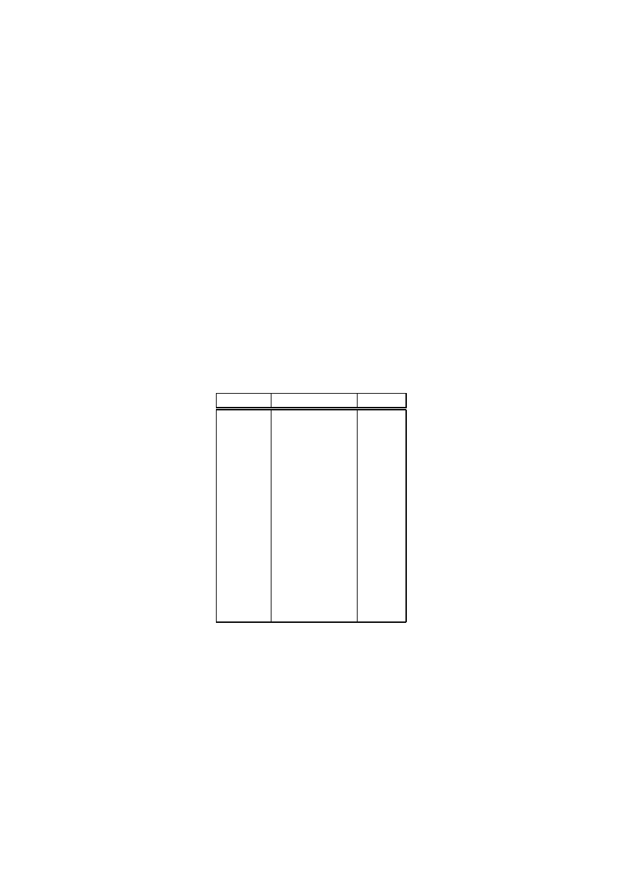
Appendix A
Symbol Table
In this appendix we present a table that summarises the meaning of each of
the special Haskell symbols that are used in this book, and shows how each of
the symbols is typed using a normal keyboard.
Symbol
Meaning
Typed
→
maps to
->
⇒
constrains
=>
at least
>=
at most
<=
=
inequality
/=
∧
conjunction
&&
∨
disjunction
||
¬
negation
not
↑
exponentiation
^
◦
composition
.
λ
abstraction
\
+
+
append
++
←
drawn from
<-
>
>=
bind
>>=
+++
choice
+++
107

c
Graham Hutton
Draft: not for distribution
108

Appendix B
Haskell Standard Prelude
In this appendix we present some of the most commonly used definitions from
the standard prelude. For clarity, a number of the definitions have been sim-
plified or modified from those given in the Haskell Report [11]. Other standard
libraries are described in the Haskell Library Report [10].
B.1
Classes
Equality types:
class Eq a where
(==), (
=)
:: a
→ a → Bool
x
= y
=
¬ (x == y)
Ordered types:
class Eq a
⇒ Ord a where
(<), (
), (>), ()
:: a
→ a → Bool
min, max
:: a
→ a → a
min x y
| x y
= x
| otherwise = y
max x y
| x y
= y
| otherwise = x
Showable types:
class Show a where
show
:: a
→ String
Readable types:
class Read a where
read
:: String
→ a
109

c
Graham Hutton
Draft: not for distribution
Numeric types:
class (Eq a, Show a)
⇒ Num a where
(+), (
−), (∗)
:: a
→ a → a
negate, abs, signum
:: a
→ a
Integral types:
class Num a
⇒ Integral a where
div , mod
:: a
→ a → a
Fractional types:
class Num a
⇒ Fractional a where
(/)
:: a
→ a → a
recip
:: a
→ a
recip n
= 1 / n
B.2
Booleans
Type declaration:
data Bool
= False
| True
deriving (Eq, Ord , Show , Read )
Logical conjunction:
(
∧)
:: Bool
→ Bool → Bool
False
∧
= False
True
∧ b
= b
Logical disjunction:
(
∨)
:: Bool
→ Bool → Bool
False
∨ b
= b
True
∨
= True
Logical negation:
¬
:: Bool
→ Bool
¬ False
= True
¬ True
= False
Guard that always succeeds:
otherwise
:: Bool
otherwise
= True
110

c
Graham Hutton
Draft: not for distribution
B.3
Characters and strings
Type declarations:
data Char
=
· · ·
deriving (Eq, Ord , Show , Read )
type String
= [Char ]
Decide if a character is a lower-case letter:
isLower
:: Char
→ Bool
isLower c
= c
’a’ ∧ c ’z’
Decide if a character is an upper-case letter:
isUpper
:: Char
→ Bool
isUpper c
= c
’A’ ∧ c ’Z’
Decide if a character is alphabetic:
isAlpha
:: Char
→ Bool
isAlpha c
= isLower c
∨ isUpper c
Decide if a character is a digit:
isDigit
:: Char
→ Bool
isDigit c
= c
’0’ ∧ c ’9’
Decide if a character alpha-numeric:
isAlphaNum
:: Char
→ Bool
isAlphaNum c
= isAlpha c
∨ isDigit c
Decide if a character is a spacing character:
isSpace
:: Char
→ Bool
isSpace c
= elem c "\t\n"
Convert a character to a Unicode number:
ord
:: Char
→ Int
ord
=
· · ·
Convert a Unicode number to a character:
chr
:: Int
→ Char
chr
=
· · ·
Convert a digit to an integer:
digitToInt
:: Char
→ Int
digitToInt c
| isDigit c = ord c − ord ’0’
111

c
Graham Hutton
Draft: not for distribution
Convert an integer to a digit:
intToDigit
:: Int
→ Char
intToDigit n
| n 0 ∧ n 9
= chr (ord ’0’ + n)
Convert a letter to lower-case:
toLower
:: Char
→ Char
toLower c
| isUpper c
= chr (ord c
− ord ’A’ + ord ’a’)
| otherwise
= c
Convert a letter to upper-case:
toUpper
:: Char
→ Char
toUpper c
| isLower c
= chr (ord c
− ord ’a’ + ord ’A’)
| otherwise
= c
B.4
Numbers
Type declarations:
data Int
=
· · ·
deriving (Eq, Ord , Show , Read ,
Num, Integral )
data Integer
=
· · ·
deriving (Eq, Ord , Show , Read ,
Num, Integral )
data Float
=
· · ·
deriving (Eq, Ord , Show , Read ,
Num, Fractional )
Decide if an integer is even:
even
:: Integral a
⇒ a → Bool
even n
= n ‘mod ‘ 2 == 0
Decide if an integer is odd:
odd
:: Integral a
⇒ a → Bool
odd
=
¬ ◦ even
Exponentiation:
(
↑)
:: (Num a, Integral b)
⇒ a → b → a
↑ 0
= 1
x
↑ (n + 1)
= x
∗ (x ↑ n)
112

c
Graham Hutton
Draft: not for distribution
B.5
Tuples
Type declarations:
data ()
=
· · ·
deriving (Eq, Ord , Show , Read )
data (a, b)
=
· · ·
deriving (Eq, Ord , Show , Read )
data (a, b, c)
=
· · ·
deriving (Eq, Ord , Show , Read )
..
.
Select the first component of a pair:
fst
:: (a, b)
→ a
fst (x , )
= x
Select the second component of a pair:
snd
:: (a, b)
→ b
snd ( , y)
= y
B.6
Lists
Type declaration:
data [a ]
= [ ]
| a : [a ]
deriving (Eq, Ord , Show , Read )
Decide if a list is empty:
null
:: [a ]
→ Bool
null [ ]
= True
null ( : )
= False
Decide if a value is an element of a list:
elem
:: Eq a
⇒ a → [a ] → Bool
elem x xs
= any (== x ) xs
Decide if all logical values in a list are True:
and
:: [Bool ]
→ Bool
and
= foldr (
∧) True
Decide if any logical value in a list is False:
or
:: [Bool ]
→ Bool
or
= foldr (
∨) False
Decide if all elements of a list satisfy a predicate:
113

c
Graham Hutton
Draft: not for distribution
all
:: (a
→ Bool) → [a ] → Bool
all p
= and
◦ map p
Decide if any element of a list satisfies a predicate:
any
:: (a
→ Bool) → [a ] → Bool
any p
= or
◦ map p
Select the first element of a non-empty list:
head
:: [a ]
→ a
head (x : )
= x
Select the last element of a non-empty list:
last
:: [a ]
→ a
last [x ]
= x
last ( : xs)
= last xs
Select the nth element of a list:
(!!)
:: [a ]
→ Int → a
(x : ) !! 0
= x
( : xs) !! (n + 1)
= xs !! n
Select the first n elements of a list:
take
:: Int
→ [a ] → [a ]
take 0
= [ ]
take (n + 1) [ ]
= [ ]
take (n + 1) (x : xs)
= x : take n xs
Select all elements of a list that satisfy a predicate:
filter
:: (a
→ Bool) → [a ] → [a ]
filter p xs
= [x
| x ← xs, p x ]
Select elements of a list while they satisfy a predicate:
takeWhile
:: (a
→ Bool) → [a ] → [a ]
takeWhile
[ ]
= [ ]
takeWhile p (x : xs)
| p x
= x : takeWhile p xs
| otherwise
= [ ]
Remove the first element from a non-empty list:
tail
:: [a ]
→ [a ]
tail ( : xs)
= xs
Remove the last element from a non-empty list:
114

c
Graham Hutton
Draft: not for distribution
init
:: [a ]
→ [a ]
init [ ]
= [ ]
init (x : xs)
= x : init xs
Remove the first n elements from a list:
drop
:: Int
→ [a ] → [a ]
drop 0 xs
= xs
drop (n + 1) [ ]
= [ ]
drop (n + 1) ( : xs)
= drop n xs
Remove elements from a list while they satisfy a predicate:
dropWhile
:: (a
→ Bool) → [a ] → [a ]
dropWhile
[ ]
= [ ]
dropWhile p (x : xs)
| p x
= dropWhile p xs
| otherwise
= x : xs
Split a list at the nth element:
splitAt
:: Int
→ [a ] → ([a ], [a ])
splitAt n xs
= (take n xs, drop n xs)
Split a list using a predicate:
span
:: (a
→ Bool) → [a ] → ([a ], [a ])
span p xs
= (takeWhile p xs, dropWhile p xs)
Process a list using a right-bracketing function:
foldr
:: (a
→ b → b) → b → [a ] → b
foldr
v [ ]
= v
foldr f v (x : xs)
= f x (foldr f v xs)
Process a non-empty list using a right-bracketing function:
foldr1
:: (a
→ a → a) → [a ] → a
foldr1
[x ]
= x
foldr1 f (x : xs)
= f x (foldr1 f xs)
Process a list using a left-bracketing function:
foldl
:: (a
→ b → a) → a → [b ] → a
foldl
v [ ]
= v
foldl f v (x : xs)
= foldl f (f v x ) xs
Process a non-empty list using a left-bracketing function:
foldl1
:: (a
→ a → a) → [a ] → a
foldl1 f (x : xs)
= foldl f x xs
Produce an infinite list of identical elements:
115

c
Graham Hutton
Draft: not for distribution
repeat
:: a
→ [a ]
repeat x
= xs where xs = x : xs
Produce a list with n identical elements:
replicate
:: Int
→ a → [a ]
replicate n
= take n
◦ repeat
Produce an infinite list by iterating a function over a value:
iterate
:: (a
→ a) → a → [a ]
iterate f x
= x : iterate f (f x )
Produce a list of pairs from a pair of lists:
zip
:: [a ]
→ [b ] → [(a, b)]
zip [ ]
= [ ]
zip
[ ]
= [ ]
zip (x : xs) (y : ys)
= (x , y) : zip xs ys
Calculate the length of a list:
length
:: [a ]
→ Int
length [ ]
= 0
length ( : xs)
= 1 + length xs
Calculate the sum of a list of numbers:
sum
:: Num a
⇒ [a ] → a
sum
= foldl (+) 0
Calculate the product of a list of numbers:
product
:: Num a
⇒ [a ] → a
product
= foldl (
∗) 1
Calculate the minimum of a non-empty list:
minimum
:: Ord a
⇒ [a ] → a
minimum
= foldl1 min
Calculate the maximum of a non-empty list:
maximum
:: Ord a
⇒ [a ] → a
maximum
= foldl1 max
Append two lists:
(+
+)
:: [a ]
→ [a ] → [a ]
[ ] +
+ ys
= ys
(x : xs) +
+ ys
= x : (xs +
+ ys)
Concatenate a list of lists:
116

c
Graham Hutton
Draft: not for distribution
concat
:: [[a ]]
→ [a ]
concat
= foldr (+
+) [ ]
Reverse a list:
reverse
:: [a ]
→ [a ]
reverse
= foldl (λxs x
→ x : xs) [ ]
Apply a function to all elements of a list:
map
:: (a
→ b) → [a ] → [b ]
map f xs
= [f x
| x ← xs ]
B.7
Functions
Type declaration:
data a
→ b
=
· · ·
Identity function:
id
:: a
→ a
id
= λx
→ x
Function composition:
(
◦)
:: (b
→ c) → (a → b) → (a → c)
f
◦ g
= λx
→ f (g x)
Constant functions:
const
:: a
→ (b → a)
const x
= λ
→ x
Convert a function on pairs to a curried function:
curry
:: ((a, b)
→ c) → (a → b → c)
curry f
= λx y
→ f (x, y)
Convert a curried function to a function on pairs:
uncurry
:: (a
→ b → c) → ((a, b) → c)
uncurry f
= λ(x , y)
→ f x y
B.8
Actions
Type declaration:
data IO a
=
· · ·
Read a character from the keyboard:
117

c
Graham Hutton
Draft: not for distribution
getChar
::
IO Char
getChar
=
· · ·
Read a string from the keyboard:
getLine
::
IO String
getLine
=
do x
← getChar
if x == ’\n’ then
return ""
else
do xs
← getLine
return (x : xs)
Read a value from the keyboard:
readLn
::
Read a
⇒ IO a
readLn
=
do xs
← getLine
return (read xs)
Write a character to the screen:
putChar
::
Char
→ IO ()
putChar
=
· · ·
Write a string to the screen:
putStr
::
String
→ IO ()
putStr ""
=
return ()
putStr (x : xs)
=
do putChar x
putStr xs
Write a string to the screen and move to a new line:
putStrLn
::
String
→ IO ()
putStrLn xs
=
do putStr xs
putChar ’\n’
Write a value to the screen:
::
Show a
⇒ a → IO ()
=
putStrLn
◦ show
Display an error message and terminate evaluation:
error
::
String
→ a
error
=
· · ·
118
Wyszukiwarka
Podobne podstrony:
developerWorks Tutorial XML programming in Java (1999)
Call for Applications HIA Program in US 09
Examples of Programming in Matlab (2001) WW
Practical Artificial Intelligence Programming in Java
concurrent programming in mac os x and ios
Portable Programming in C (2)
European transnational ecological deprivation index and index and participation in beast cancer scre
(ebook pdf) programming primer for object oriented and procedural programming in java, c, c
Heather Graham Strangers In Paradise
Teffaha D Relevance of Water Gymnastics in Rehabilitation Programs in
Concurrent Programming in Erlan Part 1
Podstawa programowa katechezy w przedszkolu m.in. zerwka, Bałagan - czas posprzątać i poukładać
Basic Microcontroller in C Programming
BYT 2004 Roles in programming project
więcej podobnych podstron