•

1

•

1

B

ASIC

F

IBONACCI

P

RINCIPLES

“Let your imagination soar.” This phrase, this invitation, started the
earlier book, Fibonacci Applications and Strategies for Traders. And
once again, we do not hesitate to introduce readers to the fascination
of the f indings of Leonardo Di Pisa, commonly known as Fibonacci,
by publishing this renewed appeal to creativity and imagination.

Eight years have passed since Fibonacci Applications and Strate-

gies for Traders was published. The market environment has changed
a great deal. What has remained unchanged, however, is the beauty of
nature. Think of all the wonders of nature in our world: oceans, trees,
f lowers, plant life, animals, and microorganisms.

Also think of the achievements of humans in natural sciences,

nuclear theory, medicine, computer technology, radio, and television.
And f inally, think of the trend moves in world markets. It may sur-
prise you to learn that all of these have one underlying pattern in com-
mon: the Fibonacci summation series.

The Fibonacci summation series, the baseline of our pattern-

oriented market analysis, is presented in this f irst chapter. After the
meaning of this sequence of numbers has become clear, we take a
quick look at the types of phenomena and achievements in human

fisc_c01.qxd 8/22/01 8:38 AM Page 1

2

•

BASIC FIBONACCI PRINCIPLES

behavior that can be analyzed using the Fibonacci summation series.
We then point out the conclusions drawn by engineer and trader Ralph
Nelson Elliott. We look at the generalizations he made to provide an-
alysts today with a nonstringent framework that can be used for the
sake of prof itable trading in global markets.

Chapter 1 is designed as a recap of Fibonacci Applications and

Strategies for Traders. Readers who are familiar with the details of
Fibonacci and Elliott in this f irst chapter may want to proceed to the
overview of what is new in this book, on page 22.

THE FIBONACCI SUMMATION SERIES

Fibonacci (1170–1240) lived and worked as a merchant and mathe-
matician in Pisa, Italy. He was one of the most illustrious European
scientists of his time. Among his greatest achievements was the in-
troduction of Arabic numerals to supersede the Roman f igures.

He developed the Fibonacci summation series, which runs as

or, in mathematical terms,

The mathematical series tends asymptotically (that is, ap-

proaching slower and slower) toward a constant ratio.

However, this ratio is irrational; it has a never-ending, unpre-

dictable sequence of decimal values stringing after it. It can never be
expressed exactly. If each number, as part of the series, is divided by
its preceding value (e.g., 13 ÷ 8 or 21 ÷ 13), the operation results in a
ratio that oscillates around the irrational f igure 1.61803398875 . . . ,
being higher than the ratio one time, and lower the next. The precise
ratio will never, into eternity (not even with the most powerful com-
puters developed in our age), be known to the last digit. For the sake of
brevity, we will refer to the Fibonacci ratio as 1.618 and ask readers to
keep the margin of error in mind.

This ratio had begun to gather special names even before another

medieval mathematician, Luca Pacioli (1445–1514), named it “the divine
proportion.” Among its contemporary names are “golden section” and
“golden mean.” Johannes Kepler (1571–1630), a German astronomer,

a

a

a

a

a

n

n

n

+

−

=

+

=

=

1

1

1

2

1

with

1 1

2

3

5

8 13 21 34 55 89 144

– –

–

–

–

–

–

–

–

–

–

– . . .

fisc_c01.qxd 8/22/01 8:38 AM Page 2

THE FIBONACCI SUMMATION SERIES

•

3

called the Fibonacci ratio one of the jewels in geometry. Algebraically,
it is generally designated by the Greek letter PHI (

ϕ), with

or, in a different mathematical form

And it is not only PHI that is interesting to scientists (and

traders, as we shall see). If we divide any number of the Fibonacci
summation series by the number that follows it in the series (e.g., 8 ÷
13 or 13 ÷ 21), we f ind that the series asymptotically gets closer to
the ratio PHI

′ with

being simply the reciprocal value to PHI with

or, in another form,

This is a very unusual and remarkable phenomenon—and a use-

ful one when it comes to designing trading tools, as we will learn in
the course of the analysis. Because the original ratio PHI is irrational,
the reciprocal value PHI

′ to the ratio PHI necessarily turns out to be

an irrational f igure as well, which means that we again have to con-
sider a slight margin of error when calculating 0.618 in an approxi-
mated, shortened way.

From here on, we analytically exploit PHI and PHI

′ and move

ahead by slightly reformulating the Fibonacci summation series so
that the following PHI series is the result:

In mathematical terms, it is written as

a

a

a

a

a

n

n

n

+

−

=

+

=

=

1

1

1

2

0 618

1

with .

,

0 618 1 000 1 618 2 618

4 236 6 854 11 090 17 944

.

.

.

.

.

.

.

.

. . .

−

−

−

−

−

−

−

−

′ =

−

(

)

≈

ϕ

1

2

5

1

0 618

.

′ =

÷ = ÷

≈

ϕ

ϕ

1

1 1 618

0 618

.

.

′ ≈

ϕ

0 618

.

ϕ =

+

(

)

≈

1

2

5

1

1 618

.

ϕ ≈ 1 618

.

fisc_c01.qxd 8/22/01 8:38 AM Page 3

4

•

BASIC FIBONACCI PRINCIPLES

In this case, we do not f ind an asymptotical process with a ratio

because, in dividing each number of the PHI series by its preceding
value (e.g., 4.236 ÷ 2.618 or 6.854 ÷ 4.236), the operation results in
the approximated ratio PHI

= 1.618. Running the division in the op-

posite direction—that is, dividing each number of the PHI series by
the value that follows (e.g., 2.618 ÷ 4.236 or 4.236 ÷ 6.854)—results
in the reciprocal value to the constant PHI, introduced earlier as
PHI

′ = 0.618. Before progressing further through the text, it is im-

portant that readers fully understand how the PHI series has been
derived from the underlying Fibonacci summation series.

We have discovered a series of plain figures, applied to science by

Fibonacci. We must take another quick detour before we can utilize
the Fibonacci summation series as the basis for the development of
trading tools. We must f irst consider what relevance the Fibonacci
summation series has for nature around us. It will then be only a
small step to conclusions that lead us directly to the relevance of the
Fibonacci summation series for the movement of international mar-
kets, whether in currencies or commodities, stocks or derivatives.

We recognize the dampened swings of the quotients around the

value of 1.618 (or 0.618, respectively) in Fibonacci’s series by either
higher or lower numbers in the Elliott wave principle, which was pop-
ularized by Ralph Nelson Elliott as the rule of alternation. And we
present the trading tools that we developed for exploration of the magic
of PHI to the largest extent possible. Humans subconsciously seek the
divine proportion, which is nothing but a constant and timeless striv-
ing to create a comfortable standard of living.

THE FIBONACCI RATIO

For us—and, hopefully, for our readers as well—it remains remark-
able how many constant values can be calculated using Fibonacci’s se-
quence, and how the individual f igures that form the sequence recur
in so many variations. However, it cannot be stressed strongly enough
that this is not just a numbers game; it is the most important mathe-
matical representation of natural phenomena ever discovered. The
following illustrations depict some interesting applications of this
mathematical sequence.

We have subdivided our observations into two sections. First,

we deal brief ly with the Fibonacci ratio and its presence in natural

fisc_c01.qxd 8/22/01 8:38 AM Page 4

THE FIBONACCI RATIO

•

5

phenomena and in architecture. Then we brief ly describe how math-
ematics, physics, and astronomy make use of the Fibonacci ratio.

The Fibonacci Ratio in Nature

To appreciate the great relevance of the Fibonacci ratio as a natural
constant, one need only look at the beauty of nature that surrounds us.
The development of plants in nature is a perfect example of the gen-
eral relevance of the Fibonacci ratio and the underlying Fibonacci
summation series. Fibonacci numbers can be found in the number of
axils on the stem of every growing plant, as well as in the number
of petals.

We can easily f igure out member numbers of the Fibonacci sum-

mation series in plant life (so-called golden numbers) if we count the
petals of certain common f lowers—for example, the iris with 3 petals,
the primrose with 5 petals, the ragwort with 13 petals, the daisy with
34 petals, and the Michaelmas daisy with 55 (and 89) petals. We must
question: Is this pattern accidental or have we identif ied a particular
natural law?

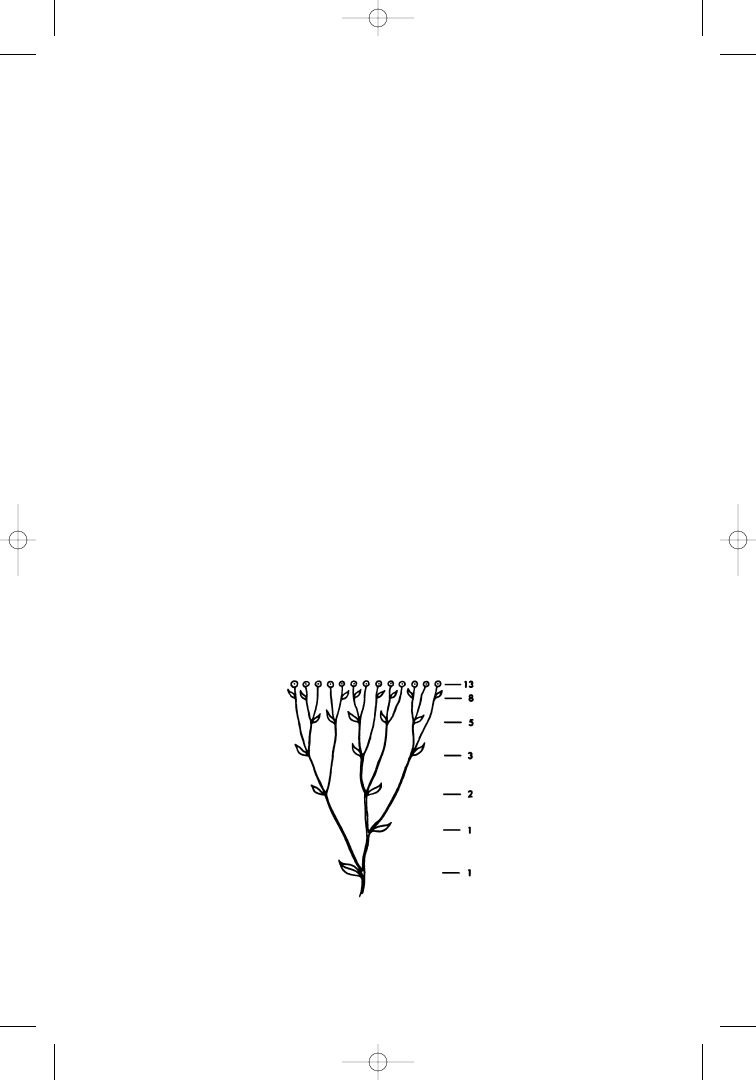
An ideal example is found in the stems and f lowers of the sneeze-

wort (Figure 1.1). Every new branch of sneezewort springs from the
axil, and more branches grow from a new branch. Adding the old and
the new branches together, a Fibonacci number is found in each hori-
zontal plane.

Figure 1.1

Fibonacci numbers found in the flowers of the sneezewort.

fisc_c01.qxd 8/22/01 8:38 AM Page 5

6

•

BASIC FIBONACCI PRINCIPLES

When analyzing world markets and developing trading strate-

gies, we look for structures or chart patterns that have been prof-
itable in the past (according to historical data) and therefore shall
have a probability of continued success in the future. In the Fi-
bonacci ratio PHI, we propose to have found such a structure or gen-
eral pattern.

The Fibonacci ratio PHI is an irrational f igure. We will never

know its exact value to the last digit. Because the error margin ap-
proximating the Fibonacci ratio PHI gets smaller as the numbers of
the Fibonacci summation series become higher, we consider 8 the
smallest of all the numbers of the Fibonacci summation series that
can be meaningfully applied to market analysis (calculating the sam-
ple quotients of 13 ÷ 8

= 1.625 and 21 ÷ 13 = 1.615, compared with

PHI

= 1.618).

At different times and on different continents, people have at-

tempted to successfully incorporate the ratio PHI into their work as
a law of perfect proportion. Not only were the Egyptian pyramids
built according to the Fibonacci ratio PHI (as described in detail in
Fibonacci Applications and Strategies for Traders), but the same phe-
nomenon can be found in the Mexican pyramids.

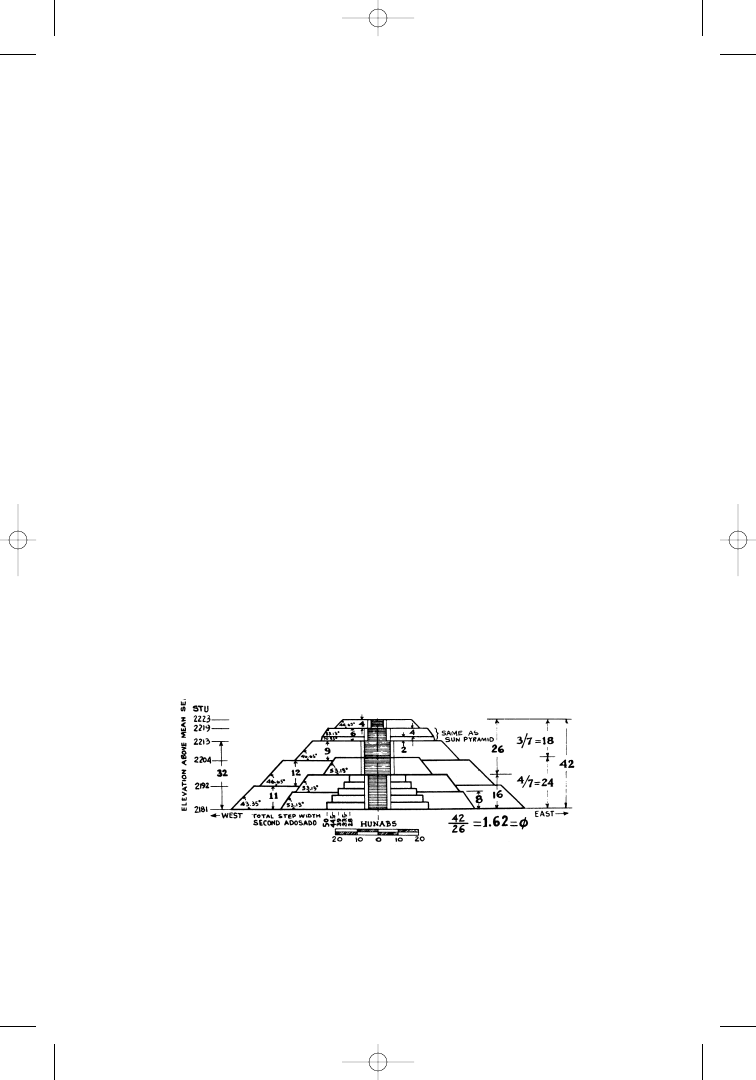
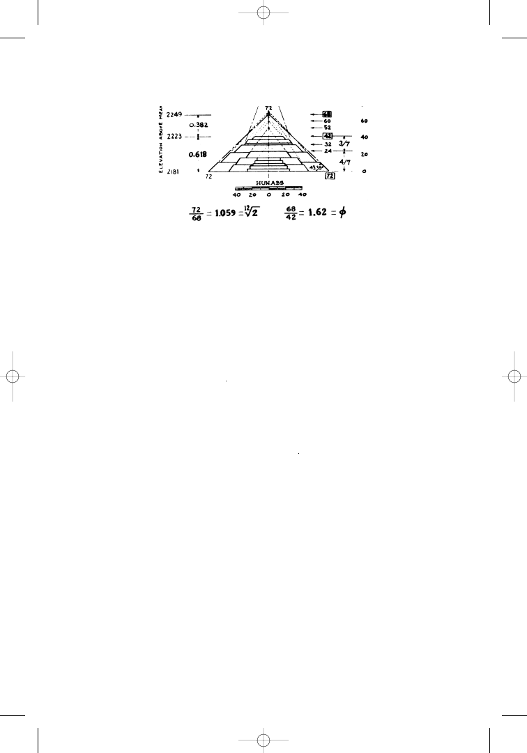
It is conceivable that the Egyptian and the Mexican pyramids

were built in approximately the same historical era by people of com-
mon origins. Figure 1.2a and Figure 1.2b illustrate the importance of
the incorporated Fibonacci proportion PHI.

Figure 1.2a

Number PHI

= 1.618 incorporated in the Mexican pyramid.

Source: Mysteries of the Mexican Pyramid, by Peter Thomkins (New York:
Harper & Row, 1976), pp. 246, 247. Reprinted with permission.

fisc_c01.qxd 8/22/01 8:38 AM Page 6

THE FIBONACCI RATIO

•

7

A cross-section of the pyramid shows a structure shaped as a

staircase. There are 16 steps in the f irst set, 42 steps in the second,
and another 68 steps in the third. These numbers are based on the
Fibonacci ratio 1.618 in the following way:

Here we f ind (although not at f irst glance) Fibonacci’s ratio PHI

in a macrostructure familiar to all of us. Our task is to transfer this
approach from nature and the human environment to the sphere of
chart and market analysis. In our market environment, we must ask
whether and where we can detect PHI as purely and exploitably as in
natural plant life and manmade pyramids.

The Fibonacci Ratio in Geometry

The existence of the Fibonacci ratio PHI in geometry is also very well
known. However, a workable way for investors to apply this ratio, as
a geometric tool, to commodity price moves using PHI-spirals and

16 1 618

26

16 26

42

26 1 618

42

26

42

68

42 1 618

68

×

=

+

=

×

=

+

=

×

=

.

.

.

Figure 1.2b

Number PHI

= 1.618 incorporated in the Mexican pyramid.

Source: Mysteries of the Mexican Pyramid, by Peter Thomkins (New York:
Harper & Row, 1976), pp. 246, 247. Reprinted with permission.

fisc_c01.qxd 8/22/01 8:38 AM Page 7

8

•

BASIC FIBONACCI PRINCIPLES

PHI-ellipses has not yet been published. It takes a programmer’s
knowledge and the power of computers to apply the PHI-spiral and
the PHI-ellipse as analytic tools.

Because computer power is easily accessible today, the obstacle

is not the hardware, but rather some missing knowledge and the lack
of appropriate software.

The fully operational software package that accompanies this

book allows every interested reader/investor to trace the examples
shown and to generate similar signals in real-time trading.

PHI-spiral and PHI-ellipse consist of unusual properties that are

in accordance with Fibonacci’s ratio PHI in two dimensions: price and
time. It is very likely that the integration of PHI-spirals and PHI-
ellipses will elevate the interpretation and the use of the Fibonacci
ratio to a much higher level. Up to now, Fibonacci’s PHI has been gen-
erally accepted as a tool for the measurement of corrections and ex-
tensions of price swings. Forecasts of time have seldom been
integrated because they did not seem to be as reliable as the price
analysis, but, by including PHI-spirals and PHI-ellipses into a geo-
metric analysis, both parts—price and time analyses—can be com-
bined accurately.

To gain a better understanding of how Fibonacci’s PHI is geo-

metrically incorporated into PHI-spirals and PHI-ellipses, we begin by
describing the golden section of a line and of a rectangle, and their
respective relations to PHI.

A Greek mathematician, Euclid of Megara (450–370

B

.

C

.), was

the f irst scientist to write about the golden section and thereby fo-
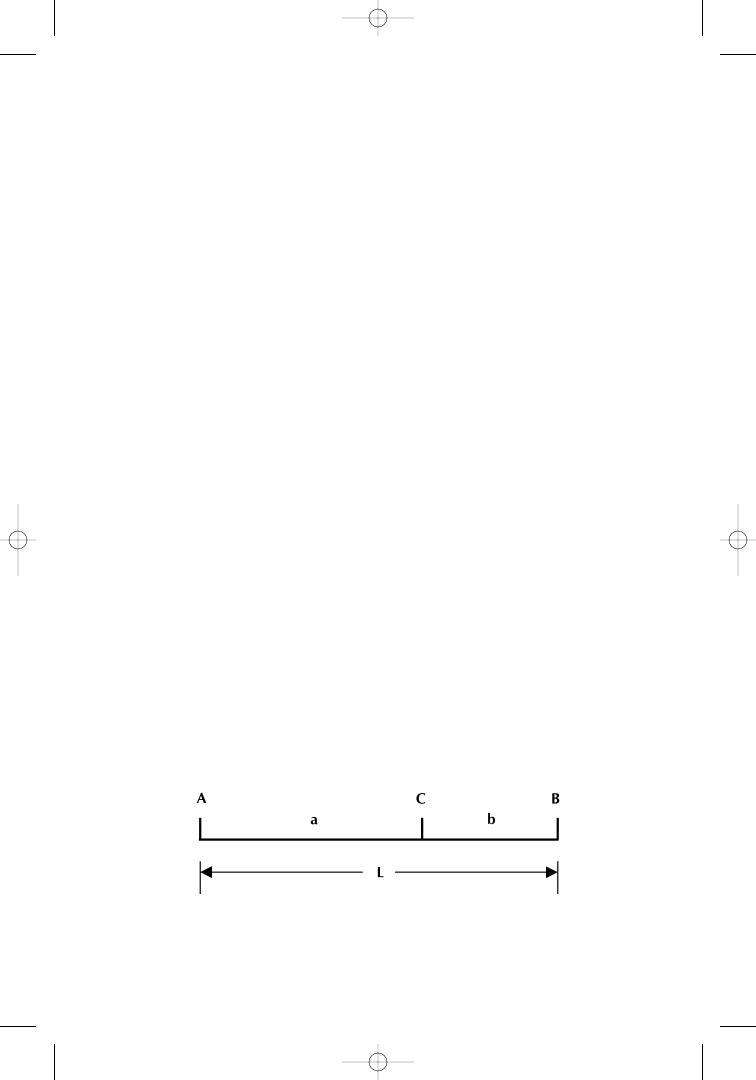
cused on the analysis of a straight line (Figure 1.3).

The line AB of length L is divided into two segments by point C.

Let the length of AC and CB be a and b, respectively. If C is a point

Figure 1.3

Golden section of a line. Source: FAM Research, 2000.

fisc_c01.qxd 8/22/01 8:38 AM Page 8

THE FIBONACCI RATIO

•

9

such that the quotient L ÷ a equals a ÷ b, then C is the golden section
of AB. The ratio L ÷ a or a ÷ b is called the golden ratio.

In other words, point C divides the line AB into two parts in such

a way that the ratios of those parts are 1.618 and 0.618; two f igures
we easily recognize from our analysis of the Fibonacci summation
series as Fibonacci’s PHI and its reciprocal value PHI

′.

Moving from one cradle of science to another—from ancient Eu-

rope to ancient Africa, or from ancient Greece to ancient Egypt—we
learn that in the Great Pyramid of Gizeh, the rectangular f loor of the
king ’s chamber also illustrates the golden section.

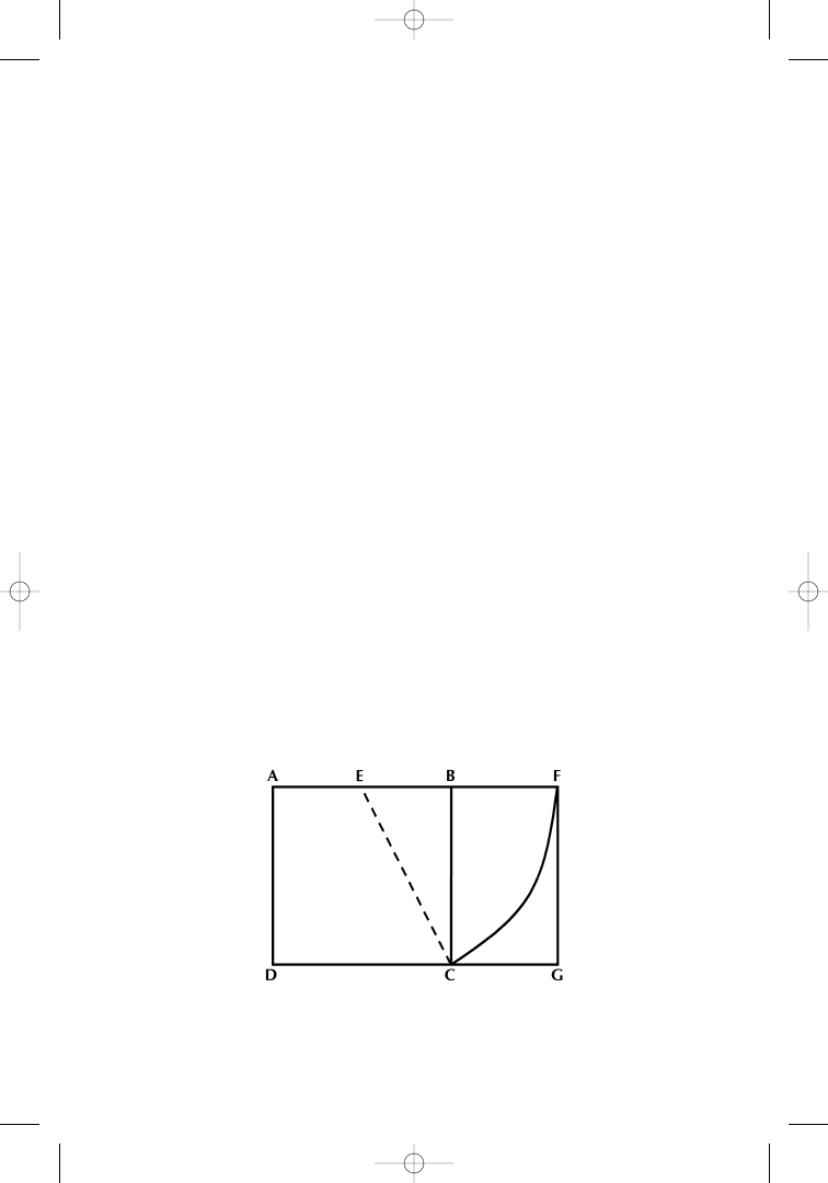
The golden section of a rectangle can best be demonstrated by

starting with a square, a geometrical formation that served as the
foundation for the Pyramid of Gizeh. This square can then be trans-
formed into a golden rectangle as has been done schematically in Fig-
ure 1.4.

Side AB of the square ABCD in Figure 1.4 is bisected. With the

center E and the radius EC, an arc of a circle is drawn, cutting the ex-
tension of AB at F. Line FG is drawn perpendicular to AF, meeting
the extension of DC at G. AFGD is the golden rectangle. According to
the formal definition, the geometrical representation of the golden sec-
tion in a rectangle means that a rectangle of this form is 1.618 times
longer than it is wide. Again, Fibonacci’s ratio PHI appears, this time
in the proportions of the golden rectangle.

Keeping in mind the representation of the Fibonacci ratio PHI in

one-dimensional (line) and two-dimensional (rectangle) geometry, we
can proceed to more complex geometrical objects that bring us closer

Figure 1.4

Golden section of a rectangle. Source: FAM Research, 2000.

fisc_c01.qxd 8/22/01 8:38 AM Page 9

10

•

BASIC FIBONACCI PRINCIPLES

to the tools we want to apply to analyze stock and commodity markets
with regard to time and price.

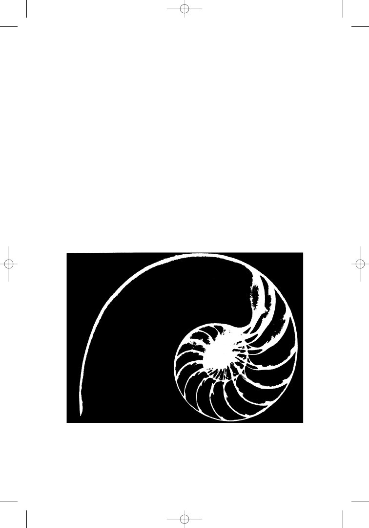
The only mathematical curve that follows the pattern of natural

growth is the spiral, expressed in natural phenomena such as Spira
mirabilis, or the nautilus shell. The PHI-spiral has been called the
most beautiful of mathematical curves. This type of spiral occurs fre-
quently in the natural world. The Fibonacci summation series and the
golden section, introduced above as its geometrical equivalent, are
very well associated with this remarkable curve.

Figure 1.5 shows a radiograph of the shell of the chambered nau-

tilus. The successive chambers of the nautilus are built on the frame-
work of a PHI-spiral. As the shell grows, the size of the chambers
increases, but their shape remains unaltered.

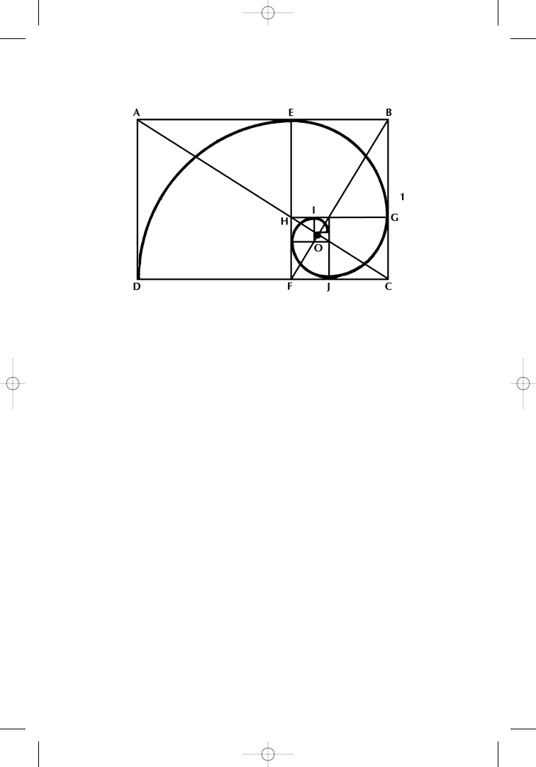
To demonstrate the geometry of the PHI-spiral, it is best to use

a golden rectangle as the basis for geometrical analysis. This is done
schematically in Figure 1.6.

Figure 1.5

The PHI-spiral represented in the nautilus shell. Source: The Divine

Proportion, by H. E. Huntley (New York: Dover, 1970), p. iv. Reprinted with
permission.

fisc_c01.qxd 8/22/01 8:38 AM Page 10

THE FIBONACCI RATIO

•

11

The quotient of the length and height of rectangle ABCD in Fig-

ure 1.6 can be calculated, as we learned previously, by AB ÷ BC

= PHI

÷ 1

= 1.618. Through point E, also called the golden cut of AB, line EF

is drawn perpendicular to AB, cutting the square AEFD from the rec-
tangle. The remaining rectangle EBCF is a golden rectangle. If the
square EBGH is isolated, the then remaining f igure, HGCF, is also a
golden rectangle. This process can be repeated indef initely until the
limiting rectangle O is so small that it is indistinguishable from
a point.

The limiting point O is called the pole of the equal angle spiral,

which passes through the golden cuts D, E, G, J, and so on. The
sides of the rectangle are nearly, but not completely, tangential to
the curve.

The relation of the PHI-spiral to the Fibonacci series is evident

from Figure 1.6 because the PHI-spiral passes diagonally through
opposite corners of successive squares, such as DE, EG, GJ, and so
on. The lengths of the sides of these squares form a Fibonacci series.
If the smallest square has a side of length d, the adjacent square
must also have a side of length d. The next square has a side of
length 2d (twice as long as d), the next of 3d (three times the length
of d), forming the series 1d, 2d, 3d, 5d, 8d, 13d, . . . which is exactly

Figure 1.6

Geometry of the PHI-spiral. Source: FAM Research, 2000.

fisc_c01.qxd 8/22/01 8:38 AM Page 11

12

•

BASIC FIBONACCI PRINCIPLES

the well-known Fibonacci sequence: 1–1–2–3–5–8–13– and so on,
indef initely.

The spiral is without a terminal point. While growing outward

(or inward) indef initely, its shape remains unchanged. Two segments
of the spiral are identical in shape, but they differ in size by exactly
the factor PHI. All those spirals whose rate of growth is an element of
the PHI series 0.618–1.000–1.618–2.618–4.236– 6.854–11.090– and
so on, shall be referred to as PHI-spirals in the context of this book.

The PHI-spiral is the link between the Fibonacci summation se-

ries, the resulting Fibonacci ratio PHI, and the magic of nature that
we enjoy all around us.

In addition to the PHI-spiral, other important geometric curves

can be found in nature. Those most signif icant to civilization include
the horizon of the ocean, the meteor track, the parabola of a waterfall,
the arc the sun travels, the crescent moon, and, f inally, the f light of a
bird. Many of these natural curves can be geometrically modeled using
ellipses.

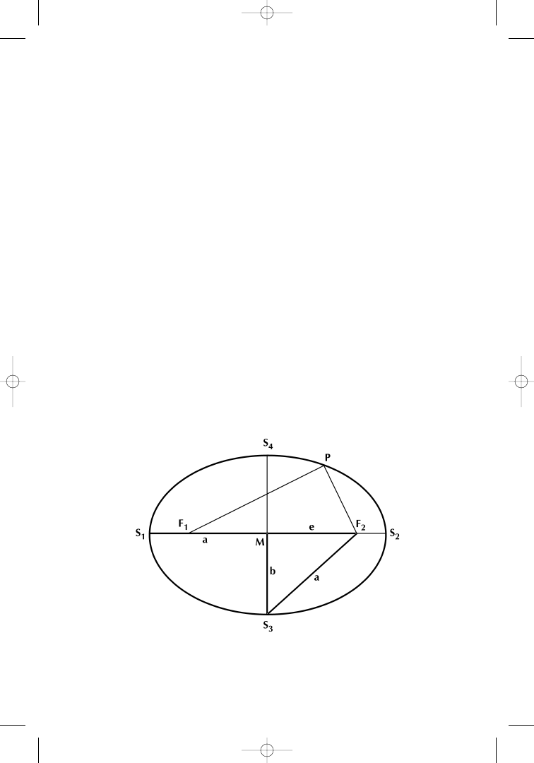
An ellipse is the mathematical expression of an oval. Each el-

lipse can be precisely designated by only a few characteristics (Fig-
ure 1.7).

Figure 1.7

Geometry of the PHI-ellipse. Source: FAM Research, 2000.

fisc_c01.qxd 8/22/01 8:38 AM Page 12

THE FIBONACCI RATIO

•

13

S

1

S

2

in Figure 1.7 represents the length of the major axis of the

ellipse. S

3

S

4

is the length of the minor axis of the ellipse. The ellipse

is now determined by the equation

Of interest to us, in the context of Fibonacci analysis, is the ratio

of the major axis and minor axis of the ellipse, in mathematical terms

An ellipse is turned into a PHI-ellipse in all those cases where

the ratio of the major axis to the minor axis of the ellipse is a mem-
ber number of the PHI series 0.618–1.000–1.618–2.618–4.236–
6.854– and so on. A circle is a special type of PHI-ellipse, with a

= b

and a ratio of a ÷ b

= 1.

What makes PHI-ellipses preferable to all other possible ellipses

(those with ratios of major axes divided by minor axes other than num-
bers of the PHI series) is the fact that empirical research has shown
that people f ind approximations of PHI-ellipses signif icantly more vi-
sually satisfying.

When participants in a research project were confronted with

different shapes of ellipses and were asked for their levels of comfort,
a sample empirical study returned the results shown in Table 1.1.

S S

S S

a

b

a

b

1

2

3

4

2

2

÷

=

÷

= ÷

F P

F P

S S

a

1

2

1

2

2

+

=

=

Table 1.1

Preferences for PHI-Ellipses

Ratio

Major Axis

÷ Minor Axis

Percentage of

a

÷ b

Preference

1.000

1.2

1.205

0.6

1.250

8.3

1.333

14.7

1.493

42.4

1.618

16.7

1.754

13.1

2.000

1.6

Source: The Divine Proportion, by H. E. Huntley (New York:
Dover, 1970) p. 65. Reprinted with permission.

fisc_c01.qxd 8/22/01 8:38 AM Page 13

14

•

BASIC FIBONACCI PRINCIPLES

Three observers out of four favored ellipses shaped with axes

whose ratios were either the PHI-ellipse (1.618) or so close an
approximation to the PHI-ellipse as to be almost indistinguishable
from it.

With this optimistic outlook, we can proceed to the second main

part of our theoretical introduction of basic Fibonacci tools.

What conclusions can be drawn from our discussions so far? And

what sort of conclusions did Elliott draw to integrate the Fibonacci
summation series and Fibonacci’s PHI with the forces that move in-
ternational markets?

THE ELLIOTT WAVE PRINCIPLE

Ralph Nelson Elliott (1871–1948) began his career as an engineer,
not a professional market analyst. Having recovered from a serious
illness in the 1930s, he turned his interest to the analysis of stock
prices, focusing on the Dow Jones Index.

After a number of remarkably successful forecasts, in 1939 El-

liott published a series of major articles in Financial World magazine.
In these articles, he f irst presented the contention that the Dow Jones
Index moved in rhythms.

Elliott’s market theory was based on the fact that every phe-

nomenon on our planet moves in the same patterns as the tides: low
tide follows high tide, reaction follows action. Time does not affect this
scheme because the structure of the market in its entirety remains
constant.

In this section, we brief ly review and analyze Elliott’s concepts.

However, it is important that we address his ideas, because they ex-
plain the fundamental concepts that we have used in our analysis of
the Fibonacci tools. We will not go into great detail here; most of the
facts have been discussed extensively in Fibonacci Applications and
Strategies for Traders.

Our attention will focus on the main sectors of Elliott’s work,

which have long-lasting value. Even if we do not agree with some of
Elliott’s f indings, he must be admired for his ideas. We know how dif-
f icult it was to create new concepts for market analysis without the
technical support that is available today. When we began to study
Elliott’s work, back in 1977, it was a tremendous struggle to get the

fisc_c01.qxd 8/22/01 8:38 AM Page 14

THE ELLIOTT WAVE PRINCIPLE

•

15

data needed for an in-depth analysis. How much more diff icult it must
have been for Elliott in those years when he started his work! The
computer technology available today gives us the ability to test and
analyze quickly, but it is still necessary to have Elliott’s ideas handy
in order to begin.

Elliott wrote: “Nature’s law embraces the most important of all

elements, timing. Nature’s law is not a system, or a method of play-
ing the market, but it is a phenomenon which appears to mark the
progress of all human activities. Its application to forecasting is
revolutionary.”*

Elliott based his discoveries on nature’s law. He noted: “This law

behind the market can only be discovered when the market is viewed
in its proper light and then is analyzed from this approach. Simply
put, the stock market is a creation of man and therefore ref lects
human idiosyncrasy” (p. 40).

The chance to forecast price moves using Elliott’s principles mo-

tivated legions of analysts to work day and night. We will focus on the
ability to forecast, and try to answer whether it is possible.

Elliott was very specific when he introduced his concept of waves.

He said: “All human activities have three distinctive features, pat-
tern, time and ratio, all of which observe the Fibonacci summation se-
ries” (p. 48).

Once the waves are interpreted, that knowledge may be applied

to any movement because the same rules apply to the prices of stocks,
bonds, grains, and other commodities.

The most important of the three factors mentioned is pattern. A

pattern is always in progress, forming over and over again. Usually,
but not invariably, one can visualize in advance the appropriate type
of pattern. Elliott describes this market cycle as “. . . divided primar-
ily into ‘bull market’ and ‘bear market’ ” (p. 48).

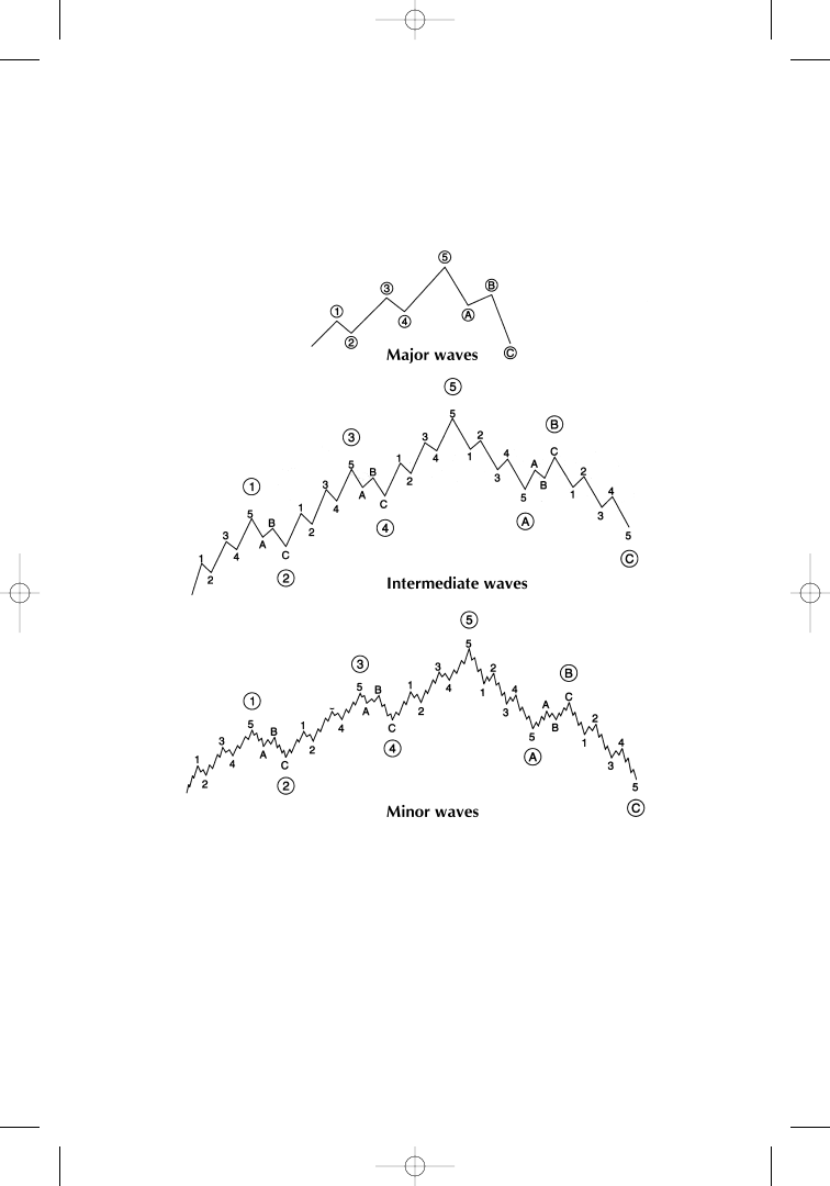
A bull market can be divided into f ive “major waves,” and a bear

market, into three major waves. The major waves 1, 3, and 5 of the
bull market are subdivided into f ive “intermediate waves” each. Then

* The Complete Writings of R. N. Elliott with Practical Application from J. R. Hill,
by J. R. Hill, Commodity Research Institute, NC, 1979 (subsequent references will
cite Elliott), p. 84.

fisc_c01.qxd 8/22/01 8:38 AM Page 15

16

•

BASIC FIBONACCI PRINCIPLES

waves 1, 3, and 5 of each intermediate wave are subdivided into f ive
“minor waves” (Figure 1.8).

The problem with this general market concept is that, most of the

time, there are no regular 5-wave swings. The regular 5-wave swing is
only the exception to a rule that Elliott tried to f ine-tune via a so-
phisticated variation to the concept.

Figure 1.8

Elliott ’s “perfect ” stock market cycle. Source: Fibonacci Applica-

tions and Strategies for Traders, by Robert Fischer (New York: Wiley, 1993),
p. 13. Reprinted with permission.

fisc_c01.qxd 8/22/01 8:38 AM Page 16

THE ELLIOTT WAVE PRINCIPLE

•

17

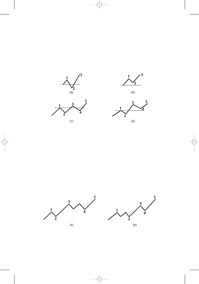
Elliott introduced a series of market patterns that apply to al-

most every situation in market development. If the market rhythm is
regular, wave 2 will not retrace to the beginning of wave 1, and wave
4 will not correct lower than the top of wave 1 (Figure 1.9). In cases
where it still does, the wave count must be adjusted.

Each of the two corrective waves 2 and 4 can be subdivided into

three waves of a smaller degree. Corrective waves 2 and 4 alternate in
pattern. Elliott called this the rule of alternation. If wave 2 is simple,
wave 4 will be complex, and vice versa (Figure 1.10). Complex in this
respect is another term to describe the fact that wave 2 (or wave 4)
consists of subwaves and does not go straight as the simple waves do.

Figure 1.9

Counting is (a) erroneous in a 3-wave upmove; (b) correct in a 3-

wave upmove; (c) erroneous in a 5-wave upmove; (d) correct in a 5-wave up-
move. Source: Fibonacci Applications and Strategies for Traders, by Robert
Fischer (New York: Wiley, 1993), p. 14. Reprinted with permission.

Figure 1.10

Simple waves and complex waves (a) in wave 4; (b) in wave 2.

Source: Fibonacci Applications and Strategies for Traders, by Robert Fischer
(New York: Wiley, 1993), p. 14. Reprinted with permission.

fisc_c01.qxd 8/22/01 8:38 AM Page 17

18

•

BASIC FIBONACCI PRINCIPLES

Given his remarkable observation that simple and complex waves

alternate, and his formulation of this as a rule for market develop-
ment, Elliott linked nature’s law to human behavior and thus to in-
vestors’ behavior.

In natural phenomena such as sunf lowers, pinecones, and pineap-

ples, there are spirals that alternate by f irst turning clockwise and
then counterclockwise. This alternation is seen as an equivalent of the
alternation of simple and complex constellations in the corrective
waves 2 and 4.

In addition to corrections as integral parts of any market move,

Elliott analyzed extensions as reinforcements of trends to either side
of the market, be they uptrends or downtrends. “Extensions may
appear in any one of the three impulse waves, wave 1, 3, or 5, but never
in more than one” (p. 55).

Combinations of impulse waves and extensions in the first, third,

and f ifth wave of a market uptrend are demonstrated in Figure 1.11.
The three wave extensions shown can be reversed for impulse waves
and extensions in downtrends.

At this point, we refrain from giving readers advice on all possi-

ble options given in Elliott’s publications so that we can model the
basic structure of market moves based on impulse waves, corrections,
and extensions.

The purpose of this quick review is to show the essence of El-

liott’s ideas and follow them as they became more intricate. In their

Figure 1.11

(a) First wave extension in an uptrend; (b) third wave extension in

an uptrend; (c) fifth wave extension in an uptrend. Source: Fibonacci Applica-
tions and Strategies for Traders, by Robert Fischer (New York: Wiley, 1993),
p. 17. Reprinted with permission.

fisc_c01.qxd 8/22/01 8:38 AM Page 18

THE ELLIOTT WAVE PRINCIPLE

•

19

most complex stages, it is almost impossible, even for very experienced
Elliott followers, to apply all of Elliott’s wave pattern rules to real-
time trading.

Elliott himself admitted: “Corrections in bull and bear swings

are more difficult to learn” (p. 48). The problem is that the complex na-
ture of the wave structure does not leave room for forecasts of future
price moves in advance. The schemes and structures look perfect in
retrospect. The multitude of rules and situations described by Elliott
can be used to f it any price pattern after the fact. But that is not good
enough for real-time trading.

To conclude our remarks on Elliott, we give a summary of those

segments of Elliott’s f indings that can be exploited in order to devise
trading concepts and trading tools that are easy to apply, and that re-
late to what we have stated about Fibonacci’s PHI as the constant for
natural growth.

Elliott’s principles of markets steadily moving in a wave rhythm

are brilliantly conceived. The principles work perfectly in regular mar-
kets and give stunning results when looking back at the charts.

The most signif icant problem is that market swings are irregu-

lar. This makes it diff icult to give def initive answers to questions
such as:

• Is the point at which we start our wave count part of an impulse

wave or part of a corrective wave?

• Will there be a f ifth wave?

• Is the correction f lat or is it zigzag?

• Will there be an extension in wave 1, 3, or 5?

Elliott specif ically wrote, regarding this point: “The Principle

has been carefully tested and used successfully by subscribers in fore-
casting market movements” (p. 107). And: “Hereafter letters will be
issued on completion of a wave and not await the entire cycle. In this
matter, students may learn how to do their own forecasting and at no
expense. The phenomenon and its practical application become in-
creasingly interesting because the market continually unfolds new ex-
amples to which may be applied unchanging rules” (p. 137).

Our own work with Elliott’s concepts, done from many different

angles over 20 years, does not support the contention that the wave
structure has forecasting ability. The wave structure is too complex,

fisc_c01.qxd 8/22/01 8:38 AM Page 19

20

•

BASIC FIBONACCI PRINCIPLES

especially in the corrective waves. The rule of alternation is extremely
helpful, but this abstract scheme does not tell us, for example, whether
to expect:

• A correction of three waves,

• A double sideways correction, or

• A triple sideways movement.

It is even more unlikely that any 5-wave pattern can be forecast.

The integration of extensions in wave 1, wave 3, or wave 5 complicates
the problem further. The beauty of working with the Elliott concept is
not the wave count. We can only agree when J. R. Hill reveals in his
practical application: “The concept presented is extremely useful but
has literally driven men ‘up the wall’ as they try to f it chart patterns
to exactness in conformity with the Elliott wave” (p. 33).

Elliott focuses on pattern recognition. His whole work is stream-

lined to forecast future price moves based on existing patterns, but he
does not appear to have succeeded in this area.

Elliott expressed uncertainty about the wave count himself,

when he wrote in different newsletters: “The f ive weeks’ sideways
movement was devoid of pattern, a feature never before noted”
(p. 167).

Elsewhere he wrote: “The pattern of the movement across the

bottom is so exceedingly rare that no mention thereof appears in the
Treatises. The details baff le any count” (p. 165).

Yet again: “The time element [meaning the Fibonacci summation

series] as an independent device, however, continues to be baff ling
when attempts are made to apply any known rule of sequence to trend
duration” (p. 180).

And last: “The time element is based on the Fibonacci summation

series but has its limitations and can be used only as an adjunct of the
wave principle” (p. 186).

Elliott did not realize that it is not the wave count that is impor-

tant, but Fibonacci’s PHI. The Fibonacci ratio represents nature’s law
and human behavior. It is no more and no less than Fibonacci’s PHI
that we try to measure in the observation of market swings. While
the Fibonacci summation series and the Fibonacci ratio PHI are con-
stant, the wave count is confusing.

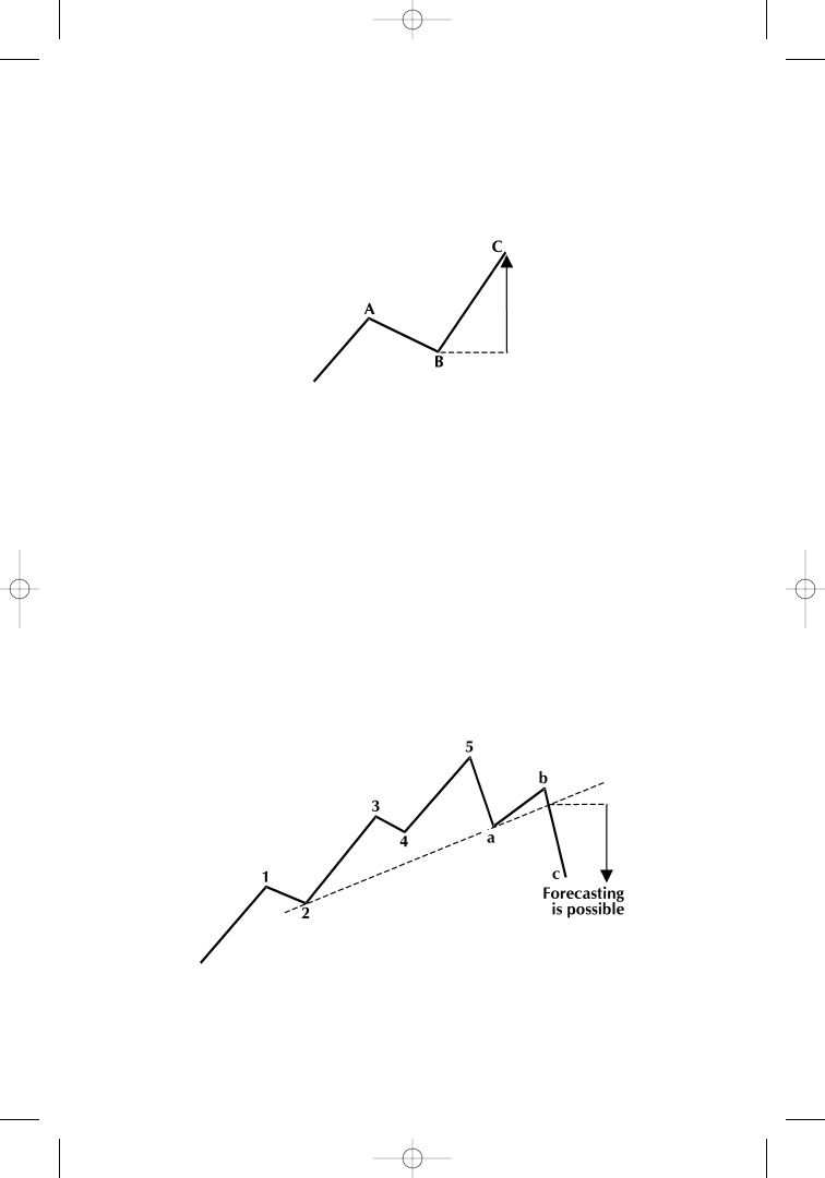
Elliott tried to forecast a price move from point B to point C

based on market patterns (Figure 1.12). We consider this impossible,

fisc_c01.qxd 8/22/01 8:38 AM Page 20

THE ELLIOTT WAVE PRINCIPLE

•

21

and Elliott himself has never given a rule that showed he was able to
do it mechanically.

By studying Elliott’s publications more carefully, a rule with

forecasting value can still be identif ied. “A cyclical pattern or mea-
surement of mass psychology is f ive waves upward and three waves
downward, a total of eight waves. These patterns have forecasting
value: when five waves upward have been completed, three waves down
will follow, and vice versa” (p. 112). We could not agree more with this
statement. Figure 1.13 visualizes Elliott’s latter f indings.

Most likely, Elliott did not realize that his strategy had taken a

complete shift. Elliott’s latest statement takes an opposite strategy,
compared to the approach shown in Figure 1.12. Instead of trying to

Figure 1.12

Forecasting a price move from point B to point C is not possible.

Source: Fibonacci Applications and Strategies for Traders, by Robert Fischer
(New York: Wiley, 1993), p. 23. Reprinted with permission.

Figure 1.13

Forecasting a price move after the end of a 5-wave cycle is possi-

ble. Source: Fibonacci Applications and Strategies for Traders, by Robert Fis-
cher (New York: Wiley, 1993), p. 23. Reprinted with permission.

fisc_c01.qxd 8/22/01 8:38 AM Page 21

22

•

BASIC FIBONACCI PRINCIPLES

forecast a price move from point B to point C, he waits, according to
Figure 1.13, until the very end of the 5-wave move, because three
waves in the opposite direction are to be expected.

We totally accept Elliott’s approach here and will reinforce the

idea with additional rules in later sections. Numbers 5 and 3 are valid
in the Fibonacci summation series and therefore cannot mislead us in
our analysis.

We will also introduce other investment strategies closely related

to the Fibonacci ratio. We will cover corrections and extensions as
Elliott did, but will do so differently, always with our focus on Fi-
bonacci’s ratio PHI and its representation in the instruments we
analyze.

Elliott never worked with a geometric approach. We, however,

have developed computerized PHI-spirals and PHI-ellipses ready for
application to analysis. We strongly believe that this is the solution to
the problem of combining price and time in an integral analysis ap-
proach. This goes far beyond what we initiated with our f irst book
some eight years ago.

Using our Fibonacci trading tools, as well as our WINPHI com-

puter program, our analyses in the forthcoming chapters will concen-
trate mainly on daily price bar charts.

All tools presented have been tested thoroughly and are ready to

be used on the commodity and stock markets. Research shows that in-
traday data can also be used, but under different parameters. More
historical tests are needed on a tick or intraday bar basis before def i-
nite rules can be set for real-time application of Fibonacci-related geo-
metrical tools.

SUMMARY: GEOMETRICAL FIBONACCI TOOLS

Investigation into the Fibonacci summation series and Elliott’s analy-
sis of markets moving in regular waves has led us to six general tools
that can be applied, almost without limit, to market data series,
whether cash currencies, futures, index products, stocks, or mutual
funds are involved.

The six tools are: (1) The Fibonacci summation series itself,

(2) Fibonacci time goals, (3) corrections and extensions in relation
to the Fibonacci ratio, (4) PHI-channels, (5) PHI-spirals, and (6) PHI-
ellipses.

fisc_c01.qxd 8/22/01 8:38 AM Page 22

SUMMARY: GEOMETRICAL FIBONACCI TOOLS

•

23

All six of these trading tools are described in this section, to give

readers an overview of the functioning and the functionality of the
geometrical instruments in any detailed analysis and application of
the tools to market data.

The Fibonacci Summation Series

It might seem astonishing at f irst, but the Fibonacci summation se-
ries can easily be turned into a tool for market analysis that works in
a stable and reliable manner.

We recapitulate the Fibonacci summation series as:

The quotients of each number in the Fibonacci series, divided by the
preceding number, asymptotically gets closer to the value PHI

= 1.618

(which we call the Fibonacci ratio).

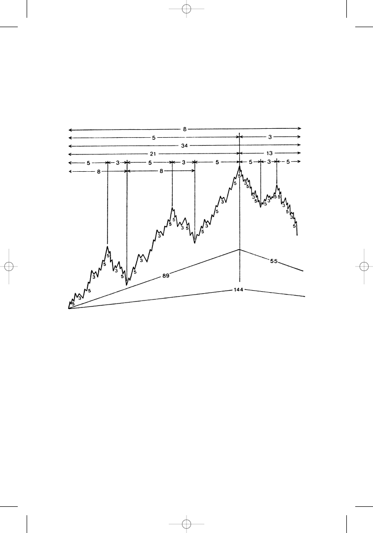
If we combine the f indings of Fibonacci with those of Elliott, we

can count out Elliott’s theoretical waves—five plus three plus five plus
three plus f ive, for a total of 21 major waves, a number of the Fi-
bonacci summation series.

If each 5-wave move in an uptrend is broken down into f ive plus

three plus f ive plus three plus f ive smaller or intermediate waves (a
total of 21 waves), and if each of the resulting waves is broken down
into f ive plus three plus f ive (or a total of 13) small waves, we end up
with a total of 89 waves, a number that we again recognize as part of
the Fibonacci summation series.

If we go through the same process for the three corrective waves,

we come up with a total of 55 waves for the corrective 3-wave move
and a grand total of 144 waves for the completion of one of Elliott’s
market cycles.

The general application of this principle shows that a move in a

particular direction continues up to a point where a time frame—part
of, and consistent with, the f igures of the Fibonacci summation se-
ries—is completed.

A move that extends itself beyond three days should not reverse

until f ive days are reached. A move that exceeds f ive days should last
a minimum of eight days. A trend of nine days should not f inish be-
fore 13 days have passed, and so on.

1 1

2

3

5

8 13 21 34 55 89 144

– –

–

–

–

–

–

–

–

–

–

– . . .

fisc_c01.qxd 8/22/01 8:38 AM Page 23

24

•

BASIC FIBONACCI PRINCIPLES

Our f indings regarding the relation between Fibonacci’s sum-

mation series and Elliott’s wave principle can be summarized as
shown in Figure 1.14.

This basic structure of calculating trend changes may be applied

just as successfully on hourly, daily, weekly, or monthly data. But this
is only an ideal type of pattern, and traders must never expect com-
modities, futures, stock index futures, or stocks to behave in such pre-
cise and predictable manners.

Deviations can and will occur both in time and amplitude, be-

cause individual waves and price patterns are not always likely to de-
velop in a regular way. We also have to keep in mind that the simple
application of the Fibonacci summation series is designed to forecast

Figure 1.14

The Fibonacci summation series schematically integrated into the

complete market cycle according to the Elliott wave count. Source: Fibonacci
Applications and Strategies for Traders, by Robert Fischer (New York: Wiley,
1993), p. 20. Reprinted with permission.

fisc_c01.qxd 8/22/01 8:38 AM Page 24

SUMMARY: GEOMETRICAL FIBONACCI TOOLS

•

25

the length of trend moves, but the number of bars in sideways markets
remains unpredictable.

However, as we will see later on, the f igures 8, 13, 21, 34, and

55 can be of very practical value when applied to work in combina-
tion with other Fibonacci tools. One simple example: While looking
for the length of a standard PHI-ellipse in a product we want to
trade, the easiest way to identify a major trend change is to f irst
check for moves of the length of the Fibonacci f igures 8, 13, 21, 34,
or 55. This does not mean that trend changes will always occur at
the precalculated points after 8, 13, 21, 34, or 55 bars, but it happens
too often to be ignored.

Elliott and his followers tried to calculate major trend changes in

the stock market by applying the f igures from the Fibonacci summa-
tion series to weekly, monthly, and yearly data. This made sense even
though the underlying time frames became very long, and turning
points in historical perspective on a weekly, monthly, or yearly basis
often did not materialize at all. On intraday data, we consider the f ig-
ures of very little value because (1) the markets are extended side-
ways, and (2) the much more erratic market moves during the day,
compared to those from day to day, make the use of Fibonacci f igures
intraday almost impossible for serious analysis. In our analysis, there-
fore, we concentrate on daily data and the figures 8, 13, 21, 34, and 55.

Fibonacci Time-Goal Days

The use of time-goal days as the second of our geometrical Fibonacci
tools is derived from the same rationale as the Fibonacci summa-
tion series.

Time-goal days are those days in the future when a price event

will occur. If we were able to anticipate a day in the future when
prices would reach a prescribed target or reverse direction, it would be
a step forward in market analysis. If we could f ind a way to forecast
the market, we would be able to enter trades or exit positions at the
time of the price change rather than after the fact. In addition, a con-
cept of time-goal days would be dynamic, allowing adjustments to
longer or shorter swings of the market.

Our time analysis is based on the f indings of Euclid of Megara

and his invention of the golden section. This was previously discussed
in the representation of the Fibonacci ratio in geometry and the golden
section of a line.

fisc_c01.qxd 8/22/01 8:38 AM Page 25

26

•

BASIC FIBONACCI PRINCIPLES

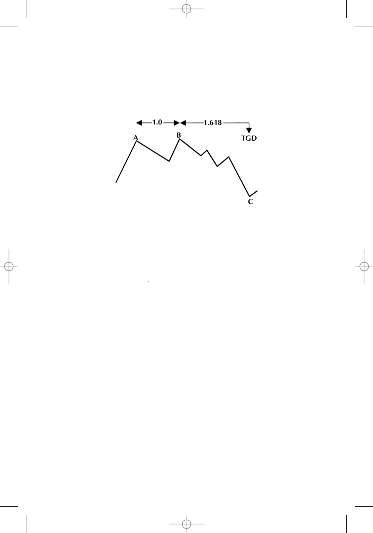
We link nature’s law, expressed in mathematical terms through

the Fibonacci ratio PHI, to market swings, as is illustrated in Fig-
ure 1.15.

When we know the distance from peak A to peak B in days (or

whatever the time unit is), we can multiply this distance by the Fi-
bonacci ratio PHI

= 1.618 to forecast the point C that will occur on

that day:

C is called a Fibonacci time-goal day. This is the day on which

the market is expected to change direction. The forecast of Fibonacci
time-goal days will not indicate whether the price will be high or low
on particular days. The price can be either. In Figure 1.15, we have a
high–high–low formation with a low at point C, but the formation
could also be a high–high–high formation indicating a reversal to the
downside on the precalculated time-goal day. The time-goal day only
forecasts a trend change (a simple event) at the time the goal is
reached; it does not indicate the direction of the event. By applying
the Fibonacci ratio, the timing of objectives can be measured on in-
traday, daily, weekly, or monthly charts.

The Fibonacci summation series, Fibonacci’s PHI, and the no-

tion of time-goal days as the essence of both, are tools that we use to
get closer to resolving the problem of forecasting markets. It cannot be
stressed enough, however, that it is diff icult to wait for a time goal or
to wait for a precalculated period of time (according to the Fibonacci

C

B

B

A

= +

×

−

(

)

1 618

.

Figure 1.15

Calculation of time-goal days. Source: FAM Research, 2000.

fisc_c01.qxd 8/22/01 8:38 AM Page 26

SUMMARY: GEOMETRICAL FIBONACCI TOOLS

•

27

summation series) before finally being entitled to show trading action.
Identifying a Fibonacci goal and patiently sticking to it, even when
the odds are unfavorable (that is, if the market starts moving before
the Fibonacci goal has been reached and one is not yet participating
in the trend), are two sides of the same (golden) trading model.

Corrections and Extensions

Corrections and extensions are the third category of our geometrical
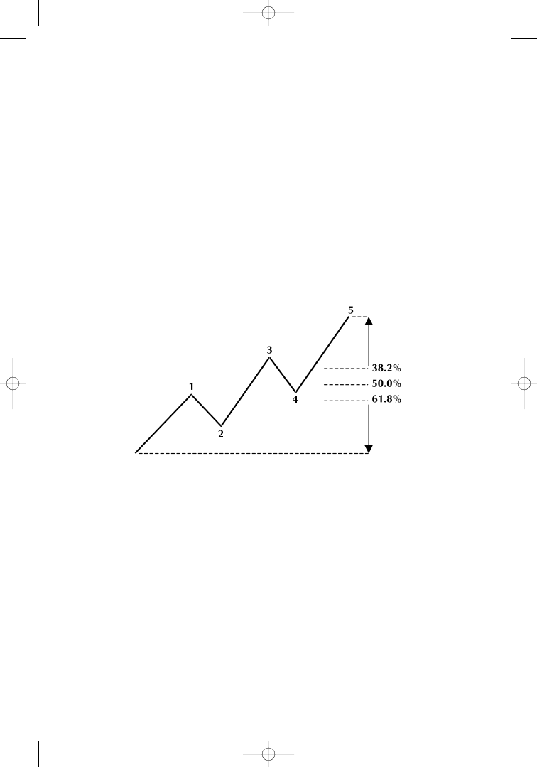
Fibonacci trading tools. The most common approach to working with
corrections is to relate the size of a correction to a percentage of a
prior impulsive market move (Figure 1.16).

In our analysis, we are interested in the three most prominent

percentage values of possible market corrections that can be directly
derived from the quotients of the PHI series and the Fibonacci
sequence:

• 38.2% is the result of 0.618 ÷ 1.618;

• 50.0% is the transformed ratio 1.000; and

• 61.8% is the result of the immediate ratio 1.000 ÷ 1.618.

Figure 1.16

Corrections of 38.2%, 50.0%, and 61.8% after a 5-wave move.

Source: Fibonacci Applications and Strategies for Traders, by Robert Fischer
(New York: Wiley, 1993), p. 52. Reprinted with permission.

fisc_c01.qxd 8/22/01 8:38 AM Page 27

28

•

BASIC FIBONACCI PRINCIPLES

Forecasting the exact size of a correction is an empirical prob-

lem; investing after a correction of just 38.2% might be too early,
whereas waiting for a correction of 61.8% might result in missing
strong trends completely. However, no matter what sizes of corrections
are taken into consideration, the PHI-related sizes are the ones to
focus on in the f irst place.

Extensions, in contrast to corrections, are exuberant price move-

ments. They express themselves in runaway markets, opening gaps,
limit up and limit down moves, and high volatility. These situations
may offer extraordinary trading potential as long as the analysis is
carried out in accordance with sensible and def inite rules.

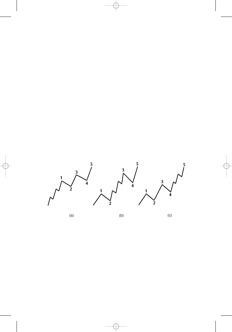
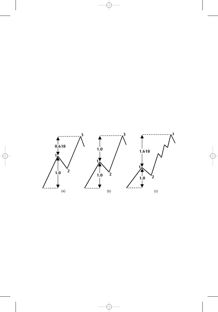
Considering extensions as graphical tools for market analysis,

we again make use of the Fibonacci ratio as we derived it from the
Fibonacci summation series (Figure 1.17).

The three ratios we work with in most of our analyses of exten-

sion sizes are 0.618, 1.000, and 1.618. But other elements of the PHI
series, such as 2.618, 4.236, or 6.854, referred to in earlier sections,
are also valid estimates for the strength of a market move once the
size of the initial wave has been set to 1.000.

Strong trends can overshoot the initial wave by more than just

PHI or 1.618 times the size of the initiating impulse wave. It can be

Figure 1.17

Extensions in the third wave of a trend, and the Fibonacci ratio

PHI. (a) Ratio 0.618; (b) ratio 1.000; (c) ratio 1.618. Source: Fibonacci Appli-
cations and Strategies for Traders, by Robert Fischer (New York: Wiley, 1993),
p. 52. Reprinted with permission.

fisc_c01.qxd 8/22/01 8:38 AM Page 28

SUMMARY: GEOMETRICAL FIBONACCI TOOLS

•

29

tested empirically on various sets of data (using the ratio that best
serves the need of the analyst) to get the most prof it out of mar-
ket rallies.

Remember: If 1.618 does not seem good enough, wait until the

move has extended to 2.618, and do not stop somewhere in the middle.

There is no rationale behind the Fibonacci ratio, but by applying

this ratio as a scheme for analysis, we get a hold on strong major mar-
ket moves that are triggered by news of political or economic events,
crop or storage reports, or any situation in which emotions take con-
trol of actions. Fear or greed, fast markets or stop-loss orders make the
markets move. We measure the extent of these moves in Fibonacci’s
ratio PHI, the Fibonacci summation series, and the member numbers
of the respective PHI series.

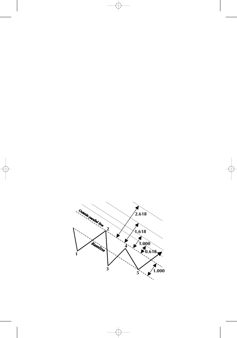
PHI-Channels

PHI-channels, so-called Fibonacci trend channels, constitute the
fourth element in our set of geometrical tools. They are generated by
drawing parallel lines through tops and bottoms of price moves.

The general idea behind PHI-channels as Fibonacci-related trad-

ing tools becomes clear when we look at the abstract schematic pre-
sentation in Figure 1.18.

Figure 1.18

PHI-channel. Source: FAM Research, 2000.

fisc_c01.qxd 8/22/01 8:38 AM Page 29

30

•

BASIC FIBONACCI PRINCIPLES

The width of the PHI-channel is calculated as the distance be-

tween the baseline and the parallel outside line. This distance is set
to 1.000. Parallel lines are then drawn in PHI series distance starting
at 0.618 times the size of the channel, continuing at 1.000 times, 1.618
times, 2.618 times, 4.236 times the distance, and so on. We follow the
wave pattern move through the PHI-channel. As soon as wave 5 has
been completed, we expect a correction opposite to the trend direction
to occur.

In contrast to our f indings regarding corrections aiming at the

prediction of price targets, PHI-channels provide us with an extra op-
portunity to make assumptions about the duration of the expected
correction timewise. The correction will last until either one of the
lines running parallel to the trend channel is touched. Which line we
should wait for is another empirical question, but regardless of which
line we consider reliable (0.618, 1.000, 1.618, 2.618, or beyond), we
must make sure that we wait to the very end and do not act before the
Fibonacci target line has been reached.

At the point our target parallel is realized, we might not have ar-

rived at our Fibonacci goal pricewise on the basis of our calculation of
corrections. This example shows how important it is to work with mul-
tiple Fibonacci targets and to try to identify points where different
Fibonacci tools result in the same forecast pricewise and /or timewise.

In our example, an optimal Fibonacci target would be triggered

when a correction out of a Fibonacci trend channel hit a parallel at
0.618, 1.000, 1.618, or 2.618 times the size of the channel, and price-
wise at a level where a correction of 38.2%, 50.0%, or 61.8% is just or
nearly completed.

In discussions of similar examples in later sections,we prove how

this kind of multiple Fibonacci analysis is possible.

PHI-Spirals

PHI-spirals, f ifth on our list of Fibonacci tools, provide the optimal
link between price and time analysis.

In an earlier section on the representation of Fibonacci’s PHI in

geometry, we introduced the PHI-spirals as perfect geometric approx-
imations of nature’s law and phenomena of natural growth in the
world around us.

In simple geometrical terms, the size of a PHI-spiral is deter-

mined by the distance between the center (X) of the spiral and the
starting point (A). The starting point is usually given by wave 1 or

fisc_c01.qxd 8/22/01 8:38 AM Page 30

SUMMARY: GEOMETRICAL FIBONACCI TOOLS

•

31

wave 2: either a peak in uptrends or a valley in downtrends. The cor-
responding center of the spiral is usually set to the beginning of the
respective wave. The PHI-spiral then turns either clockwise or coun-
terclockwise around the initial line that goes from the center to the
starting point.

As the PHI-spiral grows, it extends by a constant ratio with every

full cycle. Returning to what we explained earlier in this chapter, all
the spirals that have rates of growth corresponding to an element of
the PHI series— 0.618, 1.000, 1.618, 2.618, and so on—shall, in the
context of this book, be referred to as PHI-spirals (Figure 1.19).

A growth rate of 1.618 is the one we will work with most, but

all other ratios that can be generated using the PHI series are valid
as well and can be tested individually with the WINPHI software
package.

Figure 1.19

PHI-spiral. Source: FAM Research, 2000.

fisc_c01.qxd 8/22/01 8:38 AM Page 31

32

•

BASIC FIBONACCI PRINCIPLES

We can now conclude that each point on a PHI-spiral manifests

an optimal combination of price and time. Corrections and trend
changes occur at all those prominent points where the PHI-spiral is
touched on its growth path through price and time.

With PHI-spirals as Fibonacci tools, we can make the best out of

the stunning symmetry in the price patterns of charts, whether on a
daily, weekly, monthly, or yearly basis, and whether they represent
stocks, cash currencies, commodities, or derivatives. The stronger the
behavioral patterns become in extreme market conditions, the better
PHI-spirals work to inform investors in advance about tops and bot-
toms of market moves.

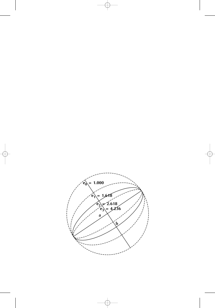
PHI-Ellipses

The sixth tool brings us back to the PHI-ellipse. In its geometry, it is
like the PHI-spiral. This tool has been discussed in one of the earlier
sections.

An ellipse is the mathematical expression of an oval. What we

mainly are interested in when dealing with a Fibonacci tool is the ratio
e

x

= a ÷ b of major axis a and minor axis b of the ellipse (Figure 1.20).

An ellipse is turned into a PHI-ellipse in all those cases where

the ratio of the major axis, divided by the minor axis of the ellipse, is

Figure 1.20

PHI-ellipses; e

x

= a ÷ b. Source: FAM Research, 2000.

fisc_c01.qxd 8/22/01 8:38 AM Page 32

SUMMARY: GEOMETRICAL FIBONACCI TOOLS

•

33

a member number of the PHI series— 0.618–1.000–1.618–2.618, and
so on. A circle, in this respect, is a special type of PHI-ellipse with
a

= b (ratio a ÷ b = 1).

What makes PHI-ellipses preferable to all other possible ellipses

with ratios of major axis divided by minor axis other than numbers of
the PHI series is that empirical research has shown that the majority
of people f ind approximations of PHI-ellipses signif icantly more vi-
sually satisfying. But when it comes to using PHI-ellipses as tools for
market analysis, satisfaction is not what we f irst consider. We are pri-
marily looking for ellipses that f it well to market moves and can be
utilized for forecasting purposes.

From Figure 1.20, we can conclude that PHI-ellipses with in-

creasing ratios e

x

= a ÷ b of major axis to minor axis turn very quickly

into “Havana cigars”—and, in this process, lose part of their beauty.
PHI-ellipses at ratios of 6.854 and above become so narrow that they
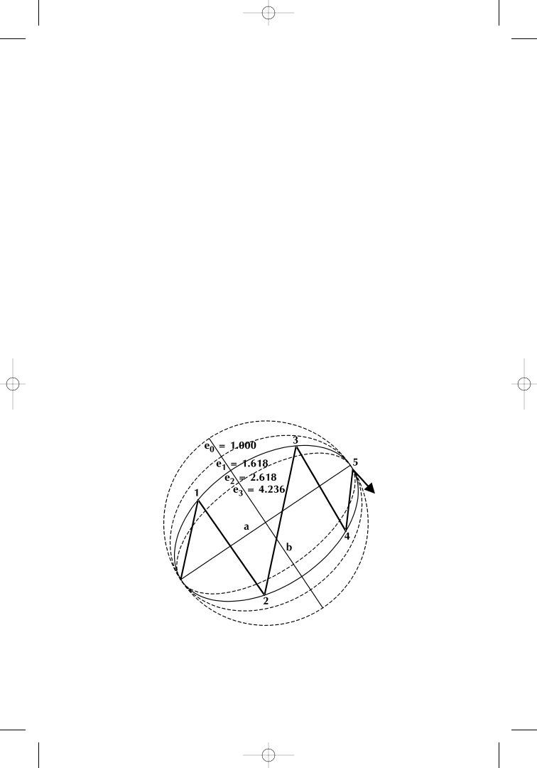
can hardly be applied to charts as analytical tools. In Figure 1.21,
however, we present a convincing solution that helps us with the
dilemma and gives us a chance to maintain the beauty of PHI-ellipses
up to ratios of at least 17.944.

To make PHI-ellipses work as tools for chart analysis, we have

applied a transformation to the underlying mathematical formula that

Figure 1.21

Fischer transformed PHI-ellipses; e

x

= (a ÷ b)*. Source: FAM Re-

search, 2000.

fisc_c01.qxd 8/22/01 8:38 AM Page 33

34

•

BASIC FIBONACCI PRINCIPLES

describes the shape of the ellipse. We still consider the ratio of major
axis a to minor axis b of the ellipse, but in a different way—in math-
ematical terms e

x

= (a ÷ b)*.

It took us quite a while to come up with a solution to the problem

of transforming PHI-ellipses for productive chart analysis and, at the
same time, maintaining them as PHI-ellipses; that is, still incorpo-
rating the member numbers of the PHI series into our analysis of the
ratio of the major axes and minor axes of the ellipse.

We protect our property in this case and hold the exact formula

for transforming a ÷ b into (a ÷ b)* proprietary, but readers will still
benef it from our f indings, because transformed PHI-ellipses are part
of the WINPHI software on the CD-ROM and can easily be applied to
charts, according to readers’ preferences.

However, when we refer to the application of PHI-ellipses, keep

in mind that we are referring to Fischer-transformed PHI-ellipses of
the type demonstrated in Figure 1.21.

As long as we prefer a PHI-ellipse [meaning an ellipse with a

ratio of major axis to minor axis (a ÷ b)*, which is an element of the
PHI series], we are free to test various ratios and ellipses on market
data. The only thing we must make sure of is that once we have found
an ellipse that f its well to a move (like the one at a ratio of (a ÷ b)*

=

2.618 in Figure 1.21), we do not alter it in the course of our analysis.

We will see in the upcoming chapters how this promising tool can

be applied to charts and can be used to forecast market moves and
targets in market developments.

Final Introductory Remarks on the WINPHI Software Package

The WINPHI software package that comes with this book allows in-
terested investors to generate all the signals on historical data with
the different Fibonacci tools (shown in examples).

All sample signals were tested, via our best efforts, by the time

this book was completed early in 2001. Tests were done by hand and,
of course, with the assistance of the WINPHI computer program.

Generating signals by hand can introduce the possibility of

error. More important to mention, we did not test the products for
demonstration purposes longer than 11 months backward on daily
charts and three years backward on weekly charts. It would be too
much for us to test each strategy presented in our entire historical
database, which goes between 12 and 20 years backward, depending

fisc_c01.qxd 8/22/01 8:38 AM Page 34

SUMMARY: GEOMETRICAL FIBONACCI TOOLS

•

35

on the product. However, interested investors have the ability to do
this on sample datasets for all major products and markets included
with the CD-ROM, or on their own datasets.

We do not claim that, for each example shown, we have published

the very best parameters, entry rules, stop-loss rules, or profit targets.
There will certainly be other combinations that are somewhat supe-
rior to what we offer, but we want to distribute inspiration rather than
optimization. We therefore provide a challenge for every investor who
is especially interested in one of the tools or in a special strategy.

Test runs become more valid and reliable, the longer the time

span selected to test a tool or a strategy. This holds true for all the ex-
amples and strategies we have described. Parameters, like swing
sizes, never work equally well in sideways market conditions and in
trending markets. This factor becomes especially important when we
work with extensions or corrections where percentages are calculated
relative to a minimum swing size. It is possible that the relevant pa-
rameters we use change over time with longer historical test runs.

In addition, the WINPHI software is basically restricted to plot-

ting daily data on charts in ASCII D–O–H–L–C f ield order. We do not
offer any conversion utility; the program does not change compression
rates from daily to weekly, monthly, or yearly. However, weekly,
monthly, yearly, and even intraday minute or hourly bar charts can be
generated, if the data to plot are already in the respective ASCII
D–O–H–L–C format. Monthly ASCII data f iles are plotted as monthly
data, weekly data f iles as weekly data, and so on. And if data come as
intraday minute or hourly ASCII D–O–H–L–C data, the correct data
compression will also be plotted on the charts. Nevertheless, our de-
fault assumption remains that daily ASCII-coded D–O–H–L–C data
f iles are intended to be analyzed by users.

All six Fibonacci tools are based on pattern recognition. These

patterns can look very different if the price scale is varied. Generally
speaking, online data vendors provide software packages that, by de-
fault, always scale full screen when information is updated. Depend-
ing on new highs or new lows, price scales are adjusted accordingly.

However, a constant scale is an absolutely necessary condition

for any sort of convincing pattern recognition that is intended to run
over longer periods of time (sometimes 20 years or more). One year of
data, scaled full screen, is usually not good enough to cover an entire
market cycle of trending and sideways periods. As soon as sophisti-
cated tools, such as the PHI-ellipse, are employed to analyze market

fisc_c01.qxd 8/22/01 8:38 AM Page 35

36

•

BASIC FIBONACCI PRINCIPLES

moves in price and in time, it is vital to have the angle of the PHI-
ellipse remain free of inf luence from small variations in scaling.

Knowing that many data vendors do not have a feature for con-

stant scaling included with their charting devices, we designed our
software so that users can opt for either full-screen scaling of the most
recent data loaded or constant scaling from highest high to lowest low
of the entire data series for investors who do not feel comfortable with
the need to convert data from their data series.

FINAL REMARKS

Elliott and his followers did not f ind a solution to the problem of
whether to chart data on a linear scale or on a semi-log scale. Semi-log
scales might be interesting to look at, especially when weekly or
monthly charts analyze price and time, or when working with correc-
tions or extensions. We consider the discussion on linear or semi-log
scaling important to professional traders. Throughout the book, all
sample applications of our tools have been conducted using linear scal-
ing. Wherever we f ind it necessary—for example, when describing ex-
tensions and corrections on weekly data—we discuss the subject
brief ly. However, we do not consider the matter worth the effort of
integrating an extra feature for semi-log scaling with our WINPHI
software package.

So much for technical questions, parameters, scaling, and mea-

surement. May the following chapters be inspiring and challenging.
Readers should take our f indings not as f inal solutions to the problem
of making Fibonacci’s PHI tradable, but as a promising starting point
to verify, modify, improve, and apply our Fibonacci tools.

Trading according to Fibonacci principles is a journey. Come join

us for an exciting trip.

fisc_c01.qxd 8/22/01 8:38 AM Page 36