19

Jacobian Linearizations, equilibrium points

In modeling systems, we see that nearly all systems are nonlinear, in that the dif-
ferential equations governing the evolution of the system’s variables are nonlinear.
However, most of the theory we have developed has centered on linear systems.
So, a question arises: “In what limited sense can a nonlinear system be viewed as
a linear system?” In this section we develop what is called a “Jacobian lineariza-
tion of a nonlinear system,” about a specific operating point, called an equilibrium
point.

19.1

Equilibrium Points

Consider a nonlinear differential equation

˙x(t) = f (x(t), u(t))

(72)

where f is a function mapping R

n

× R

m

→ R

n

. A point ¯

x ∈ R

n

is called an

equilibrium point if there is a specific ¯

u ∈ R

m

(called the equilibrium input)

such that

f (¯

x, ¯

u) = 0

n

Suppose ¯

x is an equilibrium point (with equilibrium input ¯

u). Consider starting

the system (72) from initial condition x(t

0

) = ¯

x, and applying the input u(t) ≡ ¯u

for all t ≥ t

0

. The resulting solution x(t) satisfies

x(t) = ¯

x

for all t ≥ t

0

. That is why it is called an equilibrium point.

19.2

Deviation Variables

Suppose (¯

x, ¯

u) is an equilibrium point and input. We know that if we start the

system at x(t

0

) = ¯

x, and apply the constant input u(t) ≡ ¯u, then the state of the

system will remain fixed at x(t) = ¯

x for all t. What happens if we start a little

bit away from ¯

x, and we apply a slightly different input from ¯

u? Define deviation

variables to measure the difference.

δ

x

(t) := x(t) − ¯x

δ

u

(t) := u(t) − ¯u

In this way, we are simply relabling where we call 0. Now, the variables x(t) and
u(t) are related by the differential equation

˙x(t) = f (x(t), u(t))

169

From _Dynamic Systems and Feedback_
by Packard, Poola, Horowitz, 2002

Copyright 2002, Andrew Packard
All rights reserved.
Do not duplicate or redistribute.

Substituting in, using the constant and deviation variables, we get

˙δ

x

(t) = f (¯

x + δ

x

(t), ¯

u + δ

u

(t))

This is exact. Now however, let’s do a Taylor expansion of the right hand side,
and neglect all higher (higher than 1st) order terms

˙δ

x

(t) ≈ f (¯x, ¯u) +

∂f
∂x

¯

¯

¯

¯

¯

x=¯

x

u=¯

u

δ

x

(t)

+

∂f
∂u

¯

¯

¯

¯

¯

x=¯

x

u=¯

u

δ

u

(t)

But f (¯

x, ¯

u) = 0, leaving

˙δ

x

(t) ≈

∂f
∂x

¯

¯

¯

¯

¯

x=¯

x

u=¯

u

δ

x

(t)

+

∂f
∂u

¯

¯

¯

¯

¯

x=¯

x

u=¯

u

δ

u

(t)

This differential equation approximately governs (we are neglecting 2nd order and
higher terms) the deviation variables δ

x

(t) and δ

u

(t), as long as they remain

small. It is a linear, time-invariant, differential equation, since the derivatives of
δ

x

are linear combinations of the δ

x

variables and the deviation inputs, δ

u

. The

matrices

A :=

∂f
∂x

¯

¯

¯

¯

¯

x=¯

x

u=¯

u

∈ R

n×n

,

B :=

∂f
∂u

¯

¯

¯

¯

¯

x=¯

x

u=¯

u

∈ R

n×m

(73)

are constant matrices. With the matrices A and B as defined in (73), the linear
system

˙δ

x

(t) = Aδ

x

(t)

+

Bδ

u

(t)

is called the Jacobian Linearization of the original nonlinear system (72), about
the equilibrium point (¯

x, ¯

u). For “small” values of δ

x

and δ

u

, the linear equation

approximately governs the exact relationship between the deviation variables δ

u

and δ

x

.

For “small” δ

u

(ie., while u(t) remains close to ¯

u), and while δ

x

remains “small”

(ie., while x(t) remains close to ¯

x), the variables δ

x

and δ

u

are related by the

differential equation

˙δ

x

(t) = Aδ

x

(t)

+

Bδ

u

(t)

In some of the rigid body problems we considered earlier, we treated problems
by making a small-angle approximation, taking θ and its derivatives ˙θ and ¨

θ very

small, so that certain terms were ignored ( ˙θ

2

, ¨

θ sin θ) and other terms simplified

(sin θ ≈ θ, cos θ ≈ 1). In the context of this discussion, the linear models we
obtained were, in fact, the Jacobian linearizations around the equilibrium point
θ = 0, ˙θ = 0.

If we design a controller that effectively controls the deviations δ

x

, then we have

designed a controller that works well when the system is operating near the equi-
librium point (¯

x, ¯

u). We will cover this idea in greater detail later. This is a

common, and somewhat effective way to deal with nonlinear systems in a linear
manner.

170

19.3

Tank Example

Consider a mixing tank, with constant supply temperatures T

C

and T

H

. Let the

inputs be the two flow rates q

C

(t) and q

H

(t). The equations for the tank are

˙h(t) =

1

A

T

³

q

C

(t) + q

H

(t) − c

D

A

o

q

2gh(t)

´

˙

T

T

(t) =

1

h(t)A

T

(q

C

(t) [T

C

− T

T

(t)] + q

H

(t) [T

H

− T

T

(t)])

Let the state vector x and input vector u be defined as

x(t) :=

"

h(t)

T

T

(t)

#

,

u(t) :=

"

q

C

(t)

q

H

(t)

#

f

1

(x, u) =

1

A

T

³

u

1

+ u

2

− c

D

A

o

√

2gx

1

´

f

2

(x, u) =

1

x

1

A

T

(u

1

[T

C

− x

2

] + u

2

[T

H

− x

2

])

Intuitively, any height ¯h > 0 and any tank temperature ¯

T

T

satisfying

T

C

≤ ¯

T

T

≤ T

H

should be a possible equilibrium point (after specifying the correct values of the
equilibrium inputs). In fact, with ¯h and ¯

T

T

chosen, the equation f (¯

x, ¯

u) = 0 can

be written as

"

1

1

T

C

− ¯x

2

T

H

− ¯x

2

# "

¯

u

1

¯

u

2

#

=

"

c

D

A

o

√

2g¯

x

1

0

#

The 2 × 2 matrix is invertible if and only if T

C

6= T

H

. Hence, as long as T

C

6= T

H

,

there is a unique equilibrium input for any choice of ¯

x. It is given by

"

¯

u

1

¯

u

2

#

=

1

T

H

− T

C

"

T

H

− ¯x

2

−1

¯

x

2

− T

C

1

# "

c

D

A

o

√

2g¯

x

1

0

#

This is simply

¯

u

1

=

c

D

A

o

√

2g¯

x

1

(T

H

− ¯x

2

)

T

H

− T

C

,

¯

u

2

=

c

D

A

o

√

2g¯

x

1

(¯

x

2

− T

C

)

T

H

− T

C

Since the u

i

represent flow rates into the tank, physical considerations restrict

them to be nonegative real numbers. This implies that ¯

x

1

≥ 0 and T

C

≤ ¯

T

T

≤ T

H

.

Looking at the differential equation for T

T

, we see that its rate of change is inversely

related to h. Hence, the differential equation model is valid while h(t) > 0, so
we further restrict ¯

x

1

> 0. Under those restrictions, the state ¯

x is indeed an

equilibrium point, and there is a unique equilibrium input given by the equations
above.

Next we compute the necessary partial derivatives.

"

∂f

1

∂x

1

∂f

1

∂x

2

∂f

2

∂x

1

∂f

2

∂x

2

#

=





−

gc

D

A

o

A

T

√

2gx

1

0

−

u

1

[T

C

−x

2

]+u

2

[T

H

−x

2

]

x

2

1

A

T

−(u

1

+u

2

)

x

1

A

T





171

"

∂f

1

∂u

1

∂f

1

∂u

2

∂f

2

∂u

1

∂f

2

∂u

2

#

=

"

1

A

T

1

A

T

T

C

−x

2

x

1

A

T

T

H

−x

2

x

1

A

T

#

The linearization requires that the matrices of partial derivatives be evaluated at
the equilibrium points. Let’s pick some realistic numbers, and see how things
vary with different equilibrium points. Suppose that T

C

= 10

◦

, T

H

= 90

◦

, A

T

=

3m

2

, A

o

= 0.05m, c

D

= 0.7. Try ¯h = 1m and ¯h = 3m, and for ¯

T

T

, try ¯

T

T

= 25

◦

and

¯

T

T

= 75

◦

. That gives 4 combinations. Plugging into the formulae give the 4 cases

1.

³

¯h, ¯

T

T

´

= (1m, 25

◦

). The equilibrium inputs are

¯

u

1

= ¯

q

C

= 0.126

,

¯

u

2

= ¯

q

H

= 0.029

The linearized matrices are

A =

"

−0.0258

0

0

−0.517

#

,

B =

"

0.333 0.333

−5.00 21.67

#

2.

³

¯h, ¯

T

T

´

= (1m, 75

◦

). The equilibrium inputs are

¯

u

1

= ¯

q

C

= 0.029

,

¯

u

2

= ¯

q

H

= 0.126

The linearized matrices are

A =

"

−0.0258

0

0

−0.0517

#

,

B =

"

0.333

0.333

−21.67 5.00

#

3.

³

¯h, ¯

T

T

´

= (3m, 25

◦

). The equilibrium inputs are

¯

u

1

= ¯

q

C

= 0.218

,

¯

u

2

= ¯

q

H

= 0.0503

The linearized matrices are

A =

"

−0.0149

0

0

−0.0298

#

,

B =

"

0.333

0.333

−1.667 7.22

#

4.

³

¯h, ¯

T

T

´

= (3m, 75

◦

). The equilibrium inputs are

¯

u

1

= ¯

q

C

= 0.0503

,

¯

u

2

= ¯

q

H

= 0.2181

The linearized matrices are

A =

"

−0.0149

0

0

−0.0298

#

,

B =

"

0.333 0.333

−7.22 1.667

#

172

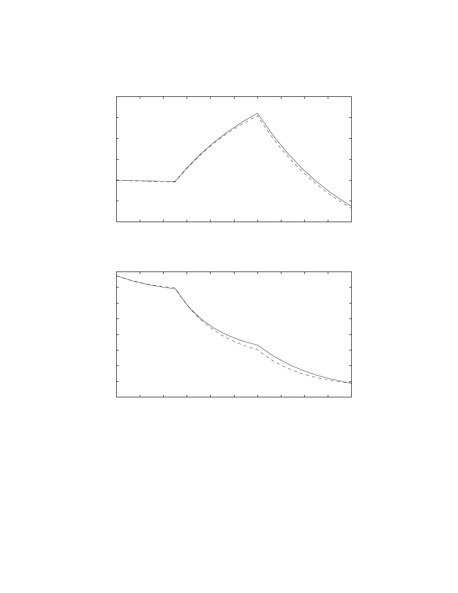
We can try a simple simulation, both in the exact nonlinear equation, and the
linearization, and compare answers.

We will simulate the system

˙x(t) = f (x(t), u(t))

subject to the following conditions

x(0) =

"

1.10
81.5

#

and

u

1

(t) =

(

0.022 for 0 ≤ t ≤ 25
0.043 for 25 < t ≤ 100

u

2

(t) =

(

0.14

for 0 ≤ t ≤ 60

0.105 for 60 < t ≤ 100

This is close to equilibrium condition #2. So, in the linearization, we will use
linearization #2, and the following conditions

δ

x

(0) = x(0) −

"

1

75

#

=

"

0.10

6.5

#

and

δ

u

1

(t) := u

1

(t) − ¯u

1

=

(

−0.007 for 0 ≤ t ≤ 25
0.014

for 25 < t ≤ 100

δ

u

2

(t) := u

2

(t) − ¯u

2

=

(

0.014

for 0 ≤ t ≤ 60

−0.021 for 60 < t ≤ 100

To compare the simulations, we must first plot x(t) from the nonlinear simulation.
This is the “true” answer. For the linearization, we know that δ

x

approximately

governs the deviations from ¯

x. Hence, for that simulation we should plot ¯

x + δ

x

(t).

These are shown below for both h and T

T

.

173

0

10

20

30

40

50

60

70

80

90

100

1

1.05

1.1

1.15

1.2

1.25

1.3

Water Height: Actual (solid) and Linearization (dashed)

Meters

0

10

20

30

40

50

60

70

80

90

100

66

68

70

72

74

76

78

80

82

Water Temp: Actual (solid) and Linearization (dashed)

Degrees

Time

19.4

Linearizing about general solution

In section 19.2, we discussed the linear differential equation which governs small
deviations away from an equilibrium point. This resulted in a linear, time-invariant
differential equation.

Often times, more complicated situations arise. Consider the task of controlling a
rocket trajectory from Earth to the moon. By writing out the equations of motion,
from Physics, we obtain state equations of the form

˙x(t) = f (x(t), u(t), d(t), t)

(74)

where u is the control input (thrusts), d are external disturbances.

174

Through much computer simulation, a preplanned input schedule is developed,
which, under ideal circumstances (ie., d(t) ≡ 0), would get the rocket from Earth
to the moon. Denote this preplanned input by ¯

u(t), and the ideal disturbance by

¯

d(t) (which we assume is 0). This results in an ideal trajectory ¯

x(t), which solves

the differential equation,

˙¯x(t) = f

³

¯

x(t), ¯

u(t), ¯

d(t), t

´

Now, small nonzero disturbances are expected, which lead to small deviations in
x, which must be corrected by small variations in the pre-planned input u. Hence,
engineers need to have a model for how a slightly different input ¯

u(t) + δ

u

(t) and

slightly different disturbance ¯

d(t) + δ

d

(t) will cause a different trajectory. Write

x(t) in terms of a deviation from ¯

x(t), defining δ

x

(t) := x(t) − ¯x(t), giving

x(t) = ¯

x(t) + δ

x

(t)

Now x, u and d must satisfy the differential equation, which gives

˙x(t) = f (x(t), u(t), d(t), t)

˙¯x(t) + ˙δ

x

(t) = f

³

¯

x(t) + δ

x

(t), ¯

u(t) + δ

u

(t), ¯

d(t) + δ

d

(t), t

´

≈ f (¯x(t), ¯u(t), 0, t) +

∂f
∂x

¯

¯

¯

x(t)=¯

x(t)

u(t)=¯

u(t)

d(t)= ¯

d(t)

δ

x

(t) +

∂f
∂u

¯

¯

¯

x(t)=¯

x(t)

u(t)=¯

u(t)

d(t)= ¯

d(t)

δ

u

(t) +

∂f

∂d

¯

¯

¯

x(t)=¯

x(t)

u(t)=¯

u(t)

d(t)= ¯

d(t)

δ

d

(t)

But the functions ¯

x and ¯

u satisfy the governing differential equation, so ˙¯

x(t) =

f (¯

x(t), ¯

u(t), 0, t), leaving the (approximate) governing equation for δ

x

˙¯x(t) =

∂f
∂x

¯

¯

¯

¯

¯

x(t)=¯

x(t)

u(t)=¯

u(t)

d(t)= ¯

d(t)

δ

x

(t) +

∂f
∂u

¯

¯

¯

¯

¯

x(t)=¯

x(t)

u(t)=¯

u(t)

d(t)= ¯

d(t)

δ

u

(t) +

∂f

∂d

¯

¯

¯

¯

¯

x(t)=¯

x(t)

u(t)=¯

u(t)

d(t)= ¯

d(t)

δ

d

(t)

Define time-varying matrices A, B

1

and B

2

by

A(t) :=

∂f
∂x

¯

¯

¯

¯

¯

x(t)=¯

x(t)

u(t)=¯

u(t)

d(t)= ¯

d(t)

B

1

(t) :=

∂f
∂u

¯

¯

¯

¯

¯

x(t)=¯

x(t)

u(t)=¯

u(t)

d(t)= ¯

d(t)

B

2

(t) :=

∂f

∂d

¯

¯

¯

¯

¯

x(t)=¯

x(t)

u(t)=¯

u(t)

d(t)= ¯

d(t)

The deviation variables are approximately governed by

˙δ

x

(t) = A(t)δ

x

(t) + B

1

(t)δ

u

(t) + B

2

(t)δ

d

(t) = A(t)δ

x

(t) +

h

B

1

(t) B

2

(t)

i

"

δ

u

(t)

δ

d

(t)

#

This is called the linearization of system (74) about the trajectory

³

¯

x, ¯

u, ¯

d

´

. This

type of linearization is a generalization of linearizations about equilibrium points.
Linearizing about an equilibrium point yields a LTI system, while linearizing about
a trajectory yields an LTV system.

In general, these types of calculations are carried out numerically,

• simulink to get solution ¯x(t) given particular inputs ¯u(t) and ¯

d(t)

175

• Numerical evaluation of

∂f
∂x

, etc, evaluated at the solution points

• Storing the time-varying matrices A(t), B

1

(t), B

2

(t) for later use

In a simple case it is possible to analytically determine the time-varying matrices.

19.5

Problems

1. The temperature in a particular 3-dimensional solid is a function of position,

and is known to be

T (x, y, z) = 42 + (x − 2)

2

+ 3 (y − 4)

2

− 5 (z − 6)

2

+ 2yz

(a) Find the first order approximation (linearization) of the temperature

near the location (4, 6, 0). Use δ

x

, δ

y

and δ

z

as your deviation variables.

(b) What is the maximum error between the actual temperature and the

first order approximation formula for |δ

x

| ≤ 0.3, |δ

y

| ≤ 0.2, |δ

z

| ≤ 0.1.

You may use Matlab to solve this numerically, or analytically if you
wish.

(c) More generally, suppose that ¯

x ∈ R, ¯y ∈ R, ¯z ∈ R. Find the first order

approximation of the temperature near the location (¯

x, ¯

y, ¯

z).

2. The pitching-axis of a tail-fin controlled missile is governed by the nonlinear

state equations

˙α(t) = K

1

M f

n

(α(t), M ) cos α(t) + q(t)

˙q(t) = K

2

M

2

[f

m

(α(t), M ) + Eu(t)]

Here, the states are x

1

:= α, the angle-of-attack, and x

2

:= q, the angular

velocity of the pitching axis. The input variable, u, is the deflection of the
fin which is mounted at the tail of the missile. K

1

, K

2

, and E are physical

constants, with E > 0. M is the speed (Mach) of the missile, and f

n

and

f

m

are known, differentiable functions (from wind-tunnel data) of α and M .

Assume that M is a constant, and M > 0.

(a) Show that for any specific value of ¯

α, with |¯

α| <

π

2

, there is a pair (¯

q, ¯

u)

such that

"

¯

α

¯

q

#

, ¯

u

is an equilibrium point of the system (this represents a turn at a constant
rate). Your answer should clearly show how ¯

q and ¯

u are functions of ¯

α,

and will most likely involve the functions f

n

and f

m

.

(b) Calculate the Jacobian Linearization of the missile system about the

equilibrium point. Your answer is fairly symbolic, and may depend on
partial derivatives of the functions f

n

and f

m

. Be sure to indicate where

the various terms are evaluated.

176

3. (Taken from “Introduction to Dynamic Systems Analysis,” T.D. Burton,

1994) Constants α and β are given. Let f

1

(x

1

, x

2

) := x

1

− x

3

1

+ αx

1

x

2

, and

f

2

(x

1

, x

2

) := −x

2

+ βx

1

x

2

. Consider the 2-state system ˙x(t) = f (x(t)).

(a) Note that there are no inputs. Find all equilibrium points of this system

(b) Derive the Jacobian linearization which describes the solutions near each

equilibrium point.

4. Car Engine Model (the reference for this problem is Cho and Hedrick, “Au-

tomotive Powertrain Modelling for Control,” ASME Journal of Dynamic
Systems, Measurement and Control

, vol. 111, No. 4, December 1989): In

this problem we consider a 1-state model for an automotive engine, with the
transmission engaged in 4th gear. The engine state is m

a

, the mass of air (in

kilograms) in the intake manifold. The state of the drivetrain is the angular
velocity, ω

e

, of the engine. The input is the throttle angle, α, (in radians).

The equations for the engine is

˙

m

a

(t) = c

1

T (α(t)) − c

2

ω

e

(t)m

a

(t)

T

e

= c

3

m

a

(t)

where we treat ω

e

and α as inputs, and T

e

as an output. The drivetrain is

modeled

˙ω

e

(t) =

1

J

e

[T

e

(t) − T

f

(t) − T

d

(t) − T

r

(t)]

The meanings of the terms are as follows:

• T (α) is a throttle flow characteristic depending on throttle angle,

T (α) =










T (−α) for α < 0

1 − cos (1.14α − 0.0252) for 0 ≤ α ≤ 1.4

1 for α > 1.4

• T

e

is the torque from engine on driveshaft, c

3

= 47500 Nm/kg.

• T

f

is engine friction torque (Nm), T

f

= 0.106ω

e

+ 15.1

• T

d

is torque due to wind drag (Nm), T

d

= c

4

ω

2

e

, with c

4

= 0.0026 Nms

2

• T

r

is torque due to rolling resistance at wheels (Nm), T

r

= 21.5.

• J

e

is the effective moment of inertia of the engine, transmission, wheels,

car, J

e

= 36.4kgm

2

• c

1

= 0.6kg/s, c

2

= 0.095

• In 4th gear, the speed of car, v (m/s), is related to ω

e

as v = 0.129ω

e

.

(a) Combine these equations into state variable form.

˙x(t) = f (x(t), u(t))

y(t) = h(x(t))

where x

1

= m

a

, x

2

= ω

e

, u = α and y = v.

177

(b) For the purpose of calculating the Jacobian linearization, explicitly write

out the function f (x, u) (without any t dependence). Note that f maps
3 real numbers (x

1

, x

2

, u) into 2 real numbers. There is no explicit time

dependence in this particular f .

(c) Compute the equilibrium values of ¯

m

a

, ¯

ω

e

and ¯

α so that the car travels

at a constant speed of 22 m/s . Repeat the calculation for a constant
speed of 32 m/s .

(d) Consider deviations from these equilibrium values,

α(t) = ¯

α + δ

α

(t)

ω

e

(t) = ¯

ω

e

+ δ

ω

e

(t)

m

a

(t) =

¯

m

a

+ δ

m

a

(t)

y(t) = ¯

y + δ

y

(t)

Find the (linear) differential equations that approximately govern these
deviation variables (Jacobian Linearzation discussed in class), in both
the 22 m/s , and 32 m/s case.

(e) Using Simulink, starting from the equilibrium point computed

in part 4c (not [0;0]), apply a sinusoidal throttle angle of

α(t) = ¯

α + β sin(0.5t)

for 3 values of β, β = 0.01, 0.04, 0.1 and obtain the response for v and
m

a

. Compare (and comment) on the difference between the results

of the “true” nonlinear simulation and the results from the linearized
analysis. Do this for both cases.

178

20

Linear Systems and Time-Invariance

We have studied the governing equations for many types of systems. Usually, these
are nonlinear differential equations which govern the evolution of the variables as
time progresses. In section 19.2, we saw that we could “linearize” a nonlinear
system about an equilibrium point, to obtain a linear differential equation which
giverns the approximate behavior of the system near the equilibrium point. Also,
in some systems, the governing equations were already linear. Linear differential
equations are important class of systems to study, and these are the topic of the
next several section.

20.1

Linearity of solution

Consider a vector differential equation

˙x(t) = A(t)x(t) + B(t)d(t)

x(t

0

) = x

0

(75)

where for each t, A(t) ∈ R

n×n

, B(t) ∈ R

n×m

, and for each time t, x(t) ∈ R

n

and

d(t) ∈ R

m

.

Claim: The solution function x(·), on any interval [t

0

, t

1

] is a linear function of

the pair

³

x

0

, d(t)

[t

0

t

1

]

´

.

The precise meaning of this statement is as follows: Pick any constants α, β ∈ R,

• if x

1

(t) is the solution to (75) starting from initial condition x

1,0

(at t

0

) and

forced with input d

1

(t), and

• if x

2

(t) is the solution to (75) starting from initial condition x

2,0

(at t

0

) and

forced with input d

2

(t),

then αx

1

(t) + βx

2

(t) is the solution to (75) starting from initial condition αx

1,0

+

βx

2,0

(at t

0

) and forced with input αd

1

(t) + βd

2

(t).

This can be easily checked, note that for every time t, we have

˙x

1

(t) = A(t)x

1

(t) + B(t)d

1

(t)

˙x

2

(t) = A(t)x

2

(t) + B(t)d

2

(t)

Multiply the first equation by the constant α and the second equation by β, and
add them together, giving

d

dt

[αx

1

(t) + βx

2

(t)] = α ˙x

1

(t) + β ˙x

2

(t)

= α [Ax

1

(t) + Bd

1

(t)] + β [Ax

2

(t) + Bd

2

(t)]

= A [αx

1

(t) + βx

2

(t)] + B [αd

1

(t) + βd

2

(t)]

179

which shows that the linear combination αx

1

+ βx

2

does indeed solve the dif-

ferential equation. The initial condition is easily checked. Finally, the existence
and uniqueness theorem for differential equations tells us that this (αx

1

+ βx

2

)

is the only solution which satisfies both the differential equation and the initial
conditions.

Linearity of the solution in the pair (initial condition, forcing function) is often
called The Principal of Superposition and is an extremely useful property of
linear systems.

20.2

Time-Invariance

A separate issue, unrelated to linearity, is time-invariance. A system described
by ˙x(t) = f (x(t), d(t), t) is called time-invariant if (roughly) the behavior of the
system does depend explicitly on the absolute time. In other words, shifting the
time axis does not affect solutions.

Precisely, suppose that x

1

is a solution for the system, starting from x

10

at t = t

0

subject to the forcing d

1

(t), defined for t ≥ t

0

.

Now, let ˜

x be the solution to the equations starting from x

0

at t = t

0

+ ∆, subject

to the forcing ˜

d(t) := d(t−∆), defined for t ≥ t

0

+∆. Suppose that for all choices of

t

0

, ∆, x

0

and d(·), the two responses are related by ˜x(t) = x(t−∆) for all t ≥ t

0

+∆.

Then the system described by ˙x(t) = f (x(t), d(t), t) is called time-invariant.

In practice, the easiest manner to recognize time-invariance is that the right-hand
side of the state equations (the first-order differential equations governing the pro-
cess) do not explicitly depend on time. For instance, the system

˙x

1

(t) = 2 ∗ x

2

(t) − sin [x

1

(t)x

2

(t)d

2

(t)]

˙x

2

(t) = − |x

2

(t)| − x

2

(t)d

1

(t)

is nonlinear, yet time-invariant.

180

21

Matrix Exponential

21.1

Definition

Recall that for the scalar differential equation

˙x(t) = ax(t) + bu(t)

x(t

0

) = x

0

the solution for t ≥ t

0

is given by the formula

x(t) = e

a(t−t

0

)

+

Z

t

t

0

e

a(t−τ )

bu(τ )dτ

What makes this work? The main thing is the special structure of the exponential
function. Namely that

d

dt

e

at

= ae

at

Now consider a vector differential equation

˙x(t) = Ax(t) + Bu(t)

x(t

0

) = x

0

(76)

where A ∈ R

n×n

, B ∈ R

n×m

are constant matrices, and for each time t, x(t) ∈ R

n

and u(t) ∈ R

m

. The solution can be derived by proceeding analogously to the

scalar case.

For a matrix A ∈ C

n×n

define a matrix function of time, e

At

∈ C

n×n

as

e

At

:=

∞

X

k=0

t

k

k!

A

k

= I + tA +

t

2

2!

A

2

+

t

3

3!

A

3

+ · · ·

This is exactly the same as the definition in the scalar case. Now, for any T > 0,
every element of this matrix power series converges absolutely and uniformly on
the interval [0, T ]. Hence, it can be differentiated term-by-term to correctly get
the derivative. Therefore

d

dt

e

At

:=

∞

X

k=0

k t

k−1

k!

A

k

= A + tA

2

+ +

t

2

2!

A

3

+ · · ·

= A

³

I + tA +

t

2

2!

A

2

+ · · ·

´

= Ae

At

This is the most important property of the function e

At

. Also, in deriving this

result, A could have been pulled out of the summation on either side. Summarizing
these important identities,

e

A0

= I

n

,

d

dt

e

At

= Ae

At

= e

At

A

181

So, the matrix exponential has properties similar to the scalar exponential function.
However, there are two important facts to watch out for:

• WARNING: Let a

ij

denote the (i, j)th entry of A. The (i, j)th entry of

e

At

IS NOT EQUAL TO e

a

ij

t

. This is most convincingly seen with a

nontrivial example. Consider

A =





1 1
0 1





A few calculations show that

A

2

=





1 2
0 1





A

3

=





1 3
0 1





· · ·

A

k

=





1 k
0 1





The definition for e

At

is

e

At

= I + tA +

t

2

2!

A

2

+

t

3

3!

A

3

+ · · ·

Plugging in, and evaluating on a term-by-term basis gives

e

At

=





1 + t +

t

2

2!

+

t

3

3!

+ · · · 0 + t + 2

t

2

2!

+ 3

t

3

3!

+ · · ·

0 + 0 + 0 + 0 + · · ·

1 + t +

t

2

2!

+

t

3

3!

+ · · ·





The (1, 1) and (2, 2) entries are easily seen to be the power series for e

t

, and

the (2, 1) entry is clearly 0. After a few manipulations, the (1, 2) entry is te

t

.

Hence, in this case

e

At

=





e

t

te

t

0

e

t





which is very different than the element-by-element exponentiation of At,





e

a

11

t

e

a

12

t

e

a

21

t

e

a

22

t





=





e

t

e

t

1 e

t





• WARNING: In general,

e

(A

1

+A

2

)t

6= e

A

1

t

e

A

2

t

unless t = 0 (trivial) or A

1

A

2

= A

2

A

1

. However, the identity

e

A(t

1

+t

2

)

= e

At

1

e

At

2

is always true. Hence e

At

e

−At

= e

−At

e

At

= I for all matrices A and all t, and

therefore for all A and t, e

At

is invertible.

182

21.2

Diagonal A

If A ∈ C

n×n

is diagonal, then e

At

is easy to compute. Specifically, if A is diagonal,

it is easy to see that for any k,

A =

















β

1

0

· · · 0

0

β

2

· · · 0

... ... ... ...

0

0

· · · β

n

















A

k

=

















β

k

1

0

· · · 0

0

β

k

2

· · · 0

... ... ... ...

0

0

· · · β

k

n

















In the power series definition for e

At

, any off-diagonal terms are identically zero,

and the i’th diagonal term is simply

h

e

At

i

ii

= 1 + tβ

i

+

t

2

2!

β

2

i

+

t

3

3!

β

3

i

+ · · · = e

β

i

t

21.3

Block Diagonal A

If A

1

∈ C

n

1

×n

1

and A

2

∈ C

n

2

×n

2

, define

A :=





A

1

0

0

A

2





Question: How is e

At

related to e

A

1

t

and e

A

2

t

? Very simply – note that for any

k ≥ 0,

A

k

=





A

1

0

0

A

2





k

=





A

k

1

0

0

A

k

2





Hence, the power series definition for e

At

gives

e

At

=





e

A

1

t

0

0

e

A

2

t





21.4

Effect of Similarity Transformations

For any invertible T ∈ C

n×n

,

e

T

−1

AT t

= T

−1

e

At

T

Equivalently,

T e

T

−1

AT t

T

−1

= e

At

This can easily be shown from the power series definition.

e

T

−1

AT t

= I + t

³

T

−1

AT

´

+

t

2

2!

³

T

−1

AT

´

2

+

t

3

3!

³

T

−1

AT

´

3

+ · · ·

183

It is easy to verify that for every integer k

³

T

−1

AT

´

k

= T

−1

A

k

T

Hence, we have (with I written as T

−1

IT )

e

T

−1

AT t

= T

−1

IT + tT

−1

AT +

t

2

2!

T

−1

A

2

T +

t

3

3!

T

−1

A

3

T + · · ·

Pull T

−1

out on the left side, and T on the right to give

e

T

−1

AT t

= T

−1

Ã

I + tA +

t

2

2!

A

2

+

t

3

3!

A

3

+ · · ·

!

T

which is simply

e

T

−1

AT t

= T

−1

e

At

T

as desired.

21.5

Candidate Solution To State Equations

The matrix exponential is extremely important in the solution of the vector differ-
ential equation

˙x(t) = Ax(t) + Bu(t)

(77)

starting from the initial condition x(t

0

) = x

0

. First, consider the case when B ≡

0

n×m

, so that the differential equation is

˙x(t) = Ax(t)

(78)

with x(t

0

) = x

0

. Proceeding as in the scalar case, a candidate for the solution for

t ≥ t

0

is

x

c

(t) := e

A(t−t

0

)

x

0

.

We need to check two things

• x

c

should satisfy the initial condition – plugging in gives

x

c

(t

0

) = e

A(t

0

−t

0

)

x

0

= Ix

0

= x

0

which verifies the first condition.

• x

c

should satisfy the differential equation – differentiating the definition of

x

c

gives

˙x

c

(t) =

d

dt

h

e

A(t−t

0

)

x

0

i

=

d

dt

h

e

A(t−t

0

)

i

x

0

= Ae

A(t−t

0

)

x

0

= Ax

c

(t)

which verifies the second condition

184

Hence x

c

(t) := e

A(t−t

0

)

x

0

is the solution to the undriven system in equation (78)

for all t ≥ t

0

.

Now, consider the original equation in (77). We can derive the solution to the
forced equation using the “integrating factor” methid, proceeding in the same
manner as in the scalar case, with extra care for the matrix-vector operations.
Suppose a function x satisfies (77). Multiply both sides by e

−At

to give

e

−At

˙x(t) = e

−At

Ax(t) + e

−At

Bu(t)

Move one term to the left, leaving,

e

−At

Bu(t) = e

−At

˙x(t) − e

−At

Ax(t)

= e

−At

˙x(t) − Ae

−At

x(t)

=

d

dt

h

e

−At

x(t)

i

(79)

Since these two functions are equal at every time, we can integrate them over the
interval [t

0

t

1

]. Note that the right-hand side of (79) is an exact derivative, giving

Z

t

1

t

0

e

−At

Bu(t)dt =

Z

t

1

t

0

d

dt

h

e

−At

x(t)

i

dt

= e

−At

x(t)

¯

¯

¯

t

1

t

0

= e

−At

1

x(t

1

) − e

−At

0

x(t

0

)

Note that x(t

0

) = x

0

. Also, multiply both sides by e

At

1

, to yield

e

At

1

Z

t

1

t

0

e

−At

Bu(t)dt = x(t

1

) − e

A(t

1

−t

0

)

x

0

This is rearranged into

x(t

1

) = e

A(t

1

−t

0

)

x

0

+

Z

t

1

t

0

e

A(t

1

−t)

Bu(t)dt

Finally, switch variable names, letting τ be the variable of integration, and letting
t be the right end point (as opposed to t

1

). In these new letters, the expression for

the solution of the (77) for t ≥ t

0

, subject to initial condition x(t

0

) = x

0

is

x(t) = e

A(t−t

0

)

x

0

+

Z

t

t

0

e

A(t−τ )

Bu(τ )dτ

consisting of a free and forced response.

21.6

Examples

Given β ∈ R, define

A :=





0

β

−β 0





185

Calculate

A

2

=





−β

2

0

0

−β

2





and hence for any k,

A

2k

=





(−1)

k

β

2k

0

0

(−1)

k

β

2k





,

A

2k+1

=





0

(−1)

k

β

2k+1

(−1)

k+1

β

2k+1

0





Therefore, we can write out the first few terms of the power series for e

At

as

e

At

=





1 −

1
2

β

2

t

2

+

1

4!

β

4

t

4

− · · ·

βt −

1

3!

β

3

t

3

+

1

5!

β

5

t

5

− · · ·

−βt +

1

3!

β

3

t

3

−

1

5!

β

5

t

5

+ · · ·

1 −

1
2

β

2

t

2

+

1

4!

β

4

t

4

− · · ·





which is recognized as

e

At

=





cos βt

sin βt

− sin βt cos βt





Similarly, suppose α, β ∈ R, and

A :=





α

β

−β α





Then, A can be decomposed as A = A

1

+ A

2

, where

A

1

:=





α 0

0 α





,

A

2

:=





0

β

−β 0





Note: in this special case, A

1

A

2

= A

2

A

1

, hence

e

(A

1

+A

2

)t

= e

A

1

t

e

A

2

t

Since A

1

is diagonal, we know e

A

1

t

, and e

A

2

t

follows from our previous example.

Hence

e

At

=





e

αt

cos βt

e

αt

sin βt

−e

αt

sin βt e

αt

cos βt





This is an important case to remember. Finally, suppose λ ∈ F, and

A =





λ 1

0 λ





A few calculations show that

A

k

=





λ

k

kλ

k−1

0

λ

k





Hence, the power series gives

e

At

=





e

λt

te

λt

0

e

λt





186

22

Eigenvalues, eigenvectors, stability

22.1

Diagonalization: Motivation

Recall two facts from Section 21: For diagonal matrices Λ ∈ F

n×n

,

Λ =













λ

1

0

· · · 0

0

λ

2

· · · 0

... ... ... ...

0

0

· · · λ

n













⇒

e

Λt

=













e

λ

1

t

0

· · ·

0

0

e

λ

2

t

· · ·

0

...

... ... ...

0

0

· · · e

λ

n

t













and: If A ∈ F

n×n

, and T ∈ F

n×n

is invertible, and ˜

A := T

−1

AT , then

e

At

= T e

˜

At

T

−1

Clearly, for a general A ∈ F

n×n

, we need to study the invertible transformations

T ∈ F

n×n

such that T

−1

AT is a diagonal matrix.

Suppose that T is invertible, and Λ is a diagonal matrix, and T

−1

AT = Λ. Moving

the T

−1

to the other side of the equality gives AT = T Λ. Let t

i

denote the i’th

column of the matrix T . SInce T is assumed to be invertible, none of the columns
of T can be identically zero, hence t

i

6= Θ

n

. Also, let λ

i

denote the (i, i)’th entry

of Λ. The i’th column of the matrix equation AT = T Λ is just

At

i

= t

i

λ

i

= λ

i

t

i

This observation leads to the next section.

22.2

Eigenvalues

Definition: Given a matrix A ∈ F

n×n

. A complex number λ is an eigenvalue of

A if there is a nonzero vector v ∈ C

n

such that

Av = vλ = λv

The nonzero vector v is called an eigenvector of A associated with the eigenvalue
λ.

Remark: Consider the differential equation ˙x(t) = Ax(t), with initial condition
x(0) = v. Then x(t) = ve

λt

is the solution (check that it satisfies initial condition

and differential equation). So, an eigenvector is “direction” in the state-space such
that if you start in the direction of the eigenvector, you stay in the direction of the
eigenvector.

Note that if λ is an eigenvalue of A, then there is a vector v ∈ C

n

, v 6= Θ

n

such

that

Av = vλ = (λI) v

187

Hence

(λI − A) v = Θ

n

Since v 6= Θ

n

, it must be that det (λI − A) = 0.

For an n × n matrix A, define a polynomial, p

A

(·), called the characteristic

polynomial of A by

p

A

(s) := det (λI − A)

Here, the symbol s is simply the indeterminate variable of the polynomial.

For example, take

A =







2

3

−1

−1 −1 −1

0

2

0







Straightforward manipulation gives p

A

(s) = s

3

−s

2

+3s−2. Hence, we have shown

that the eigenvalues of A are necessarily roots of the equation

p

A

(s) = 0.

For a general n × n matrix A, we will write

p

A

(s) = s

n

+ a

1

s

n−1

+ · · · + a

n−1

s + a

n

where the a

1

, a

2

, . . . , a

n

are complicated products and sums involving the entries

of A. Since the characteristic polynomial of an n × n matrix is a n’th order
polynomial, the equation p

A

(s) = 0 has at most n distinct roots (some roots

could be repeated). Therefore, a n × n matrix A has at most n distinct
eigenvalues.

Conversely, suppose that λ ∈ C is a root of the polynomial equation

p

A

(s)|

s=λ

= 0

Question: Is λ an eigenvalue of A?

Answer: Yes. Since p

A

(λ) = 0, it means that

det (λI − A) = 0

Hence, the matrix λI − A is singular (not invertible). Therefore, by the matrix
facts, the equation

(λI − A) v = Θ

n

has a nonzero solution vector v (which you can find by Gaussian elimination).
This means that

λv = Av

for a nonzero vector v, which means that λ is an eigenvalue of A, and v is an
associated eigenvector.

We summarize these facts as:

188

• A is a n × n matrix

• The characteristic polynomial of A is

p

A

(s) := det (sI − A)

= s

n

+ a

1

s

n−1

+ · · · + a

n−1

s + a

n

• A complex number λ is an eigenvalue of A if and only if λ is a root of the

“characteristic equation” p

a

(λ) = 0.

Next, we have a useful fact from linear algebra: Suppose A is a given n × n matrix,
and (λ

1

, v

1

) , (λ

2

, v

2

) , . . . , (λ

n

, v

n

) are eigenvalue/eigenvector pairs. So, for each i,

v

i

6= Θ

n

and Av

i

= v

i

λ

i

. Fact: If all of the {λ

i

}

n
i=1

are distinct, then the set of

vectors

{v

1

, v

2

, . . . , v

n

}

are a linearly independent set. In other words, the matrix

V := [v

1

v

2

· · · v

n

] ∈ C

n×n

is invertible.

Proof: We’ll prove this for 3 × 3 matrices – check your linear algebra book for the
generalization, which is basically the same proof.

Suppose that there are scalars α

1

, α

2

, α

3

, such that

3

X

i=1

α

i

v

i

= Θ

3

This means that

Θ

3

= (A − λ

3

I) Θ

3

= (A − λ

3

I)

P

3

i=1

α

i

v

i

= α

1

(A − λ

3

I) v

1

+ α

2

(A − λ

3

I) v

2

+ α

3

(A − λ

3

I) v

3

= α

1

(λ

1

− λ

3

) v

1

+ α

2

(λ

2

− λ

3

) v

2

+ Θ

3

(80)

Now multiply by (A − λ

2

I), giving

Θ

3

= (A − λ

2

I) Θ

3

= (A − λ

2

I) [α

1

(λ

1

− λ

3

)v

1

+ α

2

(λ

2

− λ

3

)v

2

]

= α

1

(λ

1

− λ

3

)(λ

1

− λ

2

)v

1

Since λ

1

6= λ

3

, λ

1

6= λ

2

, v

1

6= Θ

3

, it must be that α

1

= 0. Using equation (80), and

the fact that λ

2

6= λ

3

, v

2

6= Θ

3

we get that α

2

= 0. Finally, α

1

v

1

+ α

2

v

2

+ α

3

v

3

= Θ

3

(by assumption), and v

3

6= Θ

3

, so it must be that α

3

= 0. ]

189

22.3

Diagonalization Procedure

In this section, we summarize all of the previous ideas into a step-by-step diago-
nalization procedure for n × n matrices.

1. Calculate the characteristic polynomial of A, p

A

(s) := det (sI − A).

2. Find the n roots of the equation p

A

(s) = 0, and call the roots λ

1

, λ

2

, . . . , λ

n

.

3. For each i, find a nonzero vector t

i

∈ C

n

such that

(A − λ

i

I) t

i

= Θ

n

4. Form the matrix

T := [t

1

t

2

· · · t

n

] ∈ C

n×n

(note that if all of the {λ

i

}

n
i=1

are distinct from one another, then T is

guaranteed to be invertible).

5. Note that AT = T Λ, where

Λ =













λ

1

0

· · · 0

0

λ

2

· · · 0

... ... ... ...

0

0

· · · λ

n













6. If T is invertible, then T

−1

AT = Λ. Hence

e

At

= T e

Λt

T

−1

= T













e

λ

1

t

0

· · ·

0

0

e

λ

2

t

· · ·

0

...

... ... ...

0

0

· · · e

λ

n

t













T

−1

We will talk about the case of nondistinct eigenvalues later.

22.4

e

At

as t → ∞

For the remainder of the section, assume A has distinct eigenvalues.

• if all of the eigenvalues (which may be complex) of A satisfy

Re (λ

i

) < 0

then e

λ

i

t

→ 0 as t → ∞, so all entries of

h

e

At

i

decay to zero

190

• If there is one (or more) eigenvalues of A with

Re (λ

i

) ≥ 0

then

e

λ

i

t

→

bounded 6= 0
∞

as → ∞

Hence, some of the entries of e

At

either do not decay to zero, or, in fact,

diverge to ∞.

So, the eigenvalues are an indicator (the key indicator) of stability of the differential
equation

˙x(t) = Ax(t)

• if all of the eigenvalues of A have negative real parts, then from any initial

condition x

0

, the solution

x(t) = e

At

x

0

decays to Θ

n

as t → ∞ (all coordinates of x(t) decay to 0 as t → ∞). In

this case, A is said to be a Hurwitz matrix.

• if any of the eigenvalues of A have nonnegative real parts, then from

some initial conditions x

0

, the solution to

˙x(t) = Ax(t)

does not decay to zero.

22.5

Complex Eigenvalues

In many systems, the eigenvalues are complex, rather than real. This seems un-
usual, since the system itself (ie., the physical meaning of the state and input
variables, the coefficients in the state equations, etc.) is very much Real. The
procedure outlined in section 22.3 for matrix diagonalization is applicable to both
real and complex eigenvalues, and if A is real, all intermediate complex terms
will cancel, resulting in e

At

being purely real, as expected. However, in the case

of complex eigenvalues it may be more advantageous to use a different similarity
transformation, which does not lead to a diagonalized matrix. Instead, it leads to
a real block-diagonal matrix, whose structure is easily interpreted.

Let us consider a second order system, with complex eigenvalues

˙x(t) = Ax(t)

(81)

where A ∈ R

n×n

, x ∈ R

2

and

p

A

(λ) = det(λI

2

− A) = (λ − σ)

2

+ ω

2

.

(82)

191

The two eigenvalues of A are λ

1

= σ + jω and λ

2

= σ − jω, while the two

eigenvectors of A are given by

(λ

1

I

2

− A)v

1

= Θ

2

(λ

2

I

2

− A)v

2

= Θ

2

.

(83)

Notice that, since λ

2

is the complex conjugate of λ

1

, v

2

is the complex conjugate

vector of v

1

, i.e. if v

1

= v

r

+ jv

i

, then v

2

= v

r

− jv

i

. This last fact can be verified

as follows. Assume that λ

1

= σ + jω, v

1

= v

r

+ jv

i

and insert these expressions in

the first of Eqs. (83).

[(σ + jω)I

2

− A)] [v

r

+ jv

i

] = Θ

2

,

Separating into its real and imaginary parts we obtain

[σv

r

− ωv

i

] + j [σv

i

+ ωv

r

] = Av

r

+ jAv

i

[σv

r

− ωv

i

] = Av

r

(84)

[σv

i

+ ωv

r

] = Av

i

.

Notice that Eqs. (84) hold if we replace ω by −ω and v

i

by −v

i

. Thus, if λ

1

=

σ + jω and v

1

= v

r

+ jv

i

are respectively an eigenvalue and eigenvector of A, then

λ

2

= σ − jω and v

2

= v

r

− jv

i

are also respectively an eigenvalue and eigenvector.

Eqs. (84) can be rewritten in matrix form as follows

A

h

v

r

v

i

i

=

h

v

r

v

i

i

"

σ

ω

−ω σ

#

.

(85)

Thus, we can define the similarity transformation matrix

T =

h

v

r

v

i

i

∈ R

2×2

(86)

and the matrix

J

c

=

"

σ

ω

−ω σ

#

(87)

such that

A = T J

c

T

−1

,

e

At

= T e

J

c

t

T

−1

.

(88)

The matrix exponential e

J

c

t

is easy to calculate. Notice that

J

c

=

"

σ

ω

−ω σ

#

= σI

2

+ S

2

where

I

2

=

"

1 0
0 1

#

and S

2

=

"

0

ω

−ω 0

#

192

is skew-symmetric, i.e. S

T

2

= −S

2

. Thus,

e

S

2

t

=

"

cos(ωt)

sin(ωt)

− sin(ωt) cos(ωt)

#

.

This last result can be verified by differentiating with respect to time both sides
of the equation:

d

dt

e

S

2

t

= S

2

e

S

2

t

and

d

dt

"

cos(ωt)

sin(ωt)

− sin(ωt) cos(ωt)

#

=

"

−ω sin(ωt)

ω cos(ωt)

−ω cos(ωt) −ω sin(ωt)

#

=

"

0

ω

−ω 0

# "

cos(ωt)

sin(ωt)

− sin(ωt) cos(ωt)

#

= S

2

e

S

2

t

.

Since σI

2

S

2

= S

2

σI

2

, then

e

J

c

t

= e

σt

"

cos(ωt)

sin(ωt)

− sin(ωt) cos(ωt)

#

.

(89)

22.5.1

Examples

Consider the system

˙x(t) = Ax(t)

(90)

where x ∈ R

2

and

A =

"

−1.¯3 1.¯6
−1.¯6 1.¯3

#

.

The two eigenvalues of A are λ

1

= j and λ

2

= −j. Their corresponding eigenvectors

are respectively

v

1

=

"

0.4243 + 0.5657j

0 + 0.7071j

#

and v

2

=

"

0.4243 − 0.5657j

0 − 0.7071j

#

.

Defining

T =

"

0.4243 0.5657

0

0.7071

#

(91)

we obtain A T

2

= T

2

J

c

, where

J

c

=

"

0

1

−1 0

#

.

193

Thus,

e

J

c

t

=

"

cos(t)

sin(t)

− sin(t) cos(t)

#

and

e

At

= T e

J

c

t

T

−1

=

"

0.4243 0.5657

0

0.7071

# "

cos(t)

sin(t)

− sin(t) cos(t)

# "

2.3570 −1.8856

0

1.4142

#

.

Utilizing the coordinate transformation

x

∗

= T

−1

x

x = T x

∗

,

(92)

where T is given by Eq. (91), we can obtain from Eqs. (92) and(90)

˙x

∗

(t) =

n

T

−1

AT

o

x

∗

(t)

(93)

= J

c

x

∗

(t) .

Consider now the initial condition

x(0) =

"

0.4243

0

#

= T x

∗

(0) ,

x

∗

(0) =

"

1
0

#

.

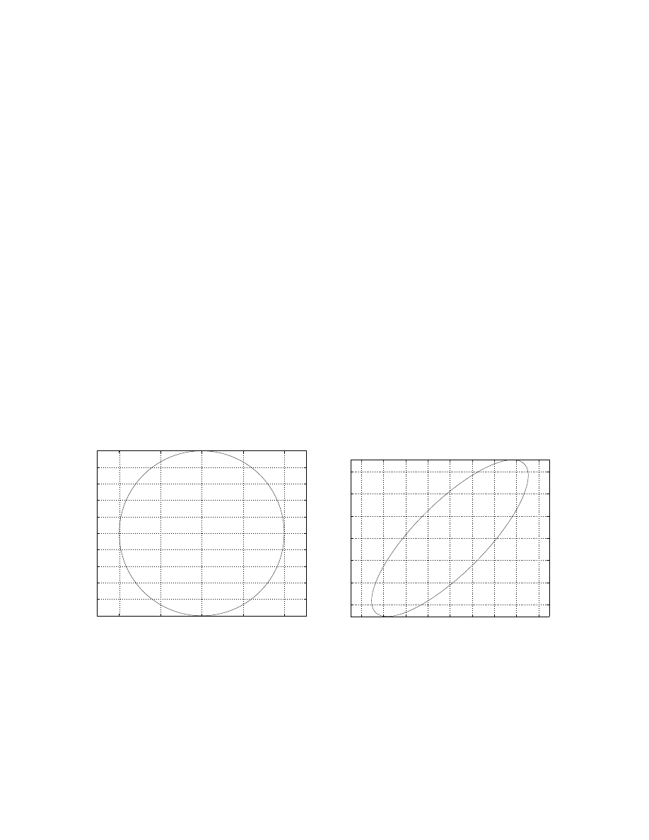
The phase plot for x

∗

(t) is given by Fig. 8-(a), while that for x(t) is given by Fig.

8-(b).

-1

-0.5

0

0.5

1

-1

-0.8

-0.6

-0.4

-0.2

0

0.2

0.4

0.6

0.8

1

x*1

x*2

-0.8

-0.6

-0.4

-0.2

0

0.2

0.4

0.6

0.8

-0.6

-0.4

-0.2

0

0.2

0.4

0.6

x1

x2

(a) ˙x

∗

= J

c

x

∗

(b) ˙x = Ax

Figure 8: Phase plots

22.6

Problems

1. Find (by hand calculation) the eigenvalues and eigenvectors of the matrix

A =







−3 −2

2

5

7

−5

5

8

−6







194

Does e

At

have all of its terms decaying to zero?

2. Read about the MatLab command eig (use the MatLab manual, the Matlab

primer, and/or the comnand >> help eig). Repeat problem 1 using eig,
and explain any differences that you get. If a matrix has distinct eigenvalues,
in what sense are the eigenvectors not unique?

3. Consider the differential equation ˙x(t) = Ax(t), where x(t) is (3 × 1) and A

is from problem (1) above. Suppose that the initial condition is

x(0) =







1

−1

0







Write the initial condition as a linear combination of the eigenvectors, and
find the solution x(t) to the differential equation, written as a time-dependent,
linear combination of the eigenvectors.

4. Suppose that we have a 2nd order system (x(t) ∈ R

2

) governed by the

differential equation

˙x(t) =

"

0 −2
2 −5

#

x(t)

Let A denote the 2 × 2 matrix above.

(a) Find the eigenvalues an eigenvectors of A. In this problem, the eigen-

vectors can be chosen to have all integer entries (recall that eigenvectors
can be scaled)

195

(b) On the grid below (x

1

/x

2

space), draw the eigenvectors.

-

-

-

-

-

-

-

-

-

-

6 6 6 6 6

6 6 6 6 6

6

-

x

1

x

2

(c) A plot of x

2

(t) vs. x

1

(t) is called a phase-plane plot. The variable t is

not explicitly plotted on an axis, rather it is the parameter of the tick
marks along the plot. On the grid above, using hand calculations, draw
the solution to the equation ˙x(t) = Ax(t) for the initial conditions

x(0) =

"

3
3

#

,

x(0) =

"

−2

2

#

,

x(0) =

"

−3
−3

#

,

x(0) =

"

4
2

#

HINT: Remember that if v

i

are eigenvectors, and λ

i

are eigenvalues of

A, then the solution to ˙x(t) = Ax(t) from the initial condition x(0) =

P

2

i=1

α

i

v

i

is simply

x(t) =

n

X

i=1

α

i

e

λ

i

t

v

i

(d) Use Matlab to create a similar picture with many (say 20) different

initial conditions spread out in the x

1

, x

2

plane

5. Suppose A is a real, n

× n matrix, and λ is an eigenvalue of A, and λ is not

real, but λ is complex. Suppose v ∈ C

n

is an eigenvector of A associated

with this eigenvalue λ. Use the notation λ = λ

R

+ jλ

I

and v = v

r

+ jv

I

for

the real and imaginary parts of λ, and v ( j means

√

−1).

(a) By equating the real and imaginary parts of the equation Av = λv, find

two equations that relate the various real and imaginary parts of λ and
v.

(b) Show that ¯

λ (complex conjugate of λ) is also an eigenvalue of A. What

is the associated eigenvector?

196

(c) Consider the differential equation ˙x = Ax for the A described above,

with the eigenvalue λ and eigenvector v. Show that the function

x(t) = e

λ

R

t

[cos (λ

I

t) v

R

− sin (λ

I

t) v

I

]

satisfies the differential equation. What is x(0) in this case?

(d) Fill in this sentence: If A has complex eigenvalues, then if x(t) starts

on the

part of the eigenvector, the solution x(t) oscillates

between the

and

parts of the eigenvector,

with frequency associated with the

part of the eigenvalue.

During the motion, the solution also increases/decreases exponentially,
based on the

part of the eigenvalue.

(e) Consider the matrix A

A =

"

1

2

−2 1

#

It is possible to show that

A

"

1

√

2

1

√

2

j

1

√

2

−j

1

√

2

#

=

"

1

√

2

1

√

2

j

1

√

2

−j

1

√

2

# "

1 + 2j

0

0

1 − 2j

#

Sketch the trajectory of the solution x(t) in R

2

to the differential equa-

tion ˙x = Ax for the initial condition x(0) =

"

1
0

#

.

(f) Find e

At

for the A given above. NOTE: e

At

is real whenever A is real.

See the notes for tricks in making this easy.

6. A hoop (of radius R) is mounted vertically, and rotates at a constant angular

velocity Ω. A bead of mass m slides along the hoop, and θ is the angle that
locates the bead location. θ = 0 corresponds to the bead at the bottom of
the hoop, while θ = π corresponds to the top of the hoop.

The nonlinear, 2nd order equation (from Newton’s law) governing the bead’s

197

motion is

mR¨

θ + mg sin θ + α ˙θ − mΩ

2

R sin θ cos θ = 0

All of the parameters m, R, g, α are positive.

(a) Let x

1

(t) := θ(t) and x

2

(t) := ˙θ(t). Write the 2nd order nonlinear

differential equation in the state-space form

˙x

1

(t) = f

1

(x

1

(t), x

2

(t))

˙x

2

(t) = f

2

(x

1

(t), x

2

(t))

(b) Show that ¯

x

1

= 0, ¯

x

2

= 0 is an equilibrium point of the system.

(c) Find the linearized system

˙δ

x

(t) = Aδ

x

(t)

which governs small deviations away from the equilibrium point (0, 0).

(d) Under what conditions (on m, R, Ω, g) is the linearized system stable?

Under what conditions is the linearized system unstable?

(e) Show that ¯

x

1

= π, ¯

x

2

= 0 is an equilibrium point of the system.

(f) Find the linearized system ˙δ

x

(t) = Aδ

x

(t) which governs small devia-

tions away from the equilibrium point (π, 0).

(g) Under what conditions is the linearized system stable? Under what

conditions is the linearized system unstable?

(h) It would seem that if the hoop is indeed rotating (with angular velocity

Ω) then there would other equilibrium point (with 0 < θ < π/2). Do
such equilibrium points exist in the system? Be very careful, and please
explain your answer.

(i) Find the linearized system ˙δ

x

(t) = Aδ

x

(t) which governs small devia-

tions away from this equilibrium point.

(j) Under what conditions is the linearized system stable? Under what

conditions is the linearized system unstable?

198

23

Jordan Form

23.1

Motivation

In the last section, we saw that if A ∈ F

n×n

has distinct eigenvalues, then there

exists an invertible matrix T ∈ C

n×n

such that T

−1

AT is diagonal. In this sense,

we say that A is diagonalizable by similarity transformation (the matrix
T

−1

AT is called a similarity transformation of A).

Even some matrices that have repeated eigenvalues can be diagonalized. For in-
stance, take A = I

2

. Both of the eigenvalues of A are at λ = 1, yet A is diagonal

(in fact, any invertible T makes T

−1

AT diagonal).

On the other hand, there are other matrices that cannot be diagonalized. Take,
for instance,

A =

"

0 1
0 0

#

The characteristic equation of A is p

A

(λ) = λ

2

. Clearly, both of the eigenvalues of

A are equal to 0. Hence, if A can be diagonalized, the resulting diagonal matrix
would be the 0 matrix (recall that if A can be diagonalized, then the diagonal
elements are necessarily roots of the equation p

A

(λ) = 0). Hence, there would be

an invertible matrix T such that T

−1

AT = 0

2×2

. Rearranging gives

"

0 1
0 0

# "

t

11

t

12

t

21

t

22

#

=

"

t

11

t

12

t

21

t

22

# "

0 0
0 0

#

Multiplying out both sides gives

"

t

21

t

22

0

0

#

=

"

0 0
0 0

#

But if t

21

= t

22

= 0, then T is not invertible. Hence, this 2 × 2 matrix A cannot

be diagonalized with a similarity transformation.

23.2

Details

It turns out that every matrix can be “almost” diagonalized using similarity trans-
formations. Although this result is not difficult to prove, it will take us too far
from the main flow of the course. The proof can be found in any decent linear
algebra book. Here we simply outline the facts.

199

Definition: If J ∈ C

m×m

appears as

J =



















λ 1

0

· · · 0

0 λ

1

· · · 0

. .. ...

λ

1

0 0

0

· · · λ



















then J is called a Jordan block of dimension m, with associated eigenvalue λ.

Theorem: (Jordan Canonical Form) For every A ∈ F

n×n

, there exists an invertible

matrix T ∈ C

n×n

such that

T

−1

AT =













J

1

0

· · · 0

0

J

2

· · · 0

... ... ... ...

0

0

· · · J

k













where each J

i

is a Jordan block.

If J ∈ F

m×m

is a Jordan block, then using the power series definition, it is straight-

forward to show that

e

Jt

=

















e

λt

te

λt

· · ·

t

m−1

(m−1)!

e

λt

0

e

λt

. ..

t

m−2

(m−2)!

e

λt

...

... ...

...

0

0

· · ·

e

λt

















Note that if Re (λ) < 0, then every element of e

Jt

decays to zero, and if if Re (λ) ≥

0, then some elements of e

Jt

diverge to ∞.

23.3

Significance

In general, there is no numerically reliable way to compute the Jordan form of a
matrix. It is a conceptual tool, which, among other things, shows us the extent to
which e

At

contains terms other than exponentials.

Notice that if the real part of λ is negative, then for any finite integer m,

lim

t→∞

n

t

m

e

λt

o

= 0 .

From this result, we see that even in the case of Jordan blocks, the signs of the
real parts of the eigenvalues of A determine the stability of the linear differential
equation

˙x(t) = Ax(t)

200