arXiv:math.MG/0001097 v1 18 Jan 2000

Drawing with Complex Numbers

Michael Eastwood

♯

and Roger Penrose

It is not commonly realized that the algebra of complex numbers can be

used in an elegant way to represent the images of ordinary 3-dimensional
figures, orthographically projected to the plane. We describe these ideas
here, both using simple geometry and setting them in a broader context.

Consider orthogonal projection in Euclidean n-space onto an m-dimen-

sional subspace. We may as well choose co¨ordinates so that this is the
standard projection P : R

n

→ R

m

onto the first m variables. Fix a non-

degenerate simplex Σ in R

n

. Two such simplices are said to be similar if

one can be obtained from the other by a Euclidean motion together with
an overall scaling. This article answers the following question. Given n + 1
points in R

m

, when can these points be obtained as the images under P of

the vertices of a simplex similar to Σ?

When n = 3 and m = 2, then P is the standard orthographic projection

(as often used in engineering drawing) and we are concerned with how to
draw a given tetrahedron. We shall show, for example, that four points
α, β, γ, δ in the plane are the orthographic projections of the vertices of a
regular tetrahedron if and only if

(α + β + γ + δ)

2

= 4(α

2

+ β

2

+ γ

2

+ δ

2

)

(1)

where α, β, γ, δ are regarded as complex numbers! Similarly, suppose a cube
is orthographically projected and normalised so that a particular vertex is
mapped to the origin. If α, β, γ are the images of the three neighbouring
vertices, then

α

2

+ β

2

+ γ

2

= 0,

(2)

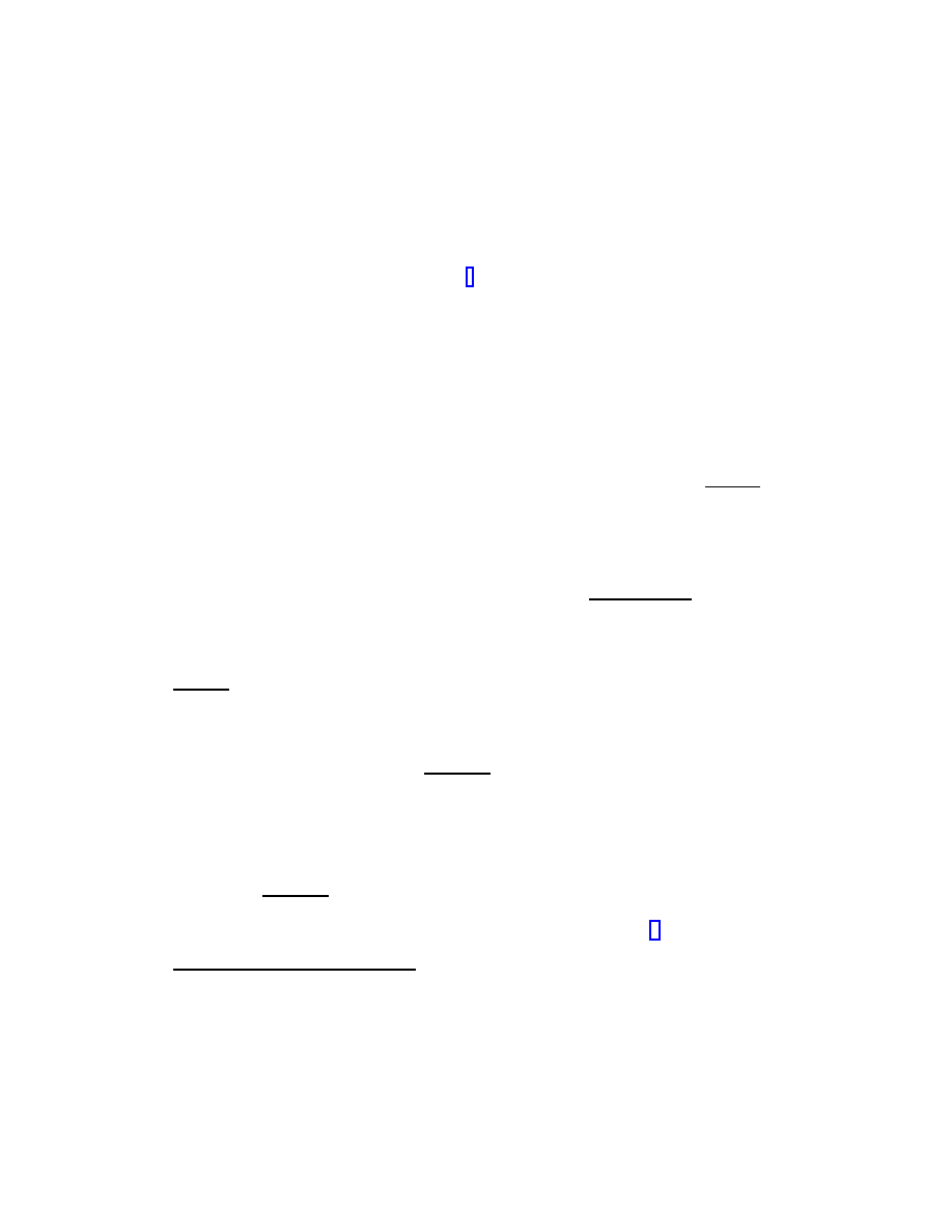
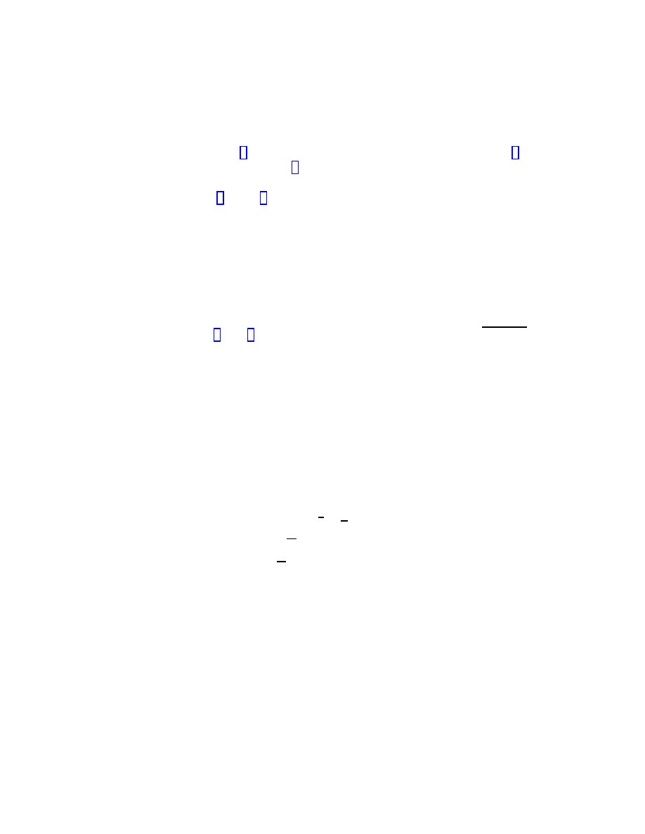
again as a complex equation. Conversely, if this equation is satisfied, then
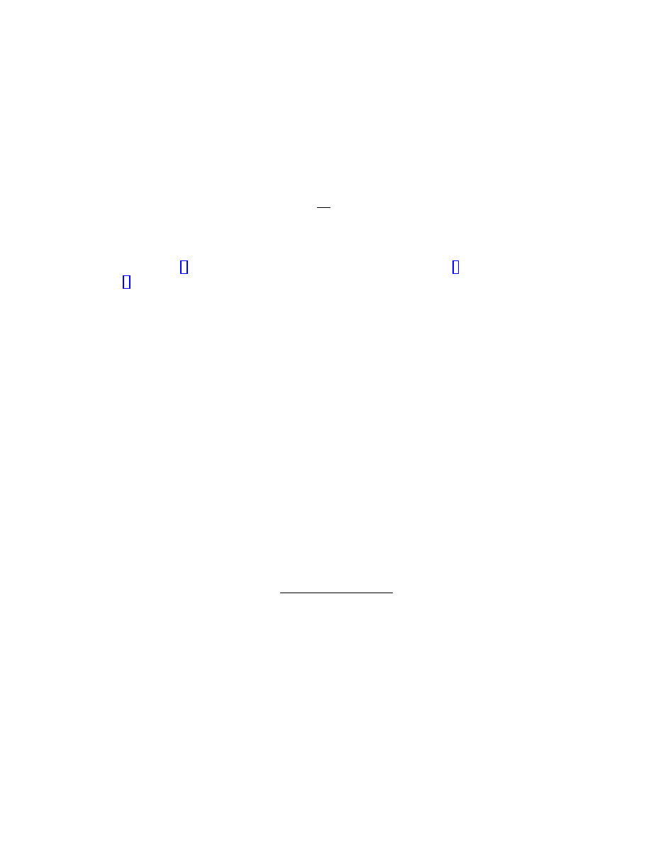
one can find a cube whose orthographic image is given in this way. Since
parallel lines are seen as parallel in the drawing, equation (2) allows one to
draw the general cube:

♯

Supported by the Australian Research Council.

1

γ

β

α

0

In this example, α = 2 − 26i

β = −23 + 2i
γ = 14 + 7i

The result for a cube is known as Gauss’ fundamental theorem of

axonometry—see [3, p. 309] where it is stated without proof. In engineer-
ing drawing, one usually fixes three principal axes in Euclidean three-space
and then an orthographic projection onto a plane transverse to these axes
is known as an axonometric projection (see, for example, [8, Chapter 17]).
Gauss’ theorem may be regarded as determining the degree of foreshortening
along the principal axes for a general axonometric projection. The projec-
tion corresponding to taking α, β, γ to be the three cube roots of unity is
called isometric projection because the foreshortening is the same for the
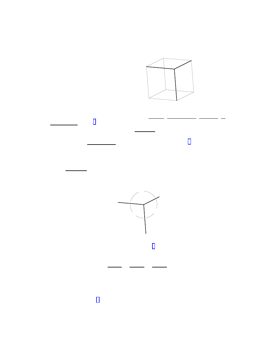
three principal axes. In an axonometric drawing, it is conventional to take
the image axes at mutually obtuse angles:

A

B

C

If |α| = a, |β| = b, |γ| = c, then equation (2) is equivalent to the sine rule
for the triangle with sides α

2

, β

2

, γ

2

, namely

a

2

sin 2A

=

b

2

sin 2B

=

c

2

sin 2C

.

In this form, the fundamental theorem of axonometry is due to Weisbach and
was published in T¨

ubingen in 1844 in the Polytechnische Mitteilungen of Volz

and Karmasch. Equivalent statements can be found in modern engineering
drawing texts (e.g. [7, p. 44]).

2

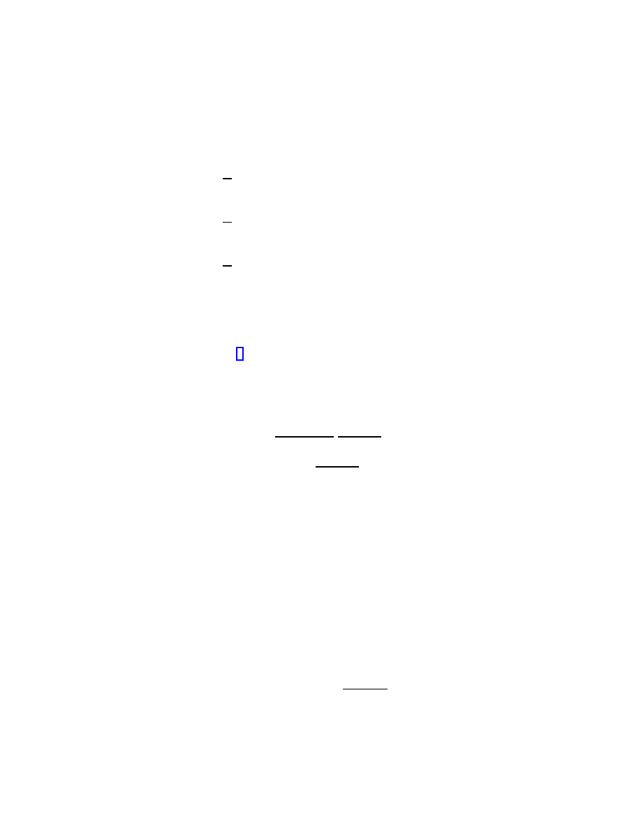
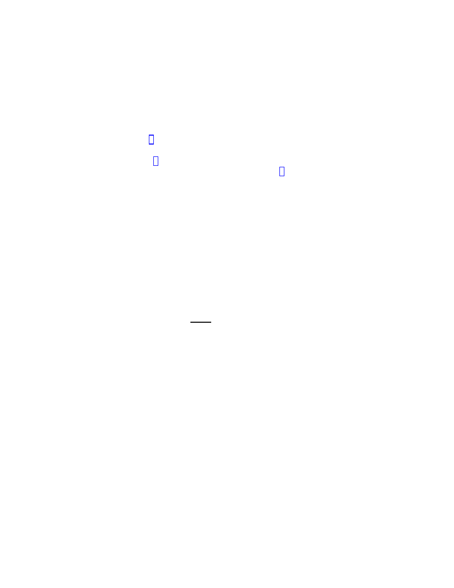
Equation (2) may be used to give a ruler and compass construction of

the general orthographic image of a cube. If we suppose that the image of a
vertex and two of its neighbours are already specified, then (2) determines (up
to a two-fold ambiguity) the image of the third neighbour. The construction
is straightforward except perhaps for the construction of a complex square
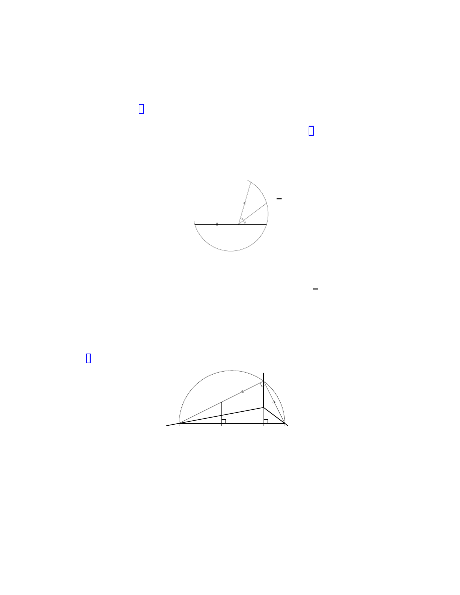
root for which we advocate the following as quite efficient:

z

√

z

0

1

ζ

•

•

•

•

•

Firstly ζ is constructed by marking the real axis at a distance kzk from the
origin. Then, a circle is constructed passing through the three points ζ, 1,
and z. Finally, the angle between 1 and z is bisected and

√

z appears where

this bisector meets the circle.

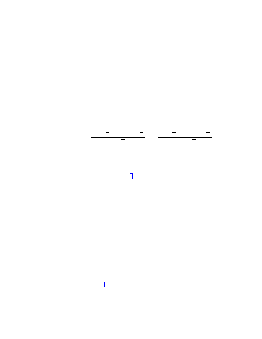
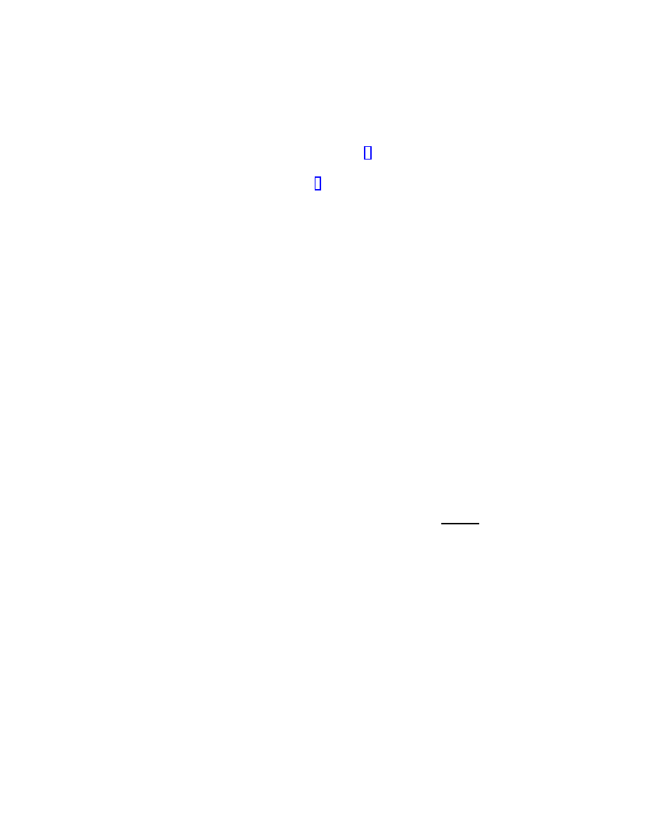
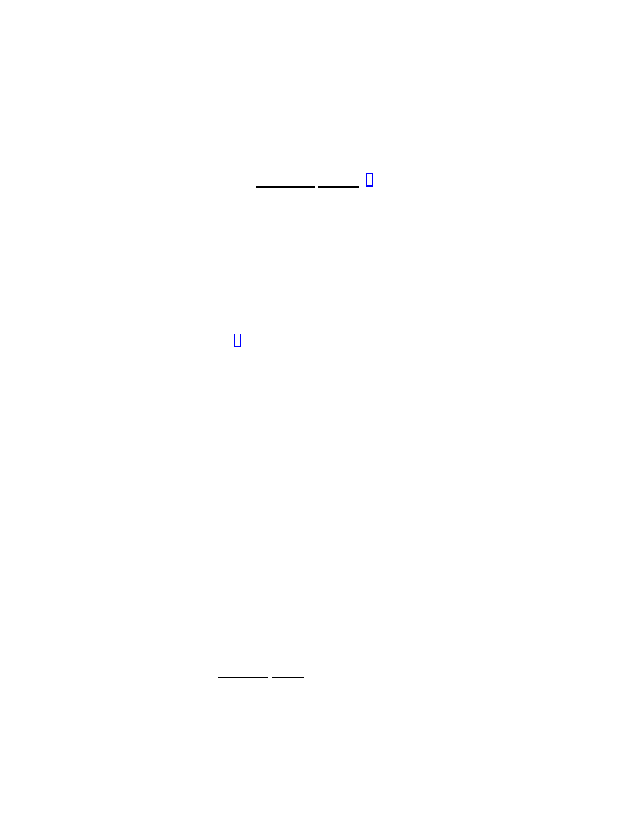
In engineering drawing, it is more usual that the images of the three

principal axes are prescribed or chosen by the designer and one needs to
determine the relative degree of foreshortening along these axes. There is a
ruler and compass construction given by T. Schmid in 1922 (see, for example,
[8, §17.17–17.19]):

α

β

P

Q

R

0

•

•

•

•

•

•

In this diagram, the three principal axes and α are given. By drawing a
perpendicular from α to one of the of the principal axes and marking its
intersection with the remaining principal axis, we obtain P . The point Q
is obtained by drawing a semi-circle as illustrated. The point R is on the
resulting line and equidistant with α from Q. Finally, β is obtained by
dropping a perpendicular as shown. It is easy to see that this construction has

3

the desired effect—in Euclidean three-space rotate the right-angled triangle
with hypotenuse P α about this hypotenuse until the point Q lies directly
above 0 in which case R will lie directly above β and the third vertex will lie
somewhere over the line through 0 and Q. One may verify the appropriate
part of Weisbach’s condition

a

2

sin 2A

=

b

2

sin 2B

(3)

by the following calculation. Without loss of generality we may represent
all these points by complex numbers normalised so that Q = 1. Then it is
straightforward to check that

R = 1 + i − iα, P =

α(α + α) + 2(1

− α − α)

α − α

, β =

α(α + α) + 2(1 − α − α)

2 − α − α

i

and therefore that

α

2

+ β

2

= 4

(α − 1)(α − 1)(α + α − 1)

(α + α − 2)

2

.

That α

2

+ β

2

is real is equivalent to (3).

To prove Gauss’ theorem more directly consider three vectors in R

3

as the

columns of a 3 × 3 matrix. This matrix is orthogonal if and only if the three
vectors are orthonormal. It is equivalent to demand that the three rows be
orthonormal. However, any two orthonormal vectors in R

3

may be extended

to an orthonormal basis. Thus, the condition that three vectors









x

1

y

1

















x

2

y

2

















x

3

y

3









in R

2

be the images under P : R

3

→ R

2

of an orthonormal basis of R

3

, is

that





x

1

x

2

x

3





and





y

1

y

2

y

3





be orthonormal in R

3

. Dropping the overall scale, we obtain

x

1

2

+ x

2

2

+ x

3

2

= y

1

2

+ y

2

2

+ y

3

2

and

x

1

y

1

+ x

2

y

2

+ x

3

y

3

= 0.

Writing, α = x

1

+iy

1

, β = x

2

+y

2

, γ = x

3

+y

3

, these two equations are the real

and imaginary parts of (2). To deduce the case of a regular tetrahedron as

4

described by equation (1) from the case of a cube as described by equation (2),
it suffices to note that equation (1) is translation invariant and that a regular
tetrahedron may be inscribed in a cube. Thus, we may take δ = α + β + γ
and observe that (1) and (2) are then equivalent.

It is easy to see that the possible images of a particular tetrahedron Σ in

R

3

under an arbitrary Euclidean motion followed by the projection P form

a 5-dimensional space—the group of Euclidean motions is 6-dimensional but
translation orthogonal to the plane leaves the image unaltered. It therefore
has codimension 3 in the 8-dimensional space of all tetrahedral images (2 de-
grees of freedom for each vertex). Allowing similar tetrahedra rather than
congruent reduces the codimension to 2. Therefore, two real equations are to
be expected. Always, these two real equations combine as a single complex
equation such as (1) or (2). At first sight, this is perhaps surprising and even
more so when the same phenomenon occurs for P : R

n

→ R

2

for arbitrary n.

For n = 3, there is a proof of Gauss’ theorem which brings in complex

numbers at the outset. Consider the space H of Hermitian 2 × 2 matrices
with zero trace, i.e. matrices of the form

X =









w

u + iv

u − iv

−w









for















u
v

w















∈ R

3

.

We may identify H with R

3

and, in so doing, − det X becomes the square of

the Euclidean length. The group G of invertible 2 × 2 complex matrices of
the form

Λ =







a −b

b

a







acts linearly on H by X 7→ ΛXΛ

t

. Moreover,

det(ΛXΛ

t

) = (|a|

2

+ |b|

2

)

2

det X

so G acts by similarities. It is easy to check that all similarities may be
obtained in this way. (This trick is essentially as used in Hamilton’s theory
of quaternions and is well known to physicists—in modern parlance it is
equivalent to the isomorphism of Lie groups Spin(3) ∼

= SU(2).) Therefore,

an arbitrary orthographicimage of a cube may be obtained by acting with Λ
on the standard basis









0 1
1 0







 ,









0

i

−i 0







 ,









1

0

0 −1









5

and then picking out the top right hand entries. We obtain

Λ









0 1
1 0







 Λ

t

=









∗ a

2

− b

2

∗

∗









7−→ a

2

− b

2

= α

Λ









0

i

−i 0







 Λ

t

=









∗ i(a

2

+ b

2

)

∗

∗









7−→ i(a

2

+ b

2

) = β

Λ









1

0

0 −1







 Λ

t

=









∗ 2ab
∗

∗









7−→ 2ab

= γ

and therefore α

2

+ β

2

+ γ

2

= 0, as required. Conversely, this is exactly the

condition that α, β, γ may be written in this form. (Compare the half angle
formulae—if s

2

+ c

2

= 1, then s = 2t/(1 + t

2

) and c = (1 − t

2

)/(1 + t

2

) for

some t.) That Gauss [3, p. 309] makes the same observation concerning the
form of α, β, γ suggests that perhaps he also had this reasoning in mind.

The proof of Gauss’ theorem using orthogonal matrices clearly extends

to P : R

n

→ R

2

= C for arbitrary n. To state it, the following terminology

concerning the standard projection P : R

n

→ R

m

is useful. We shall say

that v

1

, v

2

, . . . , v

n

∈ R

m

are normalised eutactic if and only if there is an

orthonormal basis u

1

, u

2

, . . . , u

n

of R

n

with v

j

= P u

j

for j = 1, 2, . . . , n. We

shall say that v

1

, v

2

, . . . , v

n

∈ R

m

are eutactic if and only if µv

1

, µv

2

, . . . , µv

n

are normalised eutactic for some µ 6= 0.

Theorem The points z

1

, z

2

, . . . , z

n

∈ C = R

2

are eutactic if and only if

z

1

2

+ z

2

2

+ · · · + z

n

2

= 0

and not all

z

j

are zero.

There is a proof for n = 4 based on the isomorphism

Spin(4) ∼

= SU(2)

× SU(2)

and, indeed, this is how we came across the theorem in the first place. How-
ever, a more direct route to complex numbers and one which applies in all
dimensions is based on the observation that Gr

+
2

(R

2

), the Grassmannian of

oriented two-planes in R

n

, is naturally a complex manifold. When n = 3,

6

this Grassmannian is just the two-sphere and has a complex structure as the
Riemann sphere. In general, consider the mapping

CP

n−1

\ RP

n−1

π

−→ Gr

+
2

(R

n

)

induced by C

n

∋ z 7→ iz∧z. In other words, a complex vector z = x+iy ∈ C

n

is mapped to the two-dimensional oriented subspace of R

n

spanned by x and

y, the real and imaginary parts of z. Let h , i denote the standard inner
product on R

n

extended to C

n

as a complex bilinear form. Then, hz, zi = 0

imposes two real equations

kxk

2

= kyk

2

and hx, yi = 0

on the real and imaginary parts. In other words, x, y is proportional to an or-
thonormal basis for span{x, y}. Hence, if z and w satisfy hz, zi = 0 = hw, wi
and define the same oriented two-plane, then w = λz for some λ ∈ C \ {0}.
The non-singular complex quadric

K = {[z] ∈ CP

n−1

s.t. hz, zi = 0}

avoids RP

n−1

⊂ CP

n−1

and we have shown that π|

K

is injective. It is clearly

surjective. The isomorphism

π : K ∼

=

−→ Gr

+
2

(R

n

)

respects the natural action of SO(n) on K and Gr

+
2

(R

n

). The generalised

Gauss theorem follows immediately since, rather than asking about the image
of a general orthonormal basis under the standard projection P : R

n

→ R

2

,

we may, equivalently, ask about the image of the standard basis e

1

, e

2

, . . . , e

n

under a general orthogonal projection onto an oriented two-plane Π ⊂ R

n

.

Any such Π is naturally complex, the action of i being given by rotation by
90

◦

in the positive sense. If Π is represented by [z

1

, z

2

, . . . , z

n

] ∈ K as above

and we use x, y ∈ Π to identify Π with C, then e

j

7→ z

j

and

z

1

2

+ z

2

2

+ · · · + z

n

2

= hz, zi = 0,

as required. Conversely, a solution of this complex equation determines an
appropriate plane Π.

For the case of a general tetrahedron or simplex and for general m and

n, it is more convenient to start with Hadwiger’s theorem [4] or [2, page 251]
as follows. The proof is obtained by extending our orthogonal matrix proof
of Gauss’ theorem.

7

Theorem (Hadwiger) Assemble v

1

, v

2

, . . . , , v

n

∈ R

m

as the columns of an

m×n matrix V . These vectors are normalised eutactic if and only if V V

t

= 1

(the m × m identity matrix).

Proof If v

1

, v

2

, . . . , v

n

are normalised eutactic, then assembling a corre-

sponding orthonormal basis of R

n

as the columns of an n × n matrix, we

have V = P U and U

t

U = 1 (the n × n identity matrix). Therefore, UU

t

= 1

and

V V

t

= P UU

t

P

t

= P P

t

= 1,

as required. Conversely, if V V

t

= 1, then the columns of V

t

may be com-

pleted to an orthonormal basis of R

n

, i.e. V

t

= U

t

P

t

for UU

t

= 1. Now,

U

t

U = 1 and V = P U, as required.

2

The case of a general simplex is obtained essentially by a change of basis

as follows. Suppose a

1

, a

2

, . . . , a

n

, a

n+1

are the vertices of a non-degenerate

simplex Σ in R

n

whose centre of mass is at the origin. In other words, the

n × (n + 1) matrix A has rank n and Ae = 0 where e is the column vector all
of whose n + 1 entries are 1. Form the (n + 1) × (n + 1) symmetric matrix

Q = A

t

(AA

t

)

−2

A,

noting that rank A = n implies the moment matrix AA

t

is invertible.

Theorem Given b

1

, b

2

, . . . , b

n

, b

n+1

∈ R

m

assembled as the columns of an

m×(n+1) matrix B, these vectors are the images under orthogonal projection
P : R

n

→ R

m

of the vertices of a simplex congruent to

Σ if and only if

BQ

t

B = 1.

(4)

Proof The vertices of a simplex congruent to Σ are the columns of a matrix
UA + ae

t

for some orthogonal matrix U and translation vector a ∈ R

n

. Also,

note that Qe = 0. Thus, if B = P (UA + ae

t

), then

BQB

t

= P UAQA

t

U

t

P

t

= P UAA

t

(AA

t

)

−2

AA

t

U

t

P

t

= P UU

t

P

t

= P P

t

= 1,

8

as required. Conversely, Qe = 0 implies that (4) is translation invariant. So,
without loss of generality, we may suppose that b

1

+ b

2

+ · · · + b

n

+ b

n+1

= 0,

that is to say, Be = 0. Writing out (4) in full gives

BA

t

(AA

t

)

−1

(BA

t

(AA

t

)

−1

)

t

= 1

so, by Hadwiger’s theorem, there is an orthogonal matrix U so that

BA

t

(AA

t

)

−1

= P U.

Thus,

BA

t

(AA

t

)

−1

A = P UA

and

Be = 0.

Certainly, B = P UA is a solution of these equations but it is the only
solution since A

t

(AA

t

)

−1

A has rank n and e is not in the range of this linear

transformation.

2

Corollary (case m = 2) Points z

1

, z

2

, . . . , z

n

, z

n+1

∈ C are the images un-

der orthogonal projection of the vertices of a simplex similar to

Σ if and only

if

z

t

Qz = 0

where

z is the column vector with components z

1

, z

2

, . . . , z

n

, z

n+1

.

It is, of course, possible to compute Q explicitly for any given example. If

the simplex Σ has some degree of symmetry, however, we can often circum-
vent such computation. Consider, for example, the case of a regular simplex.
From the corollary above, we know that the image of such a simplex in the
plane is characterised by a complex homogeneous quadratic polynomial. The
symmetries of the regular simplex ensure that this polynomial must be in-
variant under S

n+1

, the symmetric group on n + 1 letters. Hence, it must be

expressible in terms of the elementary symmetric polynomials. Equivalently,
it must be a linear combination of

(z

1

+ z

2

+ · · · + z

n

+ z

n+1

)

2

and

z

1

2

+ z

2

2

+ · · · + z

n

2

+ z

n+1

2

.

Up to scale, there is only one such combination which is translation invariant,
namely

(z

1

+ z

2

+ · · · + z

n

+ z

n+1

)

2

− (n + 1)(z

1

2

+ z

2

2

+ · · · + z

n

2

+ z

n+1

2

).

(5)

9

It follows that the vanishing of this polynomial is an equation which charac-
terises the possible images of a regular simplex under orthogonal projection
into the plane. The special case n = 2 characterises the equilateral triangles
in the plane [1, Problem 15 on page 79].

Equation (2) characterising the orthographic images of a cube, may be

deduced by similar symmetry considerations. If a particular vertex is mapped
to the origin and its neighbours are mapped to α, β, γ then, since each of these
neighbouring vertices is on an equal footing, the polynomial in question must
be a linear combination of (α + β + γ)

2

and α

2

+ β

2

+ γ

2

. To find out which

linear combination we need only consider a particular projection, for example:

•

•

•

γ = i

β = 1

α = 0

In this example, (α + β + γ)

2

= 2i and α

2

+ β

2

+ γ

2

= 0. Up to scale,

therefore, (2) is the correct equation.

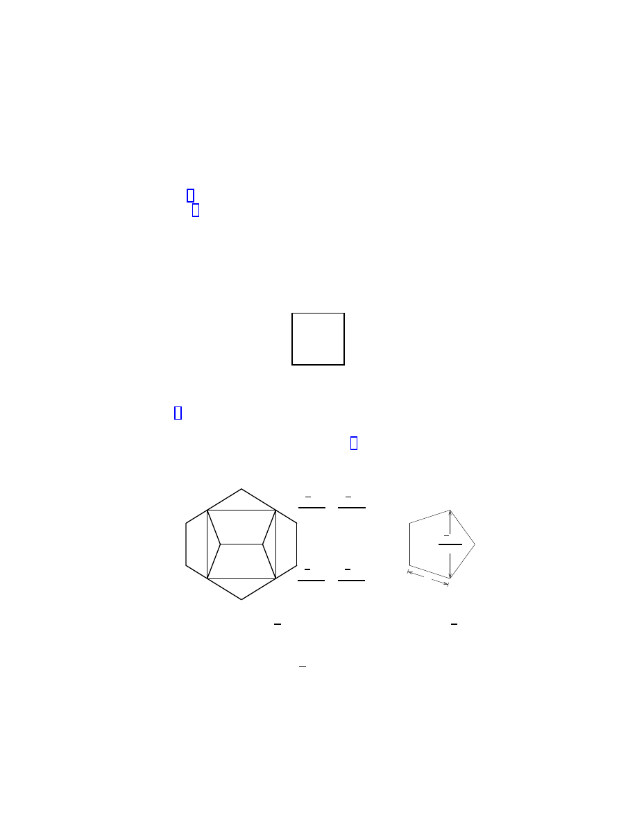
The case of a regular dodecahedron is similar. Using the fact that a cube

may be inscribed in such a dodecahedron [5], we may deduce a particular
projection:

•

•

•

•

0

β = −1

γ =

√

5

− 1

4

−

√

5 + 1

4

i

α =

√

5

− 1

4

+

√

5 + 1

4

i

1

√5 + 1

2

with (α + β + γ)

2

= (7 − 3

√

5)/2 and α

2

+ β

2

+ γ

2

= (2 −

√

5)/2. In this

particular case,

(α + β + γ)

2

+ (

√

5 − 1)(α

2

+ β

2

+ γ

2

) = 0.

10

Therefore, this is the correct equation in the general case. It may be used
as the basis of a ruler and compass construction of the general orthographic
projection of a regular dodecahedron.

It is interesting to note that if all the vertices of a Platonic solid are

orthographically projected to z

1

, z

2

, . . . , z

N

∈ C, then

(z

1

+ z

2

+ · · · + z

N

)

2

= N(z

1

2

+ z

2

2

+ · · · + z

N

2

)

(6)

(compare (5)).

For a tetrahedron, this is just equation (1).

To verify

(6) for the other Platonic solids, firstly note that it is translation invari-
ant. Therefore, it suffices to impose z

1

+ z

2

+ · · · + z

N

= 0 and show that

z

1

2

+z

2

2

+· · ·+z

N

2

= 0. The case of a cube now follows immediately since its

vertices may be grouped as two regular tetrahedra. The dodecahedral case
may be dealt with by grouping its vertices into five regular tetrahedra. The
regular octahedron is amenable to a similar trick but not the icosahedron.
Rather than resorting to direct computation, a uniform proof may be given as
follows. As before, assemble the vertices of the given solid Σ as the columns
of a matrix A, now of size 3 ×N, and consider the moment matrix M ≡ AA

t

.

Observe that





1 i 0





M















1

i

0















= z

1

2

+ z

2

2

+ · · · + z

N

2

.

The moment matrix is positive definite and symmetric. In other words, it
defines a metric on R

3

, manifestly invariant under the symmetries of Σ. If Σ

is regular—or, more generally, enjoys the symmetries of a regular solid (e.g. a
cuboctahedron or rhombicosidodecahedron)—then its symmetry group acts
irreducibly on R

3

. Thus, M must be proportional to the identity matrix and

the result follows. For a general solid Σ, the two complex numbers

±

p

z

1

2

+ z

2

2

+ · · · + z

N

2

are the foci of the ellipse





x y





R









x
y







 = 1

where R is the inverse of the quadratic form obtained by restricting M to the
plane of projection.

11

This reasoning also works in higher dimensions where it shows (as con-

jectured to us by H.S.M. Coxeter) that the orthogonally projected images
in the plane of the N vertices of any regular polytope, real or complex, will
satisfy equation (6). Of course, this excludes regular polygons (whose sym-
metry groups act reducibly except in dimension two) orthographic images of
which will satisfy (6) if and only if the image is itself regular. For polyhedra
other than simplices, a quadratic equation such as (6) is no longer sufficient
to characterise the orthogonal image up to scale. In general, there will also
be some linear relations. For a non-degenerate N-gon there will be N − n − 1
such relations. The simplest example is a square in R

2

which is characterised

by the complex equations

(α + β + γ + δ)

2

= 4(α

2

+ β

2

+ γ

2

+ δ

2

)

and

α + γ = β + δ.

It is interesting to investigate further the relationship between a non-

degenerate simplex Σ in R

n

and its quadratic form Q = A

t

(AA

t

)

−2

A. Recall

that A is the n × (n + 1) matrix whose columns are the vertices of Σ. There
are several other formulae for or characterisations of Q. Let S denote the
(n + 1) × (n + 1) symmetric matrix

1

−

1

n + 1



























1 1 · · · 1
1 1 · · · 1

..

.

..

.

. .. ...

1 1 · · · 1



























.

It is the matrix of orthogonal projection in R

n+1

in the direction of the

vector e. We maintain that Q is characterised by the equations

QA

t

A = S

and

Qe = 0.

Certainly, if these equations hold, then they are enough to determine Q
because the moment matrix M ≡ A

t

A has rank n and e is not in its range.

The second equation is evident and the first equation with Q replaced by
A

t

(AA

t

)

−2

A and simplified reads

A

t

(AA

t

)

−1

A = S.

To see that this holds it suffices to observe that it is clearly true after post-
multiplication by A

t

or e. We may equally well characterise Q by means of

the equations

A

t

AQ = S

and

Qe = 0.

12

These equations relate M and Q geometrically—both matrices annihilate e
whilst on the hyperplane orthogonal to e they are mutually inverse. This
implies that M and Q are generalised inverses [6] of each other. Thus,

Q = M

†

= (A

t

A)

†

= A

†

A

†t

where A

†

is the generalised inverse of A. In this case, A

†

= A

t

(AA

t

)

−1

. This

also shows how to compute Q more directly in certain cases. The moment
matrix M has direct geometric interpretation as the various inner products of
the vectors a

1

, a

2

, . . . , a

n

, a

n+1

. In the case of a regular simplex, for example,

we know that ka

i

k

2

is independent of i, that ka

i

− a

j

k

2

is independent of

i 6= j, and that a

1

+ a

2

+ . . . + a

n

+ a

n+1

= 0. We may deduce that, with a

suitable overall scale, M = S. Since S

†

= S, it follows that Q = S. This is

a direct derivation of (5).

It is clear geometrically that M or, equivalently, Q determines Σ up to

congruency. Alternatively, one can argue algebraically—it is easy to check
that if A

t

A = B

t

B, then U = AA

t

(BA

t

)

−1

is orthogonal and A = UB.

Therefore, the possible quadratic forms Q which can arise give a natural
parametrisation of the non-degenerate simplices up to congruency. Choosing
a basepoint Σ

0

with corresponding matrix A

0

, and mapping X ∈ GL(n, R)

to X

−1

A

0

identifies the space of non-degenerate simplices up to congruency

with the homogeneous space GL(n, R)/O(n). This homogeneous space may
also be identified with the space of positive definite n × n quadratic forms
by sending X ∈ GL(n, R) to XX

t

. The (n + 1) × (n + 1) quadratic form Q

corresponding to X

−1

A

0

is given by A

†
0

XX

t

A

†t
0

. It follows that the general

Q which can arise is characterised by the following two conditions:

• Qe = 0 and only multiples of e are in the kernel of Q.

• All other eigenvalues of Q are positive.

It is also possible to repeat this analysis in pseudo-Euclidean spaces. The
only difference is that the condition that the non-zero eigenvalues of Q be
positive is replaced by a condition on sign precisely reflecting the original
signature of the inner product.

Finally we should mention some possible applications. There is much

current interest in computer vision. In particular, there is the problem of
recognising a wire-frame object from its orthographic image. The results we

13

have described can be used as test on such an image, for example to see
whether a given image could be that of a cube or to keep track of a moving
shape. It is clear that such tests could be implemented quite efficiently. An-
other possibility is in the manipulation of CADD

♯

data. Rather than storing

an image as an array of vectors in R

3

, it may be sometimes be more efficient to

store certain tetrahedra within such an image by means of the corresponding
quadratic form. For orthographic imaging this may be preferable.

We would like to thank H.S.M. Coxeter for drawing our attention to

Hadwiger’s article, R. Michaels and J. Cofman for pointing out Gauss’ and
Weisbach’s work, and E.J. Pitman for many useful conversations.

References

[1] S. Barnard and J.M. Child, Higher Algebra, MacMillan 1936.

[2] H.S.M. Coxeter, Regular Polytopes, Methuen 1948.

[3] C.F. Gauss, Werke, Zweiter Band, K¨

oniglichen Gesellschaft der Wis-

senschaften, G¨

ottingen 1876.

[4] H. Hadwiger, ¨

Uber ausgezeichnete Vectorsterne und regul¨

are Polytope

,

Comment. Math. Helv. 13 (1940), 90–108.

[5] D. Hilbert and S. Cohn-Vossen, Geometry and the Imagination, Chelesa

1952, 1983, 1990.

[6] R. Penrose, A generalised inverse for matrices, Proc. Camb. Phil. Soc. 51

(1955), 406–413.

[7] R.N. Roth and I.A. van Haeringen, The Australian Engineering Drawing

Handbook, Part One

, The Institute of Engineers, Australia 1988.

[8] R.P. Hoelscher and C.H. Springer, Engineering Drawing and Geometry,

Second Edition

, Wiley 1961.

Department of Pure Mathematics

Mathematical Institute

University of Adelaide

24-29 Saint Giles’

South AUSTRALIA 5005

Oxford OX1 3LB
ENGLAND

♯

Computer Aided Drafting and Design.

14