
Ciletti, M.D., Irwin, J.D., Kraus, A.D., Balabanian, N., Bickart, T.A., Chan, S.P., Nise,
N.S. “Linear Circuit Analysis”
The Electrical Engineering Handbook
Ed. Richard C. Dorf
Boca Raton: CRC Press LLC, 2000

© 2000 by CRC Press LLC
3
Linear Circuit Analysis
Kirchhoff ’s Current Law • Kirchhoff ’s Current Law in the Complex
Domain • Kirchhoff ’s Voltage Law • Kirchhoff ’s Voltage Law in the
Complex Domain • Importance of KVL and KCL
Node Analysis • Mesh Analysis • Summary
Linearity and Superposition • The Network Theorems of Thévenin
and Norton • Tellegen’s Theorem • Maximum Power Transfer • The
Reciprocity Theorem • The Substitution and Compensation Theorem
Tellegen’s Theorem • AC Steady-State Power • Maximum Power
Transfer • Measuring AC Power and Energy
3.5 Three-Phase Circuits
3.6 Graph Theory
The
k
-Tree Approach • The Flowgraph Approach • The
k
-Tree
Approach Versus the Flowgraph Approach • Some Topological
Applications in Network Analysis and Design
3.7 Two-Port Parameters and Transformations
Introduction • Defining Two-Port Networks • Mathematical
Modeling of Two-Port Networsk via
z
Parameters • Evaluating Two-
Port Network Characteristics in Terms of
z
Parameters • An Example
Finding
z
Parameters and Network Characteristics • Additional Two-
Port Parameters and Conversions • Two Port Parameter Selection
3.1 Voltage and Current Laws
Michael D. Ciletti
Analysis of linear circuits rests on two fundamental physical laws that describe how the voltages and currents
in a circuit must behave. This behavior results from whatever voltage sources, current sources, and energy
storage elements are connected to the circuit. A voltage source imposes a constraint on the evolution of the
voltage between a pair of nodes; a current source imposes a constraint on the evolution of the current in a
branch of the circuit. The energy storage elements (capacitors and inductors) impose initial conditions on
currents and voltages in the circuit; they also establish a dynamic relationship between the voltage and the
current at their terminals.
Regardless of how a linear circuit is stimulated, every node voltage and every branch current, at every instant
of time, must be consistent with Kirchhoff ’s voltage and current laws. These two laws govern even the most
complex linear circuits. (They also apply to a broad category of nonlinear circuits that are modeled by point
models of voltage and current.)
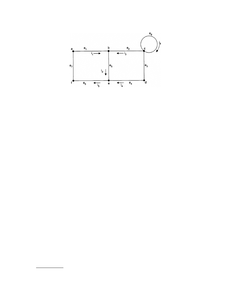
A circuit can be considered to have a topological (or graph) view, consisting of a labeled set of nodes and a
labeled set of edges. Each edge is associated with a pair of nodes. A node is drawn as a
dot
and represents a
Michael D. Ciletti
University of Colorado
J. David Irwin
Auburn University
Allan D. Kraus
Allan D. Kraus Associates
Norman Balabanian
University of Florida
Theodore A. Bickart
Michigan State University
Shu-Park Chan
International Technological
University
Norman S. Nise
California State Polytechnic
University
© 2000 by CRC Press LLC
connection between two or more physical components; an edge is drawn as a
line
and represents a path, or
branch, for current flow through a component (see
The edges, or branches, of the graph are assigned current labels,
i
1
,
i
2
, . . .,
i
m
. Each current has a designated
direction, usually denoted by an
arrow
symbol. If the arrow is drawn toward a node, the associated current is
said to be
entering
the node; if the arrow is drawn away from the node, the current is said to be
leaving
the
node. The current
i
1
is entering node
b
in Fig. 3.1; the current
i
5
is leaving node
e
.
Given a branch, the pair of nodes to which the branch is attached defines the convention for measuring
voltages in the circuit. Given the ordered pair of nodes (
a, b
), a voltage measurement is formed as follows:
v
ab
=
v
a
–
v
b
where
v
a
and
v
b
are the absolute electrical potentials (voltages) at the respective nodes, taken relative to some
reference node. Typically, one node of the circuit is labeled as
ground,
or reference node; the remaining nodes
are assigned voltage labels. The measured quantity,
v
ab
, is called the
voltage drop
from node
a
to node
b
. We
note that
v
ab
= –
v
ba
and that
v
ba
=
v
b
–
v
a
is called the
voltage rise
from
a
to
b
. Each node voltage implicitly defines the voltage drop between the respective
node and the ground node.
The pair of nodes to which an edge is attached may be written as (
a,b
) or (
b,a
). Given an ordered pair of
nodes (
a, b
), a
path from a to b
is a directed sequence of edges in which the first edge in the sequence contains
node label
a
, the last edge in the sequence contains node label
b
, and the node indices of any two adjacent
members of the sequence have at least one node label in common. In Fig. 3.1, the edge sequence {
e
1
,
e
2
,
e
4
} is
not a path, because
e
2
and
e
4
do not share a common node label. The sequence {
e
1
,
e
2
} is a path from node
a
to node
c
.
A path is said to be
closed
if the first node index of its first edge is identical to the second node index of its
last edge. The following edge sequence forms a closed path in the graph given in Fig. 3.1: {
e
1
,
e
2
,
e
3
,
e
4
,
e
6
,
e
7
}.
Note that the edge sequences {
e
8
} and {
e
1
,
e
1
} are closed paths.
Kirchhoff’s Current Law
Kirchhoff ’s current law (KCL) imposes constraints on the currents in the branches that are attached to each
node of a circuit. In simplest terms, KCL states that the sum of the currents that are entering a given node
FIGURE 3.1
Graph representation of a linear circuit.
© 2000 by CRC Press LLC
must equal the sum of the currents that are leaving the node. Thus, the set of currents in branches attached to
a given node can be partitioned into two groups whose orientation is away from (into) the node. The two
groups must contain the same net current. Applying KCL at node
b
in Fig. 3.1 gives
i
1
(
t
) +
i
3
(
t
) =
i
2
(
t
)
A connection of water pipes that has no leaks is a physical analogy of this situation. The net rate at which
water is flowing into a joint of two or more pipes must equal the net rate at which water is flowing away from
the joint. The joint itself has the property that it only connects the pipes and thereby imposes a structure on
the flow of water, but it cannot store water. This is true regardless of when the flow is measured. Likewise, the
nodes of a circuit are modeled as though they cannot store charge. (Physical circuits are sometimes modeled
for the purpose of simulation as though they store charge, but these nodes implicitly have a capacitor that
provides the physical mechanism for
storing
the charge. Thus, KCL is ultimately satisfied.)
KCL can be stated alternatively as: “the algebraic sum of the branch currents entering (or leaving) any node
of a circuit at any instant of time must be zero.” In this form, the label of any current whose orientation is away
from the node is preceded by a minus sign. The currents
entering
node
b
in Fig. 3.1 must satisfy
i
1
(
t
) –
i
2
(
t
) +
i
3
(
t
) = 0
In general, the currents entering or leaving each node
m
of a circuit must satisfy
where
i
km
(
t
) is understood to be the current in branch
k
attached to node
m
. The currents used in this expression
are understood to be the currents that would be measured in the branches attached to the node, and their
values include a magnitude and an algebraic sign. If the measurement convention is oriented for the case where
currents are entering the node, then the actual current in a branch has a positive or negative sign, depending
on whether the current is truly flowing toward the node in question.
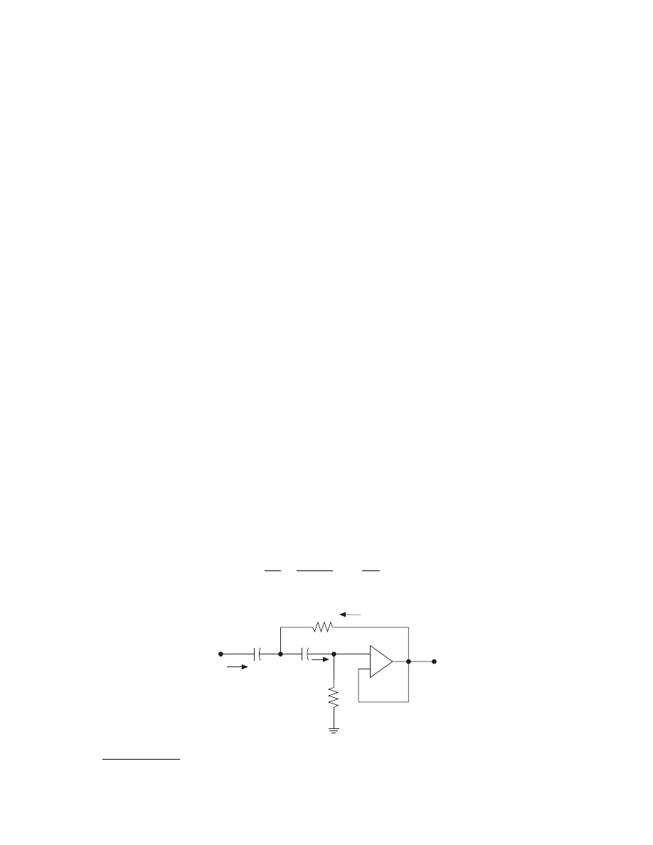
Once KCL has been written for the nodes of a circuit, the equations can be rewritten by substituting into
the equations the voltage-current relationships of the individual components. If a circuit is resistive, the resulting
equations will be algebraic. If capacitors or inductors are included in the circuit, the substitution will produce
a differential equation. For example, writing KCL at the node for
v
3
produces
i
2
+
i
1
–
i
3
= 0
and
FIGURE 3.2
Example of a circuit containing energy storage elements.
i
km
t
( )
å
0
=
C
dv
dt
v
v
R
C
dv
dt
1
1
4
3
2
2
2
0
+
-
-
=
R
1
C
2
R
2
i
1
+
–
v
2
+
+
–
–
v
1
i
2
C
1
v
3
v
in
v
4
i
3

© 2000 by CRC Press LLC
KCL for the node between C
2
and R
1
can be written to eliminate variables and lead to a solution describing
the capacitor voltages. The capacitor voltages, together with the applied voltage source, determine the remaining
voltages and currents in the circuit. Nodal analysis (see Section 3.2) treats the systematic modeling and analysis
of a circuit under the influence of its sources and energy storage elements.
Kirchhoff’s Current Law in the Complex Domain
Kirchhoff ’s current law is ordinarily stated in terms of the real (time-domain) currents flowing in a circuit,
because it actually describes physical quantities, at least in a macroscopic, statistical sense. It also applied,
however, to a variety of purely mathematical models that are commonly used to analyze circuits in the so-called
complex domain.
For example, if a linear circuit is in the sinusoidal steady state, all of the currents and voltages in the circuit
are sinusoidal. Thus, each voltage has the form
v(t) = A sin(
wt + f )
and each current has the form
i(t) = B sin(
wt + q)
where the positive coefficients A and B are called the magnitudes of the signals, and
f and q are the phase
angles of the signals. These mathematical models describe the physical behavior of electrical quantities, and
instrumentation, such as an oscilloscope, can display the actual waveforms represented by the mathematical
model. Although methods exist for manipulating the models of circuits to obtain the magnitude and phase
coefficients that uniquely determine the waveform of each voltage and current, the manipulations are cumber-
some and not easily extended to address other issues in circuit analysis.
Steinmetz [Smith and Dorf, 1992] found a way to exploit complex algebra to create an elegant framework
for representing signals and analyzing circuits when they are in the steady state. In this approach, a model is
developed in which each physical sign is replaced by a “complex” mathematical signal. This complex signal in
polar, or exponential, form is represented as
v
c
(t) = Ae
( j
wt + f )
The algebra of complex exponential signals allows us to write this as
v
c
(t) = Ae
j
f
e
j
wt
and Euler’s identity gives the equivalent rectangular form:
v
c
(t) = A[cos(
wt + f ) + j sin(wt + f )]
So we see that a physical signal is either the real (cosine) or the imaginary (sine) component of an abstract,
complex mathematical signal. The additional mathematics required for treatment of complex numbers allows
us to associate a phasor, or complex amplitude, with a sinusoidal signal. The time-invariant phasor associated
with v(t) is the quantity
V
c
= Ae
j
f
Notice that the phasor v
c
is an algebraic constant and that in incorporates the parameters A and
f of the
corresponding time-domain sinusoidal signal.
Phasors can be thought of as being vectors in a two-dimensional plane. If the vector is allowed to rotate
about the origin in the counterclockwise direction with frequency
w, the projection of its tip onto the horizontal

© 2000 by CRC Press LLC
(real) axis defines the time-domain signal corresponding to the real part of v
c
(t), i.e., A cos[
wt + f], and its
projection onto the vertical (imaginary) axis defines the time-domain signal corresponding to the imaginary
part of v
c
(t), i.e., A sin[
wt + f].
The composite signal v
c
(t) is a mathematical entity; it cannot be seen with an oscilloscope. Its value lies in
the fact that when a circuit is in the steady state, its voltages and currents are uniquely determined by their
corresponding phasors, and these in turn satisfy Kirchhoff ’s voltage and current laws! Thus, we are able to write
where I
km
is the phasor of i
km
(t), the sinusoidal current in branch k attached to node m. An equation of this
form can be written at each node of the circuit. For example, at node b in
KCL would have the form
I
1
– I
2
+ I
3
= 0
Consequently, a set of linear, algebraic equations describe the phasors of the currents and voltages in a circuit
in the sinusoidal steady state, i.e., the notion of time is suppressed (see Section 3.2). The solution of the set of
equations yields the phasor of each voltage and current in the circuit, from which the actual time-domain
expressions can be extracted.
It can also be shown that KCL can be extended to apply to the Fourier transforms and the Laplace transforms
of the currents in a circuit. Thus, a single relationship between the currents at the nodes of a circuit applies to
all of the known mathematical representations of the currents [Ciletti, 1988].
Kirchhoff’s Voltage Law
Kirchhoff ’s voltage law (KVL) describes a relationship among the voltages measured across the branches in any
closed, connected path in a circuit. Each branch in a circuit is connected to two nodes. For the purpose of
applying KVL, a path has an orientation in the sense that in “walking” along the path one would enter one of
the nodes and exit the other. This establishes a direction for determining the voltage across a branch in the
path: the voltage is the difference between the potential of the node entered and the potential of the node at
which the path exits. Alternatively, the voltage drop along a branch is the difference of the node voltage at the
entered node and the node voltage at the exit node. For example, if a path includes a branch between node “a”
and node “b”, the voltage drop measured along the path in the direction from node “a” to node “b” is denoted
by v
ab
and is given by v
ab
= v
a
– v
b
. Given v
ab
, branch voltage along the path in the direction from node “b” to
node “a” is v
ba
= v
b
– v
a
= –v
ab
.
Kirchhoff ’s voltage law, like Kirchhoff ’s current law, is true at any time. KVL can also be stated in terms of
voltage rises instead of voltage drops.
KVL can be expressed mathematically as “the algebraic sum of the voltages drops around any closed path of
a circuit at any instant of time is zero.” This statement can also be cast as an equation:
where v
km
(t) is the instantaneous voltage drop measured across branch k of path m. By convention, the voltage
drop is taken in the direction of the edge sequence that forms the path.
The edge sequence {e
1
, e
2
, e
3
, e
4
, e
6
, e
7
} forms a closed path in Fig. 3.1. The sum of the voltage drops taken
around the path must satisfy KVL:
v
ab
(t) + v
bc
(t) + v
cd
(t) + v
de
(t) + v
ef
(t) + v
fa
(t) = 0
Since v
af
(t) = –v
fa
(t), we can also write
I
km
å
0
=
v
km
t
( )
å
0
=

© 2000 by CRC Press LLC
v
af
(t) = v
ab
(t) + v
bc
(t) + v
cd
(t) + v
de
(t) + v
ef
(t)
Had we chosen the path corresponding to the edge sequence {e
1
, e
5
, e
6
, e
7
} for the path, we would have obtained
v
af
(t) = v
ab
(t) + v
be
(t) + v
ef
(t)
This demonstrates how KCL can be used to determine the voltage between a pair of nodes. It also reveals the
fact that the voltage between a pair of nodes is independent of the path between the nodes on which the voltages
are measured.
Kirchhoff’s Voltage Law in the Complex Domain
Kirchhoff ’s voltage law also applies to the phasors of the voltages in a circuit in steady state and to the Fourier
transforms and Laplace transforms of the voltages in a circuit.
Importance of KVL and KCL
Kirchhoff ’s current law is used extensively in nodal analysis because it is amenable to computer-based imple-
mentation and supports a systematic approach to circuit analysis. Nodal analysis leads to a set of algebraic
equations in which the variables are the voltages at the nodes of the circuit. This formulation is popular in
CAD programs because the variables correspond directly to physical quantities that can be measured easily.
Kirchhoff ’s voltage law can be used to completely analyze a circuit, but it is seldom used in large-scale circuit
simulation programs. The basic reason is that the currents that correspond to a loop of a circuit do not
necessarily correspond to the currents in the individual branches of the circuit. Nonetheless, KVL is frequently
used to troubleshoot a circuit by measuring voltage drops across selected components.
Defining Terms
Branch:
A symbol representing a path for current through a component in an electrical circuit.
Branch current:
The current in a branch of a circuit.
Branch voltage:
The voltage across a branch of a circuit.
Independent source:
A voltage (current) source whose voltage (current) does not depend on any other voltage
or current in the circuit.
Node:
A symbol representing a physical connection between two electrical components in a circuit.
Node voltage:
The voltage between a node and a reference node (usually ground).
Related Topic
3.6 Graph Theory
References
M.D. Ciletti, Introduction to Circuit Analysis and Design, New York: Holt, Rinehart and Winston, 1988.
R.H. Smith and R.C. Dorf, Circuits, Devices and Systems, New York: Wiley, 1992.
Further Information
Kirchhoff ’s laws form the foundation of modern computer software for analyzing electrical circuits. The
interested reader might consider the use of determining the minimum number of algebraic equations that fully
characterizes the circuit. It is determined by KCL, KVL, or some mixture of the two?
© 2000 by CRC Press LLC
3.2 Node and Mesh Analysis
J. David Irwin
In this section Kirchhoff ’s current law (KCL) and Kirchhoff ’s voltage law (KVL) will be used to determine
currents and voltages throughout a network. For simplicity, we will first illustrate the basic principles of both
node analysis and mesh analysis using only dc circuits. Once the fundamental concepts have been explained
and illustrated, we will demonstrate the generality of both analysis techniques through an ac circuit example.
Node Analysis
In a node analysis, the node voltages are the variables in a circuit,
and KCL is the vehicle used to determine them. One node in the
network is selected as a reference node, and then all other node
voltages are defined with respect to that particular node. This refer-
ence node is typically referred to as ground using the symbol ( ),
indicating that it is at ground-zero potential.
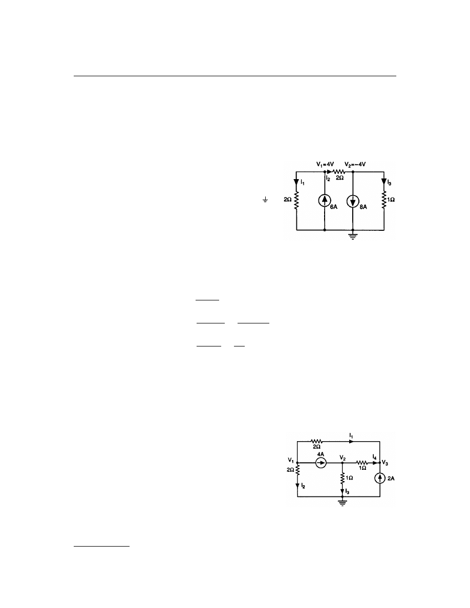
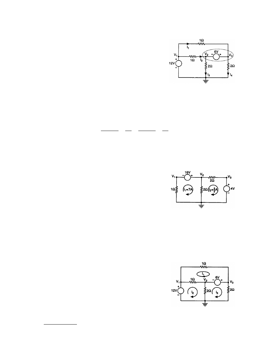
Consider the network shown in
. The network has three
nodes, and the nodes at the bottom of the circuit has been selected
as the reference node. Therefore the two remaining nodes, labeled
V
1
and V
2
, are measured with respect to this reference node.
Suppose that the node voltages V
1
and V
2
have somehow been
determined, i.e., V
1
= 4 V and v
2
= –4 V. Once these node voltages
are known, Ohm’s law can be used to find all branch currents. For example,
Note that KCL is satisfied at every node, i.e.,
I
1
– 6 + I
2
= 0
–I
2
+ 8 + I
3
= 0
–I
1
+ 6 – 8 – I
3
= 0
Therefore, as a general rule, if the node voltages are known, all
branch currents in the network can be immediately determined.
In order to determine the node voltages in a network, we apply
KCL to every node in the network except the reference node. There-
fore, given an N-node circuit, we employ N – 1 linearly independent
simultaneous equations to determine the N – 1 unknown node volt-
ages. Graph theory, which is covered in Section 3.6, can be used to
prove that exactly N – 1 linearly independent KCL equations are
required to find the N – 1 unknown node voltages in a network.
Let us now demonstrate the use of KCL in determining the node
voltages in a network. For the network shown in
, the bottom
FIGURE 3.3
A three-node network.
I
V
I
V
V
I
V
1
1
2
1
2
3
2
0
2
2
2
4
4
2
4
0
1
4
1
4
=
-
=
=
-
=
- -
=
=
-
=
-
= -
A
A
A
(
)
FIGURE 3.4
A four-node network.
© 2000 by CRC Press LLC
node is selected as the reference and the three remaining nodes, labeled V
1
, V
2
, and V
3
, are measured with
respect to that node. All unknown branch currents are also labeled. The KCL equations for the three nonref-
erence nodes are
I
1
+ 4 + I
2
= 0
– 4 + I
3
+ I
4
= 0
–I
1
– I
4
– 2 = 0
Using Ohm’s law these equations can be expressed as
Solving these equations, using any convenient method, yields
V
1
= –8/3 V, V
2
= 10/3 V, and V
3
= 8/3 V. Applying Ohm’s law
we find that the branch currents are I
1
= –16/6 A, I
2
= –8/6 A,
I
3
= 20/6 A, and I
4
= 4/6 A. A quick check indicates that KCL
is satisfied at every node.
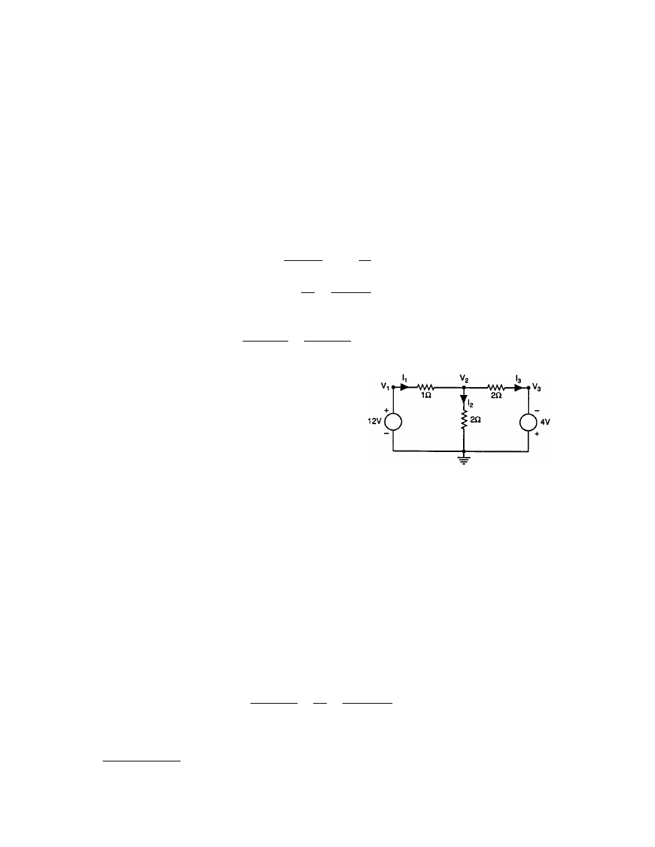
The circuits examined thus far have contained only current
sources and resistors. In order to expand our capabilities, we
next examine a circuit containing voltage sources. The circuit
shown in
has three nonreference nodes labeled V
1
, V
2
,
and V
3
. However, we do not have three unknown node volt-
ages. Since known voltage sources exist between the reference
node and nodes V
1
and V
3
, these two node voltages are known, i.e., V
1
= 12 V and V
3
= –4 V. Therefore, we
have only one unknown node voltage, V
2
. The equations for this network are then
V
1
= 12
V
3
= – 4
and
–I
1
+ I
2
+ I
3
= 0
The KCL equation for node V
2
written using Ohm’s law is
Solving this equation yields V
2
= 5 V, I
1
= 7 A, I
2
= 5/2 A, and I
3
= 9/2 A. Therefore, KCL is satisfied at every node.
V
V
V
V
V
V
1
3
1
2
2
3
2
4
2
0
4
1
1
0
-
+
+
=
-
+
+
-
=
-
-
-
-
-
=
(
)
(
)
V
V
V
V
1
3
2
3
2
1
2
0
FIGURE 3.5
A four-node network containing
voltage sources.
-
-
+
+
- -
=
(
)
(
)
12
1
2
4
2
0
2
2
2
V
V
V
© 2000 by CRC Press LLC
Thus, the presence of a voltage source in the network actually
simplifies a node analysis. In an attempt to generalize this idea,
consider the network in
. Note that in this case V
1
= 12 V and
the difference between node voltages V
3
and V
2
is constrained to be
6 V. Hence, two of the three equations needed to solve for the node
voltages in the network are
V
1
= 12
V
3
– V
2
= 6
To obtain the third required equation, we form what is called a
supernode, indicated by the dotted enclosure in the network. Just as KCL must be satisfied at any node in the
network, it must be satisfied at the supernode as well. Therefore, summing all the currents leaving the supernode
yields the equation
The three equations yield the node voltages V
1
= 12 V, V
2
= 5 V, and V
3
= 11 V, and therefore I
1
= 1 A, I
2
= 7
A, I
3
= 5/2 A, and I
4
= 11/2 A.
Mesh Analysis
In a mesh analysis the mesh currents in the network are the variables
and KVL is the mechanism used to determine them. Once all the mesh
currents have been determined, Ohm’s law will yield the voltages
anywhere in e circuit. If the network contains N independent meshes,
then graph theory can be used to prove that N independent linear
simultaneous equations will be required to determine the N mesh
currents.
The network shown in
has two independent meshes. They
are labeled I
1
and I
2
, as shown. If the mesh currents are known to be
I
1
= 7 A and I
2
= 5/2 A, then all voltages in the network can be
calculated. For example, the voltage V
1
, i.e., the voltage across the 1-
W
resistor, is V
1
= –I
1
R = –(7)(1) = –7 V. Likewise V = (I
1
– I
2
)R = (7 –5/2)(2) = 9 V. Furthermore, we can check
our analysis by showing that KVL is satisfied around every mesh. Starting at the lower left-hand corner and
applying KVL to the left-hand mesh we obtain
–(7)(1) + 16 – (7 – 5/2)(2) = 0
where we have assumed that increases in energy level are positive and
decreases in energy level are negative.
Consider now the network in
. Once again, if we assume that
an increase in energy level is positive and a decrease in energy level is
negative, the three KVL equations for the three meshes defined are
–I
1
(1) – 6 – (I
1
– I
2
)(1) = 0
+12 – (I
2
– I
1
)(1) – (I
2
– I
3
)(2) = 0
–(I
3
– I
2
)(2) + 6 – I
3
(2) = 0
FIGURE 3.6
A four-node network used to
illustrate a supernode.
V
V
V
V
V
V
2
1
2
3
1
3
1
2
1
2
0
-
+
+
-
+
=
FIGURE 3.7
A network containing two
independent meshes.
FIGURE 3.8
A three-mesh network.
© 2000 by CRC Press LLC
These equations can be written as
2I
1
– I
2
= –6
–I
12
+ 3I
2
– 2I
3
= 12
– 2I
2
+ 4I
3
= 6
Solving these equations using any convenient method yields I1 = 1 A,
I
2
= 8 A, and I
3
= 11/2 A. Any voltage in the network can now be easily
calculated, e.g., V
2
= (I
2
– I
3
)(2) = 5 V and V
3
= I
3
(2) = 11 V.
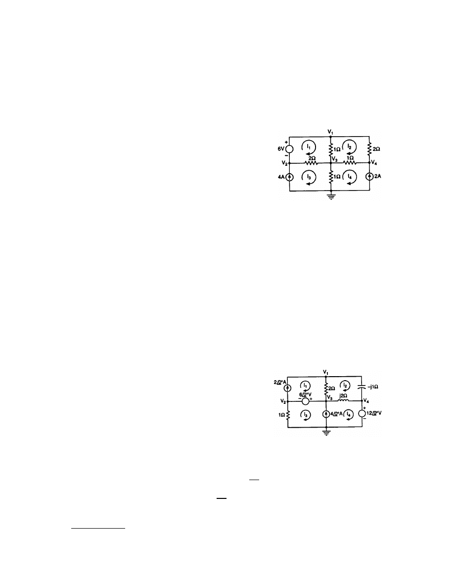
Just as in the node analysis discussion, we now expand our capa-
bilities by considering circuits which contain current sources. In this
case, we will show that for mesh analysis, the presence of current
sources makes the solution easier.
The network in
has four meshes which are labeled I
1
, I
2
, I
3
,
and I
4
. However, since two of these currents, i.e., I
3
and I
4
, pass directly
through a current source, two of the four linearly independent equa-
tions required to solve the network are
I
3
= 4
I
4
= –2
The two remaining KVL equations for the meshes defined by I
1
and I
2
are
+6 – (I
1
– I
2
)(1) – (I
1
– I
3
)(2) = 0
–(I
2
– I
1
)(1) – I
2
(2) – (I
2
– I
4
)(1) = 0
Solving these equations for I
1
and I
2
yields I
1
= 54/11 A and I
2
= 8/11 A. A quick check will show that KCL is
satisfied at every node. Furthermore, we can calculate any node voltage in the network. For example, V
3
= (I
3
–
I
4
)(1) = 6 V and V
1
= V
3
+ (I
1
– I
2
)(1) = 112/11 V.
Summary
Both node analysis and mesh analysis have been presented and dis-
cussed. Although the methods have been presented within the frame-
work of dc circuits with only independent sources, the techniques
are applicable to ac analysis and circuits containing dependent
sources.
To illustrate the applicability of the two techniques to ac circuit
analysis, consider the network in
. All voltages and currents
are phasors and the impedance of each passive element is known.
In the node analysis case, the voltage V
4
is known and the voltage
between V
2
and V
3
is constrained. Therefore, two of the four required
equations are
V
4
= 12
/
0
°
V
2
+ 6
/
0
° = V
3
KCL for the node labeled V
1
and the supernode containing the nodes labeled V
2
and V
3
is
FIGURE 3.9
A four-mesh network con-
taining current sources.
FIGURE 3.10
A network containing five
nodes and four meshes.

© 2000 by CRC Press LLC
Solving these equations yields the remaining unknown node voltages.
V
1
= 11.9 – j0.88 = 11.93
/
– 4.22
° V
V
2
= 3.66 – j1.07 = 3.91
/
–16.34
° V
V
3
= 9.66 – j1.07 = 9.72
/
–6.34
° V
In the mesh analysis case, the currents I
1
and I
3
are constrained to be
I
1
= 2
/
0
°
I
4
– I
3
= – 4
/
0
°
The two remaining KVL equations are obtained from the mesh defined by mesh current I
2
and the loop which
encompasses the meshes defined by mesh currents I
3
and I
4
.
–2(I
2
– I
1
) – (–j1)I
2
– j2(I
2
– I4) = 0
–(1I
3
+ 6
/
0
° – j2(I
4
– I
2
) – 12
/
0
° = 0
Solving these equations yields the remaining unknown mesh currents
I
2
= 0.88
/
–6.34
° A
I
3
= 3.91
/
163.66
° A
I
4
= 1.13
/
72.35
° A
As a quick check we can use these currents to compute the node voltages. For example, if we calculate
V
2
= –1(I
3
)
and
V
1
= –j1(I
2
) + 12
/
0
°
we obtain the answers computed earlier.
As a final point, because both node and mesh analysis will yield all currents and voltages in a network, which
technique should be used? The answer to this question depends upon the network to be analyzed. If the network
contains more voltage sources than current sources, node analysis might be the easier technique. If, however,
the network contains more current sources than voltage sources, mesh analysis may be the easiest approach.
V
V
V
V
V
V
V
V
V
1
3
1
4
2
3
1
3
4
2
1
2 0
1
2 0
2
2
4 0
0
-
+
-
-
=
°
+
° +
-
+
-
=
° =
j
j
/
/
/
© 2000 by CRC Press LLC
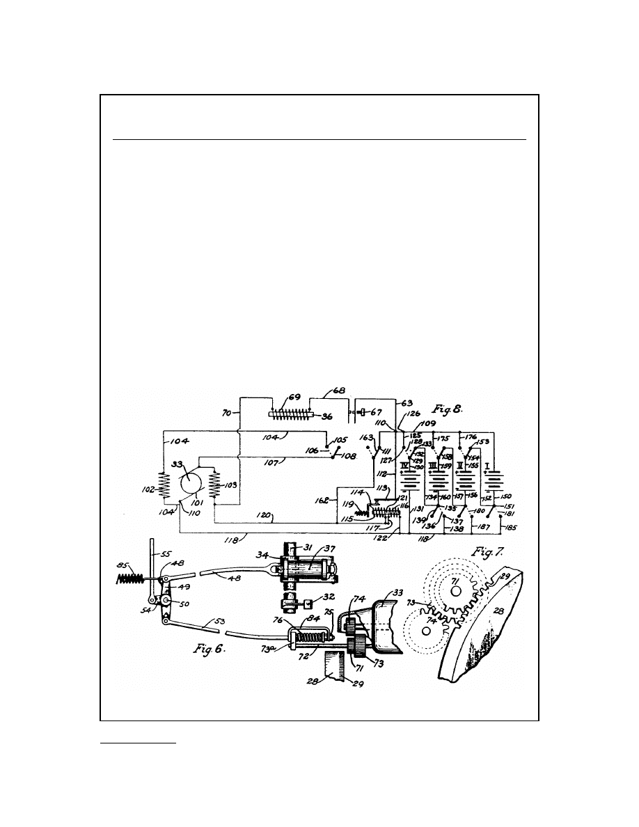
E
NGINE
-S
TARTING
D
EVICE
Charles F. Kettering
Patented August 17, 1915
#1,150,523
arly automobiles were all started with a crank, or arm-strong starters, as they were known. This
backbreaking process was difficult for everyone, especially women. And it was dangerous. Backfires
often resulted in broken wrists. Worse yet, if accidentally left in gear, the car could advance upon
the person cranking. Numerous deaths and injuries were reported.
In 1910, Henry Leland, Cadillac Motors president, commissioned Charles Kettering and his Dayton
Engineering Laboratories Company to develop an electric self-starter to replace the crank. Kettering had
to overcome two large problems: (1) making a motor small enough to fit in a car yet powerful enough
to crank the engine, and (2) finding a battery more powerful than any yet in existence. Electric Storage
Battery of Philadelphia supplied an experimental 65-lb battery and Delco unveiled a working prototype
electric “self-starter” system installed in a 1912 Cadillac on February 17, 1911. Leland immediately ordered
12,000 units for Cadillac. Within a few years, almost all new cars were equipped with electric starters.
(Copyright © 1995, DewRay Products, Inc. Used with permission.)
E
© 2000 by CRC Press LLC
Defining Terms
ac:
An abbreviation for alternating current.
dc: An abbreviation for direct current.
Kirchhoff ’s current law (KCL):
This law states that the algebraic sum of the currents either entering or leaving
a node must be zero. Alternatively, the law states that the sum of the currents entering a node must be
equal to the sum of the currents leaving that node.
Kirchhoff ’s voltage law (KVL):
This law states that the algebraic sum of the voltages around any loop is zero.
A loop is any closed path through the circuit in which no node is encountered more than once.
Mesh analysis:
A circuit analysis technique in which KVL is used to determine the mesh currents in a network.
A mesh is a loop that does not contain any loops within it.
Node analysis:
A circuit analysis technique in which KCL is used to determine the node voltages in a network.
Ohm’s law:
A fundamental law which states that the voltage across a resistance is directly proportional to the
current flowing through it.
Reference node:
One node in a network that is selected to be a common point, and all other node voltages
are measured with respect to that point.
Supernode:
A cluster of node, interconnected with voltage sources, such that the voltage between any two
nodes in the group is known.
Related Topics
3.1 Voltage and Current Laws • 3.6 Graph Theory
Reference
J.D. Irwin, Basic Engineering Circuit Analysis, 5th ed., Upper Saddle River, N.J.: Prentice-Hall, 1996.
3.3 Network Theorems
Allan D. Kraus
Linearity and Superposition
Linearity
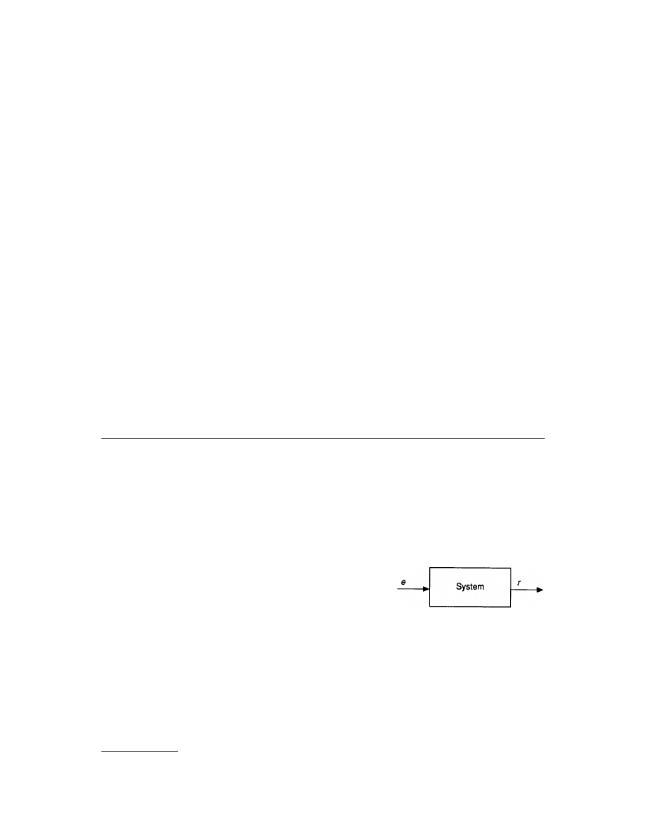
Consider a system (which may consist of a single network element) represented by a block, as shown in
and observe that the system has an input designated by e (for excitation) and an output designated by r (for
response). The system is considered to be linear if it satisfies the homogeneity and superposition conditions.
The homogeneity condition: If an arbitrary input to the system, e,
causes a response, r, then if ce is the input, the output is cr where c is
some arbitrary constant.
The superposition condition: If the input to the system, e
1
, causes a
response, r
1
, and if an input to the system, e
2
, causes a response, r
2
,
then a response, r
1
+ r
2
, will occur when the input is e
1
+ e
2
.
If neither the homogeneity condition nor the superposition condi-
tion is satisfied, the system is said to be nonlinear.
The Superposition Theorem
While both the homogeneity and superposition conditions are necessary for linearity, the superposition con-
dition, in itself, provides the basis for the superposition theorem:
If cause and effect are linearly related, the total effect due to several causes acting simultaneously is equal to
the sum of the individual effects due to each of the causes acting one at a time.
FIGURE 3.11
A simple system.
© 2000 by CRC Press LLC
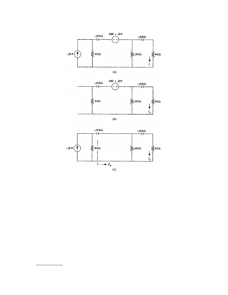
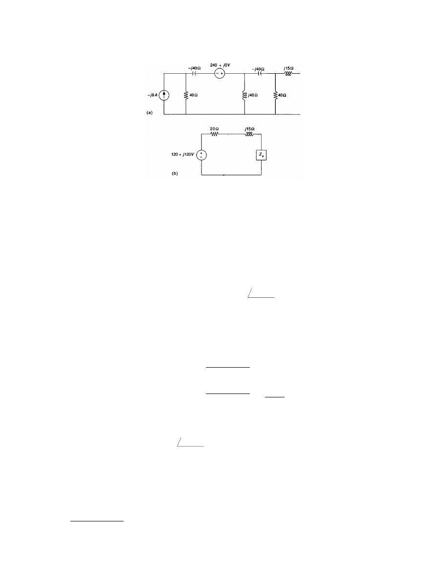
Example 3.1. Consider the network driven by a current source at the left and a voltage source at the top, as
shown in
. The current phasor indicated by
^
I is to be determined. According to the superposition
theorem, the current
^
I will be the sum of the two current components
^
I
V
due to the voltage source acting alone
as shown in
and
^
I
C
due to the current source acting alone shown in
Figures 3.12(b) and (c) follow from the methods of removing the effects of independent voltage and current
sources. Voltage sources are nulled in a network by replacing them with short circuits and current sources are
nulled in a network by replacing them with open circuits.
The networks displayed in Figs. 3.12(b) and (c) are simple ladder networks in the phasor domain, and the
strategy is to first determine the equivalent impedances presented to the voltage and current sources. In
Fig. 3.12(b), the group of three impedances to the right of the voltage source are in series-parallel and possess
an impedance of
FIGURE 3.12
(a) A network to be solved by using superposition; (b) the network with the current source nulled; and
(c) the network with the voltage source nulled.
ˆ
ˆ
ˆ
I
I
I
V
C
=
+

© 2000 by CRC Press LLC
and the total impedance presented to the voltage source is
Z = Z
P
+ 40 – j40 = 40 + j40 + 40 – j40 = 80
W
Then
^
I
1
, the current leaving the voltage source, is
and by a current division
In Fig. 3.12(b), the current source delivers current to the 40-
W resistor and to an impedance consisting of
the capacitor and Z
p
. Call this impedance Z
a
so that
Z
a
= –j40 + Z
P
= –j40 + 40 + j40 = 40
W
Then, two current divisions give
^
I
C
The current
^
I in the circuit of Fig. 3.12(a) is
^
I =
^
I
V
+
^
I
C
= 0 + j3 + (3 + j0) = 3 + j3 A
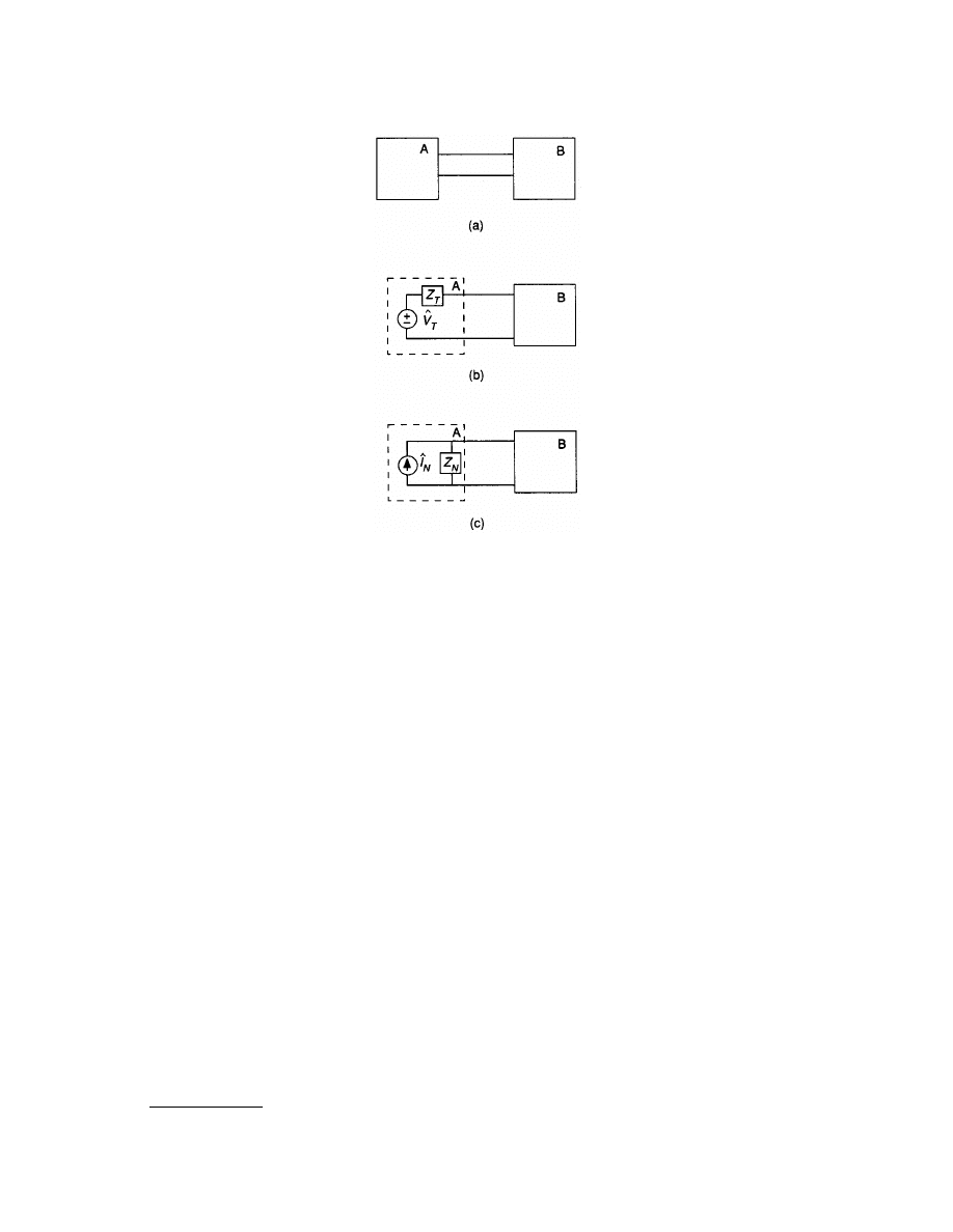
The Network Theorems of Thévenin and Norton
If interest is to be focused on the voltages and across the currents through a small portion of a network such
as network B in
, it is convenient to replace network A, which is complicated and of little interest,
by a simple equivalent. The simple equivalent may contain a single, equivalent, voltage source in series with
an equivalent impedance in series as displayed in
. In this case, the equivalent is called a Thévenin
equivalent. Alternatively, the simple equivalent may consist of an equivalent current source in parallel with an
equivalent impedance. This equivalent, shown in
, is called a Norton equivalent. Observe that as
long as Z
T
(subscript T for Thévenin) is equal to Z
N
(subscript N for Norton), the two equivalents may be
obtained from one another by a simple source transformation.
Conditions of Application
The Thévenin and Norton network equivalents are only valid at the terminals of network A in Fig. 3.13(a) and
they do not extend to its interior. In addition, there are certain restrictions on networks A and B. Network A
may contain only linear elements but may contain both independent and dependent sources. Network B, on
the other hand, is not restricted to linear elements; it may contain nonlinear or time-varying elements and may
Z
j
j
j
j
j
P
=
-
+
-
=
+
(
)(
)
40 40 40
40 40 40
40 40
W
ˆI
j
j
1
240 0
80
3
0
=
+
=
+
A
ˆ
(
)
(
)
I
j
j
j
j
j
j
j
V
=
-
+
é
ë
ê
ê
ù
û
ú
ú
+
=
+
=
+
40
40 40 40
3
0
3
0
0
3 A
ˆ
(
)
(
)
I
j
j
j
j
j
j
j
C
=
+
é
ë
ê
ê
ù
û
ú
ú
-
+
é
ë
ê
ê
ù
û
ú
ú
-
=
-
=
+
40
40 40
40
40 40 40
0
6
2
0
6
3
0 A
© 2000 by CRC Press LLC
also contain both independent and dependent sources. Together, there can be no controlled source coupling
or magnetic coupling between networks A and B.
The Thévenin Theorem
The statement of the Thévenin theorem is based on Fig. 3.13(b):
Insofar as a load which has no magnetic or controlled source coupling to a one-port is concerned, a network
containing linear elements and both independent and controlled sources may be replaced by an ideal voltage
source of strength,
^
V
T
, and an equivalent impedance Z
T
, in series with the source. The value of
^
V
T
is the
open-circuit voltage,
^
V
OC
, appearing across the terminals of the network and Z
T
is the driving point imped-
ance at the terminals of the network, obtained with all independent sources set equal to zero.
The Norton Theorem
The Norton theorem involves a current source equivalent. The statement of the Norton theorem is based on
Fig. 3.13(c):
Insofar as a load which has no magnetic or controlled source coupling to a one-port is concerned, the network
containing linear elements and both independent and controlled sources may be replaced by an ideal current
source of strength,
^
I
N
, and an equivalent impedance, Z
N
, in parallel with the source. The value of
^
I
N
is the
short-circuit current,
^
I
SC
, which results when the terminals of the network are shorted and Z
N
is the driving
point impedance at the terminals when all independent sources are set equal to zero.
The Equivalent Impedance, Z
T
= Z
N
Three methods are available for the determination of Z
T
. All of them are applicable at the analyst’s discretion.
When controlled sources are present, however, the first method cannot be used.
The first method involves the direct calculation of Z
eq
= Z
T
= Z
N
by looking into the terminals of the network
after all independent sources have been nulled. Independent sources are nulled in a network by replacing all
independent voltage sources with a short circuit and all independent current sources with an open circuit.
FIGURE 3.13
(a) Two one-port networks; (b) the Thévenin equivalent for network a; and (c) the Norton equivalent for
network a.

© 2000 by CRC Press LLC
The second method, which may be used when controlled sources are present in the network, requires the
computation of both the Thévenin equivalent voltage (the open-circuit voltage at the terminals of the network)
and the Norton equivalent current (the current through the short-circuited terminals of the network). The
equivalent impedance is the ratio of these two quantities
The third method may also be used when controlled sources are present within the network. A test voltage
may be placed across the terminals with a resulting current calculated or measured. Alternatively, a test current
may be injected into the terminals with a resulting voltage determined. In either case, the equivalent resistance
can be obtained from the value of the ratio of the test voltage
^
V
o
to the resulting current
^
I
o
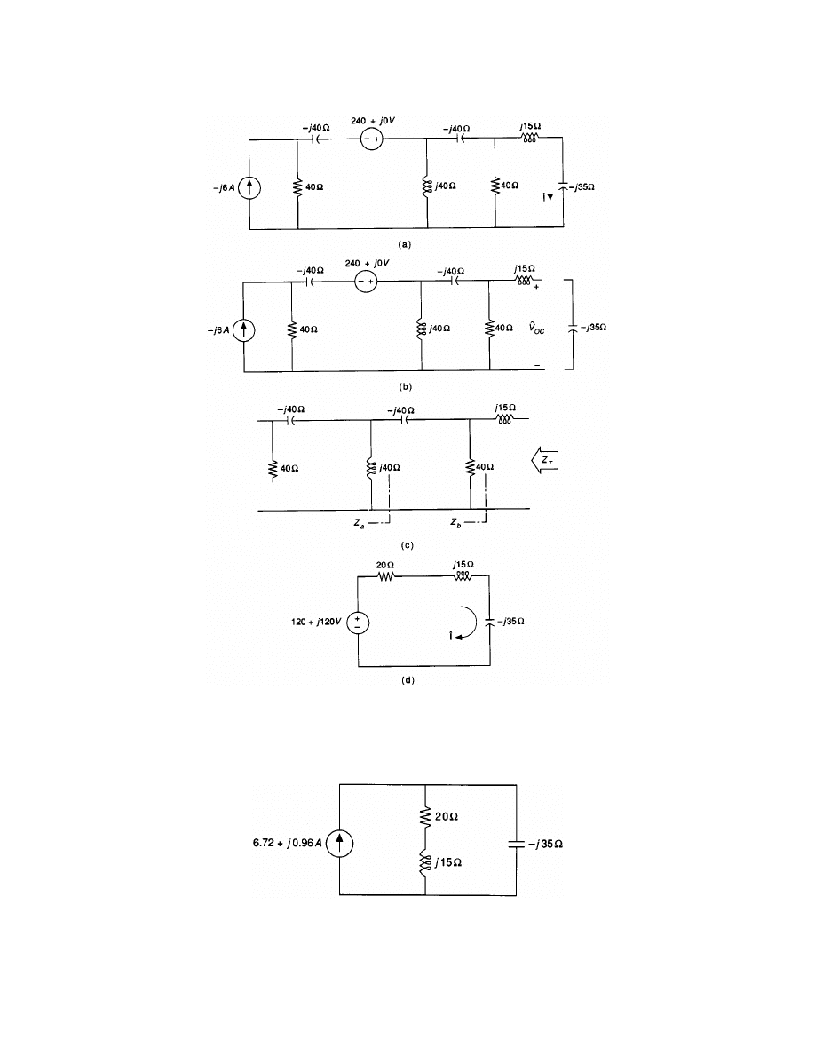
Example 3.2. The current through the capacitor with impedance –j35
W in
may be found using
Thévenin’s theorem. The first step is to remove the –j35-
W capacitor and consider it as the load. When this is
done, the network in
results.
The Thévenin equivalent voltage is the voltage across the 40–
W resistor. The current through the 40-W resistor
was found in Example 3.1 to be I = 3 + j3
W. Thus,
^
V
T
= 40(3 + j3) = 120 + j120 V
The Thévenin equivalent impedance may be found by looking into the terminals of the network in
. Observe that both sources in Fig. 3.14(a) have been nulled and that, for ease of computation,
impedances Z
a
and Z
b
have been placed on Fig. 3.14(c). Here,
and
Z
T
= Z
b
+ j15 = 20 + j15
W
Both the Thévenin equivalent voltage and impedance are shown in
, and when the load is attached,
as in Fig. 3.14(d), the current can be computed as
The Norton equivalent circuit is obtained via a simple voltage-to-current source transformation and is shown
. Here it is observed that a single current division gives
Z
Z
Z
V
I
V
I
T
N
eq
T
N
OC
SC
=
=
=
=
ˆ
ˆ
ˆ
ˆ
Z
V
I
T
o
o
=
ˆ
ˆ
Z
j
j
j
j
j
Z
a
b
=
-
+
-
=
+
=
+
=
(
)(
)
( )( )
40 40 40
40 40 40
40 40
40 40
40 40
20
W
W
ˆ
ˆ
I
V
j
j
j
j
j
T
=
+
-
=
+
-
=
+
20 15 35
120 120
20 20
0
6 A
ˆ
( . .
)
I
j
j
j
j
j
=
+
+
-
é
ë
ê
ê
ù
û
ú
ú
+
=
+
20 15
20 15 35
6 72 0 96 0 6 A
© 2000 by CRC Press LLC
FIGURE 3.14
(a) A network in the phasor domain; (b) the network with the load removed; (c) the network for the
computation of the Thévenin equivalent impedance; and (d) the Thévenin equivalent.
FIGURE 3.15
The Norton equivalent of Fig. 3.14(d).
© 2000 by CRC Press LLC
Tellegen’s Theorem
Tellegen’s theorem states:
In an arbitrarily lumped network subject to KVL and KCL constraints, with reference directions of the branch
currents and branch voltages associated with the KVL and KCL constraints, the product of all branch currents
and branch voltages must equal zero.
Tellegen’s theorem may be summarized by the equation
where the lower case letters v and j represent instantaneous values of the branch voltages and branch currents,
respectively, and where b is the total number of branches. A matrix representation employing the branch current
and branch voltage vectors also exists. Because V and J are column vectors
V · J = V
T
J = J
T
V
The prerequisite concerning the KVL and KCL constraints in the statement of Tellegen’s theorem is of crucial
importance.
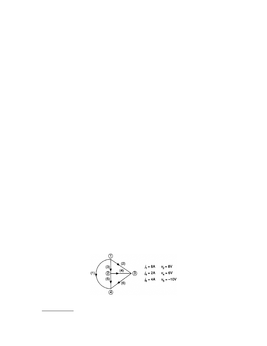
displays an oriented graph of a particular network in which there are six branches
labeled with numbers within parentheses and four nodes labeled by numbers within circles. Several known
branch currents and branch voltages are indicated. Because the type of elements or their values is not germane
to the construction of the graph, the other branch currents and branch voltages may be evaluated from repeated
applications of KCL and KVL. KCL may be used first at the various nodes.
node 3: j
2
= j
6
– j
4
= 4 – 2 = 2 A
node 1: j
3
= –j
1
– j
2
= –8 – 2 = –10 A
node 2: j
5
= j
3
– j
4
= –10 – 2 = –12 A
Then KVL gives
v
3
= v
2
– v
4
= 8 – 6 = 2 V
v
6
= v
5
– v
4
= –10 – 6 = –16 V
v
1
= v
2
+ v
6
= 8 – 16 = –8 V
FIGURE 3.16
An oriented graph of a particular network with some known branch currents and branch voltages.
v j
k k
k
b
=
=
å
0
1

© 2000 by CRC Press LLC
The transpose of the branch voltage and current vectors are
V
T
= [–8
8
2
6
–10
–16] V
and
J
T
= [8 2 –10 2 –12 4] V
The scalar product of V and J gives
–8(8) + 8(2) + 2(–10) + 6(2) + (–10)(–12) + (–16)(4) = –148 + 148 = 0
and Tellegen’s theorem is confirmed.
Maximum Power Transfer
The maximum power transfer theorem pertains to the connections of a load to the Thévenin equivalent of a
source network in such a manner as to transfer maximum power to the load. For a given network operating
at a prescribed voltage with a Thévenin equivalent impedance
Z
T
=
* Z
T
* q
T
the real power drawn by any load of impedance
Z
o
=
* Z
o
* q
o
is a function of just two variables,
* Z
o
* and q
o
. If the power is to be a maximum, there are three alternatives
to the selection of
* Z
o
* and q
o
:
(1) Both
* Z
o
* and q
o
are at the designer’s discretion and both are allowed to vary in any manner in order
to achieve the desired result. In this case, the load should be selected to be the complex conjugate of
the Thévenin equivalent impedance
Z
o
= Z *
T
(2) The angle,
q
o
, is fixed but the magnitude,
* Z
o
*, is allowed to vary. For example, the analyst may select
and fix
q
o
= 0
°. This requires that the load be resistive (Z is entirely real). In this case, the value of the
load resistance should be selected to be equal to the magnitude of the Thévenin equivalent impedance
R
o
=
* Z
T
*
(3) The magnitude of the load impedance,
* Z
o
*, can be fixed, but the impedance angle, q
o
, is allowed to
vary. In this case, the value of the load impedance angle should be
is identical to
with the exception of a load, Z
o
, substituted for the
capacitive load. The Thévenin equivalent is shown in
. The value of Z
o
to transfer maximum power
q
q
o
o
T
T
o
T
Z
Z
Z
Z
=
-
+
é
ë
ê
ê
ê
ù
û
ú
ú
ú
arcsin
sin
2
2
2
© 2000 by CRC Press LLC
is to be found if its elements are unrestricted, if it is to be a single resistor, or if the magnitude of Z
o
must be
20
W but its angle is adjustable.
For maximum power transfer to Z
o
when the elements of Z
o
are completely at the discretion of the network
designer, Z
o
must be the complex conjugate of Z
T
Z
o
= Z *
T
= 20 – j15
W
If Z
o
is to be a single resistor, R
o
, then the magnitude of Z
o
= R
o
must be equal to the magnitude of Z
T
. Here
Z
T
= 20 + j15 = 25 36.87
°
so that
R
o
=
* Z
o
* = 25 W
If the magnitude of Z
o
must be 20
W but the angle is adjustable, the required angle is calculated from
This makes Z
o
Z
o
= 20 –35.83
° = 16.22 – j11.71 W
The Reciprocity Theorem
The reciprocity theorem is a useful general theorem that applies to all linear, passive, and bilateral networks.
However, it applies only to cases where current and voltage are involved.
The ratio of a single excitation applied at one point to an observed response at another is invariant with
respect to an interchange of the points of excitation and observation.
FIGURE 3.17
(a) A network for which the load, Z
o
, is to be selected for maximum power transfer, and (b) the Thévenin
equivalent of the network.
q
q
o
o
T
o
T
T
Z
Z
Z
Z
=
-
+
é
ë
ê
ê
ù
û
ú
ú
=
-
+
°
é
ë
ê
ê
ù
û
ú
ú
=
-
= -
°
arcsin
sin
arcsin
( )( )
( )
( )
sin
.
arcsin(
.
)
.
/
2
2 20 25
20
25
36 87
0 585
35 83
2
2
2
2
* * *
*
* *
*
*
© 2000 by CRC Press LLC
The reciprocity principle also applies if the excitation is a current and the observed response is a voltage. It
will not apply, in general, for voltage–voltage and current–current situations, and, of course, it is not applicable
to network models of nonlinear devices.
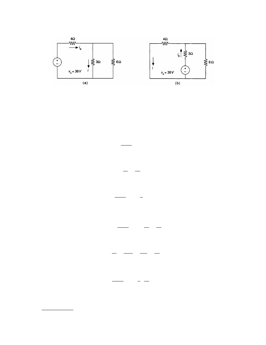
Example 3.5. It is easily shown that the positions of v
s
and i in
may be interchanged as in
without changing the value of the current i.
In Fig. 3.18(a), the resistance presented to the voltage source is
Then
and by current division
In Fig. 3.18(b), the resistance presented to the voltage source is
Then
and again, by current division
The network is reciprocal.
FIGURE 3.18
Two networks which can be used to illustrate the reciprocity principle.
R
=
+
+
=
+
=
4
3 6
3
6
4
2
6
( )
W
i
v
R
a
s
=
=
=
36
6
6 A
i
i
a
a
=
+
=
æ
è
ç
ö
ø
÷
=
6
6
3
2
3
6
4 A
R
=
+
+
=
+
=
3
6 4
6
4
3
12
5
27
5
( )
W
i
v
R
b
s
=
=
=
=
36
27 5
180
27
20
3
/
A
i
i
b
=
+
=
æ
è
ç
ö
ø
÷
=
6
4
6
3
5
20
3
4 A

© 2000 by CRC Press LLC
The Substitution and Compensation Theorems
The Substitution Theorem
Any branch in a network with branch voltage, v
k
, and branch current, i
k
, can be replaced by another branch
provided it also has branch voltage, v
k
, and branch current, i
k
.
The Compensation Theorem
In a linear network, if the impedance of a branch carrying a current
^
I is changed from Z to Z +
DZ, then the
corresponding change of any voltage or current elsewhere in the network will be due to a compensating voltage
source,
DZ
^
I, placed in series with Z +
DZ with polarity such that the source, DZ
^
I, is opposing the current
^
I.
Defining Terms
Linear network:
A network in which the parameters of resistance, inductance, and capacitance are constant
with respect to voltage or current or the rate of change of voltage or current and in which the voltage
or current of sources is either independent of or proportional to other voltages or currents, or their
derivatives.
Maximum power transfer theorem:
In any electrical network which carries direct or alternating current, the
maximum possible power transferred from one section to another occurs when the impedance of the
section acting as the load is the complex conjugate of the impedance of the section that acts as the source.
Here, both impedances are measured across the pair of terminals in which the power is transferred with
the other part of the network disconnected.
Norton theorem:
The voltage across an element that is connected to two terminals of a linear, bilateral network
is equal to the short-circuit current between these terminals in the absence of the element, divided by
the admittance of the network looking back from the terminals into the network, with all generators
replaced by their internal admittances.
Principle of superposition:
In a linear electrical network, the voltage or current in any element resulting
from several sources acting together is the sum of the voltages or currents from each source acting alone.
Reciprocity theorem:
In a network consisting of linear, passive impedances, the ratio of the voltage introduced
into any branch to the current in any other branch is equal in magnitude and phase to the ratio that
results if the positions of the voltage and current are interchanged.
Thévenin theorem:
The current flowing in any impedance connected to two terminals of a linear, bilateral
network containing generators is equal to the current flowing in the same impedance when it is connected
to a voltage generator whose voltage is the voltage at the open-circuited terminals in question and whose
series impedance is the impedance of the network looking back from the terminals into the network,
with all generators replaced by their internal impedances.
Related Topics
2.2 Ideal and Practical Sources • 3.4 Power and Energy
References
J. D. Irwin, Basic Engineering Circuit Analysis, 4th ed., New York: Macmillan, 1993.
A. D. Kraus, Circuit Analysis, St. Paul: West Publishing, 1991.
J. W. Nilsson, Electric Circuits, 5th ed., Reading, Mass.: Addison-Wesley, 1995.
Further Information
Three texts listed in the References have achieved widespread usage and contain more details on the material
contained in this section.
© 2000 by CRC Press LLC
3.4 Power and Energy
Norman Balabanian and Theodore A. Bickart
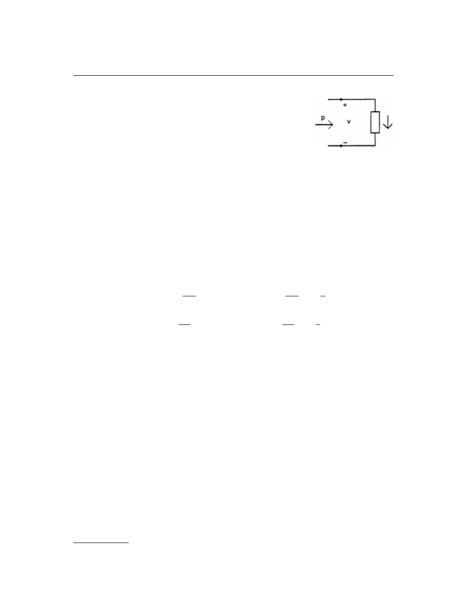
The concept of the voltage v between two points was introduced in Section 3.1
as the energy w expended per unit charge in moving the charge between the two
points. Coupled with the definition of current i as the time rate of charge motion
and that of power p as the time rate of change of energy, this leads to the following
fundamental relationship between the power delivered to a two-terminal elec-
trical component and the voltage and current of that component, with standard
references (meaning that the voltage reference plus is at the tail of the current
reference arrow) as shown in
p = vi (3.1)
Assuming that the voltage and current are in volts and amperes, respectively, the power is in watts. This
relationship applies to any two-terminal component or network, whether linear or nonlinear.
The power delivered to the basic linear resistive, inductive, and capacitive elements is obtained by inserting
the v-i relationships into this expression. Then, using the relationship between power and energy (power as
the time derivative of energy and energy, therefore, as the integral of power), the energy stored in the capacitor
and inductor is also obtained:
(3.2)
where the origin of time (t = 0) is chosen as the time when the capacitor voltage (respectively, the inductor
current) is zero.
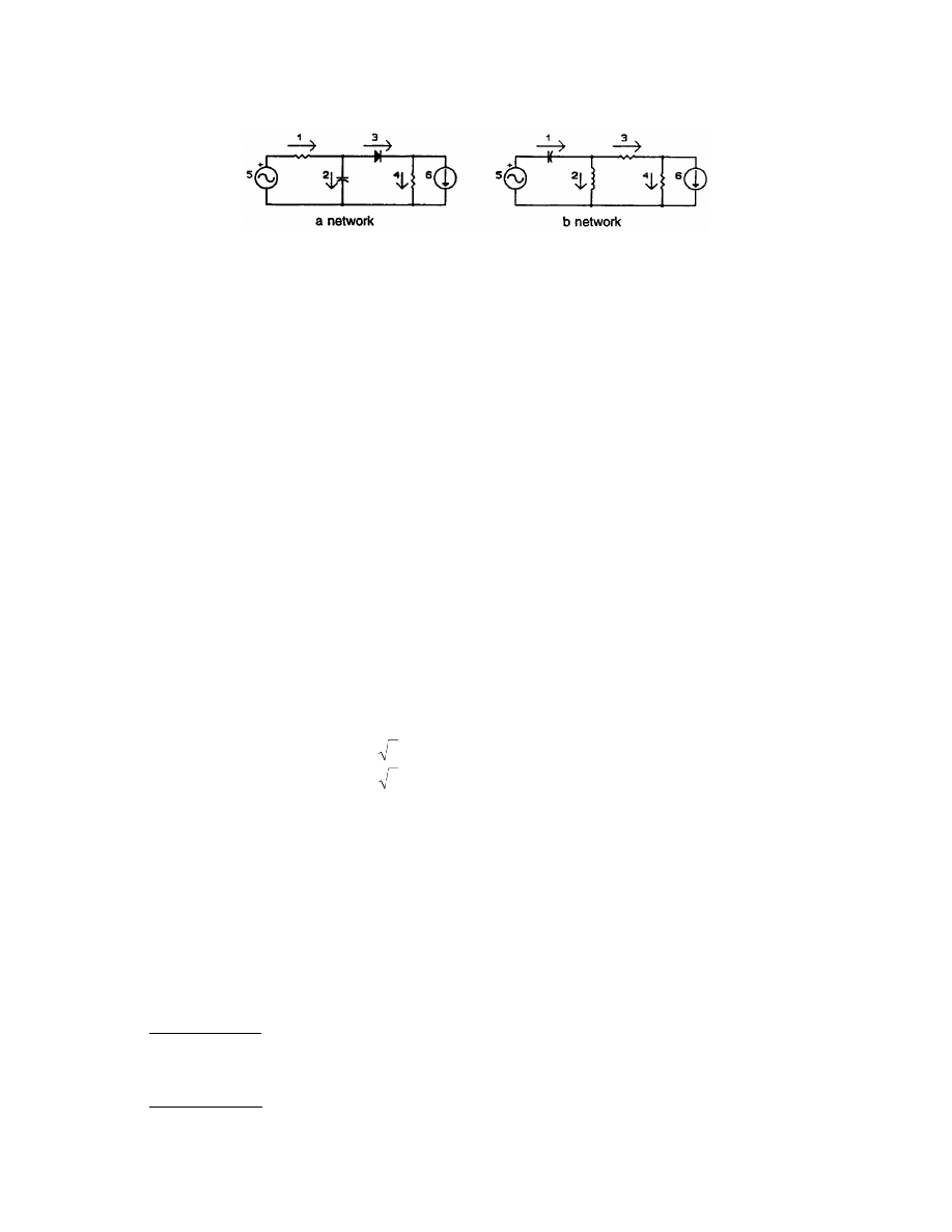
Tellegen’s Theorem
A result that has far-reaching consequences in electrical engineering is Tellegen’s theorem. It will be stated in
terms of the networks shown in
. These two are said to be topologically equivalent; that is, they are
represented by the same graph but the components that constitute the branches of the graph are not necessarily
the same in the two networks. they can even be nonlinear, as illustrated by the diode in one of the networks.
Assuming all branches have standard references, including the source branches, Tellegen’s theorem states that
(3.3)
In the second line, the variables are vectors and the prime stands for the transpose. The a and b subscripts refer
to the two networks.
FIGURE 3.19
Power deliv-
ered to a circuit.
p
v i
Ri
p
v i
Cv
dv
dt
w t Cv
dv
dt
dt Cv t
p
v i
Li
di
dt
w t Li
di
dt
dt Li t
R
R R
C
C C
C
C
C
C
C
t
C
L
L L
L
L
L
L
L
t
L
=
=
=
=
=
=
=
=
=
=
ò
ò
2
0
2
0
2
1
2
1
2
( ) ( )
( ) ( )
v i
bj aj
j
b a
all
·
å
=
¢ =
0
0
v i
© 2000 by CRC Press LLC
This is an amazing result. It can be easily proved with the use of Kirchhoff ’s two laws.
1
The products of v
and i are reminiscent of power as in Eq. (3.1). However, the product of the voltage of a branch in one network
and the current of its topologically corresponding branch (which may not even be the same type of component)
in another network does not constitute power in either branch. furthermore, the variables in one network might
be functions of time, while those of the other network might be steady-state phasors or Laplace transforms.
Nevertheless, some conclusions about power can be derived from Tellegen’s theorem. Since a network is
topologically equivalent to itself, the b network can be the same as the a network. In that case each vi product
in Eq. (3.3) represents the power delivered to the corresponding branch, including the sources. The equation
then says that if we add the power delivered to all the branches of a network, the result will be zero.
This result can be recast if the sources are separated from the other branches and one of the references of
each source (current reference for each v-source and voltage reference for each i-source) is reversed. Then the
vi product for each source, with new references, will enter Eq. (3.3) with a negative sign and will represent the
power supplied by this source. When these terms are transposed to the right side of the equation, their signs
are changed. The new equation will state in mathematical form that
In any electrical network, the sum of the power supplied by the sources is equal to the sum of the power
delivered to all the nonsource branches.
This is not very surprising since it is equivalent to the law of conservation of energy, a fundamental principle
of science.
AC Steady-State Power
Let us now consider the ac steady-state case, where all voltages and currents are sinusoidal. Thus, in the two-
terminal circuit of Fig. 3.19:
(3.4)
The capital V and I are phasors representing the voltage and current, and their magnitudes are the corresponding
rms values. The power delivered to the network at any instant of time is given by:
(3.5)
The last form is obtained by using trigonometric identities for the sum and difference of two angles. Whereas
both the voltage and the current are sinusoidal, the instantaneous power contains a constant term (independent
1
See, for example, N. Balabanian and T. A. Bickart, Linear Network Theory, Matrix Publishers, Chesterland, Ohio, 1981,
chap. 9.
FIGURE 3.20
Topologically equivalent networks.
v t
V
t
V
V e
i t
I
t
I
I e
j
j
( )
cos(
)
( )
cos(
)
=
+
«
=
=
+
«
=
2
2
* *
* *
* *
* *
w
a
w
b
a
b
p t
v t i t
V I
t
t
V I
V I
t
( )
( ) ( )
cos(
) cos(
)
cos(
)
cos(
)
=
=
+
+
=
-
[
]
+
+
+
[
]
2
2
* * * *
* * * *
* * * *
w
a
w
b
a
b
w
a
b
© 2000 by CRC Press LLC
of time) in addition to a sinusoidal term. Furthermore, the frequency of the sinusoidal term is twice that of
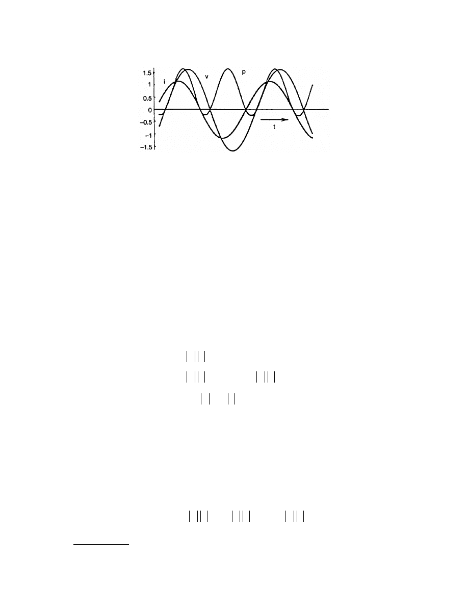
the voltage or current. Plots of v, i, and p are shown in
for specific values of
a and b. The power is
sometimes positive, sometimes negative. This means that power is sometimes delivered to the terminals and
sometimes extracted from them.
The energy which is transmitted into the network over some interval of time is found by integrating the
power over this interval. If the area under the positive part of the power curve were the same as the area under
the negative part, the net energy transmitted over one cycle would be zero. For the values of
a and b used in
the figure, however, the positive area is greater, so there is a net transmission of energy toward the network.
The energy flows back from the network to the source over part of the cycle, but on the average, more energy
flows toward the network than away from it.
In Terms of RMS Values and Phase Difference
Consider the question from another point of view. The preceding equation shows the power to consist of a
constant term and a sinusoid. The average value of a sinusoid is zero, so this term will contribute nothing to
the net energy transmitted. Only the constant term will contribute. This constant term is the average value of
the power, as can be seen either from the preceding figure or by integrating the preceding equation over one
cycle. Denoting the average power by P and letting
q = a – b, which is the angle of the network impedance,
the average power becomes:
(3.6)
The third line is obtained by breaking up the exponential in the previous line by the law of exponents. The
first factor between square brackets in this line is identified as the phasor voltage and the second factor as the
conjugate of the phasor current. The last line then follows. It expresses the average power in terms of the voltage
and current phasors and is sometimes more convenient to use.
Complex and Reactive Power
The average ac power is found to be the real part of a complex quantity VI*, labeled S, that in rectangular form is
(3.7)
FIGURE 3.21
Instantaneous voltage, current, and power.
P
V I
V I e V I e
V e I e
VI
j
j
j
j
=
=
(
)
=
[
]
=
(
)
(
)
[
]
=
( )
-
(
)
-
cos
Re Re
Re
Re *
q
q
a b
a
b
S
VI
V I e
V I
j V I
P
jQ
j
=
=
=
+
=
+
* cos sin
q
q
q
© 2000 by CRC Press LLC
where
(3.8)
We already know P to be the average power. Since it is the real part of some complex quantity, it would be
reasonable to call it the
. The complex quantity S of which P is the real part is, therefore, called the
complex power. Its magnitude is the product of the rms values of voltage and current:
*S* = *V* *I*. It is called
the apparent power and its unit is the volt-ampere (VA). To be consistent, then we should call Q the imaginary
power. This is not usually done, however; instead, Q is called the
and its unit is a VAR (volt-
ampere reactive).
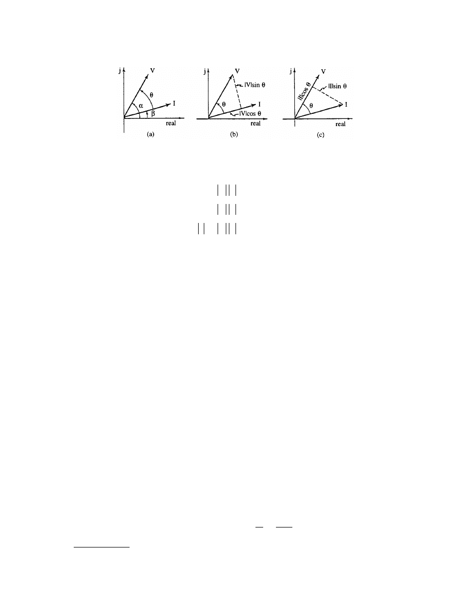
Phasor and Power Diagrams
An interpretation useful for clarifying and understanding the preceding relationships and for the calculation
of power is a graphical approach.
is a phasor diagram of V and I in a particular case. The phasor
voltage can be resolved into two components, one parallel to the phasor current (or in phase with I) and another
perpendicular to the current (or in quadrature with it). This is illustrated in
. Hence, the average
power P is the magnitude of phasor I multiplied by the in-phase component of V; the reactive power Q is the
magnitude of I multiplied by the quadrature component of V.
Alternatively, one can imagine resolving phasor I into two components, one in phase with V and one in
quadrature with it, as illustrated in
. Then P is the product of the magnitude of V with the in-phase
component of I, and Q is the product of the magnitude of V with the quadrature component of I. Real power
is produced only by the in-phase components of V and I. The quadrature components contribute only to the
reactive power.
The in-phase or quadrature components of V and I do not depend on the specific values of the angles of
each, but on their phase difference. One can imagine the two phasors in the preceding diagram to be rigidly
held together and rotated around the origin by any angle. As long as the angle
q is held fixed, all of the discussion
of this section will still apply. It is common to take the current phasor as the reference for angle; that is, to
choose
b = 0 so that phasor I lies along the real axis. Then q = a.
Power Factor
For any given circuit it is useful to know what part of the total complex power is real (average) power and what
part is reactive power. This is usually expressed in terms of the
p
, defined as the ratio of real
power to apparent power:
(3.9)
FIGURE 3.22
In-phase and quadrature components of V and I.
P
V I
Q
V I
S
V I
=
( )
=
( )
=
( )
cos
sin
q
q
a
b
c
Power factor =×
=
=
F
P
S
P
V I
p
* * * ** *
© 2000 by CRC Press LLC
Not counting the right side, this is a general relationship, although we developed it here for sinusoidal excita-
tions. With P =
*V**I* cos q, we find that the power factor is simply cos q. Because of this, q itself is called the
power factor angle.
Since the cosine is an even function [cos(–
q) = cos q], specifying the power factor does not reveal the sign
of
q. Remember that q is the angle of the impedance. If q is positive, this means that the current lags the voltage;
we say that the power factor is a lagging power factor. On the other hand, if
q is negative, the current leads the
voltage and we say this represent a leading power factor.
The power factor will reach its maximum value, unity, when the voltage and current are in phase. This will
happen in a purely resistive circuit, of course. It will also happen in more general circuits for specific element
values and a specific frequency.
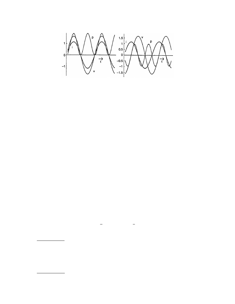
We can now obtain a physical interpretation for the reactive power. When the power factor is unity, the
voltage and current are in phase and sin
q = 0. Hence, the reactive power is zero. In this case, the instantaneous
power is never negative. This case is illustrated by the current, voltage, and power waveforms in
power curve never dips below the axis, and there is no exchange of energy between the source and the circuit.
At the other extreme, when the power factor is zero, the voltage and current are 90
° out of phase and sin q =
1. Now the reactive power is a maximum and the average power is zero. In this case, the instantaneous power
is positive over half a cycle (of the voltage) and negative over the other half. All the energy delivered by the
source over half a cycle is returned to the source by the circuit over the other half.
It is clear, then, that the reactive power is a measure of the exchange of energy between the source and the
circuit without being used by the circuit. Although none of this exchanged energy is dissipated by or stored in
the circuit, and it is returned unused to the source, nevertheless it is temporarily made available to the circuit
by the source.
1
Average Stored Energy
The average ac energy stored in an inductor or a capacitor can be established by using the expressions for the
instantaneous stored energy for arbitrary time functions in Eq. (3.2), specifying the time function to be
sinusoidal, and taking the average value of the result.
(3.10)
1
Power companies charge their industrial customers not only for the average power they use but for the reactive power
they return. There is a reason for this. Suppose a given power system is to deliver a fixed amount of average power at a
constant voltage amplitude. Since P =
*V**I* cos q, the current will be inversely proportional to the power factor. If the
reactive power is high, the power factor will be low and a high current will be required to deliver the given power. To carry
a large current, the conductors carrying it to the customer must be correspondingly larger and better insulated, which means
a larger capital investment in physical plant and facilities. It may be cost effective for customers to try to reduce the reactive
power they require, even if they have to buy additional equipment to do so.
FIGURE 3.23
Power waveform for unity and zero power factors.
W
L I
W
C V
L
C
=
=
1
2
1
2
2
2
* * * *
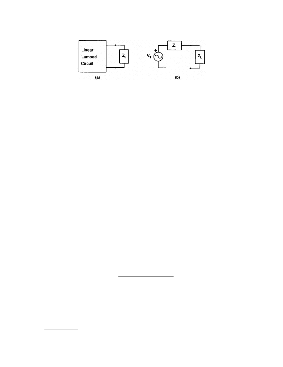
© 2000 by CRC Press LLC
Application of Tellegen’s Theorem to Complex Power
An example of two topologically equivalent networks was shown in
. Let us now specify that two such
networks are linear, all sources are same-frequency sinusoids, they are operating in the steady state, and all
variables are phasors. Furthermore, suppose the two networks are the same, except that the sources of network b
have phasors that are the complex conjugates of those of network a. Then, if V and I denote the vectors of
branch voltages and currents of network a, Tellegen’s theorem in Eq. (3.3) becomes:
(3.11)
where V* is the conjugate transpose of vector V.
This result states that the sum of the complex power delivered to all branches of a linear circuit operating
in the ac steady state is zero. Alternatively stated, the total complex power delivered to a network by its sources
equals the sum of the complex power delivered to its nonsource branches. Again, this result is not surprising.
Since, if a complex quantity is zero, both the real and imaginary parts must be zero, the same result can be
stated for the average power and for the reactive power.
Maximum Power Transfer
The diagram in
illustrates a two-terminal linear circuit at whose terminals an impedance Z
L
is
connected. The circuit is assumed to be operating in the ac steady state. The problem to be addressed is this:
given the two-terminal circuit, how can the impedance connected to it be adjusted so that the maximum
possible average power is transferred from the circuit to the impedance?
The first step is to replace the circuit by its Thévenin equivalent, as shown in Fig. 3.24(b). The current phasor
in this circuit is I = V
T
/(Z
T
+ Z
L
). The average power transferred by the circuit to the impedance is:
(3.12)
In this expression, only the load (that is, R
L
and X
L
) can be varied. The preceding equation, then, expresses a
dependent variable (P) in terms of two independent ones (R
L
and X
L
).
What is required is to maximize P. For a function of more than one variable, this is done by setting the
partial derivatives with respect to each of the independent variables equal to zero; that is,
¶P/¶R
L
= 0 and
¶P/¶X
L
= 0. Carrying out these differentiations leads to the result that maximum power will be transferred
when the load impedance is the conjugate of the Thévenin impedance of the circuit: Z
L
= Z*
T
. If the Thévenin
impedance is purely resistive, then the load resistance must equal the Thévenin resistance.
FIGURE 3.24
A linear circuit delivering power to a load in the steady state.
V I V I
j
j
j
* *
all
·
å
=
= 0
P
I
Z
V
Z
Z
Z
V
R
R
R
X
X
L
T
L
T
L
T
L
T
L
T
L
=
=
+
=
+
+
+
* *
* *
*
*
* *
2
2
2
2
2
2
Re( )
Re( )
)
(
)
(
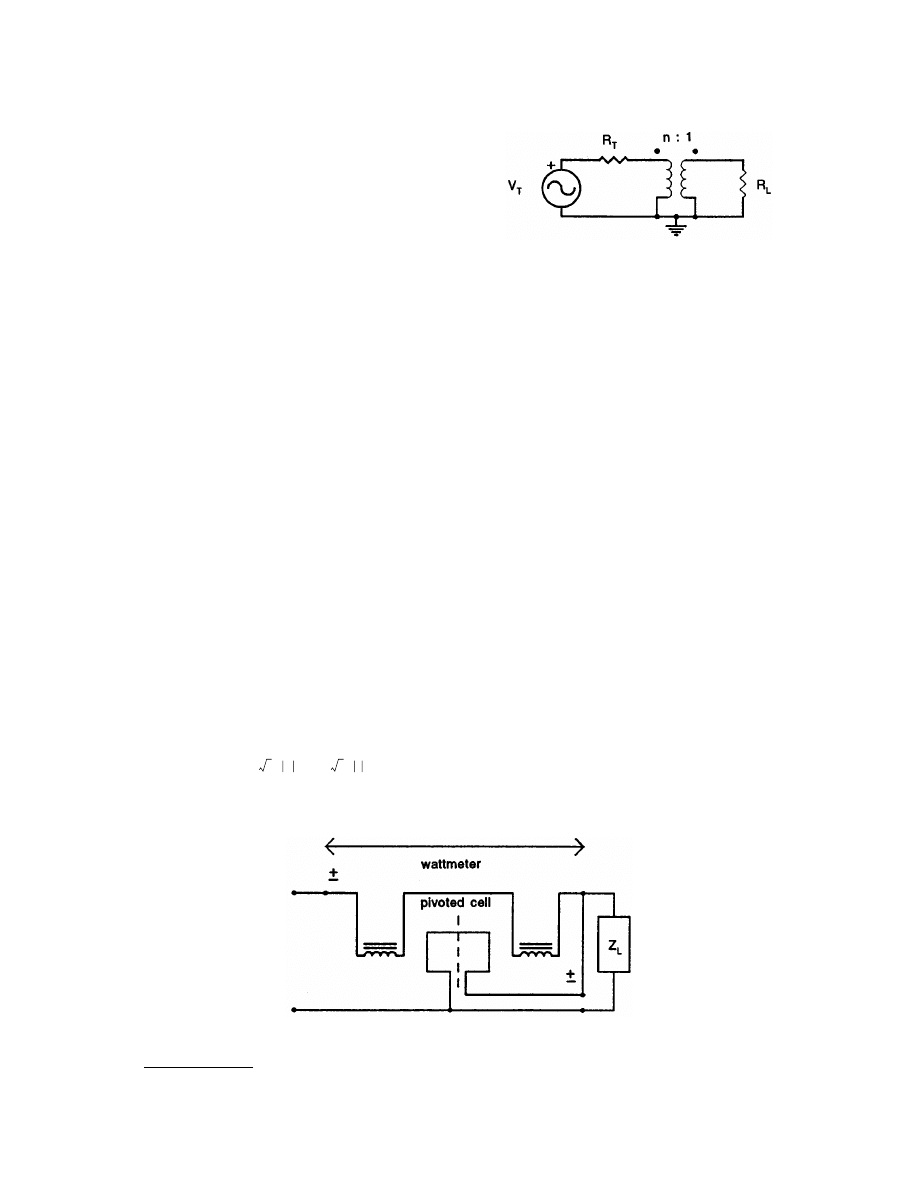
© 2000 by CRC Press LLC
In some cases, both the load impedance and the Thévenin
impedance of the source may be fixed. In such a case, the
matching for maximum power transfer can be achieved by
using a transformer, as illustrated in
, where the
impedances are both resistive. The transformer is assumed
to be ideal, with turns ratio n. Maximum power is trans-
ferred if n
2
= R
T
/R
L
.
Measuring AC Power and Energy
With ac steady-state average power given in the first line of Eq. (3.6), measuring the average power requires
measuring the rms values of voltage and current, as well as the power factor. This is accomplished by the
arrangement shown in
, which includes a breakout of an electrodynamometer-type wattmeter. The
current in the high-resistance pivoted coil is proportional to the voltage across the load. The current to the
load and the pivoted coil together through the energizing coil of the electromagnet establishes a proportional
magnetic field across the cylinder of rotation of the pivoted coil. the torque on the pivoted coil is proportional
to the product of the magnetic field strength and the current in the pivoted coil. If the current in the pivoted
coil is negligible compared to that in the load, then the torque becomes essentially proportional to the product
of the voltage across the load (equal to that across the pivoted coil) and the current in the load (essentially
equal to that through the energizing coil of the electromagnet). The dynamics of the pivoted coil together with
the restraining spring, at ac power frequencies, ensures that the angular displacement of the pivoted coil becomes
proportional to the average of the torque or, equivalently, the average power.
One of the most ubiquitous of electrical instruments is the induction-type watthour meter, which measures
the energy delivered to a load. Every customer of an electrical utility has one, for example. In this instance the
pivoted coil is replaced by a rotating conducting (usually aluminum) disk as shown in
. An induced
eddy current in the disk replaces the pivoted coil current interaction with the load-current-established magnetic
field. After compensating for the less-than-ideal nature of the electrical elements making up the meter as just
described, the result is that the disk rotates at a rate proportional to the average power to the load and the
rotational count is proportional to the energy delivered to the load.
At frequencies above the ac power frequencies and, in some instances, at the ac power frequencies, electronic
instruments are available to measure power and energy. They are not a cost-effective substitute for these meters
in the monitoring of power and energy delivered to most of the millions upon millions of homes and businesses.
Defining Terms
AC steady-state power:
Consider an ac source connected at a pair of terminals to an otherwise isolated
network. Let
and denote the peak values, respectively, of the ac steady-state voltage and
current at the terminals. Furthermore, let
q denote the phase angle by which the voltage leads the current.
Then the average power delivered by the source to the network would be expressed as P =
*V* · *I* cos(q).
FIGURE 3.26
A wattmeter connected to a load.
FIGURE 3.25
Matching with an ideal transformer.
2
V
×
2 I
×
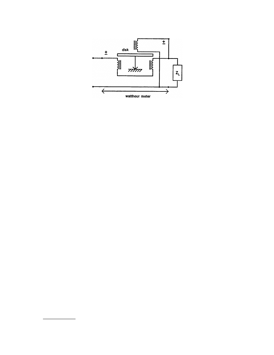
© 2000 by CRC Press LLC
Power and energy:
Consider an electrical source connected at a pair of terminals to an otherwise isolated
network. Power, denoted by p, is the time rate of change in the energy delivered to the network by the
source. This can be expressed as p = vi, where v, the voltage across the terminals, is the energy expended
per unit charge in moving the charge between the pair of terminals and i, the current through the
terminals, is the time rate of charge motion.
Power factor:
Consider an ac source connected at a pair of terminals to an otherwise isolated network. The
power factor, the ratio of the real power to the apparent power
*V* · *I*, is easily established to be cos(q),
where
q is the power factor angle.
Reactive power:
Consider an ac source connected at a pair of terminals to an otherwise isolated network.
The reactive power is a measure of the energy exchanged between the source and the network without
being dissipated in the network. The reactive power delivered would be expressed as Q =
*V* · *I* sin(q).
Real power:
Consider an ac source connected at a pair of terminals to an otherwise isolated network. The
real power, equal to the average power, is the power dissipated by the source in the network.
Tellegen’s theorem:
Two networks, here including all sources, are topologically equivalent if they are similar
structurally, component by component. Tellegen’s theorem states that the sum over all products of the
product of the current of a component of ne network, network a, and of the voltage of the corresponding
component of the other network, network b, is zero. This would be expressed as
S
all j
v
bj
i
aj
= 0. From this
general relationship it follows that in any electrical network, the sum of the power supplied by the sources
is equal to the sum of the power delivered to all the nonsource components.
Related Topic
3.3 Network Theorems
References
N. Balabanian, Electric Circuits, New York: McGraw-Hill, 1994.
A. E. Fitzgerald, D. E. Higginbotham, and A. Grabel, Basic Electrical Engineering, 5th ed., New York: McGraw-
Hill, 1981.
W. H. Hayt, Jr. and J. E. Kemmerly, Engineering Circuit Analysis, 4th ed., New York: McGraw-Hill, 1986.
J. D. Irwin, Basic Engineering Circuit Analysis, New York: Macmillan, 1995.
D. E. Johnson, J. L. Hilburn, and J. R. Johnson, Basic Electric Circuit Analysis, 3rd ed., Englewood Cliffs, N.J.:
Prentice-Hall, 1990.
T. N. Trick, Introduction to Circuit Analysis, New York: John Wiley, 1977.
FIGURE 3.27
A watthour meter connected to a load.
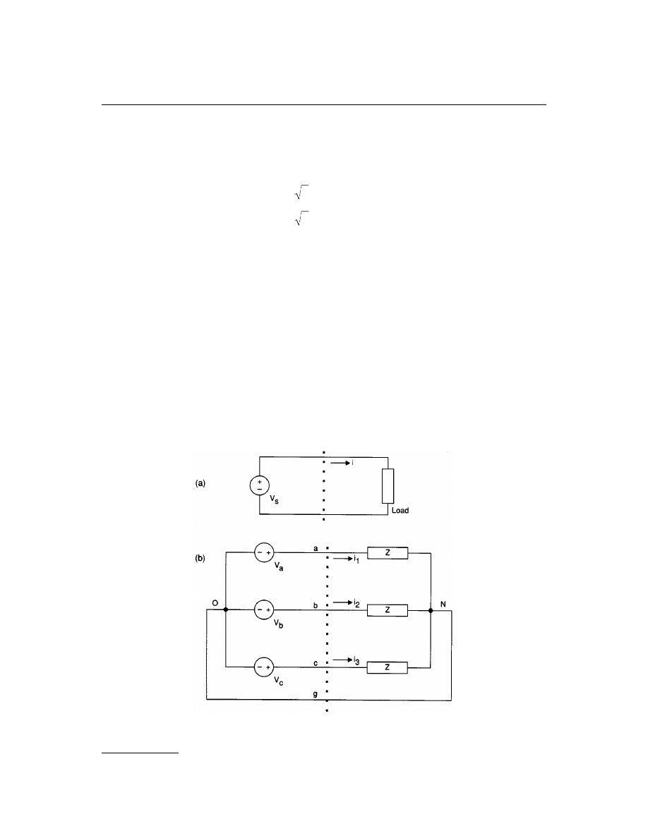
© 2000 by CRC Press LLC
3.5 Three-Phase Circuits
Norman Balabanian
represents the basic circuit for considering the flow of power from a single sinusoidal source to
a load. The power can be thought to cross an imaginary boundary surface (represented by the dotted line in
the figure) separating the source from the load. Suppose that:
(3.13)
Then the power to the load at any instant of time is
p(t) =
*V * *I * [cos(a – b) + cos (2wt + a + b)] (3.14)
The instantaneous power has a constant term and a sinusoidal term at twice the frequency. The quantity in
brackets fluctuates between a minimum value of cos(
a – b) – 1 and a maximum value of cos(a – b) + 1. This
fluctuation of power delivered to the load has certain disadvantages in some situations where the transmission
of power is the purpose of a system. An electric motor, for example, operates by receiving electric power and
transmitting mechanical (rotational) power at its shaft. If the electric power is delivered to the motor in spurts,
the motor is likely to vibrate. In order to run satisfactorily, a physically larger motor will be needed, with a
larger shaft and flywheel, to provide inertia than would be the case if the delivered power were constant.
This problem is overcome in practice by the use of what is called a three-phase system. This section will
provide a brief discussion of three-phase systems.
Consider the circuit in
. This arrangement is similar to a combination of three of the simple
circuits in Fig. 3.28(a) connected in such a way that each one shares the return connection from O to N. The
three sources can be viewed collectively as a single source and the three loads—which are assumed to be
FIGURE 3.28
Flow of power from source to load.
v t V t
i t I t
( ) cos( )
( ) cos( )
=
+
=
+
2
2
* *
* *
w
a
w
b
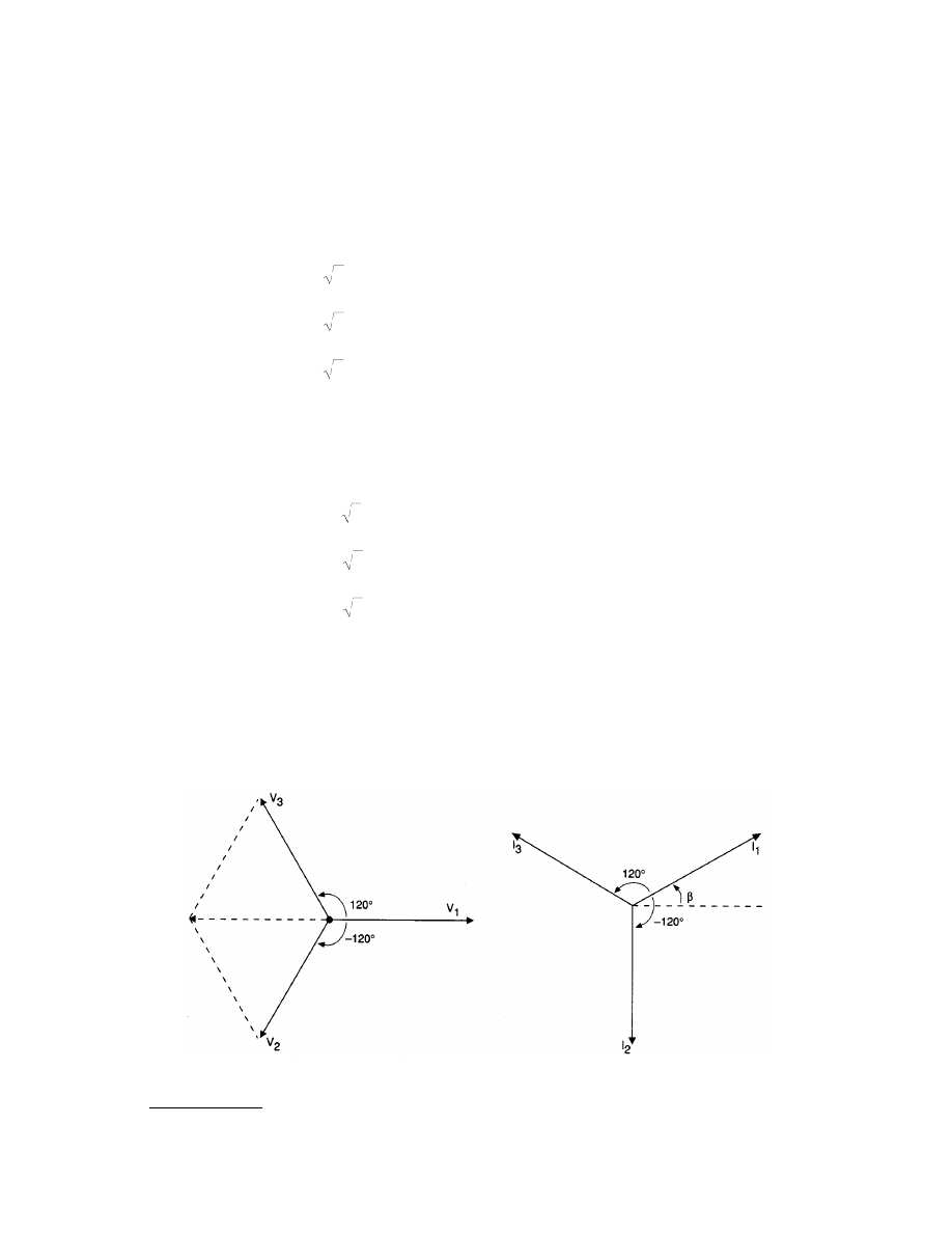
© 2000 by CRC Press LLC
identical—can be viewed collectively as a single load. Then, as before, the dotted line represents a surface
separating the source from the load. Each of the individual sources and loads is referred to as one phase of the
three-phase system.
The three sources are assumed to have the same frequency; they are said to be synchronized. It is also assumed
that the three voltages have the same rms values and the phase difference between each pair of voltages is
±120°
(2
p/3 rad). Thus, they can be written:
(3.15)
The
representing the sinusoids have also been shown. For convenience, the angle of v
a
has been
chosen as the reference for angles; v
b
lags v
a
by 120
° and v
c
leads v
a
by 120
°.
Because the loads are identical, the rms values of the three currents shown in the figure will also be the same
and the phase difference between each pair of them will be
±120°. Thus, the currents can be written:
(3.16)
Perhaps a better form for visualizing the voltages and currents is a graphical one. Phasor diagrams for the
voltages separately and the currents separately are shown in
. The value of angle
b
1
will depend on the
load. An interesting result is clear from these diagrams. First, V
2
and V
3
are each other’s conjugates. So if we
add them, the imaginary parts cancel and the sum will be real, as illustrated by the construction in the voltage
diagram. Furthermore, the construction shows that this real part is negative and equal in size to V
1
. Hence, the
sum of the three voltages is zero. The same is true of the sum of the three currents, as can be established
graphically by a similar construction.
FIGURE 3.29
Voltage and current phasor diagrams.
v
V
t
V
V e
v
V
t
V
V e
v
V
t
V
V e
a
a
j
b
b
j
c
c
j
=
+
«
=
=
+
«
=
=
+
«
=
°
°
°
2
2
2
1
0
2
120
3
120
* * * *
* * * *
* * * *
cos( )
cos( )
cos( )
–
w
a
w
a
w
a
i
I
t
I
I e
i
I
t
I
I e
i
I
t
I
I e
j
j
j
1
1
1
2
2
2
120
3
3
3
120
2
2
2
1
1
1
=
+
«
=
=
+
«
=
=
+
«
=
°
+
°
* * * *
* * * *
* * * *
cos( )
cos( )
cos( )
(
–
)
(
)
w
b
w
b
w
b
b
b
b
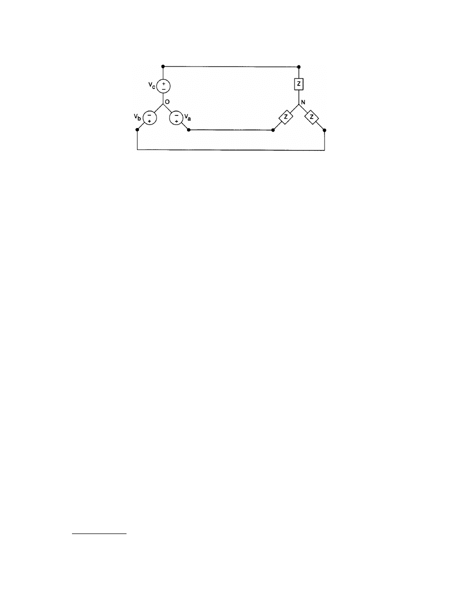
© 2000 by CRC Press LLC
By Kirchhoff ’s current law applied at node N in Fig. 3.28(b), we find that the current in the return line is
the sum of the three currents in Eq. (3.16). However, since this sum was found to be zero, the return line carries
no current. Hence it can be removed entirely without affecting the operation of the system. The resulting circuit
is redrawn in
. Because of its geometrical form, this connection of both the sources and the loads is
said to be a wye (Y) connection.
The instantaneous power delivered by each of the sources has the form given in Eq. (3.14), consisting of a
constant term representing the average power and a double-frequency sinusoidal term. The latter, being
sinusoidal, can be represented by a phasor also. The only caution is that a different frequency is involved here,
so this power phasor should not be mixed with the voltage and current phasors in the same diagram or
calculations. Let
*S* = *V**I* be the apparent power delivered by each of the three sources and let the three power
phasors be S
a
, S
b
, and S
c
, respectively. Then:
(3.17)
It is evident that the phase relationships among these three phasors are the same as the ones among the
voltages and the currents. That is, the second leads the first by 120
° and the third lags the first by 120°. Hence,
just like the voltages and the currents, the sum of these three phasors will also be zero. This is a very significant
result. Although the instantaneous power delivered by each source has a constant component and a sinusoidal
component, when the three powers are added, the sinusoidal components add to zero, leaving only the constants.
Thus, the total power delivered to the three loads is constant.
To determine the value of this constant power, use Eq. (3.14) as a model. The contribution of the kth source
to the total (constant) power is
*S* cos(a
k
–
b
k
). One can easily verify that
a
k
–
b
k
=
a
1
–
b
1
= –
b
1
. The first
equality follows from the relationships among the
a’s from Eq. (3.15) and among the b’s from Eq. (3.16). The
choice of
a
1
= 0 leads to the last equality. Hence, the constant terms contributed to the power by each source
are the same. If P is the total average power, then:
P = P
a
+ P
b
+ P
c
= 3P
a
= 3
*V * *I * cos(a
1
–
b
1
) (3.18)
Although the angle
a
1
has been set equal to zero, for the sake of generality we have shown it explicitly in this
equation.
What has just been described is a balanced three-phase three-wire power system. The three sources in practice
are not three independent sources but consist of three different parts of the same generator. The same is true
FIGURE 3.30
Wye-connected three-phase system.
S
S e
S e
S
S e
S e
S e
S
S e
S e
S e
a
j
j
b
j
j
j
c
j
j
j
=
=
=
=
=
=
=
=
+
+
° +
°
+
°
+
+
° +
+
°
°
* * * *
* * * * * *
* * * * * *
(
)
(
)
(–
–
)
(
)
(
)
(
)
(
–
)
a
b
b
a
b
b
b
a
b
b
b
1
1
1
2
2
1
1
3
3
1
1
120 120 120
120 120 120
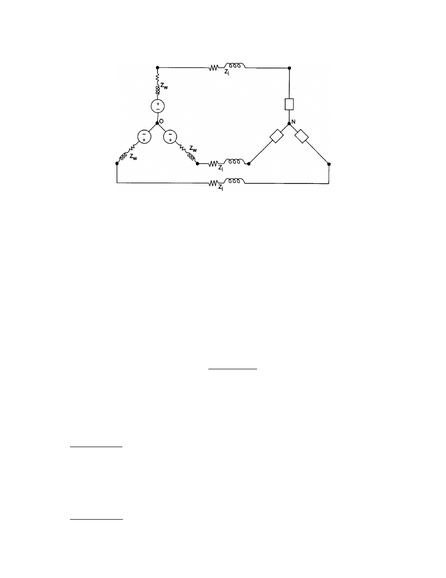
© 2000 by CRC Press LLC
of the loads.
1
What has been described is ideal in a number of ways. First, the circuit can be unbalanced—for
example, by the loads being somewhat unequal. Second, since the real devices whose ideal model is a voltage
source are coils of wire, each source should be accompanied by a branch consisting of the coil inductance and
resistance. Third, since the power station (or the distribution transformer at some intermediate point) may be
at some distance from the load, the parameters of the physical line carrying the power (the line inductance and
resistance) must also be inserted in series between the source and the load.
For an unbalanced system, the analysis of this section does not apply. An entirely new analytical technique
is required to do full justice to such a system.
2
However, an understanding of balanced circuits is a prerequisite
for tackling the unbalanced case.
The last two of the conditions that make the circuit less than ideal (line and source impedances) introduce
algebraic complications, but nothing fundamental is changed in the preceding theory. If these two conditions
are taken into account, the appropriate circuit takes the form shown in
. Here the internal impedance
of a source and the line impedance connecting that source to its load are both connected in series with the
corresponding load. Thus, instead of the impedance in each phase being Z, it is Z + Z
w
+ Z
l
, where w and l are
subscripts standing for “winding” and “line,” respectively. Hence, the rms value of each current is
(3.19)
instead of
*V*/*Z*. All other results we had arrived at remain unchanged. namely, that the sum of the phase
currents is zero and that the sum of the phase powers is a constant. The detailed calculations simply become
a little more complicated.
One other point, illustrated for the loads in
, should be mentioned. Given wye-connected sources
or loads, the wye and the
can be made equivalent by proper selection of the arms of the delta. Thus,
1
An ac power generator consists of (a) a rotor, which produces a magnetic field and which is rotated by a prime mover
(say a turbine), and (b) a stator on which are wound one or more coils of wire. In three-phase systems, the number of coils
is three. The rotating magnetic field induces a voltage in each of the coils. The 120
° leading and lagging phase relationships
among these voltages are obtained by distributing the conductors of the coils around the circumference of the stator so that
they are separated geometrically by 120
°. Thus, the three sources described in the text are in reality a single physical device,
a single generator. Similarly, the three loads might be the three windings on a three-phase motor, again a single physical device.
2
The technique for analyzing unbalanced circuits utilizes what are called symmetrical components.
FIGURE 3.31
Three-phase circuit with nonzero winding and line impedances.
* *
* *
*
*
I
V
Z
Z
Z
w
l
=
+
+

© 2000 by CRC Press LLC
either the sources in Fig. 3.30 or the loads, or both, can be replaced by a delta equivalent; thus we can conceive
of four different three-phase circuits; wye-wye, delta-wye, wye-delta, and delta-delta. Not only can we conceive
of them, they are extensively used in practice.
It is not worthwhile to carry out detailed calculations for these four cases. Once the basic properties described
here are understood, one should be able to make the calculations. Observe, however, that in the delta structure,
there is no neutral connection, so the phase voltages cannot be measured. The only voltages that can be measured
are the line-to-line or simply the line voltages. These are the differences of the phase voltages taken in pairs, as
is evident from Fig. 3.31.
Defining Terms
Delta connection:
The sources or loads in a three-phase system connected end-to-end, forming a closed path,
like the Greek letter
D.
Phasor:
A complex number representing a sinusoid; its magnitude and angle are the rms value and phase of
the sinusoid, respectively.
Wye connection:
The three sources or loads in a three-phase system connected to have one common point,
like the letter Y.
Related Topic
9.2 Three-Phase Connections
References
V. del Toro, Electric Power Systems, Englewood Cliffs, N.J.: Prentice-Hall, 1992.
B.R. Gungor, Power Systems, San Diego: Harcourt Brace Jovanovich, 1988.
P.Z. Peebles and T.A. Giuma, Principles of Electrical Engineering, New York: McGraw-Hill, 1991.
J.J. Grainger and W.D. Stevenson, Jr., Power Systems Analysis, New York: McGraw-Hill, 1994.
G.T. Heydt, Electric Power Quality, Stars in a Circle Publications, 1996.
B.S. Guru and H.R. Hirizoglu, Electric Machinery and Transformers, Saunders, 1996.
3.6 Graph Theory
1
Shu-Park Chan
Topology is a branch of mathematics; it may be described as “the study of those properties of geometric forms
that remain invariant under certain transformations, as bending, stretching, etc.”
2
Network topology (or
1
Based on S.-P. Chan, “Graph theory and some of its applications in electrical network theory,” in Mathematical Aspects
of Electrical Network Analysis, vol. 3, SIAM/AMS Proceedings, American Mathematical Society, Providence, R.I., 1971. With
permission.
2
This brief description of topology is quoted directly from the Random House Dictionary of the English Language, Random
House, New York, 1967.
FIGURE 3.32
Wye connection and delta connection.
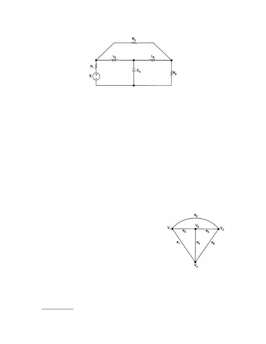
© 2000 by CRC Press LLC
network graph theory) is a study of (electrical) networks in connection with their nonmetric geometrical
(namely topological) properties by investigating the interconnections between the branches and the nodes of
the networks. Such a study will lead to important results in network theory such as algorithms for formulating
network equations and the proofs of various basic network theorems [Chan, 1969; Seshu and Reed, 1961].
The following are some basic definitions in network graph theory, which will be needed in the development
of topological formulas in the analysis of linear networks and systems.
A
(or simply a graph) is a set of line segments called edges and points called vertices, which are
the endpoints of the edges, interconnected in such a way that the edges are connected to (or incident with) the
vertices. The degree of a vertex of a graph is the number of edges incident with that vertex.
A subset G
i
of the edges of a given graph G is called a
of G. If G
i
does not contain all of the edges
of G, it is a
of G. A
is a subgraph having all vertices of degree 2 except for the two
endpoints, which are of degree 1 and are called the terminals of the path. The set of all edges in a path constitutes
a
. If the two terminals of a path coincide, the path is a closed path and is called a
The set of all edges contained in a circuit is called a
A graph or subgraph is said to be
if there is at least one path between every pair of its vertices.
of a connected graph G is a connected subgraph which contains all the vertices of G but no circuits.
The edges contained in a tree are called the
. A 2-tree of a connected graph G is a (proper)
subgraph of G consisting of two unconnected circuitless subgraphs, each subgraph itself being connected, which
together contain all the vertices of G. Similarly, a k-tree is a subgraph of k unconnected circuitless subgraphs,
each subgraph being connected, which together include all the vertices of G. The
is the product of the admittances of all the branches of the k-tree.
Example 3.5. The graph G shown in
is the graph of the
network N of
. The edges of G are e
1
, e
2
, e
4
, e
5
, and e
6
; the vertices
of G are V
1
, V
2
, and V
3
, and V
4
. A path of G is the subgraph G
1
consisting
of edges e
2
, e
3
, and e
6
with vertices V
2
and V
4
as terminals. Thus, the set
{e
2
, e
3
, e
6
} is a path-set. With edge e
4
added to G
1
, we form another
subgraph G
2
, which is a circuit since as far as G
2
is concerned all its
vertices are of degree 2. Hence the set {e
2
, e
3
, e
4
, e
6
} is a circuit-set.
Obviously, G is a connected graph since there exists a path between every
pair of vertices of G. A tree of G may be the subgraph consisting of edges
e
1
, e
4
, and e
6
. Two other trees of G are {e
2
, e
5
, e
6
} and {e
3
, e
4
, e
5
}. A 2-tree
of G is {e
2
, e
4
}; another one is {e
3
, e
6
}; and still another one is {e
3
, e
5
}.
Note that both {e
2
, e
4
} and {e
3
, e
6
} are subgraphs which obviously satisfy
the definition of a 2-tree in the sense that each contains two disjoint
circuitless connected subgraphs, both of which include all the four ver-
tices of G. Thus, {e
3
, e
5
} does not seem to be a 2-tree. However, if we
agree to consider {e
3
, e
5
} as a subgraph which contains edges e
3
and e
5
plus the isolated vertex V
4
, we see that
{e
3
, e
5
} will satisfy the definition of a 2-tree since it now has two circuitless connected subgraphs with e
3
and
e
5
forming one of them and the vertex V
4
alone forming the other. Moreover, both subgraphs together indeed
FIGURE 3.33
A passive network N with a voltage driver E.
FIGURE 3.34
The graph G of the net-
work N of Fig. 3.33.
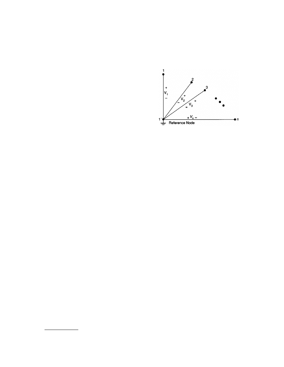
© 2000 by CRC Press LLC
include all the four vertices of G. It is worth noting that a 2-tree is obtained from a tree by removing any one
of the branches from the tree; in general, a k-tree is obtained from a (k – 1) tree by removing from it any one
of its branches. Finally, the tree admittance product of the tree {e
2
, e
5
, e
6
} is
1
/
2
1
/
5
1
/
6
; the 2-tree admittance
product of the 2-tree {e
3
, e
5
} is
1
/
3
1
/
5
(with the admittance of a vertex defined to be 1).
The k-Tree Approach
The development of the analysis of passive electrical networks
using topological concepts may be dated back to 1847 when
Kirchhoff formulated his set of topological formulas in terms
of resistances and the branch-current system of equations. In
1892, Maxwell developed another set of topological formulas
based on the k-tree concept, which are the duals of Kirch-
hoff ’s. These two sets of formulas were supported mainly by
heuristic reasoning and no formal proofs were then available.
In the following we shall discuss only Maxwell’s topological
formulas for linear networks without mutual inductances.
Consider a network N with n independent nodes as shown
¢ is taken as reference (datum) node.
the voltages V
1
, V
2
, . . ., V
n
(which are functions of s) are the
transforms of the node-pair voltages (or simply node voltages) v
1
, v
2
, . . ., v
n
(which are function s of t) between
the n nodes and the reference node 1
¢ with the plus polarity marks at the n nodes. It can be shown [Aitken,
1956] that the matrix equation for the n independent nodes of N is given by
(3.20)
or, in abbreviated matrix notation,
Y
n
V
n
= I
n
(3.21)
where Y
n
is the node admittance matrix, V
n
the n
´ 1 matrix of the node voltage transforms, and I
n
the n
´ 1
matrix of the transforms of the known current sources.
For a relaxed passive one-port (with zero initial conditions) shown in
, the driving-point impedance
function Z
d
(s) and its reciprocal, namely driving-point admittance function Y
d
(s), are given by
Z
d
(s) = V
1
/I
1
=
D
11
/
D
and
Y
d
(s) = 1/Z
d
(s) =
D/D
11
respectively, where
D is the determinant of the node admittance matrix Y
n
, and
D
11
is the (1,1)-cofactor of
D.
Similarly, for a passive reciprocal RLC two-port (
), the open-circuit impedances and the short-circuit
admittances are seen to be
z
11
=
D
11
/
D (3.22a)
FIGURE 3.35
A network N with n independent
nodes.
y
y
y
y
y
y
y
y
y
V
V
V
I
I
I
n
n
n
n
nn
n
n
11 12 1
21 22 2
1
2
1
2
1
2
× × ×
× × ×
× × ×
é
ë
ê
ê
ê
ê
ê
ù
û
ú
ú
ú
ú
ú
é
ë
ê
ê
ê
ê
ê
ù
û
ú
ú
ú
ú
ú
=
é
ë
ê
ê
ê
ê
ê
ù
û
ú
ú
ú
ú
ú
M
M
M
M
M
M
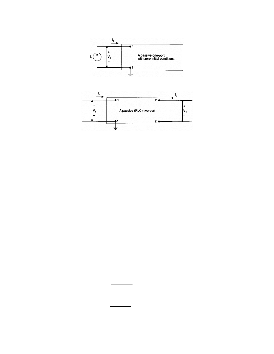
© 2000 by CRC Press LLC
z
12
= z
21
= (
D
12
–
D
12
¢
)/
D (3.22b)
z
22
= (
D
22
+
D
2
¢2¢
– 2
D
22
¢
)/
D (3.22c)
and
y
11
= (
D
22
+
D
2
¢2¢
– 2
D
22
¢
)/(D
1122
+
D
112
¢2¢
– 2
D
1122
¢
) (3.23a)
y
12
= y
21
=
D
12
¢
–
D
12
/(
D
1122
+
D
112
¢2¢
– 2
D
1122
¢
) (3.23b)
y
22
=
D
11
/(
D
1122
+
D
112
¢2¢
– 2
D
1122
¢
) (3.23c)
respectively, where
D
ij
is the (i,j)-cofactor of
D, and D
ijkm
is the cofactor of
D by deleting rows i and k and columns
j and m from
D [Aitken, 1956].
Expressions in terms of network determinants and cofactors for other network transfer functions are given
by (
(3.24a)
(3.24b)
(3.24c)
(3.24d)
FIGURE 3.36
The network N driven by a single current source.
FIGURE 3.37
A passive two-port.
z
V
I
12
2
1
12 12
=
=
¢
D
D
D
–
(transfer impedance function)
G
V
V
12
2
1
12 12
11
=
=
¢
D
D
D
–
(voltage-ratio transfer function)
Y
Y G
Y
L
L
12
(transfer admittance function)
=
=
æ
è
ç
ö
ø
÷
¢
12
12 12
11
D
D
D
–
a
12
(current-ratio transfer function)
=
=
æ
è
ç
ö
ø
÷
¢
Y Z Y
L
1
12
12 12
D
D
D
–
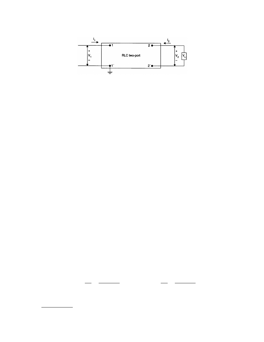
© 2000 by CRC Press LLC
The topological formulas for the various network functions of a passive one-port or two-port are derived
from the following theorems which are stated without proof [Chan, 1969].
Theorem 3.1.
Let N be a passive network without mutual inductances. The determinant
D of the node
admittance matrix Y
n
is equal to the sum of all tree-admittances of N, where a tree-admittance product t
(i)
(y)
is defined to be the product of the admittance of all the branches of the tree T
(i)
. That is,
(3.25)
Theorem 3.2.
Let
D be the determinant of the node admittance matrix Y
n
of a passive network N with n + 1
nodes and without mutual inductances. Also let the reference node be denoted by 1
¢. Then the ( j,j)-cofactor
D
jj
of
D is equal to the sum of all the 2-tree-admittance products T
2 j,1
¢
(y) of N, each of which contains node j
in one part and node 1
¢ as the reference node) and without mutual inductances is given by
(3.26)
where the summation is taken over all the 2-tree-admittance products of the form T
2 j,1
¢
(y).
Theorem 3.3.
The (i,j)-cofactor
D
ij
of
D of a relaxed passive network N with n independent nodes (with node
1
¢ as the reference node) and without mutual inductances is given by
(3.27)
where the summation is taken over all the 2-tree-admittance products of the form T
2 ij,1
¢
(y) with each containing
nodes i and j in one connected port and the reference node 1
¢ in the other.
For example, the topological formulas for the driving-point function of a passive one-port can be readily
obtained from Eqs. (3.25) and (3.26) in Theorems 3.1 and 3.2 as stated in the next theorem.
Theorem 3.4.
With the same notation as in Theorems 3.1 and 3.2, the driving-point admittance Y
d
(s) and
the driving-point impedance Z
d
(s) of a passive one-port containing no mutual inductances at terminals 1 and
1
¢ are given by
(3.28)
respectively.
FIGURE 3.38
A loaded passive two-port.
D =
=
å
det
( )
( )
Y
T
y
n
i
i
D
jj
k
k
T
y
j
=
¢
å
2
1
,
( )
( )
D
ij
k
k
T
y
i j
=
¢
å
2
1
,
( )
( )
Y s
T
y
T
y
Z s
T
y
T
y
d
i
i
k
k
d
k
k
i
i
( )
( )
( )
( )
( )
( )
( )
( )
( )
( )
,
,
=
=
=
=
å
å
å
å
D
D
D
D
11
2
11
2
1 1
1 1
and

© 2000 by CRC Press LLC
For convenience we define the following shorthand notation:
(3.29)
Thus Eq. (3.28) may be written as
Y
d
(s) = V(Y)/W
1,1
¢
(Y)
and
Z
d
(s) = W
1,1
¢
(Y)/V(Y)
(3.30)
In a two-port network N, there are four nodes to be specified, namely, 1 and 1
¢ at the input port (1,1¢) and
nodes 2 and 2
¢ at the output port (2,2¢), as illustrated in Fig. 3.38. However, for a 2-tree of the type T
2 ij,1
¢
, only
three nodes have been used, thus leaving the fourth one unidentified.
With very little effort, it can be shown that, in general, the following relationship holds:
W
ij,1
¢
(Y) = W
ijk,1
¢
(Y) + W
ij,k1
¢
(Y)
or simply
W
ij,1
¢
= W
ijk,1
¢
+ W
ij,k1
¢
(3.31)
where i, j, k, and 1
¢ are the four terminals of N with 1¢ denoting the datum (reference) node. The symbol W
ijk,1
¢
denotes the sum of all the 2-tree-admittance products, each containing nodes i, j, and k in one connected part
and the reference node, 1
¢, in the other.
We now state the next theorem.
Theorem 3.5.
With the same hypothesis and notation as stated earlier in this section,
D
12
–
D
12
¢
= W
12,12
¢
(Y) – W
12
¢,1¢2
(Y)
(3.32)
It is interesting to note that Eq. (3.32) is stated by Percival [1953] in the following descriptive fashion:
which illustrates the two types of 2-trees involved in the formula. Hence, we state the topological formulas for
z
11
, z
12
, and z
22
in the following theorem.
Theorem 3.6.
With the same hypothesis and notation as stated earlier in this section
z
11
= W
1,1
¢
(Y)/V(Y)
(3.33a)
z
12
= z
21
= {W
12,1
¢2¢
(Y) – W
12
¢,1¢2
(Y)}/V(Y)
(3.33b)
z
22
= W
2,2
¢
(Y)/V(Y)
(3.33c)
We shall now develop the topological expressions for the short-circuit admittance functions. Let us denote
by U
a,b,c
(Y) the sum of all 3-tree admittance products of the form T
3a,b,c
(Y) with identical subscripts in both
( ) ( )
( )
( )
( )
( )
,
,
a V Y
T
y
b W
y
T
y
j
r
i
i
j r
j r
k
º
=
º
=
å
å
sum of all tree- admittance products, and
( )
sum of all 2- tree - admittance products with node
and the reference node contained in different parts.
2
D
D
12
12
12 12
12 1 2
1
2
1
2
1
2
1
2
–
–
–
,
,
¢
¢
¢ ¢
=
=
¢
¢
æ
è
ç
ç
ç
ö
ø
÷
÷
÷
¢
¢
æ
è
ç
ç
ç
ö
ø
÷
÷
÷
W
W
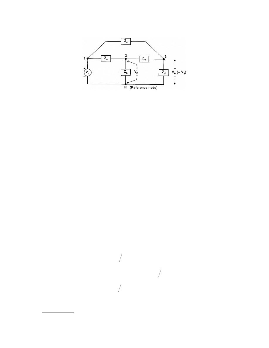
© 2000 by CRC Press LLC
symbols to represent the same specified distribution of vertices. Then, following arguments similar to those of
Theorem 3.5, we readily see that
(3.34a)
(3.34b)
(3.34c)
where 1,1
¢,2,2¢ are the four terminals of the two-port with 1¢ denoting the reference node (
). However,
we note that in Eqs. (3.34a) and (3.34b) only three of the four terminals have been specified. We can therefore
further expand U
1, 2, 1
¢
and U
1, 2
¢, 1¢
to obtain the following:
D
1122
+
D
112
¢2¢
– 2
D
1122
¢
= U
12
¢, 2, 1¢
+ U
1, 2, 1
¢2¢
+ U
12, 2
¢, 1¢
+ U
1, 2
¢, 1¢2
(3.35)
For convenience, we shall use the shorthand notation
SU to denote the sum of the right of Eq. (3.35). Thus,
we define
(3.36)
Hence, we obtain the topological formulas for the short-circuit admittances as stated in the following theorem.
Theorem 3.7.
The short-circuit admittance functions y
11
, y
12
, and y
22
of a passive two-port network with no
mutual inductances are given by
(3.37a)
(3.37b)
(3.37c)
where
SU is defined in Eq. (3.36) above.
Finally, following similar developments, other network functions are stated in Theorem 3.8.
FIGURE 3.39
The network N of Example 3.7.
D
1122 3 1 2 1
1 2 1
=
º
¢
å
¢
T
y
U
Y
i
i
, ,
( )
, ,
( ) ( )
D
112 2 3 1 2 1
1 2 1
¢ ¢ ¢ ¢
=
º
¢
¢
å
T
y
U
Y
j
j
,
,
( )
, ,
( ) ( )
D
1122
3
1 2 2 1
1 2 2 1
¢
¢ ¢
=
º
¢ ¢
å
T
y
U
U
k
k
,
,
( )
,
,
( ) ( )
U
U
U
U
U
=
+
+
+
¢
¢ ¢ ¢ ¢ ¢ ¢ ¢
å
12 2 1 1 2 1 2 12 2 1 1 2 1 2
, , , , , , , ,
y
W
U
11 2 2
=
¢
å
,
y
y
W
W
U
12 21 12 1 2 12 1 2
=
=
-
( )
¢ ¢ ¢ ¢
å
,
,
y
W
U
22 1 1
=
¢
å
,

© 2000 by CRC Press LLC
Theorem 3.8.
With the same notation as before,
(3.38a)
(3.38b)
(3.38c)
(3.38d)
The Flowgraph Approach
Mathematically speaking, a linear electrical network or, more generally, a linear system can be described by a
set of simultaneous linear equations. Solutions to these equations can be obtained either by the method of
successive substitutions (elimination theory), by the method of determinants (Cramer’s rule), or by any of the
topological techniques such as Maxwell’s k-tree approach discussed in the preceding subsection and the flow-
graph techniques represented by the works of Mason [1953, 1956], and Coates [1959].
Although the methods using algebraic manipulations can be amended and executed by a computer, they do
not reveal the physical situations existing in the system. The flowgraph techniques, on the other hand, show
intuitively the causal relationships between the variables of the system of interest and hence enable the network
analyst to have an excellent physical insight into the problem.
In the following, two of the more well-known flowgraph techniques are discussed, namely, the
technique devised by Mason and the method based on the flowgraph of Coates and recently modified
by Chan and Bapna [1967].
A signal-flowgraph G
m
of a system S of n independent linear (algebraic) equations in n unknowns
(3.39)
is a graph with junction points called nodes which are connected by directed line segments called branches with
signals traveling along the branches only in the direction described by the arrows of the branches. A signal x
k
traveling along a branch between x
k
and x
j
is multiplied by the gain of the branches g
kj
, so that a signal of g
kj
x
k
is delivered at node x
j
. An input node (source) is a node which contains only outgoing branches; an output node
(sink) is a node which has only incoming branches. A path is a continuous unidirectional succession of branches,
all of which are traveling in the same direction; a forward path is a path from the input node to the output node
along which all nodes are encountered exactly once; and a feedback path (loop) is a closed path which originates
from and terminates at the same node, and along which all other nodes are encountered exactly once (the trivial
case is a self-loop which contains exactly one node and one branch). A path gain is the product of all the branch
gains of the path; similarly, a loop gain is the product of all the branch gains of the branches in a loop.
The procedure for obtaining the Mason graph from a system of linear algebraic equations may be described
in the following steps:
Z
s
W
W
V
12
12 1 2 12 1 2
( )
–
,
,
=
¢ ¢ ¢ ¢
G
s
W
W
W
12
12 1 2 12 1 2
1 1
( )
–
,
,
,
=
¢ ¢ ¢ ¢
¢
Y
s
Y
W
W
W
L
12
12 1 2 12 1 2
1 1
( )
–
,
,
,
=
¢ ¢ ¢ ¢
¢
a
12
12 1 2 12 1 2
( )
–
,
,
s
Y
W
W
V
L
=
¢ ¢ ¢ ¢
a x b i n
ij j i
j
n
=
=
¼
=
å
1
1 2
, ,
,

© 2000 by CRC Press LLC
a. Arrange all the equations of the system in such a way that the jth dependent (output) variable x
j
in the
jth equation is expressed explicitly in terms of the other variables. Thus, if the system under study is
given by Eq. (3.39), namely
(3.40)
where b
1
,b
2
, . . ., b
n
are inputs (sources) and x
1
, x
2
, . . ., x
n
are outputs, the equations may be rewritten as
(3.41)
b. The number of input nodes in the flowgraph is equal to the number of nonzero b’s. That is, each of the
source nodes corresponds to a nonzero b
j
.
c. To each of the output nodes is associated one of the dependent variables x
1
,x
2
, . . ., x
n
.
d. The value of the variable represented by a node is equal to the sum of all the incoming signals.
e. The value of the variable represented by any node is transmitted onto all branches leaving the node.
It is a simple matter to write the equations from the flowgraph since every node, except the source nodes of
the graph, represents an equation, and the equation associated with node k, for example, is obtained by equating
to x
k
the sum of all incoming branch gains multiplied by the values of the variables from which these branches
originate.
Mason’s general gain formula is now stated in the following theorem.
Theorem 3.9.
Let G be the overall graph gain and G
k
be the gain of the kth forward path from the source to
the sink. Then
(3.42)
where
p
m1
= loop gain (the product of all the branch gains around a loop)
p
m2
= product of the loop gains of the mth set of two nontouching loops
p
m3
= product of the loop gains of the mth set of three nontouching loops, and in general
a x
a x
a x
b
a x
a x
a x
b
a x
a x
a x
b
n
n
n
n
n
n
nn
n
n
11 1
12
2
1
1
21 1
22
2
2
2
1
1
2
2
+
+
+
=
+
+
+
=
+
+
+
=
L
L
M
M
M
M
M
L
x
a
b
a
a
x
a
a
x
a
a
x
x
a
b
a
a
x
a
a
x
a
a
x
x
a
b
a
a
x
a
a
x
a
a
x
n
n
n
n
n
nn
n
n
nn
n
nn
n
n
nn
n
1
11
1
12
11
2
13
11
3
1
11
2
22
2
21
22
1
23
22
3
2
22
1
1
2
2
1
1
1
1
1
=
× × ×
=
× × ×
=
× × ×
–
–
–
–
–
–
–
–
–
–
–
–
– , –
–
M
M
M
M
M
M
1
1
G
G
k
k
k
=
å
1
D
D
D =
+
+ × × × +
å
å
å
å
1
1
1
2
3
p
p
p
p
m
m
m
m
m
j
m
mj
m
–
(– )

© 2000 by CRC Press LLC
p
mj
= product of the loop gains of the mth set of j nontouching loops
D
k
= the value of
D for that subgraph of the graph obtained by removing the kth forward path along with
those branches touching the path
Mason’s signal-flowgraphs constitute a very useful graphical technique for the analysis of linear systems. This
technique not only retains the intuitive character of the block diagrams but at the same time allows one to
obtain the gain between an input node and an output node of a signal-flowgraph by inspection. However, the
derivation of the gain formula [Eq. (3.42)] is by no means simple, and, more importantly, if more than one
input is present in the system, the gain cannot be obtained directly; that is, the principle of superposition must
be applied to determine the gain due to the presence of more than one input. Thus, by slight modification of
the conventions involved in Mason’s signal-flowgraph, Coates [1959] was able to introduce the so-called
“flowgraphs” which are suitable for direct calculation of gain.
Recently, Chan and Bapna [1967] further modified Coates’s flowgraphs and developed a simpler gain formula
based on the modified graphs. The definitions and the gain formula based on the modified Coates graphs are
presented in the following discussion.
The
(called the modified Coates graph) of a system S of n independent linear equations in n
unknowns
is an oriented graph such that the variable x
j
in S is represented by a node (also denoted by x
j
) in G
l
, and the
coefficient a
ij
of the variable x
j
in S by a branch with a branch gain a
ij
connected between nodes x
i
and x
j
in G
l
and directed from x
j
to x
i
. Furthermore, a source node is included in G
l
such that for each constant b
k
in S there
is a node with gain b
k
in G
l
from node 1 to node s
k
. Graph G
l0
is the subgraph of G
l
obtained by deleting the
source node l and all the branches connected to it. Graph G
ij
is the subgraph of G
l
obtained by first removing
all the outgoing branches from node x
j
and then short-circuiting node l to node x
j
. A loop set l is a subgraph
of G
l0
that contains all the nodes of G
l0
with each node having exactly one incoming and one outgoing branch.
The product p of the gains of all the branches in l is called a loop-set product. A 2-loop-set I
2
is a subgraph of
G
lj
containing all the nodes of G
lj
with each node having exactly one incoming and one outgoing branch. The
product p
2
of the gains of all the branches in l
2
is called a 2-loop-set product.
The modified Coates gain formula is now stated in the following theorem.
Theorem 3.10.
In a system of n independent linear equations in n unknowns
the value of the variable x
j
is given by
(3.43)
where N
l 2
is the number of loops in a 2-loop-set l
2
and N
l
is the number of loops in a loop set l.
Since both the Mason graph G
m
and the modified Coates graph G
l
are topological representations of a system
of equations it is logical that certain interrelationships exist between the two graphs so that one can be
transformed into the other. Such interrelationships have been noted [Chan, 1969], and the transformations are
briefly stated as follows:
A. Transformation of G
m
into G
l
.
Graph G
m
can be transformed into an equivalent Coates graph G
l
(representing an equivalent system of equations) by the following steps:
a x b i n
ij
j
n
j
i
=
å
=
=
1
1 2
, ,
,
. . .
a x b i n
ij j i
=
= 1 2
, ,
,
...
x
p
p
j
N
p
N
p
=
å
å
(–1) (–1)
1 2
2
1
2
(all (all
)
)
2

© 2000 by CRC Press LLC
a. Subtract 1 from the gain of each existing self-loop.
b. Add a self-loop with a gain of –1 to each branch devoid of self-loop.
c. Multiply by –b
k
the gain of the branch at the kth source node b
k
(k = 1, 2, . . ., r, r being the number
of source nodes) and then combine all the (r) nodes into one source node (now denoted by 1).
B. Transformation of G
l
into G
m
.
Graph G
l
can be transformed into G
m
by the following steps:
a. Add 1 to the gain of each existing self-loop.
b. Add a self-loop with a gain of 1 to each node devoid of self-loop except the source node l.
c. Break the source node l into r source nodes (r being the number of branches connected to the source
node l before breaking), and identify the r new sources nodes by b
1
,b
2
, . . ., b, with the gain of the
corresponding r branches multiplied by –1/b
1
, –1/b
2
, . . ., –1/b
r
, respectively, so that the new gains
of these branches are all equal to l, keeping the edge orientations unchanged.
The gain formulas of Mason and Coates are the classical ones in the theory of flowgraphs. From the systems
viewpoint, the Mason technique provides an excellent physical insight as one can visualize the signal flow
through the subgraphs (forward paths and feedback loops) of G
m
. The graph reduction technique based on
the Mason graph enables one to obtain the gain expression using a step-by-step approach and at the same time
observe the cause-and-effect relationships in each step. However, since the Mason formula computes the ratio
of a specified output over one particular input, the principle of superposition must be used in order to obtain
the overall gain of the system if more than one input is present. The Coates formula, on the other hand,
computes the output directly regardless of the number of inputs present in the system, but because of such a
direct computation of a given output, the graph reduction rules of Mason cannot be applied to a Coates graph
since the Coates graph is not based on the same cause-effect formulation of equations as Mason’s.
The k-Tree Approach Versus the Flowgraph Approach
When a linear network is given, loop or node equations can be written from the network, and the analysis of
the network can be accomplished by means of either Coates’s or Mason’s technique.
However, it has been shown [Chan, 1969] that if the Maxwell k-tree approach is employed in solving a linear
network, the redundancy inherent either in the direct expansion of determinants or in the flowgraph techniques
described above can be either completely eliminated for passive networks or greatly reduced for active networks.
This point and others will be illustrated in the following example.
Example 3.7. Consider the network N as shown in
. Let us determine the voltage gain, G
12
= V
0
/V
1
,
using (1) Mason’s method, (2) Coates’s method, and (3) the k-tree method.
The two node equations for the network are given by
for node 2: (Y
a
+ Y
b
+ Y
e
)V
2
+ (–Y
3
)V
0
= Y
a
V
i
for node 3: (–Y
e
)V
2
+ (Y
c
+ Y
d
+ Y
e
)V
0
= Y
c
V
i
(3.44)
where
Y
a
= 1/Z
a
, Y
b
= 1/Z
b
, Y
c
= 1/Z
c
, Y
d
= 1/Z
d
and Y
e
= 1/Z
e
(1) Mason’s approach. Rewrite the system of two equations (3.44) as follows:
(3.45)
V
Y
Y
Y
Y
V
Y
Y
Y
Y
V
V
Y
Y
Y
Y
V
Y
Y
Y
Y
V
a
a
b
e
i
e
a
b
e
c
c
d
e
i
e
c
d
e
2
0
0
2
=
+
+
æ
è
ç
ö
ø
÷
+
+
+
æ
è
ç
ö
ø
÷
=
+
+
æ
è
ç
ö
ø
÷
+
+
+
æ
è
ç
ö
ø
÷

© 2000 by CRC Press LLC
or
V
2
= AV
i
+ BV
0
V
0
= CV
i
+ DV
2
(3.46)
where
The Mason graph of system (3.46) is shown in
, and according to the Mason graph formula (3.42),
we have
D = 1 – BD
G
C
= C
D
C
= 1
G
AD
= AD
D
AD
= 1
and hence
Upon cancellation and rearrangement of terms
(3.47)
(2) Coates’s approach. From (3.44) we obtain the Coates graphs G
l
, G
l0
, and G
l3
as shown in
and
, respectively. The set of all loop-sets of G
l 0
is shown in
, and the set of all 2-loop-sets of G
l 3
is
shown in
. Thus, by Eq. (3.43),
FIGURE 3.40
The Mason graph of N.
A
Y
Y
Y
Y
B
Y
Y
Y
Y
C
Y
Y
Y
Y
D
Y
Y
Y
Y
a
a
b
e
e
a
b
e
c
c
d
e
e
c
d
e
=
+
+
=
+
+
=
+
+
=
+
+
G
V
V
G
BD
C
AD
Y
Y
Y
Y
Y
Y
Y
Y
Y
Y
Y
Y
Y
Y
Y
Y
Y
Y
k
k
k
c
c
d
e
a
a
b
e
c
d
e
e
a
b
e
c
d
e
12
0
1
2
1
1
1
1
=
=
=
+
=
+
+
+
+
+
+
+
-
+
+
+
+
å
D
D
–
(
)
/( ) /( )( )
/( )( )
G
Y Y Y Y Y Y Y Y
Y Y Y Y Y Y Y Y Y Y Y Y Y Y Y Y
a
c
a
e
b c
c e
a
c
a
d
a
e
b c
b d
b e
c e
d e
12
=
+
+
+
+
+
+
+
+
+
+
V
p
p
Y
Y V
Y
Y
Y
Y V
Y
Y
Y
Y
Y
Y
Y
Y
N
p
N
p
e
a
i
a
b
e
c
i
e
e
a
b
e
c
d
e
l
l
0
2
1
2
1
2
1
1
1
1
1
1
2
=
=
+
+
+
+
+
+
+
+
å
å
(– )
(– )
(– ) (– )( ) (– ) ( )( )
(– ) (– )(– ) (– ) ( )( )
(
)
(
)
all
all
2
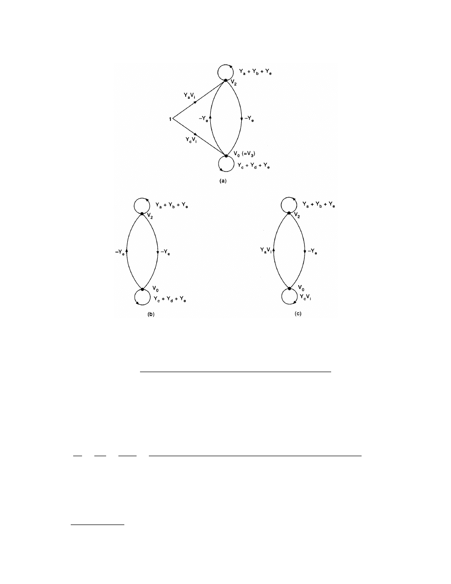
© 2000 by CRC Press LLC
Or, after simplification, we find
(3.48)
which gives the same ratio V
0
/V
i
as Eq. (3.47).
(3) The k-tree approach. Recall that the gain formula for V
0
/V
i
using the k-tree approach is given [Chan,
1969] by
where
D
13
and
D
11
are cofactors of the determinant
D of the node admittance matrix of the network. Furthermore,
it is noted that the 2-trees corresponding to
D
ii
may be obtained by finding all the trees of the modified graph
G
i
, which is obtained from the graph G of the network by short-circuiting node i (i being any node other than
FIGURE 3.41
The Coates graphs: (a) G
l
, (b) G
l 0
, and (c) G
l 3
.
V
Y Y
Y Y
Y Y
Y Y V
Y Y
Y Y
Y Y
Y Y
Y Y
Y Y
Y Y
Y Y
a
c
a
e
b c
c e
i
a
c
a
d
a
e
b c
b d
b e
c e
d
e
0
=
+
+
+
+
+
+
+
+
+
+
(
)
V
V
W
W
i
R
R
R
R
0
13
11
13
1
=
=
=
æ
è
çç
ö
ø
÷÷
æ
è
çç
ö
ø
÷÷
å
å
D
D
,
,
all 2-tree admittance products with nodes 1 and 3 in one part
and the reference node in the other part of each of such 2-tree
all 2-tree admittance products with node 1 in one part and
the reference node in the other part of each of such 2-tree
(3.49)

© 2000 by CRC Press LLC
R) to the reference node R, and that the 2-trees corresponding to
D
ij
can be found by taking all those 2-trees
each of which is a tree of both G
i
and G
j
[Chan, 1969]. Thus, for
D
11
, we first find G and G
1
then find the set S
1
of all trees of G
1
); then for
D
13
, we find G
3
3
of all trees
of G
3
) and then from S
1
and S
3
we find all the terms common to both sets (which correspond to the
FIGURE 3.42
The set of all loop-sets of G
l 0
.
FIGURE 3.43
The set of all 2-loop-sets of G
l 3
.
FIGURE 3.44
(a) Graph G, and (b) the modified graph G
l
of G.
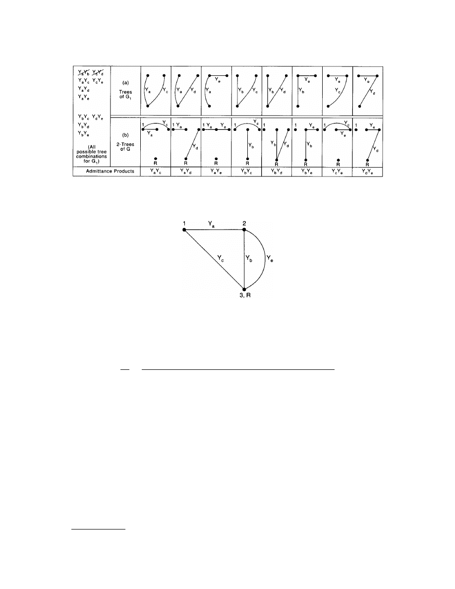
© 2000 by CRC Press LLC
set of all trees common to G
1
and G
3
) as shown in
Finally we form the ratio of 2-tree admittance
products according to Eq. (3.49). Thus from Figs. 3.45 and 3.48, we find
which is identical to the results obtained by the flowgraph techniques.
From the above discussions and Example 3.7 we see that the Mason approach is the best from the systems
viewpoint, especially when a single source is involved. It gives an excellent physical insight to the system and
reveals the cause-effect relationships at various stages when graph reduction technique is employed. While the
Coates approach enables one to compute the output directly regardless of the number of inputs involved in
the system, thus overcoming one of the difficulties associated with Mason’s approach, it does not allow one to
reduce the graph step-by-step toward the final solution as Mason’s does. However, it is interesting to note that
in the modified Coates technique the introduction of the loop-sets (analogous to trees) and the 2-loop-sets
(analogous to 2-trees) brings together the two different concepts—the flowgraph approach and the k-tree
approach.
From the networks point of view, the Maxwell k-tree approach not only enables one to express the solution
in terms of the topology (namely the trees and 2-trees in Example 3.7) of the network but also avoids the
cancellation problem inherent in all the flowgraph techniques since, as evident from Example 3.7, the trees and
FIGURE 3.45
(a) The set of all trees of the modified graph G
l
which corresponds to (b) the set of all 2-trees of G (with
nodes l and R in separate parts in each of such 2-tree).
FIGURE 3.46
The modified graph G
3
of G.
V
V
Y Y Y Y Y Y Y Y
Y Y Y Y Y Y Y Y Y Y Y Y Y Y Y Y
i
a
c
a
e
b c
c e
a
c
a
d
a
e
b c
b d
b e
c e
d e
0
=
+
+
+
+
+
+
+
+
+
+
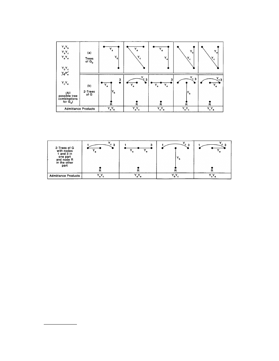
© 2000 by CRC Press LLC
the 2-trees in the gain expression by the k-tree approach correspond (one-to-one) to the uncanceled terms in
the final expressions of the gain by the flowgraph techniques. Finally, it should be obvious that the k-tree
approach depends upon the knowledge of the graph of a given network. Thus, if in a network problem only
the system of (loop or node) equations is given and the network is not known, or more generally, if a system
is characterized by a block diagram or a system of equations, the k-tree approach cannot be applied and one
must resort to the flowgraph techniques between the two approaches.
Some Topological Applications in Network Analysis and Design
In practice a circuit designer often has to make approximations and analyze the same network structure many
times with different sets of component values before the final network realization is obtained. Conventional
analysis techniques which require the evaluation of high-order determinants are undesirable even on a digital
computer because of the large amount of redundancy inherent in the determinant expansion process. The extra
calculation in the evaluation (expansion of determinants) and simplification (cancellation of terms) is time
consuming and costly and thereby contributes much to the undesirability of such methods.
The k-tree topological formulas presented in this section, on the other hand, eliminate completely the
cancellation of terms. Also, they are particularly suited for digital computation when the size of the network
is not exceedingly large. All of the terms involved in the formulas can be computed by means of a digital
compute using a single “tree-finding” program [Chan, 1969]. Thus, the application of topological formulas in
analyzing a network with the aid of a digital computer can mean a saving of a considerable amount of time
and cost to the circuit designer, especially true when it is necessary to repeat the same analysis procedure a
large number of times.
FIGURE 3.47
(a) The set of all trees of the modified graph G
3
, which corresponds to (b) the set of all 2-trees of G (with
nodes 3 and R in separate parts in each of such 2-tree).
FIGURE 3.48
The set of all 2-trees of G (with nodes l and 3 in one part of the reference node R in the other part of each
of such 2-tree).

© 2000 by CRC Press LLC
In a preliminary system design, the designer usually seeks one or more concepts which will meet the specifi-
cations, and in engineering practice each concept is generally subjected to some form of analysis. For linear
systems, the signal flowgraph of Mason is widely used in this activity. The flowgraph analysis is popular because
it depicts the relationships existing between system variables, and the graphical structure may be manipulated
using Mason’s formulas to obtain system transfer functions in symbolic or symbolic/numerical form.
Although the preliminary design problems are usually of limited size (several variables), hand derivation of
transfer functions is nonetheless difficult and often prone to error arising from the omission of terms. The
recent introduction of remote, time-shared computers into modern design areas offers a means to handle such
problems swiftly and effectively.
An efficient algorithm suitable for digital compution of transfer functions from the signal flowgraph descrip-
tion of a linear system has been developed (Dunn and Chan, 1969] which provides a powerful analytical tool
in the conceptual phases of linear system design.
In the past several decades, graph theory has been widely used in electrical engineering, computer science,
social science, and in the solution of economic problems [Swamy and Thulasiraman, 1981; Chen, 1990]. finally,
the application of graph theory in conjunction with symbolic network analysis and computer-aided simulation
of electronic circuits has been well recognized in recent years [Lin, 1991].
Defining Terms
Branches of a tree:
The edges contained in a tree.
Circuit (or loop):
A closed path where all vertices are of degree 2, thus having no endpoints in the path.
Circuit-set (or loop-set):
The set of all edges contained in a circuit (loop).
Connectedness:
A graph or subgraph is said to be connected if there is at least one path between every pair
of its vertices.
Flowgraph G
l
(or modified Coates graph G
l
):
The flowgraph G
l
(called the modified Coates graph) of a system
S of n independent linear equations in n unknowns
is an oriented graph such that the variable x
j
in S is represented by a node (also denoted by x
j
) in G
l
, and
the coefficient a
ij
of the variable x
j
in S by a branch with a branch gain a
ij
connected between nodes x
i
and x
j
in G
l
and directed from x
j
to x
i
. Furthermore, a source node l is included in G
l
such that for each
constant b
k
in S there is a node with gain b
k
in G
l
from node l to node s
k
. Graph G
ij
is the subgraph of
G
l
obtained by first removing all the outgoing branches from node x
j
and then short-circuiting node l
to node x
j
. A loop set l is a subgraph of G
l 0
that contains all the nodes of G
l 0
with each node having
exactly one incoming and one outgoing branch. The product p of the gains of all the branches in l is
called a loop-set product. A 2-loop-set l
2
is a subgraph of G
l j
containing all the nodes of G
l j
with each node
having exactly one incoming and one outgoing branch. The product p
2
of the gains of all the branches
in l
2
is called a 2-loop-set product.
k-tree admittance product of a k-tree:
The product of the admittances of all the branches of the k-tree.
k-tree of a connected graph G:
A proper subgraph of G consisting of k unconnected circuitless subgraphs,
each subgraph itself being connected, which together contain all the vertices of G.
Linear graph:
A set of line segments called edges and points called vertices, which are the endpoints of the
edges, interconnected in such a way that the edges are connected to (or incident with) the vertices. The
degree of a vertex of a graph is the number of edges incident with that vertex.
Path:
A subgraph having all vertices of degree 2 except for the two endpoints which are of degree 1 and are
called the terminals of the path, where the degree of a vertex is the number of edges connected to the
vertex in the subgraph.
Path-set:
The set of all edges in a path.
Proper subgraph:
A subgraph which does not contain all of the edges of the given graph.
a x
b
i
n
ij
j
n
j
i
=
å
=
=
1
1 2
, ,
,
. . .

© 2000 by CRC Press LLC
Signal-flowgraph G
m
(or Mason’s graph G
m
):
A signal-flowgraph G
m
of a system S of n independent linear
(algebraic) equations in n unknowns
is a graph with junction points called nodes which are connected by directed line segments called branches
with signals traveling along the branches only in the direction described by the arrows of the branches.
A signal x
k
traveling along a branch between x
k
and x
j
is multiplied by the gain of the branches g
kj
, so
that a signal g
kj
x
k
is delivered at node x
j
. An input node (source) is a node which contains only outgoing
branches; an output node (sink) is a node which has only incoming branches. A path is a continuous
unidirectional succession of branches, all of which are traveling in the same direction; a forward path is
a path from the input node to the output node along which all nodes are encountered exactly once; and
a feedback path (loop) is a closed path which originates from and terminates at the same node, and along
with all other nodes are encountered exactly once (the trivial case is a self-loop which contains exactly
one node and one branch). A path gain is the product of all the branch gains of the branches in a loop.
Subgraph:
A subset of the edges of a given graph.
Tree:
A connected subgraph of a given connected graph G which contains all the vertices of G but no circuits.
Related Topic
3.2 Node and Mesh Analysis
References
A.C. Aitken, Determinants and Matrices, 9th ed., New York: Interscience, 1956.
S.P. Chan, Introductory Topological Analysis of Electrical Networks, New York: Holt, Rinehart and Winston, 1969.
S.P. Chan and B.H. Bapna, “A modification of the Coates gain formula for the analysis of linear systems,” Inst.
J. Control, vol. 5, pp. 483–495, 1967.
S.P. Chan and S.G. Chan, “Modifications of topological formulas,” IEEE Trans. Circuit Theory, vol. CT-15,
pp. 84–86, 1968.
W.K. Chen, Theory of Nets: Flows in Networks, New York: Wiley Interscience, 1990.
C.L. Coates, “Flow-graph solutions of linear algebraic equations,” IRE Trans. Circuit Theory, vol. CT-6,
pp. 170–187, 1959.
W.R. Dunn, Jr., and S.P. Chan, “Flowgraph analysis of linear systems using remote timeshared computation,”
J. Franklin Inst., vol. 288, pp. 337–349, 1969.
G. Kirchhoff, “Über die Auflösung der Gleichungen, auf welche man bei der Untersuchung der linearen
Vertheilung galvanischer Ströme, geführt wird,” Ann. Physik Chemie, vol. 72, pp. 497–508, 1847; English
transl., IRE Trans. Circuit Theory, vol. CT-5, pp. 4–7, 1958.
P.M. Lin, Symbolic Network Analysis, New York: Elsevier, 1991.
S.J. Mason, “Feedback theory—Some properties of signal flow graphs,” Proc. IRE, vol. 41, pp. 1144–1156, 1953.
S.J. Mason, “Feedback theory—Further properties of signal flow graphs,” Proc. IRE, vol. 44, pp. 920–926, 1956.
J.C. Maxwell, Electricity and Magnetism, Oxford: Clarendon Press, 1892.
W.S. Percival, “Solution of passive electrical networks by means of mathematical trees,” Proc. IEE, vol. 100,
pp. 143–150, 1953.
S. Seshu and M.B. Reed, Linear Graphs and Electrical Networks, Reading, Mass.: Addison-Wesley, 1961.
M.N.S. Swamy ad K. Thulasiraman, Graphs, Networks, and Algorithms, New York: Wiley, 1981.
Further Information
All defining terms used in this section can be found in S.P. Chan, Introductory Topological Analysis of Electrical
Networks, Holt, Rinehart and Winston, New York, 1969. Also an excellent reference for the applications of graph
a x
b
i
n
ij
j
n
j
i
=
å
=
=
1
1 2
, ,
,
. . .
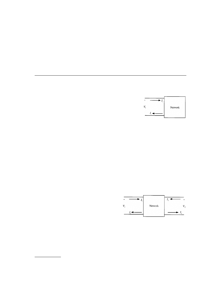
© 2000 by CRC Press LLC
theory in electrical engineering (i.e., network analysis and design) is S. Seshu and M.B. Reed, Linear Graphs
and Electrical Networks, Addison-Wesley, Reading, Mass., 1961.
For applications of graph theory in computer science, see M.N.S. Swamy and K. Thulasiraman, Graphs,
Networks, and Algorithms, Wiley, New York, 1981.
For flowgraph applications, see W.K. Chen, Theory of Nets: Flows in Networks, Wiley Interscience, New York,
1990.
For applications of graph theory in symbolic network analysis, see P.M. Lin, Symbolic Network Analysis,
Elsevier, New York, 1991.
3.7 Two-Port Parameters and Transformations
Norman S. Nise
Introduction
Many times we want to model the behavior of an electric network at only
two terminals as shown in
. Here, only V
1
and I
1
, not voltages and
currents internal to the circuit, need to be described. To produce the model
for a linear circuit, we use
to simplify the
network as viewed from the selected terminals. We define the pair of termi-
nals shown in Fig. 3.49 as a
, where the current, I
1
, entering one terminal
equals the current leaving the other terminal.
If we further restrict the network by stating that (1) all external connec-
tions to the circuit, such as sources and impedances, are made at the port
and (2) the network can have internal
, we can mathematically model the network at the port as
V
1
= ZI
1
(3.50)
or
I
1
= YV
1
(3.51)
where Z is the Thévenin impedance and Y is the Norton admittance at the terminals. Z and Y can be constant
resistive terms, Laplace transforms Z(s) or Y(s), or sinusoidal steady-state functions Z(j
w) or Y(jw).
Defining Two-Port Networks
Electrical networks can also be used to transfer signals from
one port to another. Under this requirement, connections to
the network are made in two places, the input and the output.
For example, a transistor has an input between the base and
emitter and an output between the collector and emitter. We
can model such circuits as
as shown in
. Here we see the input port, represented by V
1
and
I
1
, and the output port, represented by V
2
and I
2
. Currents
are assumed positive if they flow as shown in Fig. 3.50. The
same restrictions about external connections and internal sources mentioned above for the single port also apply.
Now that we have defined two-port networks, let us discuss how to create a mathematical model of the
network by establishing relationships among all of the input and output voltages and currents. Many possibilities
exist for modeling. In the next section we arbitrarily begin by introducing the z-parameter model to establish
the technique. In subsequent sections we present alternative models and draw relationships among them.
FIGURE 3.49
An electrical net-
work port.
FIGURE 3.50
A two-port network.

© 2000 by CRC Press LLC
Mathematical Modeling of Two-Port Networks via z Parameters
In order to produce a mathematical model of circuits represented by Fig. 3.50, we must find relationships
among V
1
, I
1
, V
2
, and I
2.
Let us visualize placing a current source at the input and a current source at the output.
Thus, we have selected two of the variables, I
1
and I
2
. We call these variables the independent variables. The
remaining variables, V
1
and V
2
, are dependent upon the selected applied currents. We call V
1
and V
2
the
dependent variables. Using
we can write each dependent variable as a function of the independent
variables as follows:
V
1
= z
11
I
1
+ z
12
I
2
(3.52a)
V
2
= z
21
I
1
+ z
22
I
2
(3.52b)
We call the coefficients, z
ij
, in Eqs. (3.52) parameters of the two-port network or, simply,
From Eqs. (3.52), the two-port parameters are evaluated as
(3.53)
Notice that each parameter can be measured by setting a port current, I
1
or I
2
, equal to zero. Since the parameters
are found by setting these currents equal to zero, this set of parameters is called
. Also,
since the definitions of the parameters as shown in Eqs. (3.53) are the ratio of voltages to currents, we
alternatively refer to them as
, or
. The parameters themselves can be
impedances represented as Laplace transforms, Z(s), sinusoidal steady-state impedance functions, Z(j
w), or
simply pure resistance values, R.
Evaluating Two-Port Network Characteristics in Terms of z Parameters
The two-port parameter model can be used to find the following characteristics of a two-port network when
used in some cases with a source and load as shown in
Input impedance = Z
in
= V
1
/I
1
(3.54a)
Output impedance = Z
out
= V
2
/I
2
| V
S
= 0 (3.54b)
Network voltage gain = V
g
= V
2
/V
1
(3.54c)
Total voltage gain = V
gt
= V
2
/V
S
(3.54d)
Network current gain = I
g
= I
2
/I
1
(3.54e)
To find Z
in
of Fig. 3.51, determine V
1
/I
1
. From Fig. 3.51, V
2
= –I
2
Z
L
. Substituting this value in Eq. 3.52(b)
and simplifying, Eqs. (3.52) become
(3.55a)
(3.55b)
z
V
I
z
V
I
z
V
I
z
V
I
I
I
I
I
11
1
1
0
12
1
2
0
21
2
1
0
22
2
2
0
2
1
2
1
=
=
=
=
=
=
=
=
;
;
V
z I
z I
1 11 1 12 2
=
+
0
21 1 22 2
=
+
+
( )
z I z Z I
L
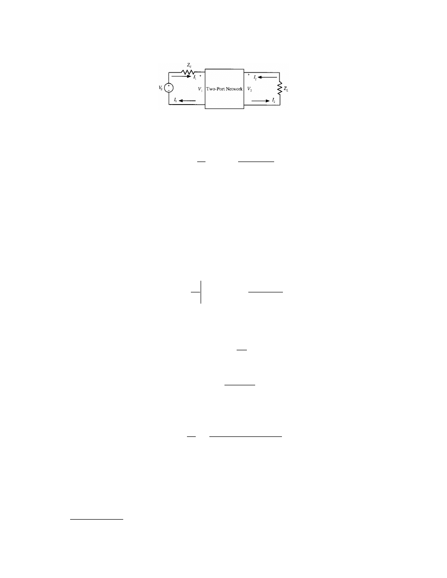
© 2000 by CRC Press LLC
Solving simultaneously for I
1
and then forming V
1
/I
1
= Z
in
, we obtain
(3.56)
To find Z
out
, set V
S
= 0 in Fig. 3.51. This step terminates the input with Z
S
. Next, determine V
2
/I
2
. From
Fig. 3.51 with V
S
shorted, V
1
= –I
1
Z
S
. By substituting this value into Eq. 3.52(a) and simplifying, Eqs. (3.52)
become
(3.57a)
(3.57b)
By solving simultaneously for I
2
and then forming V
2
/I
2
= Z
out
,
(3.58)
To find V
g
, we see from Fig. 3.51 that I
2
= –V
2
/Z
L
. Substituting this value in Eqs. (3.52) and simplifying, we
obtain
(3.59a)
(3.59b)
By solving simultaneously for V
2
and then forming V
2
/V
1
= V
g
,
(3.60)
Similarly, other characteristics, such as current gain and the total voltage gain from the source voltage to the
load voltage can be found.
summarizes many of the network characteristics that can be found using
z parameters as well as the process to arrive at the result.
FIGURE 3.51
Terminated two-port network for finding two-port network characteristics.
Z
V
I
z
z z
z
Z
L
in
=
=
-
+
( )
1
1
11
12 21
22
0
11 1 12 2
=
+
( )
+
z
Z I
z I
S
V
z I
z I
2 21 1 22 2
=
+
Z
V
I
z
z z
z
Z
Vs
S
out
=
=
-
+
( )
=
2
2
22
12 21
11
0
V
z I
z
Z
V
L
1
11 1
12
2
=
-
0
21 1
22
2
=
-
+
æ
è
ç
ö
ø
÷
z I
z
Z
Z
V
L
L
V
V
V
z Z
z
z
Z
z z
g
L
L
=
=
+
( )
-
2
1
21
11 22 12 21

© 2000 by CRC Press LLC
To summarize the process of finding network characteristics:
1. Define the network characteristic.
2. Use approproate relationships from Fig. 3.51.
3. Substitute the relationships from Step 2 into Eqs. (3.52).
4. Solve the modified equations for the network characteristic.
An Example Finding z Parameters and Network Characteristics
To solve for two-port network characteristics we can first represent the network with its two-port parameters
and then use these parameters to find the characteristics summarized in Table 3.1. To find the parameters, we
terminate the network adhering to the definition of the parameter we are evaluating. Then, we can use mesh
or nodal analysis, current or voltage division, or equivalent impedance to solve for the parameters. The following
example demonstates the technique.
Consider the network of
. The first step is to evaluate the z parameters. From their definition, z
11
and z
21
are found by open-circuiting the output and applying a voltage at the input as shown in
Thus, with I
2
= 0
(3.61a)
(3.61b)
TABLE 3.1
Network Characteristics Developed from z-Parameter Defining Eqs. (3.52)
Network
Characteristic Definition From Fig. 3.51
Substitute in Defining
Eqs. (3.52) and Obtain Solve for Network Characteristic
Input impedance
Output impedance
Network voltage gain
Total voltage gain
Network current gain
z
V
I
in
=
1
1
V
I Z
L
2
2
= -
V
z I
z I
z I z Z I
L
1 11 1 12 2
21 1 22 2
0
=
+
=
+
+
(
)
Z
z
z z
z
Z
L
in
=
-
+
11
12 21
22
Z
V
I
Vs
out
=
=
2
2 0
V
V
I Z
V
S
S
S
1
1
0
=
-
=
0
11 1 12 2
2 21 1 22 2
=
+
(
)
+
=
+
z
Z
I
z
I
V
z
I
z
I
S
Z
z
z z
z
Z
S
out
=
-
+
22
12 21
11
V
V
V
g
=
2
1
I
V
Z
L
2
2
= -
V
z I
z V
Z
z I
z
Z V
Z
L
L
L
1
11 1
12 2
21 1
22 2
0
=
-
=
-
+
(
)
V
z Z
z
z
Z
z z
g
L
L
=
+
(
)
-
21
11 22 12 21
V
V
V
S
gt
=
2
V
V
I Z
I
V
Z
S
S
L
1
1
2
2
=
-
= -
V
z
Z
I
z V
Z
z I
z
Z
V
Z
S
S
L
L
L
=
+
(
)
-
=
-
+
(
)
11 1
12 2
21 1
22 2
0
V
z Z
z
Z
z
Z
z z
L
S
L
gt
=
+
(
)
+
(
)
-
21
11 22 12 21
I
I
I
g
=
2
1
V
I Z
L
2
2
= -
V
z I
z I
z I z Z
I
L
1 11 1 12 2
21 1 22 2
0
=
+
=
+
+
(
)
I
z
z
Z
g
L
= -
+
21
22
6
4
1
1
I
I
V
a
-
=
-
+
=
4
18
0
1
I
I
a
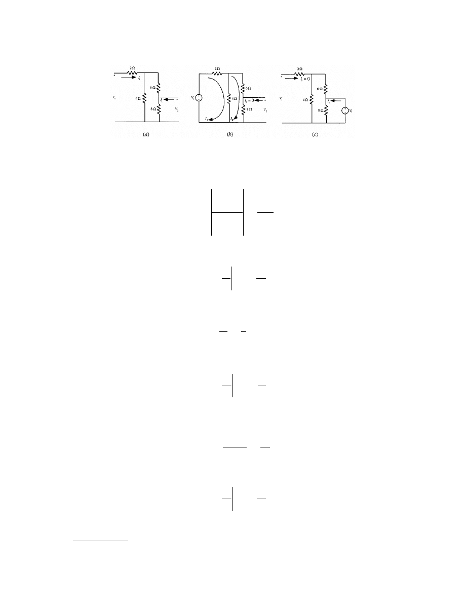
© 2000 by CRC Press LLC
Solving for I
1
yields
(3.62)
from which
(3.63)
We now find z
21
. From Eq. (3.61b)
(3.64)
But, from Fig. 3.52(b), I
a
= V
2
/8. Thus,
(3.65)
Based on their definitions, z
22
and z
12
are found by placing a source at the output and open-circuiting the
input as shown in
. The equivalent resistance, R
2eq
, as seen at the output with I
1
= 0 is
(3.66)
Therefore,
(3.67)
From Fig. 3.52(c), using voltage division
FIGURE 3.52
(a) Two-port network example; (b) two-port network modified to find z
11
and z
21
; (c) two-port network
modified to find z
22
and z
12
.
I
V
V
1
1
1
4
0
18
6
4
4
18
18
92
=
-
-
-
=
z
V
I
I
11
1
1 0
2
46
9
=
=
=
I
I
a
1
2
9
=
z
V
I
I
21
2
1 0
2
16
9
=
=
=
R
2
8
10
8
10
40
9
eq
=
´
+
=
z
V
I
I
22
2
2 0
1
40
9
=
=
=

© 2000 by CRC Press LLC
V
1
= (4/10)V
2
(3.68)
But
V
2
= I
2
R
2 e q
= I
2
(40/9) (3.69)
Substituting Eq. (3.69) into Eq. (3.68) and simplifying yields
(3.70)
Using the z-parameter values found in Eqs. (3.63), (3.65), (3.67), and (3.70) and substituting into the network
characteristic relationships shown in the last column of Table 3.1, assuming Z
S
= 20
W and Z
L
= 10
W, we
obtain Z
in
= 4.89
W, Z
out
= 4.32
W, V
g
= 0.252, V
gt
= 0.0494, and I
g
= –0.123.
Additional Two-Port Parameters and Conversions
We defined the z parameters by establishing I
1
and I
2
as the independent variables and V
1
and V
2
as the dependent
variables. Other choices of independent and dependent variables lead to definitions of alternative two-port
parameters. The total number of combinations one can make with the four variables, taking two at a time as
independent variables, is six.
defines the six possibilities as well as the names and symbols given to
the parameters.
The table also presents the expressions used to calculate directly the parameters of each set based upon their
definition as we did with z parameters. For example, consider the y, or
eters are seen to be
, since their evaluation requires V
1
or V
2
to be zero. Thus, to find
y
22
we short-circuit the input and find the admittance looking back from the output. For Fig. 3.52(a), y
22
=
23/88. Any parameter in Table 3.2 is found either by open-circuiting or short-circuiting a terminal and then
performing circuit analysis to find the defining ratio.
Another method of finding the parameters is to convert from one set to another. Using the “Definition” row
in Table 3.2, we can convert the defining equations of one set to the defining equations of another set. For
example, we have already found the z parameters. We can find the
as follows:
Solve for I
2
using the second z-parameter equation, Eq. (3.52b), and obtain the second h-parameter equation
as
(3.71)
which is of the form, I
2
= h
21
I
1
+ h
22
V
2
, the second h-parameter equation. Now, substitute Eq. (3.71) into the
first z-parameter equation, Eq. (3.52a), rearrange, and obtain
(3.72)
which is of the form, V
1
= h
11
I
1
+ h
12
V
2
, the first h-parameter equation. Thus, for example, h
21
= –z
21
/z
22
from
Eq. (3.71). Other transformations are found through similar manipulations and are summarized in Table 3.2.
Finally, there are other parameter sets that are defined differently from the standard sets covered here.
Specifically, they are scattering parameters used for microwave networks and image parameters used for filter
design. A detailed discussion of these parameters is beyond the scope of this section. The interested reader
should consult the bibliography in the “Further Information” section below, or Section 39.1 of this handbook.
z
V
I
I
12
1
2 0
1
16
9
=
=
=
I
z
z
I
z
V
2
21
22
1
22
2
1
= - +
V
z z z z
z
I
z
z
V
1
11 22 12 21
22
1
12
22
2
=
-
+
© 2000 by CRC Press LLC
TABLE 3.2
Two-Port Parameter Definitions and Conversions
Impedance Parameters
(Open-Circuit Parameters)
z
Admittance Parameters
(Short-Circuit Parameters)
y
Hybrid Parameters
h
Definition
Parameters
Conversion to z
parameters
Conversion to y
parameters
Conversion to h
parameters
Conversion to g
parameters
Conversion to T
parameters
Conversion to T
¢
parameters
D
V
z I
z I
V
z I
z I
1
11 1
12 2
2
21 1
22 2
=
+
=
+
I
y V
y V
I
y V
y V
1
11
1
12
2
2
21
1
22
2
=
+
=
+
V
h I
h V
I
h I
h V
1
11 1
12
2
2
21 1
22
2
=
+
=
+
z
V
I
z
V
I
z
V
I
z
V
I
I
I
I
I
11
1
1
0
12
1
2
0
21
2
1
0
22
2
2
0
2
1
2
1
=
=
=
=
=
=
=
=
;
;
y
I
V
y
I
V
y
I
V
y
I
V
V
V
V
V
11
1
1
0
12
1
1
0
21
2
1
0
22
2
1
0
2
1
2
1
=
=
=
=
=
=
=
=
;
;
h
V
I
h
V
V
h
I
I
h
I
V
V
I
V
I
11
1
1
0
12
1
2
0
21
2
1
0
22
2
2
0
2
1
2
1
=
=
=
=
=
=
=
=
;
;
z
y
z
y
z
y
z
y
y
y
y
y
11
22
12
12
21
21
22
11
=
=
-
=
-
=
D
D
D
D
;
;
z
h
z
h
h
z
h
h
z
h
h
11
22
12
12
22
21
21
22
22
22
1
=
=
=
-
=
D
;
;
y
z
y
z
y
z
y
z
z
z
z
z
11
22
12
12
21
21
22
11
=
=
-
=
-
=
D
D
D
D
;
;
y
h
y
h
h
y
h
h
y
h
h
11
11
12
12
11
21
21
11
22
11
1
=
=
-
=
=
;
;
D
h
z
h
z
z
h
z
z
h
z
z
11
22
12
12
22
21
21
22
22
22
1
=
=
=
-
=
D
;
;
h
y
h
y
y
h
y
y
h
y
y
11
11
12
12
11
21
21
11
22
11
1
=
=
-
=
=
;
;
D
g
z
g
z
z
g
z
z
g
z
z
11
11
12
12
11
21
21
11
22
11
1
=
=
-
=
=
;
;
D
g
y
g
y
y
g
y
y
g
y
y
11
22
12
12
22
21
21
22
22
22
1
=
=
=
-
=
D
;
;
g
h
g
h
g
h
g
h
h
h
h
h
11
22
12
12
21
21
22
11
=
=
-
=
-
=
D
D
D
D
;
;
A
z
z
B
z
C
z
D
z
z
z
=
=
=
=
11
21
21
21
22
21
1
;
;
D
A
y
y
B
y
C
y
D
y
y
y
=
-
=
-
=
-
=
-
22
21
21
21
11
21
1
;
;
D
A
h
B
h
h
C
h
h
D
h
h
=
-
=
-
=
-
=
-
D
21
11
21
22
21
21
1
;
;
¢ =
¢ =
¢ =
¢ =
A
z
z
B
z
C
z
D
z
z
z
22
12
12
12
11
12
1
;
;
D
¢ =
-
¢ =
-
¢ =
-
¢ =
-
A
y
y
B
y
C
y
D
y
y
y
11
12
12
12
22
12
1
;
;
D
¢ =
¢ =
¢ =
¢ =
A
h
B
h
h
C
h
h
D
h
h
1
12
11
12
22
12
12
;
;
D
D
z
z z
z z
=
-
11 22
12 21
D
y
y y
y y
=
-
11
22
12
21
D
h
h h
h h
=
-
11 22
12 21
© 2000 by CRC Press LLC
Inv. hybrid parameters
Transmission parameters
Inv. transmission par.
g
T
T’
Definition
Parameters
Conversion to z
parameters
Conversion to y
parameters
Conversion to h
parameters
Conversion to g
parameters
Conversion to T
parameters
Conversion to T
¢
parameters
D
Adapted from Van Valkenburg, M.E. 1974. Network Analysis, 3rd ed. Table 11-2, p. 337. Prentice-Hall, Englewood Cliffs, NJ.
With permission.
TABLE 3.2 (continued)
Two-Port Parameter Definitions and Conversions
I
g V
g I
V
g V
g I
1
11
1
12 2
2
21
1
22 2
=
+
=
+
V
AV
BI
I
CV
DI
1
2
2
1
2
2
=
-
=
-
V
A V
B I
I
C V
D I
2
1
1
2
1
1
=
¢
-
¢
=
¢
-
¢
g
I
V
g
I
I
g
V
V
g
V
I
I
V
I
V
11
1
1
0
12
1
2
0
21
2
1
0
22
2
2
0
2
1
2
1
=
=
=
=
=
=
=
=
;
;
A
V
V
B
V
I
C
I
V
D
I
I
I
V
I
V
=
=
-
=
=
-
=
=
=
=
1
2
0
1
2
0
1
2
0
1
2
0
2
2
2
2
;
;
¢ =
¢ =
-
¢ =
¢ =
-
=
=
=
=
A
V
V
B
V
I
C
I
V
D
I
I
I
V
I
V
2
1
0
2
1
0
2
1
0
2
1
0
1
1
1
1
;
;
z
g
z
g
g
z
g
g
z
g
g
11
11
12
12
11
21
21
11
22
11
1
=
=
-
=
=
;
;
D
z
A
C
z
C
z
C
z
D
C
T
11
12
21
22
1
=
=
=
=
;
;
D
z
D
C
z
C
z
C
z
A
C
T
11
12
21
22
1
=
¢
¢
=
¢
=
¢
=
¢
¢
¢
;
;
D
y
g
y
g
g
y
g
g
y
g
g
11
22
12
12
22
21
21
22
22
22
1
=
=
=
-
=
D
;
;
y
D
B
y
B
y
B
y
A
B
T
11
12
21
22
1
=
=
-
=
-
=
;
;
D
y
A
B
y
B
y
B
y
D
B
T
11
12
21
22
1
=
¢
¢
=
-
¢
=
-
¢
=
¢
¢
¢
;
;
D
h
g
h
g
h
g
h
g
g
g
g
g
11
22
12
12
21
21
22
11
=
=
-
=
-
=
D
D
D
D
;
;
h
B
D
h
D
h
D
h
C
D
T
11
12
21
22
1
=
=
=
-
=
;
;
D
h
B
A
h
A
h
A
h
C
A
T
11
12
21
22
1
=
¢
¢
=
¢
=
-
¢
=
¢
¢
¢
;
;
D
g
C
A
g
A
g
A
g
B
A
T
11
12
21
22
1
=
=
-
=
=
;
;
D
g
C
D
g
D
g
D
g
B
D
T
11
12
21
22
1
=
¢
¢
=
-
¢
=
¢
=
¢
¢
¢
;
;
D
A
g
B
g
g
C
g
g
D
g
g
=
=
=
=
1
21
22
21
11
21
21
;
;
D
A
D
B
B
C
C
D
A
T
T
T
T
=
¢
=
¢
=
¢
=
¢
¢
¢
¢
¢
D
D
D
D
;
;
¢ =
-
¢ =
-
¢ =
-
¢ =
-
A
g
B
g
g
C
g
g
D
g
g
D
12
22
12
11
12
12
1
;
;
¢ =
¢ =
¢ =
¢ =
A
D
B
B
C
C
D
A
T
T
T
T
D
D
D
D
;
;
D
g
g g
g g
=
-
11 22
12
21
D
T
AD
BC
=
-
D
¢
=
¢ ¢ -
¢ ¢
T
A D
B C

© 2000 by CRC Press LLC
Two-Port Parameter Selection
The choice of parameters to use for a particular analysis or design problem is based on analytical convenience
or the physics of the device or network at hand. For example, an ideal transformer cannot be represented with
z parameters. I
1
and I
2
are not linearly independent variables, since they are related through the turns ratio. A
similar argument applies to the
representation of a transformer. Here V
1
and V
2
are not indepen-
dent, since they too are related via the turns ratio. A possible choice for the transformer is the
. For an ideal transformer, B and C would be zero. For a BJT transistor, there is effectively linear
independence between the input current and the output voltage. Thus, the hybrid parameters are the parameters
of choice for the transistor.
The choice of parameters can be based also upon the ease of analysis. For example,
shows that “T”
networks lend themselves to easy evaluation of the z parameters, while y parameters can be easily evaluated for
“
P” networks. Table 3.3 summarizes other suggested uses and selections of network parameters for a few specific
cases. When electric circuits are interconnected, a judicious choice of parameters can simplify the calculations
to find the overall parameter description for the interconnected networks. For example, Table 3.3 shows that
the z parameters for series-connected networks are simply the sum of the z parameters of the individual circuits
(see Ruston et al., [1966] for derivations of the parameters for some of the interconnected networks). The bold
entries imply 2
´ 2 matrices containing the four parameters. For example,
(3.73)
Summary
In this section, we developed two-port parameter models for two-port electrical networks. The models define
interrelationships among the input and output voltages and currents. A total of six models exists, depending
upon which two variables are selected as independent variables. Any model can be used to find such network
characteristics as input and output impedance, and voltage and current gains. Once one model is found, other
models can be obtained from transformation equations. The choice of parameter set is based upon physical
reality and analytical convenience.
Defining Terms
Admittance parameters: That set of two-port parameters, such as y parameters, where all the parameters are
defined to be the ratio of current to voltage. See Table 3.2 for the specific definition.
Dependent source: A voltage or current source whose value is related to another voltage or current in the
network.
g Parameters:
See hybrid parameters.
h Parameters:
See hybrid parameters.
Hybrid (inverse hybrid) parameters:
That set of two-port parameters, such as h(g) parameters, where input
current (voltage) and output voltage (current) are the independent variables. The parenthetical expres-
sions refer to the inverse hybrid parameters. See Table 3.2 for specific definitions.
Impedance parameters: That set of two-port parameters, such as z parameters, where all the parameters are
defined to be the ratio of voltage to current. See Table 3.2 for the specific definition.
Independent source:
A voltage or current source whose value is not related to any other voltage or current
in the network.
Norton’s theorem:
At a pair of terminals a linear electrical network can be replaced with a current source in
parallel with an admittance. The current source is equal to the current that flows through the terminals
when the terminals are short-circuited. The admittance is equal to the admittance at the terminals with
all independent sources set equal to zero.
Open-circuit parameters: Two-port parameters, such as z parameters, evaluated by open-circuiting a port.
h
=
é
ë
ê
ù
û
ú
h
h
h
h
11 12
21 22
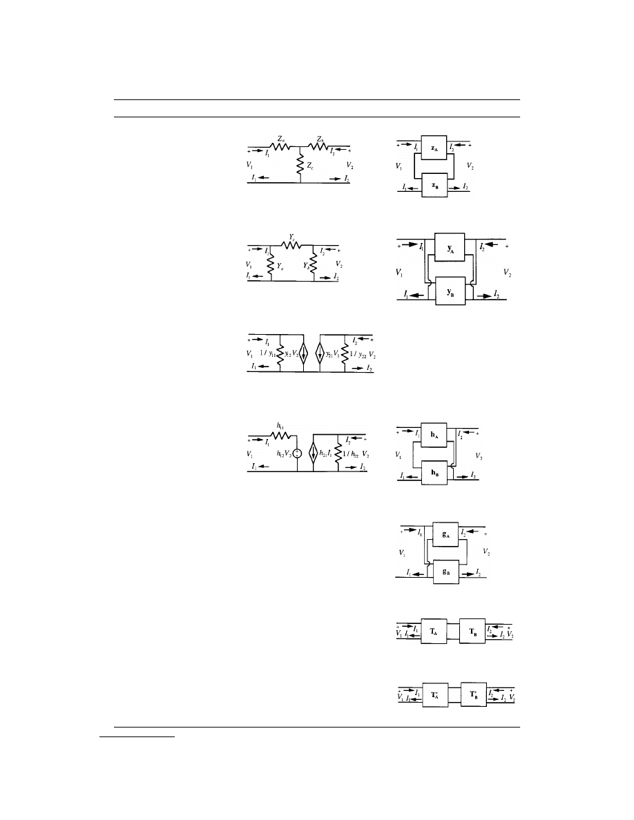
© 2000 by CRC Press LLC
TABLE 3.3
Two-Port Parameter Set Selection
Common Circuit Applications
Interconnected Network Applications
Impedance parameters z
• T networks
z
11
= Z
a
+ Z
e
;
z
12
= z
21
= Z
c
z
22
= Z
b
+ Z
c
• Series connected
z = z
A
+ z
B
Admittance parameters y
•
P networks
y
11
= Y
a
+ Y
c
;
y
12
= y
21
= –Y
c
y
22
= Y
b
+ Y
c
• Parallel connected
y = y
A
+ y
B
• Field effect transistor equivalent circuit
where typically:
1/y
11
=
¥, y
12
= 0, y
21
= g
m
, 1/y
22
= r
d
Hybrid parameters h
• Transistor equivalent circuit
where typically for common emitter:
h
11
= h
ie
, h
12
= h
re
, h
21
= h
fe
, h
22
= h
oe
• Series–parallel connected
h = h
A
+ h
B
Inverse hybrid parameters g
• Parallel-series connected
g = g
A
+ g
B
Transmission parameters T
• Ideal transformer circuits
• Cascade connected
T = T
A
T
B
Inverse transmission parameters T
¢
• Cascade connected
T
¢ = T¢
B
T
¢
A

© 2000 by CRC Press LLC
Port:
Two terminals of a network where the current entering one terminal equals the current leaving the
other terminal.
Short-circuit parameters:
Two-port parameters, such as y parameters, evaluated by short-circuiting a port.
Superposition:
In linear networks, a method of calculating the value of a dependent variable. First, the value
of the dependent variable produced by each independent variable acting alone is calculated. Then, these
values are summed to obtain the total value of the dependent variable.
Thévenin’s theorem:
At a pair of terminals a linear electrical network can be replaced with a voltage source
in series with an impedance. The voltage source is equal to the voltage at the terminals when the terminals
are open-circuited. The impedance is equal to the impedance at the terminals with all independent
sources set equal to zero.
T parameters:
See transmission parameters.
T
¢ parameters:
See transmission parameters.
Transmission (inverse transmission) parameters:
That set of two-port parameters, such as the T(T
¢) param-
eters, where the dependent variables are the input (output) variables of the network and the independent
variables are the output (input) variables. The parenthetical expressions refer to the inverse transmission
parameters. See Table 3.2 for specific definitions.
Two-port networks:
Networks that are modeled by specifying two ports, typically input and output ports.
Two-port parameters:
A set of four constants, Laplace transforms, or sinusoidal steady-state functions used
in the equations that describe a linear two-port network. Some examples are z, y, h, g, T, and T
¢ parameters.
y Parameters:
See admittance parameters.
z Parameters:
See impedance parameters.
Related Topic
3.3 Network Theorems
References
H. Ruston and J. Bordogna, “Two-port networks,” in Electric Networks: Functions, Filters, Analysis, New York:
McGraw-Hill, 1966, chap. 4, pp. 244–266.
M. E. Van Valkenburg, “Two-port parameters,” in Network Analysis, 3rd ed. Chap. 11, Englewood Cliffs, N.J.:
Prentice-Hall, 1974, pp. 325–350.
Further Information
The following texts cover standard two-port parameters:
J. W. Nilsson, “Two-port circuits,” in Electric Circuits, 4th ed., Reading Mass.: Addison-Wesley, 1995, chap. 21,
pp. 755–786.
H. Ruston and J. Bordogna, “Two-port networks,” in Electric Networks: Functions, Filters, Analysis, New York:
McGraw-Hill, 1966, chap. 4, pp. 206–311.
The following texts have added coverage of scattering and image parameters:
H. Ruston and J. Bordogna, “Two-port networks,” in Electric networks: Functions, Filters, Analysis, New York:
McGraw-Hill, 1966, chap. 4, pp. 266–297.
S. Seshu and N. Balabanian, “Two-port networks,” and “Image parameters and filter theory,” in Linear Network
Analysis, New York: Wiley, 1959, chaps. 8 and 11, pp. 291–342, 453–504.
The following texts show applications to electronic circuits:
F. H. Mitchell, Jr. and F. H. Mitchell, Sr., “Midrange AC amplifier design,” in Introduction to Electronics Design,
Englewood Cliffs, N.J.: Prentice-Hall, 1992, chap. 7, pp. 335–384.
C. J. Savant, Jr., M. S. Roden, and G. L. Carpenter, “Bipolar transistors,” “Design of bipolar junction transistor
amplifiers,” and “Field-effect transistor amplifiers,” in Electronic Design, 2nd ed., Redwood City, Calif.:
Benjamin/Cummings, 1991, chaps. 2, 3, and 4, pp. 69–212.
S. S. Sedra and K. C. Smith, “Frequency response” and “Feedback,” in Microelectronic Circuits, 3rd ed., Phila-
delphia, Pa.: Saunders, 1991, chaps. 7 and 8, pp. 488–645.
Document Outline
- Contents
- Linear Circuit Analysis
- 3.1Voltage and Current Laws
- 3.2Node and Mesh Analysis
- 3.3Network Theorems
- 3.4Power and Energy
- 3.5Three-Phase Circuits
- 3.6Graph Theory
- 3.7Two-Port Parameters and Transformations
Wyszukiwarka
Podobne podstrony:
78 Non Linear Circuits
77
circuit cellar1995 06
76 77
77 Nw 01 Wiertarka kolumnowa dok
77 Nw 01 Budujemy skiboby
circuit cellar1996 11
3S10 CIRCUIT ST92185
77 id 45963 Nieznany (2)
circuit cellar1995 12
76, 77
circuit cellar1996 04
circuit cellar1991 04,05
75 77
77 Impregnować czy nie impregnować
77
IV CR 216 77 id 220956 Nieznany
77 79
Phase Linear 200 II
więcej podobnych podstron