
Matrices, Mappings and
Crystallographic Symmetry
by
Hans Wondratschek
This electronic edition may be freely copied and
redistributed for educational or research purposes
only.
It may not be sold for profit nor incorporated in any product sold for profit without the
express permission of the Executive Secretary, International Union of Crystallography,
2 Abbey Square, Chester CH1 2HU, UK.
Copyright in this electronic edition c
2002 International Union of
Crystallography

Matrices, Mappings and Crystallographic
Symmetry
Hans Wondratschek
Institut f¨ur Kristallographie, Universit¨at Karlsruhe, Germany
Contents
Preface
3
List of symbols . . . . . . . . . . . . . . . . . . . . . . . . . . . . . .
4
Part I. Points, vectors and matrices
5
1
Points and vectors
5
1.1
Points and their coordinates . . . . . . . . . . . . . . . . . . . . .
5
1.2
Special coordinate systems: Cartesian coordinates . . . . . . . . .
7
1.3
Vectors
. . . . . . . . . . . . . . . . . . . . . . . . . . . . . . .
7
1.4
Vector coefficients . . . . . . . . . . . . . . . . . . . . . . . . . .
9
1.5
The scalar product and special bases . . . . . . . . . . . . . . . .
11
1.6
Distances and angles . . . . . . . . . . . . . . . . . . . . . . . .
14
2
Matrices and determinants
17
2.1
Mappings and symmetry operations . . . . . . . . . . . . . . . .
17
2.2
Motivation . . . . . . . . . . . . . . . . . . . . . . . . . . . . . .
19
2.3
The matrix formalism . . . . . . . . . . . . . . . . . . . . . . . .
21
2.4
Rules for matrix calculations . . . . . . . . . . . . . . . . . . . .
22
2.5
Determinants . . . . . . . . . . . . . . . . . . . . . . . . . . . .
25
2.6
Applications . . . . . . . . . . . . . . . . . . . . . . . . . . . . .
27
2.6.1
Inversion of a matrix . . . . . . . . . . . . . . . . . . . .
28
2.6.2
Distances and angles . . . . . . . . . . . . . . . . . . . .
29
2.6.3
The volume of the unit cell . . . . . . . . . . . . . . . . .
30

2
CONTENTS
Part II. Crystallographic applications
31
3
Crystallographic symmetry
31
3.1
Isometries . . . . . . . . . . . . . . . . . . . . . . . . . . . . . .
32
3.2
Crystallographic site–symmetry operations
. . . . . . . . . . . .
34
3.3
Space-group operations . . . . . . . . . . . . . . . . . . . . . . .
36
3.4
Crystallographic groups . . . . . . . . . . . . . . . . . . . . . . .
37
3.5
Display of crystallographic symmetry in IT A . . . . . . . . . . .
42
4
The description of mappings by ... pairs
46
4.1
Matrix–column pairs . . . . . . . . . . . . . . . . . . . . . . . .
46
4.2
Combination and reversion of mappings . . . . . . . . . . . . . .
47
4.3
(
4 × 4) matrices . . . . . . . . . . . . . . . . . . . . . . . . . . .
50
4.4
Transformation of vector coefficients . . . . . . . . . . . . . . . .
51
4.5
The matrix-column pairs of crystallographic symmetry operations
53
4.6
The ‘General Position’ in IT A . . . . . . . . . . . . . . . . . . .
55
5
Special aspects of the matrix formalism
59
5.1
Determination of the matrix-column pair . . . . . . . . . . . . . .
59
5.2
The geometric meaning of (W, w)
. . . . . . . . . . . . . . . . .
63
5.3
Coordinate transformations . . . . . . . . . . . . . . . . . . . . .
66
5.3.1
Origin shift . . . . . . . . . . . . . . . . . . . . . . . . .
66
5.3.2
Change of basis . . . . . . . . . . . . . . . . . . . . . . .
68
5.3.3
General coordinate transformations . . . . . . . . . . . .
69
6
Solution of the exercises
73
6.1
Solution of problem 1 . . . . . . . . . . . . . . . . . . . . . . . .
73
6.2
Solution of problem 2 . . . . . . . . . . . . . . . . . . . . . . . .
75
6.3
Solution of problem 3 . . . . . . . . . . . . . . . . . . . . . . . .
77
Index
79

3
Preface
This pamphlet is based on the manuscript for a summer school in Suez, Egypt, in
April 1997. Part I describes some elementary mathematics, similar to the manuscript
that was distributed to the school participants in advance of the school. It is in-
tended to remind the readers of selected mathematical concepts. Part II contains
the material that was covered in my six lectures and three exercise sessions at the
school. A carefully prepared Index is included for quick references.
In the analytical description of crystallographic symmetry, group theory is an in-
strument of utmost importance. Regrettably, there was no time to introduce group
theory during the school. The group-theoretical aspects of crystallography could
only be mentioned occasionally but not treated systematically. Therefore, also in
this pamphlet emphasis was put onto matrix methods. These are considered to be
more basic from the point of view of applications. The group–theoretical methods
can lead to a deeper insight into the crystallographic concepts and their relation-
ships later.
I very much enjoyed the interest of the participants and the stimulating discussions
with them and the other lecturers. The results of these discussions are taken into
account in this manuscript. I should like to thank in particular the chair of the
school, Karimat El–Sayed, as well as Farid Ahmed for their advice before, and
Jenny Glusker and Farid Ahmed for improving the final version of this article.
Brian McMahon has helped me with his technical expertise.

4
List of symbols
r, x, a, b, c, a
i
vectors
x, y, z, x
i
, r
i
, w
i
point coordinates, vector coefficients or coefficients of the
translation part of a mapping
x, r, w
column of point coordinates, of vector coefficients or of
the translation part of a mapping
˜
X,
˜x, ˜
x
i
image point, its column of coordinates and its coordinates
x
0
, x
0
i
column of coordinates and coordinates in a new coordinate
system
A
,
I
,
W
mappings
A,W, I
(3 × 3) matrices
A
ik
, B
ik
, W
ik
matrix coefficients
(A, a), (W, w)
matrix–column pairs
(a)
T
row of basis vectors
(a)
T
, (b)
T
, (r)
T
row of vector coefficients
A
T
transposed matrix
G, G
ik
fundamental matrix and its coefficients
a, b, c
lattice parameters
α, β, γ or α
j
angles between the basis vectors
Φ
angle between two vectors (bond angle)
det
(. . .)
determinant of a matrix
G, H, I, P, R, S
groups
W
,
x
,
˜
x
,
r
,
t
augmented matrix and columns
The International Tables for Crystallography, Vol. A (1983), 5th edition (2002),
will be abbreviated ‘IT A’.

5
Part I.
Points, vectors and matrices
1
Points and vectors
In this chapter, points and vectors are introduced. In spite of their strong rela-
tions, the difference between these concepts is emphasized. The distinction be-
tween them is sometimes not easy because both items are mostly described in the
same way, namely by columns of coefficients. Indeed, it is often not necessary
to know the real meaning of such columns, and they can be treated in the same
way independently of their nature. Sometimes, however, their behaviour is differ-
ent and their distinction is necessary for a real understanding of the description of
crystallographic objects and to avoid mistakes.
1.1
Points and their coordinates
A mathematical model of the space in which we live is the point space. Its ele-
ments are points. Objects in point space may be single points; finite sets of points,
e.g. the centres of the atoms of a molecule; infinite discontinuous point sets, e.g.
the centres of the atoms of an ideal (infinitely extended and periodic) crystal pat-
tern; continuous point sets like straight lines, curves, planes, curved surfaces, to
mention just a few which play a role in crystallography.
In the following we restrict our considerations to the 3-dimensional space. The
transfer to the plane should be obvious. One can even extend the whole concept to
n–dimensional space with arbitrary dimension n.
In order to describe the objects in point space analytically, one introduces a coor-
dinate system. To achieve this, one selects some point as the origin O. Then one
chooses three straight lines running through the origin and not lying in a plane.
They are called the coordinate axes a, b and c or a
1
, a
2
and a
3
. On each of these
lines a point different from O is chosen marking the unit on that axis: A on a, B
on b and C on c. An arbitrary point P is then described by its coordinates x, y, z
or x
1
, x
2
, x
3
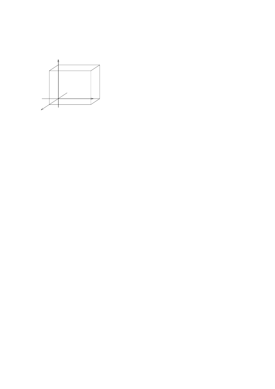
, see Fig. 1.1.1:
6
1
POINTS AND VECTORS
c
o
X
O
b
B
P
Z
C
Y
a
A
o
o
Fig. 1.1.1 Point P in a coordinate sys-
tem
{O, a, b, c}. The end points A, B
and C of the arrows determine the dif-
ferent unit lengths on the lines a, b and
c, respectively. The coordinate points
are X
◦
, Y
◦
and Z
◦
; the coordinates of
P are
x = (OX
◦
)/(OA),
y = (OY
◦
)/(OB) and
z = (OZ
◦
)/(OC).
Definition (D 1.1.1) The parallel coordinates x, y and z or x
1
, x
2
and x
3
of an
arbitrary point P are defined in the following way:
1. The origin O is the point with the coordinates 0, 0, 0.
2. One constructs the three planes through the point P which are parallel to
the pairs of axes b and c, c and a, and a and b, respectively. These three
planes intersect the coordinate axes a, b and c in the points X
◦
, Y
◦
and Z
◦
,
respectively.
3. The fractions of the lengths
(OX
◦
)/(OA) = x on the axis a,
(OY
◦
)/(OB) = y on b and (OZ
◦
)/(OC) = z on c are the coordinates of
the point P.
In this way one assigns uniquely to each point a triplet of coordinates and vice
versa. In crystallography the coordinates are written usually in a column which is
designated by a boldface–italics lower-case letter, e. g.,
P :
x
=
x
y
z
=
x
1
x
2
x
3
.
Definition (D 1.1.2) The set of all columns of three real numbers represents all
points of the point space and is called the affine space.
The affine space is not yet a good model for our physical space. In reality one can
measure distances and angles which is possible in the affine space only after the
introduction of a scalar product, see Sections 1.5 and 1.6. Such a space with a
scalar product is the fundament of the following considerations.
Definition (D 1.1.3) An affine space, for which a scalar product is defined, is
called a Euclidean space.
The coordinates of a point P depend on the position of P in space as well as on
the coordinate system. The coordinates of a fixed point P are changed by another
choice of the coordinate axes but also by another choice of the origin. Therefore,

1.2
Special coordinate systems: Cartesian coordinates
7
the comparison of two points by their columns of coordinates is only possible if
the coordinate system is the same to which these points are referred. Two points
are equal if and only if their columns of coordinates agree in all coordinates when
referred to the same coordinate system. If points are referred to different coordinate
systems and if the relations between these coordinate systems are known then one
can recalculate the coordinates of the points by a coordinate transformation in
order to refer them to the same coordinate system, see Subsection 5.3.3. Only after
this transformation a comparison of the coordinates is meaningful.
1.2
Special coordinate systems: Cartesian coordinates
There are different types of coordinate systems. Coordinate systems with straight
lines as axes as introduced in Section 1.1 are called parallel coordinates. In physics
polar coordinates in the plane and cylindrical or spherical coordinates in the space
are used frequently depending on the kind of problems.
In general those coordinates are chosen in which the solution of the given problem
is expected to cause the least difficulties. We shall consider mainly parallel coordi-
nates. Such coordinate systems are of utmost importance for crystallography due
to the periodicity of the crystals. In this section a special system with parallel coor-
dinates will be defined which is used frequently in physics, also in crystal physics
and in mathematics. It is applied in Section 1.6. In crystallography, mostly special
crystallographic coordinate systems are used.
Definition (D 1.2.1) A coordinate system with three coordinate axes perpendicular
to each other and lengths OA
= OB = OC = 1 is called a Cartesian coordinate
system.
Referring the points to a Cartesian coordinate system simplifies many formulae,
e. g. for the determination of distances between points and of angles between lines,
and thus makes such calculations particularly easy, cf. Sections 1.6 and 2.6. On the
other hand, the description of the symmetry of crystals, in particular of the trans-
lational symmetry (also in reciprocal space) becomes quite involved when using
Cartesian coordinates. With the exception of crystal physics, the disadvantages
of Cartesian coordinates outweigh their advantages when dealing with crystallo-
graphic problems.
1.3
Vectors
Vectors are objects which are encountered everywhere in crystallography: as dis-
tance vectors between atoms, as basis vectors of the coordinate system, as trans-
lation vectors of a crystal lattice, as vectors of the reciprocal lattice, etc. They are
elements of the vector space which is studied by linear algebra and is an abstract
space. However, vectors can be interpreted easily visually, see Fig. 1.3.1:

8
1
POINTS AND VECTORS
X
O
Y
Fig. 1.3.1 Vector
(
−→
XY ) from point X to
point Y. The vector represented by an ar-
row depends only on the relative but not on
the absolute sites of the points. The four
parallel arrows represent the same vector.
For each pair of points X and Y one can draw the arrow
−→
XY from X to Y. The
arrow
−→
XY is a representation of the vector r, as is any arrow of the direction and
length of r, see Fig. 1.3.1. The set of all vectors forms the vector space. The vector
space has no origin but instead there is the zero vector or o vector
(
−→
XX) which is
obtained by connecting any point X with itself. The vector r has a length which is
designed by
|r| = r, where r is a non–negative real number. This number is also
called the absolute value of the vector. A formula for the calculation of r can be
found in Sections 1.6 and 2.6.
For such vectors some simple rules hold which can be visualized, e. g. by a drawing
in the plane:
1. If λ is a real number then the vector λ
r = r λ is defined as the vector parallel
to r and with length
|λ r| = λ |r| = λ r.
In particular,
(1/r) r = r
◦
is a vector of length 1. Such a vector is called a
unit vector. Further
1 r = r; 0 r = o is the zero–vector with length 0. It is
the only vector with no direction.
(−1) r = −r is that vector which has the
same length as r,
|r| = |−r|, but opposite direction.
2. For successive multiplication with the real numbers λ and µ, the relation
µ (λ r) = (µ λ) r holds.
3. For two real numbers, λ and µ,
(λ + µ) r = λ r + µ r holds.
4. For two vectors, r and s, λ
(r + s) = λ r + λ s holds.
5. For two vectors, r and s,
r + s = s + r holds. This is called the commutative
law of vector addition, see Fig. 1.3.2 which is also called the parallelogram
of forces. In particular,
r + (−r) = r − r = o.
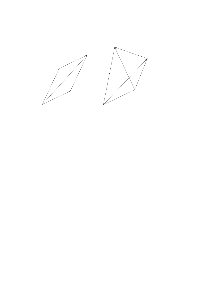
6. For any three vectors, r, s and t, the associative law of vector addition, see
Fig. 1.3.3,
(r + s) + t = r + (s + t) = r + s + t holds.
1.4
Vector coefficients
9
P
Q
r+s = s+r
R
r
S
r
s
s
Fig. 1.3.2 Visualization of the com-
mutative law of vector addition:
r
+ s = s + r.
P
s
T
s+t
t
S
R
r
r+s
r+s+t
Fig. 1.3.3 Visualization of the asso-
ciativity of vector addition:
(r + s) + t = r + (s + t).
Definition (D 1.3.1) A set of n vectors
r
1
,
r
2
, . . . ,
r
n
is called linearly independent
if the equation
λ
1
r
1
+ λ
2
r
2
+ . . . + λ
n
r
n
= 0
(1.3.1)
can only be fulfilled if λ
1
= λ
2
= . . . = λ
n
= 0. Otherwise, the vectors are called
linearly dependent.
In the plane any three vectors r
1
, r
2
and r
3
are linearly dependent because coeffi-
cients λ
i
can always be found such that λ
i
not all zero and
λ
1
r
1
+ λ
2
r
2
+ λ
3
r
3
= 0
holds.
Definition (D 1.3.2) The maximal number of linearly independent vectors in a
vector space is called the dimension of the space.
As is well known, the dimension of the plane is 2, of the space is 3. Any 4 vec-
tors in space are linearly dependent. Thus, if there are three linearly independent
vectors r
1
, r
2
and r
3
, then any other vector r can be represented in the form
r
= λ
1
r
1
+ λ
2
r
2
+ λ
3
r
3
.
Such a representation is widely used, it will be considered in the next section.
1.4
Vector coefficients
We start this section with a definition.
Definition (D 1.4.1) A set of three linearly independent vectors r
1
, r
2
and r
3
in
space is called a basis of the vector space. Any vector r of the vector space can be

10
1
POINTS AND VECTORS
written in the form r
= λ
1
r
1
+ λ
2
r
2
+ λ
3
r
3
. The vectors r
1
, r
2
and r
3
are called
basis vectors; the vector r is called a linear combination of r
1
, r
2
and r
3
. The real
numbers λ
1
, λ
2
and λ
3
are called the coefficients of r with respect to the basis r
1
,
r
2
, r
3
. In crystallography the two basis vectors for the plane are mostly called a
and b or
a
1
and
a
2
and the three basis vectors of the space are a, b and c or
a
1
,
a
2
and
a
3
.
The vector
−→
XY = r connects the points X and Y , see Fig. 1.3.1. In Section 1.1
the coordinates x, y and z of a point P have been introduced, see Fig. 1.1.1. We
now replace the section
(OA) on the coordinate axis a by the vector
−→
OA = a,
(OB) on b by
−→
OB = b, and (OC) on c by
−→
OC = c. If X and Y are given by
their columns of coordinates with respect to these coordinate axes, then the vector
(
−→
XY ) is determined by the column of the three coordinate differences between the
points X and Y . These differences are the vector coefficients of r:
r
=
y
1
− x
1
y
2
− x
2
y
3
− x
3
, where x =
x
1
x
2
x
3
and y =
y
1
y
2
y
3
.
(1.4.1)
As the point coordinates, the vector coefficients are written in a column. It is not
always obvious whether a column of three numbers represents a point by its coor-
dinates or a vector by its coefficients. One often calls this column itself a ‘vector’.
However, this terminology should be avoided. In crystallography both, points and
vectors are considered. Therefore, a careful distinction between both items is nec-
essary.
An essential difference between the behaviour of vectors and points is provided by
the changes in their coefficients and coordinates if another origin O
0
in point space
is chosen:
Let O
0
be the new, O the old origin, and o
0
the column of coordinates of O
0
with respect to the old coordinate system:
o
0
=
o
0
1
o
0
2
o
0
3
.
Then x
=
x
1
x
2
x
3
and y =
y
1
y
2
y
3
, the coordinates of X and Y in the old
coordinate system, are replaced by the columns x
0
=
x
0
1
x
0
2
x
0
3
and y
0
=
y
0
1
y
0
2
y
0
3
of the coordinates in the new coordinate system, see Fig. 1.4.1.
From
x = o
0
+ x
0
follows x
1
= o
0
1
+ x
0
1
and x
0
1
= x
1
− o
0
1
, etc. Therefore, the

1.5
The scalar product and special bases
11
coordinates of the points change if one chooses a new origin.
However, the coefficients of the vector
(
−→
XY ) do not change because of
y
0
1
− x
0
1
= y
1
− o
0
1
− (x
1
− o
0
1
) = y
1
− x
1
, etc.
......................
......................
.....................
......................
.....................
......................
.....................
......................
.....................
......................
.....................
......................
......................
.....................
......................
.....................
..............
................
....
....
..............
.............
..............
.............
..............
..............
.............
..............
..............
.............
..............
..............
.............
..............
.............
..............
..............
.............
..............
..............
.............
..............
..............
.............
.......
...........
.....
.....
...
...................................................................................................
....................................................................................................
.....................................................
................
....
....
...................
...................
...................
...................
...................
...................
...................
...................
...................
...................
..............
................
....
.... ........
..........
..........
..........
..........
..........
..........
..........
..........
..........
..........
..........
..........
..........
...
.........
.......
.......
.
o
0
O
.....
.....
.....
.....
.....
.....
.....
.....
.....
.....
.....
.....
.....
.....
.....
.....
.....
.....
.....
. .......
....
.............
r
y
Y
x
O
0
y
0
x
0
X
Fig. 1.4.1 The coordinates of the
points X and Y with respect to the
old origin O are x and y, with re-
spect to the new origin O
0
are x
0
and
y
0
. From the diagram one reads the
equations o
0
+ x
0
= x and
o
0
+ y
0
= y.
The rules 1., 2. and 5. of Section 1.3 (the others are then obvious) are expressed
by:
1. The vector x is multiplied with a real number λ
λ x = λ
x
1
x
2
x
3
=
λ x
1
λ x
2
λ x
3
.
2. For successive multiplication of x with λ and µ
µ(λ x) = µ
λ x
1
λ x
2
λ x
3
=
µ λ x
1
µ λ x
2
µ λ x
3
.
5. The sum
z = x + y of two vectors is calculated by their columns x and y
z
=
z
1
z
2
z
3
= x + y =
x
1
x
2
x
3
+
y
1
y
2
y
3
=
x
1
+ y
1
x
2
+ y
2
x
3
+ y
3
=
y
1
+ x
1
y
2
+ x
2
y
3
+ x
3
.
1.5
The scalar product and special bases
In order to express the angle between two vectors the scalar product is now intro-
duced. In this way also the bases can be characterized by their lattice parameters.
Definition (D 1.5.1) The scalar product (x , y) between two vectors x and y is
defined by
(x , y) =
|x| |y| cos (x, y).

12
1
POINTS AND VECTORS
For the scalar product the following rules hold:
1.
(x , y) = (y , x)
Commutative law
2. ((x + y) , z) = (x , z) + (y , z)
Distributive law
3.
(λ x , y) = λ (x , y) = (x , λ y).
(1.5.1)
Special cases.
(i) Because of cos 90
◦
= 0 the scalar product is zero if its vectors are perpen-
dicular to each other. Therefore, a scalar product may be zero even if none
of the vectors is the o vector.
(ii) If x = y, then because of cos 0
◦
= 1 the scalar product is the square of the
absolute value of x: (x, x) =
|x|
2
.
Two types of special bases shall be considered in this section.
The first one is the basis underlying the Cartesian coordinate system, see Section
1.2. It has the property that the scalar products between different basis vectors are
always zero:
(a
i
,
a
k
) = 0 for i, k = 1, 2, 3, i 6= k, because the basis vectors are
perpendicular to each other. In addition,
|a
i
| = 1 for any i because the basis vectors
have unit length. Such a basis is called an orthonormal basis. An orthonormal basis
allows simple calculations of distances and bonding angles, see the next section.
The other bases are those which are mostly used in crystallography. Real crystals in
the physical space may be idealized by crystal patterns which are 3–dimensional
periodic sets of points representing, e. g., the centres of the atoms of the crystal.
Because of the periodicity of the crystal pattern there are translations which map
the crystal pattern onto itself (often expressed by ‘the crystal pattern is left invari-
ant under the translation’). We consider these translations. If each of successive
translations leaves the crystal pattern invariant, then so does that translation which
results from the combination of the successive translations.
To each translation there belongs a translation vector. To the resulting translation
belongs that vector which is the sum of the vectors of the performed successive
translations. This means that for any set of translation vectors, all their integer
linear combinations are translation vectors of symmetry translations of the crystal
pattern as well.
Due to the finite size of the atoms the symmetry translations of a crystal pat-
tern cannot be arbitrarily short, there must be a minimum length (of a few ˚
A).
We choose three shortest translation vectors a
1
, a
2
and a
3
which do not lie in a
plane, i.e. which are linearly independent. Then any integer linear combination
v = v
1
a
1
+ v
2
a
2
+ v
3
a
3
, v
1
, v
2
, v
3
integer, of a
1
, a
2
and a
3
is a translation vector
of a symmetry translation as well. One can show that no other translation vector
may belong to a symmetry translation.
1.5
The scalar product and special bases
13
Definition (D 1.5.2) The set of all translation vectors belonging to symmetry
translations of a crystal pattern is called the vector lattice of the crystal pattern
(and of the real crystal). Its vectors are called lattice vectors. A basis of three lin-
early independent lattice vectors is called a lattice basis. If all lattice vectors are
integer linear combinations of the basis vectors, then the basis is called a primitive
lattice basis or a primitive basis.
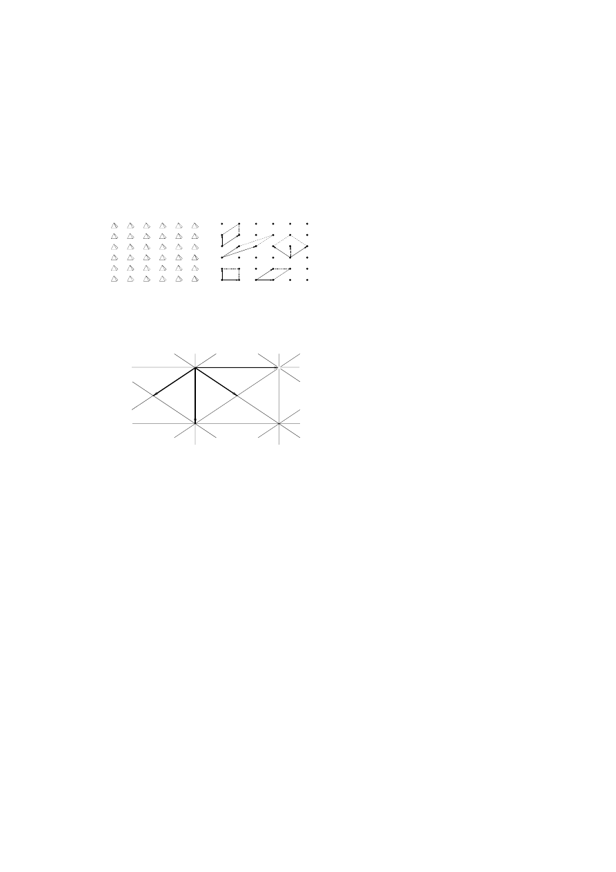
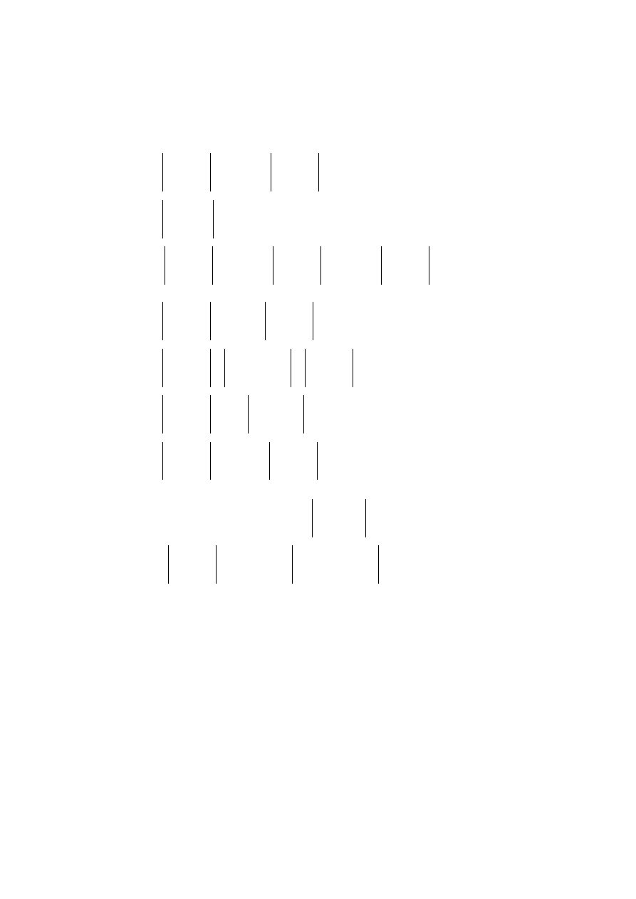
Fig. 1.5.1 Finite part of
a planar ‘crystal structure’
(left) with the correspond-
ing vector lattice (right). The
dots mark the end points of
the vectors.
Several bases are drawn in the right part of Fig. 1.5.1. Four of them are primitive,
among them the one which consists of the two shortest linearly independent lattice
vectors (lower left corner). The upper right basis is not primitive.
a’
a
b’
b
Fig. 1.5.2 c-centred lattice
(net) in the plane with con-
ventional a, b and primitive
a’, b’ bases.
Remarks.
1. If the vectors a
1
, a
2
and a
3
or a, b and c form a lattice basis, then any integer
linear combination of the basis vectors is a lattice vector as well. However,
there may be other vectors with rational non-integer coefficients which are
also lattice vectors. In this case crystallographers speak of a centred lattice
although not the lattice is centred but only the basis is chosen such that the
lattice appears to be centred.
Example, see Fig. 1.5.2. The lattice type c in the plane with conventional
basis a, b consists of all vectors v = n
1
a + n
2
b and v = (n
1
+ 1/2)a +
(n
2
+ 1/2)b, n
1
, n
2
integer. This basis is a lattice basis but not a primitive
one.
The basis a’ = a/2 – b/2, b’ = a/2 + b/2 would be a primitive basis. Referred
to this basis all lattice vectors have integer coefficients.
2. For any lattice a primitive basis may be chosen (for each lattice in the plane
or in the space there even exists an infinite number of primitive bases). The

14
1
POINTS AND VECTORS
basis chosen in IT A for the description of a lattice is called the conven-
tional basis. If the conventional basis is primitive, then also the lattice is
called primitive. For other reasons, the conventional basis is frequently
non–primitive such that the lattice appears to be centred. The conventional
centrings are c in the plane and C, A, B, I, F or R in the space.
3. In higher dimensions (dimension n >
3) the condition that the basis vectors
are shortest is no longer sufficient to guarantee a primitive basis.
Let a
i
be a basis. Then one can form the scalar products (a
i
, a
k
) between the basis
vectors, i, k = 1, 2, 3. Because (a
i
, a
k
) = (a
k
, a
i
), there are only six different scalar
products.
Definition (D 1.5.3) The quantities
a
1
= |a
1
| = +
p
(a
1
,
a
1
),
a
2
= |a
2
| = +
p
(a
2
,
a
2
),
a
3
= |a
3
| = +
p
(a
3
,
a
3
),
α
1
= arccos (|a
2
|
−1
|a
3
|
−1
(a
2
,
a
3
)),
α
2
= arccos (|a
3
|
−1
|a
1
|
−1
(a
3
,
a
1
)),
and α
3
= arccos (|a
1
|
−1
|a
2
|
−1
(a
1
,
a
2
))
are called the lattice parameters of the lattice.
The lengths of the basis vectors are mostly measured in ˚
A (1 ˚
A= 10
−10
m), some-
times in pm (1 pm = 10
−12
m) or nm (1 nm = 10
−9
m). The lattice parameters of a
crystal are given by its translations, more exactly, by the translation vectors of the
crystal pattern, they cannot be chosen arbitrarily. They may be further restricted
by the symmetry of the crystal.
Normally the conventional crystallographic bases are chosen when describing a
crystal structure. Referred to them the lattice of a crystal pattern may be primitive
or centred. If it is advantageous in exceptional cases to describe the crystal with
respect to another basis then this choice should be carefully stated in order to avoid
misunderstandings.
1.6
Distances and angles
When considering crystal structures, idealized as crystal patterns, frequently the
values of distances between the atoms (bond lengths) and of the angles between
atomic bonds (bonding angles) are wanted. These quantities cannot be calculated
from the coordinates of the points (centres of the atoms) directly. Distances and
angles are independent of the choice of the origin but the point coordinates depend
on the origin choice, see Section 1.4. Therefore, bond distances and angles can
only be calculated using the vectors (distance vectors) between the points partici-
pating in the bonding. In this section the necessary formulae for such calculations
will be derived.

1.6
Distances and angles
15
We assume the crystal structure to be given by the coordinates of the atoms (better:
of their centres) in a conventional coordinate system. Then the vectors between the
points can be calculated by the differences of the point coordinates.
Let
−→
XY = r = r
1
a
1
+ r
2
a
2
+ r
3
a
3
be the vector from point X to point Y ,
r
i
= y
i
− x
i
, see equation 1.4.1. The scalar product
(r , r) of r with itself is the
square of the length r of r. Thus
r
2
= (r , r) = ((r
1
a
1
+ r
2
a
2
+ r
3
a
3
) , (r
1
a
1
+ r
2
a
2
+ r
3
a
3
)).
Because of the rules for scalar products in equation (1.5.1), this can be written
r
2
= (r
1
a
1
, r
1
a
1
) + (r
2
a
2
, r
2
a
2
) + (r
3
a
3
, r
3
a
3
) +
2 (r
2
a
2
, r
3
a
3
) + 2 (r
3
a
3
, r
1
a
1
) + 2 (r
1
a
1
, r
2
a
2
).
It follows for the distance between the points X and Y
r
2
= r
2
1
a
2
1
+ r
2
2
a
2
2
+ r
2
3
a
2
3
+ 2 r
2
r
3
a
2
a
3
cos α
1
+
+ 2 r
3
r
1
a
3
a
1
cos α
2
+ 2 r
1
r
2
a
1
a
2
cos α
3
.
(1.6.1)
Using this equation, bond distances can be calculated if the coefficients of the bond
vector and the lattice parameters of the crystal are known.
The general formula (1.6.1) becomes much simpler for the higher symmetric crys-
tal systems. For example, referred to an orthonormal basis, equation (1.6.1) is re-
duced to
r
2
= r
2
1
+ r
2
2
+ r
2
3
.
(1.6.2)
16
1
POINTS AND VECTORS
Using the
Σ sign and abbreviating (a
i
,
a
k
) = G
ik
= a
i
a
k
cos α
j
(j is defined
for i
6= k: then k 6= j 6= i), the formula 1.6.1 can be written
r
2
=
3
X
i,k=1
G
ik
r
i
r
k
,
see also Subsection 2.6.2.
(1.6.3)
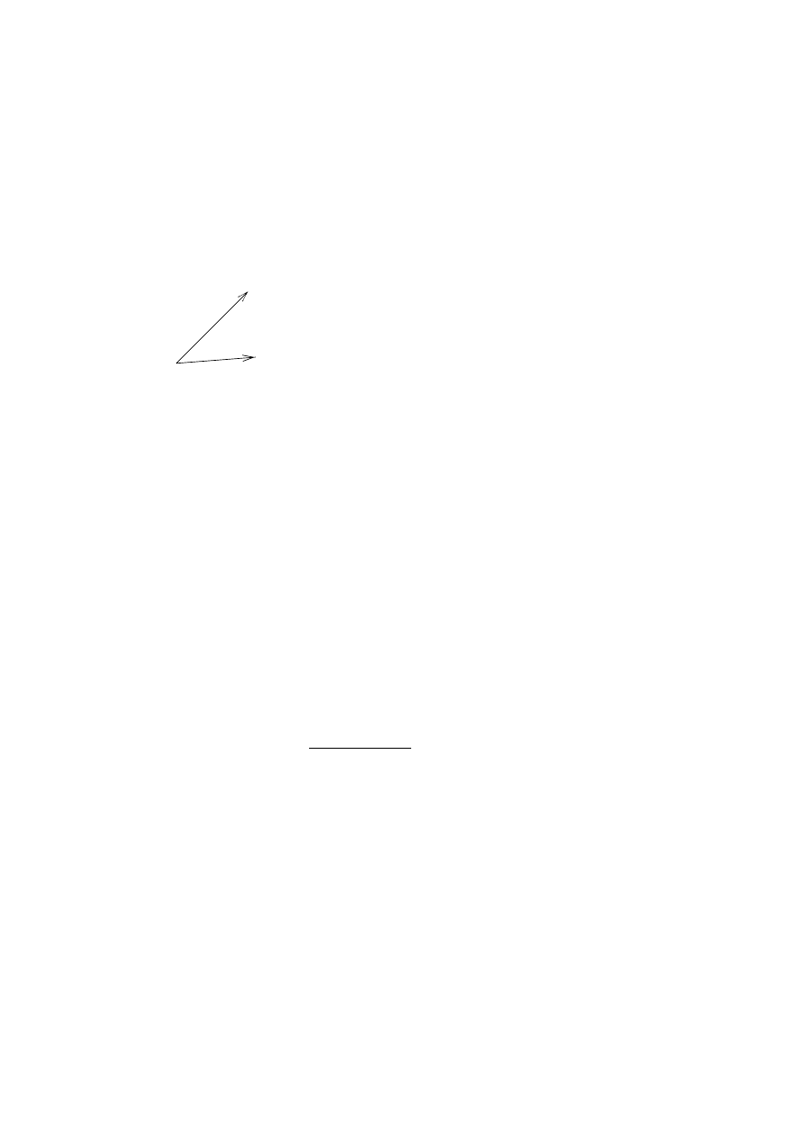
S
r
X
Φ
t
Y
Fig. 1.6.1 The bonding angle
Φ be-
tween the bond vectors
−→
SX = r and
−→
SY = t.
The (bonding) angle
Φ between the (bond) vectors
−→
SX = r and
−→
SY = t is calcu-
lated using the equation
(r , t) = |r| |t| cos Φ = r t cos Φ,
see Fig.
1.6.1.
One obtains
r t cos Φ = r
1
t
1
a
2
1
+ r
2
t
2
a
2
2
+ r
3
t
3
a
2
3
+ (r
2
t
3
+ r
3
t
2
) a
2
a
3
cos α
1
+
+ (r
3
t
1
+ r
1
t
3
) a
1
a
3
cos α
2
+ (r
1
t
2
+ r
2
t
1
) a
1
a
2
cos α
3
. (1.6.4)
Again one can use the coefficients G
ik
to obtain, see also Subsection 2.6.2,
cos Φ =
3
X
i,k=1
G
ik
r
i
r
k
−1/2
3
X
i,k=1
G
ik
t
i
t
k
−1/2
3
X
i,k=1
G
ik
r
i
t
k
.
(1.6.5)
For orthonormal bases, equation (1.6.4) is reduced to
r t cos Φ = r
1
t
1
+ r
2
t
2
+ r
3
t
3
,
(1.6.6)
and equation 1.6.5 is replaced by
cos Φ =
r
1
t
1
+ r
2
t
2
+ r
3
t
3
r t
.
(1.6.7)

17
2
Matrices and determinants
The second chapter deals with matrices and determinants which are essential for
the analytical description of crystallographic symmetry. Matrices are mathemat-
ical tools which may simplify involved calculations considerably and may make
complex formulae transparent. One can introduce them in an abstract way as a for-
malism and then apply them to many calculations in crystallography. However, it
seems to be better first to justify their introduction. Determinants are used for the
calculation of the volume, e. g. of a unit cell from the lattice parameters, or in the
process of inverting a matrix.
2.1
Mappings and symmetry operations
In crystallography, mapping an object of point space, e. g. the atomic centres of a
molecule or a crystal pattern, is one of the most basic procedures. Most crystal-
lographic mappings are rather special. Nevertheless, the term ‘mapping’ will be
introduced first in a more general way. What is a mapping of, e. g., a set of points ?
Definition (D 2.1.1) A mapping of a set A into a set B is a relation such that for
each element a
∈ A there is a unique element b ∈ B which is assigned to a. The
element b is called the image of a.
r
r
...........
............
..............
...............
............
..............
.............
...............
...................
..................................
.................................................................................................
.......................................................
..............
....
..
r
.........................................
..............................................
......................................................................................................................................................
..........................................
.......
................
....
˜
X1
X
˜
X2
Fig. 2.1.1 The relation of the point X to
the points ˜
X
1
and ˜
X
2
is not a mapping be-
cause the image point is not uniquely de-
fined (there are two image points).
1
3
2
4
5
Fig. 2.1.2 The five regions of the set A
(the triangle) are mapped onto the five
separated regions of the set B. No point
of A is mapped onto more than one im-
age point. Region 2 is mapped on a line,
the points of the line are the images of
more than one point of A. Such a map-
ping is called a projection.
The mapping which is displayed in Fig. 2.1.2 is rather complicated and can hardly
be described analytically. The mappings which are mainly used in crystallography
are much simpler: In general they map closed regions onto closed regions. Al-
though distances between points or angles between lines may be changed, parallel
lines of the original figure are always parallel also in the image. Such mappings are
called affine mappings. An affine mapping will in general distort an object, e. g.
by a shearing action or by an (isotropic or anisotropic) shrinking, see Fig. 2.1.3.
18
2
MATRICES AND DETERMINANTS
For example, in the space a cube may be distorted by an affine mapping into an
arbitrary parallelepiped but not into an octahedron or tetrahedron.
Fig. 2.1.3 In an affine mapping parallel
lines of the original figure (the rectan-
gular triangle) are mapped onto parallel
lines of the image (the nearly isoscale
triangle). Lengths and angles may be
distorted but relations of lengths on the
same line are preserved.
If an affine mapping leaves all distances and thus all angles invariant, it is called
isometric mapping, isometry, motion or rigid motion. We shall use the name ‘isom-
etry’. An isometry does not distort but moves the undistorted object through the
point space. However, it may change the orientation of an object, e. g. transfer a
right glove into an (otherwise identical) left one. Different types of isometries are
distinguished: In the space these are translations, rotations, inversions, reflections,
and the more complicated roto-inversions, screw rotations and glide reflections.
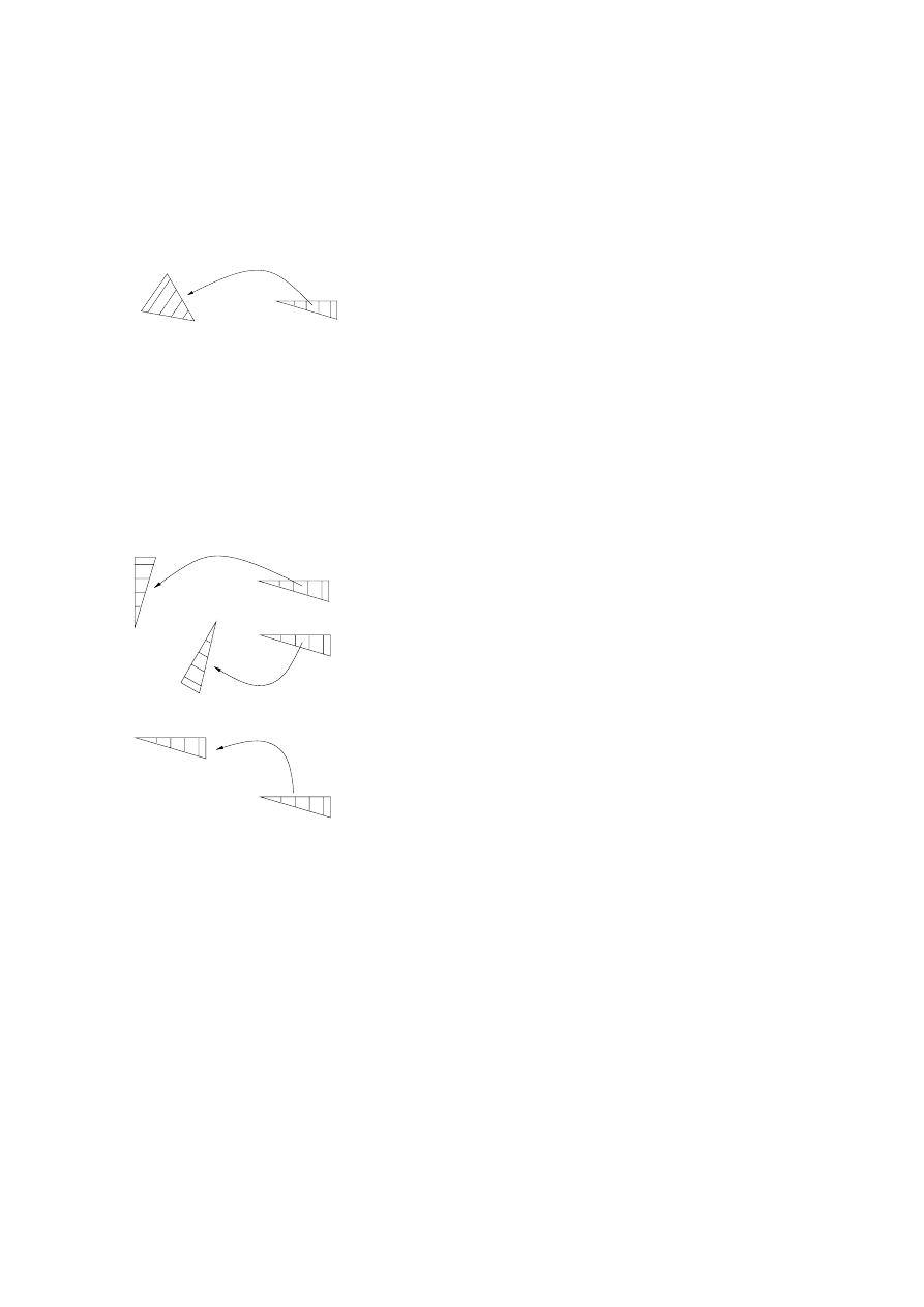
2
1
Fig. 2.1.4 An isometry leaves all distances
and angles invariant. An ‘isometry of the first
kind’, preserving the counter–clockwise se-
quence of the edges ‘short–middle–long’ of
the triangle is displayed in the upper mapping.
An ‘isometry of the second kind’, changing
the counter–clockwise sequence of the edges
of the triangle to a clockwise one is seen in the
lower mapping.
Fig. 2.1.5 A parallel shift of the triangle is
called a translation. Translations are spe-
cial isometries. They play a distinguished
role in crystallography.
One of the outstanding concepts in crystallography is ‘symmetry’. An object has
symmetry if there are isometries which map the object onto itself such that the
mapped object cannot be distinguished from the object in the original state. The
isometries which map the object onto itself are called symmetry operations of this
object. The symmetry of the object is the set of all its symmetry operations. If the
object is a crystal pattern, representing a real crystal, its symmetry operations are
called crystallographic symmetry operations.
2.2
Motivation
19
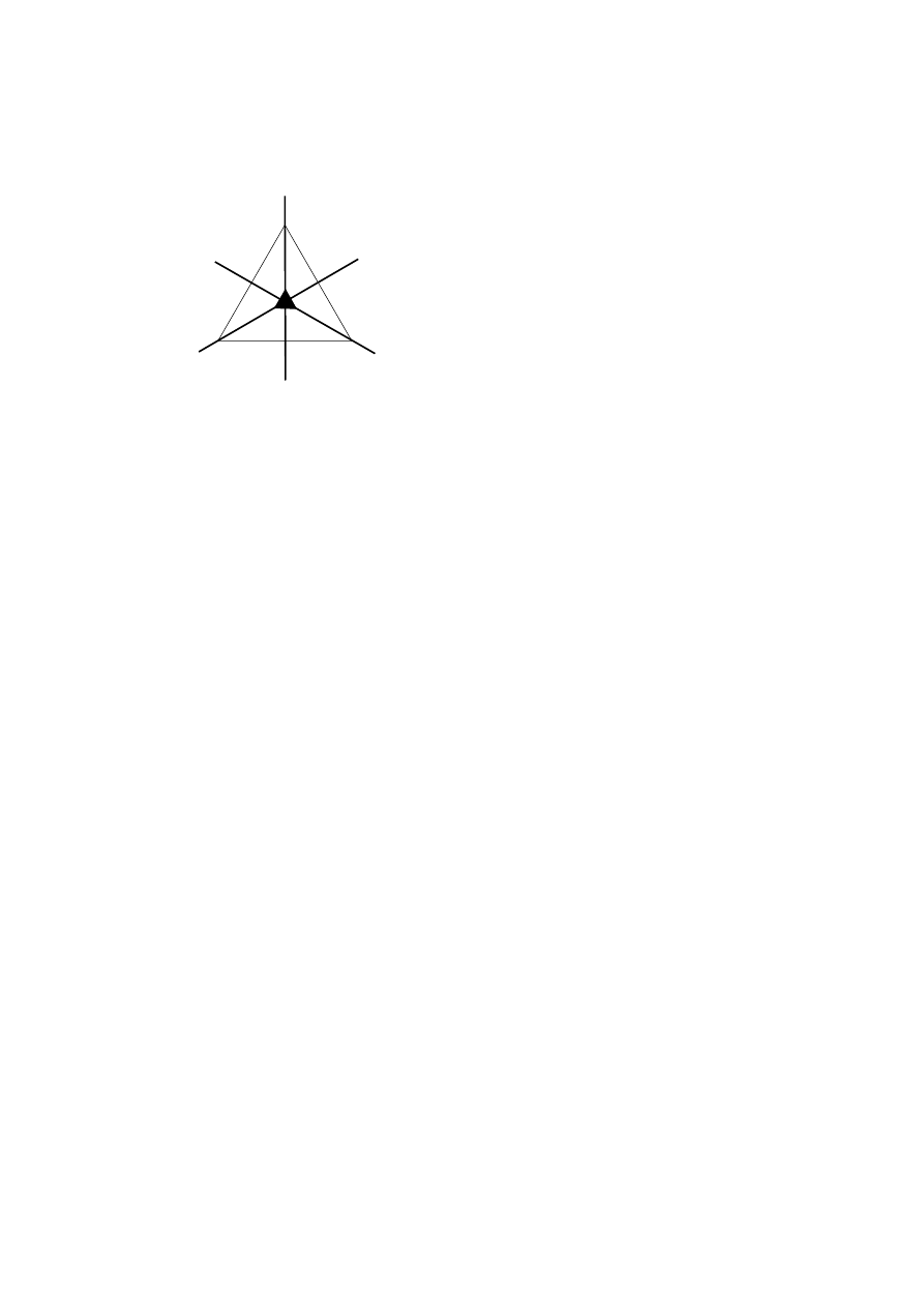
Fig. 2.1.6 The equilateral triangle
allows six symmetry operations: ro-
tations by
120
◦
and
240
◦
around its
centre, reflections through the three
thick lines intersecting the centre,
and the identity operation, see Sec-
tion 3.2.
2.2
Motivation
Any isometry may be the symmetry operation of some object, e. g. of the whole
space, because it maps the whole space onto itself. However, if the object is a
crystal pattern, due to its periodicity not every rotation, roto-inversion, etc. can be
a symmetry operation of this pattern. There are certain restrictions which are well
known and which are taught in the elementary courses of crystallography.
How can these symmetry operations be described analytically ? Having chosen a
coordinate system with a basis and an origin, each point of space can be repre-
sented by its column of coordinates. A mapping is then described by the instruc-
tion, in which way the coordinates
˜x of the image point ˜
X can be obtained from
the coordinates x of the original point X:
˜
x
1
= f
1
(x
1
, x
2
, x
3
), ˜
x
2
= f
2
(x
1
, x
2
, x
3
), ˜
x
3
= f
3
(x
1
, x
2
, x
3
).
The functions f
1
, f
2
andf
3
are not restricted for an arbitrary mapping. However,
for an affine mapping the functions f
i
are very simple: An affine mapping
X
−→ ˜
X is always represented in the form
˜
x
1
= A
11
x
1
+ A
12
x
2
+ A
13
x
3
+ a
1
˜
x
2
= A
21
x
1
+ A
22
x
2
+ A
23
x
3
+ a
2
.
˜
x
3
= A
31
x
1
+ A
32
x
2
+ A
33
x
3
+ a
3
(2.2.1)
A second mapping which brings the point ˜
X
−→ ˜˜
X is then represented by
˜˜x
1
= B
11
˜
x
1
+ B
12
˜
x
2
+ B
13
˜
x
3
+ b
1
˜˜x
2
= B
21
˜
x
1
+ B
22
˜
x
2
+ B
23
˜
x
3
+ b
2
˜˜x
3
= B
31
˜
x
1
+ B
32
˜
x
2
+ B
33
˜
x
3
+ b
3
,
or
(2.2.2)

20
2
MATRICES AND DETERMINANTS
˜˜x
1
=B
11
(A
11
x
1
+ A
12
x
2
+ A
13
x
3
+ a
1
) + B
12
(A
21
x
1
+ A
22
x
2
+ A
23
x
3
+ a
2
)
+ B
13
(A
31
x
1
+ A
32
x
2
+ A
33
x
3
+ a
3
) + b
1
;
˜˜x
2
=B
21
(A
11
x
1
+ A
12
x
2
+ A
13
x
3
+ a
1
) + B
22
(A
21
x
1
+ A
22
x
2
+ A
23
x
3
+ a
2
)
+ B
23
(A
31
x
1
+ A
32
x
2
+ A
33
x
3
+ a
3
) + b
2
;
˜˜x
3
=B
31
(A
11
x
1
+ A
12
x
2
+ A
13
x
3
+ a
1
) + B
32
(A
21
x
1
+ A
22
x
2
+ A
23
x
3
+ a
2
)
+ B
33
(A
31
x
1
+ A
32
x
2
+ A
33
x
3
+ a
3
) + b
3
.
(2.2.3)
The equations (2.2.3) may be rearranged in the following way:
˜˜x
1
= (B
11
A
11
+ B
12
A
21
+ B
13
A
31
)x
1
+ (B
11
A
12
+ B
12
A
22
+ B
13
A
32
)x
2
+ (B
11
A
13
+ B
12
A
23
+ B
13
A
33
)x
3
+ B
11
a
1
+ B
12
a
2
+ B
13
a
3
+ b
1
;
˜˜x
2
= (B
21
A
11
+ B
22
A
21
+ B
23
A
31
)x
1
+ (B
21
A
12
+ B
22
A
22
+ B
23
A
32
)x
2
+ (B
21
A
13
+ B
22
A
23
+ B
23
A
33
)x
3
+ B
21
a
1
+ B
22
a
2
+ B
23
a
3
+ b
2
;
˜˜x
3
= (B
31
A
11
+ B
32
A
21
+ B
33
A
31
)x
1
+ (B
31
A
12
+ B
32
A
22
+ B
33
A
32
)x
2
+ (B
31
A
13
+ B
32
A
23
+ B
33
A
33
)x
3
+ B
31
a
1
+ B
32
a
2
+ B
33
a
3
+ b
3
.
(2.2.4)
Although straightforward, one will agree that this is not a comfortable way to
describe and solve the problem of combining mappings. Matrix formalism does
nothing else than to formalize what is being done in equations (2.2.1) to (2.2.4),
and to describe this procedure in a kind of shorthand notation, called the matrix
notation:
Equation (2.2.1) is written
˜x = Ax + a;
(2.2.5)
Equation (2.2.2) is written ˜
˜x = B˜x + b;
(2.2.6)
Equation (2.2.3) is written ˜
˜x = B(Ax + a) + b;
(2.2.7)
Equation (2.2.4) is written ˜
˜x = BAx + Ba + b.
(2.2.8)
The matrix notation for mappings will be dealt with in more detail in Sections 4.1
and 4.2. In the next section the matrix formalism will be introduced.

2.3
The matrix formalism
21
2.3
The matrix formalism
Definition (D 2.3.1) A rectangular array of real numbers in m rows and n columns
is called a real (m
× n) matrix A:
A
=
A
11
A
12
. . .
A
1n
A
21
A
22
. . .
A
2n
..
.
..
.
. .
.
..
.
A
m1
A
m2
. . .
A
mn
.
The left index, running from 1 to m, is called the row index, the right index, running
from 1 to n, is the column index of the matrix. If the elements of the matrix are
rational numbers, the matrix is called a rational matrix; if the elements are integers
it is called an integer matrix.
Definition (D 2.3.2) An
(n × n) matrix is called a square matrix,
an
(m × 1) matrix a column matrix or just a column, and
a
(1 × n) matrix a row matrix or, for short, a row.
The index ‘1’ for column and row matrices is often omitted.
Definition (D 2.3.3) Let A be an
(m × n) matrix. The (n × m) matrix which is
obtained from A = (A
ik
) by exchanging rows and columns, i. e. the matrix (A
ki
),
is called the transposed matrix A
T
.
Example. If A
=
1 0 ¯1
2 4 ¯3
, then A
T
=
1 2
0 4
¯1 ¯3
.
(Crystallographers frequently write negative numbers
−z as ¯z, e. g. for M
ILLER
indices or elements of matrices).
Remark. In crystallography point coordinates or vector coefficients are written as
columns. In order to distinguish columns from rows (the M
ILLER
indices, e. g., are
written as rows), rows are regarded as transposed columns and are thus marked by
(..)
T
.
General matrices, including square matrices, will be designated by boldface-italics
upper case letters A, B, W, . . . ;
columns by boldface-italics lower case letters a, b, . . . and
rows by (a)
T
, (b)
T
, . . . , see also p. 4, List of symbols.
A square matrix A is called symmetric if A
T
= A, i. e. if A
ik
= A
ki
holds for any
pair i, k.
A symmetric matrix is called a diagonal matrix if A
ik
= 0 for i 6= k.
A diagonal matrix with all elements A
ii
= 1 is called the unit matrix I.
A matrix consisting of zeroes only, i. e. A
ik
= 0 for any pair i, k is called the
O–matrix.

22
2
MATRICES AND DETERMINANTS
We shall need only the special combinations m, n
= 3, 3 ‘square matrix’; m, n =
3, 1 ‘column matrix’ or ‘column’ , and m, n = 1, 3 ‘row matrix’ or ‘row’. How-
ever, the formalism does not depend on the sizes of m and n. Therefore, and be-
cause of other applications, formulae are displayed for general m and n. For ex-
ample, in the Least–Squares procedures of X-ray crystal–structure determination
huge (m
× n) matrices are handled.
2.4
Rules for matrix calculations
Matrices can be multiplied with a number or can be added, subtracted and multi-
plied with each other. These operations obey the following rules:
Definition (D 2.4.1) An
(m × n) matrix A is multiplied with a (real) number λ by
multiplying each element with λ:
A
=
A
11
A
12
. . . A
1n
A
21
A
22
. . . A
2n
..
.
..
.
. .
.
..
.
A
m1
A
m2
. . . A
mn
−→ λA =
λA
11
λA
12
. . . λA
1n
λA
21
λA
22
. . . λA
2n
..
.
..
.
. .
.
..
.
λA
m1
λA
m2
. . . λA
mn
.
Definition (D 2.4.2) Let A
ik
and B
ik
be the general elements of the matrices
A and B. Moreover, A and B must be of the same size, i. e. must have the same
number of rows and of columns. Then the sum and the difference A
± B is defined
by
C
= A ± B =
A
11
A
12
. . . A
1n
A
21
A
22
. . . A
2n
..
.
..
.
. .
.
..
.
A
m1
A
m2
. . . A
mn
±
B
11
B
12
. . . B
1n
B
21
B
22
. . . B
2n
..
.
..
.
. .
.
..
.
B
m1
B
m2
. . . B
mn
=
=
A
11
± B
11
A
12
± B
12
. . .
A
1n
± B
1n
A
21
± B
21
A
22
± B
22
. . .
A
2n
± B
2n
..
.
..
.
. .
.
..
.
A
m1
± B
m1
A
m2
± B
m2
. . .
A
mn
± B
mn
,
i. e. the element C
ik
of C is equal to the sum or difference of the elements A
ik
and
B
ik
of A and B for any pair of i, k: C
ik
= A
ik
± B
ik
.
The definition of matrix multiplication looks more complicated at first sight but
it corresponds exactly to what is written in full in the formulae (2.2.1) to (2.2.4)
of Section 2.2. The multiplication of two matrices is defined only if the number
n
(lema)
of columns of the left matrix is the same as the number m
(rima)
of rows
of the right matrix. The numbers m
(lema)
of rows of the left matrix and n
(rima)
of columns of the right matrix are free.

2.4
Rules for matrix calculations
23
We first define the product of a matrix A with a column a:
Definition (D 2.4.3) The multiplication of an (m
× n) matrix A with an (n × 1)
column a is only possible if the number n of columns of the matrix is the same
as the length of the column a. The result is the matrix product d = A a which is a
column of length m. The i-th element d
i
of d is
d
i
= A
i1
a
1
+ A
i2
a
2
+ . . . + A
ik
a
k
+ . . . + A
in
a
n
=
n
X
j=1
A
ij
a
j
.
(2.4.1)
For i
= 1, 2, 3 and n = 3 this is the same procedure as in equations (2.2.1) and
(2.2.2), where the coefficients x
k
in equation (2.2.1) and
˜
x
k
in equation (2.2.2) are
replaced by a
k
here, and the left sides
(˜
x
i
and ˜
˜
x
i
) are replaced by d
i
. The terms a
i
and b
i
of equations (2.2.1) and (2.2.2) are not represented in equation (2.4.1).
Written as a matrix equation this is
d
1
d
2
..
.
d
i
..
.
d
m
=
A
11
A
12
. . .
A
1k
. . .
A
1n
A
21
A
22
. . .
A
2k
. . .
A
2n
..
.
..
.
. .
.
..
.
..
.
A
i1
A
i2
. . .
A
ik
. . .
A
in
..
.
..
.
..
.
..
.
. .
.
..
.
A
m1
A
m2
. . .
A
mk
. . .
A
mn
a
1
a
2
..
.
a
k
..
.
a
n
.
In an analogous way one defines the multiplication of a row matrix with a general
matrix.
Definition (D 2.4.4) The multiplication of a
(1 × m) row a
T
, with an (m
× n)
matrix A is only possible if the length m, i. e. the number of ‘columns’, of the row
is the same as the number m of rows of the matrix. The result is the matrix product
d
T
= a
T
A which is a row of length n. The i-th element d
i
of d
T
is
d
i
= a
1
A
1i
+ a
2
A
2i
+ . . . + a
k
A
ki
+ . . . + a
m
A
mi
.
Written as a matrix equation this is
(d
1
d
2
. . . d
i
. . . d
n
) = (a
1
a
2
. . . a
k
. . . a
m
)
A
11
A
12
. . .A
1i
. . .A
1n
A
21
A
22
. . .A
2i
. . .A
2n
..
.
..
.
. .
.
..
.
..
.
A
k1
A
k2
. . .A
ki
. . .A
kn
..
.
..
.
..
.
. .
.
..
.
A
m1
A
m2
. . .A
mi
. . .A
mn
.

24
2
MATRICES AND DETERMINANTS
The multiplication of two matrices (both neither row nor column) is the combina-
tion of the already defined multiplications of a matrix with a column (matrix on
the left, column on the right side) or of a row with a matrix (row on the left, matrix
on the right side). Remember: The number of columns of the left matrix must be
the same as the number of rows of the right matrix.
Definition (D 2.4.5) The matrix product C = A B, or
C
11
C
12
. . .
C
1k
. . .
C
1n
C
21
C
22
. . .
C
2k
. . .
C
2n
..
.
..
.
. .
.
..
.
..
.
C
i1
C
i2
. . .
C
ik
. . .
C
in
..
.
..
.
..
.
. .
.
..
.
C
m1
C
m2
. . .
C
mk
. . .
C
mn
=
=
A
11
A
12
. . . A
1j
. . . A
1r
A
21
A
22
. . . A
2j
. . . A
2r
..
.
..
.
. .
.
..
.
..
.
A
i1
A
i2
. . . A
ij
. . . A
ir
..
.
..
.
..
.
. .
.
..
.
A
m1
A
m2
. . . A
mj
. . . A
mr
B
11
B
12
. . . B
1k
. . . B
1n
B
21
B
22
. . . B
2k
. . . B
2n
..
.
..
.
. .
.
..
.
..
.
B
j1
B
j2
. . . B
jk
. . . B
jn
..
.
..
.
..
.
. .
.
..
.
B
r1
B
r2
. . . B
rk
. . . B
rn
is defined by C
ik
= A
i 1
B
1k
+ A
i 2
B
2k
+ . . . + A
i j
B
jk
+ . . . + A
i r
B
rk
.
Examples.
If A
=
0 1 0
0 0 1
1 0 0
and B =
0 1 0
1 0 0
0 0 1
,
then C
= A B =
0 1 0
0 0 1
1 0 0
0 1 0
1 0 0
0 0 1
=
1 0 0
0 0 1
0 1 0
. On the
other hand, D
= B A =
0 1 0
1 0 0
0 0 1
0 1 0
0 0 1
1 0 0
=
0 0 1
0 1 0
1 0 0
.
Obviously, C
6=D, i. e. matrix multiplication is not always commutative. However,
it is associative, e. g., (A B) D = A (B D), as the reader may verify by performing
the indicated multiplications. One may also verify that matrix multiplication is
distributive, i. e.
(A + B) C = A C + B C.
In ‘indices notation’ (where A is an
(m×r) matrix, B an (r×n) matrix) the matrix

2.5
Determinants
25
product is
C
ik
=
r
X
j=1
A
ij
B
jk
, i = 1, . . . , m; k = 1, . . . , n.
(2.4.2)
Remarks.
1. The matrix A has the same number r of columns as B has rows; the number
m of rows is ‘inherited’ from A to C, the number n of columns from B to C.
2. A comparison with equation (2.2.4) shows that exactly the same construc-
tion occurs in the matrix product when describing consecutive mappings by
matrix–column pairs. Also the product of the matrix B with the column a
will be recognized. It is for this reason that the matrix formalism has been
introduced. Affine mappings (also isometries and crystallographic symme-
try operations) in point space are described by matrix–column pairs, see
Sections 2.2 and 4.1.
3. The ‘power notation’ is used in the same way for the matrix product of a
square matrix with itself as for numbers: A A = A
2
; A A A = A
3
, etc.
4. Using the formulae of this section one confirms equations (2.2.5) to (2.2.8).
2.5
Determinants
Matrices are frequently used when investigating the solutions of systems of linear
equations. Decisive for the solubility and the possible number of solutions of such
a system is a number, called the determinant
det(A) or |A| of A, which can be
calculated for any
(n × n) square matrix A. In this section determinants are intro-
duced and some of their laws are stated. Determinants are used to invert matrices
and to calculate the volume of a unit cell in Subsections 2.6.1 and 2.6.3.
The theory of determinants is well developed and can be treated in a very general
way. We only need determinants of (2
× 2) and (3 × 3) matrices and will discuss
only these.
Definition (D 2.5.1)
Let A
=
A
11
A
12
A
21
A
22
and B
=
B
11
B
12
B
13
B
21
B
22
B
23
B
31
B
32
B
33
be a
(2
× 2) and a (3 × 3) matrix. Then their determinants are designated by
det(A) =
A
11
A
12
A
21
A
22
anddet(B) =
B
11
B
12
B
13
B
21
B
22
B
23
B
31
B
32
B
33
and are defined by
the equations
det(A) = A
11
A
22
− A
12
A
21
and
(2.5.1)

26
2
MATRICES AND DETERMINANTS
det(B) = B
11
B
22
B
33
+ B
12
B
23
B
31
+ B
13
B
21
B
32
−
−B
11
B
23
B
32
− B
12
B
21
B
33
− B
13
B
22
B
31
.
(2.5.2)
Let D be a square matrix. If
det(D) 6= 0 then the matrix D is called regular, if
det(D) = 0, then D is called singular. Here only regular matrices are considered.
The matrix W of an isometry
W
is regular because always
det(W) = ±1. In
particular,
det(I) = +1 holds.
Remark. The determinant
det(A) is equal to the fraction ˜
V /V , where V is the vol-
ume of an original object and ˜
V the volume of this object mapped by the affine
mapping
A
. Isometries do not change distances, therefore they do not change vol-
umes and
det(W) = ±1 holds.
The following rules hold for determinants of
(n × n) matrices A. The columns of
A will be designated for these rules by A
k
, k = 1, . . . , n.
1.
det(A
T
) = det(A); the determinant of a matrix is the same as that of the
transposed matrix. Because of this rule the following rules, although formu-
lated only for columns, also hold if formulated for rows.
2. If one column of
det(A) is a multiple of another column, A
k
= λA
j
, then
det(A) = 0. This implies that det(A) = 0 if two columns of A are equal.
3. If a column A
k
is the sum of two columns B
k
and C
k
, A
k
= B
k
+ C
k
, then
det(A) = det(B) + det(C), where B is the matrix which has all columns of
A except that A
k
is replaced by B
k
, and C is the matrix with all columns of
A except that A
k
is replaced by C
k
.
4. Exchange of two columns, A
j
−→ A
k
and A
k
−→ A
j
of a determinant
changes its sign.
5. Adding to a column a multiple of another column does not change the value
of the determinant:
|A
1
A
2
. . . A
i
. . . A
k
. . . A
n
| = |A
1
A
2
. . . (A
i
+ λ A
k
) . . . A
k
. . . A
n
|.
6. Multiplication of all elements of a column with a number λ results in the
λ-fold value of the determinant:
|A
1
A
2
. . . λA
i
. . . A
k
. . . A
n
| = λ|A
1
A
2
. . . A
i
. . . A
k
. . . A
n
|.
7.
det(A B) = det(A) det(B), i. e. the determinant of a matrix product is equal
to the product of the determinants of the matrices.
8.
det(A
−1
) = (det(A))
−1
, for A
−1
see Subsection 2.6.1.
Among these rules there are three procedures which do not change the value of the
determinant:
(i) transposition;
(ii) an even number of exchanges of columns (or rows correspondingly), be-
cause
an odd number of exchanges changes the sign of the determinant; and
(iii) adding to a column a multiple of another column (or rows correspondingly).
2.6
Applications
27
Examples to the rules; calculation of the determinants according to equation (2.5.2).
1. A
=
1 1 3
2 2 2
3 2 3
= −4; A
T
=
1 2 3
1 2 2
3 2 3
= −4.
2. A
=
1 2 A
1 2 B
3 6 C
= 2C + 6B + 6A − 6B − 2C − 6A = 0.
3. A
=
1 1 3
2 2 2
3 2 3
= −4; B =
1 1 3
2 2 0
3 2 2
= −6; C =
1 1 0
2 2 2
3 2 1
= +2;
−4 = −6 + 2.
4. A
=
1 1 3
2 2 2
3 2 3
= −4; B =
1 3 1
2 2 2
3 3 2
= +4.
5. A
=
1 1 3
2 2 2
3 2 3
=
1 + 1 1 3
2 + 2 2 2
3 + 2 2 3
=
2 1 3
4 2 2
5 2 3
= −4.
6. A
=
1 1 3
2 2 2
3 2 3
= −4;
1 1 λ 3
2 2 λ 2
3 2 λ 3
= (−4) λ = −4 λ.
7. A
=
1 1 3
2 2 2
3 2 3
= −4; B =
¯1 0 4
1 2 1
0 1 3
= −1; (−4) (−1) = +4
is the product of the determinants.
The determinant of the product A B is
0 5 14
0 6 16
¯1 7 23
= +4.
8.
|A| =
1 1 3
2 2 2
3 2 3
= −4; |A
−1
| =
−1/2 −3/4 1
0
3/2 ¯1
1/2 −1/4 0
= −1/4.
2.6
Applications
Only a few applications can be dealt with here:
1. The inversion of a matrix;
2. Another formula for calculating the distance between points or the angle
between lines (bindings);
3. A formula for the volume of the unit cell of a crystal.

28
2
MATRICES AND DETERMINANTS
2.6.1
Inversion of a matrix
The inversion of a square matrix A is a task which occurs everywhere in matrix
calculations. Here we restrict the considerations to the inversion of (2
× 2) and
(3
× 3) matrices. In Least-Squares refiments the inversion of huge matrices was a
serious problem before the computers and programs were sufficiently developed.
Definition (D 2.6.1) A matrix C which fulfills the condition C A
= I for a given
matrix A, is called the inverse matrix or the inverse A
−1
of A.
The matrix A
−1
exists if and only if
det (A) 6= 0. In the following we assume C to
exist. If C A
= I then also A C = I holds, i. e. there is exactly one inverse matrix
of A. There are two possibilities to calculate the inverse matrix of a given matrix.
The first one is particularly simple but not always applicable. The other may be
rather tedious but always works.
Definition (D 2.6.2) A matrix A is called orthogonal if A
−1
= A
T
.
The name comes from the fact that the matrix part of any isometry is an orthogo-
nal matrix if referred to an orthonormal basis. In crystallography most matrices of
the crystallographic symmetry operations are orthogonal if referred to the conven-
tional basis.
Procedure: One forms the transposed matrix A
T
from the given matrix A and tests
if it obeys the equation A A
T
= I. If it does then the inverse A
−1
= A
T
is found.
If not one has to go the general way.
There are several general methods to invert a matrix. Here we use a formula based
on determinants. It is not restricted to dimensions 2 or 3.
Let A =
(A
ik
) be the matrix to be inverted, det(A) its determinant, and A
−1
=
((A
−1
)
ik
) be the inverted matrix which is to be determined. The coefficient
(A
−1
)
ik
is determined from the equation
(A
−1
)
ik
= (det(A))
−1
(−1)
i+k
B
ki
,
(2.6.1)
where B
ki
is that determinant which is obtained from
det(A) by canceling the k-th
row and i-th column. If
det(A) is a (2 × 2) determinant, then B
ki
is a number; if
det(A) is a (3 × 3) determinant, then B
ki
is a
(2 × 2) determinant. In general, if
det(A) is an (n × n) determinant, then B
ki
is an (
(n − 1) × (n − 1)) determinant.
Note that in this equation the indices of Bki are exchanged with respect to the
element
(A
−1
)ik which is to be determined.
Example.
Calculate the inverse matrix of A
=
1 2 0
¯1 0 3
2 ¯1 0
.
One determines
det(A) = 2·3·2−1·3·(−1) = 15 and obtains for the coefficients
of A
−1

2.6
Applications
29
(A
−1
)
11
= (−1)
2
0 3
¯1 0
/15 = 1/5; (A
−1
)
12
= (−1)
3
2 0
¯1 0
/15 = 0;
(A
−1
)
13
= (−1)
4
2 0
0 3
/15 = 2/5; (A
−1
)
21
= (−1)
3
¯1 3
2 0
/15 = 2/5;
(A
−1
)
22
= (−1)
4
1 0
2 0
/15 = 0;
(A
−1
)
23
= (−1)
5
1 0
¯1 3
/15 = −1/5;
(A
−1
)
31
= (−1)
4
¯1 0
2 ¯1
/15 = 1/15; (A
−1
)
32
= (−1)
5
1 2
2 ¯1
/15 = 1/3;
(A
−1
)
33
= (−1)
6
1 2
¯1 0
/15 = 2/15.
With these coefficients one finds A
−1
=
1/5
0
2/5
2/5
0 −1/5
1/15 1/3
2/15
and verifies that A A
−1
= A
−1
A
= I
holds.
2.6.2
Distances and angles
In Section 1.6 formulae for the distance between points (by calculating the
length of a vector) and the angle between bindings (vectors) have been derived.
The scalar products of the basis vectors have been designated by G
ik
, i, k
= 1, 2, 3.
They form the
fundamental matrix of the coordinate basis G
=
G
11
G
12
G
13
G
21
G
22
G
23
G
31
G
32
G
33
.
Because of G
ik
= G
ki
, G is a symmetric matrix.

30
2
MATRICES AND DETERMINANTS
In the formulae of Section 1.6 one may replace the ‘index formalism’ by the ‘ma-
trix formalism’. Using matrix multiplication with rows and columns,
one obtains the formula for the distance r
2
= r
T
G r,
with
G
=
a
2
1
a
1
a
2
cos γ
a
1
a
3
cos β
a
1
a
2
cos γ
a
2
2
a
2
a
3
cos α
a
1
a
3
cos β
a
2
a
3
cos α
a
2
3
.
(2.6.2)
This is the same as equation (1.6.3) but expressed in another way. Such ‘matrix
formulae’ are useful in general calculations when changing the basis, when de-
scribing the relation between crystal lattice and reciprocal lattice, etc. However,
for the actual calculation of distances, angles, etc. as well as for computer pro-
grams, the ‘index formulae’ of Section 1.6 are more appropriate.
For orthonormal bases, because of G = I equation (2.6.2) becomes very simple:
r
2
= r
T
r.
(2.6.3)
The formula for the angle
Φ between the vectors (
−→
SX) = r and (
−→
SY ) = t
is r t
cos Φ = r
T
G t, see Fig. 1.6.1,
or
cos Φ = (r
T
G r
)
−1/2
(t
T
G t
)
−1/2
r
T
G t.
(2.6.4)
2.6.3
The volume of the unit cell
The volume V of the unit cell of a crystal structure, i. e. the body containing all
points with coordinates
0 ≤ x
1
, x
2
, x
3
< 1, can be calculated by the formula
det(G) = V
2
.
(2.6.5)
In the general case one obtains
V
2
=
G
11
G
12
G
13
G
21
G
22
G
23
G
31
G
32
G
33
=
= a
2
b
2
c
2
(1 − cos
2
α
− cos
2
β
− cos
2
γ + 2 cos α cos β cos γ).
(2.6.6)
The formula (2.6.6) becomes simpler depending on the crystallographic symmetry,
i. e. on the crystal system.

31
Part II.
Crystallographic applications
The mathematical tools which have been developed in the first two chapters of
Part I will have useful applications here in Part II; since crystallographic studies
require both analytical treatment as well as geometric visualization. Geometric
models, perspective drawings, or projections of frames of symmetry, of crystal
structures and of complicated molecules are very instructive. However, often mod-
els are difficult to build, perspective drawings become confusing, and projections
suffer from loss of information. In addition, distances and angles may be distorted,
and it is sometimes not easy to see the important geometric relations.
Analytical methods, e. g. the matrix formalism, provide instruments which are of-
ten only slightly dependent on or even independent of the complexity of the sub-
ject. In many cases they can be applied using computers. Moreover, there are in-
ternal tests which enable the user to check the results of the calculations for inner
consistency. Such methods are indispensable in particular in crystal–structure de-
termination and evaluation. Only very simple crystal structures can be considered
without them.
Crystallographic symmetry and its applications have been investigated and de-
veloped by mineralogists, mathematicians, physicists and chemists from different
countries over several centuries. The result is the beautiful and still rapidly grow-
ing tree of contemporary crystallography. However, it is not necessary to know the
whole of this field of knowledge in order to apply and to take advantage of it. The
crystallographic tools necessary for the exploration of matter and for solid state
research can be taken from the volumes of the International Tables for Crystallog-
raphy series. Symmetry is described in Vol. A of this series. By the manuscript on
hand, the reader shall be enabled to use and exploit the contents of that volume A,
abbreviated IT A in this manuscript.
3
Crystallographic symmetry
In this chapter crystallographic symmetry will be outlined in a descriptive way. The
general concept of isometries is treated in Section 3.1. The restrictions imposed
on crystallographic symmetry operations are dealt with in Sections 3.2 for point–
group operations and 3.3 for space–group operations. The chapter is continued
with Section 3.4 on crystallographic groups and concluded by Section 3.5 where
the non–analytical description of crystallographic symmetry in IT A is dealt with.

32
3
CRYSTALLOGRAPHIC SYMMETRY
3.1
Isometries
An isometry
W
, see also Section 2.1,
1. maps each point P of the point space onto exactly one image point ˜
P:
˜
P =
W
P;
2. is a mapping of the point space onto itself which leaves all distances and
thus all angles invariant.
There are different types of isometries which will be characterized in this section.
For this characterization the notion of fixed points is essential.
Definition (D 3.1.1) Let
W
be an isometry and P a point of space. Then P is
called a fixed point of the isometry
W
if it is mapped onto itself (another term:
is left invariant) by
W
, i. e. if the image point ˜
P is equal to the original point P :
˜
P =
W
P = P .
The isometries are classified by their fixed points, and the fixed points are of-
ten used to characterize the isometries in visual geometric terms, see the follow-
ing types of isometries. Besides the ‘proper’ fixed points there are further objects
which are not fixed or left invariant pointwise but only as a whole. Lines and planes
of this kind are of great interest in crystallography, see the following examples.
Kinds of isometries.
The kinds 1. to 4. of isometries in the following list preserve the so–called ‘hand-
edness’ of the objects: if a right (left) glove is mapped by one of these isometries,
then the image is also a right (left) glove of equal size and shape. Such isometries
are also called isometries of the first kind or proper isometries. The kinds 5. to 8.
change the ‘handedness’: the image of a right glove is a left one, of a left glove is a
right one. These kinds of isometries are often called isometries of the second kind
or improper isometries.
1. Identity
I
. The identity mapping maps each point onto itself, each point of
space is a fixed point. All lines and planes of the space are left invariant as
well.
2. Translation
T
. By a translation each point of the point space is shifted in
the same direction by the same amount, such that the translation vector r
from each original point P to its image point ˜
P is independent of the point
P. There is no proper fixed point. Nevertheless, each line L parallel to r is
mapped onto itself as a whole, as is each plane which contains L. [The iden-
tity mapping may be considered as a special translation with r = o, where o
is the zero vector of length zero, see Section 1.3. Except if it is mentioned
explicitly, the term ‘translation’ is used for proper translations only, i. e. for
translations with
r 6= o.]
3. Rotation. Each rotation maps a line of points onto itself pointwise. This
line is called the rotation axis. The whole space is rotated around this axis

3.1
Isometries
33
by an angle
Φ, the rotation angle. The unit vector u
◦
parallel to the rotation
axis is called the direction of the rotation axis. Each plane perpendicular
to the rotation axis is mapped onto itself as a whole: it is rotated about the
intersection point of the plane with the rotation axis. For a 2–fold rotation
also each plane containing the rotation axis is left invariant as a whole. [The
identity operation may be considered as a special rotation with the rotation
angle
Φ = 0
◦
. Except if it is mentioned explicitly, the term ‘rotation’ is used
for proper rotations only, i. e. for rotations with
Φ 6= 0
◦
.]
4. Screw rotation. A screw rotation is a combination of a rotation (
u
◦
is the
direction of the rotation axis) and a translation with its translation vector
parallel to u
◦
. A screw rotation leaves no point fixed, the rotation axis of
the involved rotation is called the screw axis, and the vector of the involved
translation is the screw vector. The screw axis is not left fixed pointwise but
as a whole only (it is shifted parallel to itself by the involved translation). In
general the result of the combination of two isometries depends on the se-
quence in which the isometries are performed. The screw rotation, however,
is independent of the sequence of its two components.
5. Inversion. An inversion is the reflection of the whole space in a point P ,
which is called the centre of inversion. The point P is the only fixed point.
Each line or plane through P is mapped onto itself as a whole because it
is reflected in P . The inversion is an isometry of the second kind: any right
glove is mapped onto a left one and vice versa.
6. Rotoinversion. A rotoinversion can be understood as a combination of a
rotation with
Φ 6= 0
◦
and
Φ 6= 180
◦
and an inversion, where the centre of
inversion is placed on the rotation axis of the rotation. A rotoinversion is
an isometry of the second kind. The inversion point (which is no longer a
centre of inversion !) is the only fixed point; the axis of the rotation, now
called rotoinversion axis, is the only line mapped onto itself as a whole, and
the plane through the inversion point and perpendicular to the rotoinversion
axis is the only plane mapped onto itself as a whole. Again, a rotoinversion
does not depend on the sequence in which its components are performed.
7. Reflection. A reflection is another isometry of the second kind. Each point
of space is reflected in a plane, the reflection plane or mirror plane, such that
all points of this plane, and only these points, are fixed points. In addition,
each line and each plane perpendicular to the mirror plane is left invariant
as a whole.
8. Glide reflection. A glide reflection is an isometry of the second kind as well.
It can be conceived as a combination of a reflection in a plane and a trans-
lation parallel to this plane. The mirror plane of the reflection is now called
a glide plane. The translation vector of the translation involved is called the

34
3
CRYSTALLOGRAPHIC SYMMETRY
glide vector g. There is no fixed point of a glide reflection. Left invariant as
a whole are the glide plane and those planes which are perpendicular to the
glide plane and parallel to g as well as those lines of the glide plane which
are parallel to g.
Crystallographic symmetry operations may belong to any of these kinds of isome-
tries. They are designated in text and formulae by the so–called Hermann–Mauguin
symbols and in drawings by specific symbols which are all listed in IT A, Sec-
tion 1 as well as in the Brief Teaching Edition of Vol. A. Although each kind of
isometries is represented among the crystallographic symmetry operations, there
are restrictions which will be dealt with in the next two sections.
3.2
Crystallographic site–symmetry operations
In theoretical and practical work one frequently needs to know the symmetry
around a position in a molecule or in a crystal structure. The symmetry of the
surroundings of an atom or of the centre of gravity of a (more or less complex)
group of atoms (ion, molecule, etc.) is determined, among others, by chemical
bonds. The surroundings of such a constituent strongly influence the physical and
chemical properties of a substance. A striking example is the pair ‘graphite and
diamond’, which both are chemically carbon but display different surroundings of
the carbon atoms and thus extremely different chemical and physical properties.
The symmetry of the surroundings of a point P , called the site symmetry or point
symmetry of P , is determined by the symmetry of the whole molecule or crystal
and by the locus of P in the molecule or crystal. Here, we are interested in crys-
tallographic site symmetries only, i. e. the local symmetries around points P in a
crystal (better, in a crystal pattern). Strictly, one defines:
Definition (D 3.2.1) The set
R of all symmetry operations of a crystal pattern is
called the space group of the crystal pattern. The set of all elements of
R, i. e. of
the space group, which leave a given point P fixed, is called the site symmetry,
site–symmetry group, point–symmetry group, or point group
S of P with regard to
the space group
R.
In this manuscript the term site–symmetry group or, for short, site symmetry, is
preferred for reasons which will become clear in Section 3.4.
Because of its periodicity each crystal has an infinite number of translations as
symmetry operations, i. e.
R is an infinite set. However, a translation cannot be an
element of a site–symmetry group because a translation has no fixed point at all.
The same holds for screw rotations and glide reflections.
For the description of the crystallographic symmetry operations, it is convenient
to have available the notion of the ‘order of an isometry’.
Definition (D 3.2.2) An isometry
W
has the (or: is of) order k, if
W
k
= I holds,
where
I is the identity operation, and k > 0 is the smallest integer number for
which this equation is fulfilled.

3.2
Crystallographic site–symmetry operations
35
Remark. The k different isometries
W
j
, j = 1, . . . , k, form a group with k elements.
See also the definition (D 3.4.2) of the group order.
The following types of isometries may be elements of crystallographic site sym-
metries:
1. Identity. The identity
I
is a member of any crystallographic site–symmetry
group because it leaves any point fixed. It is the only operation whose order
is 1, its Hermann–Mauguin symbol (HM symbol) is also 1. [The HM sym-
bols have been introduced by C
ARL
H
ERMANN
and C
HARLES
M
AUGUIN
around 1930. There are HM symbols for point–group and for space–group
operations, as well as for site–symmetry, space and point groups. In IT A
the HM symbols form the standard nomenclature].
2. Inversion. If the inversion is a member of the site–symmetry group, then the
point P is the centre of inversion. The order of the inversion is 2, its HM
symbol is ¯
1.
3. Rotations. The point P is placed on the rotation axis. Due to the periodicity
of the crystals, the rotation angles of crystallographic rotations are restricted
to multiples of
60
◦
and
90
◦
, i. e. to
60
◦
,
120
◦
,
180
◦
,
240
◦
,
300
◦
,
90
◦
and
270
◦
. All these angles are of the form j
360
◦
/N , where N = 2, 3, 4 or 6, and
j is an integer which is relative prime to N . (This restriction does not hold
for the symmetry of molecules which may display, e. g., a rotation angle of
360
◦
/5 = 72
◦
and its multiples.) Moreover, the angles between different
axes of crystallographic rotations are limited to a small number of values
only.
A rotation with the rotation angle j
360
◦
/N is called an N –fold rotation. Its
HM symbol is N
j
. The HM symbols of the crystallographic rotations are
2
1
= 2
(180
◦
), 3
1
= 3
(120
◦
), 3
2
=
(240
◦
), 4
1
= 4
(90
◦
), 4
3
=
(270
◦
), 6
1
=
6 (60
◦
),
6
5
=
(300
◦
), (and 1 (0
◦
or
360
◦
) for the identity). The order of the rotation
N
j
is k
= N .
4. Rotoinversions. The point P is placed in the inversion point on the rotoin-
version axis. The restrictions on the angles
Φ of the rotational parts are the
same as for rotations. If
Φ = j 360
◦
/N , the rotoinversion is called an N –
fold rotoinversion. The HM symbol for such a rotoinversion is ¯
N
j
. In crys-
tals can occur:
(¯
1 inversion), ¯3
1
= ¯3, ¯3
5
, ¯
4
1
= ¯4, ¯4
3
, ¯
6
1
= ¯6 and ¯6
5
. The rotoinversion ¯
2 is
identical with a reflection, see next item.
Question
. Which isometry is ¯
3
3
, ¯
4
2
, ¯
6
2
and ¯
6
3
? The answer to this ques-
tion is found at the end of this chapter.
5. Reflections. The point P is situated on the mirror plane. There are only a few
possible angles between the normals of different mirror planes belonging to

36
3
CRYSTALLOGRAPHIC SYMMETRY
the reflections of a site–symmetry group:
30
◦
,
45
◦
,
60
◦
and
90
◦
. The HM
symbol of a reflection is m (mirror, miroir) instead of ¯
2. The order of a
reflection is 2, because its 2–fold application yields the identity operation.
The combination of these types of symmetry operations to site-symmetry or point
groups will be discussed in Section 3.4.
3.3
Space-group operations
The following facts are stated, their proof is beyond the scope of this manuscript:
1. The symmetry operations listed in Section 3.2 are elements of space groups
which leave the given point P fixed, see definition (D 3.2.1). Therefore,
identity, inversion, rotations, rotoinversions, and reflections are symmetry
operations of space groups. Moreover, the same restrictions for the possible
angles of rotation and rotoinversion of space–group operations hold as in
Section 3.2. This concerns also the rotations involved in screw rotations.
2. It is always possible to choose a primitive basis, see definition (D 1.5.2)
and the remarks to it. Referred to a primitive basis, all lattice vectors of the
crystal are integer linear combinations of the basis vectors. Each of these
lattice vectors defines a (symmetry) translation. The order of any translation
T
is infinite because there is no integer number k
6= 0 such that T
k
= I.
3. Parallel to each rotation, screw–rotation or rotoinversion axis as well as par-
allel to the normal of each mirror or glide plane there is a row of lattice
vectors.
4. Perpendicular to each rotation, screw–rotation, or rotoinversion axis as well
as parallel to each mirror or glide plane there is a plane of lattice vectors.
5. Let
Φ = 360
◦
/N be the rotation angle of a screw rotation, then the screw
rotation is called N –fold. Note that the order of any screw rotation is infinite.
Let u be the shortest lattice vector in the direction of the corresponding screw
axis, and n
u/N, with n 6= 0 and integer, be the screw vector of the screw
rotation by the angle
Φ. Then the HM symbol of the screw rotation is N
n
.
Performing an N –fold rotation N –times results in the identity mapping, i. e.
the crystal has returned to its original position. After N screw rotations with
rotation angle
Φ = 360
◦
/N the crystal has its original orientation but is
shifted parallel to the screw axis by the lattice vector n u.
6. Let
W
be a glide reflection. Then the glide vector is parallel to the glide plane
and is 1/2 of a lattice vector t. Whereas twice the application of a reflection
restores the original position of the crystal, applying a glide reflection twice
results in a translation of the crystal with the translation vector t. The order
of any glide reflection is infinite. The HM symbol of a glide reflection is

3.4
Crystallographic groups
37
g in the plane and a, b, c, d, e or n in the space. The letter indicates the
direction of the glide vector g relative to the basis of the coordinate system.
3.4
Crystallographic groups
The symmetry, i. e. the set of all symmetry operations, of any object forms a group
in the mathematical sense of the word. Therefore, the theorems and results of group
theory can be used when dealing with the symmetries of crystals. The methods of
group theory cannot be treated here but a few results of group theory for crystallo-
graphic groups will be stated and used.
We start with the definition of the terms ‘subgroup’ and ‘order of a group’.
Definition (D 3.4.1) Let
G and H be groups such that all elements of H are also
elements of
G. Then H is called a subgroup of G.
Remark. According to its definition, each crystallographic site–symmetry group is
a subgroup of that space group from which its elements are selected.
Definition (D 3.4.2) The number g of elements of a group
G is called the order of
G. In case g exists, G is called a finite group. If there is no (finite) number g, G is
called an infinite group.
Remark. The term ‘order’ is an old mathematical term and has nothing to do with
order or disorder in crystals. Space groups are always infinite groups; crystallo-
graphic site–symmetry groups are always finite.
The following results for crystallographic site–symmetry groups
S and point groups
P are known for more than 170, those for space groups R more than 100 years.
We consider site–symmetry groups first.
1. The possible crystallographic site–symmetry groups
S are always finite groups.
The maximal number of elements of
S in the plane is 12, in the space is 48.
2. Due to the periodicity of the crystal, crystallographic site–symmetry groups
never occur singly. Let
S be the site–symmetry group of a point P , and P
0
be a point which is equivalent to P under a translation of
R. To P
0
belongs
a site–symmetry group
S
0
which is equivalent to
S. The infinite number of
translations results in an infinite number of points P
0
and thus in an infinite
number of groups
S
0
which all are equivalent to
S. In Subsection 5.3.1 is
shown, how
S
0
can be calculated from
S.
Note that this assertion is correct even if not all of the groups
S
0
are different.
This is demonstrated by the following example: If the site symmetry
S of
P consists of a reflection and the identity, the point P is placed on a mirror
plane. If the translation mapping P onto P
0
is parallel to this plane, then
S
of P and
S
0
of P
0
are identical. Nevertheless, there are always translations
of
R which are not parallel to the mirror plane and which carry P and S to

38
3
CRYSTALLOGRAPHIC SYMMETRY
points P
00
with site symmetries
S
00
. These are different from but equivalent
to
S. The groups S and S
00
leave different planes invariant.
3. According to their geometric meaning the groups
S may be classified into
types. A type of site–symmetry groups is also called a crystal class.
4. There are altogether 10 crystal classes of the plane. Geometrically, their
groups are the symmetries of the regular hexagon, of the square and the
subgroups of these symmetries. Within the same crystal class, the site–
symmetry groups consist of the same number of rotations and reflections
and have thus the same group order. The rotations have the same rotation
angles. Site–symmetry groups of different crystal classes differ by the num-
ber and angles of their rotations and/or by the number of their reflections
and often by their group orders.
5. There are 32 crystal classes of groups
S of the space. Their groups are the
symmetries of the cube, of the hexagonal bipyramid and the subgroups of
these symmetries. Again, the groups
S of the same crystal class agree in
the numbers and kinds of their rotations, rotoinversions, reflections and thus
in the group orders. Moreover, there are strong restrictions for the possible
relative orientations of the rotation and rotoinversion axes and of the mir-
ror planes. Site–symmetry groups of different crystal classes differ by the
numbers and kinds of their symmetry operations.
6. In order to get a better overview, the crystal classes are further classified into
crystal systems and crystal families.
The following exercise deals with a simple example of a possible planar crystallo-
graphic site–symmetry group.
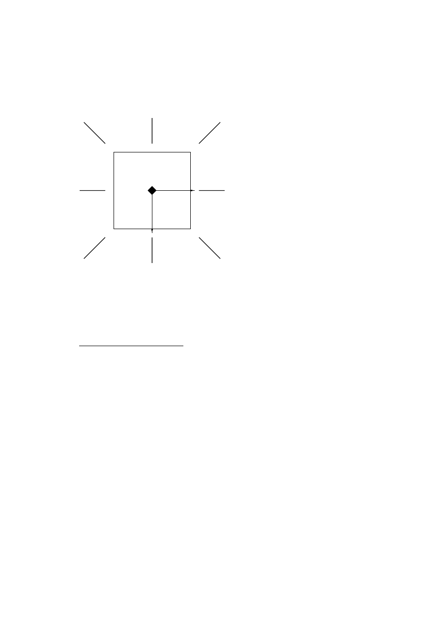
3.4
Crystallographic groups
39
Problem 1A. Symmetry of the square.
For the solution, see p. 73.
b
a
2
4
1
3
-1,-1
1,-1
-
1,1
-1,1
y
+
m
+
m
m
m
-
m
x
m
y
m
x
m
Fig. 3.4.1 The vertices 1, 2,
3, 4 of the square are de-
scribed by their coordinates
1, 1; –1, 1; –1, –1; 1, –1, re-
spectively. The coordinates
are referred to the axes a and
b and to the centre of the
square as origin.
Questions
For further questions, see Problem 1B, p. 63.
(i) List the symmetry operations of the square.
(ii) What is the geometric meaning of each of these symmetry
operations ?
(iii) What are the orders of these symmetry operations ?
(iv) How many symmetry operations of the square do exist ?

40
3
CRYSTALLOGRAPHIC SYMMETRY
Some remarks on space groups follow.
Space groups are the symmetries of crystal patterns, they have been defined already
by definition (D 3.2.1). Their order is always infinite because of the infinitely many
translations. Not only the order but also the number of space groups is infinite be-
cause each existing or conceivable crystal (crystal pattern) has ‘its’ space group.
However, an infinite set, as that of all space groups, is difficult to overlook. There-
fore, it is advantageous to have a classification of the space groups into a finite
number of classes.
The classification of site symmetries into types of site symmetries (crystal classes)
has already been discussed. Like site–symmetry groups, also space groups may
be classified into types, the space–group types. This classification into 230 space–
group types is so commonly used that these space–group types are just called the
230 space groups in many text books and in the spoken language. In most cases
there is no harm caused by this usage. However, for certain kinds of problems in
crystal chemistry, or when dealing with phase transitions, the distinction between
the individual ‘space group’ and the set ‘type of space groups’ is indispensable.
The distinction is important enough to be illustrated by an example from daily life:
There are millions of cars running on earth but there are only a few hundred types
of cars. One loosely says: ‘I have the same car as my neighbour’ when one means
‘My car is of the same type as that of my neighbour’. The difference becomes
obvious if the neighbour’s car is involved in a traffic accident.
Really, there are two classifications of space groups into types. The one just men-
tioned may be called the ‘classification into the 230 crystallographic space–group
types’. The different types are distinguished by the occurence of different types
of rotations, screw rotations, etc. (One cannot argue with the ‘numbers of 2–fold
rotations’ etc. because in space groups all these numbers are infinite). However,
there are 11 pairs of these types, called enantiomorphic pairs, where in each pair
the space groups of the one type can be transferred to those of the other type by
improper but not by proper mappings. (Proper and improper mappings are de-
fined in analogy to the proper and improper isometries, see Section 3.1. A pair of
enantiomorphic space–group types is analogous to a pair of gloves: right and left).
Counting each of these pairs as one type results in altogether 219 affine space–
group types.
More than 2/3 of the 911 pp. of Vol. IT A, 5th edition (2002) are devoted to the
description of the 17 ‘plane groups’ and the 230 ‘space groups’ (really: plane–
group and space–group types). There are four ways for this description; two of
them are described in the next section, the others in Sections 4.6 and 5.2.
The term point–symmetry group, point group, or point symmetry
P is used
in two different meanings. In order to have a clear distinction between the two
items which are commonly called ‘point symmetry’, the one item has been called
‘site–symmetry group’
S or ‘site symmetry’, see above. This is done also in IT
A, Section 8, ‘Introduction to space–group theory’. The other item is the external

3.4
Crystallographic groups
41
symmetry
P of the ideal macroscopic crystal. It is simultaneously the symmetry
of its physical properties. The symmetry
P is very much related to the symme-
try
S in so far as to each group S there exists a group P with the same order,
the same number and kind of rotations, rotoreflections and reflections, although
not necessarily in the same space group. Analogously, to each group
P there may
exist groups
S which have the same ‘structure’ as P has. Taken as groups with-
out paying attention to the kind of operations,
S and P cannot be distinguished.
Therefore, the statements 1. to 6., made above for groups
S, are valid for groups
P as well, with the exception of statement 2. The latter is obvious: A macroscopic
crystal is not periodic but ‘a massive block’ of finite extension, and there is only
one finite symmetry group
P for the external shape of the crystal as compared to
the infinite number of site–symmetry groups
S.
What is the essential difference between
S and P ? Why can they not be identi-
fied ?
The description of the symmetry
P is different from that of S. The relation be-
tween
S and the space group R is simple: S is a subgroup of R. The relation
between
P and R is more complicated and rather different. This will become clear
from the following example.
Example. There are not many compounds known whose symmetry consists of the
identity, translations and 2–fold rotations. The symbol of their space groups
R
1
is P
2. Several omphacites (rock-forming pyroxene minerals), high-temperature
Nb
2
O
5
, Cu
2
In
2
O
5
, and a few more compounds are reported to belong to space–
group type P
2.
The compound Li
2
SO
4
· H
2
O is the best pyroelectric non-ferroelectric substance
which is known today. Its space group
R
2
is P
2
1
with the identity, translations
and 2–fold screw rotations
2
1
. There are many compounds, e. g. sugars, with the
same kinds of symmetry operations.
Consider the points of point space. With regard to space group
R
1
, there are points
with site symmetry 2, namely all points situated on one of the 2–fold rotation axes.
However, with regard to space group
R
2
there is no point with site symmetry 2,
because screw rotations have no fixed points. Nevertheless, the symmetry of the
macroscopic crystal is that of (identity and) a 2–fold rotation in both cases. One
can say, that
R
1
and
R
2
have point groups of the same type, but exhibit strong
differences in their site–symmetry groups.
In order to understand this difference it is useful to consider the determination of
P. A natural crystal is mostly distorted: the growth velocities of its faces have been
influenced by currents of the medium from which the crystal has grown (liquid,
gas), or by obstacles which have prevented the development of the ideal shape.
Therefore, the faces present at a macroscopic crystal are replaced by their face
normals for the determination of the macroscopic symmetry. These face normals
are vectors which are independent of the state of development of the faces. Then
P
is determined from the symmetry operations which map the bundle of face–normal

42
3
CRYSTALLOGRAPHIC SYMMETRY
vectors onto itself. Thus, the group
P is a group of symmetry in vector space.
It is the conceptual difference between vector space and point space, experienced
already in Section 1.4 when considering origin shifts, which leads to the difference
between the groups
P and S. The symmetry operations of S are mappings of
point space, whereas the symmetry operations of
P are mappings of vector space.
In Section 4.4 the description of these operations by matrices will be dealt with.
It will turn out that the difference between
S and P is reflected in the kinds of
matrices which describe the operations of
S and P.
The above example of the space groups P
2 and P 2
1
has shown that there are space
groups for which the groups
P and S may have the same order, namely in P 2. This
is a special property which deserves a separate name.
Definition (D 3.4.3) A space group is called symmorphic if there are site–symmetry
groups
S which have the same order as the point group P of the space group.
In the non–symmorphic space group P
2
1
, there is no group
S with the order 2 of
P.
3.5
Display of crystallographic symmetry in IT A
A crystallographic symmetry operation may be visualized geometrically by its
‘geometric element’, mostly called symmetry element. The symmetry element is
a point, line, or plane related to the symmetry: depending on the symmetry op-
eration, it is the centre of inversion or (for rotoinversions) the inversion point;
the rotation, screw rotation, or rotoinversion axis; the mirror or glide plane. Only
the identity operation
I
and the translations
T
do not define a symmetry element.
Whereas the symmetry element of a symmetry operation is uniquely defined, more
than one symmetry operation may belong to a symmetry element. For example, to a
4–fold rotation axis belong the symmetry operations
4
1
= 4, 4
2
= 2 and 4
3
= 4
−1
around this axis.
[There is some confusion concerning the terms symmetry element and symmetry
operation. It is caused by the fact that symmetry operations are the group elements
of the symmetry groups (space groups, site–symmetry groups or point groups).
Symmetry operations can be combined resulting in other symmetry operations and
forming a symmetry group. Symmetry elements cannot be combined such that the
combination results in a uniquely determined other symmetry element. As a con-
sequence, symmetry elements do not form groups, and group theory cannot be
applied to them. Nevertheless, the description of symmetry by symmetry elements
is very useful, as will be seen now.]
In IT A, crystallographic symmetry is described in four ways:
1. The analytical description of symmetry operations by matrix-column pairs
will be considered in Chapter 4. The listing of these matrix–column pairs
as the ‘General position’ of IT A in a kind of short–hand notation will be
discussed in Section 4.6.

3.5
Display of crystallographic symmetry in IT A
43
2. The geometric meaning of the matrix–column pair can be determined, see
Section 5.2. In order to save the user this determination, in IT A the geomet-
ric meaning is listed for each matrix–column pair, see Section 4.6.
3. A visual geometric description of a space group (more exactly: a space–
group type) is possible by displaying the framework of symmetry elements
in a diagram, see this section.
4. In another diagram the space–group symmetry is represented by a set of
points which are symmetrically equivalent under the operations of the space
group, see this section.
In IT A, for each space group there are at least two diagrams displaying the sym-
metry (there are more diagrams for space groups of low symmetry). In this section
only one example for each kind of diagrams can be discussed in order to explain
the principles of this way of symmetry description. A full explanation of the details
is found in IT A, Section 2.6 ‘Space–group diagrams’, dto. in the Brief Teaching
Edition of IT A.
The Figs. 3.5.1 and 3.5.2 are taken from IT A, space-group table No. 86, P
4
2
/n
(HM symbol for this space–group type), C
4
4h
(S
CHOENFLIES
symbol for this
space–group type). In both diagrams, displayed is an orthogonal projection of a
unit cell of the crystal onto the paper plane. The direction of projection is the c
axis, the paper plane is the projection of the a–b plane (if c is perpendicular to a
and b, then the paper plane is the a–b plane). The thin lines outlining the projection
are the traces of the side planes of the unit cell. Because opposite lines represent
translationally equivalent side planes of the unit cell, the line pairs can be consid-
ered as representing the basic translations a and b. The origin (projection of all
points with coordinates 0 0 z) is placed in the upper left corner; the other vertices
represent the edges 1 0 z (lower left), 0 1 z (upper right) and 1 1 z (lower right).
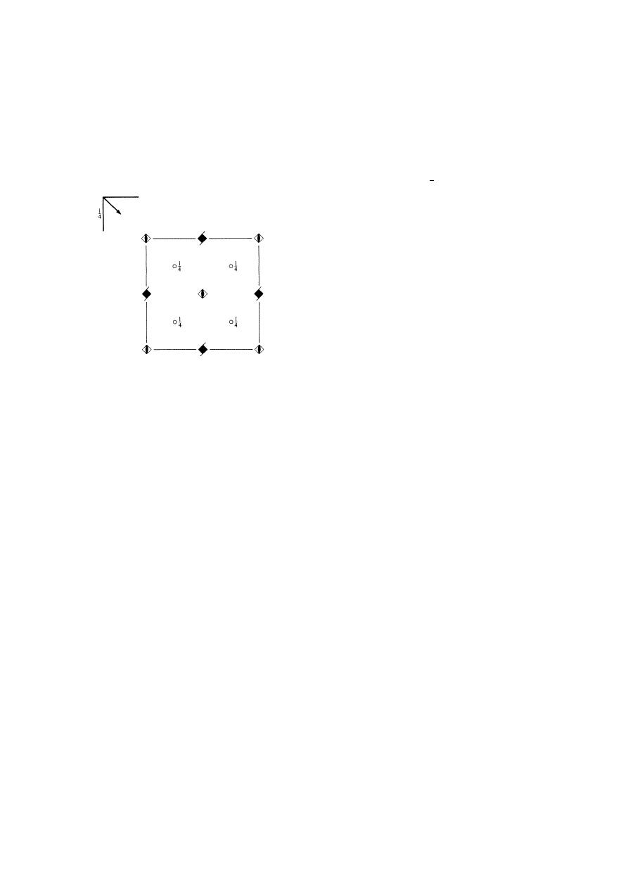
44
3
CRYSTALLOGRAPHIC SYMMETRY
The following diagram is always placed on the left side of the page in IT A.
Fig. 3.5.1 Symmetry elements. A
small circle represents a centre of
inversion ¯
1, the attached number
1
4
is its z coordinate (height above pa-
per in units of the lattice parameter
c). There are black squares with two
small tails: 4–fold screw-rotation
axes N
= 4, n = 2, see Sec-
tion 3.3, HM symbol
4
2
. A partly
filled empty square represents a 4–
fold rotoinversion axis, HM symbol
¯4. The ¯4 axes are parallel to c, they
are projected onto points. The right
angle drawn outside the top left of
the unit cell indicates a horizontal
glide plane with the direction of its
arrow as the glide vector. Missing
z coordinates mean either ‘z = 0’,
e. g. for the centres of ¯
4, or ‘z mean-
ingless’, as for the screw axes.
In the unit cell or on its borders are (only one representative of each set of transla-
tionally equivalent elements is listed):
(i) centres of inversion in 1/4, 1/4, 1/4; 1/4, 1/4, 3/4; 3/4, 1/4, 1/4;
3/4, 1/4, 3/4; 1/4, 3/4, 1/4; 1/4, 3/4, 3/4; 3/4, 3/4, 1/4; 3/4, 3/4, 3/4;
(ii)
4
2
axes in 1/2, 0, z; 0, 1/2, z;
(iii) ¯
4 axes in 0, 0, z; 1/2, 1/2, z with inversion points in 0, 0, 0; 0, 0, 1/2; 1/2, 1/2, 0;
1/2, 1/2, 1/2;
(iv) glide planes x, y,
1/4; x, y, 3/4 with glide vector 1/2, 1/2, 0.
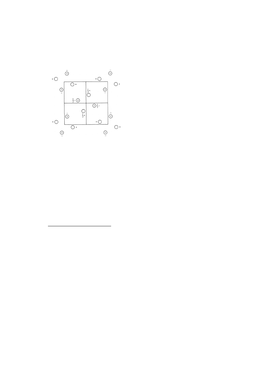
3.5
Display of crystallographic symmetry in IT A
45
The following diagram is always placed on the right side of the page in IT A.
Fig. 3.5.2 Starting with the point
in the upper left corner of the unit
cell, marked by an open circle and
with the sign ‘+’, all points in and
near the unit cell are drawn which
are images of the starting point un-
der some symmetry operation of the
space group. The starting point is
a point with site symmetry 1, i. e.
identity only. (Note that the high
symmetry of a circle does not re-
flect the site symmetry 1 of its cen-
tre properly. The circle is chosen for
historical reasons.) Then
all image points have site symmetry 1 too. The x and y coordinates of all points
can be taken from the projection; the z coordinate of the starting point is indicated
by ‘+’ (= +z), the other points have either ‘+’, or ‘
−’ (= −z), ‘1/2+’ (= 1/2 + z); or
‘
1/2−’ (= 1/2 −z); in other diagrams 1/4+, 1/4−, 3/4+, 3/4−, etc.
A ’–sign (comma) in the circle means that this point is an image of the starting
point by a symmetry operation of the second kind, see Section 3.1. If the empty
circles are assumed to represent right gloves, then the circles with a comma repre-
sent left gloves and vice versa.
The correspondence between the two diagrams is obvious: With some practice
each of the diagrams can be produced from the other. Therefore, they are com-
pletely equivalent descriptions of the same space–group symmetry. Nevertheless,
both diagrams are displayed in IT A in order to provide different aspects of the
same symmetry. Because of the periodicity of the arrangement, the presentation of
the contents of one unit cell is sufficient.
Answer
to the question in Section 3.2.
¯3
3
= ¯1, (¯3
6
= 1); ¯4
2
= 2; ¯6
2
= 3; and ¯6
3
= m, where the normal of the
mirror plane is parallel to the rotoinversion axis of ¯
6 (the mirror plane itself is
perpendicular to the rotoinversion axis).
The following statements hold always:
1. The even powers of rotoinversions are rotations.
2. The order of an N –fold rotoinversion is 2N for odd N .

46
4
THE DESCRIPTION OF MAPPINGS BY ... PAIRS
4
The description of mappings by matrix–column
pairs
4.1
Matrix–column pairs
As was mentioned already in Section 2.2, an affine mapping
A
is described by a
matrix A and a column a, see equations (2.2.1) and (2.2.5) on p. 19. Crystallo-
graphic symmetry operations are special affine mappings. They will be designated
by the letter
W
and described by the matrix W and the column w. Their description
is analogous to equation (2.2.1):
˜
x
= W
11
x + W
12
y + W
13
z + w
1
˜
y
= W
21
x + W
22
y + W
23
z + w
2
.
˜
z
= W
31
x + W
32
y + W
33
z + w
3
(4.1.1)
There are different ways of simplifying this array. One of them leads to the descrip-
tion with
Σ sign and indices in analogy to that for mappings, see equations (2.4.1)
and (2.4.2). It will not be followed here. Another one is the symbolic description
introduced in Section 2.3. It will be treated now in more detail.
Step 1
One writes the system of equations in the form
˜
x
˜
y
˜
z
=
W
11
W
12
W
13
W
21
W
22
W
23
W
31
W
32
W
33
x
y
z
+
w
1
w
2
w
3
.
(4.1.2)
The form 4.1.2 has the advantage that the coordinates and the coefficients which
describe the mapping are no longer intimately mixed but are more separated in
the equation. For actual calculations with concrete mappings this form is most
appropriate, applying the definitions (D 2.4.3) and (D 2.4.2). For the derivation of
general formulae, a further abstraction is advantageous.
Step 2
Denoting the coordinate columns by
˜x and x, the (3 × 3) matrix by
W and the column by w, one obtains in analogy to equation (2.2.5)
˜x = W x + w.
(4.1.3)
Step 3
Still the coordinate part and the mapping part are not completely
separated. Therefore, one writes
˜x = (W, w) x
or
˜x = (W | w) x.
(4.1.4)
The latter form is called the S
EITZ
notation.
Note that the forms (4.1.1) to (4.1.4) of the equations are only different ways of
describing the same mapping
W
. The matrix–column pairs (W, w) or (W
| w) are
suitable in particular for general considerations; they present the pure description
of the mapping, and the coordinates are completely eliminated. Therefore, in Sec-
tion 4.2 the pairs are used for the formulation of the combination
VU
of two sym-
metry operations
V
and
U
and of the inverse
W
−1
of a symmetry operation
W
.

4.2
Combination and reversion of mappings
47
However, if one wants to provide a list of specific mappings, then there is no way
to avoid the explicit description by the formulae 4.1.1 or 4.1.2, see Section 4.6.
With the matrix–column pairs one can replace geometric considerations by analyt-
ical calculations. To do this one first determines those matrix–column pairs which
describe the symmetry operations to be studied. This will be done in Section 5.1.
Then one performs the necessary procedures with the matrix–column pairs, e. g.
combination or reversion, see Section 4.2. Finally, one has to extract the geometric
meaning from the resulting matrix–column pairs. This last step is shown in Section
5.2.
4.2
Combination and reversion of mappings
The combination of two symmetry operations follows the procedure of Section
2.2. In analogy to equations (2.2.5) to (2.2.8) one obtains
˜x = Ux + u;
(4.2.1)
˜˜x = V˜x + v;
(4.2.2)
˜˜x = V(Ux + u) + v;
(4.2.3)
˜˜x = VUx + Vu + v = Wx + w.
(4.2.4)
These equations may be formulated with matrix–column pairs:
˜˜x = (V, v) ˜x = (V, v)(U, u)x = (W, w)x.
(4.2.5)
Note that in the product (V, v)(U, u) the operation (U, u) is performed first and
(V, v) second. Because of writing point coordinates and vector coefficients as
columns, in the combination of their mappings the sequence is always from right
to left.
By comparing equations (4.2.4) and (4.2.5) one obtains
(W, w) = (V, v)(U, u) = (VU, V u + v).
(4.2.6)
This law of composition for matrix–column pairs is not easy to keep in mind be-
cause of its asymmetry. It would be easy if the resulting matrix part would be the
product of the original matrices and the resulting column the sum of the original
columns. However, the column u of the operation, which is applied to the point X
first, is multiplied with the matrix V of the second operation, before the addition
is carried out. In the next section a formalism will be introduced which smoothes
out this awkwardness.

48
4
THE DESCRIPTION OF MAPPINGS BY ... PAIRS
The multiplication of matrix–column pairs is associative, because
(W, w)((V, v)(U, u)) = (W, w)(VU, Vu + v) =
= (WVU, WVu + Wv + w),
(4.2.7)
and on the other hand,
((W, w)(V, v))(U, u) = (WV, Wv + w)(U, u) =
= (WVU, WVu + Wv + w).
(4.2.8)
By comparison of both expressions one finds
(W, w)((V, v)(U, u)) = ((W, w)(V, v))(U, u).
(4.2.9)
Associativity is a very important property. It can be used, e. g., to find the value of
a product of matrix–column pairs without any effort. Suppose, that in the above
triple product of matrix–column pairs,
(W, w) = (V, v)
−1
holds and the upper
sequence of multiplications is to be calculated. Then, due to the associativity the
second equation may be used instead. Because
(V, v)
−1
(V, v) = (I, o) is the
identity mapping, the result ‘(U, u)’ is obtained immediately.
A linear mapping is a mapping which leaves the origin fixed. Its column part is
thus the o column. According to equation (4.2.6) any matrix–column pair can be
decomposed into a linear mapping (W, o) containing W only and a translation (I, w)
with w only:
(W, w) = (I, w)(W, o).
(4.2.10)
The linear mapping has to be performed first, the translation after that.
Question: What is the result if the translation (I, w) is performed first and the linear
mapping (W, o) after that, i. e. if the factors are exchanged ?
Before the reversion of a symmetry operation is dealt with, a general remark is
appropriate. In general, the formulae of this section are not restricted to crystallo-
graphic symmetry operations but are valid also for affine mappings. However, there
is one exception. In the inversion of a matrix W the determinant
det (W) appears
in the denominator of the coefficients of W
−1
, see Subsection 2.6.1. Therefore,
the condition
det (W) 6= 0 has to be fulfilled. Such mappings are called regular or
non–singular. Otherwise, if
det (W) = 0, the mapping is a projection and cannot
be reverted. For crystallographic symmetry operations, i. e. isometries
W
, always
det (W) = ±1 holds. Therefore, an isometry is always reversible, a general affine
mapping may not be. Projections are excluded from this manuscript because they
do not occur in crystallographic groups.
Now to the calculation of the reverse of a matrix–column pair. It is often necessary
to know which matrix C and column c belong to that symmetry operation
C
which
makes the original action
W
undone, i. e. which maps every image point ˜
X onto
the original point X. The operation
C
is called the reverse operation of
W
. The

4.2
Combination and reversion of mappings
49
combination of
W
with
C
restores the original state and the combined action
C W
maps X
→ ˜
X
→ X. It is the identity operation
I
which maps any point X onto
itself. The operation
I
is described by the matrix–column pair (I, o), where I is the
unit matrix and o is the column consisting of zeroes only. This means
x
= (C, c)˜x = C˜x + c
or
x
= Ix + o = (I, o)x = C(Wx + w) + c = CWx + Cw + c.
(4.2.11)
Equation (4.2.11) is valid for any coordinate triplet x. Therefore, the coefficients
on the right and left side are the same. It follows
CW
= I and Cw + c = o or C = W
−1
and W
−1
w
+ c = o,
i. e. (C, c) = (W, w)
−1
= (W
−1
,
−W
−1
w
).
(4.2.12)
This equation is as unpleasant as is equation (4.2.6). The matrix part is fine but
the column part is not just
−w as one would like to see but −w has to be mul-
tiplied with W
−1
. The next section will present a proposal how to overcome this
inconvenience.
It is always good to test the result of a calculation or derivation. One verifies the
validity of the equations
(W, w)
−1
(W, w) = (W, w)(W, w)
−1
= (I, o) by applying
equations (4.2.6) and (4.2.12). In addition in the following Problem 2A the results
of this section may be practised.
Problem 2A. Symmetry described by matrix–column pairs.
For the solution, see p. 75.
In Vol. A of International Tables for Crystallography the crystallographic symme-
try operations
A
,
B
, . . . are referred to a conventional coordinate system and are
represented by matrix–column pairs (A, a), (B, b), . . . . Among others one finds in
the space-group tables of IT A indirectly, see Section 4.6:
(A, a) =
0 1 0
1 0 0
0 0 ¯1
,
1/2
1/2
1/2
and (B, b) =
0 1 0
0 0 1
1 0 0
,
0
0
0
.
Combining two symmetry operations or reversion of a symmetry operation corre-
sponds to multiplication or reversion of these matrix–column pairs, such that the
resulting matrix–column pair represents the resulting symmetry operation.
The following calculations make use of the formulae 4.2.6 and 4.2.12.
Can one exploit the fact that the matrices A, B, C and D are orthogonal matrices ?
Questions
(i) What is the matrix–column pair resulting from
(B, b) (A, a) = (C, c) ?
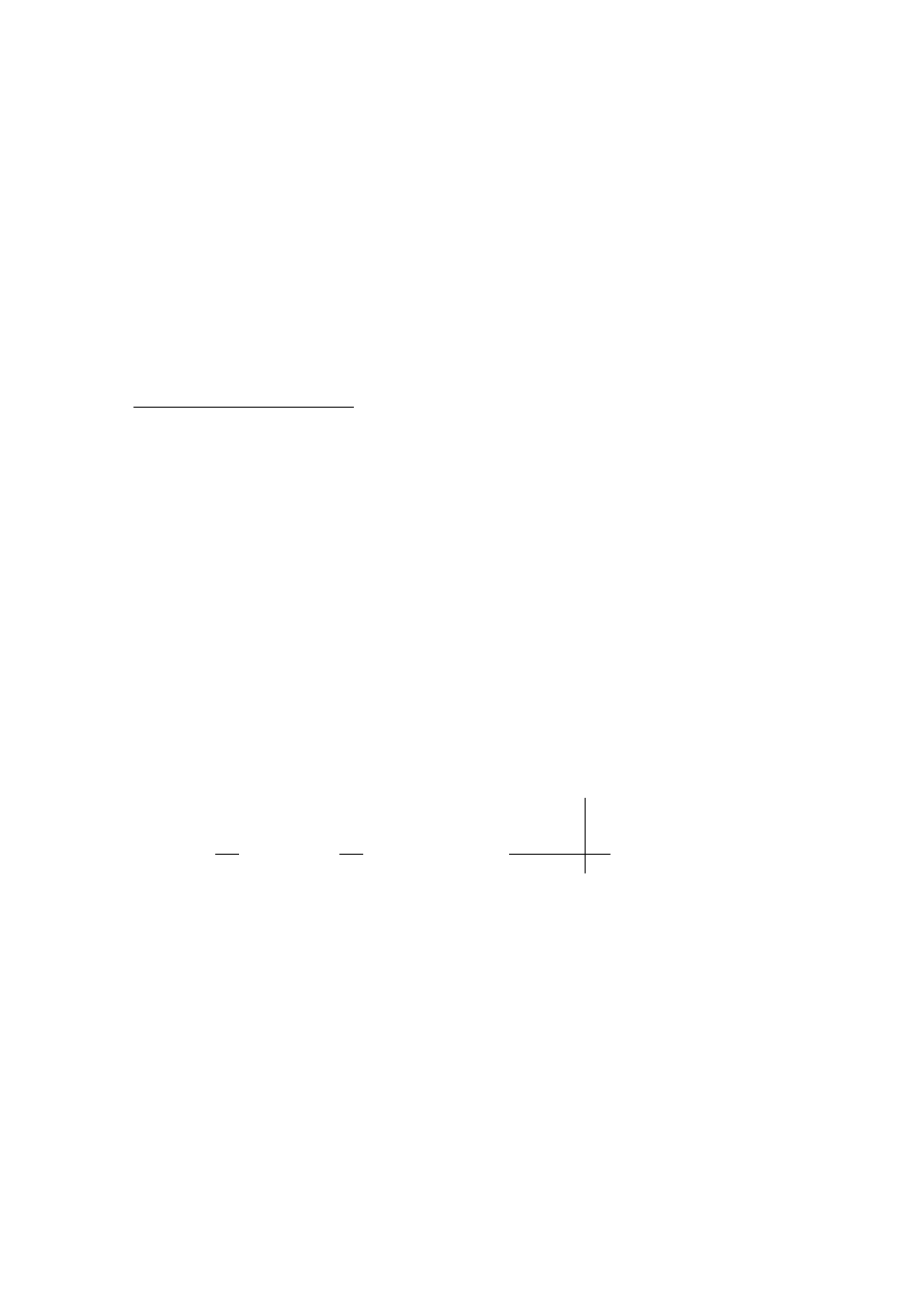
50
4
THE DESCRIPTION OF MAPPINGS BY ... PAIRS
(ii) What is the matrix–column pair resulting from
(A, a) (B, b) = (D, d) ?
(iii) What is (A, a)
−1
?
(iv) What is (B, b)
−1
?
(v) What is (C, c)
−1
?
(vi) What is (D, d)
−1
?
(vii) What is (B, b)
−1
(A, a)
−1
?
For another question of this Problem, see p. 66.
4.3
(
4 × 4) matrices
The formulae (4.2.6) and (4.2.12) are difficult to keep in mind. It would be fine to
have them in a more user–friendly shape. Such a shape exists and will be demon-
strated now. It is not only more convenient but also solves another problem, viz the
clear distinction between point coordinates and vector coefficients, as will be seen
in Section 4.4.
If a crystallographic symmetry operation is described by the matrix–column pair
(W, w), then one can form the
(3 × 4) matrix
W
11
W
12
W
13
w
1
W
21
W
22
W
23
w
2
W
31
W
32
W
33
w
3
.
Regrettably, such matrices cannot be multi-
plied with each other because of the different
number (4) of columns of the left matrix and
(3) of rows of the right matrix, see Section 2.4.
However, one can make the matrix square by
adding a fourth row ‘0 0 0 1’. Such
(4 × 4)
matrices can be multiplied with each other. For the applications also the coordinate
columns have to be extended. This is done by adding a fourth row with the number
1 to the
(3 × 1) column. We thus have:
x
→
x
=
x
y
z
1
; ˜x → ˜
x
=
˜
x
˜
y
˜
z
1
; (W, w) →
W
=
W
w
0
0
0
1
.
(4.3.1)
Definition (D 4.3.1) The
(4 × 4) matrix
W
obtained from W and w in the way just
described is called the augmented matrix
W
; the columns are called augmented
columns.
The horizontal and vertical lines in the matrix and the horizontal line in the columns
have no mathematical meaning; they are to remind the user of the geometric con-
tents and of the way in which the matrix has been built up.
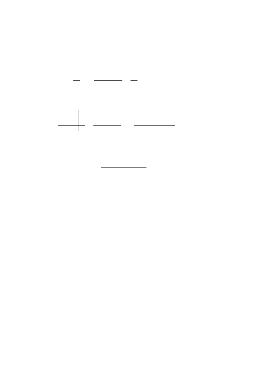
4.4
Transformation of vector coefficients
51
Equation (4.1.2) is replaced by an equation in outlined letters
˜
x
˜
y
˜
z
1
=
W
w
0
0
0
1
x
y
z
1
or ˜
x
=
W
x
.
(4.3.2)
The augmented matrices may be multiplied, and the product is indeed a
(4×4) ma-
trix whose matrix and column parts are the same as those obtained from equation
(4.2.6):
V
v
0
0
0 1
U
u
0
0
0 1
=
VU
Vu
+ v
0
0
0
1
.
(4.3.3)
For the reverse mapping
W
−1
,
W
−1
W
=
I
holds, where
I
is the (
4 × 4) unit
matrix. This is fulfilled for
W
−1
=
W
−1
−W
−1
w
0
0
0
1
,
(4.3.4)
which corresponds to equation (4.2.12).
In practice the augmented quantities are very convenient for general formulae and
for the actual combination of mappings by multiplying
(4 × 4) matrices. Equation
(4.3.4) is useful to provide the inverse of a
(4 × 4) matrix by calculating the right
side. It does not make sense to invert a
(4 × 4) matrix using equation (2.6.1) on p.
28 for direct matrix inversion.
In an analogous way one can describe mappings of the plane by
(3×3) augmented
matrices and
(3 × 1) augmented columns.
4.4
Transformation of vector coefficients
It has already been demonstrated, in Section 1.4, that point coordinates and vector
coefficients display a different behaviour when the coordinate origin is shifted. The
same happens when a translation is applied to a pair of points. The coordinates of
the points will be changed according to
˜x = (I, t) x = x + t; ˜y = (I, t) y = y + t.
However, the distance between the points will be invariant:
˜y
− ˜x = (y + t) − (x + t) = y − x.
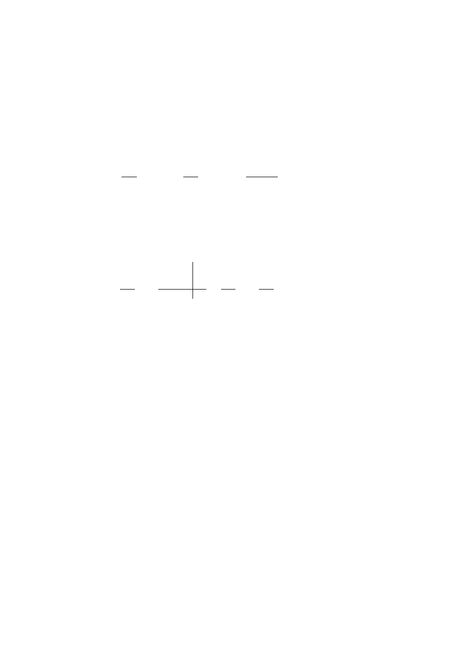
52
4
THE DESCRIPTION OF MAPPINGS BY ... PAIRS
Distances are absolute values of vectors, see Section 1.6. Usually point coordinates
and vector coefficients are described by the same kind of
(3 × 1) columns and are
difficult to distinguish. It is a great advantage of the augmented columns to provide
a clear distinction between these quantities.
If
x
x
and
x
y
are the augmented columns of coordinates of the points X and Y ,
x
x
=
x
1
x
2
x
3
1
and
x
y
=
y
1
y
2
y
3
1
, then
r
=
y
1
− x
1
y
2
− x
2
y
3
− x
3
0
is the augmented column
r
of the coefficients of the distance vector r between
X and Y . The last coefficient of
r
is zero, because of
1 − 1 = 0. It follows that
columns of vector coefficients are augmented in another way than columns of point
coordinates.
Let
T
be a translation, (I, t) its matrix–column pair,
T
its augmented matrix, r the
(3 × 1) column of coefficients of the distance vector r between X and Y , and
r
the
augmented column of r. Then,
˜
r
=
Tr
or
˜
r
1
˜
r
2
˜
r
3
0
=
t
1
I
t
2
t
3
0 0 0
1
r
1
r
2
r
3
0
=
r
1
r
2
r
3
0
.
(4.4.1)
When using augmented columns and matrices, the coefficients of t are multiplied
with the last coefficient 0 of the
r
column and thus become ineffective.
This behaviour is valid not only for translations but holds in general for affine
mappings, and thus for isometries and crystallographic symmetry operations:
y
− x → ˜y − ˜x = (W y + w) − (W x + w) = W y − W x = W(y − x) or
˜
r
=
W
r
=⇒ ˜r = W r + 0 w = W r.
(4.4.2)
Whereas point coordinates are transformed by
˜x = (W, w)x = W x + w,
vector coefficients r are affected only by the matrix part W:
˜r = (W, w)r = W r.
(4.4.3)
In other words: if (W,w) describes an affine mapping (isometry, crystallographic
symmetry operation) in point space, then W describes the corresponding mapping
in vector space. For vector coefficients, the column part w does not contribute to
the mapping. This is valid for any vector, e. g., also for the basis vectors of the
coordinate system.
Note that
˜y
− ˜x = W(y − x) is different from ( ]
y
− x) = W(y − x) + w. The
latter expression describes the image point ˜
Z of the point Z with the coordinates
z
= y − x.

4.5
The matrix-column pairs of crystallographic symmetry operations
53
4.5
The matrix-column pairs of crystallographic symmetry op-
erations
For general matrices, multiplication and inversion may be rather tedious manipu-
lations. These are unavoidable if the geometry of the object is complicated and if
there is no way to simplify it. In crystallography one is in a better situation. By def-
inition crystals are periodic, and their periodicity is not that of the continuum but
that of the lattice. Therefore, primitive bases for the lattices can always be found,
see definition (D 1.5.2). As a consequence, the matrix–column pairs for the crys-
tallographic symmetry operations are simple if an appropriate coordinate system
has been chosen. The conventional coordinate systems as used in the space– and
plane–group tables of IT A are chosen under this aspect.
The matrix parts shall be considered first.
Suppose, a primitive lattice basis has been chosen as the coordinate basis. We take
from the last section that the mapping of vectors by a crystallographic symme-
try operation
W
is described only by the matrix part W of the
(4 × 4) matrix
W
. The image of a lattice vector under a symmetry operation must be a lattice
vector, otherwise the lattice would not be mapped onto itself as a whole. Being
referred to a primitive basis, all lattice vectors have integer coefficients. Therefore,
the matrix parts W of the crystallographic symmetry operations must have integer
coefficients, they are integer matrices.
On the other hand, a crystallographic symmetry operation
W
is an isometry. There-
fore, referred to an orthonormal basis, the matrix is an orthogonal matrix, see Sub-
section 2.6.1, p. 28. When leaving all distances invariant, also the volume is invari-
ant. Analytically, this means
det(W) = ±1.
If a matrix is integer and orthogonal, then in each row and column there are exactly
one entry
±1 and two zeroes. The matrix has thus three coefficients ±1 and six ze-
roes. How many
(3 × 3) matrices of this kind do exist ? There are six arrangements
to distribute the non–zero coefficients among the positions of the matrix. In addi-
tion, there are three signs with
2
3
possibilities of distributing + and
−. Altogether
there are
6 × 8 = 48 different orthogonal integer matrices.
The matrix parts of crystallographic symmetry operations form groups which de-
scribe the point groups, see Sections 3.4 and 4.4. The highest order of a crystallo-
graphic point group is 48, and referred to the conventional basis this point group is
described by the group of the 48 orthogonal integer matrices. It is the point group
of copper, gold, rocksalt, fluorite, galena, garnet, spinel and many other crystalline
compounds. The symmetries of 24 other point groups are contained as subgroups
in this highest symmetry, so that 25 of the 32 types of point groups (crystal classes)
can be described by orthogonal integer matrices. The advantages of these matrices
are:
1. The product of two matrices is easily calculated because of the many zeroes;
it is again an orthogonal integer matrix.

54
4
THE DESCRIPTION OF MAPPINGS BY ... PAIRS
2. Due to the orthogonality, the inverse of a matrix is the transpose matrix and
does not need calculation.
3. The determinant of a matrix, see equation 2.5.2, is the product of three co-
efficients
±1, adjusted for the sign.
What about the necessary bases ? The matrix part of an isometry is orthogonal if
referred to an orthonormal basis; it may also be orthogonal if referred to another
basis. The restrictions to the basis depend on the point group. For example, the
matrices describing the identity mapping and the inversion are orthogonal in any
basis, viz the unit matrix and the negative unit matrix. The conventional bases in
crystallography are lattice bases (not orthonormal bases). They are mostly chosen
such that the matrices are integer orthogonal matrices. As already mentioned, this
is possible for 25 of the 32 crystal classes of point groups.
The matrix is even simpler, if it is a diagonal orthogonal matrix, i. e. a diagonal
matrix with coefficients
±1. There are 2
3
= 8 such matrices, among them the
unit matrix I and the inversion ¯
I. If the symmetry of the crystal is low enough, all
matrices are diagonal. There are eight crystal classes (of the 25) permitting such a
description. Crystals with this symmetry are also called optically biaxial crystals
because of their optical properties (birefringence).
The point groups of the remaining seven crystal classes cannot be described by
orthogonal integer matrices. Referred to a primitive basis, their matrices are in-
teger, of course. However, this representation is not orthogonal. One can choose
an orthonormal basis instead but then the matrices are no longer integer matrices.
These point groups are hexagonal and belong to the hexagonal crystal family.
Only in crystal physics the non–integer orthogonal representation is used for hexag-
onal point groups, in crystallography the representation by integer matrices is pre-
ferred. One introduces the so–called hexagonal basis, referred to which the ma-
trices consist of at least five zeroes and four coefficients
±1. In the conventional
settings of IT A, there occur up to 16 such matrices, the other up to eight matri-
ces are orthogonal integer matrices. Although not necessary, also trigonal point
groups are mostly referred to the hexagonal basis, because this description is for
many crystals more natural than the decription by integer orthogonal matrices.
The column parts will be discussed now.
Provided a conventional coordinate system is chosen, also the coefficients of the
columns are simple. They are determined
1. by the choice of the basis which, however, is more or less fixed already by
the matrix considerations.
2. by the origin choice. If the origin is chosen in a fixed point of a symmetry
operation
W
, then w is the o column. Clearly, one choice of the origin is
such that as many of the symmetry operations as possible have the origin as
fixed point.

4.6
The ‘General Position’ in IT A
55
Doing this it turns out, that the remaining non-zero coefficients of the columns w
are fractions with denominators at most 6.
4.6
The ‘General Position’ in IT A
In IT A the set of all symmetry operations is listed for all space groups. As we
have seen, space groups are infinite groups, and there is an infinite number of
space groups for each space–group type, see Section 3.4. How can such a listing
be done at all ? In this section the principles are dealt with which make the listings
possible, as well as the points of view which determine the actual listings.
1. Consider the infinite number of space groups belonging to a certain space–
group type. If one refers each space group to its conventional coordinate
system, one obtains a set of matrix–column pairs for each space group but
all these sets are identical. (This is one way to classify the space groups into
space–group types.) Therefore, a listing is necessary only for each space–
group type, but not for each space group. This means 230 listings for the
space groups and 17 listings for the plane groups, and these listings are in-
deed contained in IT A. In reality the number of space–group listings is
higher by about 20 % because there is sometimes more than one conven-
tional coordinate system: different settings, different bases, or different ori-
gins, see IT A.
2. No doubt, there is an infinite number of symmetry operations for each space
group. How can they be listed in a book of finite volume ? Let
W
be a
symmetry operation and (W, w) its matrix–column pair. Because the con-
ventional bases are always lattice bases, (W, w) can be decomposed into a
translation
(I, t
n
) with integer coefficients and the matrix (W, w
◦
):
(W, w) = (W, w
◦
+ t
n
) = (I, t
n
)(W, w
◦
).
(4.6.1)
For the coefficients w
◦
, 0 ≤ w
i◦
< 1 holds. By this decomposition one
splits the infinite set of pairs (W, w) into a finite set of representatives
(W, w
◦
)
and an infinite set of translations
(I, t
n
). Clearly, only the representatives
need to be listed. Such a list is contained in IT A for each space–group type;
the number of necessary entries is reduced from infinite to at most 48.
For primitive bases, the list is complete and unique. There are ambiguities
for centred settings, see the remarks to definition (D 1.5.2). For example, for
a space group with an I–centred lattice, to each point x, y, z there belongs a
translationally equivalent point x
+1/2, y+1/2, z+1/2. Nevertheless, only
one entry
(W, w
◦
) is listed. Again, instead of listing a translationally equiv-
alent pair for each entry, the centring translation is extracted from the list
and written once for all on top of the listing. For example, the rational trans-
lations for the I–centred lattice are indicated by ‘(0, 0, 0)+
(
1
2
,
1
2
,
1
2
)+’.
For each of the matrix–column pairs
(W, w
◦
), listed in the sequel, not only

56
4
THE DESCRIPTION OF MAPPINGS BY ... PAIRS
the products
(I, t
n
)(W, w
◦
) have to be taken into account, but also the prod-
ucts
(I, t
n
+
1
2
)(W, w
◦
). (The term
1
2
is a symbol for the column with all
coefficients
1
2
.) The following example 3 (General position for space–group
type I
2
1
3, No. 199) provides such a listing.
3. The representatives
(W, w
◦
) could be listed as matrix–column pairs but that
would be wasting space. Although one could not save much space with fur-
ther conventions when listing general matrices, the simple (48 orthogonal +
16 other = 64) standard matrices of crystallography with their many zeroes
have a great potential for rationalization. Is there any point to list thousands
of zeroes ? Therefore, in crystallography an efficient procedure is applied
to condense the description of symmetry by matrix–column pairs consid-
erably. This method works like the shorthand notation for the normal lan-
guage, when the usual letters are replaced by shorthand symbols.
The equations (4.1.1) on p. 46 are shortened in the following way:
(a) The left side and the ‘=’ sign are omitted
(b) On the right side, all terms with coefficients 0 are omitted
(c) Coefficients ‘+1’ are omitted, coefficients ‘–1’ are replaced by ‘–’ and
are frequently written on top of the variable: x instead of
−x, etc.
(d) The three different rows are written in one line but separated by com-
mas.
3 examples shall display the procedure.
Example 1.
˜x = (W, w)x =
0 1 0
¯1 0 0
0 0 1
x
y
z
+
1/2
1/2
1/4
would be
˜
x = 0 x + 1 y + 0 z + 1/2, ˜
y = −1 x + 0 y + 0 z + 1/2, ˜
z = 0 x + 0 y + 1 z + 1/4.
The shorthand notation of IT A reads
y + 1/2, x + 1/2, z + 1/4.
It is found in IT A under space group P
4
3
2
1
2, No. 96 on p. 376. There it is entry
(4) of the first block (the so–called General position) under the heading Positions.
Example 2.
˜x = (W, w)x =
0 1 0
¯1 1 0
0 0 1
x
y
z
+
0
0
1/2
is written in the shorthand notation of IT A
y, x
+ y, z + 1/2;
space group P
6
3
mc, No. 186 on p. 584 of IT A.
It is entry (5) of the General position.
Example 3.
The following table is the actual listing of the General position
for space–group type I
2
1
3, No. 199 in IT A on p. 612. The 12 entries, numbered

4.6
The ‘General Position’ in IT A
57
(1) to (12), are to be taken as they are (indicated by (0, 0, 0)+) and in addition with
1/2 added to each element w
i◦
(indicated by
(
1
2
,
1
2
,
1
2
)+). Altogether these are 24
entries, which is announced by the first number in the row, the ‘Multiplicity’. The
reader is recommended to convert some of the entries into matrix–column pairs or
(4 × 4) matrices.
Positions
Multiplicity,
Wyckoff letter,
Coordinates
Site symmetry
(0, 0, 0) +
(
1
2
,
1
2
,
1
2
)+
24 c 1 (1) x, y, z
(2) x +
1
2
, y, z +
1
2
(3) x, y +
1
2
, z +
1
2
(4) x +
1
2
, y +
1
2
, z
(5) z, x, y
(6) z +
1
2
, x +
1
2
, y
(7) z +
1
2
, x, y +
1
2
(8) z, x +
1
2
, y +
1
2
(9) y, z, x (10) y, z +
1
2
, x +
1
2
(11) y +
1
2
, z +
1
2
, x
(12) y +
1
2
, z, x +
1
2
The listing of the ‘General position’ kills two birds with one stone:
(i) each of the numbered entries lists the coordinates of an image point ˜
X of
the original point X under a symmetry operation of the space group.
(ii) Each of the numbered entries of the General position lists a symmetry op-
eration of the space group by the shorthand notation of the matrix–column
pair. This fact is not as obvious as the meaning described under (i) but it is
much more important. Knowing this way one can extract and make available
for calculations the full analytical symmetry information of the space group
from the tables of IT A.
Exactly one image point belongs to each of the infinitely many symmetry oper-
ations and vice versa. Some of these points are displayed in Figure 3.5.2 on p.
45.
Definition (D 4.6.1) The set of all points which are symmetrically equivalent to a
starting point X (and thus to each other) under the symmetry operations of a space
group
R is called a point orbit R X of the space group.
Remarks.
1. The starting point is a point of the orbit because it is mapped onto itself
by the identity operation (I, o) which is a symmetry operation of any space
group.
2. The one–to–one correspondence between symmetry operations and points
is valid only for the General position, i. e. the first block from top in the
space–group tables. In this block the coordinate triplets (shorthand symbols
for symmetry operations) refer to points which have site symmetry
I, i. e.
only the identity operation is a symmetry operation. In all the other blocks,
the points have site symmetries
S > I with more than one site-symmetry

58
4
THE DESCRIPTION OF MAPPINGS BY ... PAIRS
operation. If
S > I, also |S| > 1 holds, where |S| is the order of S. One can
show, that the point X is mapped onto its image ˜
X by exactly as many sym-
metry operations of the space group
R as is the order of the site–symmetry
group
S of X. Therefore, for such points the symmetry operation cannot be
derived from the data listed in IT A because it is not uniquely determined.
Definition (D 4.6.2) The blocks with points of site symmetries
S > I are called
special positions.
Different from the General position, a coordinate triplet of a special position pro-
vides the coordinates
˜
x, ˜
y, ˜
z of the image point of the starting point x, y, z only
but no information on a matrix–column pair.

59
5
Special aspects of the matrix formalism
The contents of this chapter serve two purposes:
1. To forge a link between geometry and calculations;
2. To provide the tools for coordinate changes.
The first point is described in the first two sections. The questions to be discussed
are:
(i) How can the matrix–column pair be obtained when the geometric meaning
of the symmetry operation is known ?
(ii) Given a matrix–column pair, what is its geometric meaning ?
The second point is a practical one. The complexity and amount of calculations
depend strongly on the coordinate system of reference for the geometric actions.
Therefore, it is advantageous to be flexible and free to choose for each calcula-
tion the optimal coordinate system. This means to change the coordinate system if
necessary and to know what happens with the coordinates and the matrix–column
pairs by such a change. In the last section of this chapter, partitioned into three
subsections, coordinate changes will be treated in three steps: Origin shift, change
of basis and change of both, i. e. general coordinate changes.
5.1
Determination of the matrix-column pair
In this section it is assumed that not only the kind of symmetry operation is known
but also its details, e. g. it is not enough to know that there is a 2–fold rotation, but
one should also know the orientation and position of the rotation axis. At first one
tries to find for some points X their images ˜
X under the symmetry operation. This
knowledge is then exploited to determine the matrix–column pair which decribes
the symmetry operation.
Examples will illustrate the procedures. In all of them the point coordinates are
referred to a Cartesian coordinate system, see Section 1.2. The reader is recom-
mended to make small sketches in order to see visually what happens.
In the system (4.1.1) of equations there are 12 coefficients to be determined, 9
W
ik
and 3 w
j
. If the image point ˜
X of one point X is known from geometric
considerations, one can write down the three linear equations of (4.1.1) for this
pair of points. Therefore, writing down the equations (4.1.1) for four pairs (point
→ image point) is sufficient for the determination of all coefficients, provided the
points are independent, i. e. are not lying in a plane. One obtains a system of 12
inhomogeneous linear equations with 12 undetermined parameters W
ik
and w
j
.
This may be difficult to solve without a computer. However, if one restricts to
crystallographic symmetry operations, the solution is easy more often than not
because of the special form of the matrix–column pairs.

60
5
SPECIAL ASPECTS OF THE MATRIX FORMALISM
Procedure 1
In many cases it may be possible to apply the following strategy, which avoids all
calculations. It requires knowledge of the image points of the origin O and of the
3 ‘coordinate points’ A: 1, 0, 0; B: 0, 1, 0; and C: 0, 0, 1.
(1)
The origin
Let ˜
O with coordinates
˜o be the image of the origin O with
coordinates o, i. e. x
◦
= y
◦
= z
◦
= 0. Examination of the equations (4.1.1)
shows that
˜o = w, i. e. the column w can be determined separately from the
coefficients of the matrix W without any effort.
(2)
The coordinate points
We consider the point A. Inserting 1, 0, 0 in the
equations (4.1.1) one obtains
˜
x
i
= W
i1
+ w
i
or W
i1
= ˜
x
i
− w
i
, i
= 1, 2, 3.
The first column of W is separated from the others, and for the solution
only the known coefficients w
i
have to be subtracted from the coordinates
˜
x
i
of the image point ˜
A of A. Analogously one calculates the coefficients
W
i2
from the image of point B: 0, 1, 0 and W
i3
from the image of point C:
0, 0, 1.
Evidently, the sought after coefficients can be determined without any difficult
calculation.
Example 1
What is the pair (W, w) for a glide reflection with the plane through the origin, the
normal of the glide plane parallel to c, and with the glide vector g = 1/2, 1/2, 0 ?
(a) Image of the origin O: The origin is left invariant by the reflection part of the
mapping; it is shifted by the glide part to 1/2, 1/2, 0 which are the coordinates
of ˜
O. Therefore, w = 1/2, 1/2, 0.
(b) Images of the coordinate points. Both the points A and B are not affected
by the reflection part but A is then shifted to 3/2, 1/2, 0 and B to 1/2, 3/2, 0.
This results in the equations
3/2 = W
11
+ 1/2,
1/2 = W
21
+ 1/2,
0 = W
31
+ 0
for A
and
1/2 = W
12
+ 1/2,
3/2 = W
22
+ 1/2,
0 = W
32
+ 0
for B.
One obtains W
11
= 1, W
21
= W
31
= W
12
= 0, W
22
= 1 and W
32
= 0.
Point C: 0, 0, 1 is reflected to 0, 0,
−1 and then shifted to 1/2, 1/2, −1.
This means
1/2 = W
13
+ 1/2, 1/2 = W
23
+ 1/2, −1 = W
33
+ 0
or
W
13
= W
23
= 0, W
33
= −1.
(c) The matrix–column pair is thus
W =
1 0 0
0 1 0
0 0 ¯1
and w =
1/2
1/2
0
.

5.1
Determination of the matrix-column pair
61
Tests for the correctness of the result are always advisable: Each point x, y,
0 is
mapped onto the point x
+ 1/2, y + 1/2, 0, i. e. the plane x, y, 0 is invariant as
a whole; each point x, x, z is mapped onto x
+ 1/2, x + 1/2, −z, i. e. the plane
x, x, z is also left invariant as a whole. Both results agree with the geometric view.
Example 2
[Draw a diagram !]
What is the pair (W, w) for an anti–clockwise 4–fold rotoinversion ¯
4 if the rotoin-
version axis is parallel to c, and 1/2, 1/2, 1/2 is the inversion point ?
(a) The anti–clockwise 4–fold rotation maps the origin onto the point 1, 0, 0;
the following inversion in 1/2, 1/2, 1/2 maps this intermediate point onto the
point 0, 1, 1, such that w
1
= 0, w
2
= 1, w
3
= 1.
(b) For the other points:
1, 0, 0 → 1, 1, 0 → 0, 0, 1;
0, 1, 0 → 0, 0, 0, → 1, 1, 1;
0, 0, 1 → 1, 0, 1 → 0, 1, 0.
The equations are
0 = W
11
+ 0; 0 = W
21
+ 1; 1 = W
31
+ 1;
1 = W
12
+ 0; 1 = W
22
+ 1; 1 = W
32
+ 1;
0 = W
13
+ 0; 1 = W
23
+ 1; 0 = W
33
+ 1.
(c) The result is
W =
0 1 0
¯1 0 0
0 0 ¯1
; w =
0
1
1
.
The resulting matrix–column pair is checked by mapping the fixed point 1/2, 1/2, 1/2
and the point 1/2, 1/2, 0. Their images are 1/2, 1/2, 1/2 and 1/2, 1/2, 1 in agreement
with the geometric meaning of the operation.
Procedure 2
If the images of the origin and/or the coordinate points are not known, other pairs
‘point–image point’ must be used. It is difficult to give general rules but often fixed
points are appropriate in such a case. In addition, one may exploit the different
transformation behaviour of point coordinates and vector coefficients, see Section
4.4. Vector coefficients ‘see’ only the matrix W and not the column w, and that
may facilitate the solution. Nevertheless, the calculations may now become more
involved. The next example is not crystallographic in the usual sense, but related
to twinning in ‘spinel’ mineral.
Example 3
What is the pair (W, w) for a 2–fold rotation about the space diagonal [1 1 1] with
the point 1/2, 0, 0 lying on the rotation axis ?
It is not particularly easy to find the coordinates of the image ˜
O of the origin O.
Therefore, another procedure seems to be more promising. One can use the trans-
formation behaviour of the vector coefficients of the direction [1 1 1] and other

62
5
SPECIAL ASPECTS OF THE MATRIX FORMALISM
distinguished directions. The direction [1 1 1 ] is invariant under the 2–fold rota-
tion, and the latter is described by the matrix part only, see Section 4.4. Therefore,
the following equations hold
1 = W
11
+W
12
+W
13
, 1 = W
21
+W
22
+W
23
, 1 = W
31
+W
32
+W
33
. (5.1.1)
On the other hand, the directions [1 ¯
1 0], [0 1 ¯1], and [¯1 0 1] are perpendicular to
[1 1 1] and thus are mapped onto their negative directions. This means
[1 ¯1 0] :
[0 1 ¯1] :
[¯1 0 1] :
−1 = W
11
− W
12
,
0 = W
12
− W
13
,
1 = −W
11
+ W
13
,
1 = W
21
− W
22
,
−1 = W
22
− W
23
,
0 = −W
21
+ W
23
,
0 = W
31
− W
32
,
1 = W
32
− W
33
,
−1 = −W
31
+ W
33
,
.
(5.1.2)
From the equations (5.1.2) one concludes
W
12
= W
13
,
W
21
= W
23
,
W
31
= W
32
W
11
= W
13
− 1, W
22
= W
21
− 1, W
33
= W
32
− 1.
Together with equations (5.1.1) one obtains
W
11
= W
22
= W
33
= −1/3; W
12
= W
13
= W
21
= W
23
= W
31
= W
32
=
2/3.
Thus, W =
−1/3
2/3
2/3
2/3 −1/3
2/3
2/3
2/3 −1/3
.
The point 1/2 0 0 is a fixed point, thus
1/2 = −1/3 · 1/2 + 2/3 · 0 + 2/3 · 0 + w
1
,
0 = 2/3 · 1/2 − 1/3 · 0 + 2/3 · 0 + w
2
and
0 = 2/3 · 1/2 + 2/3 · 0 − 1/3 · 0 + w
3
.
The coefficients of w are then: w
1
= 2/3, w
2
= −1/3, w
3
= −1/3.
There are different tests for the matrix: It is orthogonal, its order is 2 (because
it is orthogonal and symmetric), its determinant is
+1, it leaves the vector [1 1 1]
invariant, and maps the vectors
[1 ¯1 0], [0 1 ¯1] and [¯1 0 1] onto their negatives (as
was used for its construction). The matrix–column pair can be tested with the fixed
points, e. g. with
1/2, 0, 0; with 1/2, 0, 0 + 1, 1, 1 = 3/2, 1, 1; or other points
on the rotation axis.

5.2
The geometric meaning of (
W
,
w
)
63
Problem 1B. Symmetry of the square.
For the solution, see p. 74.
Problem 1A, p. 39, dealt with the symmetry of the square, see Fig. 3.4.1.
There are two more questions concerning this problem.
(v) Calculate the matrix–column pairs of the symmetry operations of the square.
(vi) Construct the multiplication table of the group of the square. [The multipli-
cation table of a group
G of order N is a table with N rows and N columns.
The elements of the group are written on top of the table and on the left side,
preferably in the same sequence and starting with the unit element. In the in-
tersection of the ith row and the kth column the product
W
i
W
k
is listed for
any pair of indices
1 ≤ i, k ≤ N . The complete table is the multiplication
table].
Are there remarkable properties of the multiplication table ?
5.2
The geometric meaning of (W, w)
How can one find the geometric meaning of a matrix–column pair ? Large parts of
the following recipe apply not only to crystallographic symmetry operations but
also to general isometries.
1. One must know the reference coordinate system of the matrix–column pair.
Without this knowledge a geometric evaluation is impossible.
Example.
The matrix (in IT A shorthand notation) x
−y, x, z describes
a 6–fold anti–clockwise rotation if referred to a hexagonal basis. If referred
to an orthonormal basis it does not describe an isometry at all but contains a
shearing component.
2. The matrix part is evaluated first.
In general the coefficients of the matrix depend on the choice of the ba-
sis; a change of basis changes the coefficients, see Section 5.3.2. However,
there are geometric quantities which are independent of the basis. Corre-
spondingly, there exist characteristic numbers of a matrix from which the
geometric features may be derived and vice versa.
– The preservation of the ‘handedness’ of an object, i. e. the question if
the symmetry operation is a rotation or rotoinversion is a geometric
property. The corresponding property of the matrix is its determinant:
det(W) = +1: rotation;
det(W) = −1: rotoinversion.
– The angle of rotation ϕ. It does not depend on the coordinate basis.
The corresponding invariant of the matrix W is the trace, it is defined
by
tr(W) = W
11
+ W
22
+ W
33
. The rotation angle ϕ of the rotation or
of the rotation part of a rotoinversion can be calculated from the trace
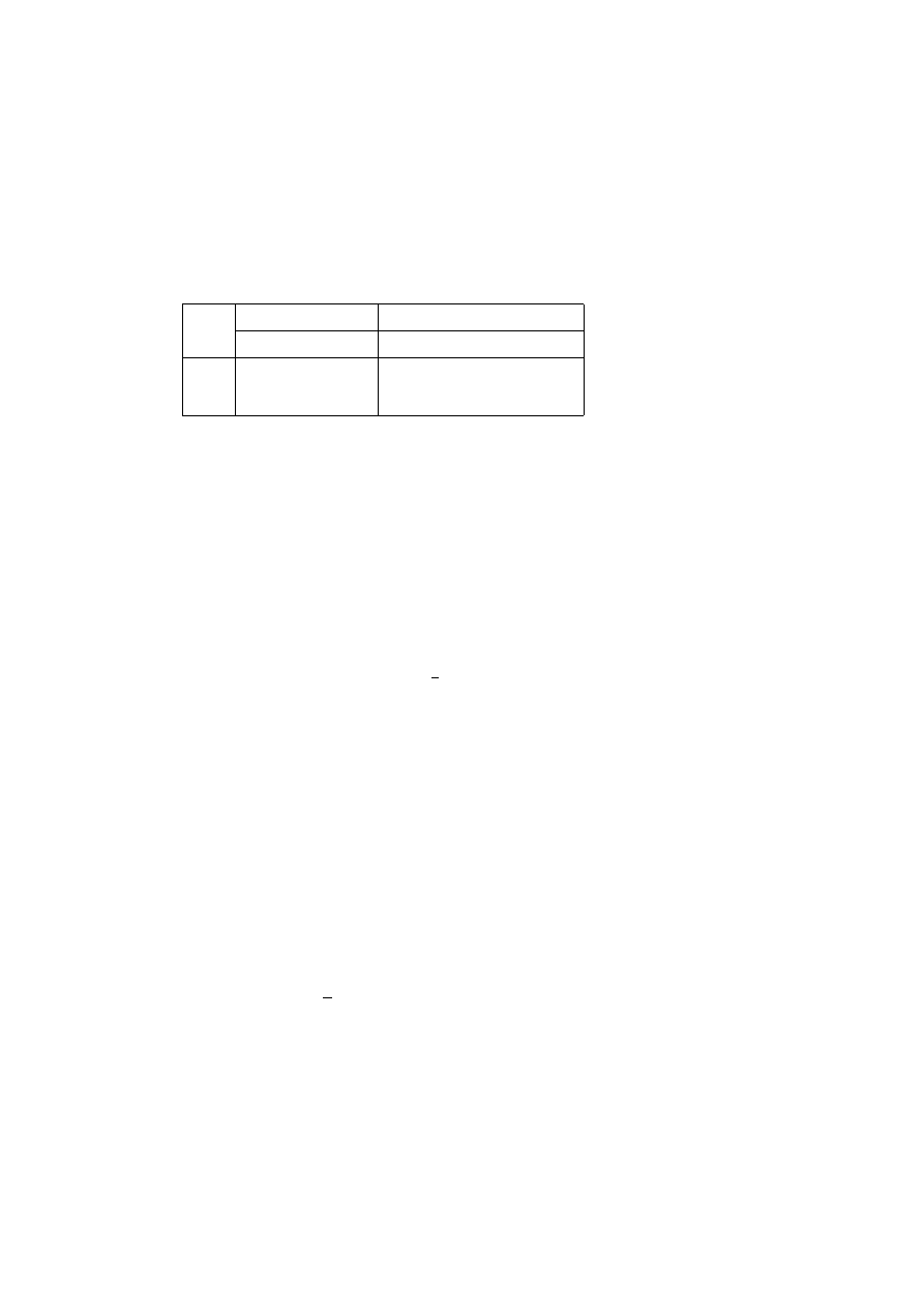
64
5
SPECIAL ASPECTS OF THE MATRIX FORMALISM
by the formula
cos ϕ = (±tr(W) − 1)/2.
(5.2.1)
The
+ sign is used for rotations, the − sign for rotoinversions.
One can list this correlation in a table
det(W) = +1
det(W) = −1
tr(W)
3
2
1
0
−1 −3 −2 −1 0
1
type
1
6
4
3
2
¯1
¯6
¯4
¯3 ¯2 = m
order
1
6
4
3
2
2
6
4
6
2
.
By this table the type of operation may be found, as far as it is determined by the
matrix part. For example, one takes from the table that a specific operation is a
two–fold rotation but one does not know if the operation is a rotatation or a screw
rotation, what the direction of the rotation axis is and where it is located in space.
This characterization will be done in the following list for the crystallographic
symmetry operations.
1. Type 1 or ¯
1:
no preferred direction
1 identity (for w
= o) or translation for w 6= o.
The coefficients of w are the coefficients of the translation vector.
¯1 inversion,
coordinates of the inversion centre F
x
F
=
1
2
w.
(5.2.2)
2. All other symmetry operations have a preferred axis (the rotation or rotoin-
version axis). The direction u of this axis may be determined from the equa-
tion
W u
= ±u.
(5.2.3)
The
+ sign is for rotations, the − sign for rotoinversions.
For type m, reflections or glide reflections, u is the direction of the normal
of the (glide) reflection plane.
3. If W is the matrix of a rotation of order k or of a reflection (k
= 2), then
W
k
= I, and one determines the intrinsic translation part, also called screw
part or glide part t/k by
(W, w)
k
= (W
k
, W
k−1
w
+ W
k−2
w
+ . . . + W w + w) = (I, t)
(5.2.4)
to t/k
=
1
k
(W
k−1
+ W
k−2
+ . . . + W + I) w.
(5.2.5)

5.2
The geometric meaning of (
W
,
w
)
65
The vector with the column of coefficients t/k is called the screw or glide
vector. This vector is invariant under the symmetry operation: W t/k
= t/k:
Indeed, multiplication with W permutes only the terms on the right side of
equation 5.2.5. Thus, the screw vector of a screw rotation is parallel to the
screw axis. The glide vector of a glide reflection is left invariant for the same
reason. Therefore, it is parallel to the glide plane.
If t = o holds, then (W, w) describes a rotation or reflection. For t
6= o, (W, w)
describes a screw rotation or glide reflection. One forms the so–called re-
duced operation by subtracting the intrinsic translation part t/k from (W, w):
(I, −t/k)(W, w) = (W, w − t/k) = (W, w
lp
).
(5.2.6)
The column w
lp
= w − t/k is called the location part because it determines
the position of the rotation or screw–rotation axis or of the reflection or
glide–reflection plane in space.
If W is a diagonal matrix, i. e. if only the coefficients W
ii
are non–zero, then
either is W
ii
= +1 and w
i
is a screw or glide component, or W
ii
= −1 and
w
i
is a location component. If W is not a diagonal matrix, then the location
part w
lp
has to be calculated according to equation 5.2.6.
4. The fixed points are obtained by solving the equation
W x
F
+ w = x
F
.
(5.2.7)
Equation (5.2.7) has a unique solution for all rotoinversions (including ¯
1,
excluding ¯
2 = m). There is a 1–dimensional set of solutions for rotations
(the rotation axis) and a 2–dimensional set of solutions for reflections (the
mirror plane). For screw rotations and glide reflections, there are no solu-
tions: there are no fixed points. However, a solution is found for the reduced
operation, i. e. after subtraction of the intrinsic translation part, by equation
5.2.8
Wx
F
+ w
lp
= x
F
.
(5.2.8)
The formulae of this section enable the user to find the geometric contents of any
symmetry operation. In reality, IT A have provided the necessary information for
all symmetry operations which are listed in the plane–group or space–group tables.
The entries of the General position are numbered. The geometric meaning of these
entries is listed under the same number in the block Symmetry operations in the
tables of IT A. The explanation of the symbols for the symmetry operations is
found in Sections 2.9 and 11.2 of IT A.
The section shall be closed with an exercise.

66
5
SPECIAL ASPECTS OF THE MATRIX FORMALISM
Problem 2B. Symmetry described by matrix–column pairs
.
For the solution, see p. 76.
The matrix–column pairs (A, a), (B, b) (C, c) and (D, d) have been listed or derived
in Problem 2A, p. 49, which dealt with their combination and reversion.
Question
(viii) Determine the geometric meaning of the matrix–column pairs
(A, a), (B, b), (C, c) and (D, d).
5.3
Coordinate transformations
There are several reasons to change the coordinate system. Some examples for
such reasons are the following:
1. If one and the same crystal structure is described in different coordinate
systems by different authors, then the structural data e. g. lattice parameters,
atomic coordinates, or displacement parameters (thermal parameters) have
to be transformed to the same coordinate system in order to be comparable.
The same holds for the comparison of related crystal structures.
2. In phase transitions frequently the phases are related by their symmetries,
e. g. in phase transitions of the second order. Often the conventional setting
of the new phase is different from that of the original one. Then a change
of the coordinate system may be necessary in order to find the structural
changes which are connected with the phase transition.
3. In the physics of macroscopic crystals (thermal expansion, dielectric con-
stant, elasticity, piezoelectricity, etc.) the properties are described mostly
relative to an orthonormal basis. Therefore, for physical calculations the di-
rection and Miller indices etc. have to be transformed from the conventional
crystallographic to an orthonormal basis.
4. In IT A, 44 space–group types are described in more than one conventional
coordinate system. The transition from one description to the other may be
necessary and needs coordinate transformations.
For these and other reasons either the origin or the basis of the coordinate system
or both may have to be changed. The necessary tools for these manipulations are
developed in this section.
5.3.1
Origin shift
At first the consequences of an origin shift are considered. We start from Fig. 1.4.1
on p. 11 where O is the origin with the zero column o as coordinates, and X is
a point with coordinate column x. The new origin is O
0
with coordinate column
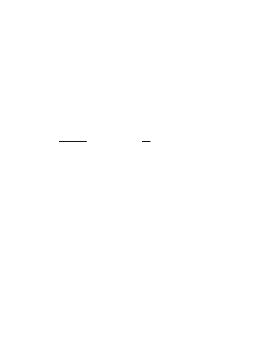
5.3
Coordinate transformations
67
(referred to the old origin) o
0
= p, whereas x
0
are the coordinates of X with respect
to the new origin O
0
. This nomenclature is consistent with that of IT A, see Section
5.1 of IT A.
For the columns, p
+ x
0
= x holds, or
x
0
= x − p.
(5.3.1)
This can be written in the formalism of matrix–column pairs as
x
0
= (I, −p) x or x
0
= (I, p)
−1
x.
(5.3.2)
[It may look strange to write the simple equation (5.3.1) in the complicated form
of (5.3.2). The reason will become apparent later in this section].
Equation (5.3.2) can be written in augmented matrices
x
0
=
P
−1
x
with
P
=
1 0 0 p
1
0 1 0 p
2
0 0 1 p
2
0 0 0
1
.
A distance vector
r
=
r
1
r
2
r
3
0
is not changed by
the transformation
r
0
=
P
−1
r
because the column p is not effective, see Sections
4.3 and 4.4.
How do the matrix and column parts of an isometry change if the origin is shifted ?
In the old coordinate system
˜x = (W, w) x holds, in the new one is ˜x
0
= (W
0
, w
0
) x
0
.
By application of equation (5.3.2) one obtains
(I, p)
−1
˜x = (W
0
, w
0
) (I, p)
−1
x
or
˜x = (I, p)(W
0
, w
0
)(I, p)
−1
x.
Comparison with
˜x = (W, w)x yields
(I, p)(W
0
, w
0
)(I, p)
−1
= (W, w) or
(W
0
, w
0
) = (I, p)
−1
(W, w)(I, p).
(5.3.3)
This means for the matrix and column parts of the pair
(W
0
, w
0
)
W’
= W, w
0
= w + Wp − p or w
0
= w + (W − I) p.
(5.3.4)
Conclusion. A change of origin does not change the matrix part of an isometry.
The change of the column w does not only depend on the shift p of the origin, but
also on the matrix part W.
How is a screw or glide component changed by an origin shift, i. e. what happens
if one replaces in
(W, w)
k
of equation 5.2.4 the column w by w
0
= w+(W −I) p ?
The answer is simple: the additional term
(W
k−1
+ W
k−2
+ . . . + W + I) (W − I) p does not contribute because
(W
k−1
+ W
k−2
+ . . . + W + I) W = (W
k−1
+ W
k−2
+ . . . + W + I) I.

68
5
SPECIAL ASPECTS OF THE MATRIX FORMALISM
An origin shift does not change the screw or glide component of a symmetry op-
eration. The component
(W − I) p is the component of p which is vertical to the
screw–rotation or rotation axis or to the mirror or glide plane. It causes only a
change of the location part w
lp
of the symmetry operation.
5.3.2
Change of basis
A change of basis is mostly described by a
(3 × 3) matrix P by which the new
basis vectors are given as linear combinations of the old basis vectors:
(a
0
1
,
a
0
2
,
a
0
3
) = (a
1
,
a
2
,
a
3
)P or (a
0
)
T
= (a)
T
P.
(5.3.5)
For a point X, the vector
−→
OX= x is
x = a
1
x
1
+ a
2
x
2
+ a
3
x
3
= a
0
1
x
0
1
+ a
0
2
x
0
2
+ a
0
3
x
0
3
or
x = (a)
T
x
= (a
0
)
T
x
0
.
By inserting equation (5.3.5) one obtains
x = (a)
T
x
= (a)
T
P x
0
or
x
= P x
0
,
i. e.
x
0
= P
−1
x
= (P, o)
−1
x.
(5.3.6)
The transformation of an isometry follows from equation (5.3.6)
and from the relation
˜x
0
= (W
0
, w
0
)x
0
by comparison with
˜x = (W, w)x:
(P, o)
−1
˜x = (W
0
, w
0
)(P, o)
−1
x or
˜x = (P, o)(W
0
, w
0
)(P, o)
−1
x
→
(W, w) = (P, o)(W
0
, w
0
)(P, o)
−1
or
(W
0
, w
0
) = (P, o)
−1
(W, w)(P, o).
(5.3.7)
From this follows
W
0
= P
−1
W P and w
0
= P
−1
w.
(5.3.8)
Example
In Fig. 1.5.2 on p. 13 the conventional and a primitive basis are defined for a
plane group of the rectangular crystal system. If
(a)
T
is the conventional,
(a
0
)
T
the
primitive basis, then
P =
1/2 1/2
−1/2 1/2
. One finds P
−1
=
1 ¯1
1 1
either by trial and error or
with equation (2.6.1) on p. 28.
For the coordinates, x
0
= P
−1
x or x
0
= x−y, y
0
= x+y holds. The conventional
coordinates 1, 0 of the endpoint of a become 1, 1 in the primitive basis; those of the
endpoint 1/2, 1/2 of b
0
become 0, 1; those of the endpoint 0, 1 of b become
−1, 1.

5.3
Coordinate transformations
69
If the endpoints of the lattice–translation vectors of Fig. 1.5.2 on p. 13, and those of
their integer linear combinations are marked with points, a point lattice is obtained.
Suppose, the origin is in the upper left corner of the unit cell of Fig. 1.5.2. Then,
the reflection through the line ‘a’ is described by the matrix–column pair
(W
1
, w
1
) =
1 0
0 ¯1
,
0
0
;
the reflection through the parallel line through the endpoint of the vector
b
0
is described by
(W
2
, w
2
) =
1 0
0 ¯1
,
0
1
.
Then, W
0
1
=
1 ¯1
1 1
1 0
0 ¯1
1/2 1/2
−1/2 1/2
=
0 1
1 0
.
The column w
0
1
is the o column because w
1
is the o column. According to equation
(5.3.8),
the column w
0
2
is obtained from w
2
by w
0
2
=
1 ¯1
1 1
0
1
=
¯1
1
.
Indeed, this is the image of the origin, expressed in the new basis. All these results
agree with the geometric view.
5.3.3
General coordinate transformations
In general both the origin and the basis have to be changed. One can do this in two
different steps. Because the origin shift p is referred to the old basis
(a)
T
, it has to
be performed first:
x
0
= (P, o)
−1
(I, p)
−1
x
= ((I, p)(P, o))
−1
x
= (P, p)
−1
x,
(5.3.9)
using
((I, p)(P, o))
−1
= (P, o)
−1
(I, p)
−1
.
In the usual way one concludes from equation (5.3.9) together with
˜x = (W, w) x and ˜x
0
= (W
0
, w
0
) x
0
:
(P, p)
−1
˜x = (W
0
, w
0
) (P, p)
−1
x or
˜x = (P, p)(W
0
, w
0
)(P, p)
−1
x.
Finally,
(W
0
, w
0
) = (P, p)
−1
(W, w) (P, p) is obtained, i. e.
(5.3.10)
W
0
= P
−1
W P and w
0
= −P
−1
p
+ P
−1
w
+ P
−1
W p.
(5.3.11)
The second equation may be written
w
0
= P
−1
(w + (W − I)p).
(5.3.12)
From equation 5.3.11 one obtains the equations (5.3.4) and (5.3.8) as special cases.

70
5
SPECIAL ASPECTS OF THE MATRIX FORMALISM
In
(4 × 4) matrices the equation (5.3.10) is written
(with
(P, p)
−1
→
P
−1
, (W, w) →
W
and
(P, p) →
P
)
W
0
=
P
−1
WP
.
(5.3.13)
This shape of equation (5.3.10 ) facilitates the formulation but not the actual cal-
culation. For the latter, the forms 5.3.11 or 5.3.12 are more appropriate.
ppppppppppppppppppppp
ppppppppppppppppppppppppppppppppppppppppppppppppppppppppppp
ppppppppppppppppppppp
ppppppppppppppppppppppppppppppppppppppppppppppppppppppppppp
ppppppppppppppppppppp
ppppppppppppppppppppppppppppppppppppppppppppppppppppppppppp
ppppppppppppppppppppp
ppppppppppppppppppppppppppppppppppppppppppppppppppppppppppp
pppppppppppppppp
pppppppppppppppppppppppppppppppppppppppp
pppppppppppppppppppppppppppppppppppppppppp
pppppppppppppp
pppppppppppppppp
pppppppppppppppppppppppppppppppppppppppp
pppppppppppppppppppppppppppppppppppppppppp
pppppppppppppp
(W,w)
(P,p)
.........
.....
....
....
....
..................
....................................
˜x
point
old coordinates
new coordinates
(W
0
, w
0
)
(P,p)
˜x
0
x
x
0
X
e
X
image point
Fig. 5.3.3 Diagram of ‘mapping of mappings’.
The formalism of transformations can be displayed by the diagram of Fig. 5.3.3.
The points X (left) and e
X (right) are represented by the original coordinates x und
˜x (top) and the new coordinates x
0
und
˜x
0
(bottom). At the arrows the corresponding
transformations are denoted. They describe from left to right a mapping, from
top to bottom the change of coordinates. Equation 5.3.10 is read from the figure
immediately: On the one hand one reads
˜x
0
= (W
0
, w
0
)x
0
along the lower edge;
on the other hand taking the way up
→ left → down one finds
˜x
0
= (P, p)
−1
˜x = (P, p)
−1
(W, w)x = (P, p)
−1
(W, w)(P, p)x
0
.
Both ways start at the same point and end at the same point. Therefore, the one way
can be equated to the other, and herewith equation 5.3.10 is derived in a visual way.
Remark. If there are different listings of the same crystal structure or of a set of
related crystal structures, it is often not sufficient to transform the data to the same
coordinate system. Even after such a transformation the coordinates of the atoms
may be incomparable. The reason is the following:
In IT A for each (general or special) Position the full set of representatives
(W, w
◦
)
is listed, see the table in Section 4.6. After insertion of the actual coordinates one
has a set of triplets of numbers, 24 (including the centring) in the table of Section
4.6. Any one of these representatives may be chosen to describe the structure in a
listing; the others can be generated from the selected one. The following Problem

5.3
Coordinate transformations
71
shows that different choices happen in reality. For a comparison of the structures
it is then necessary to choose for the description corresponding atoms in the struc-
tures to be compared.
Problem 3. Change of the coordinate system.
For the solution, see p. 77.
In R. W. G. Wyckoff, Crystal structures, vol. II, Ch. VIII, one finds the important
mineral zircon ZrSiO
4
and a description of its crystal structure under (VIII, a 4)
on text p. 5, table p. 9 and Figure VIII A, 4. Many rare-earth phosphates, arsen-
ates and vanadates belong to the same structure type. They are famous for their
interesting magnetic properties.
Structural data: Space group I
4
1
/amd = D
19
4h
, No. 141;
lattice parameters a = 6.60 ˚
A; c = 5.88 ˚
A.
The origin choice is not stated explicitly. However, Wyckoff’s Crystal Structures
started to appear in 1948, when there was one conventional origin only (the later
ORIGIN CHOICE 1, i. e. Origin at ¯
4m2).
Zr : (a)
0, 0, 0; 0,
1
2
,
1
4
;
1
2
, 0,
3
4
;
1
2
,
1
2
,
1
2
;
Si :
(b)
0, 0,
1
2
; 0,
1
2
,
3
4
;
1
2
, 0,
1
4
;
1
2
,
1
2
, 0;
O : (h)
(0, u, v; 0, ¯
u, v; u, 0, ¯
v; ¯
u, 0, ¯
v; 0,
1
2
+ u,
1
4
− v; 0,
1
2
− u,
1
4
− v;
¯
u,
1
2
, v +
1
4
; u,
1
2
, v +
1
4
; ) [ and the same with (
1
2
,
1
2
,
1
2
)+ ].
The parameters u and v are listed with u = 0.20 and v = 0.34.
In the Structure Reports, vol. 22, (1958), p. 314 one finds:
‘a = 6.6164(5) ˚
A, c = 6.0150(5) ˚
A’
‘Atomic parameters. Origin at centre (
2/m) at 0, ¯
1
4
,
1
8
from ¯
4m2.’
‘Oxygen: (
0, y, z) with y = 0.067, z = 0.198.’
In order to compare the different data, the parameters of Wyckoff’s book are to be
transformed to ‘origin at centre 2/m’, i. e. ORIGIN CHOICE 2.
Questions
(i) What are the new coordinates of the Zr atoms ?
(ii) What are the new coordinates of the Si atoms ?
(iii) What are the new coordinates of the O atom at
0, u, v ?
(iv) What are the new coordinates of the other O atoms ?
For a physical problem it is advantageous to refer the crystal structure onto a prim-
itive cell with origin in 2/m. The choice of the new basis is
a
0
= a; b
0
= b; c
0
=
1
2
(a + b + c).

72
5
SPECIAL ASPECTS OF THE MATRIX FORMALISM
Questions
(v) What are the new coordinates of the first Zr atom ?
(vi) What are the new coordinates of the first Si atom ?
(vii) What are the new coordinates of the O atom originally at 0,u, v ?

73
6
Solution of the exercises
6.1
Solution of problem 1
Solution 1A. Symmetry of the square.
For the problems, see p. 39.
Answers
(i) The symmetry operations of the square are:
(a) the mapping 1
−→ 1, 2 −→ 2, 3 −→ 3 and 4 −→ 4;
(b) the mapping 1
−→ 3, 2 −→ 4, 3 −→ 1 and 4 −→ 2;
(c) the mapping 1
−→ 2, 2 −→ 3, 3 −→ 4 and 4 −→ 1;
(d) the mapping 1
−→ 4, 2 −→ 1, 3 −→ 2 and 4 −→ 3;
(e) the mapping 1
−→ 2, 2 −→ 1, 3 −→ 4 and 4 −→ 3;
(f) the mapping 1
−→ 4, 2 −→ 3, 3 −→ 2 and 4 −→ 1;
(g) the mapping 1
−→ 3, 3 −→ 1, which maps the points 2 and 4 onto
themselves (leaves them invariant);
(h) the mapping 2
−→ 4, 4 −→ 2, which maps the points 1 and 3 onto
themselves (leaves them invariant).
(ii) The symmetry operations are, respectively:
(a) the identity operation 1,
(b) the two-fold rotation 2,
(c) the four-fold rotation 4 =
4
+
(anti-clockwise),
(d) the four-fold rotation
4
3
= 4
−1
= 4
−
(clockwise),
(e) the reflection m
x
in the line m
x
,
(f) the reflection m
y
in the line m
y
,
(g) the reflection m
+
in the line m
+
,
(h) and the reflection m
−
in the line m
−
.
(iii) The orders of these symmetry operations are, respectively:
1, 2, 4, 4, 2, 2, 2 and 2.
(iv) There are altogether eight symmetry operations.
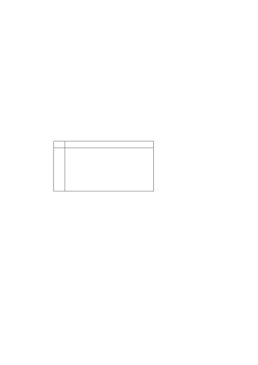
74
6
SOLUTION OF THE EXERCISES
Solution 1B. Symmetry of the square.
For the problems, see p. 63.
Answers
(v) The determination of the matrix–column pairs is particularly easy because
the origin O is a fixed point under all symmetry operations of the square.
Therefore, for all of them w = o holds. The images of the coordinate points
1, 0 and 0, 1 and their coordinates are easily found visually. The matrices
are:
1 =
1 0
0 1
,
2 =
¯1 0
0 ¯1
, 4
+
=
0 ¯1
1 0
,
4
−
=
0 1
¯1 0
,
m
x
=
¯1 0
0 1
, m
y
=
1 0
0 ¯1
, m
+
=
0 ¯1
¯1 0
, m
−
=
0 1
1 0
.
(vi) The multiplication table of the group of the square is
1
2
4
4
−1
m
x
m
+
m
y
m
−
1
1
2
4
4
−1
m
x
m
+
m
y
m
−
2
2
1
4
−1
4
m
y
m
−
m
x
m
+
4
4
4
−1
2
1
m
+
m
y
m
−
m
x
4
−1
4
−1
4
1
2
m
−
m
x
m
+
m
y
m
x
m
x
m
y
m
−
m
+
1
4
−1
2
4
m
+
m
+
m
−
m
x
m
y
4
1
4
−1
2
m
y
m
y
m
x
m
+
m
−
2
4
1
4
−1
m
−
m
−
m
+
m
y
m
x
4
−1
2
4
1
.
Remarkable properties of the multiplication table are
1. If there is a ‘1’ in the main diagonal of the table, then the element is the unit
element or has order 2 and vice versa. This is easy to see.
2. One finds that in each row and in each column each element of the group
occurs exactly once. This is a property of the multiplication table of any
group. It is not difficult to prove but the proof needs elementary group theory.

6.2
Solution of problem 2
75
6.2
Solution of problem 2
Solution 2A. Symmetry described by matrices.
For the problems, see p. 75.
Answers
(i) (B, b)(A, a): B A =
1 0 0
0 0 ¯1
0 1 0
, B a =
1/2
1/2
1/2
,
B a + b = B a for b = o.
Therefore, (B A, B a + b) = (C, c) =
1 0 0
0 0 ¯1
0 1 0
,
1/2
1/2
1/2
.
(ii) Analogously one calculates
(A, a) (B, b) = (D, d) =
0 0 1
0 1 0
¯1 0 0
,
1/2
1/2
1/2
.
(iii) (A, a)
−1
=
0 1 0
1 0 0
0 0 ¯1
,
−1/2
−1/2
1/2
.
(iv) (B, b)
−1
=
0 0 1
1 0 0
0 1 0
,
0
0
0
.
(v) (C, c)
−1
=
1 0 0
0 0 1
0 ¯1 0
,
−1/2
−1/2
1/2
.
(vi) (D, d)
−1
=
0 0 ¯1
0 1 0
1 0 0
,
1/2
−1/2
−1/2
.
(vii)
(B, b)
−1
(A, a)
−1
=
0 0 ¯1
0 1 0
1 0 0
,
1/2
−1/2
−1/2
= (D, d)
−1
6= (C, c)
−1
.
Note, that (B, b)
−1
(A, a)
−1
= [(A, a) (B, b)]
−1
= (D, d)
−1
.

76
6
SOLUTION OF THE EXERCISES
Solution 2B. Symmetry described by matrices.
For the problem, see p. 66.
Answer
(viii) We follow the procedure described in Section 5.2.
From the matrix parts the ‘types’ of the
operations are determined by the deter-
minants and traces:
A
B
C
D
det
+1 +1 +1 +1
tr
¯1
0
1
1
type
2
3
4
4
All the matrices are those
of rotations. The directions
[u v w] of the rotation axes
are determined by applying
equation (5.2.3):
A
B
C
D
u = v
u = v
u = u
u = w
v = u
v = w v = −w v = v
w = −w w = u w = v
w = −u
[1 1 0]
[1 1 1]
[1 0 0]
[0 1 0]
It is more or less a matter of taste and experience if one continues with
the calculation of the screw part (possibly o) by equation 5.2.5 or if one
calculates the (possibly non–existing) fixed points by equation 5.2.7. If the
order of the matrix is low then the calculation of the screw part is not so
costly as if the order is high. If the screw part turns out to be o or if there are
no fixed points then the calculation was not quite in vain because one then
knows that the other way will be successful.
‘Obviously’ the pair (B, b) describes a rotation because the column w
= o
indicates the origin O to be a fixed point. Solution: (B, b) describes a 3–fold
rotation with rotation axis [1 1 1] and the points x, x, x (including 0, 0, 0) as
fixed points.
We decide to calculate the screw parts in all other cases. Because of the order
2, the calculation for (A, a) is short. The pairs (C, c) and (D, D) cannot have
fixed points because in both cases a ‘
+1’ in the main diagonal is combined
with a non-zero coefficient w
i
in the column. This w
i
is a screw coefficient,
see the remark on diagonal matrices in Section 5.2. We start with (A, a).
1
2
0 1 0
1 0 0
0 0 ¯1
+
1 0 0
0 1 0
0 0 1
1/2
1/2
1/2
=
1
2
1 1 0
1 1 0
0 0 0
1/2
1/2
1/2
=
1/2
1/2
0
is the screw part of (A, a).
The reduced operation is
(A, a
lp
) =
0 1 0
1 0 0
0 0 ¯1
,
0
0
1/2
.
Equation 5.2.8 yields y
F
= x
F
, x
F
= y
F
,
−z
F
+ 1/2 = z
F
and the fixed
points x, x,
1/4, with arbitrary x. The fixed points are not really fixed points

6.3
Solution of problem 3
77
of the symmetry operation but are the coordinates of the screw–rotation axis
2
1
.
The calculation for (C, c) is a bit more lengthy:
t
4
=
1
4
1 0 0
0 0 1
0 ¯1 0
+
1 0 0
0 ¯1 0
0 0 ¯1
+
1 0 0
0 0 ¯1
0 1 0
+
1 0 0
0 1 0
0 0 1
1/2
1/2
1/2
=
=
1
4
4 0 0
0 0 0
0 0 0
1/2
1/2
1/2
=
1/2
0
0
.
The symmetry operation is a 4–fold screw rotation with HM symbol
4
2
.
The points of the screw axis are determined by equation 5.2.8 again:
x
F
= x
F
,
−z
F
+ 1/2 = y
F
, y
F
+ 1/2 = z
F
result in x,
0, 1/2 with
arbitrary x.
Analogously one determines (D, d) to describe a 4–fold screw rotation
4
2
,
the screw axis in
1/2, y, 0, with arbitrary y.
6.3
Solution of problem 3
Solution 3. Change of the coordinate system.
For the problem, see p. 71.
The new origin O
0
has the coordinates p
= 0, ¯
1
4
,
1
8
referred to the present origin
O. Therefore, the change of coordinates consists of subtracting 0,¯
1
4
,
1
8
from the old
values, i. e. leave the x coordinate unchanged, add
1
4
= 0.25 to the y coordinate,
and subtract
1
8
= 0.125 from the z coordinate.
Answers
The new coordinates are
(i) Zr
: (a) 0,
1
4
, ¯
1
8
∼
7
8
; 0,
3
4
,
1
8
;
1
2
,
1
4
,
5
8
;
1
2
,
3
4
,
3
8
;
(ii) Si
: (b) 0,
1
4
,
3
8
; 0,
3
4
,
5
8
;
1
2
,
1
4
,
1
8
;
1
2
,
3
4
, ¯
1
8
∼
7
8
;
(iii) O
: (h) 0, 0.20 + 0.25, 0.34 − 0.125 = 0, 0.45, 0.215.
This oxygen atom is obviously not the one (0, 0.067, 0.198) listed by the
Structure Reports but must be a symmetrically equivalent one. Therefore,
it is necessary to determine also the new coordinates of the other oxygen
atoms.

78
6
SOLUTION OF THE EXERCISES
(iv) O
: (h) The coordinates of the other oxygen atoms are (normalized 0 ≤
x
i
< 1):
0, 0.05, 0.215 0.20, 0.25, 0.535 0.80, 0.25, 0.535
0, 0.95, 0.785
0, 0.55, 0.785 0.80, 0.75, 0.465 0.20, 0.75, 0.465, all also with
(
1
2
,
1
2
,
1
2
) + .
The first one of these oxygen atoms corresponds to the one representing the
results of the later refinement with higher accurancy. The Si
− O distance is
reduced from 1.62 ˚
A to 1.61 ˚
A.
Answers
The change of basis to the primitive cell is described by the matrix
P
=
1 0 1/2
0 1 1/2
0 0 1/2
.
One determines the inverse matrix P
−1
=
1 0 ¯1
0 1 ¯1
0 0 2
,
by which the coordinates are transformed using the formula (5.3.6):
x
0
= P
−1
x. The coordinates x are those referred to the origin in
2/m.
(v) The new coordinates of the first Zr atom are
0 −
7
8
,
1
4
−
7
8
, 2 ·
7
8
∼
1
8
,
3
8
,
3
4
.
(vi) The new coordinates of the first Si atom are
0 −
3
8
,
1
4
−
3
8
, 2 ·
3
8
∼
5
8
,
7
8
,
3
4
.
(vii) The new coordinates of the first O atom are
0 − 0.215, 0.45 − 0.215, 2 · 0.215 ∼ 0.785, 0.235, 0.430.

Index
absolute value of a vector, 8
affine mapping, 17
affine space, 6
angle
calculation of, 16, 30
angle of rotation, 63
associative, 8, 24, 48
augmented column, 50
augmented matrix, 50
axis
of rotation, 32, 64
of rotoinversion, 33, 64
basis, 9
conventional, 14
orthonormal, 12
primitive, 13, 36
basis vectors, 10
Cartesian coordinates, 7
centre of inversion, 33
centred lattice, 13
coefficients of a vector, 10
column index, 21
column matrix, 21
column, augmented, 50
commutative, 8, 12, 24
conventional basis, 14
coordinate axes, 5
coordinate system, 5
coordinate transformation, 7, 66, 70
coordinates
Cartesian, 7
parallel, 6, 7
crystal class, 38
crystal pattern, 12
crystallographic symmetry operation,
64
dependent, linearly, 9
determinant, 25, 63
diagonal matrix, 21
dimension, 9
distance
calculation of, 15, 16, 30
distributive, 12, 24
Euclidean space, 6
finite group, 37
fixed point, 32, 65
fundamental matrix, 29
general position, 56, 57
glide part, 64
glide plane, 33
glide reflection, 33, 36, 65
glide vector, 34, 65
group
finite, 37
infinite, 37
order of a, 37
Hermann–Mauguin symbol, 35
HM symbol, 35
identity, 32, 49, 64
image, 17
improper isometry, 32
independent, linearly, 9
indices notation, 24
infinite group, 37
integer matrix, 21, 53
intrinsic translation part, 64, 65
inverse matrix, 28
inversion, 33, 35, 64
centre of, 33, 64
isometric mapping, 18
isometry, 18, 32
first kind, 18, 32
improper, 32
order of, 34
79

80
INDEX
proper, 32
second kind, 32
IT A, 4
lattice
centred, 13
primitive, 14
lattice basis, 13
primitive, 13
lattice parameters, 14
lattice vector, 13
law
associative, 8
commutative, 8, 12
distributive, 12
law of composition, 47
length of a vector, 8
linear combination, 10
linearly dependent, 9
linearly independent, 9
location part, 65
mapping, 17
affine, 17
isometric, 18
non–singular, 48
regular, 48
matrix, 21
augmented, 50
diagonal, 21
fundamental, 29
integer, 21, 53
inverse, 28
orthogonal, 28
rational, 21
regular, 26
singular, 26
symmetric, 21
transposed, 21
unit, 21
matrix notation, 20
matrix product, 24
matrix–column pair, 25, 46
mirror plane, 33
motion, 18
rigid, 18
multiplication table, 63
N –fold, 35
non–singular mapping, 48
O–matrix, 21
o–vector, 8
orbit of points, 57
order of a group, 37
order of an isometry, 34
origin, 5
orthogonal matrix, 28
orthonormal basis, 12
parallel coordinates, 6, 7
parallelogram of forces, 8
point group, 34, 40, 42
point lattice, 69
point orbit, 57
point space, 5
position
general, 56, 57
special, 58
primitive basis, 13
primitive lattice, 14
primitive lattice basis, 13, 36
product of matrices, 24
projection, 17, 48
proper isometry, 32
rational matrix, 21
reduced operation, 65
reflection, 33, 35, 65
reflection plane, 33
regular mapping, 48
regular matrix, 26
reverse operation, 48
rigid motion, 18
rotation, 32, 35, 63, 65
rotation angle, 33, 63
rotation axis, 32, 64
rotoinversion, 33, 35, 45, 63

INDEX
81
rotoinversion axis, 33, 64
row index, 21
row matrix, 21
scalar product, 6, 11
screw axis, 33
screw part, 64
screw rotation, 33, 36, 65
screw vector, 33, 36, 65
Seitz notation, 46
singular matrix, 26
site symmetry, 34
space
affine, 6
point, 5
vector, 8
space group, 34, 40
space–group type, 40, 55
special position, 58
square matrix, 21
subgroup, 37
symbol, Hermann–Mauguin, 35
symmetric matrix, 21
symmetry, 18
symmetry element, 42
symmetry operation, 18, 42
crystallographic, 18, 64
symmorphic, 42
trace, 63
translation, 12, 18, 32, 64
translation part, intrinsic, 64, 65
translation vector, 12, 32
transposed matrix, 21
type of space groups, 40, 55
unit cell, 30
unit matrix, 21
unit vector, 8
vector, 8
length of, 8
translation, 12, 32
unit, 8
vector coefficients, 10
vector lattice, 13
vector space, 8
volume of the unit cell, 30
Wyszukiwarka
Podobne podstrony:
Exact and Broken Symmetries in Particle Physics
Gray R M Toeplitz and Circulant Matrices
Gray R Toeplitz and circulant matrices A review (NOW, 2006)(ISBN 1933019239)(98s) MAl (1)
Gray R M Toeplitz and circulant matrices a review (web draft, 2005)(89s) MAl
CONCEPTUALIZING AND MAPPING GEOCULTURAL SPACE
Wick s Theorem for non symmetric normal ordered products and contractions
Crystal structure and properties of the copper(II) complex of sodium monensin A
Crystals, gems and psionics
Classical Symmetries and Conservation Laws
Magnea U , Lectures on random matrix theory and symmetric spaces
From Mapping Stories to the Narrative of Maps and Mapping
Serge Charbonneau Software Project Management A Mapping Between Rup And The Pmbok
Quantum Symmetry, The Cosmological Constant And Planck Scale Phenomenology
Groups, Symmetry And Fractals A Baker (2003) WW
Postmodernity and Postmodernism ppt May 2014(3)
Scoliosis and Kyphosis
L 3 Complex functions and Polynomials
więcej podobnych podstron