Chapter 3 - 1 - 4/18/2007

Chapter 3 – Basic graphics

This chapter focuses on simple ways to draw images on the screen.

NOTE: This chapter uses a function called scaleif.m which you can
download from the website. It will be explained in Chapter 8. Until
then, all you need to know is that it’s basically just used to scale
matrices.

Colormaps

So begin with the following lines:

>>img = 1:5;

You’ve done this before – it’s simply a vector of numbers going from 1 to 10
Then put up a figure window in matlab:

>>figure(1)

>> paintpots1 =[0 0 0
0.25 0.25 0.25
0.5 0.5 0.5
0.75 0.75 0.75
1 1 1]
>>colormap(paintpots1);

I’ll explain this colormap command in just a minute.
>>image(img)
The command image(img)draws a picture of the matrix

img

. In this case,

img

is a list of 5 numbers

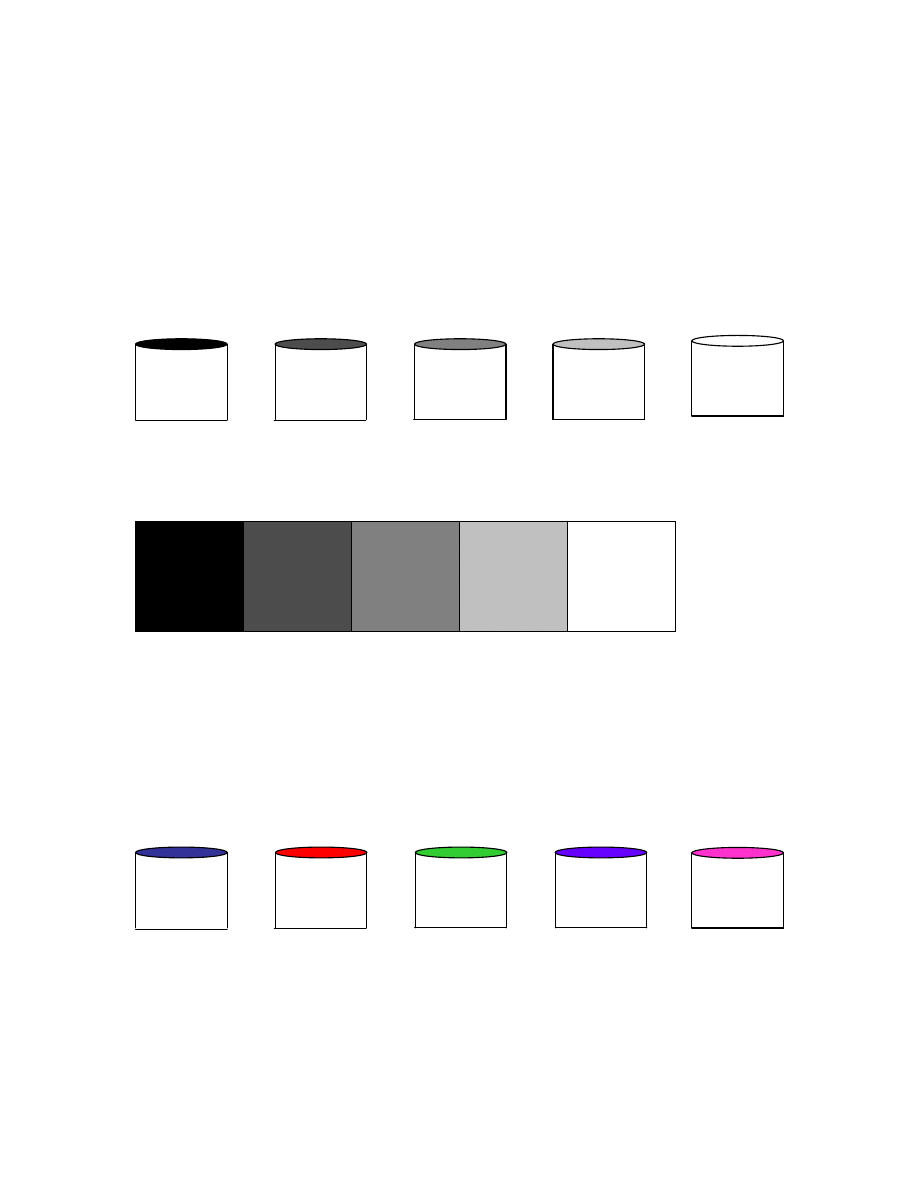
that is displayed as a row of vertical bars that gradually change in grayness as the value along the x-axis
changes from 1 to 5.

In image the rows go along the x-axis from left to right and the columns go along the y-axis from the top to
the bottom. So try this:

>>image(img’)

Now the bars will be horizontal and will increase in brightness as you go from the top to the bottom.

>>axis off
>>axis square

This will get rid of the axes

>>paintpots2=[0 0 1; 1 0 0; 0 1 0; 0.5 0 1; 1 0 1];
>>colormap(paintpots2)

Whoah! Why does the image suddenly change color?

Do you remember painting-by-numbers? 1 meant pink, 2 meant orange and so on.

img

basically creates an image like the paint-by-numbers image – with indices that will represent color 1, 2,

3, 4 and 5.

paintpots

represent two different sets of paints.

1 2 3

4

5

Chapter 3 - 2 - 4/18/2007

In

paintpots1

the values 1-5 was represented by different levels of gray. The command to tell Matlab

to paint the image img using paintpots1 was

colormap(paintpots1)

. Basically a

colormap

is a

mapping between a set of indices in an image (your paint-by-numbers picture) and a set of colors (your
picture). You may also hear the word palette to describe a colormap – the two words mean the same thing.

If you look at paintpots1 you will see that it is a 5x3 matrix.

>size(paintpots1)

The 5 rows refer to the fact that paintpots has five paint pots (indices into the colormap).
The 3 rows refer to the intensity of the red, green a blue gun. These gun intensities go between 0 (black)
and 1 (white).
>paintpots1
So the first paint pot contains black, the fifth paint pot contains white, and the intermediate ones contain
gradually lighter colors of gray.

This is why

>image(img)
>colormap(paintpots1)

produces an image that gradually goes from black to white.

Now lets look at paintpots2. Once again, paintpots2 represents 5 different colors.

>paintpots2

paintpots2 =
0 0 1

% only the blue gun, at maximum, this makes blue

1 0 0

% only the red gun, at maximum, this makes red

0 1 0

% only the green gun, at maximum, this makes green

0.5 0 1

% some red and lots of blue, makes purple

1 0 1

% red and blue, makes pink

So when you paint the img using this set of paintpots (a new colormap) the image changes.

1

2

3

4

5

1

2 3

4

5

1 2 3

4

5

Chapter 3 - 3 - 4/18/2007

One cute thing about Matlab is that it has a lot of pre-made
colormaps. Check out

>paintpots3=hot(5);
>colormap(paintpots3);
>paintpots4=hsv(5);
>colormap(paintpots4);

Also check out

winter, spring, cool, jet.

You can find a full list of Matlab colormaps using

>help graph3d

Spend some time playing with colormaps. For example, see if you can change a single row of a colormap.
For example if you want to replace purple with yellow:

>paintpots2b(4, :)=[1 1 0]

You should be able to guess what will happen if you use paintpots2b as your colormap.

Now see if you can remove all the red from paintpots1. If you have trouble, then you should look back at
chapter 2.

OK, now we are going to make a little m-file which will allow you to gradually change an image by changing
the colormap. So go to the menu bar and choose, File-> New ->M-file and save it in your MatlabClass/Misc
folder as LittleColormap.m

1
2
3
4
5
6
7
8
9
10
11
12
13
14
15
16
17
18
19

% UsingColormaps.m

%

% a little program that manipulates colormaps

%

% written by IF and GMB 3/2005

clear

all

close

all

img=1:10;

figure(1)

paintpots = ones(10,3);

colormap(paintpots)

image(img);

axis

off

;

for

i=1:10

paintpots (i,:)= (i/10);

colormap(paintpots);

pause

end

1 2 3

4

5

Chapter 3 - 4 - 4/18/2007

Lines 15-19. Ok, as you go from i = 1 to 10, you are gradually replacing the 1’s in paintpots with grays that
go from 0.1 (very dark) to 1 (white). Then you replace the old colormap with the new colormap, and
gradually the white in the image is replaced by grays. .

Line 18. The pause makes the program wait for a key press so you can observe each step.

OK, now we are going to replace lines 3-13 in

UsingColormaps.m

1
2
3
4
5
6
7
8
9
10
11
12
13
14
15
16
17
18
19
20
21

% % UsingColormaps.m

%

% a little program that manipulates colormaps

%

% written by IF and GMB 3/2005

clear

all

close

all

colormap(gray(256))

img = reshape(1:256,16,16);

image(img);

axis

square

axis

off

pause

for

i=1:200

paintpots = rand(256,3);

colormap(paintpots);

drawnow

end

I hope that was at least just a little bit exciting.

Line 12. The command reshape takes 3 arguments and allows you to reshape a vector or matrix into a
different shape. The first argument is the vector or matrix that you want to reshape. In this case we give
reshape a vector that goes [1 2 3 …256]. The second argument is the number of rows you want the new
matrix to have, and the second argument is the number of columns you want the new matrix to have. So in
this case reshape turns a 1x256 vector into a matrix with 16 rows and 16 columns. Of course this only works
because 16x16=256. Otherwise you would get the following error

>img = reshape(1:254,16,16);

??? Error using ==> reshape
To RESHAPE the number of elements must not change.

);

Take a look at img

>>img

Here’s another example of reshape where you take a 2x2 matrix and convert it into a 4 rows x 1 column
vector or a 1 x 4 vector

>tmp=[3 4 4 5 1 2; 6 7 1 2 2 3]
>tmp2=reshape(tmp, 3, 4)
>tmp3=reshape(tmp, 12, 1)

Now try the following:
Lines 13-15 simply draws the matrix img, removes the axis and makes the image square.
Lines 17-21. i will step from 1, 2, 3 …200. Each time, lines 18-20 will be executed. You remember how a

colormap

is like a collection of paint pots – with each paint pot having a number label. Here we have 256

paint pots, and the colors inside the paint pot are being assigned randomly.

rand(256,3)

creates a

256 x 3 matrix of random numbers. The random numbers vary between 0-1, so that allows us to define 256
random colors to go into the paint pots.

Chapter 3 - 5 - 4/18/2007

(A brief digression: if you type just the command

rand

then Matlab will just give you a single randomly

chosen number. Otherwise you have to describe the size of the matrix of random numbers that you want, as
is done here.)
Line 20. Tells Matlab to update the figure. Normally updating figures have a pretty low priority for Matlab,

drawnow

tells Matlab to put the other calculations on hold until it’s updated the figure.

Making a Gabor

Here we are going to use some of the things we have learned to make a Gabor filter. These are regularly
used for image processing. They are also popular as stimuli among vision scientists.

>sd=.3;
>x=linspace(-1,1,100);
>y=(1/sqrt(2*pi*sd)).*exp(-.5*((x/sd).^2));
>y=y./max(y);

So

y

is a 1-d Gaussian with a standard deviation of

sd=0.3.

It has a minimum value of 0 and a

maximum value of 1. We can

plot

this and see what it looks like.

>plot(x, y);

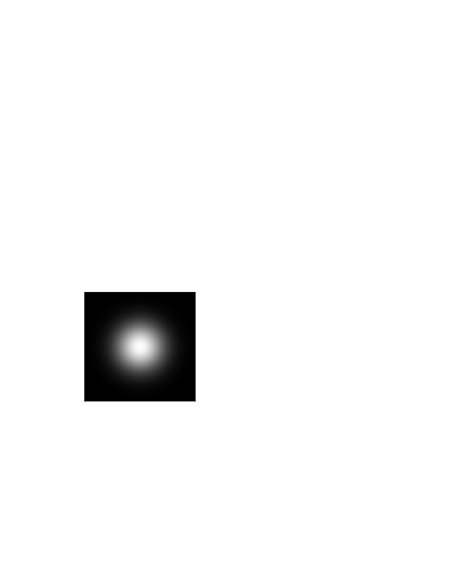
Now we use the outer product to create a two-dimensional Gaussian filter, with a maximum value of 1

>filt=(y'*y);
>max(filt(:))

And then we can look what that two dimensional Gaussian looks like. We are going to allow the colormap to
take 256 possible values of gray. That means we want filt to vary between 1 and 256.

>colormap(gray(256));
>scaled_filt=scaleif(filt, 1,256);
>image(scaled_filt)

10

20

30

40

50

60

70

80

90

100

10

20

30

40

50

60

70

80

90

100

We can then use this Gaussian window to filter any image we want. Let’s say we want to filter a sinusoidal
grating. We actually use much the same set of tricks.

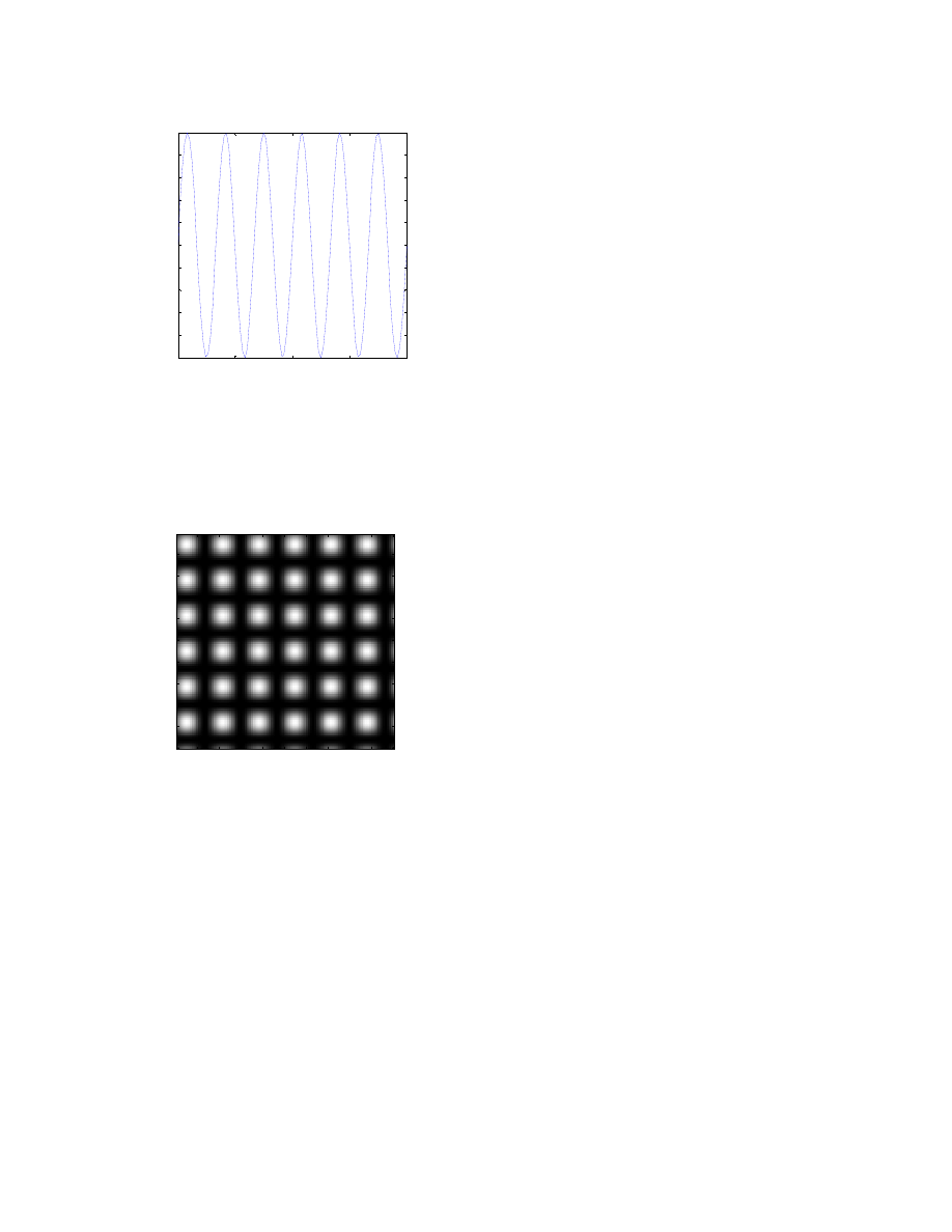
>sf=6;

% spatial freq in cycles per image

>y2=sin(x*pi*sf);

>y2=scaleif(y2, 0, 1);
>plot(x, y2);

Chapter 3 - 6 - 4/18/2007

-1

-0.5

0

0.5

1

0

0.1

0.2

0.3

0.4

0.5

0.6

0.7

0.8

0.9

1

This now gives us a 1-dimensional sinusoidal grating with a frequency of 6 cycles per image. We’ve scaled it
so it has a minimum value of 0 and a maximum value of 1. If we calculate the outer product of this sinusoid
with itself we get a weird checkerboard.

>img=(y2'*y2);
>colormap(gray(256))
>scaled_img=scaleif(img, 1, 256)
>image(scaled_img)

10

20

30

40

50

60

70

80

90

100

10

20

30

40

50

60

70

80

90

100

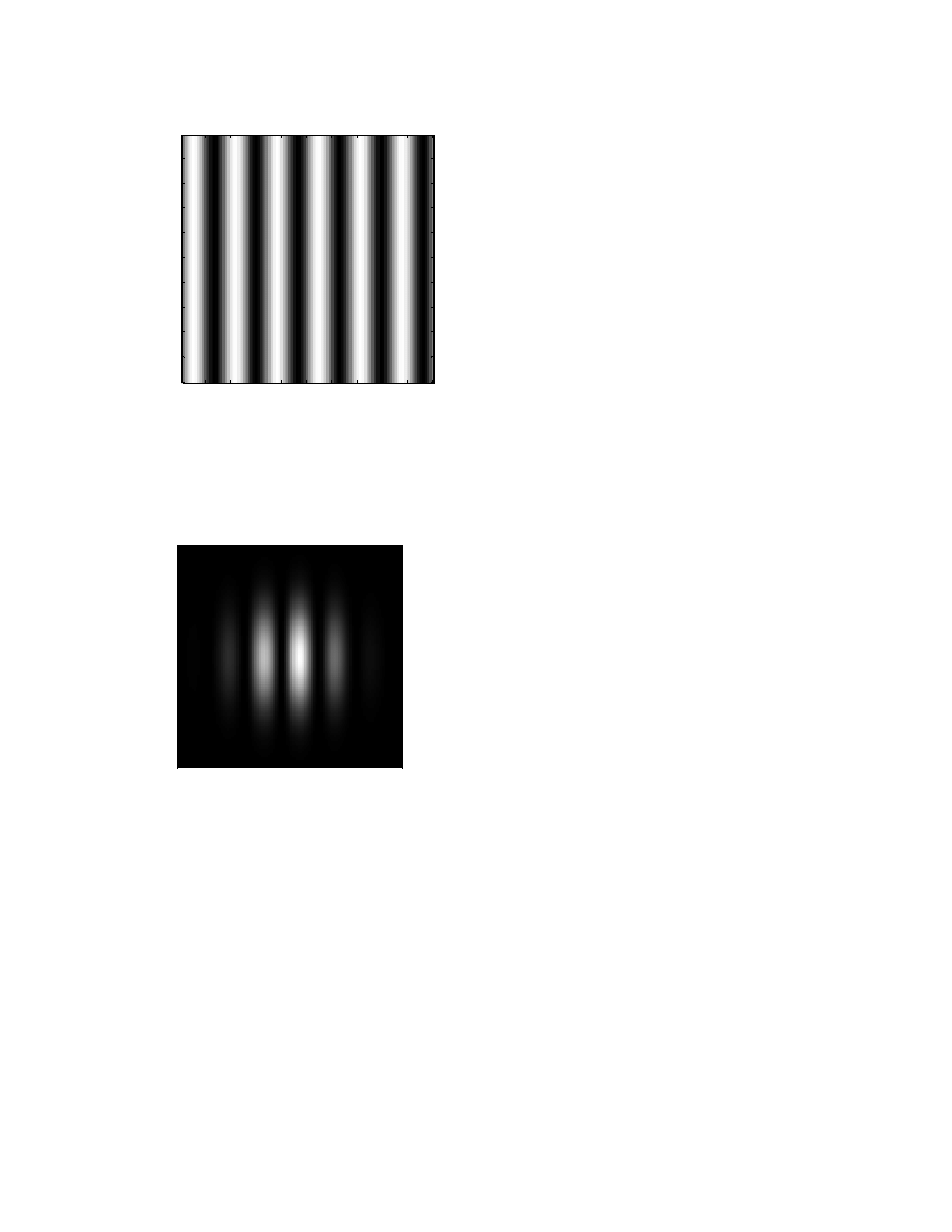
What we want to do is calculate the outer product of the one-dimensional sinusoid with a vector of ones.

y3=ones(size(y2));

img=(y3'*y2);

colormap(gray(256))

scaled_img=scaleif(img, 1, 256)

image(scaled_img)
Once again, img has a minimum of 0 and a maximum of 1

>max(img(:))

Chapter 3 - 7 - 4/18/2007

10

20

30

40

50

60

70

80

90

100

10

20

30

40

50

60

70

80

90

100

Now to create a Gabor (a sinusoid windowed by a Gaussian) becomes a piece of cake. We simply multiply
the two-dimensional Gaussian window by the two-dimensional Gabor.

>gabor=img.*filt;
>scaled_gabor=scaleif(gabor, 1, 256);
>colormap(gray(256))
>image(scaled_gabor);

10

20

30

40

50

60

70

80

90

100

10

20

30

40

50

60

70

80

90

100

Note that throughout this process we have worked with two versions of the Gaussian and the Gabor. The
original versions (

filt, img

) were scaled between 0 and 1. We did this to keep the nice property that

when the Gaussian filter was at its maximum, the brightness of the grating didn’t change, and when the
Gaussian filter was at 0 the Gabor was also at 0. But when we used

image

to look at these matrices we

converted them to range between 1-256 so as to match the colormap.

EXERCISES

1. Change

UsingColormaps.m

so that the squares flicker in shades of red only. Hint – you want the green

and blue monitor phosphors to always be at 0.
2. Make the image be 8x8 pixels instead of 16x16. That means that some of the
paint pots never get used.
3. Make the image be 20x20 instead of 16x16. This means that some of the paint pots will need to be used
twice. The following lines of code may help.

>x=1:40;
>x2=mod(x, 20)+1;

Chapter 3 - 8 - 4/18/2007

mod

finds the remainder of x/20, so it will vary between 0-19. If you add 1 this means that x2 varies

between 1-20.
4. Look at what happens to the matrices you made in ManipulatingMatrices.m when you use them as
images and play with the colormaps. Spend some time on this.
5. Change

UsingColormaps.m

so you create a figure where the squares alternate between red and blue. To

do this you are going to need to remember the things you learned in ManipulatingMatrices.m. You may also
find the command

mod

useful.

6. Create a horizontally oriented Gabor.