Against the Tide

Household Structure,

Opportunities, and Outcomes

among White and Minority Youth

Carolyn J. Hill

Harry J. Holzer

Henry Chen

2009

W.E. Upjohn Institute for Employment Research

Kalamazoo, Michigan

Library of Congress Cataloging-in-Publication Data

Hill, Carolyn J.
Against the tide : household structure, opportunities, and outcomes among white and
minority youth / Carolyn J. Hill, Harry J. Holzer, Henry Chen.
p. cm.
Includes bibliographical references.
ISBN-13: 978-0-88099-341-8 (pbk. : alk. paper)
ISBN-10: 0-88099-341-3 (pbk. : alk. paper)
ISBN-13: 978-0-88099-342-5 (hardcover : alk. paper)
ISBN-10: 0-88099-342-1 (hardcover : alk. paper)
1. Minority youth—United States. 2. Households—United States. 3. Discrimination
in employment—United States. I. Holzer, Harry J., 1957- II. Chen, Henry. III. Title.

HQ796.H4877 2009
306.85'608900973—dc22

2008052070

W.E. Upjohn Institute for Employment Research

300 S. Westnedge Avenue

Kalamazoo, Michigan 49007-4686

The facts presented in this study and the observations and viewpoints expressed are
the sole responsibility of the authors. They do not necessarily represent positions of
the W.E. Upjohn Institute for Employment Research.

Cover design by Alcorn Publication Design.
Index prepared by Diane Worden.
Printed in the United States of America.
Printed on recycled paper.

Contents

Acknowledgments

1 Introduction

Prior Research

Research Questions

Data and Methods

Outline of the Remainder of the Volume

Our Basic Findings

2 Outcomes for Young Adults in Two Cohorts

Sample

Outcome Measures

Limitations

Empirical Findings

Regression Analysis of Employment and Education Outcomes

Conclusion

3 Household Structure and Young Adult Outcomes

Sample and Measures

Estimated Equations

Empirical Results

Conclusion

4 Other Correlates of Household Structure and Their Effects

on Outcomes

Sample and Measures

Estimated Equations

Empirical Results

Conclusion

114

5 Conclusion

119

Summary of Empirical Findings

121

Implications for Further Research

125

Policy Implications

127

Appendix

139

References

155

The Authors

169

Index

171

About the Institute

181

Figures

3.1 Effects of Household Structure on Outcomes, without and

with Controls for Parental Income

4.1 Effects of Household Structure on Outcomes, without and

108

with Enrichment, Neighborhood, and Parenting Controls

Tables

2.1 Means on Employment Outcomes, by Gender and Race

2.2 Educational Attainment and Enrollment Status, by Gender

and Race

2.3 Means on Education Outcomes, by Gender and Race

2.4 Risky Behaviors: Substance Use and Unmarried Childbearing,

by Gender and Race

2.5 Means on Engagement in Risky Behaviors, by Gender and Race

2.6 Recursive Regressions Predicting Employment and

Education Outcomes

2.7 Recursive Regressions Predicting Employment and Education

Outcomes for Black Males and Females

3.1 Household Structure at Age 12, Total and by Race

3.2 Average Family Income for Various Household Structures,

Total and by Race

3.3 Household Structure at Age 12, by Mother’s

Educational Attainment

3.4 Effects of Household Structure on Outcomes, without and with

Controls for Parental Income

3.5 Effects of Race on Outcomes, without and with Controls for

Household Structure and Parental Income

3.6 Predicted Changes in Outcomes for Blacks over Time

(1960–1996) Due to Changes in Family Structure

3.7 Fixed-Effect Regressions with Controls for Mother’s Background

and Household Structure at Age 12

4.1 Means on Household and Parenting Characteristics by Household

Structure at Age 12

4.2 Effects of Household Structure on Outcomes: without and with

Neighborhood and Parenting Characteristics

vii

4.3 Joint Significance of Human Capital Enrichment, Parenting,

112

and Neighborhood Characteristics on Outcomes

A.1 Recursive Employment and Education Regressions for

140

Black Males

A.2 Recursive Employment and Education Regressions for

142

Black Females

A.3 Household Structure Stability of Respondents between Ages

144

2 and 12

A.4 Household Structure Stability of Respondents between Ages

145

12 and 16

A.5 Effects of Neighborhood and Parenting Characteristics on

146

Outcomes, with Household Structure at Age 12

viii

Acknowledgments

We would like to thank the Smith Richardson Foundation and the W.E.

Upjohn Institute for Employment Research for generous funding of the re-
search presented here. At the Upjohn Institute, Kevin Hollenbeck and three
anonymous referees gave us detailed comments that were very helpful as we
revised the manuscript. Seminar participants at the Bureau of Labor Statistics,
the Upjohn Institute, the Center on Law and Social Policy, and the Association
of Public Policy and Management (especially our discussant Greg Acs) gave
us very helpful comments as well. Igor Kheyfets provided excellent research
assistance. Finally, we want to thank Frank Furstenberg, who discussed our

ideas and findings with us at various stages of this research, providing his in-
sights along with his usual grace and good humor.

Introduction

Among young adults in the United States, employment and educa-

tional outcomes (such as wages, weeks worked, enrollment in college,
and educational attainment) are lower for minorities, and especially for
African Americans, than for whites. These gaps have been persistent
over time and in some cases are expanding. Among young black men,
employment outcomes are growing worse, falling behind even those of
young black women. High rates of crime and incarceration, and high
levels of teen pregnancy and unmarried parenthood, persist as well.

Why does a continuing gap exist between minority young adults—

especially black young adults—and their white counterparts, and why
are some gaps actually widening over time? One possibility involves
the increasing number of youth who have grown up in single-parent
households. The proportion of young blacks growing up in female-
headed households increased dramatically in the 1970s and 1980s; this,
in turn, might help explain why black male youth and young adults
today have experienced worsening employment outcomes, rising incar-
ceration, and increasing single parenthood.

In this monograph, we examine the effects of household structure

on young adults and how these effects might have contributed to some
of the negative trends we have observed for minorities (and especially
blacks) over time. We do not examine the causes of growing single
parenthood, especially in the black community. These causes likely in-
clude the many other causes of deteriorating employment outcomes and
high incarceration rates of less-educated men in general, and black men
in particular, as well as other factors (including many changes in social
norms, attitudes, and behaviors) that all limit young black males’ poten-
tial and their attractiveness as marriage partners. Understanding these
causes is crucial to developing any policy response that might attempt
to affect patterns of household formation. Still, for the purposes of this
study, we take the trends in household structure as a given and try to
better understand the effects of household structure on young people
growing up in these households.

2 Hill, Holzer, and Chen

While a large literature examines the effects of single parenthood

on children, it generally does not focus on different effects of single-
parent households by youth race and gender, nor does it tend to focus on
the extent to which different trends in education, employment, unmar-
ried childbearing, and crime across these groups might be attributable
to changes in household structure. The existing studies are also largely
based on data sources from the 1970s and 1980s rather than on more
recent data.

In addition to examining links between household structure and

outcomes, we hope to better understand the mechanisms or pathways
through which growing up in a single-parent household might affect
youth outcomes, and what other related factors might either reinforce
or counteract these effects. For instance, the children of single moth-
ers might be hurt by a loss of family income, a reduction in parental
supervision or contact time, a lack of productive male role modeling,
and other kinds of stress and instability associated with single-parent
families. Because of their lower income, children in single-parent fami-
lies are also more likely to live in poorer neighborhoods and attend
lower-quality schools.

On the other hand, perhaps the negative effects of single parent-

hood can be offset to some extent by better income supports, enrich-
ment activities in childhood, access to safer neighborhoods, more ef-
fective parenting practices on the part of the custodial parent, or by
positive involvement by the absent father or other family members. We
explore the extent to which some of these offsets are found in minority
and especially African American families, and whether they positively

influence both young males and young females in those families.

We use the National Longitudinal Survey of Youth (NLSY), and

particularly data from the 1997 cohort, to address these questions. This
survey collects a rich array of information about sample members, in-
cluding educational, employment, crime, and fertility outcomes, the
structure of households, and characteristics and behaviors of the youths’
parents. Furthermore, the survey collects information about a wide va-
riety of youths’ attitudes and engagement in risky behaviors, as well as
characteristics of their schools and neighborhoods.

Using the 1979 and 1997 cohorts of the NLSY, we first document

changes over time in outcomes related to education, employment, and
risky behaviors. We show summary data on additional outcomes avail-

Introduction 3

able in the NLSY97 and estimate regressions for select employment
and educational outcomes.

Next, we focus on data from the 1997 cohort and examine a wider

range of outcomes—including marriage, fertility, and incarceration—
and compute the extent to which differences in outcomes across racial
groups can be accounted for by differences in the household structures
under which children grew up, as well as differences in family income.
In addition to ordinary least squares (OLS) regressions, we estimate

individual and sibling fixed-effects models to explore whether effects
of household structure are likely causal.

Then we examine mediating variables through which single parent-

hood might affect youth outcomes, including parenting behaviors and
reduced supervision time or parental contact with youth. Other factors
that might be correlated with single parenthood—such as less stimu-
lating home environments and less stable or secure neighborhoods in
which young people reside—are considered here as well. Finally, we

sum up our findings and consider their broad implications for policy.

We find that young people growing up in single-parent families face

a combination of additional challenges that they must overcome in or-
der to succeed. In addition to lower family incomes, they grow up in
families with younger and less-educated mothers, in less stimulating
environments, and in less secure neighborhoods. Some of these factors
are likely caused, as least to some extent, by the single parenthood of
their mothers; others are not. It is as if these young people must swim
against the tide, facing fewer opportunities and many more challenges
than do most young people in two-parent families in order to attain
educational and employment success.

In this chapter we review previous literature on educational and em-

ployment outcomes among white and minority youth, and on household
structure and its effects on outcomes. We describe our data and empiri-

cal methods in greater detail, summarize our main findings, and, finally,
outline the remainder of the book.

4 Hill, Holzer, and Chen

PRIOR RESEARCH

Race/Gender Gaps in Outcomes: Education, Employment,
and More

A wide variety of literature documents the continuing gaps in em-

ployment between minorities—especially African Americans—and
whites, and within racial groups by gender. For example, employment
rates among young, less-educated minority women—particularly Af-
rican American single mothers—improved dramatically during the
1990s. These improvements are frequently attributed to the combina-
tion of a very strong economy, welfare reform, and increases in work
supports for low-income parents, such as the Earned Income Tax Credit
and child care subsidies (Blank 2002).

In contrast, employment rates among less-educated young white

and Hispanic men declined somewhat in the 1980s and stabilized in
the 1990s, while those of young black men continued to decline fairly
sharply throughout this period. A relatively large literature has explored
the causes of reduced employment among young black men, especially
in the 1980s. This literature has focused on the labor market chang-
es during that time that eliminated well-paying jobs for less-educated
men, as well as a number of factors that affected blacks more directly
than others.

In the 1990s, high rates of incarceration and more vigor-

ous child support enforcement seem to have further depressed the labor
market activity of this group (Holzer, Offner, and Sorensen 2005).

But why have these changes affected young black men so much

more than young black women or Hispanics? Employers seem much
more wary of hiring young black men than individuals from these other
groups when the jobs available do not require high levels of skill; thus
employers continue to discriminate in their hiring practices (Holzer
1996; Kirschenman and Neckerman 1991; Pager 2003).

But why these

factors might have worsened over time for young black men remains
unclear.

Changes in labor markets during the past two decades have raised

the rewards associated with educational attainment and cognitive skills
(Katz and Autor 1999), and differences in education and test scores ac-
count for large portions of the earnings gap between young whites and

Introduction 5

blacks.

The rate of high school completion nationally among young

blacks has apparently become comparable to that of young whites,
controlling for family background (Hauser 1997), but at least some of
this seems to be accounted for by General Educational Development
(GED) degrees, which are of lower economic value, rather than high
school diplomas.

Administrative data from school districts also sug-

gest much lower rates of high school completion than do self-report
surveys, though some controversy remains over which is more accu-
rate (Mishel and Roy 2006; Swanson 2004). Also, certain low-income
neighborhoods in major urban areas continue to have very high dropout

rates among young blacks (Orfield 2004). Rates of college attendance
and completion are lower for blacks relative to whites, perhaps because
of rising college costs and other factors (Ellwood and Kane 2000). Fur-
thermore, educational attainment among young Hispanics is consider-
ably lower than that of young whites, partly because of the presence of
immigrants among the former group.

In addition, a major gender gap in college enrollments favoring

women over men has developed among all ethnic groups, but especially
among young minorities (Jacob 2002; Offner 2002). And test score
gaps between young whites and minorities (despite some gains among
the latter in the 1980s) remain quite large and are not well understood
(Jencks and Phillips 1998). These gaps tend to appear quite early in life
(Fryer and Levitt 2004)—mostly before children enter kindergarten—

then widen in the first few years of school before stabilizing.

Other racial differences in social outcomes remain puzzling as well.

Why do so many more young black men participate in crime and be-
come incarcerated than do young people in any other race or gender
group? Freeman (1996) and Grogger (1997), among others, suggest that
declining wages and employment opportunities in the above-ground
economy help account for the decisions of less-educated young men to
engage in crime, though the sharp differences in criminal participation
by race and gender may not be fully attributable to this fact alone.

Similarly, the decline in marriage rates and the rise in out-of-

wedlock births among young blacks (and some Hispanics, such as
Puerto Ricans) have been noteworthy. Indeed, the rise in female head-
ship has been much steeper in black families than for other racial
groups (McLanahan and Casper 1995), and it appears at least partly
attributable to the declining employment and rising incarceration rates

6 Hill, Holzer, and Chen

observed among young men (Blau, Kahn, and Waldfogel 2000; Lichter

et al. 1992; Moffitt 2001; Wilson 1987), all of which tend to reduce
their marriageability.

Effects of Female Headship of Families: Blacks and Others

Has the fact that so many more young black men were growing

up in lower-income female-headed families over the past few decades
contributed to the greater decline in their employment and educational
prospects relative to virtually every other group?

The research evidence to date strongly suggests that growing up in

female-headed families appears to be harmful to youth outcomes such
as graduating from high school, gaining employment, and avoiding teen
pregnancy (Amato 2005; Haveman and Wolfe 1995; Hoffman, Foster,
and Furstenberg 1993; Maynard 1996; McLanahan 1997; McLanahan

and Sandefur 1994). Complementary findings suggest that growing up
in families with married parents has positive effects on youth (Thomas

and Sawhill 2002; Waite and Gallagher 2000). These findings have in-
spired a set of federally funded projects designed to explore the impacts
of healthy marriage promotion (Lerman 2002).

Are the effects of female headship for youth and young adults more

deleterious for blacks than for whites or Hispanics, or for black males
than for black females? The effects of female headship on young black
males might be more negative if, for example, their behaviors are more
negatively affected by a lack of parental supervision, or if their attitudes
and relationships are hurt by a lack of positive adult male role models
and mentorship in their lives.

But little of the earlier evidence on the topic suggests that this is the

case (Haurin 1992; Lee et al. 1994; McLanahan and Sandefur 1994),
though much of this work is based on data from the 1970s and 1980s.

In recent research, Page and Stevens (2005) find more negative effects
of divorce on young blacks than whites, at least partly because of lower
rates of remarriage among the former set of families. Dunifon and

Kowaleski-Jones (2002) find fewer negative effects of single parenthood
on young blacks than whites but more negative effects of cohabitation.
But even if the estimated impacts of female headship across race and
gender groups are comparable, the much greater frequency of single-
parenthood in the African American community might help account for

Introduction 7

some of the less positive outcomes and trends observed among blacks
in the 1980s and 1990s, especially among younger males.

Of course, the impacts of single parenthood—and the duration of

time in which families find themselves in this status—might depend
importantly on the extent to which the parents in these families are di-
vorced or never married. The presence of a second parent might affect
children quite differently, depending on whether the second parent is a
biological or a stepparent (Acs and Nelson 2003; Lansford et al. 2001).
Also, the traditional categories of being married, separated or divorced,
or remarried to a stepparent may be less relevant for many low-income
minority families than cohabitation: over time, single mothers seem to
cohabit with one or more biological fathers of their children, and with
varying frequency or duration.

Are the Effects of Household Structure Causal?

In all of this literature, questions have been raised about whether

these studies identify true causal effects of household structure. Esti-
mates of the negative impacts of teen pregnancy or single parenthood
and of the positive effects of marriage on both parents and children that
are based on ordinary least squares (OLS) regressions may be overstated
because they do not control for a set of unobserved characteristics of
these parents and families that are correlated with single parenthood but
not caused by it.

For instance, Geronimus and Korenman (1993) use comparisons

across female siblings to argue that the negative effects of teen parent-
hood are mostly due to unobserved factors, such as the poorer family
backgrounds of these young mothers. Rosenzweig and Wolpin (1993)

incorporate comparisons across cousins as well as siblings, and also find
smaller negative effects on the teen mothers and their children. Hotz,
McElroy, and Sanders (1996) look at pregnant teens who successfully
gave birth and compare their educational and employment outcomes to

those who miscarried; they generally find smaller negative effects as

well. Using sibling fixed-effects models (which control for unobserv-
able family characteristics) with data from the NLSY79, Sandefur and

Wells (1999) find that not living in a two-parent family was associated
with fewer years of education completed, suggesting a causal effect of
structure on educational attainment (though the magnitudes of effects

8 Hill, Holzer, and Chen

are modest). And Bronars and Grogger (1994), comparing mothers of
single children versus twins, suggest that some of the observed negative
effects on the education and incomes of unwed mothers are causal and
have long-term effects on black families.

The above studies mostly focus on the teen or unwed mothers them-

selves, rather than on the longer-term effects on children or youth of
growing up in a single-parent family. But Joyce, Kaestner, and Koren-
man (2000) and Korenman, Kaestner, and Joyce (2001) compare in-
tentional versus unintentional pregnancies, among other “natural ex-
periments,” to infer the effects of unwed parenthood on outcomes of
children in these families.

Though these researchers found that unwed

pregnant women smoke more and unwed mothers breast-feed less fre-
quently, few other negative impacts on children’s test scores or behavior
were observed. Similarly, Lang and Zagorsky (2001) use parental death

as an instrumental variable for parental absence and find relatively few
negative effects on child outcomes.

On the other hand, Gruber (2000) finds more negative effects on

child outcomes from laws making it easier for parents to divorce.

Vari-

ous studies using individual fixed effects (or “before-after” comparisons
for the same individuals) to analyze the impacts of divorce on children

frequently find negative effects (Morrison and Cherlin 1995; Page and
Stevens 2005; Painter and Levine 2000). Ananat and Michaels (2008)

use an instrumental variable strategy (with the gender of the first child

as the instrument) and find strongly positive causal effects of divorce

on child poverty as well, though Bedard and Deschênes (2005) find the
opposite with regards to mean income.

But individual fixed effects

will be of less value to the study of never-married mothers and their
children, as single parenthood is often a permanent characteristic of
these families.

While these studies raise important questions about potential biases

in OLS estimates, we do not believe they have settled the issue. For
instance, sibling studies have generally been based on small samples.
Other studies use instrumental variables that may have limited appli-
cability to the issue of children whose parents never married (such as
the Lang-Zagorsky measure of parental death), or that may be of low

quality (in terms of first-stage predictive power or true exogeneity). All
of these problems could lead to potential understatement of the size or

significance of the effects of growing up in a single-parent family.

Introduction 9

And, with a few exceptions (Dunifon and Kowaleski-Jones 2002; Page
and Stevens 2005), the above studies do not tend to focus on differences
in effects by race or gender.

Causal Pathways for Household Structure Effects

To the extent that growing up in a single-parent household has had

negative effects on young blacks in recent years, why do these occur?
What are the mediating variables through which these effects operate?
Many scholars have noted that family incomes are reduced in single-
parent families relative to two-parent families since the former have
only one earner; and lower family incomes clearly affect the school-
ing and behavioral success of children growing up in these families
(Duncan 2005). However, Mayer (1997) makes the case that other fac-
tors (such as parental attitudes and behaviors) that are heavily corre-
lated with low incomes might actually be more important direct sources
of problems for children growing up in poor families. In addition, the

time constraints of single working parents might make it more difficult
for them to interact with their children or to supervise their children’s
behavior and use of time. Financial and emotional stress on the mothers
might lead to poor parenting (Kalil et al. 1998), in terms of the mothers

meting out harsher punishments and getting into more conflicts with
their children (Carlson and McLanahan 2002). Less orderly households
might also result from these stresses on parents, which might affect chil-
dren and youth negatively as well (Dunifon, Duncan, and Brooks-Gunn
2001).

Instability in living arrangements and residential locations might

also contribute to poorer youth outcomes, as a stable environment
might be necessary for children to develop healthy relationships and to
maintain routines of productive activity (such as homework). The lower
incomes and instability of single-parent families might result in less
intellectually stimulating environments for children (Bradley, Caldwell,
and Rock 1988) or residence in less secure neighborhoods. In addition,
some of these factors might affect minority families more strongly than
whites, and males in these families more severely than females—es-
pecially given the absence of positive male role models and authority

figures in these families.

10 Hill, Holzer, and Chen

In one well-known attempt to disentangle the negative impacts of

single parenthood into these competing sources, McLanahan and Sand-
efur (1994) consider family income as well as “parenting variables”
(such as regularity of contact with the absent father, parental assistance
with homework or reading, degree of supervision and regulation of be-
havior, strictness of discipline, and positive aspirations) that are likely
to be at least somewhat correlated with single parenthood (because of a
single parent’s limited time and greater stress). They also consider the
frequency of residential mobility (as a measure of instability in family
life that is higher for single-parent families) and quality of peers and

schools. They find that lower income accounted for roughly half of the
poorer outcomes of youth observed in these families. Many of the par-
enting and mobility variables also contribute to worse youth outcomes,
though major racial and gender differences in these impacts were not
found.

In an analysis of parents and youth in lower-income neighborhoods

in Philadelphia, Furstenberg et al. (1999) focus on a similar set of par-
enting behaviors as well as various school and neighborhood factors
as determinants of youth outcomes. Using an analytical framework
that stresses the importance of youth development in the context of
the family’s school and community environment (Eccles et al. 1993;
Sameroff, Seifer, and Bartko 1997), Furstenberg et al. note that even
single parents in lower-income neighborhoods can encourage success
among youth by “managing risk and opportunity,” through either “pro-
motive” or “preventive” strategies (or both). The promotive strategies
include developing trust and healthy communication between parents
and children, encouraging greater youth autonomy and participation in
decision-making at home, and encouraging youth involvement in a va-
riety of school and community organizations that might strengthen their
cognitive, social, and psychological skills. In contrast, the preventive
strategies entail more restrictions on youth activity out of the home,
more supervision, and stronger punishments for violations of the rules.

The authors find that minority single parents and those in poorer

neighborhoods have fewer resources (of time, money, and information)
with which to pursue the promotive strategies, and therefore tend to fall

back on preventive measures to a greater extent. They find that both
sets of strategies can generate some successful outcomes among youth,
but that differences in these approaches can also account for some of

Introduction 11

the variations in outcomes observed between single- and two-parent
families, and between whites and minorities.

The study by Furstenberg and his colleagues focuses not only on

mediating factors through which single parenthood affects outcomes,
but also on a range of parental behaviors that can either offset or re-
inforce whatever disadvantages single-parent families have in income
levels and quality of school or neighborhood. The extent to which their

findings can be replicated in broader nationwide data, covering a much
wider range of youth outcomes in school and in the labor market, needs
to be examined.

The special developmental needs of young black males, and the

kinds of mentoring and education/training programs that address these
needs, have also received some attention (e.g., Mincy 1994). Clayton,
Mincy, and Blankenhorn (2003) have also recently focused on father-
hood among black men and have considered how more positive parent-
ing can be encouraged both within marriage and among black noncus-
todial fathers.

But the extent to which specific parenting behaviors

among noncustodial black fathers are associated with improved educa-
tional and employment outcomes among their sons and daughters has
not been explored systematically.

Preliminary Studies Using the NLSY97

The potential usefulness of the NLSY97 in addressing these many

questions is discussed below. But some new evidence on this topic, and
the richness of the data on youth and their families (even relative to the
earlier 1979 cohort of the NLSY and other data sets), was highlighted in
a volume of papers (Michael 2001) and in a special issue of the Journal
of Human Resources (JHR 2001). Using the NLSY97, the papers in
those volumes provide an early snapshot of young people aged 12–16,

and of the important influences of family background and environment
on their own attitudes and behaviors. In particular, Pierret (2001) found
strong effects of family structure on grades, tendency to use alcohol and
drugs, and participation in crime; Moore (2001) found similar effects
on adolescent sexual behavior, and Tepper (2001) found major effects
of parental regulations on adolescent use of time. At that point, though,
few data were available in the NLSY97 that allowed a study of the
determinants of educational and employment outcomes (instead of just

12 Hill, Holzer, and Chen

youths’ expectations of these outcomes), as well as marriage, fertility,
crime, and other outcomes.

Summary

A lengthy literature strongly suggests that single parenthood has

negative consequences for the educational, employment, and behav-
ioral outcomes of young people growing up in these households. But
many important questions remain unanswered. In particular, we still
know relatively little about the extent to which growing single parent-
hood among minorities, and especially among blacks, can help account
for poor educational, employment, marital, pregnancy, and crime out-
comes among young adults—and even among black males relative to
black females. The extent to which previous estimates of the impacts
of household structure on young adult educational and employment
outcomes are causal remains uncertain, as are the exact mechanisms
through which household structure might have its effects. Generating
answers to these questions can provide insight into developing appro-
priate policies to help young minorities improve their educational and
employment outcomes in the future.

RESEARCH QUESTIONS

In this monograph, we address the following questions:

1) What are the trends over time in employment, education, sin-

gle parenthood, and participation in risky behaviors for young
adults, overall and separately by race and gender?

2) What are the effects of growing up in a single-parent home on

outcomes related to education, employment, unmarried par-
enthood, and incarceration for young adults overall, as well as
separately for young black men and young black women? Has
the growth of single parenthood, especially female headship in
black families, contributed to growing gaps in education and
employment for black male youth and young adults relative
to other males, and to gaps between black males and black
females?

Introduction 13

3) Are the observed effects of growing up in a single-parent home

causal, or do the effects reflect other factors that are correlated
both with growing up in a single-parent home and with young-
adult outcomes?

4) To the extent that growing up in a single-parent home affects

youth and young-adult outcomes, why does it do so? Do its ef-
fects work primarily through reduced income or through other
parenting behaviors and instability? To what extent does it
work through quality of the home and neighborhood environ-
ment (which may or may not be causally related to single par-
enthood per se)? Do these patterns vary by race and gender?

DATA AND METHODS

To answer these questions, we analyze data from the National

Longitudinal Survey of Youth (NLSY). We focus on the 1997 cohort
(NLSY97), a nationally representative sample of about 9,000 youths
who were ages 12 to 16 at the end of December 1996. Our analysis

uses the first eight panels of data, allowing us to observe this cohort in
early adulthood (ages 20 to 24). To provide a comparative perspective
over time on our research questions, we also use an earlier cohort, the
NLSY79, a panel survey that has followed more than 12,000 young
men and women who were 14 to 21 years old at the end of 1978.

Using the extensive data available in the NLSY, we estimate the ef-

fects of growing up in a single-parent home on a wide variety of young-
adult outcomes, separately by race and gender. Although we focus on
the NLSY97 cohort, we generate estimates of outcomes using both the
1979 and 1997 cohorts to document changes over time for different
race-gender groups.

Our goal is to examine a wide variety of outcomes of youth and

young adults that might be affected by growing up with single parents.
As Acs (2006) notes, the range of outcomes potentially affected might
be grouped into three categories: cognitive, school-based, and behav-
ioral.

All of these outcomes might ultimately affect other measures of

individual success, especially earnings and employment.

14 Hill, Holzer, and Chen

The NLSY97 contains a wealth of information for measuring the

outcomes and explanatory measures in our study. As an overview,
these data provide detailed evidence on youths’ behaviors and attitudes
with regard to education, employment, marriage, fertility, sexual activ-
ity, criminal activity, and risky behaviors (e.g., the use of alcohol or
drugs).

The survey also includes extensive information on the youths’

living situations and parental characteristics, including education, in-
come, marital status, attitudes, and rule-setting behaviors (from the sur-

vey of a parent or parental figure in the first round of the survey, as well
as from the youth respondent).

With regard to educational outcomes of interest, the survey contains

information on enrollment status, level of schooling completed, grade
point averages, and scores on the Armed Services Vocational Aptitude
Battery (ASVAB).

With regard to employment outcomes of interest, information

is available about all spells of employment (as an employee, a self-
employed worker, or a freelancer) since the age of 12, and about the
wages and other characteristics of each job.

With regard to marriage, sexual behavior, and fertility, the survey

collects information on the dates of all sample members’ cohabiting re-
lationships, marriages, and disruptions or dissolution of these relation-
ships, and on the number of pregnancies, live, and nonlive births.

Finally, with regard to criminal outcomes and other risky behaviors,

the survey collects self-reported information on arrests and convictions
for various crimes, as well as use of alcohol, cigarettes, and drugs. It
can also gauge incarceration based on whether the interview in any par-
ticular year took place in a jail or prison facility.

The NLSY97 contains an equally rich supply of explanatory vari-

ables for these outcomes. In addition to key measures of race, ethnic-
ity, and gender for each sample member, a strength of the data set is
the availability of measures of family structure—our primary explana-
tory variable of interest—for the youth. We can distinguish whether
the sample member was in a household with both biological parents, a
single-parent household, or another type of family structure.

The survey contains extensive detail about other characteristics of

the youths’ parents, families, households, and nonresident relatives.
These characteristics, which include parents’ age, education, employ-
ment, and income, constitute a core set of explanatory control variables

Introduction 15

in our statistical models. Other measures of parental attitudes and be-
haviors, and of household characteristics, are included as mediators of
the effects of household structure, or as reinforcing or offsetting factors
of growing up in a single-parent household. Such information on pa-
rental child rearing actions and attitudes is gleaned through questions to

the parent respondent in the survey’s first round, as well as to the youth

respondent in the first and subsequent rounds.

The NLSY97 survey design restricted the sample universe for se-

lected survey questions, and we use some of these questions in our
analysis. For example, some questions about parenting behaviors and
relationships were only asked of youth who were 12 to 14 years old at
the end of December 1996. This sample restriction should not limit the
analysis in a meaningful way. As a whole, the NLSY97 contains rich
detail on youth outcomes, youth characteristics, family structure and
other characteristics, parental characteristics, and other aspects of the
youth’s environment for analyzing the research question of how family

structure influences a range of youth and young adult outcomes.

As for the empirical work and methods we will use, we first docu-

ment trends in education, employment, and other behavioral outcomes
by race and gender over the period of the 1980s and 1990s, using data
from the two NLSY cohorts. We will especially highlight continuing
gaps in outcomes by race and gender that appear in the most recent
NLSY data.

Then, using the NLSY97 data, we present estimates from reduced-

form equations for outcomes of interest related to education, employ-
ment, unwed parenthood, and incarceration. We focus on the effects
of household structure (measured at age 12) on these outcomes, con-
trolling for a number of sample member and maternal characteristics.
These equations are estimated without and then with controls for family
income, as this is one of the clearest mechanisms through which single
parenthood might affect observed outcomes for youth.

To deal with issues of causality and unobserved personal character-

istics, we estimate both individual and sibling fixed-effects models, in
which the former focus on changes over time in individual circumstances
while the latter focus on differences across sibling pairs. These methods
use smaller samples, limiting our ability to produce separate estimates
by youth race and gender.

Still, these models may produce something

closer to causal estimates of the effects of household structure.

16 Hill, Holzer, and Chen

We next explore how effects of household structure are mediated

through household and parental characteristics and behaviors. Follow-
ing McLanahan and Sandefur (1994), Furstenberg et al. (1999), and
others, we add a set of variables that may be correlated with household
structure. Such measures include the degree to which the home environ-

ment provides an “enriching environment” (defined as the home usu-
ally having a computer, usually having a dictionary, and whether the
youth take extra classes or lessons such as dance or music) or the qual-
ity of the neighborhood in which the youth and his or her family live.
We will also consider measures of parenting styles and quality (such
as parental knowledge of whom these young people spend time with
when not at home) or household stability and routine as other potential
mechanisms. Our goal in estimating these equations is to explore some

of the mediating factors that prior research has identified as potentially
important in accounting for the observed effects of household structure
on youth outcomes, or that might tend to offset or exacerbate those ef-
fects in various situations.

OUTLINE OF THE REMAINDER OF THE VOLUME

In Chapter 2, we document changes in both employment and edu-

cational outcomes between the 1979 and 1997 cohorts of the NLSY,
with a particular emphasis on how these trends differ across race and
gender groups. We also present summary data on engagement in risky
behaviors from both cohorts, but especially from the 1997 cohort. The
chapter concludes with results from a set of estimated recursive equa-
tions in which educational outcomes (in particular, dropping out of high
school) are related to a range of personal and behavioral characteris-
tics, all of which are then used to explain employment outcomes for
NLSY97 sample members in 2004–2005.

In Chapter 3, we begin our exploration of the effects of household

structure on youth outcomes, using the NLSY97 data only. We docu-
ment the differences in household structure that exist across race and
gender groups. We also consider associations between household struc-
ture, personal characteristics (such as maternal education), and family
income. We then present results from estimated reduced-form equa-

Introduction 17

tions in which the outcomes are estimated as functions of the household
structure of young people at age 12.

These estimates are provided for the entire sample, separately for

blacks, and further separately for black males and black females. The
equations for the entire sample are used to estimate the extent to which
differences in household structure across race and gender groups can
account for differences in employment, educational, and behavioral
outcomes across these groups. The separate equations for blacks and
for black males and females enable us to estimate how household struc-
ture might affect outcomes differently within these groups, and how it

might help account for group-specific trends over time.

In all three

cases, we also estimate equations without and with controls for fam-
ily income, to see the extent to which estimated impacts of household
structure might work through family income. Finally, we present some

estimates from individual and sibling fixed-effects models, to explore
the extent to which our estimates are truly causal.

In Chapter 4, we analyze correlations between household structure

and a number of other household characteristics, such as the following
three:

1) Parenting style (e.g., whether parents are strict or supportive,

how closely they monitor their children and are involved with
them, and how structured family activities are),

2) The richness of the home environment, including the presence

of computers or dictionaries and participation in various extra-
curricular activities,

3) The quality of the neighborhood, as measured either by the

survey respondent or by the surveyor.

We estimate reduced-form equations for employment, educational,

and behavioral outcomes as functions of household structure as well
as of these additional variables, to infer the extent to which the latter
can help either to account for estimated effects of the former or to rein-
force or offset these effects. These are also estimated for the sample as
a whole and separately by race and gender.

In Chapter 5, we review our findings and consider their implications

for policy and for further research.

18 Hill, Holzer, and Chen

OUR BASIC FINDINGS

The analyses in subsequent chapters find the following:

• Most young adults show positive trends in educational attainment

and employment over time, but a gap remains between young
blacks and Hispanics on the one hand and young whites on the
other for both sets of outcomes. Young blacks also have children
while unmarried and become incarcerated much more frequently
than white or Hispanic youth. Within each racial group, progress
has been greater for women than for men, and postsecondary
school enrollments are now greater for women than for men in
each racial group. Young black men, in particular, show the least
improvement in almost all outcomes. Among black high school
dropouts, the low rates of employment activity and high engage-
ment in crime and other risky behaviors are pronounced.

• About half of young people today grow up in households without

both biological parents, while about 80 percent of young blacks
do so. Growing up without both biological parents appears to
have modestly negative impacts on employment outcomes of
young adults and more pronounced negative impacts on educa-
tional attainment, unmarried parenthood, and incarceration. The
greater incidence of living with a single mother among blacks
accounts for substantial portions of the racial differences among
young adults in some outcomes, especially educational attain-
ment, and also helps to account for a relative lack of progress
(or even some deterioration) over time in these outcomes. The
employment and incarceration outcomes of young black men are
particularly strongly affected by growing up with a single mother.
The lower family incomes of single-parent families—especially
those headed by never-married mothers—account for some but

not all of these impacts. And there is some evidence (from fixed-
effects models) that these estimated negative effects of growing
up with a single parent are at least partly causal.

• The negative effects of growing up in families without both par-

ents are often compounded by the fact that these households tend
to provide less enrichment to children and frequently are located

Introduction 19

in dangerous neighborhoods. Parenting behaviors are also related
to household structure. Some of the parenting behaviors are likely
caused, at least to some extent, by single parenthood. However,
the human capital and neighborhood variables are more likely to
be additional determinants of outcomes that happen to be corre-
lated with structure, though the low family incomes and instabil-
ity to which single parenthood contributes probably reinforce the
observed gaps in these variables. Either way, these three sets of

additional variables have jointly significant effects on most of the
observed youth outcomes and can account for some substantial
parts of the observed effects of household structure on these out-
comes.

In short, youth and especially young minorities who grow up in

single-parent families face a range of difficulties and disadvantages in
terms of achieving academic or labor market success and staying out of

trouble. Some of these difficulties appear to be caused by the singleness
of their parents and some not. But in any case, they are truly swimming
against the tide as they mature into young adulthood and beyond, in that
they have less opportunity to succeed than their counterparts because of
a variety of disadvantages that they experience.

At the same time, our findings illuminate a variety of personal

and family characteristics that might be used to offset disadvantages
and promote positive outcomes for young people, especially those in
low-income and single-parent families. Sensible policies might seek to
promote a variety of circumstances, including healthy marriages, more
positive noncustodial fatherhood, higher incomes for working single
parents, better schooling or employment options and safer neighbor-
hoods for poor youth, and better child care and parenting among single
parents. All of these would promote opportunity and success among
otherwise disadvantaged youth. These broad approaches are explored
in the book’s concluding chapter.

20 Hill, Holzer, and Chen

Notes

1. The relative wages of less-educated young men were also declining during much

of this period, implying that reduced work incentives were at least part of the
reason for their diminishing work effort (Juhn 1992). Decreasing availability of
blue-collar and manufacturing jobs, rising skill demands, rising competition from
immigrants and women, “spatial mismatch” problems, and persistent discrimina-

tion have also likely contributed to the difficulties of young black men (Holzer
2000).

2. Ethnographic work suggests that employers perceive a stronger work ethic among

Hispanics, especially immigrants; while they perceive more negative attitudes
among young blacks and especially males (Wilson 1996). Fear of crime and vio-
lence, especially from those with criminal records, also appears to contribute to
the problem. There is some evidence that employers who do not conduct formal
criminal background checks engage in broad statistical discrimination against
young black men as they seek to avoid hiring exoffenders (Holzer, Offner, and
Sorensen 2005).

3. Johnson and Neal (1998) show that most of the black-white wage gap, but much

less of the employment gap, disappears after controlling for racial differences in
years of education and test scores. This evidence has been disputed by some au-
thors (e.g., Rodgers and Spriggs 1996).

4. Educational attainment as measured in the Current Population Survey (CPS) does

not carefully distinguish between GEDs and regular high school diplomas. For
evidence on the weaker value of GEDs in the labor market, see Cameron and
Heckman (1993).

5. See Ellwood and Jencks (2004) for a discussion about similarities and differences

in trends in marriage and childbearing between more- and less-educated women
over time. See also Edin and Kefalas (2005) for ethnographic evidence on the
importance of marriage for low-income young women, despite their feeling that

stable marriages might be unattainable, especially given the employment difficul-
ties and unproductive behaviors that they perceive among the young men in their
lives.

6. A number of authors (e.g., Graefe and Lichter 1999; Manning, Smock, and

Majumdar 2004; Wu and Wolfe. 2001) have noted a growing trend towards co-
habitation among unmarried parents in the United States, and that such unions
tend to be shorter and more unstable than traditional marriages. But the effects
of different patterns of cohabitation on youth outcomes, among both whites and
minorities, have only recently been explored (Acs and Nelson 2003; Brown 2002;
Dunifon and Kowaleski-Jones 2002; Manning and Lamb 2003).

7. Ashcraft and Lang (2006) discuss this literature and the potential upward and

downward biases in various estimates of these effects.

8. Korenman and his colleagues conduct a variety of tests, including a comparison

of siblings and cousins among children who were and were not born to single par-
ents, the addition of controls for whether the pregnancy was intended or mistimed,

Introduction 21

and instrumental variables (IVs) for the availability of abortion services and child
support enforcement at the state level, as exogenous predictors of unwed births.

9. See also Stevenson and Wolfers (2007).
10. See also Stevenson and Wolfers (2007) for a more skeptical view of the causal

effects of marriage and household structure on these outcomes.

11. Sigle-Rushton and McLanahan (2004) review these studies and the very mixed

nature of their findings. Ashcraft and Lang (2006) discuss various reasons these
studies might generate downward biases in estimates of negative effects associ-
ated with teen or unmarried childbearing.

12. See Mincy (1994) for a set of papers that focus on young black males in fatherless

families. Lee et al. (1994) find stronger effects of absent mothers on their daugh-
ters but less evidence of stronger effects of absent fathers on sons.

13. In related literature, Garfinkel et al. (1998) looks at the role of child support pay-

ments by noncustodial fathers, and Holzer, Offner, and Sorensen (2005) examine
the effects of child support enforcement on employment of young black men.

14. Similarly, Carneiro and Heckman (2003) note the importance of both cognitive

and noncognitive “skills” on employment outcomes.

15. Hotz and Scholz (2001) describe reports that compare administrative and survey

data reports on employment and income (especially for low-income populations);
Kornfeld and Bloom (1999) examine the reliability (or lack of measurement error)
of self-reported measures of earnings and employment; Abe (2001) and references
therein discuss self-reports of antisocial behaviors, including comparisons across
the NLSY79 and ’97 cohorts, and differences by race and gender; and Laumann et
al. (1994) discuss issues of reliability in survey questions about sexual behavior.
The results of these studies are quite mixed but suggest that self-reported risky or
illegal behaviors may be quite seriously underreported, relative to self-reported
measures of employment or education.

16. A number of measures of family process and parenting style using such questions

have been constructed by Child Trends (an independent, nonpartisan research cen-
ter), under contract with the U.S. Department of Labor. These variables are avail-

able in the public use file as “family process” variables, and a separate data file
appendix from Child Trends and the Center for Human Resource Research (1999)
assesses the data quality, internal consistency and reliability, construct validity,
and predictive validity.

17. We do not explore instrumental variable estimates because of our skepticism about

the usefulness of some of these models, as noted earlier in the chapter.

18. Throughout our work in this monograph, we will use Chow tests to examine the

statistical validity of pooling our estimates across race and gender groups as op-
posed to providing separate estimates for these groups.

Outcomes for Young

Adults in Two Cohorts

This chapter presents descriptive information about employment,

education, and risky behaviors for young adults in the mid-1980s and
the mid-2000s. In particular, we examine three areas: 1) employment
outcomes of hourly wages, hours worked, and weeks worked; 2) educa-
tional outcomes of enrollment, degrees attained, high school test scores,
and high school grade point averages (GPAs); and 3) engagement in
risky behaviors of early substance use, childbearing while unmarried,
and illegal activities. Simple descriptive statistics on these outcomes
are presented for the full sample (separately by cohort) as well as by
race and gender within each cohort. These statistics make it possible
to examine differences across groups within a cohort, trends for a spe-

cific group across cohorts, and differences across groups across cohorts.
Later in the chapter, we report descriptive statistics for additional out-
comes for the more recent cohort of young adults and present regression
estimates that show statistical relationships between their outcomes.
The chapter concludes with a summary of the trends in young adults’
outcomes over the past two decades.

SAMPLE

Our analysis in this chapter uses data from the 1979 and 1997 cohorts

of the National Longitudinal Survey of Youth (NLSY79 and NLSY97).
As we noted in Chapter 1, the NLSY79 is a nationally representative
survey of more than 12,000 youth ages 14 to 21 as of December 31,
1978; and the NLSY97 is a nationally representative survey of almost
9,000 youth ages 12 to 16 as of December 31, 1996. The NLSY79 co-
hort was surveyed annually until 1994 and biannually afterwards. The
NLSY97 cohort has been surveyed annually since 1997.

24 Hill, Holzer, and Chen

For descriptive analyses in the first part of this chapter, we impose

three sample restrictions. First, to examine young adults of the same
ages across the two cohorts (in Tables 2.1, 2.2, and 2.4), we include only
young adults who were ages 22 to 24 at the time they were interviewed
in either 1987 (for the early [NLSY79] cohort) or 2004–2005 (Round
8 for the later [NLSY97] cohort). These were the youngest members of
the NLSY79 cohort (born primarily between 1962 and 1964) and the
oldest members of the NLSY97 cohort (born primarily between 1980
and 1982). While all of these sample members were 22 to 24 at the
time they were interviewed, the NLSY79 sample members were slight-
ly older because the 1987 interviews were conducted mostly between
April and June, while the 2004–2005 interviews were conducted mostly
between November and January.

We focus on the 1987 and 2004–2005 interviews because the 12

months prior to these dates represent similar points in the business cy-
cle. While unemployment rates in late 1986–early 1987 were higher
than those in 2004 (about 7.1 versus 5.5 percent), labor market tightness
is comparable across the two years relative to most estimates of “full
employment” for those periods.

The labor market was recovering from

a steep recession in the former period and from a more modest down-
turn in the latter one.

For the second sample restriction, we include only the largest racial/

ethnic subgroups: white non-Hispanics, black non-Hispanics, and His-
panics. For the third sample restriction (a relatively minor one) we ex-
clude any persons who were still enrolled in high school and persons
who were enrolled in college for whom the type (two-year or four-year)
could not be reliably determined.

Regression analyses presented in the

last part of the chapter (as well as sample means in Tables 2.3 and 2.5)
are based on samples that include all ages of white, black, and Hispanic
sample members from the NLSY97 only.

Another notable characteristic of the sample used in the analyses is

that we include sample members who were incarcerated at the time of
the survey.

Incarcerated individuals account for about 2 percent (n = 69)

of our 22- to 24-year-old NLSY79 sample and 1.3 percent (n = 51) of
our NLSY97 sample, but nearly 6.5 percent (n = 29) of young black
men in the 1979 cohort and 6.2 percent (n = 33) of young black men in
the 1997 cohort. The Bureau of Justice Statistics reports that roughly 12
percent of young black men between the ages of 16 and 34 are now in-

Outcomes for Young Adults in Two Cohorts 25

carcerated at any one time, while about twice that number are on parole
or probation (Bureau of Justice Statistics 2007). Other analyses of this
population that do not include incarcerated individuals contribute to the
well-known undercount of young black men in census surveys (see,
for example, Bound 1986 and Stark 1999). Of course, labor market
outcomes of incarcerated individuals are predetermined, and including

these observations in an analysis may result in findings that are unrepre-
sentative of those who truly have choices to make. Thus, in addition to
the estimates presented here, a full set of estimates that do not include
incarcerated individuals is available from the authors on request. While
the magnitudes of some results change, virtually no qualitative result is
changed by the inclusion or omission of incarcerated individuals from
the sample.

OUTCOME MEASURES

This chapter examines three categories of outcomes for young

adults: employment, education, and risky behaviors.

For employment outcomes, we examine hourly wages, hours

worked, and weeks worked. Wages are measured at the time of the sur-
vey or in the most recent job prior to the survey date.

To achieve com-

parability across the two NLSY cohorts, the wage rate includes tips and

bonuses as well as regular wages. We adjust nominal wages for inflation
to 2005 dollars using the Consumer Price Index Research Series Using
Current Methods (CPI-U-RS), which is the Bureau of Labor Statistics’

most complete effort to measure inflation and eliminate upward biases
in the Consumer Price Index over time.

Hours and weeks worked are

measured for the 52 weeks prior to the week of the interview.

For educational outcomes, we examine enrollment and educational

attainment. We measure these variables in November for each cohort
(1986 for the NLSY79 and 2004 for the NLSY97).

First, we classi-

fy each respondent as either not enrolled or enrolled. If not enrolled,
we further classify the respondent by attainment: high school dropout
or GED,

high school diploma, some college or associate’s degree, or

bachelor’s degree or higher. If enrolled, we further classify the respon-
dent by type of school: two-year college (including vocational and

26 Hill, Holzer, and Chen

technical school) or four-year college or university (including graduate
school).

For the 1997 cohort, we also examine educational outcomes

of GPAs from high school transcripts as well as results from the Armed
Services Vocational Aptitude Battery (ASVAB) tests.

For risky behaviors and outcomes we examine measures from each

cohort of whether the sample member drank alcohol, smoked cigarettes,
or smoked marijuana before age 18; and whether she or he had a child
and was unmarried as of the survey date in 1987 or 2004–2005.

For

the 1997 cohort only, we examine whether the sample member had ever
engaged in illegal activities, been arrested, or been incarcerated.

The variables for drinking alcohol, smoking cigarettes, and smok-

ing marijuana before age 18 were all created in a similar way in both the
NLSY79 and NLSY97: With information about the sample member’s
birth date, as well as self-reported information about the date at which

the respondent first drank alcohol (or smoked a cigarette or marijuana),
we created binary variables indicating whether the sample member had
engaged in each activity before his or her eighteenth birthday.

To measure whether the sample member was unmarried with a child

by the time of the interview in 1987 or 2004–2005, we used informa-
tion from the fertility and relationship history taken in the 1987 round
of the NLSY79, and information about birth dates of sample members’
children in the NLSY97.

Engaging in illegal activity is measured with a series of self-

reported responses indicating whether the sample member in the
NLSY97 had ever been engaged (prior to the latest survey date) in
relatively less serious or less violent activity (for example, had ever
damaged property or stolen something worth more than $50), as well
as relatively more serious or more violent activity (for example, had
ever attacked someone, carried a handgun, or been arrested). We also
measure whether the sample member had ever been incarcerated, using
information on the place of residence at the time of the survey in each
year as well as self-reports of incarceration. The tendency for self-
reported crime and incarceration rates to understate actual rates may be
substantial, particularly for minorities (Hindelang, Hirschi, and Weis
1981). For this reason, we have constructed an incarceration rate based
at least partly on information that is independent of potentially biased
self-reported information.

Outcomes for Young Adults in Two Cohorts 27

LIMITATIONS

This chapter’s findings are characterized by limitations arising from

the time at which we observe young adults in the two cohorts, and from
their self-reports of risky behaviors and crime. First, the periods during
which we observe the two NLSY cohorts are not ideal for the purpose
of comparing behaviors and outcomes across time. As noted, to com-
pare young adults of the same ages at similar points in a business cycle,
we examine outcomes in 1986–1987 and 2004–2005. Yet real wages
of less-educated workers stagnated or declined over the period 1973–
1995, then rose thereafter. Thus, the time frame we examine combines

a period of modestly declining real wages with a period of significantly
rising real wages, masking the actual trend in earnings. Another timing
issue, noted earlier, is that interviews were conducted primarily from
April to June in 1987 and from November to January in 2004–2005.
Ideally, these survey months would be identical (or more similar) across
the survey cohorts and years.

Sample members’ self-reports of risky and criminal behaviors con-

stitute a second limitation of the analyses. Self-reports, especially of
risky behaviors or crime, may be underreported because of the stigma
associated with these actions. Self-reports of criminal activity may
be differentially underreported among blacks (Abe 2001; Hindelang,
Hirschi, and Weis 1981; Viscusi 1986). It may be, however, that the
stigma associated with these behaviors has fallen over time; we are not
aware of more recent research investigating this issue. Furthermore, the
dichotomous measure we use (whether the sample member engaged
in a particular activity) is a less precise measure of the activity than
a frequency measure would be. All in all, these measurement issues
likely bias the estimated relationships in our regressions towards zero

or insignificant results.

Our measure of incarceration, however, is less

likely to suffer from measurement error because it is based on both self-
reports and place of residence at the time of the survey.

In part because of these limitations, our regression estimates should

not be interpreted as showing causal effects. However, as most of the
biases noted above should not be more severe in one cohort or another
or in any particular race or gender group, these biases should not af-

28 Hill, Holzer, and Chen

fect the inferences we draw regarding trends over time and differences
across these groups.

EMPIRICAL FINDINGS

We first present descriptive statistics for employment and educa-

tional outcomes, then for risky behaviors, for young adults ages 22–24
in 1986–1987 and in 2004–2005. Next, focusing on the more recent
cohort, we present results from regression analyses predicting wages,
weeks worked, and high school dropout status.

Descriptive Statistics on Employment Outcomes

Table 2.1 presents descriptive statistics for employment outcomes

of hourly wages, hours worked, and weeks worked. These outcomes
are presented separately by cohort for the 22- to 24-year-old subsample,
and separately by race and gender within each cohort. In general, Table
2.1 shows (consistent with other studies) that males tend to earn more,
and work more hours and weeks, than do females; and that hourly wag-
es for blacks tend to be lower than for whites, as do hours and weeks
worked (where the difference is relatively larger).

With regard to trends across the cohorts, overall the results in Table

2.1 indicate that real wages and weeks worked each have grown about
7 percent.

The greatest gains in hours and weeks worked of any group

were experienced by black and Hispanic females. This growth has been
widely attributed to policy changes in the 1990s, primarily welfare re-
form and expansion of supports for low-income working parents such

as the Earned Income Tax Credit (EITC) and child care benefits (Blank
2002). In contrast, hours worked fell the most for white and black men

(though only the results for the latter are statistically significant). The
results for both groups are mostly driven by outcomes among the less
educated, as noted by Juhn (1992, 2000).

Despite these trends, many of the race and gender gaps observed

in the earlier cohort persist in the more recent one. Within each racial
group, women still have lower wages, hours worked, and weeks worked
than men,

though they exhibit greater improvement than men in al-

Outcomes for Young Adults in Two Cohorts 29

most all cases. These trends are consistent with prior research showing
that female labor force activity has grown more rapidly than that of
males for several decades (Juhn and Potter 2006) and in the 1980s cor-
responded with more rapid wage growth (Blau and Kahn 1997).

With regard to race gaps within gender, these data indicate that His-

panics have achieved greater parity with whites in labor market out-
comes in the later cohort than had been observed earlier, despite strong
immigration growth over this time period.

But black men have fallen

even further behind young white and Hispanic men in terms of hours

and weeks worked, a finding that remains even when incarcerated in-
dividuals are removed from the sample.

Some gain in relative wages

for black men compared to white men is observed: the gap between
the wages of white and black men shrank from 18 percent in 1987 to
14 percent in 2005. However, this pattern is likely driven by the with-
drawal of lower-wage workers from the labor force altogether (Chandra
2003), and thus is an artifact of the composition of the wage-earning
sample.

Table 2.1 Means of Employment Outcomes, by Gender and Race

Hourly wages ($) Total hours worked

Weeks worked

1987

2005

1987

2005

1987

2005

Full sample

11.40

12.21

1,490

1,469

36.2

38.9

By gender and race

Male
White

12.65

12.97

1,672

1,613

38.1

41.3

Black

10.41

11.20

1,419

1,262

33.3

34.0

Hispanic

11.66

13.80

1,574

1,644

37.6

41.4

Female
White

10.78

11.89

1,402

1,419

36.5

39.2

Black

8.93

10.39

1,121

1,223

29.0

33.1

Hispanic

9.90

11.20

1,151

1,307

29.7

35.1

Sample size

2,713

3,186

3,289

4,164

3,333

4,164

NOTE: Samples include respondents ages 22–24 at the time of interview. Hourly wages

are in 2005 dollars, deflated by the CPI-U-RS and measured for the current or most
recent job at the time of interview. 1987 NLSY79 interviews occurred between March
1987 and October 1987 and Round 8 NLSY97 interviews occurred between October
2004 and July 2005. Hours and weeks worked are measured for the 52 weeks prior to
the week of interview.

SOURCE: Authors’ tabulations from NLSY79 and NLSY97.

30 Hill, Holzer, and Chen

The relative decline in employment for young black men over the

1980s and 1990s, and the sharp contrast between their employment
trends and those of young black women, has been noted elsewhere
(Holzer and Offner 2006), based on data from the Current Population
Survey (CPS). This similarity between the CPS data and the NLSY data
is notable because self-reported employment information (such as that
obtained in the NLSY79 and NLSY97) may be more accurate for young
adults than that reported by household respondents on the CPS (e.g.,
Freeman and Medoff 1982).

Descriptive Statistics on Education Outcomes

Table 2.2 shows information on school enrollment and educational

attainment for the two cohorts, once again reported separately by race
and gender within cohort. These data indicate that the high school drop-
out rate has declined overall and for most race and gender groups, though
controversy remains over the trends in high school dropout rates, driven
by differences observed between survey data such as these and school
administrative data (Mishel and Roy 2006; Swanson 2004).

Widespread increases in college enrollment and educational attain-

ment are observed among young adults across these two cohorts. En-
rollment in two-year colleges has more than doubled for every race and
gender group, though enrollment in four-year colleges and universi-
ties remains greater for each group. Bachelor’s degree attainment has
grown modestly. Turner (2007) and others have noted a widening gap
between college attendance and completion, as well as a tendency for
those who attain four-year degrees to take longer to do so. Indeed, the
fact that more young people in the 22–24 age range are now enrolled in
four-year colleges than have already graduated with bachelor’s degrees

reflects the longer time period now taken to complete these degrees,

whether for reasons of financial need and constraints or because of per-
sonal tastes.

Nonetheless, these data indicate some significant educa-

tional improvements for young people over the past two decades.

But, as in the case of employment outcomes, some gaps remain

across groups in school enrollment and educational attainment. In par-
ticular, blacks and Hispanics continue to drop out of high school more
frequently than whites, and less frequently attend or graduate from

four-year colleges. Orfield (2004) discusses the dropout issue in de-

Table 2.2 Educational Attainment and Enrollment Status, by Gender and Race (%)

Not enrolled

Enrolled

High school

dropout/GED

High school

diploma

Some college/

associate’s

degree

Bachelor’s

degree

Two-year

college

Four-year

college

1986

2004

1986

2004

1986

2004

1986

2004

1986

2004

1986

2004

1986

2004

Full sample

19.23 15.54 30.51 27.18 24.78 22.37 10.83 12.45

2.65

6.29 12.00 16.17 3,361 4,170

By gender and race

Male

White

19.53 13.37 29.23 30.36 21.50 21.21 11.38 12.81

2.68

5.07 15.68 17.17

958 1,039

Black

28.05 27.60 34.95 30.78 22.68 20.74

2.23

5.57

2.24

5.65

9.86

9.66

456

564

Hispanic

38.27 20.79 24.41 34.28 21.98 23.22

3.65

3.63

3.51

7.97

8.17 10.11

293

452

Female

White

14.82 12.03 31.32 21.14 26.48 22.95 14.35 18.15

2.56

6.75 10.48 18.97

922 1,016

Black

19.11 19.00 33.49 28.39 33.89 23.58

4.60

6.89

3.12

7.75

5.79 14.40

425

611

Hispanic

28.09 20.55 26.75 27.60 33.15 25.38

2.40

5.52

2.30

7.73

7.31 13.21

307

488

NOTE: Sample includes all respondents ages 22–24 at the time of interview. Enrollment is measured in the month of November. The sum

of each gender and race group’s enrollment statuses for each cohort equals 100.

SOURCE: Authors’ tabulations from NLSY79 and NLSY97.

32 Hill, Holzer, and Chen

tail. We examine the extent to which higher dropout rates among young
minorities can be accounted for by achievement or family background
differences later in this chapter and in Chapter 3.

Rates of improvement over time in enrollment and educational at-

tainment also vary across groups. High school dropout rates have de-
clined most dramatically for young Hispanics, while college enrollment
and attainment have risen more among whites than among minorities.
In general, educational attainment has risen more rapidly among young
women than among young men within each racial group, especially
whites.

The tendency to drop out of high school is higher for boys than

for girls within each racial group in both cohorts, but four-year college
enrollment and attainment of degrees are higher for women only in the
more recent cohort. The growth of a gender gap in education favoring
women has been noted elsewhere (Jacob 2002), and its seriousness has
been debated recently (e.g., Mead 2006). But the magnitudes of the
gender gaps in education among both whites and blacks are striking.

Furthermore, young black men have made less progress in complet-

ing high school and enrolling in four-year colleges than any other race
or gender group. In particular, their tendency to drop out of high school
has not changed, and now it is higher than that observed for any other
group. Thus the trends in educational attainment among young black
men parallel those observed earlier for employment, suggesting a broad
pattern of relative decline in socioeconomic status.

Table 2.3 presents data on grade point averages and ASVAB percen-

tile scores for the 1997 cohort by race and gender. High school GPAs
and ASVAB percentile scores are lower, on average, for Hispanics
and especially for blacks, compared with whites (see also Jencks and
Phillips 1998). Within racial groups, young women have comparable
or higher outcomes than young men, and relatively large gaps are ob-
served between young black women and men. That gender differences
in grades are somewhat larger than differences in ASVAB percentiles
suggests behavioral, rather than cognitive, differences in school out-
comes by gender.

The reasons for the persistence of the achievement gap between

whites and minorities remain somewhat unclear in the broader literature
(Neal 2005). Though the gap narrowed during the 1980s, it stabilized
or even widened slightly afterwards (Hauser and Huang 1996). Racial

Outcomes for Young Adults in Two Cohorts 33

gaps in family income and the persistence of school segregation play
some role (Card and Rothstein 2005), though they cannot fully explain
the persistence of achievement gaps. Indeed, a racial gap in achieve-
ment is observed early (appearing before children start school), and
having a young, single mother contributes to lower scores (Fryer and
Levitt 2004). But whether differences in household structure, parental
characteristics, and parenting behavior can account for much of the ex-
isting racial gap in achievement and its failure to close over time merits
further study.

Descriptive Statistics on Risky Behaviors

The next set of tables presents information on the extent to which

young people have engaged in various risky behaviors across the two
cohorts, with additional measures reported for the more recent cohort.
Table 2.4 presents data on use of substances—alcohol, cigarettes, and
marijuana—prior to the sample member’s eighteenth birthday, as well
as data on having had a child while unmarried at any time before the
survey date in 1987 or 2004–2005. As before, these results are presented
for all youth and separately by race and gender within cohort.

Table 2.4 shows some decline in cigarette and marijuana smoking

across the two cohorts, a trend reported elsewhere (Gruber 2001). In

Table 2.3 Means on Education Outcomes, by Gender and Race

High school GPA

ASVAB

Full sample

2.43

51.18

By gender and race

Male

White

2.47

57.34

Black

1.86

28.14

Hispanic

2.05

39.39

Female

White

2.66

58.20

Black

2.18

32.01

Hispanic

2.34

38.76

Sample size

5,119

5,810

NOTE: Sample includes all youth in NLSY97 as of Round 8.
SOURCE: Authors’ tabulations from NLSY97.

Table 2.4 Risky Behaviors: Substance Use and Unmarried Childbearing, by Gender and Race (%)

Drank alcohol

Smoked cigarettes

Smoked marijuana

Unmarried, has children

NLSY79

NLSY97

NLSY79

NLSY97

NLSY79

NLSY97

NLSY79

NLSY97

Full sample

74.2

73.8

74.2

60.7

48.0

40.7

12.6

19.0

By gender and race

Male

White

78.0

77.5

78.4

64.8

53.2

43.6

5.7

9.9

Black

77.9

56.6

67.4

49.2

47.1

40.4

27.1

30.8

Hispanic

82.8

74.1

73.6

56.5

56.4

39.9

15.3

17.9

Female

White

71.0

79.7

75.6

66.3

47.3

42.9

10.6

17.3

Black

61.4

59.4

57.3

43.1

25.7

27.1

43.0

47.5

Hispanic

66.1

60.9

58.6

48.5

31.5

30.8

21.5

29.6

Sample size

2,968

4,191

3,317

4,188

3,341

4,177

3,361

4,180

NOTE: Sample includes respondents ages 22–24 at the time of the 1987 and Round 8 interviews. The 1987 NLSY79 interviews occurred

between March 1987 and October 1987, and the Round 8 NLSY97 interviews occurred between October 2004 and July 2005. Substance-
use variables measure use of substance by the respondent’s eighteenth birthday.

SOURCE: Authors’ tabulations from NLSY79 and NLSY97.

Outcomes for Young Adults in Two Cohorts 35

general, minorities and especially blacks self-report less drinking and
smoking than do whites. Declines over time in self-reported substance
use also appear greater among blacks than among others, at least for
alcohol use and cigarette smoking.

In contrast, it is clear that unmarried childbearing has risen in fre-

quency across the two cohorts for all groups and remains most pro-
nounced among young blacks. The greater frequency of unmarried

childbearing among young blacks reflects both low levels of marriage
and greater declines in childbearing among black married women rel-
ative to other groups (Wu and Wolfe 2001). Among both whites and
minorities but especially among African Americans, more-educated
women appear to be delaying both marriage and childbearing, while
less-educated women have decoupled the two behaviors, putting off
childbearing less than they might if they expected higher marriage rates
in the future (Edin and Kefalas 2005; Ellwood and Jencks 2004).

The dramatic differences in employment and educational trends be-

tween young black men and women noted above are also consistent
with low marriage rates for them, as the men become less marriage-
able and the women become more independent (Tucker and Mitchell-
Kernan 1995), and if childbearing fails to fall as rapidly as marriage,
then we would expect the relative growth in out-of-wedlock childbear-
ing for this group to be highest.

In the past decade, the rates of unmarried childbearing have largely

stabilized for most groups, though they have not dramatically declined
(McLanahan 2004). Also, Table 2.4 indicates that rates of reported
childbearing outside of marriage are generally higher among young

women than among young men, likely reflecting either a tendency of
older men to father these children or a greater reluctance among men to
report these outcomes.

Table 2.5 presents descriptive statistics on another important di-

mension of risky behavior among young adults, namely, whether they
have ever participated in illegal activities or been incarcerated. Because
information about these variables during the teen years is available only
for the 1997 cohort, and because the sample no longer needs to be re-
stricted to obtain a consistent range of ages appearing in both cohorts,
the full sample of 19- to 25-year-olds from the NLSY97 (as of Round
8) is used. Statistics are presented for the full sample, then separately
by race and gender. Self-reported outcomes that are given in the tables

Table 2.5 Means on Engagement in Risky Behaviors, by Gender and Race (%)

Ever

damaged

property

Ever stole

items worth

more than

$50

Ever

joined a

gang

Ever

carried a
handgun

Ever sold

drugs

Ever

attacked

someone

Ever

arrested

Ever

incarcerated

Full sample

41.6

21.1

11.0

22.7

23.8

34.4

27.9

5.9

By gender and race

Male

White

55.3

27.9

11.3

35.7

29.7

40.1

34.9

7.6

Black

44.8

27.6

25.9

36.8

28.7

52.5

45.0

14.8

Hispanic

47.5

28.7

21.6

33.8

28.9

43.6

38.2

9.6

Female

White

30.7

13.6

5.7

9.0

20.2

22.6

18.9

2.7

Black

30.1

15.7

8.5

9.7

38.6

19.1

3.1

Hispanic

26.0

13.4

9.8

10.4

15.6

26.6

15.2

2.4

Sample size

6,992

6,963

7,143

7,125

6,957

6,990

7,133

7,073

NOTE: Sample includes all NLSY97 sample members. Variables are measured up to Round 8 (conducted from October 2004 to July

2005).

SOURCE: Authors’ tabulations from NLSY97.

Outcomes for Young Adults in Two Cohorts 37

concern whether the respondent reported ever engaging in less serious
offenses (damaging property, stealing something valued at more than
$50, or joining a gang) or more serious offenses (carrying a handgun,
selling drugs, attacking someone, or being arrested). We also present a
measure of ever having been incarcerated, based both on self-reports
and on whether the interview ever took place while the respondent was
incarcerated.

Table 2.5 shows relatively high rates of self-reported activity in mi-

nor offenses such as ever damaging property (with over 40 percent of
young respondents and roughly half of young men reporting such ac-
tivity) and somewhat lower activity in more serious crime categories.
Over one-third of all young men report having ever carried a handgun
or having ever been arrested. These rates seem quite high, though we
know of no reason why these self-reported rates might be upwardly
biased. Young women report much less such activity than young men
in each category.

Self-reported illegal activity among young black men in many

of these categories is lower than or comparable to that of white men,

which might reflect a greater tendency towards underreporting of such
activity. Yet in some categories (such as attacking someone or joining a
gang), self-reported rates for young black men are higher.

Observed rates of incarceration among young black men are con-

siderably higher than among young white men (14.8 percent versus 7.6
percent). Indeed, data from the Bureau of Justice Statistics (2007) show
that incarceration rates of young black men are roughly six times as
high as they are for young white men, and that nearly a third of all
young black men have spent some time in prison by their early 30s.
The statistics in Table 2.5 are based on a sample of 19- to 25-year-olds,
so it is not surprising that the rates are somewhat lower than the BJS
rates. On the other hand, the incarceration rate in Table 2.5 might be un-
derstated because self-reported incarceration will likely understate its
frequency, and the use of interviews in prison to designate incarceration
will miss short spells that occur between annual interviews.

Overall, these data clearly indicate high rates of unmarried child-

birth among young blacks and very high rates of incarceration among
young black men, relative to all other race and ethnic groups. These
data are consistent with the relatively weak outcomes and trends over
time for these men in education and especially in employment.

38 Hill, Holzer, and Chen

REGRESSION ANALYSIS OF EMPLOYMENT AND
EDUCATION OUTCOMES

Table 2.6 presents regressions predicting employment and educa-

tional outcomes for the full sample of NLSY97 youth, ranging from 19
to 25 years old. Overall, these results show some strong behavioral pat-
terns: young people who fail at school also more frequently engage in
risky behavior and withdraw from the labor market. Among blacks and
black males especially these patterns are quite pronounced.

The following general models are estimated in this section:

(2.1) LNWAGE

, WW

= f (X

, ED

, ACH

, RISKBEH

) + u

;

(2.2) HSDROPOUT

, = f (X

, ACH

, RISKBEH

) + v

where LNWAGE represents the natural log of hourly wage, WW repre-
sents weeks worked in the previous year, and HSDROPOUT represents
whether or not the respondent dropped out of high school or obtained a
GED (HSDROPOUT = 1 if dropout or GED; 0 if not dropout or GED).
A set of exogenous personal characteristics is represented by X, which
includes personal demographic characteristics such as race, gender,
and age. ED represents a series of indicator variables for enrollment
status and attainment; ACH represents cognitive achievement in high
school, measured by ASVAB percentile scores and high school GPA;
RISKBEH represents engagement in any of the set of risky behaviors

(including incarceration) defined above; and the subscript i denotes the
ith individual.

In this formulation, as shown in Equations (2.1) and (2.2), both

labor market outcomes and educational attainment are functions of
demographic characteristics, cognitive achievement, and engaging in
risky behaviors. As shown in Equation (2.1), labor market outcomes
also depend on educational enrollment status and attainment, as well
as on the other variables independent of education. As such, the models
described here are recursive in nature. Of course, engaging in risky be-
haviors is not likely to be strictly exogenous with respect to these out-
comes; these relationships should be viewed as partial correlations that

Outcomes for Young Adults in Two Cohorts 39

represent patterns of behaviors and outcomes across different groups of
young people.

All equations are estimated using Ordinary Least Squares (OLS);

thus, the equations for dropping out of high school are linear probability
models. The goal is to estimate race and gender differences in outcomes
(controlling only for age) without and then with adjustments for differ-
ences in educational attainment, cognitive achievement, and engaging

in risky behaviors. In particular, for each outcome, three specifications
are presented. Model 1 includes only the X variables; Model 2 adds
educational attainment and cognitive achievement (with only the latter
added to the equation for dropping out of high school); and Model 3
adds the indicators for risky behaviors.

The results of Model 1 in Table 2.6 mostly confirm a set of differ-

ences in outcomes by race and gender that were observed earlier in
the simple descriptive statistics, though the point estimates differ be-
cause of the broadening of the sample to include all NLSY97 sample
members.

For instance, the wages of black males are 11 percent lower

than those of white males (e

−0.116

−1) and wages of black females 18

percent lower than those of white males. Weeks worked among blacks
and Hispanic females are also lower than those of white males, with the
largest negative effects (about eight weeks fewer on average) occur-
ring among black males. Dropping out of high school is most common
among blacks and Hispanics: black male and Hispanic male dropout
rates are 13 and 11 percentage points higher than those of white males.
In this sample, white females have wages lower than (or statistically
comparable to) those of black and Hispanic women.

The results of Model 2 show that educational attainment and

achievement are importantly related to labor market outcomes. High
school dropouts and graduates (as well as those enrolled in four-year
colleges) have lower wages and weeks worked than college graduates.
Test scores contribute to both sets of outcomes independently of educa-
tional attainment.

The magnitudes of the effects of education and achievement vary

across labor market outcomes. For instance, their effect on wages is
large: college graduates earn about 26 percent higher wages than high
school dropouts, controlling for achievement. The latter measures add
modestly to these differences, with each point of GPA adding about 1

percent to wages (though the effect is not statistically significant), and

Table 2.6 Recursive Regressions Predicting Employment and Education Outcomes

Natural log of hourly

wage, past year

Weeks worked, past year

High school dropout, Nov. 2004

Model 1

Model 2

Model 3

Model 1

Model 2

Model 3

Model 1

Model 2

Model 3

Race (omitted category:

white male)

Black male

−0.116

***

−0.083

***

−0.073

***

−8.200

***

−5.663

***

−4.755

***

0.134

***

−0.026

−0.032

(0.019)

(0.020)

(0.811)

(0.805)

(0.809)

(0.018)

(0.017)

(0.016)

Hispanic male

0.021

0.050

−0.356

1.339

1.522

0.106

***

−0.004

0.004

(0.020)

(0.021)

(0.790)

(0.793)

(0.792)

(0.019)

(0.017)

(0.016)

White female

−0.161

***

−0.172

***

−0.179

***

−2.015

***

−2.172

***

−2.500

***

−0.018

0.013

0.023

(0.017)

(0.018)

(0.590)

(0.587)

(0.601)

(0.012)

(0.011)

(0.010)

Black female

−0.196

***

−0.172

***

−0.170

***

−7.763

***

−6.216

***

−5.433

***

0.048

***

−0.052

***

−0.042

***

(0.019)

(0.020)

(0.770)

(0.768)

(0.798)

(0.016)

(0.014)

Hispanic female

−0.121

***

−0.100

***

−0.106

***

−5.993

***

−4.704

***

−4.740

***

0.057

***

−0.027

−0.001

(0.020)

(0.021)

(0.821)

(0.820)

(0.828)

(0.018)

(0.016)

Age

0.068

***

0.053

***

0.054

***

1.457

***

1.046

***

1.163

***

−0.005

−0.002

−0.008

***

(0.004)

(0.155)

(0.161)

(0.162)

(0.003)

Education level (omitted

category: not enrolled,
bachelor’s degree)

Not enrolled, high school

dropout or GED

−0.297

***

−0.267

***

−9.047

***

−6.779

***

(0.032)

(0.033)

(1.082)

(1.125)

Not enrolled, high school

diploma

−0.220

***

−0.207

***

−0.478

0.511

(0.029)

(0.912)

(0.926)

Not enrolled, some

college or associate’s
degree

−0.201

***

−0.191

***

0.869

1.608

(0.029)

(0.874)

(0.882)

Enrolled, two-year

college

−0.256

***

−0.247

***

0.109

0.761

(0.032)

(0.033)

(1.101)

(1.109)

Enrolled, four-year

college

−0.294

***

−0.291

***

−5.942

***

−5.683

***

(0.029)

(0.904)

(0.907)

GPA in high school

0.011

0.008

0.922

0.808

−0.184

***

−0.141

***

(0.012)

(0.450)

(0.454)

(0.009)

ASVAB percentile

0.026

***

0.026

***

1.504

***

1.359

***

−0.073

***

−0.056

***

(0.008)

(0.311)

(0.006)

(0.005)

Unmarried and has

children

−0.024

−3.109

***

0.123

***

(0.015)

(0.624)

(0.013)

Risky behaviors prior to

age 18

Drank alcohol

0.034

1.146

−0.026

***

(0.014)

(0.587)

(0.010)

Smoked cigarettes

0.007

1.188

0.044

***

(0.014)

(0.551)

(0.010)

Smoked marijuana

−0.023

0.016

0.026

(0.014)

(0.553)

(0.010)

Ever stole something

worth $50 or more,
joined a gang, attacked
someone, or was
arrested

−0.027

−1.602

***

0.054

***

(0.013)

(0.520)

(0.009)

(continued)

Natural log of hourly

wage, past year

Weeks worked, past year

High school dropout, Nov. 2004

Model 1

Model 2

Model 3

Model 1

Model 2

Model 3

Model 1

Model 2

Model 3

Ever incarcerated

−0.049

−5.117

***

0.265

***

(0.027)

(1.055)

(0.023)

Constant

0.548

1.042

1.031

9.229

21.582

***

20.880

0.390

***

0.672

***

0.556

***

(0.341)

(0.419)

(0.442)

(7.624)

(8.014)

(8.174)

(0.086)

(0.082)

(0.078)

Observations

5,849

7,085

7,115

R-squared

0.077

0.108

0.112

0.041

0.097

0.108

0.028

0.217

0.284

NOTE: Robust standard errors are shown in parentheses. Variables are measured in Round 8 of the NLSY97, from October 2004 to July

2005. Dummy variables controlling for month of interview are included but not reported. Missing data dummies are included for all

explanatory variables except for race/gender. Statistical significance is denoted as follows:

p < 0.10;

p < 0.05;

***

p < 0.01.

SOURCE: Authors’ tabulations from NLSY97.

Table 2.6 (continued)

Outcomes for Young Adults in Two Cohorts 43

test score differences between the very best and worst scores adding
about 3 percent to the wages of those with the best scores. These wage
differences may widen as these young people age and their differences
in ability and job performance become more observable to employers
and affect wage growth over time (Altonji and Pierret 2001).

The negative effect of being a high school dropout on weeks worked

is quite strong, with dropouts working almost nine weeks less on average
than nonenrolled high school and college graduates (relative to overall
sample means of about 39 weeks worked per year). Achievement dif-
ferences between the best and worst students would add to these effects
by a few additional weeks.

The results of Table 2.6 also show that differences in education and

test scores account for only modest parts of the differences observed in
labor market outcomes across racial groups in the NLSY97 data. Among
men, education and achievement can account for about a third of wage
and weeks-worked differences by race; among women, they account for
less than a third of observed differences in weeks worked. These results
are contrary to prior studies using the NLSY79 (e.g., Johnson and Neal

1998), and this finding may not hold as this more recent cohort ages
(recall that sample members are only 19 to 25 years old at this point).

The finding implies that scholastic achievement is only one of several
important mechanisms through which young blacks are disadvantaged
in the labor market.

But Table 2.6 also shows that achievement differences fully account

for racial differences in the tendency to drop out of high school. In other
words, when they have similar levels of school achievement, blacks
tend to drop out of high school less than whites, and Hispanics drop out
at similar rates. Prior research has noted a similar pattern (e.g., Lang

and Manove 2006), suggesting the potential influence of achievement
equalization on employment outcomes.

Finally, in Model 3, including indicators for risky behaviors adds

modest explanatory power, especially in predicting high school drop-
out rates. Relatively few of these risky behavior measures—except for
incarceration—are related to wages while controlling for education and
achievement. But being an unmarried parent is associated with reduced
weeks worked, as is participation in illegal activities, getting arrested,
and especially being incarcerated.

Whether these incarceration effects

are causal or merely reflect the self-selection of weak labor market par-

44 Hill, Holzer, and Chen

ticipants into illegal activity cannot be ascertained here, though other
studies suggest that the incarceration effects are at least partly causal
(Holzer, Offner, and Sorensen 2005; Raphael 2007; Western 2006). By

definition, those who are currently incarcerated cannot work, but even
when the currently incarcerated are removed from the sample, weeks-
worked effects remain for those ever incarcerated.

Several of the measures added in Model 3, particularly unmarried

childbearing and incarceration, are positively and strongly associated
with the tendency to drop out of high school—for instance, dropout
rates that are 12 percentage points higher for unmarried parents and 27
percentage points higher for those who have ever been incarcerated.
Controlling for incarceration, higher dropout rates can be found among
those engaging in serious crime and even among those smoking ciga-
rettes or marijuana before age 18. This indicates that engaging in such
behaviors increases the probability of failing in and disconnecting from
the world of school.

Table 2.7 shows the same set of estimated equations, limiting the

sample to blacks only. (Tables A.1 and A.2, found in Appendix A, show
separate regressions for black males and black females.)

The overall

patterns for blacks are similar to those for the full sample: education
and achievement are associated with labor market outcomes, and risky
behaviors are somewhat correlated with the tendency to drop out of
high school.

Yet many of the statistical relationships are stronger among young

blacks and especially black females than in the overall sample. For ex-
ample, the effects of education and achievement on wages are gener-
ally higher for blacks (especially black females) than for other groups.
The negative effect of being a high school dropout on weeks worked is
stronger for blacks than for whites and Hispanics; and the relationships
between incarceration, on the one hand, and low work effort or drop-
ping out, on the other, are very strong among young blacks. The effects
of achievement on labor market outcomes and dropping out of high
school are also quite strong for blacks and especially black males.

Outcomes for Young Adults in Two Cohorts 45

CONCLUSION

This chapter describes broad trends across two cohorts in the edu-

cation and employment of young adults and in race and gender differ-

ences in these outcomes. Key findings from this chapter include the
following:

• Employment outcomes have, on average, remained fairly con-

stant or improved a bit among young adults, while educational
outcomes have improved more substantially between the mid- to
late 1980s and the mid-2000s.

• Traditional gender gaps in employment outcomes are diminish-

ing, and a new educational gap favoring young women over men
is becoming pronounced in each racial group.

• Employment and educational outcomes are lower for blacks

compared with whites. Young black men generally show less
progress (or more deterioration) in these areas than other groups,
including young black women.

• Those who drop out of high school have much lower academic

achievement and are also most likely to engage in risky behav-
iors (such as having children outside of marriage and participat-
ing in crime) and to not work, especially among young blacks.

In the subsequent chapters, we examine the extent to which these

outcomes—especially the patterns by race—can be attributed to house-
hold structure and parental characteristics and behaviors. For now, we
note the wide gaps in successful educational and employment outcomes
between young blacks and other groups, especially for young black men
and especially for those who fail to complete high school.

Table 2.7 Recursive Regressions Predicting Employment and Education Outcomes for Black Males and Females

Natural log of hourly

wage, past year

Weeks worked, past year

High school dropout, Nov. 2004

Model 1

Model 2

Model 3

Model 1

Model 2

Model 3

Model 1

Model 2

Model 3

Gender (omitted category: male)

Female

−0.083

***

−0.087

***

−0.090

***

1.460

−0.063

−0.924

−0.081

***

−0.007

0.018

(0.020)

(0.022)

(0.914)

(0.905)

(0.959)

(0.020)

(0.018)

Age

0.059

***

0.051

***

0.052

***

1.580

***

1.184

***

1.243

***

−0.007

−0.005

−0.010

(0.007)

(0.008)

(0.316)

(0.322)

(0.326)

(0.007)

(0.006)

Education level (omitted category:

not enrolled, bachelor’s degree)

Not enrolled, high school

dropout or GED

−0.278

***

−0.258

***

−14.559

***

−12.364

***

(0.055)

(0.057)

(2.145)

(2.223)

Not enrolled, high school

diploma

−0.186

***

−0.179

***

−7.566

***

−6.794

***

(0.051)

(0.052)

(1.861)

(1.883)

Not enrolled, some college or

associate’s degree

−0.147

***

−0.139

***

−3.460

−2.803

(0.050)

(0.052)

(1.779)

(1.809)

Enrolled, two-year college

−0.230

***

−0.222

***

−6.722

***

−5.930

***

(0.059)

(0.060)

(2.210)

(2.254)

Enrolled, four-year college

−0.221

***

−0.220

***

−7.541

***

−7.209

***

(0.056)

(0.057)

(1.936)

GPA in high school

−0.048

−0.049

1.304

1.023

−0.198

***

−0.157

***

(0.021)

(0.022)

(0.871)

(0.877)

(0.016)

ASVAB percentile

0.080

***

0.079

***

1.949

***

2.060

***

−0.101

***

−0.086

***

(0.015)

(0.683)

(0.691)

(0.012)

Unmarried and has children

−0.017

−0.025

0.077

***

(0.023)

(1.014)

(0.019)

Risky behaviors prior to age 18

Drank alcohol

0.003

−1.282

−0.034

(0.023)

(1.036)

(0.018)

Smoked cigarettes

−0.014

0.718

0.096

***

(0.022)

(1.049)

(0.019)

Smoked marijuana

0.005

−0.452

0.048

(0.024)

(1.139)

(0.021)

Ever stole something worth $50 or

more, joined a gang, attacked
someone, or was arrested

0.009

−1.909

0.051

***

(0.022)

(1.014)

(0.017)

Ever incarcerated

−0.058

−6.603

***

0.250

***

(0.041)

(1.875)

(0.038)

Constant

0.880

***

1.410

***

1.374

***

−14.761

5.681

9.186

0.720

***

0.806

***

0.622

***

(0.188)

(0.225)

(0.228)

(8.181)

(8.968)

(9.087)

(0.174)

(0.158)

(0.150)

Observations

1,493

1,941

1,964

R-squared

0.064

0.113

0.118

0.023

0.098

0.113

0.028

0.250

0.321

NOTE: Robust standard errors are shown in parentheses. Variables are measured in Round 8 of the NLSY97, from October 2004 to July

2005. Dummy variables controlling for month of interview are included but not reported. Missing data dummies are included for all

explanatory variables except for race/gender. Statistical significance is denoted as follows:

p < 0.10;

p < 0.05;

***

p < 0.01.

SOURCE: Authors’ tabulations from NLSY97.

48 Hill, Holzer, and Chen

Notes

1. The NLSY79 interviews in 1987 were conducted from March to October, with

72 percent conducted from April to June. The NLSY97 interviews in 2004–2005
were conducted from October 2004 to July 2005, with 76 percent conducted be-
tween November 2004 and January 2005. To obtain consistently measured edu-
cation and employment outcomes, ideally sample members across these cohorts

would be interviewed during the same time of year. The approximate five-month
difference in age between the two cohorts implies that changes over time in edu-
cational attainment and employment outcomes will be biased downwards. But we
control for sample member age as well as month of interview in all regressions,
which should minimize any bias.

2. Since 5.3 percent unemployment was achieved in 1989–1990 without any ap-

preciable growth of inflation, most would regard that as approximately the Non-

Accelerating Inflation Rate of Unemployment (or NAIRU) for the 1980s. In the
period 1999–2000, a rate of 4.0 percent unemployment was similarly achieved.

But since some positive supply shocks were benefiting the economy and likely

dampening inflation at that time (Blinder and Yellen 2001), a rate somewhat
closer to 4.5 percent might be more appropriately considered the NAIRU for the
post-2000 decade. This is just mildly below the monthly rates of unemployment
through the early months of 2007.

3. Nine sample members ages 22–24 at the time of the interview in 1987 and nine

at the time of the interview in 2004–2005 were enrolled in high school. It was not
possible to determine the type of college (two- or four-year) for 39 sample mem-
bers interviewed in 1987 and for four interviewed in 2004–2005. We drop these
sample members because we control for educational enrollment and attainment
in the regressions later in the chapter, distinguishing between two- and four-year
colleges.

4. We identify such individuals using the type of residence variable in the 1986 or

1987 interviews of the NLSY79 and the type of dwelling variable in the Round 7
(2003–2004) or the Round 8 (2004–2005) interview of the NLSY97.

5. When observed wages were nonzero, but less than $2 or greater than $50, the

value for this variable is set to “missing.”

6. See Abraham (2003) for a discussion of these issues, and BLS (2008) for further

information. The CPI-U-RS eliminates some, though not all, of the upward bias
in the CPI. Over the relevant time period, it is comparable to the Gross Domestic

Product (GDP) Deflator for Personal Consumption Expenditures, which has been
used by others (for example, Katz and Autor 1999) in analyzing real wage trends.

7. Some values were imputed using information about enrollment status and educa-

tion level at the time of the interview in rounds prior to and following these No-
vember dates.

8. Though there might be some value to the GED degree, we regard those with GEDs

as being closer to high school dropouts than to graduates in their educational at-
tainment (Cameron and Heckman 1993).

Outcomes for Young Adults in Two Cohorts 49

9. High school graduates who might have attended college briefly but who have not

completed at least one year are coded as having no postsecondary educational
attainment.

10. While GPAs are available for the NLSY79, we do not report them here because

making comparisons across time may be problematic due to possible differences

in grading (not necessarily performance) over time. Armed Forces Qualification
Test (AFQT) scores (not adjusted by age) are available for the 1979 cohort, while
ASVAB scores (adjusted by age) are available for the 1997 cohort. Because the
AFQT and ASVAB are not directly comparable, we also do not examine changes
over time for these tests.

11. Substance use and unmarried childbearing could be measured by a certain age

(e.g., age 18) or up until the most recent survey date. We chose to present the sub-
stance use results before age 18, since early use of these substances likely conveys
more information about risky behavior than does later use. In contrast, childbear-
ing out of wedlock is likely to have consequences for both mothers and children
even for those giving birth beyond the teen years, as the literature reviewed in the
previous chapter indicates. But the racial differences and trends over time pre-
sented in this chapter are not sensitive to the age cutoffs used in either case.

12. We examine crime and incarceration for the 1997 cohort only, because the NLSY79

did not collect information about these activities during the high school years.

13. Classical measurement error in independent variables, which is uncorrelated with

other observed characteristics, tends to generate downward biases (toward zero,

in absolute value) in estimated coefficients. The errors in measurement of the
relevant variables in these models, such as underreporting of criminal activity,
might not have that characteristic, and thus might generate biases that are harder
to ascertain. Classical measurement error in dependent variables creates imprecise
estimates rather than bias; if the error is not classical, however, both problems
might result.

14. For the findings in this section, sample weights are used in the summary statistics

but not in the regression analyses.

15. Though we do not report standard errors in the summary tables for Chapter 2, any

differences that we discuss in the text are at least marginally significant. We do

not show results of significance tests in the table because of the large number of
possible tests of interest.

16. These gaps may not persist, however, with appropriate controls such as work expe-

rience and childbearing. For example, using the NLSY79, Waldfogel (1998) notes
that young women without children have achieved rough parity with young men
in hourly wages, though gaps remain between men and women with children.

17. Among Hispanics in the NLSY79 and NLSY97, the percentage not born in the

United States has not changed substantially (about 20 percent in each cohort).
Whether immigrant children are underrepresented in the more recent cohort (be-
cause there are more immigrants in the population) is not clear.

18. Among young black men who are not incarcerated, hours and weeks worked for

the latter cohort are 1,478 and 39.2, respectively.

19. Turner shows that the lengthening time to degree is much stronger among those

50 Hill, Holzer, and Chen

from lower-to-middle-income families, suggesting that rising college costs and
family income constraints are more important determinants of this trend than sim-
ply a growing taste for lengthier college spells among the young.

20. See also Holzer, Offner, and Sorensen (2005), Raphael (2007), and Western (2006)

for evidence on the relationship between incarceration and employment among
young black men.

21. Each regression also includes indicators for month of interview to control for

time of year effects and age differences across sample members at the time of
interview.

22. The models in this table also control for age and month of interview.
23. The age range of youth considered by Johnson and Neal is 26–31, and the authors

focus on labor market outcomes observed in the early 1990s.

24. This result is stronger for women than for men when the samples are split by

gender.

25. All else being equal, black males and females who have been incarcerated but

are no longer incarcerated at the time of the Round 8 interview worked 4.3 fewer
weeks in the year preceding the Round 8 interview. Black males worked 4.0

fewer weeks (not statistically significant), while black females worked 7.6 fewer
weeks.

26. Chow tests indicate that the results for all blacks are significantly different from

those for whites and Hispanics, while the separate results for black males versus

black females are not significantly different from each other at the 0.05 level.

Household Structure and

Young Adult Outcomes

Chapter 2 documented gaps in employment and educational out-

comes between white and minority young adults that have persisted
or grown over the past few decades, with outcomes for young black
men worsening in relative (or even absolute) terms. One potential ex-
planation for the persistence of these gaps is the increasing likelihood
that minority children grow up in single-parent families. The disadvan-
tages associated with doing so may offset any progress they otherwise
would have experienced. Such an explanation would, of course, imply
that some part of the relationship between household structure and out-

comes is causal, not simply reflecting other unobserved disadvantages
that are correlated with growing up with a single parent.

In this chapter we examine household structure and its statistical

relationship with observed outcomes among youth. Using information
from the NLSY97, we show the range of household structures youth
lived in when they were 12 years old, and how these differ by race.
We show how household structure is correlated with other important
characteristics of families and households, such as family income and
parental education. Next the chapter presents estimates of the statis-
tical associations between household structure and the outcomes that
were introduced in Chapter 2 in areas of employment, education, and
risky behaviors. These are based on regression equations that control
for many characteristics of the young people and their mothers, includ-
ing some that have been unobserved in previous work.

We show the extent to which relationships between household struc-

ture and outcomes can be attributed to differences in family income,
and the extent to which racial differences in outcomes can be attributed
to household structure. Focusing on young blacks, we calculate the ex-
tent to which changing household structure over time may be related
to observed changes in their employment, educational, and behavioral
outcomes. Finally, we explore the extent to which our estimated rela-

tionships may be causal by estimating fixed-effects models (comparing

52 Hill, Holzer, and Chen

siblings at the same age within a household, and comparing the same
individual over time).

Overall, the findings in this chapter indicate that household structure

is strongly related to a range of observed outcomes, particularly in the
areas of education and risky behaviors. Differences in household struc-

ture can account for a significant part of the differences between young
white and black men on some outcomes. Furthermore, our evidence
suggests that household structure can account for part of the persistence

or worsening of outcomes over time for young black men. The fixed-
effects models, despite their inherent limitations, also suggest that at
least some parts of the estimated effects of household structure are
causal.

SAMPLE AND MEASURES

The analyses in this chapter incorporate respondents of all ages in

the NLSY97, though we have restricted the sample to the largest racial
and ethnic subgroups: white non-Hispanics, black non-Hispanics, and
Hispanics. We examine seven outcome measures, introduced in Chap-
ter 2 and described again below, measured in Round 8 (October 2004
to July 2005).

The two new measures introduced in this chapter are household

structure and parental income. To measure household structure, we cre-
ate a set of mutually exclusive indicators of whether the sample mem-
ber at age 12 lived with

• both biological parents

• a mother who had never been married

• a mother who had been married but did not currently have a

spouse in the household

• a mother and her spouse (not the sample member’s father)

• a father (with or without a spouse who was not the sample mem-

ber’s mother)

• some other family arrangement (including foster or adoptive par-

ents, or grandparents).

Household Structure and Young Adult Outcomes 53

This measure is defined using information from created variables in

the NLSY97 file, as well as from the parent respondent’s marital history

collected in the survey’s first round.

We do not create a separate category for unmarried parents who co-

habit, because these households constitute a relatively small fraction of
each category except the last one.

In addition, the literature on cohabit-

ers suggests that these unions are often unstable in the United States,
and that outcomes for youth in these families do not differ dramatically
from those for the children of other unmarried parents over time (Acs
2006; Wu and Wolfe 2001).

Our measure of household structure reflects not only point-in-time

status when the sample member was 12 years old but also some history,

as reflected in whether the mother has never married, or was previously
married and has or has not remarried. Because the outcomes we inves-

tigate likely reflect parental supervision and involvement recently for
adolescents and teens as well as the earlier cognitive and social devel-
opment of children and youth over time, a household structure measure
that takes both point-in-time and history into account is appropriate.
Because it is not possible to construct a similar variable in the NLSY79
that accounts for this historical aspect of the parental relationship, a
comparison over time of these categories is not possible.

We chose to measure household structure at age 12 because it could

be measured relatively consistently for all sample members and because

it reflected the youth’s household at an early point in his or her teen
years. Transition matrices of household structures from age 2 to age
12, and from age 12 to age 16 (Tables A.3 and A.4, found in Appendix
A) show relative stability over these time spans for sample members
who lived with both biological parents or with a never-married mother.
Greater transitions occurred between the categories of 1) mothers who
had been married but had no spouse in the household and 2) mothers

who lived with their spouses. Thus, we have most confidence in our
inferences of relationships to outcomes of household structures when
we measure households with both biological parents and those with
never-married mothers.

Of course, many alternative measures of household structure are

of interest, including ones that reflect additional detail in the structure
at a point in time (for example, specifying households that include
grandparents or parents’ cohabiters), household structure at other ages

54 Hill, Holzer, and Chen

or multiple points in time, or instability in household structure experi-
enced by a child or young adult (Aughinbaugh, Pierret, and Rothstein
2005; DeLeire and Kalil 2002; Kamp Dush and Dunifon 2007; Pierret
2001; Sandefur and Wells 1999). We acknowledge the utility of these
alternative and additional measures and encourage their use in future
research. Our focus in the current work, however, is less on exploring
the many (and important) variants of household structure and more on
documenting how a particular measure of structure is related to a broad
range of young adult outcomes—most importantly, how these relation-
ships differ by race and gender.

Another important measure introduced in this chapter is parental

income. We construct this as a two-year average of income as measured
when the youth was 14 and again at 15 years old (for sample members
born in 1982–1984) or an average of income at 16 and 17 (for sample
members born in 1980–1981).

This is a measure of parental income

(not total household income), drawn from the parent interview in Round

1, as well as the income updates through the fifth round of the survey.
A single measure that combines two-year averages at different ages is
not ideal; however, we use this measure because measuring parental
income and household structure at similar time points is desirable, and
a two-year average is preferred over a one-year measure because it can
smooth out transitional changes that might occur in any particular year.
Balancing these criteria led us to use the measure of parental income
just described.

Even with the two-year average, this measure may be

subject to considerable measurement error because the income elements
were gathered in only a few questions and were self-reported (making

recall of specific values difficult).

Other measures used as controls in the regression equations are de-

scribed in the next section.

ESTIMATED EQUATIONS

We estimate a series of reduced-form regression equations using

Ordinary Least Squares (OLS) of the following form:

(3.1) Y

= f (HH

, X

, M

)

+ η

Household Structure and Young Adult Outcomes 55

where Y refers to each of seven outcomes of interest for young adult
i: two labor market outcomes (the “natural log of hourly wages” and
“weeks worked” over the previous year), two for educational attain-
ment (“high school dropout or GED” and “enrolled in a four-year col-
lege or earned a bachelor’s degree”), one for scholastic achievement
(“ASVAB test percentile score”), and two for risky or illegal behaviors
(“having a child outside of marriage” and “ever being incarcerated”).
Standard errors are adjusted to account for the clustering of youth within
households. We chose this set of outcomes from the broader set in
Chapter 2 to make the analysis more tractable, and to focus more par-
ticularly on the most reliable measures. Thus, we focus on ASVAB test
scores rather than self-reported GPA, since the former is more objective
and is measured more uniformly across respondents, and we also focus
on incarceration rather than self-reported crime, since the former is at
least partially measured objectively (when interviews are conducted in
prison) and is much less subject to any self-report bias than the latter.

The independent variables of primary interest in these regressions

are the HH variables, which refer to household structure at age 12 as

defined above (living with both biological parents is the omitted cat-
egory). X refers to control variables for sample member characteristics:
age, race, gender, number of siblings in the household when the youth
was 16 years old,

and the month of the Round 8 interview. Finally, M

refers to control variables for characteristics of the sample member’s

mother: age at the birth of her first child, whether she was born in the
United States; hours worked in 1996 (whether she worked less than 20
hours, 20 to 34 hours, or 35 or more hours a week); and educational at-
tainment in terms of whether she was a dropout (or had a GED), had a
high school diploma, associate’s degree, or bachelor’s degree or higher
(obtained from the youth retrospectively in Rounds 6 to 8). This set
of controls is quite extensive relative to those used in previous work,
with measures like maternal employment that likely capture attitudes
towards work and responsibility (among other factors).

A second specification for each of the seven outcomes adds parental

income to the variables included in the previous equation:

(3.2) Y

= f (HH

, X

, M

)

+ ε

where I refers to a set of parental income quintile dummies, which al-
low for nonlinearities in the effects of income.

56 Hill, Holzer, and Chen

In addition to the OLS regressions estimated in Equations 3.1 and

3.2, we also estimate two types of fixed-effects models in an attempt
to estimate the causal effect of household structure on outcomes. The

first type of fixed-effect model uses siblings to examine differences in
household structure at age 12 across individuals and consequent differ-
ences between them in the outcomes we observe in early adulthood;
the other uses the same individuals to examine changes in household

structures and outcomes over time. For the sibling fixed-effects models,
we include information for all siblings in each household, their fam-
ily structure at age 12, and their outcomes in Round 8 (2004–2005).

For these models, the effects of household structure are identified by
changes in structure across siblings at age 12.

For the individual fixed-

effects models, we measure outcomes at Round 4 (2000–2001, when
sample members were roughly 16 to 20 years old) and at Round 8
(2004–2005, when sample members were roughly 20 to 24 years old).

We also measure household structure in one set of the individual fixed-
effects models with a two-year lag and in another set with a three-year
lag, because it is unlikely that changes in household structure over time
for the same person will instantaneously translate into differences in the
kinds of outcomes we consider.

Both the sibling and individual fixed-effects models are meant to

address the problem that omitted personal characteristics may be related
both to household structure and to outcomes, thus biasing any house-
hold structure effects that are estimated by using ordinary least squares.

The fixed-effects models attempt to address this concern by identifying
the effect of household structure within families or individuals—either
across siblings or over time for a particular sample member—thus re-
moving any unobserved factors related to the family or individual that
may bias OLS estimates.

The fixed-effects strategy is not a panacea, however, as some seri-

ous limitations arise for identifying effects of household structure with
these data. First, changes across time in some categories can only hap-
pen in a single direction; for instance, it is possible only for an older

sibling or for an individual at the first time point to have a “never mar-
ried” mother. Second, the measures of household structure may not

be sufficiently far apart to observe much variation for identifying the
models. Siblings in this data set are, on average, only two years apart in

age, and the individual fixed-effects model measures household income

Household Structure and Young Adult Outcomes 57

just four years apart. If household structure influences youth behaviors
and outcomes through the longer term, then these short-term changes

in household structure are insufficient for identifying their effect. Taken

all together, these limitations suggest that the fixed-effect estimates will
likely be biased toward zero.

EMPIRICAL RESULTS

This section presents basic descriptive statistics on household

structure, family income, and mother’s educational attainment.

The

next section presents results from regressions predicting the seven key
outcomes, focusing on explanatory effects of household structure and

race. Also presented here are results from the two sets of fixed-effects
models.

Descriptive Statistics

Table 3.1 shows the distribution of household structures of youth

at age 12 in the NLSY97, for the entire sample and separately by race.
Only about half of all youth lived with both biological parents at age 12.
Among the remainder of the sample, about two-thirds (or one-third of
the overall sample) lived with a mother who was either currently mar-
ried to someone other than the youth’s father or who had been married
in the past (but did not currently live with her spouse). Only about 6
percent of all youth lived at age 12 with a mother who had never been
married, and just over 10 percent lived either with their fathers only or
with other adults (including grandparents or foster parents).

Comparing across racial groups, Hispanic youth in the sample were

in households broadly similar in structure to those of young whites,
though with a somewhat higher percentage of never-married mothers
(about 7 versus 2 percent, respectively). In contrast, young blacks are
much more likely than young whites or Hispanics to live in households

with never-married mothers: roughly one-fifth of all young blacks at
age 12 lived with mothers who had never been married. Almost one-
fourth of young blacks lived with mothers who were currently married
to men other than the sample members’ own fathers, and just under a

58 Hill, Holzer, and Chen

fifth (18 percent) lived with mothers who had been married but did not

have a spouse in the household. Just over one-fifth of young blacks
lived with both biological parents at age 12. Finally, about 5 percent
of young blacks lived with their fathers only (a comparable percentage
to those of young whites and Hispanics), while about 12 percent lived
with other adults (a higher percentage than whites or Hispanics).

Though these are cross-sectional results, other sources (such as the

census or the Current Population Survey) have documented growth
over time in single parenthood (especially from the 1960s through the
1980s) among all racial groups, and especially among blacks. For in-
stance, the 1960 decennial census indicated that only 2 percent of black
children lived with a never-married parent, while 67 percent lived with
a married couple, who in the vast majority of cases were their own bio-
logical parents (Ellwood and Crane 1990).

The very high incidence of single parenthood in the black commu-

nity and its rise over time suggest that at least part of the persistence of
large gaps in educational and employment outcomes (as well as partici-
pation in risky behaviors) between young blacks and others might be at-
tributable to these changes in family background. Effects of household

structure are likely to reflect differences in household income, which
(all else being equal) should be lower in single-parent than in two-
parent families. It is also likely that differences in household income—
and, more broadly, in youth outcomes and behaviors—are attributable

Table 3.1 Household Structure at Age 12, Total and by Race (%)

All races Whites

Blacks Hispanics

At age 12, sample member lived with

Both biological parents

50.93

57.32

20.21

52.02

Mother, never married

5.70

2.14

20.92

7.39

Mother, had been married, no

spouse in household

14.74

13.82

18.47

15.46

Mother and her spouse

18.30

17.53

23.56

16.19

Father

4.81

4.91

4.69

4.33

Other

5.53

4.27

12.15

4.61

Sample size

7,323 3,910

1,908

1,505

NOTE: Sample includes all available NLSY97 respondents.
SOURCE: Authors’ tabulations from NLSY97.

Household Structure and Young Adult Outcomes 59

to other characteristics of youth and their families that are correlated
with household income but not necessarily caused by it.

In the next two tables we show summary statistics, conditional on

household structure, for average family income (Table 3.2) and moth-
er’s educational attainment (Table 3.3). Table 3.2 shows that the aver-
age family incomes of youth are strongly correlated with their house-
hold structures. In particular, the average annual parental income of
young people who live with both biological parents is highest, at almost
$74,000 per year. In contrast, those living with divorced or remarried
mothers, or with fathers or other adults, have family incomes that are 46
to 64 percent lower (i.e., approximately $34,000 to $47,000 per year).
And those living with never married mothers have by far the lowest of
all family incomes, averaging about $19,000 per year.

We find similar patterns within each racial group, but a few notable

differences across the groups. Family income for young blacks and His-
panics is lower, on average, than for whites, regardless of household
structure. For instance, blacks or Hispanics living with both biological
parents have family incomes only 58 to 63 percent of family incomes
for white youth. Within other categories of household structure, fam-
ily income for blacks and Hispanics is lower than for white youth by

Table 3.2 Average Family Income for Various Household Structures,

Total and by Race ($)

All races Whites

Blacks Hispanics

At age 12, sample member lived with

Both biological parents

73,785

79,785

50,005

46,222

Mother, never married

19,277

28,760

15,180

17,030

Mother, had been married, no

spouse in household

34,340

40,119

22,078

22,127

Mother and her spouse

47,033

53,822

31,762

32,267

Father

45,372

48,661

33,732

39,391

Other

38,962

52,693

20,130

26,374

Sample size

6,675

3,393

1,818

1,464

NOTE: Family income is a two-year average of parental income when the youth turned

14 to 15 years old (for sample members born in 1982–1984) or 16 to 17 (for sample
members born in 1980–1981). Created from parent interviews in Round 1 and income
updates through Round 5.

SOURCE: Authors’ tabulations from NLSY97.

60 Hill, Holzer, and Chen

comparable amounts. But young blacks growing up with never-married
mothers have the lowest family incomes of any group, at roughly
$15,000 per year, well under one-third of family income for black youth
in households with both biological parents—the greatest relative gap
among any two household categories within any racial group.

If anything, the association between household structure and fam-

ily income may be understated here because of the differences in tim-
ing between the measurement of household structure and that of family
income, and by reporting errors, as noted earlier. Nevertheless, these
associations imply that household income is likely to be an important
mechanism through which parental structure affects youth and young
adult outcomes. Prior research has documented relationships between
household income and a wide range of outcomes observed among chil-
dren, youth, and adults; debates remain, however, over the extent to
which these effects are driven by income itself or by other attributes of
households that are correlated with income (Duncan 2005; Mayer 1997).
Also open to question is the degree to which differences in household
structure cause differences in family income, or whether differences in

income are simply reflective of other personal characteristics that drive
both structure and income.

The strong association between household structure and maternal

educational attainment is shown in Table 3.3. Among youth living with
never-married mothers, about one-third of their mothers are high school
dropouts (or had a GED). In contrast, among sample members living
with both biological parents, only one-tenth of their mothers are high
school dropouts. Maternal education for other household structures
falls somewhere in between. Similarly, among youth who live with both
biological parents, more than 30 percent of their mothers have at least a
bachelor’s degree, while only 8 percent of mothers in the never-married
category do. In results available from the authors, similar patterns can
also be observed within each racial group, though the dropout rate for
mothers of black youths living in never-married-mother households is
somewhat lower than that of white or Hispanic youth.

The strong association between household structures and maternal

education implies that some of the observed relationships between those
structures and other outcomes among youth might be spurious. The
fact that we can measure maternal background and characteristics, and
can control for these in regression analysis, means that these correla-

Household Structure and Young Adult Outcomes 61

tions will not bias our estimates of the relationships between household
structure and youth outcomes. However, other correlates of household
structure might not be so easily observable (within our data or other
data) and could potentially bias these estimates to a greater extent.

Regression Estimates for Seven Key Outcomes

Table 3.4 presents coefficient estimates from regression models pre-

dicting the seven key outcomes. For each outcome, two specifications
(Equations 3.1 and 3.2) are estimated for each of four groups: 1) the full
sample of white, black, and Hispanic young adults; 2) black males and
females; 3) black males only; and 4) black females only. Thus, for each
outcome, Table 3.4 reports eight estimates for each household structure
category.

Overall, the results show that household structure is strongly corre-

lated with almost every outcome considered here, even after controlling
for a range of individual and maternal characteristics as well as for fam-
ily income. Furthermore, the estimated effects of household structure
for blacks are generally similar (in absolute magnitude) to those of the

full sample. But, for some key measures, we find estimated effects for
young black men that are greater than those for young black women or
other groups.

Table 3.3 Household Structure at Age 12, by Mother’s Educational

Attainment (%)

Dropout/

GED

High

school

diploma

Associate’s

degree

Bachelor’s

degree

or more

Total

At age 12, sample member

lived with

Both biological parents

11.04

46.54

11.76

30.66

100

Mother, never married

34.39

50.20

7.17

8.24

100

Mother, had been married,

no spouse in household

19.01

47.73

12.69

20.57

100

Mother and her spouse

20.84

47.61

13.66

17.88

100

Father

17.71

50.29

11.87

20.14

100

Other

28.25

50.08

8.91

12.77

100

Sample size

1,289

2,951

662

1,236

6,138

SOURCE: Authors’ tabulations from NLSY97.

Table 3.4 Effects of Household Structure on Outcomes, without and with Controls for Parental Income

Natural log of hourly wage

Full sample

Blacks

Black males

Black females

(1)

(2)

(1)

(2)

(1)

(2)

(1)

(2)

Person or persons with whom

sample member lived at age 12

Mother, never married

−0.042

−0.016

−0.046

−0.018

−0.089

−0.064

−0.022

0.008

(0.022)

(0.023)

(0.035)

(0.048)

(0.051)

(0.052)

Mother, had been married, no

spouse in household

−0.043

−0.015

−0.050

−0.018

−0.080

−0.050

−0.030

0.002

(0.020)

(0.021)

(0.036)

(0.037)

(0.054)

(0.056)

(0.050)

(0.052)

Mother and her spouse

−0.010

0.005

−0.056

−0.039

−0.060

−0.043

−0.054

−0.036

(0.018)

(0.035)

(0.034)

(0.047)

(0.046)

(0.050)

(0.049)

Father

−0.011

0.003

0.000

0.017

−0.057

−0.029

0.024

0.032

(0.036)

(0.059)

(0.060)

(0.065)

(0.066)

(0.105)

(0.109)

Other

−0.042

−0.022

−0.016

0.014

−0.024

0.007

−0.001

0.025

(0.028)

(0.046)

(0.060)

(0.067)

Average family income included

yes

Observations

5,849

1,493

679

814

R-squared

0.088

0.093

0.099

0.108

0.085

0.096

0.130

0.138

Weeks worked

Full sample

Blacks

Black males

Black females

(1)

(2)

(1)

(2)

(1)

(2)

(1)

(2)

Person or persons with whom

sample member lived at age 12

Mother, never married

−2.621

***

−1.573

−2.334

−1.768

−4.808

−3.257

−0.038

−0.228

(1.014)

(1.047)

(1.552)

(1.631)

(2.255)

(2.335)

(2.163)

(2.263)

Mother, had been married, no

spouse in household

−2.669

***

−1.999

−4.332

***

−3.794

−7.310

***

−5.735

−1.556

−1.928

(0.761)

(0.789)

(1.609)

(1.665)

(2.386)

(2.431)

(2.224)

(2.309)

Mother and her spouse

−0.649

−0.312

−2.176

−1.871

−3.863

−2.846

−0.479

−0.813

(0.673)

(0.679)

(1.560)

(1.575)

(2.272)

(2.255)

(2.120)

(2.145)

Father

−0.280

−0.266

1.382

1.677

2.862

4.109

−3.286

−3.666

(1.335)

(1.330)

(3.138)

(3.157)

(3.848)

(3.852)

(4.960)

(5.087)

Other

−2.894

−2.344

−3.206

−2.678

−7.286

−5.533

0.479

0.155

(1.169)

(1.179)

(2.066)

(2.112)

(3.089)

(3.190)

(2.616)

(2.667)

Average family income included

yes

Observations

7,085

1,942

910

1,032

R-squared

0.059

0.065

0.048

0.050

0.062

0.070

0.059

0.062

(continued)

High school dropout/GED

Full sample

Blacks

Black males

Black females

(1)

(2)

(1)

(2)

(1)

(2)

(1)

(2)

Person or persons with whom

sample member lived at age 12

Mother, never married

0.158

***

0.108

***

0.124

***

0.088

0.144

***

0.095

0.112

***

0.084

(0.023)

(0.024)

(0.033)

(0.034)

(0.049)

(0.053)

(0.040)

(0.042)

Mother, had been married, no

spouse in household

0.140

***

0.099

***

0.110

***

0.078

0.139

***

0.100

0.085

0.056

(0.016)

(0.030)

(0.032)

(0.047)

(0.049)

(0.037)

(0.040)

Mother and her spouse

0.094

***

0.071

***

0.039

0.021

0.011

−0.010

0.062

0.047

(0.014)

(0.029)

(0.044)

(0.034)

(0.035)

Father

0.098

***

0.085

***

0.039

0.026

0.133

0.120

−0.061

−0.079

(0.029)

(0.053)

(0.052)

(0.081)

(0.079)

(0.060)

(0.061)

Other

0.106

***

0.074

***

0.090

0.061

0.104

0.058

0.093

0.073

(0.024)

(0.039)

(0.040)

(0.060)

(0.063)

(0.047)

(0.048)

Average family income included

yes

Observations

7,115

1,964

923

1,041

R-squared

0.138

0.154

0.155

0.164

0.156

0.169

0.167

0.176

Table 3.4 (continued)

Enrolled in four-year college or not enrolled, bachelor’s degree or more

Full sample

Blacks

Black males

Black females

(1)

(2)

(1)

(2)

(1)

(2)

(1)

(2)

Person or persons with whom

sample member lived at age 12

Mother, never married

−0.164

***

−0.119

***

−0.153

***

−0.109

***

−0.124

***

−0.117

***

−0.183

***

−0.105

(0.018)

(0.030)

(0.032)

(0.039)

(0.040)

(0.046)

(0.049)

Mother, had been married, no

spouse in household

−0.152

***

−0.100

***

−0.114

***

−0.072

−0.112

−0.110

−0.120

−0.038

(0.016)

(0.033)

(0.035)

(0.044)

(0.045)

(0.051)

(0.053)

Mother and her spouse

−0.147

***

−0.116

***

−0.099

***

−0.077

−0.040

−0.041

−0.151

***

−0.109

(0.015)

(0.033)

(0.045)

(0.047)

(0.048)

Father

−0.174

***

−0.146

***

−0.071

−0.056

−0.071

−0.078

−0.103

−0.061

(0.028)

(0.027)

(0.059)

(0.058)

(0.076)

(0.077)

(0.098)

(0.093)

Other

−0.146

***

−0.108

***

−0.122

***

−0.086

−0.105

−0.102

−0.143

***

−0.086

(0.022)

(0.036)

(0.037)

(0.046)

(0.055)

(0.056)

Average family income included

yes

Observations

7,115

1,964

923

1,041

R-squared

0.199

0.219

0.139

0.152

0.119

0.121

0.168

0.203

(continued)

ASVAB

Full sample

Blacks

Black males

Black females

(1)

(2)

(1)

(2)

(1)

(2)

(1)

(2)

Person or persons with whom

sample member lived at age 12

Mother, never married

−9.838

***

−5.874

***

−8.217

***

−4.258

−8.833

***

−5.035

−7.631

***

−3.014

(1.229)

(1.238)

(1.821)

(1.816)

(2.561)

(2.506)

(2.477)

(2.510)

Mother, had been married, no

spouse in household

−7.621

***

−3.869

***

−7.456

***

−3.502

−9.625

***

−6.043

−5.461

−0.866

(1.005)

(1.028)

(1.933)

(2.718)

(2.658)

(2.701)

(2.752)

Mother and her spouse

−5.594

***

−3.486

***

−3.461

−1.379

−3.199

−0.885

−3.883

−1.734

(0.975)

(0.966)

(1.858)

(1.789)

(2.661)

(2.565)

(2.414)

(2.353)

Father

−5.704

***

−4.152

−3.747

−1.479

−1.586

0.579

−8.735

−5.494

(1.853)

(1.815)

(3.323)

(3.056)

(4.460)

(4.224)

(4.857)

(4.561)

Other

−6.857

***

−4.298

***

−5.356

−2.108

−6.552

−2.913

−5.061

−2.040

(1.504)

(1.506)

(2.210)

(2.228)

(3.038)

(3.074)

(3.050)

(3.114)

Average family income included

yes

Observations

6,780

1,793

869

924

R-squared

0.328

0.346

0.206

0.240

0.178

0.214

0.246

0.282

Table 3.4 (continued)

Unmarried with a child

Full sample

Blacks

Black males

Black females

(1)

(2)

(1)

(2)

(1)

(2)

(1)

(2)

Person or persons with whom

sample member lived at age 12

Mother, never married

0.105

***

0.079

***

0.089

0.055

0.086

0.068

0.098

0.048

(0.023)

(0.036)

(0.037)

(0.050)

(0.053)

(0.054)

Mother, had been married, no

spouse in household

0.080

***

0.056

***

0.144

***

0.109

***

0.167

***

0.151

***

0.122

0.069

(0.015)

(0.016)

(0.036)

(0.037)

(0.052)

(0.053)

(0.052)

(0.054)

Mother and her spouse

0.072

***

0.059

***

0.065

0.045

0.058

0.048

0.077

0.047

(0.015)

(0.034)

(0.035)

(0.046)

(0.048)

(0.051)

Father

0.066

0.056

0.084

0.062

0.100

0.088

0.100

0.066

(0.029)

(0.066)

(0.092)

(0.099)

(0.096)

Other

0.085

***

0.067

***

0.107

0.077

0.147

0.128

0.079

0.042

(0.025)

(0.044)

(0.066)

(0.068)

(0.058)

(0.059)

Average family income included

yes

Observations

7,129

1,960

918

1,042

R-squared

0.134

0.138

0.110

0.117

0.070

0.075

0.119

0.132

(continued)

Table 3.4 (continued)

Ever incarcerated

Full sample

Blacks

Black males

Black females

(1)

(2)

(1)

(2)

(1)

(2)

(1)

(2)

Person or persons with whom

sample member lived at age 12

Mother, never married

0.075

***

0.067

***

0.079

***

0.073

***

0.149

***

0.134

***

0.019

(0.014)

(0.018)

(0.019)

(0.035)

(0.037)

(0.015)

Mother, had been married, no

spouse in household

0.047

***

0.039

***

0.054

***

0.049

***

0.078

0.065

0.037

0.039

(0.010)

(0.018)

(0.031)

(0.032)

(0.016)

(0.018)

Mother and her spouse

0.050

***

0.046

***

0.040

0.037

0.054

0.048

0.021

0.022

(0.009)

(0.016)

(0.030)

(0.015)

(0.014)

Father

0.027

0.023

0.047

0.045

0.077

0.072

0.033

0.036

(0.017)

(0.037)

(0.038)

(0.060)

(0.038)

(0.037)

Other

0.071

***

0.066

***

0.073

***

0.069

***

0.164

***

0.151

***

−0.003

−0.001

(0.016)

(0.024)

(0.025)

(0.047)

(0.048)

(0.017)

(0.018)

Average family income included

yes

Observations

7,208

2,028

981

1,047

R-squared

0.286

0.287

0.367

0.368

0.383

0.385

0.150

0.154

NOTE: Robust standard errors clustered by family are shown in parentheses. Variables are measured in Round 8 of the NLSY97, from

October 2004 to July 2005. Average family income is measured from ages 14 to 15 for the 1982–1984 birth cohorts and from 16 to 17

for the 1980–1981 birth cohorts. Control variables include respondent’s age at Round 8 interview, mother’s age when she had her first
child, whether mother is an immigrant, number of siblings in the respondent’s household at age 16, mother’s educational attainment,
mother’s hours worked, and month of Round 8 interview. Missing data dummies were included for all explanatory variables except for

race/gender. Statistical significance is denoted as follows:

p < 0.10;

p < 0.05;

***

p < 0.01.

The household structure category of sample members living with two biological parents is the omitted category in the regressions.

SOURCE: Authors’ tabulations from NLSY97.

Household Structure and Young Adult Outcomes 69

Results for the first outcome shown—the natural log of hourly

wages—are an exception to the more general conclusion just stated:
in these models, contrary to our general results, the estimated relation-
ships between household structure and hourly wages are seldom statis-

tically significant. The coefficients are generally negative (as predicted)

but statistically significant in only three cases (all of which become

insignificant when controlling for family income). The first two cases
involve, for the full sample, young adults who lived at age 12 with
mothers who either had never married or did not live with their spouses.
In either case, these young adults earn up to 4 percent less than those
who grew up with both biological parents. The third case involves black
male youth living with a never-married mother; these youth had wages
that were 9 percent lower.

The relationships observed between household structure and weeks

worked is somewhat stronger. For instance, youth who lived with never-
married or previously married mothers (as well as those living with
other adults) generally work two to three fewer weeks per year than
those who lived with both biological parents, which represents a sub-

stantively significant decline in work effort (relative to the mean of 39
weeks worked reported in Chapter 2).

But compared to these relatively weak associations with labor mar-

ket measures, the estimated relationships between household struc-
ture and educational outcomes of youth, as well as between household
structure and the tendency of youth to be unmarried with a child or
ever incarcerated, are considerably stronger. In almost all cases, those
growing up with any household structure (and especially with never-
married mothers) other than two biological parents present have worse
outcomes on average than those who are in households with both bio-
logical parents. The estimated partial correlations (controlling for sev-
eral important characteristics of mothers and youth) are relatively large
in many cases.

For instance, the results for the full sample indicate that the like-

lihood of being a high school dropout is 11 to 16 percentage points
higher for those who lived with never-married mothers, 10 to 14 points
higher for those who lived with previously married mothers, and 7 to
11 points higher for those who lived in some other situation. Given that
dropouts constitute about 15 percent of all youth in this sample, these
are very large estimated relationships. The likelihood of being enrolled

70 Hill, Holzer, and Chen

in or having completed at least a four-year college degree is 10 to 17
percentage points lower for those youth who did not live with both bio-
logical parents than for those who did, relative to a mean of just under
30 percent. ASVAB percentile scores are, on average, 5.9 to 9.8 points
lower for youth in never-married-mother households, and 3.5 to 7.6
points lower for those in other categories compared with having both
biological parents present; these too constitute relatively large effects.

Youth who lived with never-married mothers are 8 to 11 percentage

points more likely to have children of their own outside of marriage,
while those in other categories are 6 to 9 percentage points more likely
to do so than those growing up with both biological parents (relative
to a mean of 19 percent for the sample). And those living with never-
married mothers are 7 to 8 percentage points more likely to have been
incarcerated at some point (recall that the sample mean was actually 6
percent).

Comparing coefficients across specifications 1 and 2 in Table 3.4

for each outcome shows some variation in the extent to which house-
hold income accounts for the estimated statistical relationships between
household structure and outcomes. Typically, those estimated relation-
ships are reduced by 25 percent or more. In some cases, the estimated

magnitudes of the coefficients on household structure are reduced more
substantially; for instance, up to 40 percent of the negative effects on
weeks worked or ASVAB associated with growing up with a never-
married mother are accounted for by reduced family income. Yet for
most of the outcomes shown in Table 3.4, the estimated relationships

with household structures remain substantively and statistically signifi-
cant, even after controlling for parental income.

Measured family income here thus accounts for a bit less of the

estimated effects of household structure than it has in some other stud-

ies (e.g., McLanahan and Sandefur 1994). Perhaps this reflects the
extensive set of controls for maternal characteristics (including hours

worked) contained in both specifications. It is also possible that the dif-
ferences in timing and measurement error reduced the observed effects
of income on these outcomes, though it is unlikely that either of these
effects would be very large.

Most likely, the negative observed re-

lationships between household structure and outcomes work through
another set of mediating factors, which may or may not be causal.

Household Structure and Young Adult Outcomes 71

Table 3.4 also shows the estimated relationships of household struc-

ture and each outcome, separately for blacks, black males, and black
females. These comparisons provide insight into whether estimated ef-
fects for blacks (for whom the concentration of youth in single-parent
households is greater) are different from those of whites and Hispanics.
Most noteworthy is the general similarity of estimates (in magnitude)

for blacks in Table 3.4 to those for the full sample—a finding consistent
with earlier evidence from Haurin (1992), McLanahan and Sandefur
(1994), and others.

This is the case even though families without both biological par-

ents present reach much further into the distribution of black families
than of white or Hispanic families. As noted above (endnote 12), ma-
ternal educational attainment of black youth in never-married-mother
households is somewhat greater than for white or Hispanic youth, as
more black women fall into that category. And yet it appears that the
estimated consequences of such parenthood for black youth may be just
as negative as for youth of other races. When combined with the much

greater incidence of single parenthood in black families, these findings
suggest important effects of household structure on outcomes for young
blacks relative to other groups and over time, as we indicate below.

Furthermore, estimates of household structure on outcomes sepa-

rately for black males and black females are generally similar to those
of the full sample. Notable exceptions are observed in the relationships
with weeks worked and with incarceration, in which the estimated ef-
fects for black men are much larger than those for black women or other
groups. The results thus imply that the deteriorating employment rates

and rising incarceration rates of young black men over time reflect, at
least to some extent, their much greater tendencies to grow up with
single parents.

To focus on some key results from Table 3.4, coefficient estimates

are presented graphically for a subset of four outcomes. First, results
from regressions predicting the outcome of high school dropout/GED

are shown in Figure 3.1, Panel A. Specifically, the figure shows coef-

ficient estimates (expressed in percentage points) for household struc-
tures of never-married mothers, and of mothers who had previously
been married. Recall that the comparison group is the household struc-

ture of both biological parents. The estimates are shown for two specifi-

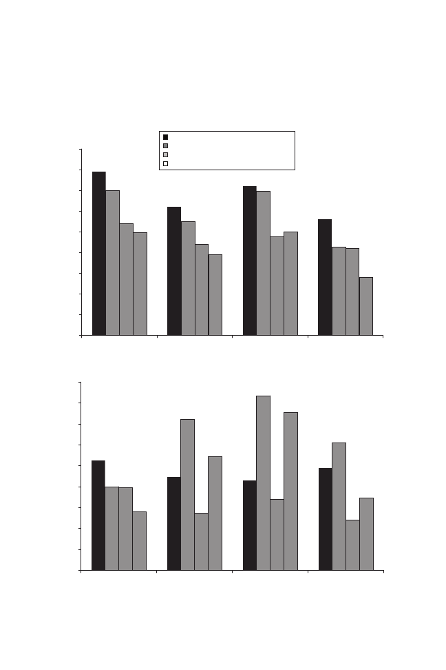
72 Hill, Holzer, and Chen

Figure 3.1 Effects of Household Structure on Outcomes, without and

with Controls for Parental Income

Without controls for parental income.

With controls for parental income.

Panel A: High school dropout/GED (percentage points)

Panel B: Unmarried with a child (percentage points)

0.0

2.0

4.0

6.0

8.0

10.0

12.0

14.0

16.0

18.0

Full sample

Blacks

Black males

Black females

0.0

2.0

4.0

6.0

8.0

10.0

12.0

14.0

16.0

18.0

Full sample

Blacks

Black males

Black females

***

15.8

***

14.0

***

10.8

***

9.9

***

12.4

***

11.0

8.8

7.8

***

14.4 ***

13.9

9.5

10.0

***

11.2

8.5

8.4

5.6

***

14.4

Mother never married

Mother had been married, no spouse in HH

Mother never married

Mother had been married, no spouse in HH

High school dropout/GED

Unmarried with a child

Ever incarcerated

***

13.9

9.5

10.0

8.6

***

16.7

6.8

***

15.1

***

14.9

7.8

***

13.4

6.5

***

10.5

***

8.0

***

7.9

***

5.6

8.9

***

14.4

5.5

***

10.9

8.6

***

16.7

***

15.1

6.8

9.8

12.2

4.8

6.9

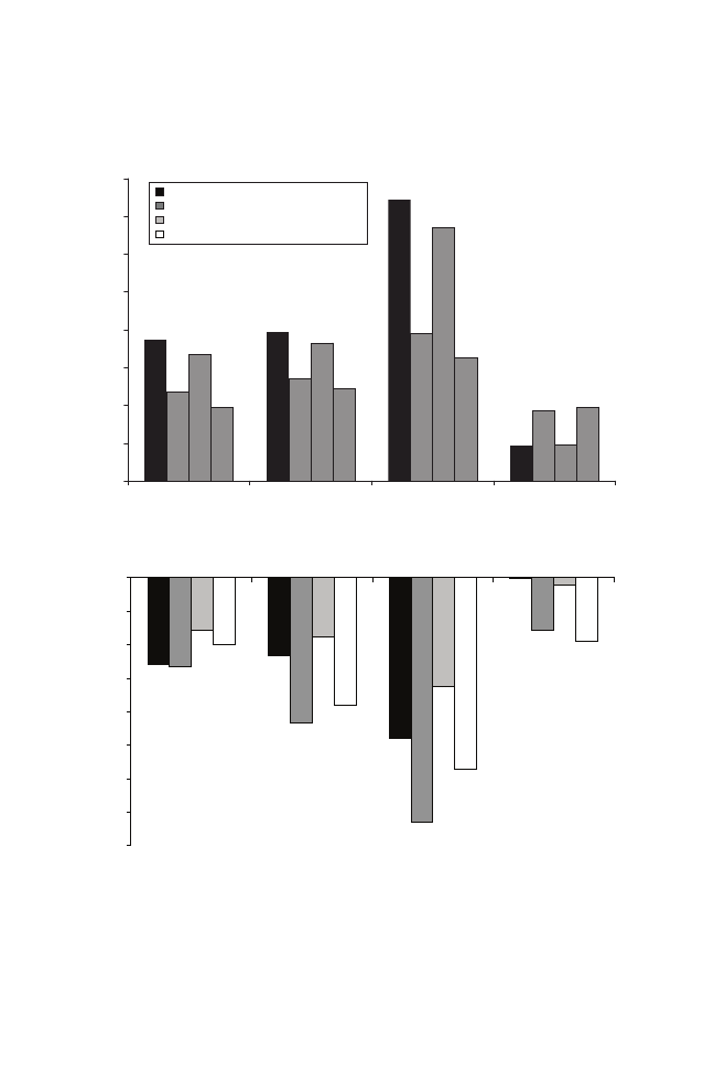
Household Structure and Young Adult Outcomes 73

Figure 3.1 (continued)

Panel C: Ever incarcerated (percentage points)

Panel D: Weeks worked (number of weeks)

0.0

2.0

4.0

6.0

8.0

10.0

12.0

14.0

16.0

Full sample

Blacks

Black males

Black females

***

7.5

***

4.7

***

6.7

***

3.9

***

7.9

***

5.4

***

7.3

***

4.9

***

14.9

7.8

***

13.4

6.5

1.9

3.7

1.9

3.9

***

14.4

Mother never married

Mother had been married, no spouse in HH

Mother never married

Mother had been married, no spouse in HH

High school dropout/GED

Unmarried with a child

Ever incarcerated

***

13.9

9.5

10.0

8.6

***

16.7

6.8

***

15.1

***

14.9

7.8

***

13.4

6.5

NOTE: Coefficients are from Table 3.4. Regression variables are measured in Round 8 of the NLSY97,

from October 2004 to July 2005. Average family income is measured for ages 14 to 15 for the
1982–1984 birth cohorts and 16 to 17 for the 1980–1981 birth cohorts. Control variables include

respondent’s age at Round 8 interview, mother’s age when she had her first child, whether mother is
an immigrant, number of siblings in the respondent’s household at age 16, mother’s educational at-
tainment, mother’s hours worked, month of Round 8 interview, and respondent’s household structure
at age 12. Missing data dummies were included for all explanatory variables except for race/gender.

Statistical significance is denoted as follows: * p < 0.10; ** p < 0.05; *** p < 0.01.

Without controls for parental income.

With controls for parental income.

−8.0

−7.0

−6.0

−5.0

−4.0

−3.0

−2.0

−1.0

0.0

Full sample

Blacks

Black males

Black females

−2.6

***

−2.7

***

−2.0

−1.6

−2.3

−1.8

−4.3

***

−3.8

−4.8

−7.3

***

−3.3

−5.7

−0.04

−1.6

−0.2

−1.9

74 Hill, Holzer, and Chen

cations (without and then with controls for parental income) separately
for each of four samples (the full sample, blacks, black males, and black
females). The same type of information is shown in the remaining pan-
els of Figure 3.1, with Panel B showing estimates from regressions pre-
dicting whether the sample member was unmarried with a child, Panel
C showing estimates from regressions predicting whether the sample
member was ever incarcerated, and Panel D showing estimates from
regressions predicting the number of weeks worked.

Observed differences in household structure, of course, may ac-

count for racial gaps in the employment, educational, and behavioral
outcomes examined here. We address this issue in Table 3.5 for each

of the seven outcomes. The first specification shows differences in out-
comes by race and gender with no control for household structure but
conditional on a number of sample member and maternal characteristics

(listed in the table’s endnote). Next, the second and third specifications
show differences by race and gender, adding in household structure co-

variates (specification 2) and then adding controls for family income

(specification 3). These latter two specifications correspond to those
shown in Table 3.4 for the full sample.

Consistent with the findings in Chapter 2, Table 3.5 shows strong

differences by race and gender in virtually every measured outcome,
even when controlling for a number of individual and maternal char-

acteristics in the first specification. Yet some outcome differences by
race and gender can be largely accounted for by differences in house-
hold structure. For instance, differences in the likelihood of enrolling
in and completing college between young white and black men largely
disappear when we control for household structure.

Differences in

dropping out of high school disappear once parental income is included
as a control. Because the ability of household structure and income to
account for racial differences in academic achievement (as measured
by the ASVAB) appears more limited, their estimated effects on differ-
ences in educational attainment likely work through other mechanisms
as well, such as youth attitudes or behaviors. The estimated effects of
household structure on incarceration were large (Table 3.4), and they
were consistent with the view that attitudinal and behavioral effects of
single parenthood on youth are substantial; indeed, in Table 3.5 half or
more of the racial differences among men are accounted for by includ-
ing controls for household structure and parental income.

Household Structure and Young Adult Outcomes 75

How much deterioration over time in employment, educational, and

risky behavioral outcomes for blacks is predicted by the changes in
family structure that have been observed since 1960—i.e., during the
overall period in which family structure changed quite dramatically in
the black community? We use estimates of these changes between 1960

and 1996, along with estimated coefficients from specification 1 for the
black subsample in Table 3.4, to predict such changes.

The results appear in Table 3.6. They suggest that the large changes

over time in the structure of black households have only modestly af-
fected labor market outcomes, reducing wages by about 2 percent and
weeks worked by about one week. But the predicted changes in educa-
tional attainment and performance are larger. The calculations suggest
that changes in household structure for blacks have added 4 percentage
points to their high school dropout rates and reduced college attendance
or completion by 5 percentage points, relative to means of 28 and 15
percent respectively for black males and 19 and 21 percent for black
females, (Table 2.2).

The changes’ effect on ASVAB percentile scores

(2.7 points) is relatively modest in comparison to means among young
blacks at roughly the thirtieth percentile (Table 2.3). They raise unmar-
ried childbearing by about 4 percentage points (a somewhat modest
increase in comparison to the black female mean of 48 percent or the
black male mean of 31 percent shown in Table 2.4), but by adding over
2 percentage points to the incarceration rate of black men (at 15 percent
in Table 2.5), they contribute a nontrivial amount to a costly phenom-
enon in the black community and in society.

Of course, there have been other, more positive developments in the

family backgrounds of blacks in this time period (such as rising parental
education and incomes) that have offset these predicted declines. But
the results of Table 3.6 suggest that, absent the changes that occurred
in black family structure between 1960 and 1996, the educational prog-

ress of the black community would have been significantly greater than
it has been, while the rise in incarceration and participation in other
risky behaviors among young blacks over time would not have been so
great.

Table 3.5 Effects of Race on Outcomes, without and with Controls for Household Structure and Parental Income

Natural log of hourly wage

Weeks worked

High school dropout/GED

(1)

(2)

(3)

(1)

(2)

(3)

(1)

(2)

(3)

Race/gender

Black male

−0.105

***

−0.093

***

−0.075

***

−7.538

***

−6.886

***

−6.207

***

0.074

***

0.035

0.002

(0.019)

(0.020)

(0.820)

(0.839)

(0.854)

(0.017)

(0.018)

Hispanic male

0.003

0.007

0.018

0.979

1.105

1.506

0.022

0.014

−0.007

(0.022)

(0.879)

(0.884)

(0.019)

White female

−0.162

***

−0.161

***

−0.162

***

−1.975

***

−1.936

***

−1.928

***

−0.024

−0.028

***

−0.029

***

(0.017)

(0.585)

(0.584)

(0.581)

(0.011)

Black female

−0.188

***

−0.175

***

−0.157

***

−7.184

***

−6.494

***

−5.773

***

−0.011

−0.052

***

−0.086

***

(0.019)

(0.020)

(0.774)

(0.803)

(0.817)

(0.015)

(0.016)

Hispanic female

−0.140

***

−0.135

***

−0.121

***

−4.525

***

−4.267

***

−3.807

***

−0.040

−0.053

***

−0.077

***

(0.022)

(0.897)

(0.900)

(0.908)

(0.019)

Household structure included

yes

Average family income included

yes

Observations

5,849

7,085

7,115

R-squared

0.087

0.088

0.093

0.056

0.059

0.065

0.119

0.138

0.154

Enrolled in four-year

college or not enrolled,

bachelor’s degree or more

ASVAB

Unmarried with a child

(1)

(2)

(3)

(1)

(2)

(3)

(1)

(2)

(3)

Race/gender

Black male

−0.062

***

−0.017

0.015

−22.709

***

−20.309

***

−17.751

***

0.143

***

0.116

***

0.099

***

(0.016)

(0.017)

(1.053)

(1.086)

(1.081)

(0.017)

Hispanic male

−0.066

***

−0.057

***

−0.035

−12.632

***

−12.031

***

−10.164

***

0.053

***

0.046

***

0.035

(0.018)

(1.307)

(1.302)

(1.275)

(0.017)

White female

0.078

***

0.083

***

0.084

***

2.047

2.249

***

2.229

***

0.076

***

0.073

***

0.073

***

(0.015)

(0.014)

(0.835)

(0.829)

(0.822)

(0.011)

Black female

0.005

0.052

***

0.083

***

−18.601

***

−16.092

***

−13.539

***

0.303

***

0.274

***

0.256

***

(0.017)

(1.045)

(1.081)

(1.076)

(0.017)

(0.018)

Hispanic female

−0.023

−0.011

0.015

−11.760

***

−10.934

***

−8.911

***

0.162

***

0.153

***

0.140

***

(0.019)

(1.321)

(1.310)

(1.296)

(0.020)

Household structure included

yes

Average family income included

yes

Observations

7,115

6,780

7,129

R-squared

0.177

0.199

0.219

0.316

0.328

0.346

0.126

0.134

0.138

(continued)

Ever incarcerated

(1)

(2)

(3)

Race/gender

Black male

0.045

***

0.028

0.023

(0.013)

Hispanic male

0.015

0.013

0.009

(0.013)

White female

−0.049

***

−0.050

***

−0.050

***

(0.007)

Black female

−0.058

***

−0.077

***

−0.083

***

(0.009)

(0.010)

Hispanic female

−0.067

***

−0.072

***

−0.076

***

(0.010)

(0.011)

Household structure included

yes

Average family income

included

yes

Observations

7,208

R-squared

0.277

0.286

0.287

NOTE: Robust standard errors clustered by family are shown in parentheses. Variables are measured in Round 8 of the NLSY97, from

October 2004 to July 2005. Average family income is measured from ages 14 to 15 for the 1982–1984 birth cohorts and from 16 to 17 for

the 1980–1981 birth cohorts. Control variables include respondent’s age at Round 8 interview, mother’s age when she had her first child,
whether mother is an immigrant, number of siblings in the respondent’s household at age 16, mother’s educational attainment, mother’s
hours worked, and month of Round 8 interview. Missing data dummies were included for all explanatory variables except for race/gender.

“White male” is the omitted race/gender category in the regressions. For a description of specifications (1), (2), and (3), see bottom of

p. 67/top of p. 68. Statistical significance is denoted as follows:

p < 0.10;

p < 0.05;

***

p < 0.01.

SOURCE: Authors’ tabulations from NLSY97.

Table 3.5 (continued)

Table 3.6 Predicted Changes in Outcomes for Blacks over Time (1960–1996) Due to Changes in Family Structure

Natural log of

hourly wage

Weeks

worked

High school

dropout/

GED

Enrolled in

4-year college

or not enrolled,

bachelor’s

degree or more

ASVAB

Unmarried

with a child

Ever

incarcerated

Person or persons with

whom sample member
lived at age 12

Mother, never married

−0.009

−0.452

0.024

−0.030

−1.592

0.017

0.015

Mother, had been

married, no spouse
in household

−0.005

−0.437

0.011

−0.012

−0.752

0.015

0.005

Mother and her spouse

−0.006

−0.232

0.004

−0.011

−0.369

0.007

0.004

Total

−0.020

−1.121

0.039

−0.053

−2.713

0.039

0.024

NOTE: Cell entries are equal to the product of the approximate percentage-point change over time in each household structure category

(see endnote in the text) multiplied by the coefficient on household structure from column (1) for the category “Blacks” in Table 3.4.

SOURCE: Authors’ tabulations from NLSY97.

80 Hill, Holzer, and Chen

Are the Estimated Effects of Household Structure Causal?

The estimated coefficients of Tables 3.4 and 3.5, and the predicted

outcomes for blacks over time that appear in Table 3.6, imply substan-
tial effects of household structure on a range of young adult outcomes.
But the possibility remains that instead of being causal, these effects
actually represent other unobserved characteristics of youth, their par-
ents, and their households that are correlated with both household struc-
ture and the outcomes. While we use a more extensive set of control
variables for other parental characteristics (including maternal weeks
worked) than other studies, the likelihood remains that some impor-
tant characteristics of parents or their children that are correlated with
household structure are still unobserved.

Our preferred method of dealing with this possible problem is to

estimate a series of fixed-effects models, based either on comparisons
between siblings or on comparisons over time for the same individual
(where multiple outcomes could be observed over time). The results of
all these tests appear in Table 3.7. Instead of showing each estimated

coefficient separately (the coefficients are mostly not statistically sig-

nificant in these models anyway), we present the p-values for F tests on

joint significance of the household structure variables. We also present

two versions of the individual fixed-effects model, using either a two-
year or a three-year lag between the points in time at which household
structure and outcomes are measured for any individual. We do not con-
trol for household income in these equations.

The results for the sibling fixed-effects models show only two

outcome equations in which the household structure variables remain

jointly significant: those for being enrolled in or having completed a
four-year college degree and those for ASVAB test score percentiles.

These findings are consistent with the findings of Sandefur and Wells
(1999), who found family structure effects on years of schooling using

sibling fixed-effects models with data from the NLSY79.

Our fixed-effect results are somewhat stronger for the individual

fixed effects: significant results (at least at the 0.10 level) appear for

five out of six outcomes that could be measured over time using a two-
year lag between observations of household structure and outcomes,

and for three out of six using a three-year lag. Using either lag, we find

significant effects of household structure on weeks worked and both

Table 3.7 Fixed-Effect Regressions with Controls for Mother’s Background and Household Structure at Age 12

Sibling regressions

Individual regressions

P-value for F-test

of whether age 12

household structure

dummies equal zero

Sample

size

P-value for F-test of

whether household

structure at interview

dummies (2-round

lag) equal zero

Sample

size

P-value for F-test of

whether household

structure at interview

dummies (3-round

lag) equal zero

Sample

size

Natural log of hourly wage

0.150

1,998

0.502

4,397

0.773

4,397

Weeks worked

0.312

2,862

0.000

***

6,658

0.000

***

6,658

High school dropout/GED

0.559

2,880

0.051

6,749

0.000

***

6,749

Enrolled in four-year

college or not enrolled,
bachelor’s degree
or more

0.021

2,880

0.000

***

6,749

0.000

***

6,749

ASVAB

0.000

***

3,010

Unmarried with a child

0.821

2,894

0.012

5,380

0.424

5,380

Ever incarcerated

0.836

2,960

0.018

6,627

0.217

6,627

NOTE: Robust standard errors are shown in parentheses. Variables are measured in Round 8 of the NLSY97, from October 2004 to July

2005. Control variables such as respondent’s race/gender, respondent’s age at Round 8 interview, mother’s age when she had her first
child, whether mother is an immigrant, number of siblings in the respondent’s household at age 16, mother’s educational attainment,
mother’s hours worked, and month of Round 8 interview were included but not reported in this table. Missing data dummies were includ-

ed for all explanatory variables except for race/gender. Statistical significance is denoted as follows:

p < 0.10;

p < 0.05;

***

p < 0.01.

SOURCE: Authors’ tabulations from NLSY97.

82 Hill, Holzer, and Chen

of our measures of educational attainment (i.e., dropping out of high
school and attending or completing a degree at a four-year college). The

shorter lag also generates significant effects of household structure on
being unmarried with a child or being incarcerated.

In our view, the limitations of fixed-effects models for estimating

these results likely lead to estimates that are biased toward a finding of

no significant effect at all. In particular, the limitations are that a rela-
tively small number of individuals or sibling pairs actually experience
changes in household structure in the relevant time period (especially
for the never-married mothers), and the time period during which any
such changes can generate observable changes in behavior or outcomes
is limited. Given that only two years in age separate the average pair

of siblings in our data, it is perhaps not surprising that few significant
results were observed for them; in contrast, the time periods over which
differences are observed in the individual models are longer, at four

years. But the fact that most of the individual fixed-effects in the two-

year lag (and some in the other models) are significant suggests that at
least some part of the estimated effects of household structure on youth
outcomes is causal. Based on these estimates, however, it is very dif-

ficult to say exactly how much.

Our inability to pin down causal magnitudes more precisely here is

a limitation of this work. Perhaps other estimation strategies, such as
instrumental variables, might be more successful (though we note our
own reservations about the use of these strategies to date in Chapter 1).
Nevertheless, showing that at least some parts of our estimated effects
are causal implies that the issue of household structure is a serious one,
and thus it is important to understand more about exactly what are the
mediating variables and mechanisms through which it works, as well as
its potentially offsetting effects.

CONCLUSION

In this chapter, we present data on differences in household struc-

ture at age 12 for white, black, and Hispanic youth in the NLSY97. We
also estimate the effects of household structure on a set of seven em-
ployment, educational, and behavioral outcomes and show differences

Household Structure and Young Adult Outcomes 83

by race. Finally, we estimate sibling and individual fixed-effects models
to explore the extent to which the estimated effects are causal.

Our results suggest the following:

• Roughly one-half of all youth, and about four-fifths of black

youth, do not live with both of their biological parents at age 12.

• Youth living without both biological parents, and especially with

never-married mothers, are in households with substantially
lower incomes when growing up, though this at least partly re-

flects other differences in parental characteristics (such as lower
maternal education).

• Growing up without both biological parents is associated with

modest reductions in wages and weeks worked for young adults,
and more substantial reductions in educational attainment or
achievement for them, as well as greater participation in risky or
illegal behaviors.

• Lower family income accounts for less than half of these esti-

mated effects in most cases.

• The greater tendency of young blacks to grow up in families

without both biological parents, and especially with never-
married mothers, accounts for fairly large parts of the racial dif-
ferences in educational attainment and some risky behaviors
among young men, and also for some of the limited progress (or
actual deterioration) over time for blacks in these outcomes.

• Fixed-effects regression models for these outcomes—either

across sibling pairs or over time for individuals—suggest that at
least some part of the estimated relationships between household
structure and these outcomes is causal, though we cannot infer
the exact magnitudes.

Overall, the fact that large fractions of youth—especially black

youth—grow up without both biological parents has negative implica-
tions for a range of outcomes during their teen and young adult years,
especially those involving education and risky behaviors. Recent trends
in household structure would appear to be at least partly responsible for
the persisting black-white gaps in educational attainment and achieve-
ment, as well as the cycle of unmarried childbearing and dramatic in-
creases in crime and incarceration that have affected black youth in

84 Hill, Holzer, and Chen

general and young black men in particular. These findings are consistent
with those of Sara McLanahan, Gary Sandefur, Daniel Lichter, Frank
Furstenberg, and others noted in Chapter 1.

Some words of caution, however, are in order. For one, our analysis

in this chapter does not explore the causes of household structure and its
trends among blacks and other racial groups. A large literature does this
elsewhere (see Chapter 1) and suggests that the causes of these trends
lie partly in labor market changes (such as declining wages of less-
educated men and rising relative wages of women) as well as in other

demographic and attitudinal changes. Drawing firm conclusions about
the possibly negative effects of these trends without understanding their
causes might lead one to prematurely advocate for certain changes in
behavior or policy that might not address the true causes.

Furthermore, it is likely—at least from the correlations we observe

between household structure and maternal education—that some parts
of the simple statistical relationships observed between household
structures and outcomes are not causal. While we can easily control for
maternal educational differences across individuals in our regression
equations, we likely cannot observe or control for all of the relevant dif-
ferences between youth or their parents that might affect these outcomes
(such as the poorer families in which many single mothers themselves

grew up). And while the various fixed-effects models we estimate seem
to offer our best chance to account for these kinds of differences within
these data, their limitations have also been clearly noted above.

It is also important to note that, despite the important effects of

household structure on outcomes that we estimate, large racial gaps in
most of these outcomes remain even after controlling for racial differ-
ences in household structure. This is particularly true for the large racial
gaps in employment outcomes between young white and black men, but
is also true for various gaps in educational achievement, unmarried par-
enthood, and incarceration. To note those parts of the gaps in outcomes
for which we can account without acknowledging the parts for which
we cannot account would be misleading.

Having stated these caveats, the task remains of gaining a better un-

derstanding of the mechanisms through which single parenthood nega-
tively affects outcomes for youth and young adults, especially among
blacks. If the disadvantages associated with growing up in single-parent

families mostly do not stem from their lower incomes, as our findings

Household Structure and Young Adult Outcomes 85

seem to show, what other factors are at play? To what extent do these
disadvantages grow out of parental attitudes and behaviors that might
themselves be at least partial products of single parenthood? Are the
true negative effects reinforced by other disadvantages—disadvantages
associated with characteristics unique to the families or parents them-
selves or to the neighborhoods in which they live? At the same time,
can these negative effects be offset by other choices and activities of
parents, as Furstenberg et al. (1999) imply?

We turn to these questions in the next chapter.

Notes

1. For example, using additional information from the household rosters, we estimate

that cohabiters make up just one-half of 1 percent of biological parent households
and 5 percent of unmarried mother households (a combined category of never-
married and previously married).

2. When only one year of income information was available, information from that

year was used instead of setting the variable to missing.

3. We examined the correlations of single-year, two-year-average, and three-year-

average income across different ages for available subsamples of youth. Single-
year correlations ranged from 0.6 to 0.7, with higher correlations in concurrent
years, as expected. Also as expected, correlations between two-year averages were
higher (0.7 to 0.9), and correlations among three-year averages were highest (0.8
to 0.9).

4. Ideally, we would measure number of siblings in the sample member’s household

at the same time that household structure is measured (i.e., at age 12) or as close as
possible to that age. Because of the age ranges of the youth initially surveyed, the
age closest to age 12 at which we can measure number of siblings (including step
and adoptive siblings) in the household, using the household rosters, is age 16.

5. The year 1996 corresponds to the time when sample members turned 12 to 16

years old. Whether maternal employment should be controlled for in all of these
equations is debatable, if this measure is itself heavily affected by single-parent
status. Our estimated outcome equations that do not include this control variable
are qualitatively similar, but they do show somewhat greater effects of household
income on the estimated household structure effects. These estimates are available
from the authors upon request.

6. We also ran the models using household structure at age 6, but the results were not

sensitive to this difference in timing.

7. Because it does not change over time, the outcome ASVAB is not estimated using

individual fixed effects.

8. Our reduced-form OLS equations did not specify a particular time period during

which household structure at age 12 should affect education, employment, and

86 Hill, Holzer, and Chen

behavioral outcomes among youth and young adults. But with individual fixed-
effects models, these timing choices must be made more explicitly, because the
exact timing of changes in household structure will now drive the changes in out-
comes we seek to measure.

9. Of course, if the families that change household structure are not random, it is at

least possible for the bias to go in the opposite direction.

10. Sample weights are used in the summary statistics, but not in the regression

analyses.

11. Data from the NLSY79 and NLSY97 capture changes in household structure that

occurred only during the 1980s and early 1990s. Additional tabulations show that

the percentage of young blacks aged 14 to 18 at the time of the first survey round
(1979 and 1997, respectively) who did not live with both biological parents rose
from 59 percent to 73 percent between the two cohorts.

12. Among youth living with never-married mothers, 28.8 percent of black youth

have mothers who were high school dropouts, compared with 38.5 percent of
white youth and 46.1 percent of Hispanic youth.

13. The estimated influence of parental income was somewhat sensitive to the specific

time period used. Part of the difficulty is that a consistent two-year (or greater)
average family income cannot be calculated for all sample members across com-

parable years. Another part of the difficulty has to do with measurement error in
the variable. Of all the parental income measures we examined for the full sample,
the one we use in the estimated models has the greatest impact on reducing the
effects of household structure.

14. In a few cases, the estimated effects for blacks are larger; these include the ef-

fects of having a never-married or a divorced-but-not-remarried mother on wages,
and the effects of having a mother previously married but without a spouse on
weeks worked and on the probability of having a child outside of marriage. In a
variety of other cases, the estimated differences are a bit larger for the sample that
includes whites and Hispanics. Most of these differences in estimated effects are

only marginally significant at best, even though the Chow tests indicate statisti-

cally significant differences between equations estimated overall for blacks versus
nonblacks.

15. Differences in educational attainment between white and black females can be

inferred from comparisons between their coefficients (each measured relative to

white males) and how the differences change across specifications. The racial dif-
ference in dropout behavior among young women is smaller than among young
men, without and with the household controls, though the differences in college
attendance or completion between young white and young black women are also

narrowed significantly by these controls.

16. Our data on black family structure in 1960 are from Ellwood and Crane (1990).

The family structure categories they use for describing the living arrangements of
black children are “married couple,” “divorced, separated, or widowed parent,”
“never-married parent,” and “not with a parent.” Comparing their numbers for
1960 (in Table 1) with ours for 1996 (Table 3.1, above), and making some as-
sumptions about the gender distribution of their single-parent categories, we infer

Household Structure and Young Adult Outcomes 87

that the fraction of black children living with both biological parents declined by
roughly 40 percentage points (from about 0.60 to 0.20) and rose in the “never
married,” “divorced,” and “remarried” mother categories by about 0.18, 0.10, and
0.12, respectively. The results in Table 3.7 are not very sensitive to small changes
in the distribution of the 40-percentage-point decline.

17. The means for the latter category were obtained by summing the portions in the

Table 2.2 categories for “not enrolled, bachelor’s degree” and “enrolled, four-year
college.”

Other Correlates of

Household Structure and

Their Effects on Outcomes

The previous chapter showed strong statistical relationships be-

tween household structure and a range of employment, educational, and
behavioral outcomes of young adults—both for the full sample and for
the subgroup of blacks. While family income accounted for a consider-
able portion (up to 40 percent) of the effects of household structure on

outcomes, significant portions remained, both statistically and substan-

tively. Results from fixed-effects models suggested some causal role for
household structure on outcomes, as well.

But how and why do household structures affect these outcomes?

What are the mechanisms that account for the weaker performance of
youth who have lived in single-parent households? Are these mecha-

nisms themselves causal, and do they reflect causal effects of household
structure? Or are they just spuriously related to household structure and
to the outcomes themselves?

In this chapter, we further explore three types of household charac-

teristics that are likely to be correlated both with household structure
and with the employment, educational, and behavioral outcomes we
examine. They are measures of 1) human capital enrichment, 2) parent-
ing and home environment, and 3) neighborhood characteristics.

Using information from a subset of the NLSY97, we first show how

measures in each of the three categories are associated with household
structure. Next, we present regression models similar to those shown in
Chapter 3, but now with these three types of household characteristics
having been added. We show how the estimated effects of household
structure differ once these characteristics are included in the models.

We also show the joint influence of each of these three categories of
variables on the outcomes.

The evidence presented in this chapter indicates that the three sets

of household characteristics we examine do account for some of the

90 Hill, Holzer, and Chen

statistical associations between household structure and outcomes.
Furthermore, these characteristics themselves are associated statisti-
cally, and in some cases substantively, with the outcomes we examine.
Thus, they help us better understand why the household structures in
which young people grow up might affect their later outcomes in life,
and they suggest how these effects might be addressed through policy
interventions.

SAMPLE AND MEASURES

The analysis in this chapter uses a subsample of NLSY97 respon-

dents born from 1982 to 1984, who were mostly ages 20 to 22 at the
time of the Round 8 interview in 2004–2005. This sample restriction
is necessary because some of the additional measures we analyze were
collected (by survey design) only for these younger members of the
cohort.

The NLSY97 collects a rich set of information about sample mem-

bers’ home and neighborhood environments and relationships with
parents and peers.

We select a relatively small subset of 11 of these

variables for further investigation in this chapter. These reflect the three
overarching constructs of 1) human capital enrichment, 2) parenting
and home environment, and 3) neighborhood characteristics.

We examine the extent to which the 11 variables reduce the esti-

mated associations between household structure and the various out-
comes, as well as the extent to which they themselves provide explana-
tory power for these outcomes.

There are good theoretical reasons for believing that these three sets

of factors at least partly account for the observed effects of household
structure on youth outcomes, as we note below. But, within each con-
struct, we also had to choose from among a wide variety of variables
in the NLSY that were conceptually similar and often fairly highly cor-
related with one another. As described further below, we selected 11
variables in all that had face validity for representing each construct,
were not too strongly correlated with each other, and were related to the
outcomes we examined (individually and as a group).

Other Correlates of Household Structure and Their Effects 91

Our intent was not, as has been successfully done elsewhere (Child

Trends 1999), to develop or use a composite index for different con-
structs, but instead to select a few representative measures in each area
that would be reasonable and readily interpretable. We acknowledge the
limitations of some of these measures and encourage future research

that would refine the measures and further investigate their relation-
ships with household structure and the range of outcomes presented

here. Our work should thus be viewed as exploratory, rather than defini-
tive, in some ways.

Why should these three sets of measures be related both to house-

hold structure and to youth outcomes? Regarding human capital, it ap-
pears that access to enriching and material resources early in life may

promote positive youth development and directly or indirectly influence
outcomes in early adulthood (e.g., Beltran, Das, and Fairlie 2006). To

reflect such human capital enrichment, we use three self-reported mea-
sures (variables 1 through 3) from the 1997 Round 1 of the NLSY97
(when respondents were generally 12 to 14 years old):

1) whether there was usually a computer in the home in the previ-

ous month,

2) whether there was a dictionary in the home in the previous

month, and

3) whether the youth spent any time taking extra classes or

lessons.

Regarding parenting and the home environment, the literature points

to the importance of parents’ support of, connection to, and regulation
of their children (Barber and Olsen 1997; Dornbusch et al. 1987; Eccles
et al. 1997; Slicker 1998; Steinberg et al. 1992; Tepper 2001). Regula-
tion includes monitoring or setting limits, as well as offering or impos-
ing structure through activities such as enrolling the children in extra-
curricular classes or doing things together as a family. Furthermore,

the physical home environment—specifically, the orderliness of the
home—is related to educational and labor market outcomes, suggesting

that parents can influence noncognitive factors as well (Dunifon, Dun-
can, and Brooks-Gunn 2001). With variables 4 though 9, we examine
six measures of parenting and home environment, all self-reported by
the youth in Round 1 except where noted below. We measure:

92 Hill, Holzer, and Chen

4) how supportive the youth perceived his or her mother or

mother figure to be (originally measured on a three-point scale,
which we standardized to have a mean of zero and variance of
one so that a one-unit increase in the variable corresponds with
a one-standard-deviation increase);

5) whether the youth perceived his or her mother to be strict

(compared to being permissive);

6) how much the youth thought his or her mother knew about

whom the youth was with when the youth was not at home

(measured on a five-point Likert scale, which we standardized
to have a mean of 0 and a variance of 1);

7) how well-kept the interior of the youth’s home was (as as-

sessed by the interviewer on a three-point Likert scale, which
we standardized to have a mean of 0 and variance of 1);

8) the number of days in a typical week that housework got done

when it was supposed to; and

9) the number of days during a typical week that the family ate

dinner together (a measure of structure).

Finally, the quality of the physical and social neighborhood in

which children and youth grow up may also affect their development
and their future opportunities (Sampson, Raudenbush, and Earls 1997;
Wilson 1987). With variables 10 and 11, we examine two measures of
neighborhood quality from Round 1 of the NLSY:

10) the number of days a week that gunshots are not usually heard

(self-reported by the sample member);

and

11) a measure of how well kept buildings were in the neighbor-

hood where the youth lived (a subjective rating on a three-
point Likert scale by the interviewer, standardized to have a
mean of 0 and variance of 1).

For each of these three overarching constructs, there is reason to

believe that these measures will be correlated with household structure
as well as youth outcomes. For instance, single parents who themselves
are less educated and have weaker cognitive achievement might expose
their children to less human capital enrichment; their lower incomes
and other social ties might cause them to live in poorer neighborhoods;

Other Correlates of Household Structure and Their Effects 93

and they might be less able to supervise their children and maintain
orderly households, given the pressures of work and the instability of
their lives. Clearly, some of these correlations with household structure
might be spurious (especially those relating to human capital enrich-

ment), some might reflect the lower incomes of these households (like
enrichment and neighborhood quality), and others might be truly causal

(especially those reflecting parenting and the home environment). With
these expectations, we turn to the estimation and empirical results.

ESTIMATED EQUATIONS

Following McLanahan and Sandefur (1994), Furstenberg et al.

(1999), and others, we build on the model specifications of Chapter 3
to now add the human capital, parenting and home environment, and
neighborhood variables just described:

(4.1) Y

= f (HH

, X

, M

, I

, W

)

+ ε

where Y, HH, X, M, and I

are all defined as they were in Chapter 3. W

represents the set of household characteristics related to human capital
enrichment, parenting and home environment, and neighborhood char-
acteristics. We control for family income and other characteristics in
Equation (4.1). Even so, the observed relationships between household
structure and these household characteristics may be spurious.

We acknowledge, of course, that the estimated effects of these three

sets of additional explanatory variables—like those of household struc-
ture—are not necessarily causal. Instead, we aim to produce a set of
conditional estimates of household structure and household character-
istics, related to a range of young adult outcomes. These estimates il-
lustrate the potential mediating effects of these characteristics, and they
also provide a sense of any remaining effects of household structure on
these outcomes. But in the next section we also consider some reasons

why these estimated effects might in part reflect causal relationships.

94 Hill, Holzer, and Chen

EMPIRICAL RESULTS

This section first presents descriptive statistics on the 11 household

characteristics just described, separately by household structure for
the full sample as well as for the subgroup of black sample members.
Next, results from regression analyses that include these measures are
presented.

Descriptive Statistics

Sample means for each of the 11 variables are shown in Table 4.1,

separately by household structure, both for the full sample and for the
black subgroup.

Each of the measures of human capital enrichment, parenting, and

neighborhood characteristics shows clear associations with household
structure. For example, over 70 percent of all youth with both biologi-
cal parents present report having a computer in the home, while only
about 21 percent of youth in households with never-married mothers
do so. Forty-two to 57 percent of youth living in other types of house-
holds generally report the presence of computers. Similar patterns are
observed for other enrichment measures, though with somewhat less
variation across the household categories. For instance, over 90 percent
of youth in each household type report having a dictionary, but the per-
centages range from 91 percent among households run by never-married
mothers to 98 percent among those with two biological parents present.
Similarly, the percentages of youth who report taking extra classes or
lessons range from about 18 percent in households headed by fathers
(with the biological mother not present) to 34 percent in households
with two biological parents.

With regard to the neighborhood quality measures, the average

youth in a household headed by a never-married mother reports not
hearing gunshots about 6 days a week, whereas those living with two
biological parents do not hear them about 6.7 days a week; also, inter-
viewers report less well-kept buildings where the former live, relative
to the latter.

Parenting measures tell a similar, though somewhat more mixed,

story. For the full sample, youth in households with two biological par-

Other Correlates of Household Structure and Their Effects 95

ents report having supportive mothers (relative to the mean) while those
with never-married mothers report the opposite. The mothers perceived
as being least supportive are those of youth living with their fathers or
others, which is consistent with what one might expect. The association
between perceived maternal strictness and household structure is weak-
er, as never-married mothers are considered the most strict but those
previously married (with no spouse currently present) the least strict.
These associations correspond to previous research showing that strict-
ness is often used by single parents to manage youth in harsh neighbor-
hood environments (e.g., Furstenberg et al. 1999).

For the full sample, maternal knowledge of youth companions is

greatest in two-parent families and lowest among never-married mothers
and others (except for those youth living with their fathers). Homes ap-
pear best-kept in two-parent families and least-well-kept among never-
married mothers, and a similar pattern is observed for the regularity
with which meals are eaten together. But the ability of parents to get
housework done follows a more mixed pattern.

As for racial differences in these measures, young blacks report

fewer computers, less safe neighborhoods, and stricter parenting within
each household category, compared to the full sample. Within the black
subgroup, for the most part the patterns of association between each
measure and household structure are similar to those of the full sample:
black youth living with two biological parents are the most likely to
have computers and dictionaries, are least likely to hear gunshots, most
likely to live where there are well-kept buildings on the street, and most
likely to have mothers who are knowledgeable about their companions.
For some measures, however, such as taking extra lessons or maternal
strictness, strong associations are not apparent.

Overall, the results of Table 4.1 show strong associations between

household structure and the human capital enrichments to which young
people have access, the home environment and parenting they experi-
ence, and the neighborhood environments in which they grow up.

Regression Estimates for Seven Key Outcomes

Table 4.2 shows coefficient estimates on household structure indi-

cators for each of seven outcomes, with two specifications per outcome:
Equation (3.2), which controls for maternal characteristics and family

Table 4.1 Means on Household and Parenting Characteristics by Household Structure at Age 12

Enrichment

Neighborhood

In the past month,

has your home

usually had a

computer? (%)

In the past month,

has your home

usually had a

dictionary? (%)

In a typical

week, did you

spend any time

taking extra classes

or lessons? (%)

In a typical week,

how many days
do you not hear

gunshots in your

neighborhood?

How well-kept

are the buildings

on the street where

the youth lives?

(mean = 0, var. = 1)

Full

sample

Blacks

Full

sample

Blacks

Full

sample

Blacks

Full

sample

Blacks

Full

sample

Blacks

Total

58.0

35.9

95.8

92.9

28.5

29.3

6.55

6.17

0.11

−0.36

At age 12, sample member
lived with:

Both biological parents

72.1

53.4

98.0

99.3

33.7

28.6

6.65

6.39

0.34

−0.07

Mother, never married

20.9

20.1

91.1

92.9

22.7

28.7

6.05

5.74

−0.51

−0.71

Mother, had been married,

no spouse in household

46.0

34.6

94.3

91.4

26.8

28.3

6.59

6.07

−0.13

−0.32

Mother and her spouse

49.6

37.4

93.5

90.1

25.3

29.6

6.48

6.28

−0.01

−0.26

Father

57.4

43.4

95.1

94.8

17.9

27.7

6.43

6.37

−0.09

−0.37

Other

42.1

31.5

93.5

92.3

25.0

34.8

6.41

6.27

−0.07

−0.49

Sample size

4,412

1,185

4,410

1,185

4,392

1,181

4,384

1,166

3,910

1,052

Parenting

Mother is

supportive

(mean = 0,

var. = 1)

Mother is strict

Mother’s

knowledge of

respondent’s

companions

when she is not

home (mean = 0,

var. = 1)

How well-kept is

the interior of the

youth’s home?

(mean = 0,

var. = 1)

Number of

days per week

housework gets

done when it is

supposed to?

Number of

days per week

respondent
eats dinner

with family?

Full

sample Blacks

Full

sample Blacks

Full

sample Blacks

Full

sample Blacks

Full

sample Blacks

Full

sample Blacks

Total

−0.05 −0.13

56.0

63.2

0.01

−0.08

0.05

−0.19

5.63

5.53

5.17

4.53

At age 12, sample member
lived with:

Both biological parents

0.10

−0.06

57.1

63.1

0.12

0.04

0.24

0.08

5.70

5.53

5.33

4.50

Mother, never married

−0.17 −0.19

62.3

65.3

−0.13 −0.16 −0.37 −0.52

5.54

5.64

4.58

4.43

Mother, had been married,

no spouse in household

−0.16 −0.11

50.1

63.7

−0.04

0.02

−0.16 −0.14

5.33

5.11

4.86

4.59

Mother and her spouse

−0.13

0.00

54.4

60.6

−0.02 −0.08 −0.05 −0.11

5.71

5.82

5.20

4.56

Father

−0.36

−0.47

61.8

62.0

−0.42

−0.40

−0.31 −0.25

5.58

5.66

5.21

4.39

Other

−0.33

−0.42

53.4

61.9

−0.13

−0.28

−0.03 −0.41

5.70

5.49

5.33

4.84

Sample size

4,259

1,140

4,250

1,138

4.257

1,140

3,811

1,026

4,373

1,163

4,376

1,164

NOTE: Table includes respondents born between 1982 and 1984.

Household structure is measured at age 12, but these youth were asked about these topics in Round 1, when some of them were older.

Therefore, some youth were living with their mothers or with mother figures by this time.

SOURCE: Authors’ tabulations from NLSY97.

Table 4.2 Effects of Household Structure on Outcomes: without and with Neighborhood and Parenting

Characteristics

Natural log of hourly wage

Full sample

Blacks

Black males

Black females

(1)

(2)

(1)

(2)

(1)

(2)

(1)

(2)

At age 12, sample member lived with:

Mother, never married

0.000

0.002

−0.035

−0.042

−0.099

−0.117

0.021

0.027

(0.028)

(0.044)

(0.047)

(0.056)

(0.055)

(0.071)

(0.076)

Mother, had been married, no spouse

in household

0.006

0.008

−0.016

−0.056

−0.048

0.017

0.026

(0.026)

(0.050)

(0.068)

(0.065)

(0.077)

(0.079)

Mother and her spouse

0.036

0.035

−0.055

−0.054

−0.050

−0.040

−0.056

−0.050

(0.022)

(0.043)

(0.044)

(0.053)

(0.052)

(0.067)

(0.068)

Father

0.017

0.043

−0.017

0.004

−0.138

−0.100

0.129

0.116

(0.050)

(0.055)

(0.077)

(0.088)

(0.081)

(0.083)

(0.141)

(0.179)

Other

0.028

0.026

0.045

0.038

−0.018

−0.047

0.101

0.090

(0.035)

(0.056)

(0.058)

(0.060)

(0.057)

(0.093)

(0.101)

Enrichment, neighborhood, and

parenting variables included

yes

Observations

3,604

904

429

475

R-squared

0.065

0.071

0.073

0.092

0.084

0.159

0.095

0.107

Weeks worked

Full sample

Blacks

Black males

Black females

(1)

(2)

(1)

(2)

(1)

(2)

(1)

(2)

At age 12, sample member lived with:

Mother, never married

−1.259

−0.752

−2.454

−1.380

−5.851

−3.685

−0.015

0.574

(1.308)

(2.119)

(2.141)

(2.980)

(2.982)

(3.041)

(3.066)

Mother, had been married, no spouse

in household

−0.806

−0.408

−3.749

−2.865

−5.476

−3.820

−2.172

−1.857

(1.007)

(1.009)

(2.268)

(2.297)

(3.191)

(3.212)

(3.258)

(3.325)

Mother and her spouse

0.459

0.757

−0.755

0.139

−2.028

−0.614

0.060

1.233

(0.878)

(0.885)

(2.059)

(2.058)

(2.966)

(3.015)

(2.820)

(2.869)

Father

−0.482

0.366

4.018

4.519

6.110

9.160

0.102

−2.067

(1.886)

(2.061)

(3.824)

(4.264)

(4.857)

(5.403)

(5.829)

(6.441)

Other

−3.561

−3.436

−2.009

−1.171

−4.378

−2.557

0.467

1.718

(1.468)

(1.483)

(2.542)

(2.609)

(3.838)

(3.996)

(3.431)

(3.533)

Enrichment, neighborhood, and

parenting variables included

yes

Observations

4,364

1,166

557

609

R-squared

0.065

0.075

0.073

0.102

0.105

0.156

0.091

0.142

(continued)

100

Table 4.2 (continued)

High school dropout/GED

Full sample

Blacks

Black males

Black females

(1)

(2)

(1)

(2)

(1)

(2)

(1)

(2)

At age 12, sample member lived with:

Mother, never married

0.120

***

0.086

***

0.094

0.065

0.109

0.055

0.088

0.075

(0.029)

(0.043)

(0.042)

(0.064)

(0.067)

(0.058)

(0.057)

Mother, had been married, no spouse

in household

0.090

***

0.070

***

0.096

0.083

0.138

0.114

0.043

0.047

(0.020)

(0.041)

(0.060)

(0.063)

(0.054)

Mother and her spouse

0.076

***

0.058

***

0.001

−0.011

−0.029

−0.069

0.021

0.018

(0.018)

(0.017)

(0.035)

(0.034)

(0.053)

(0.054)

(0.045)

(0.046)

Father

0.087

0.064

0.010

0.028

0.138

0.091

−0.148

−0.065

(0.039)

(0.042)

(0.068)

(0.073)

(0.100)

(0.109)

(0.084)

(0.088)

Other

0.084

***

0.071

0.051

0.044

0.066

0.041

0.035

0.023

(0.031)

(0.030)

(0.053)

(0.052)

(0.081)

(0.082)

(0.067)

(0.064)

Enrichment, neighborhood, and

parenting variables included

yes

Observations

4,396

1,186

568

618

R-squared

0.153

0.185

0.173

0.213

0.190

0.240

0.193

0.248

101

Enrolled in 4-year college or not enrolled, bachelor’s degree or more

Full sample

Blacks

Black males

Black females

(1)

(2)

(1)

(2)

(1)

(2)

(1)

(2)

At age 12, sample member lived with:

Mother, never married

−0.128

***

−0.089

***

−0.094

−0.067

−0.098

−0.063

−0.098

−0.092

(0.022)

(0.040)

(0.046)

(0.049)

(0.063)

Mother, had been married, no spouse

in household

−0.092

***

−0.065

***

−0.041

−0.014

−0.073

−0.029

−0.010

−0.006

(0.021)

(0.020)

(0.044)

(0.053)

(0.055)

(0.071)

Mother and her spouse

−0.131

***

−0.110

***

−0.078

−0.067

−0.018

−0.128

−0.119

(0.019)

(0.042)

(0.058)

(0.057)

(0.062)

(0.061)

Father

−0.150

***

−0.101

***

−0.075

−0.058

−0.038

−0.003

−0.178

−0.156

(0.033)

(0.036)

(0.069)

(0.075)

(0.092)

(0.098)

(0.105)

(0.115)

Other

−0.106

***

−0.085

***

−0.062

−0.052

−0.069

−0.061

−0.063

−0.045

(0.027)

(0.048)

(0.055)

(0.058)

(0.075)

Enrichment, neighborhood, and

parenting variables included

yes

Observations

4,396

1,186

568

618

R-squared

0.229

0.263

0.162

0.197

0.137

0.192

0.221

0.263

(continued)

102

Table 4.2 (continued)

ASVAB

Full sample

Blacks

Black males

Black females

(1)

(2)

(1)

(2)

(1)

(2)

(1)

(2)

At age 12, sample member lived with:

Mother, never married

−5.101

***

−2.736

−1.276

0.426

−1.099

1.191

−0.730

0.481

(1.538)

(1.513)

(2.240)

(2.219)

(3.044)

(3.167)

(3.263)

(3.209)

Mother, had been married, no spouse

in household

−2.901

−1.311

−2.160

−0.473

−2.711

−0.355

−1.480

−1.156

(1.278)

(1.250)

(2.364)

(2.328)

(3.225)

(3.257)

(3.530)

(3.528)

Mother and her spouse

−3.363

***

−2.000

2.058

3.221

4.360

5.166

−0.032

1.656

(1.218)

(1.183)

(2.274)

(2.256)

(3.233)

(3.330)

(3.005)

(3.064)

Father

−4.222

−3.743

1.507

1.859

2.946

3.052

−0.549

1.090

(2.274)

(2.319)

(3.334)

(3.401)

(4.727)

(4.694)

(5.161)

(5.339)

Other

−5.587

***

−4.925

***

−0.343

0.479

0.760

1.443

−1.716

−0.622

(1.826)

(1.856)

(2.664)

(2.667)

(3.682)

(3.849)

(3.863)

(3.675)

Enrichment, neighborhood, and

parenting variables included

yes

Observations

4,103

1,072

543

529

R-squared

0.349

0.387

0.267

0.304

0.241

0.286

0.310

0.357

103

Unmarried with a child

Full sample

Blacks

Black males

Black females

(1)

(2)

(1)

(2)

(1)

(2)

(1)

(2)

At age 12, sample member lived with:

Mother, never married

0.125

***

0.098

***

0.054

0.020

0.119

0.099

0.005

−0.003

(0.029)

(0.030)

(0.044)

(0.045)

(0.064)

(0.067)

(0.066)

(0.067)

Mother, had been married, no spouse

in household

0.050

***

0.036

0.048

0.022

0.131

0.098

−0.041

−0.039

(0.019)

(0.044)

(0.063)

(0.065)

Mother and her spouse

0.065

***

0.052

***

0.046

0.021

0.050

0.049

0.045

0.021

(0.017)

(0.043)

(0.058)

(0.061)

(0.063)

(0.064)

Father

0.080

0.060

0.038

0.025

0.022

0.004

0.134

0.152

(0.038)

(0.039)

(0.076)

(0.081)

(0.112)

(0.123)

(0.106)

(0.108)

Other

0.085

***

0.076

0.063

0.047

0.154

0.160

0.001

−0.012

(0.029)

(0.030)

(0.052)

(0.054)

(0.084)

(0.086)

(0.072)

(0.073)

Enrichment, neighborhood, and

parenting variables included

yes

Observations

4,401

1,184

566

618

R-squared

0.136

0.154

0.107

0.130

0.096

0.132

0.144

0.176

(continued)

104

Table 4.2 (continued)

Ever incarcerated

Full sample

Blacks

Black males

Black females

(1)

(2)

(1)

(2)

(1)

(2)

(1)

(2)

At age 12, sample member lived with:

Mother, never married

0.079

***

0.066

***

0.084

***

0.071

***

0.163

***

0.140

***

0.014

0.016

(0.018)

(0.024)

(0.044)

(0.021)

Mother, had been married, no spouse

in household

0.043

***

0.036

***

0.052

0.051

0.058

0.042

0.054

0.067

(0.012)

(0.023)

(0.036)

(0.037)

(0.026)

(0.027)

Mother and her spouse

0.042

***

0.037

***

0.036

0.035

0.054

0.051

0.020

0.028

(0.011)

(0.020)

(0.036)

(0.039)

(0.019)

(0.020)

Father

0.004

−0.012

0.039

0.027

0.071

0.061

0.006

−0.018

(0.019)

(0.021)

(0.041)

(0.043)

(0.065)

(0.073)

(0.026)

(0.035)

Other

0.055

***

0.051

***

0.053

0.044

0.096

0.088

0.016

0.013

(0.020)

(0.030)

(0.031)

(0.056)

(0.058)

(0.029)

(0.027)

Enrichment, neighborhood, and

parenting variables included

yes

Observations

4,430

1,216

598

618

R-squared

0.279

0.291

0.352

0.374

0.406

0.435

0.121

0.199

NOTE: The household structure category “two biological parents” was the omitted household structure category in the regression models.

Robust standard errors clustered by family are shown in parentheses. Regressions include respondents born between 1982 and 1984.
Variables were measured in Round 8 of the NLSY97, from October 2004 to July 2005. Neighborhood, enrichment, and parenting vari-
ables are the variables reported in Table 4.1. Control variables include respondent’s age at Round 8 interview, mother’s age when she

had her first child, whether mother is an immigrant, number of siblings in the respondent’s household at age 16, mother’s educational
attainment, mother’s hours worked, average family income at ages 14–15, and month of Round 8 interview. Missing data dummies were

included for all explanatory variables except for race/gender. Statistical significance is denoted as follows:

p < 0.10;

p < 0.05;

***

< 0.01.

SOURCE: Authors’ tabulations from NLSY97.

Other Correlates of Household Structure and Their Effects 105

income, and Equation (4.1), which adds to Equation (3.2) the 11 house-
hold characteristics just described.

As in Chapter 3, estimates are pre-

sented for the full sample as well as for subsamples of all blacks, black

males only, and black females only. Comparing coefficients on a par-

ticular household structure across the two specifications within a group
indicates how much of the observed relationship between household
structure and each outcome can be accounted for by the inclusion of
human capital enrichment, parenting, and neighborhood environment
characteristics.

Controlling for the set of human capital enrichment, parenting, and

neighborhood variables substantially reduces the estimated associations
between household structure and many of the seven outcomes. For ex-

ample, the estimated coefficients on living with a never-married mother
are reduced by up to 46 percent (in the model predicting ASVAB per-

centile). This coefficient in the remaining models is reduced by any-
where from 16 percent (incarceration) to 40 percent (weeks worked).

The coefficients on other household structure variables are reduced by
smaller but still notable magnitudes.

Yet statistically and substantively significant effects of household

structure remain even after controlling for human capital, parenting,
and neighborhood characteristics. For example, young adults who lived
with a never-married mother are 9 percentage points less likely than
those who lived with both biological parents to be enrolled in a four-
year college or to have a bachelor’s degree in their early twenties, even
after controlling for the other variables in the model (including fam-
ily income). They are 10 percentage points more likely to be unmar-
ried with a child and 7 percentage points more likely to have ever been
incarcerated.

The estimated equations for the black subgroup show a similar

story. Most of the coefficients on living with a never-married mother
are reduced by percentages similar to those for the full sample (for ex-
ample, by 15 percent in the incarceration model and by 29 percent in
the college enrollment/degree model). In the cases just mentioned, the

estimated coefficient remained statistically significant. As with the full
sample, even though adding the household characteristics reduces the

magnitude of the household structure coefficients, some of the remain-

ing effects are substantively significant.

106 Hill, Holzer, and Chen

In many cases, the point estimates for the black subgroups (black

males only, black females only, or for the two groups combined) are
similar in magnitude to those estimated for the full sample. Though

fewer of the coefficients in these equations are statistically significant
to begin with (due at least partly to the smaller sample sizes on which

they are estimated), we generally find that enrichment, parenting, and
neighborhood measures account for larger parts of estimated house-
hold structure effects for young black males than for young black fe-

males. Among young black females, fewer coefficients on household

structure are significant to begin with, and the effects on coefficient
estimates of adding the additional variables are generally smaller. No-

tably, the coefficient estimates for living with a never-married mother
are greater among black males than among black females in the models
predicting wages, weeks worked, being unmarried with a child, and
incarceration.

To further assist in understanding the many results presented in Ta-

ble 4.2, the coefficient estimates are presented graphically for a subset
of four outcomes. First, results from regressions predicting the outcome

of high school dropout/GED are shown in Figure 4.1, Panel A. Specifi-

cally, the figure shows coefficient estimates (expressed in percentage
points) for household structures of never-married mothers, and of moth-
ers who had previously been married. Recall that the comparison group
is the household structure of both biological parents. The estimates are

shown for two specifications (without and then with controls for en-
richment, neighborhood, and parenting characteristics) separately for
each of four samples (the full sample, blacks, black males, and black
females). The same type of information is shown in the remaining pan-
els of Figure 4.1, with Panel B showing estimates from regressions pre-
dicting whether the sample member was unmarried with a child, Panel
C showing estimates from regressions predicting whether the sample
member was ever incarcerated, and Panel D showing estimates from
regressions predicting the number of weeks worked.

Overall, the results in Table 4.2 and the Figure 4.1 series indicate

that, together, human capital enrichment, parenting, and neighborhood
characteristics account for substantial portions of the associations be-
tween household structure and the outcomes we examine. But some
associations between household structure and outcomes do remain in
most cases, even after controlling for these other characteristics.

Other Correlates of Household Structure and Their Effects 107

Because the household structure coefficients are affected by the in-

clusion of the three sets of household characteristics, it is reasonable to

expect that those household characteristics themselves have significant
associations with the outcomes examined. Because we are interested

primarily in the significance of the conceptual set of variables, Table
4.3 presents p-values for F

-tests on the joint significance of coefficients

for each of the three sets of measures (three variables for human capital
enrichment, six variables for parenting, and two variables for neighbor-

hood environment). Estimates of the individual coefficients and stan-
dard errors are reported in Table A.5, found in Appendix A.

The low p-values observed in Table 4.3 indicate that each of the three

sets has jointly significant effects on most young adult outcomes we ex-
amine. For the full sample, the human capital enrichment and neighbor-

hood measures each are jointly statistically significant in predicting five
of the seven outcomes: weeks worked, all three of the educational at-
tainment and achievement outcomes, and being unmarried with a child.

The parenting or home environment measures are jointly significant in
four models, including all three predicting educational attainment and
achievement as well as the model predicting incarceration.

To provide some insight into the results of these joint significance

tests, we discuss selected findings from the specific measures, reported
in Table A.5. With regard to the human capital enrichment measures, all
three—having a computer, having a dictionary, and taking extra classes

or lessons—tend to show positive, statistically significant, and substan-
tively important associations with the educational outcomes. For exam-
ple, with the inclusion of each additional enrichment factor, the average
youth has a 3- to 7-percentage-point lower likelihood of being a high
school dropout (compared to a mean dropout/GED rate of 16.8 percent
for this sample), a 3- to 9-percentage-point greater likelihood of being
enrolled in a four-year college or the recipient of a bachelor’s degree
(compared to a mean of 30.6 percent), and an ASVAB score that is 4.0
to 5.7 percentile points higher (compared to a mean of 51.4).

As for the parenting and home environment measures, we find some

evidence that perceptions of mothers as being supportive are correlat-
ed with positive outcomes, though the effects tend to be substantively
small. For example, a one-standard-deviation increase in the perceived
supportiveness of mothers is associated with a 2-percentage-point in-
crease in the probability of being enrolled in a four-year college. Ma-

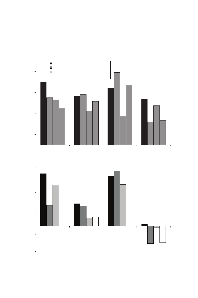
108 Hill, Holzer, and Chen

Figure 4.1 Effects of Household Structure on Outcomes, without and

with Enrichment, Neighborhood, and Parenting Controls

Panel A: High school dropout/GED (percentage points)

Panel B: Unmarried with a child (percentage points)

Without controls for enrichment, neighborhood, and parenting.

With controls for enrichment, neighborhood, and parenting.

High school dropout/GED

Unmarried with a child

Ever incarcerated

Mother never married

Mother had been married, no spouse in HH

Mother never married

Mother had been married, no spouse in HH

***

12.0

***

9.0 ***

8.6

***

7.0

***

12.5

***

5.0

***

9.8

3.6

***

7.9

***

4.3

***

6.6

***

3.6

0.0

2.0

4.0

6.0

8.0

10.0

12.0

14.0

16.0

Full sample

Blacks

Black males

Black females

***

12.0

***

9.0 ***

8.6

***

7.0

9.4

9.6

6.5

8.3

10.9

13.8

11.4

5.5

8.8

4.3

7.5

4.7

−6.0

−4.0

−2.0

0.0

2.0

4.0

6.0

8.0

10.0

12.0

14.0

Full sample

Blacks

Black males

Black females

***

12.5

***

5.0

***

9.8

3.6

5.4

4.8

2.0 2.2

11.9

13.1

9.9

−4.1

9.8

0.5

−0.3

−3.9

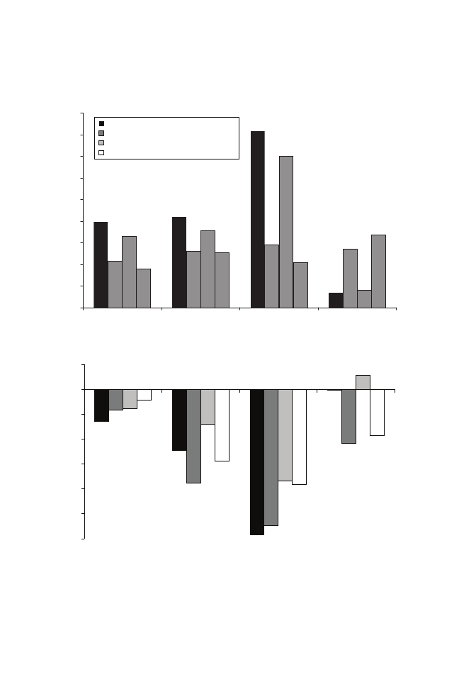
Other Correlates of Household Structure and Their Effects 109

NOTE: Coefficients are from Table 4.2. Regressions include respondents born between 1982 and 1984.

Regression variables were measured in Round 8 of the NLSY97, from October 2004 to July 2005.
Neighborhood, enrichment, and parenting variables are the variables reported in Table 4.1. Control

variables include respondent’s age at Round 8 interview, mother’s age when she had her first child,
whether mother is an immigrant, number of siblings in the respondent’s household at age 16, mother’s
educational attainment, mother’s hours worked, average family income at ages 14–15, and month of
Round 8 interview. Missing data dummies were included for all explanatory variables except for

race/gender. Statistical significance is denoted as follows: * p < 0.10; ** p < 0.05; *** p < 0.01.

Without controls for enrichment, neighborhood, and parenting.

With controls for enrichment, neighborhood, and parenting.

−6.0

−5.0

−4.0

−3.0

−2.0

−1.0

0.0

1.0

Full sample

Blacks

Black males

Black females

Mother never married

Mother had been married, no spouse in HH

Mother never married

Mother had been married, no spouse in HH

−1.3

−0.8−0.75

−0.4

−2.5

−3.7

−1.4

−2.9

−5.9

−5.5

−3.7 −3.8

−0.02

−2.2

−1.9

0.6

Panel D: Weeks worked (number of weeks)

Figure 4.1 (continued)

Panel C: Ever incarcerated (percentage points)

High school dropout/GED

Unmarried with a child

Ever incarcerated

Mother never married

Mother had been married, no spouse in HH

Mother never married

Mother had been married, no spouse in HH

***

12.0

***

9.0 ***

8.6

***

7.0

***

12.5

***

5.0

***

9.8

3.6

***

7.9

***

4.3

***

6.6

***

3.6

0.0

2.0

4.0

6.0

8.0

10.0

12.0

14.0

16.0

18.0

Full sample

Blacks

Black males

Black females

***

7.9

***

4.3

***

6.6

***

3.6

***

8.4

5.2

5.1

***

7.1

***

16.3

5.8

***

14.0

4.2

1.4

1.6

5.4

6.7

110 Hill, Holzer, and Chen

ternal knowledge of the youth’s companions tends to be associated
positively with educational outcomes (with relatively small substantive
effects) and negatively with incarceration (with moderate substantive
effects). Homes with well-kept interiors tend to be positively associated
with educational achievement and negatively associated with incarcera-
tion. For example, getting housework done is associated positively with
measures of education while eating dinner together is negatively associ-
ated with incarceration (though the estimated effects are substantively

small and not always statistically significant).

Finally, with regard to the neighborhood variables, both the per-

ceived absence of gunshots, reported by the respondent, and the impres-

sion of well-kept buildings, reported by the interviewer, are significantly
associated with educational outcomes and with some risky or illegal
activities, though substantively these effects are small.

The discussion above focuses on results for the full sample. With

regard to results for the black subgroups (black males, black females,
or both together), Table 4.3 indicates that the associations between hu-
man capital enrichment or neighborhood characteristics and the seven

outcomes are less often significant than in the full sample; this is due to
sample size limitations.

However, the parenting and home environment measures are jointly

significant in most equations for outcomes among the three subgroups,

just as they are for the full sample. More specifically (see Table A.5),

maternal knowledge of youth companions is often a significant predic-
tor, especially in the equation for incarceration; the estimated effects are
of similar or slightly smaller magnitudes than those of the full sample.
Having a well-kept interior and getting housework done are positively
related to college attendance and scoring well on the ASVAB.

In comparing black males and females, we see that the parenting

variables have significant effects on outcomes more frequently for
young black men than for young black women. For young black men,

the parenting and home environment measures are statistically signifi-
cant in equations for weeks worked, being a high school dropout or at-
tending college, ASVAB scores, and incarceration. Maternal knowledge

of companions is often significantly related to outcomes, especially for
dropping out of high school (a 1-standard-deviation increase is associ-
ated with a 5-percentage-point lower likelihood of dropping out).

Other Correlates of Household Structure and Their Effects 111

These results suggest that home environments and parental behav-

iors might importantly affect the propensity of young black men to fail
in and disconnect from school. Why these factors affect black males
more than black females or other youth remains unclear. Perhaps the
young men are more hurt by the absence of positive role models in
fathers, or perhaps their behavioral responses are more negative when
there is a lack of adequate supervision or structure in the home. More
research is undoubtedly needed to understand these effects more fully.
But, at a minimum, the apparently greater sensitivity of outcomes for
young black men to these measures of the home environment is im-
portant to consider when discussing potential remedies, as we do in
Chapter 5.

Can we make any causal inferences about these correlates of house-

hold structure and their estimated effects on behavior? As noted earlier
in the chapter, the human capital enrichment and neighborhood char-

acteristics are likely influenced by family income, though we control
for this in our regressions. Characteristics of parenting and the home
environment may be more directly a function of household structure.

We also do not necessarily attribute causality to any of the estimated

relationships between outcomes and the household characteristics. For
example, whether computer use really contributes to human capital and
labor market productivity has been questioned by DiNardo and Pischke
(1997) in their well-known response to Krueger (1993). Whether esti-

mates of “neighborhood effects” truly reflect causal impacts has long
been questioned (e.g., Jencks and Mayer 1990), while even the effects
of taking extra classes or lessons are subject to multiple interpretations.
For instance, taking classes might simply mean that young people are
more likely to be supervised by adults for some time period. If the

classes are remedial in nature, they might also reflect weaker underlying
academic skills of the student, and this might tend to offset any positive
effects of taking extra classes that might otherwise be observed.

Furthermore, the estimated associations likely also reflect endog-

enous relationships. For instance, in those cases where supportive
mothers are positively associated with various outcomes, the successful
youth might be more inclined to view their parents in a positive light
when they are successful than when they are not. On the other hand,
the growing interest in how a variety of noncognitive skills affect edu-

cational and employment outcomes (as reflected in the work of James

Table 4.3 Joint Significance of Human Capital Enrichment, Parenting, and Neighborhood Characteristics on

Outcomes

Set of variables
for which F-test
was conducted

Natural log of

hourly wage

Weeks

worked

High school

dropout/GED

Enrolled in

4-year college

or not enrolled,

bachelor’s

degree or more

ASVAB

Unmarried

with a child

Ever

incarcerated

Full sample

Human capital

enrichment variables

0.598

0.028

0.000

***

0.000

***

0.000

***

0.000

***

0.348

Parenting variables

0.324

0.723

0.000

***

0.000

***

0.000

***

0.319

0.000

***

Neighborhood variables

0.544

0.030

0.000

***

0.000

***

0.000

***

0.001

***

0.167

Observations

3,604

4,364

4,396

4,103

4,401

4,430

R-squared

0.071

0.075

0.185

0.263

0.387

0.154

0.291

Blacks

Human capital

enrichment variables

0.519

0.187

0.026

0.169

0.030

0.214

0.481

Parenting variables

0.744

0.086

0.001

***

0.000

***

0.000

***

0.569

0.026

Neighborhood variables

0.313

0.370

0.455

0.001

***

0.181

0.020

0.781

Observations

904

1,166

1,186

1,072

1,184

1,216

R-squared

0.092

0.102

0.213

0.197

0.304

0.130

0.374

1
13

Black males

Human capital

enrichment variables

0.601

0.791

0.115

0.012

0.101

0.612

0.520

Parenting variables

0.306

0.062

0.043

0.052

0.091

0.593

0.080

Neighborhood variables

0.236

0.057

0.504

0.008

***

0.098

0.020

0.500

Observations

429

557

568

543

566

598

R-squared

0.159

0.156

0.240

0.192

0.286

0.132

0.435

Black females

Human capital

enrichment variables

0.857

0.090

0.235

0.810

0.167

0.460

0.999

Parenting variables

0.854

0.780

0.016

0.002

***

0.006

***

0.212

0.407

Neighborhood variables

0.645

0.560

0.951

0.048

0.935

0.389

0.007

***

Observations

475

609

618

529

618

R-squared

0.107

0.142

0.248

0.263

0.357

0.176

0.199

NOTE: Cells show p-values for F

-tests of whether coefficients on variables in each indicated set were jointly equal to zero. Regressions

from Specification 4.1, whose household structure coefficients were reported in Table 4.2. The point estimates and standard errors for
each measure in each category are shown in Table A.5. The sample includes respondents born between 1982 and 1984. Variables were
measured in Round 8 of the NLSY97, from October 2004 to July 2005. Neighborhood, enrichment, and parenting variables are the vari-

ables reported in Table 4.1. Control variables include respondent’s age at Round 8 interview, mother’s age when she had her first child,
whether mother is an immigrant, number of siblings in the respondent’s household at age 16, mother’s educational attainment, mother’s
hours worked, average family income at ages 14–15, and month of Round 8 interview. Missing data dummies were included for all ex-

planatory variables except for race/gender. Statistical significance is denoted as follows:

p < 0.10;

p < 0.05;

***

p < 0.01.

SOURCE: Authors’ tabulations from NLSY97.

114 Hill, Holzer, and Chen

Heckman and others) is certainly consistent with many of our findings,
especially regarding parenting effects.

Despite these caveats, we are inclined to believe that some por-

tion of the associations we estimate between household characteristics
and outcomes is causal (though we cannot say how much). The ob-
served patterns of explanation are consistent with expectations: human
capital enrichment variables are more likely to affect educational out-
comes, whereas parental monitoring and structure in the home have an

influence not only on education but also on ever being incarcerated.
Furthermore, the estimated differences across demographic groups
are consistent with expectations: given the much greater propensity of
young black men to disengage from school than young black women,
the risky behaviors of young black males are more sensitive to environ-
mental and parental effects than those of young black females. Finally,
the estimates tend to be robust across multiple educational or behav-
ioral outcomes and across a variety of demographic groups. The overall
groups of human capital enrichment, neighborhood, and parental/home
environment variables are each likely to be more reliable and less sus-
ceptible to unobserved heterogeneity than are the component variables
within each category.

The relative robustness of the individual coeffi-

cient estimates to the various specifications we have tried also suggests
that some of these effects might be real as well.

At the same time, we acknowledge that our ability to fully account

for the observed effects of household structure remains limited in many
cases, and that the explanatory power of many groups of these variables
in our estimated equations is not high.

CONCLUSION

In this chapter we present descriptive statistics on eleven measures

of household characteristics. These measures—encompassing con-
structs of human capital enrichment, neighborhood quality, and par-
enting/home environment—are likely correlated both with household
structure and with seven different outcomes of young adulthood in the
areas of employment, education, and risky behaviors. We estimate re-
gression equations showing the extent to which controlling for these

Other Correlates of Household Structure and Their Effects 115

characteristics can account for the estimated relationships between
household structure and each of the outcomes, and we also consider the
effects of the household characteristics themselves on the outcomes.

Our results suggest the following:

• Human capital enrichment (as measured by the presence of com-

puters or dictionaries and attendance at extra lessons or classes)
and neighborhood safety are strongly associated with household
structure, and they are especially lacking in households headed
by never-married mothers.

• Parenting measures of maternal supportiveness and strictness,

maternal knowledge of youths’ companions, orderliness of the
home and timeliness of housework, and eating dinner together
are also associated with household structure, as single parents
have less orderly houses and know less about their children’s
companions.

• Human capital enrichment, parenting, and neighborhood char-

acteristics account for significant portions (generally 15-40 per-
cent) of the estimated effects of household structure on youth
outcomes, controlling for family income and a number of mater-
nal characteristics.

• Even after controlling for these additional measures, statistically

and substantively significant effects of household structure re-
main for a number of outcomes.

• Enrichment, neighborhood, and parenting measures themselves

have significant effects on youth educational and behavioral out-
comes.

• Estimated effects of household characteristics on outcomes for

blacks are similar to those for the full sample, while those es-
timated for black males are somewhat stronger than those for
black females.

These findings have mixed implications for our understanding of

how household structure affects outcomes observed among youth. On
the one hand, the correlations between household structure and enrich-
ment/neighborhood effects likely are largely spurious (except for those
operating through parental income, for which we have controlled) and
do not represent causal effects of family structure. On the other hand,

116 Hill, Holzer, and Chen

the fact that several parenting variables have significant effects on
educational and behavioral outcomes—and that the residual effects of
household structure after controlling for all these factors remain fairly
important—suggest some important causal effects of household struc-
ture as well.

These findings also have very mixed implications for the future

well-being of low-income youth growing up in single-parent families.
Youth growing up in single-parent households have less access to en-
richment materials or activities (at least as measured here) and are fre-
quently located in less safe neighborhoods than their counterparts from
two-parent families. At least on the dimensions measured here, these
youth face challenges in achieving academic success and avoiding risky
behaviors.

The results of this chapter suggest that a number of correlates of

more successful outcomes, however, can be managed by parents and
perhaps enhanced through appropriate policy interventions. These pre-
dictors seem to operate either through household structure or indepen-
dently of it. Providing more human capital enrichment in the home or
in school, improving neighborhood safety, and improving parental sup-
portiveness and supervision of youth might all improve the opportuni-
ties that young people have and thus contribute to their greater success
in terms of educational attainment and the labor market.

We consider these implications in greater detail in the concluding

chapter.

Notes

1. See BLS (2006) for a description of the general categories of such variables and

their availability in different rounds.

2. The bivariate correlations among these three measures ranged from 0.05 to 0.14.
3. The bivariate correlations among these measures ranged from 0.02 to 0.37, with

most being 0.13 or less.

4. The correlation between these two measures was 0.20.
5. Sample members were asked the number of days a week, on average, that they

did hear gunshots. So that higher values will indicate more positive neighborhood
environments, we subtract the responses from 7.

6. Sample weights are used in the summary statistics, but not in the regression

analyses.

7. The unweighted values of variables noted above were standardized to have a mean

Other Correlates of Household Structure and Their Effects 117

of 0 and a variance of 1. The weighted descriptive statistics shown in Table 4.1 do
not have a mean of 0.

8. In Chapter 3, the seven outcomes were analyzed for all NLSY97 sample members.

In the current chapter, these outcomes are analyzed for the subgroup of sample

members who were born in 1982–1984. Thus, the estimates for Specification 3.2
shown in Table 4.1 may be different from those reported in Chapter 3.

9. For example, blacks who lived with never-married mothers are 7 percentage points

less likely to attend a four-year college, and 7 percentage points more likely to be
incarcerated, compared to blacks who lived with both biological parents.

10. For example, each additional day that gunshots are not heard is associated with

a reduction in the probability of dropping out of high school or being unmarried
with a child by 1 to 2 percentage points, and it increases the probability of be-
ing enrolled in a four-year college by 1 percentage point. A 1-standard-deviation
increase in the degree to which buildings on the street are well-kept is associated
with a decrease in the probability of dropping out of 3 percentage points and an
increase in the probability of four-year college enrollment of 2 percentage points.

11. This assumes that the unobserved characteristics that are correlated with the in-

dividual variables in each group are not all the same and may tend to offset each
other.

12. More information is available from the authors on specifications in which these

variables have been entered separately or in various combinations.

119

Conclusion

Gaps in employment and education outcomes between young Afri-

can Americans and whites have persisted over the past several decades,

despite significant strides. Along some dimensions, such as employ-
ment and especially incarceration among young men, the racial gaps
have even widened.

Why do these gaps persist? One hypothesis suggests that the in-

creasing tendency of young blacks to grow up in female-headed house-
holds during the past few decades has contributed to the persistent and
even growing racial gaps in outcomes. While the trends in household

structure might themselves reflect other causes of worsening employ-
ment opportunities and outcomes among black men, these trends might
also contribute to a worsening set of outcomes among the next genera-
tion of youth.

In particular, young people growing up in single-parent families on

average have fewer financial resources, more stress, less supervision,
and fewer male role models than their counterparts who grow up with
both biological parents; thus, the widespread incidence of female head-
ship in black families might well contribute to less successful outcomes
for black youth.

Yet despite a substantial empirical literature on family structure and

its effects on youth outcomes, relatively little evidence to date exists on
how family structure affects a wide variety of outcomes among black
youth as compared with others, and for males versus females within
racial groups. Moreover, evidence on the mechanisms and pathways
through which these effects might occur has been somewhat limited.

In this book, we have used data from the NLSY—and especially the

1997 cohort—to explore these issues. We focus on a set of outcomes
for young people that include employment, school enrollment and at-
tainment, cognitive achievement, and participation in various risky or
illegal behaviors (such as bearing children outside marriage or com-
mitting a crime and becoming incarcerated). We estimate the statistical
relationships between these outcomes and the structure of households

120 Hill, Holzer, and Chen

in which youth grow up, controlling for a number of individual youth
and maternal characteristics.

We measure household structure—primarily at age 12—in a way

that captures some of the history of that structure as well as its current
status. We measure six categories of household structure, comparing
1) youth living with both of their biological parents (our reference
group) to those living with 2) never-married mothers, 3) previously
married mothers who now have no spouse in the household (i.e., those
divorced or separated), 4) mothers who have been previously married
but have a new spouse (i.e., are remarried), 5) biological fathers but not
their mothers, and 6) others (including grandparents, adoptive parents,
foster parents, or other arrangements). We present some evidence on the
stability of these arrangements over time, which motivates our decision
to focus on household structure and its history as of age 12, an age that
generally captures household structure during childhood as well as the
adolescent and teen years for most young people.

We include estimates of the effects of household structure on these

outcomes for youth, both without and with controls included for fam-
ily income, which is the most obvious mechanism through which such
effects might operate. We also estimate these equations separately for
blacks, and for black males and black females, to examine whether
household structure has different effects across these groups. We con-
sider the effects of household structure on race and gender differences
in each outcome, to infer the extent to which differences in household
structure can account for persisting racial gaps.

Of course, any estimated effects might not be truly causal, and

instead might reflect a range of other variables (like the family back-
grounds of the mothers themselves) that are correlated both with house-
hold structure and with outcomes but not measured in our data. We
do, however, include many control variables to mitigate concerns about
omitted variable bias; these include maternal employment, maternal

education, maternal age at first birth, immigrant status, and the sam-
ple member’s age and number of siblings. To further address concerns

about the identification of causal effects, we also estimate a series of

fixed-effects models in which we measure the effects of differences in
household structure on differences in outcomes, either between siblings
or over time for the same sample member.

Conclusion 121

After estimating the models that include controls for sample mem-

ber characteristics, maternal characteristics, and family income, we add
variables to the models to measure some of the mechanisms or pathways
through which household structure might affect youth outcomes. These
include a set of variables measuring human capital enrichment in the
home (the presence of computers or dictionaries as well as extra courses
or classes taken); another set measuring neighborhood environment, es-
pecially safety; and a third set measuring parental behavior and home
environment, including the degree of parental monitoring of friends, the
regularity with which work gets done or dinners are eaten together, and
the youth’s perception of parental strictness or supportiveness.

We consider the extent to which these measures account for ob-

served effects of household structure on youth and young adult out-

comes, and whether they themselves have significant effects—among
the full sample, separately for blacks, and separately for black males
and black females.

The remainder of this chapter summarizes our results and their im-

plications for further research and for policy.

SUMMARY OF EMPIRICAL FINDINGS

We begin in Chapter 2 by presenting data on the employment, edu-

cational, and behavioral outcomes of youth, separately by race and gen-
der, and looking at how at least some of these outcomes have evolved
over time. We compare data for similarly aged youth at comparable
points in the business cycle in the 1980s and 2000s.

We find, as expected, that educational and employment outcomes

continue to be lower for blacks and Hispanics than for whites. Young
women have generally made more progress in both education and em-
ployment than have young men in all racial groups over the past two

decades, and women now finish high school and enroll in college at
higher rates than men within each racial group.

But young black men, in particular, are falling even further behind

whites and Hispanics in a number of dimensions, and substantially be-
hind black women on measures of educational attainment and achieve-
ment. The greater participation of young blacks in risky behaviors—es-

122 Hill, Holzer, and Chen

pecially having children outside of marriage and (among men) engag-
ing in crime and becoming incarcerated—is noteworthy as well. For all
groups, but especially for young blacks, dropping out of high school
is associated with fewer weeks worked and a range of risky behaviors,
including crime and incarceration.

In Chapter 3, we turn our attention to the structures of households

in which youth live at age 12, and how these structures affect a range

of youth outcomes. We find, as expected, that young blacks are much
more likely to grow up in families without both biological parents than
are young whites. Indeed, the frequency of growing up without both
parents in the home is about 50 percent among youth overall and about
80 percent among young blacks. Family incomes of those growing up
without both biological parents are much lower than those with both
parents, especially among youth living with never-married mothers. But
other personal characteristics, such as maternal education, are highly
correlated with household structure as well, suggesting a variety of pos-
sible reasons (both causal and noncausal) for why outcomes of youth in
single-parent households might lag behind those of their counterparts.

When we examine the statistical relationships between household

structure and young adult outcomes, we find that these structures are
modestly related to labor market outcomes but more substantially re-
lated to youths’ educational attainment and achievement as well as to
nonmarital childbearing and incarceration. Controlling for household
income accounts for some—generally about a fourth to a half—of these
estimated effects, but by no means all of them.

Estimated effects are generally just as large among young blacks

as young whites, and often appear even larger among young black men
than young black women—especially on outcomes like weeks worked

and incarceration (though small sample sizes limit the statistical signifi-
cance of the estimated differences in most cases). Indeed, differences
in household structure seem to account for more than a third of the
higher black male rate of incarceration (relative to white males), more
than half of black males’ greater tendency to drop out of high school,
and most of their differences in college attendance in these equations.
Absent the changes in household structure over time, the rates at which
blacks drop out of high school would be several percentage points
lower than for whites (while their college attendance would be corre-
spondingly higher); the same is true of their tendencies to have children

Conclusion 123

outside of marriage and to become incarcerated. A set of fixed-effects
models, both between siblings and over time for the same individuals,

also shows some significant effects of household structure on outcomes,
suggesting at least partly causal effects of the former on the latter.

In Chapter 4, we seek to establish more of the mechanisms and

pathways (besides household income) through which the effects of

household structure on outcomes might work. We find that measures
of human capital enrichment and neighborhood safety are highly cor-
related with family structure, in that the highest rates of enrichment and
safety are observed among those living with both biological parents
and the lowest among those living with never-married mothers. Parent-
ing behaviors are also somewhat correlated with household structure,
as single mothers are perceived by youth as being stricter, monitoring
youth behaviors and peers less closely, and getting housework done and
having dinner together less frequently.

The data also show that human capital enrichment, neighborhood

safety, and parenting behaviors account for fairly substantial portions
(15 to 40 percent) of the estimated effects of household structure on

youth outcomes. All three sets of variables have jointly significant es-
timated effects on youth outcomes, with the human capital measures
having somewhat stronger effects on education and the neighborhood
and parenting measures mattering a bit more for behavioral outcomes.
Again, estimated effects for young black men are as strong as or stron-
ger than those for young black women or for whites and Hispanics.

To what extent are all of these estimated effects on youth out-

comes—including those for household structure as well as those for the

mediating variables—truly causal, rather than just reflecting omitted
variables that we cannot measure? Regarding the estimated effects of
household structure, we note that the maternal characteristics for which
we control (including employment, education, age, nativity, and num-
ber of children) are more extensive than those included in many other

studies. Furthermore, our fixed-effects estimates, both across siblings
and over time for the same individual, also suggest that some parts of
the estimated household effects are causal, even though these tests have
some major practical limitations that likely cause them to understate the
effects of changes in household structure on outcomes.

Whether or not the estimated effects of human capital enrichment,

neighborhood environment, and parenting variables themselves are also

124 Hill, Holzer, and Chen

causal is harder to establish. Nevertheless, these estimates are quite ro-
bust across many different outcomes and different race or gender groups
among young adults. The particular pattern of estimated effects—a pat-
tern of human capital variables affecting education outcomes strongly
while neighborhood and parenting variables affect nonmarital births
and incarceration relatively more—is consistent with a causal interpre-
tation. And considering the sets of variables as constructs of interest
(instead of interpreting each variable separately) also likely strengthens
the interpretation of the construct as a whole as being causal and weak-
ens the likelihood that the sets of variables are fully driven by their cor-
relations with omitted factors, as we note in Chapter 4.

Summing Up

In all, our analysis suggests that black youth—and especially young

black males—continue to lag behind whites (and Hispanics as well)
quite dramatically on educational, employment, and behavior outcomes,
and in some cases (such as employment and incarceration) they are fall-
ing even further behind. Almost certainly, the fact that so many of these
young people grow up in families without both biological parents—and
especially with never-married mothers—has impeded progress along
many dimensions and contributed to worsening outcomes in some cases.
All else being equal, the high incidence of single parenthood in the
black community has limited the incomes of the households in which
young people grow up, and also the ability of parents to provide stable
and orderly environments in which they can monitor the activities of
their youth and guide them appropriately.

And the apparently larger effects of single-parent households on

some outcomes of young black males than on those of young black fe-
males suggests the particularly important role that household structure
might play in generating poor employment and behavioral outcomes for
this group. We can only speculate about exactly why this is true. Be-
havioral issues during adolescence and the teen years for young males
in general seem more serious than those for young females, especially
in low-income families, and a gender gap in academic performance and
achievement has now appeared among all groups.

But, especially among lower-income black families and neighbor-

hoods, the effects of household structure seem to matter more for males.

Conclusion 125

Perhaps this reflects the impact of a lack of positive male role mod-
els and mentors for this group, or the lack of strong paternal supervi-
sion on their behavior. Alternatively, the interactions between single
mothers and their sons might be more strained than between mothers
and their daughters. Positive impacts of programmatic treatments for
young girls but not boys have been seen in other contexts as well, such
as the Moving to Opportunity experiments (though the effects of New
Hope employment assistance were stronger for boys). Whatever their
causes, the particularly negative impacts on outcomes of young black
males are noteworthy and require further attention by researchers and
policymakers.

At the same time, however, it is also clear that household structure

does not fully account for the continuing racial gaps in most of these
outcomes. For instance, racial gaps in employment, childbearing outside
marriage, and incarceration between black (male) youth and others per-
sist even after controlling for single parenthood. Furthermore, the disad-
vantages caused by single parenthood are compounded by the lower edu-
cation levels and earnings of these parents, the lack of cognitive enrich-
ment in their homes, and their residence in less safe neighborhoods—all
of which do not appear to be caused by single parenthood per se.

In sum, many young blacks and especially black males are swim-

ming against the tide as they grow up: they face a multitude of dis-
advantages associated with (causally or otherwise) coming of age in
single-parent families that limit their opportunities in life. These dis-

advantages reflect a wide range of factors in the home, and are then
compounded by various neighborhood effects, presumably in school
and out of it. Accordingly, the analysis here implies that a wide array of
policy responses is necessary to offset the full range of disadvantages
these young people face as they grow up. Identifying policies that can
offset these many disadvantages in cost-effective ways is the challenge
that we now must address.

IMPLICATIONS FOR FURTHER RESEARCH

Our analysis strategy has involved the estimation of regression

models that include an extensive set of controls and the estimation of

126 Hill, Holzer, and Chen

fixed-effects models (both for siblings and for individuals over time).
In some cases, these strategies eliminate the effects of household struc-
ture (for example, in the cases of wages and hours worked). But for
other outcomes, effects of household structures on outcomes remain
(for example, in the cases of educational attainment, being unmarried
with a child, or ever having been incarcerated). Such persistent effects
of household structure in these cases lead us to conclude cautiously that
the effects of household structure that we estimate are at least partly

causal. Our fixed-effects estimates tend to reinforce this view.

Yet the estimation strategies that we use cannot convincingly elimi-

nate the possibility that omitted factors that are correlated both with
household structure and with these outcomes are actually driving some

of these results. Thus, we cannot claim definitively that our estimated

effects of household structure are truly causal. A first implication for
further research is thus to pursue additional estimation strategies that
can identify causal effects of household structure on the types of out-
comes we examine in this study. These might include instrumental vari-

ables or other variants of the fixed-effects models estimated here.

In Chapter 4, we show estimates of the effects of sets of human cap-

ital enrichment, neighborhood safety, and parenting/home environment
characteristics on seven outcomes. These effects are estimated from
models with an extensive set of controls. While the estimates of these
variables seem somewhat robust across different samples, and while our
results are consistent with what one might expect (for example, as with
the human capital enrichment variables related to educational outcomes
and with the parenting variables related to risky behavior outcomes),
claims about causality are weaker here than for household structure and
require even more attention.

A second implication for further research, then, is the need for iden-

tifying the causal effects of the types of enrichment, neighborhood, and
parenting variables that we examine in this paper. More broadly, devel-
oping a fuller understanding of the mechanisms through which house-
hold structure might affect youth outcomes, and also of the family and
neighborhood factors that might tend to offset these effects, remains a
high priority for research. Better understanding of the timing of these
effects and of how they vary across different household structures (in-
cluding families with stepparents and cohabiting adults), is in order as
well. And understanding more about the role of noncustodial fathers,

Conclusion 127

and the impact of their relationships with youth on outcomes, is impor-
tant too.

Research that addresses causality and robustness will provide fur-

ther confidence for policy prescriptions like the ones offered below,

which are designed to influence household structure and its correlates
and to improve outcomes for all young adults, but especially for young
minorities.

POLICY IMPLICATIONS

Overall, it seems that the goals of public policy with respect to the

household structures in which young people grow up should be two-

fold: first, to reduce the frequency of young people growing up with
single parents; and, second, to improve opportunities and outcomes for
young people who continue to live in such homes.

Given those goals, what might such a set of policies include? To

what extent should we target the behaviors and outcomes of single par-
ents versus those of their children and youth? And how much effort
should be placed on the prevention of single parenthood through broad
improvements in opportunity for young people, as opposed to efforts to
offset its negative effects once it has occurred?

Broadly, our evidence implies the need for the following set of five

policy efforts:

1) Discouraging single parenthood—by promoting marriage or

discouraging unwed pregnancy, whenever possible;

2) Raising the incomes of unmarried working parents—either by

improving their earnings capacity or by further supplementing
their low earnings in a variety of ways;

3) Improving the schooling and neighborhood environments of

youth—to offset early disadvantages and prevent them from
worsening over time;

4) Improving supervision of youth and parenting—in programs

and at home, both among custodial and noncustodial parents;
and

128 Hill, Holzer, and Chen

5) Limiting racial disparities in employment and crime/incarcer-

ation among youth more generally—through a wide range of
general programmatic and policy efforts.

But do we know how to accomplish these goals cost-effectively?

Our evidence of what works and what doesn’t in each area is limited.
Absent such clear evidence, we need a comprehensive effort that gen-
erates continuing research and evaluation in each area, while we ex-
periment with a broad range of programmatic and policy efforts in

the meantime. We briefly discuss some possible options, and what we
know and don’t know about their cost-effectiveness, for each policy
goal below.

1) Discouraging Single Parenthood

Marriage promotion received attention as a policy priority for the

Bush administration, particularly through its Healthy Marriage Initia-
tive. Some evidence exists that there are approaches that successfully
promote marriage among middle-class couples, but virtually no evi-
dence is available pointing to what, if anything, works for promoting
healthy marriages among the poor (Dion 2005; Ooms 2007). Perhaps
such information will emerge from the current round of demonstration
projects funded by the U.S. Department of Health and Human Services
in this area. We remain somewhat skeptical that enough is known about

how to influence the marital choices of low-income young people. We
also doubt that the kinds of interventions used in these efforts (like coun-

seling) are sufficient to overcome the huge barriers to marital matching
and success that such young people face, especially in the form of low
employment and earnings capacities, and the stresses on marriage that
these constraints generate.

Furthermore, among families where the children have the same

never-married mother but each has a different biological father, the
exact candidate for marriage to the mother is unclear, and some off-
spring will no doubt become stepchildren of these new fathers, which
is a much more ambiguous outcome from the children’s point of view
(Acs 2006). Promotion of marriage before such circumstances develop
would likely be more successful than afterwards, if at all possible.

While the cost-effectiveness of various marriage promotion options

remains quite uncertain, we have a somewhat greater understanding of

Conclusion 129

how to deter (or at least delay) childbearing among those who are un-
married, especially teens. While any one option in this area, such as
abstinence-only, is unlikely to be effective, strategies that combine mul-
tiple approaches of education, community service activities, messages
through the news media, and youth development appear somewhat
more successful (National Campaign to Prevent Teen and Unplanned
Pregnancy 2008).

There is also some evidence to date that improved enforcement of

child support obligations on noncustodial fathers tends to discourage
unwed pregnancy (Pirog and Ziol-Guest 2006). On the other hand, cer-
tain aspects of current child-support enforcement efforts appear to have
some negative unintended consequences on the employment and par-
enting of poor noncustodial fathers.

Finally, perhaps the most effective strategies to further marriage

and prevent unwed pregnancy would involve improving the earnings
and employment prospects of young African American men, as we dis-
cuss more fully below.

2) Raising Incomes among Unmarried Working Poor Adults

Because lower family income accounts for at least some part of

the negative effects of single parenthood on youth outcomes, raising
the family incomes of working single parents might be another way of
offsetting these negative effects. While virtually no one advocates the
resurrection of welfare policies that simply provide cash income main-
tenance to the poor (without being tied to work), further supplementing
the incomes of working-poor adults might be helpful. Indeed, evidence
from a variety of experimental efforts that supplemented the earnings
of low-income welfare mothers shows that earnings supplements for
low-income parents can raise achievement among children and youth
(Morris, Gennetian, and Duncan 2005).

The Earned Income Tax Credit (EITC) is the most obvious vehicle

for expanding the incomes of the working poor. The current federal
credit, which is worth approximately $4,800 at its peak for low-income
working parents with two or more children, clearly encourages greater
work effort while providing more income to the poor (Meyer and Rosen-
baum 2001). A number of states also supplement the federal EITC with
their own tax credits.

130 Hill, Holzer, and Chen

But the federal EITC and state credits might be amended in a num-

ber of ways. For one thing, the current phaseout rate (at 21 percent of
earnings above roughly $16,000 for families with two children) might
discourage work among two-parent families or discourage marriage, as
both tend to raise family income and therefore reduce eligibility for the
EITC. Reducing the phaseout rate, raising the threshold at which phase-
out begins, or counting only parts of a spouse’s earnings in calculating
household income would provide more income to these families while
reducing taxes on both work and marriage. Greater cash payments to
those with three or more children, or to those with just one child, might
well be considered too.

And, given the poor wages and employment incentives for low-

income young men (especially those who are noncustodial fathers), an
expansion of the EITC—either to childless adults in general or to non-
custodial fathers in particular (for those who are at least keeping up

with their current child support orders)—might be justifiable. Indeed,
the State of New York has recently undertaken the latter approach,
whereas several analysts have advocated some version of the former
(Berlin 2007; Edelman, Holzer, and Offner 2006).

And there are a number of other ways of supplementing the earn-

ings of the working poor that might also be particularly helpful to chil-

dren and youth in these families. Specifically, policies that extend paid
parental and medical leave to low-income working parents, as well as
child care and health insurance, are likely to relieve stress and generate
gains for youth in these families (Waldfogel 2007).

In addition, a variety of approaches that would raise the earnings ca-

pacity of working poor adults need to be explored and more rigorously
evaluated. A lengthy literature already exists on the cost-effectiveness
of job training for disadvantaged youth and adults, which mostly shows
the modest effectiveness of modest programs for adults. But newer ap-
proaches have been developed in recent years that involve some com-
bination of 1) education or training, usually at community colleges,
perhaps targeted at growing sectors of the economy (like health care,
construction, and the like) that provide above-minimal wages to non-
college workers; 2) a range of work supports, including child care as-
sistance and transportation as well as stipends for any training period;
and 3) job placement efforts that seek to match these workers with bet-
ter employers and jobs. These efforts would all be coordinated by labor

Conclusion 131

market intermediaries—third-party groups (such as community-based

organizations or other for-profit or nonprofit associations) that bring
together workers, employers, training providers, and public supports.

Indeed, one recent proposal (Holzer 2007) calls for the federal gov-

ernment to fund competitive grants to states and local areas for build-
ing such “advancement systems.” States would be required to carefully
measure performance while more rigorous evaluation evidence on these
approaches was generated, and renewal of these grants over time would
depend on states incorporating any knowledge that was generated from
these performance measures and from evaluation.

Finally, efforts that directly try to raise wages on the demand side

of the labor market for low-income workers might be included here as
well (Bartik 2001; Holzer 2007). These would include occasional in-

creases in the minimum wage (or indexing it to inflation), legal efforts
to make it easier for low-wage workers to unionize, and local economic
development efforts (like tax credits and grants) that particularly re-
ward the generation of higher-wage jobs. The potential effects of higher
minimum wages and unionism on employment rates must, of course, be
considered in any such efforts.

3) Improving Schooling Options and Neighborhood Safety for
Poor Youth

Since the negative effects of single parenthood on youth seem clear-

est for academic outcomes, such as completing high school and enrolling
in college, and since these effects operate through (or are compounded
by) weak academic enrichment opportunities in the home and residence
in unsafe neighborhoods, policies might be undertaken to directly com-
bat these problems by providing for more academic opportunities and
improving neighborhood quality for low-income and minority young
people, especially in single-parent families.

Of course, exactly how to accomplish these worthy goals can be

(and frequently is) heavily debated elsewhere. The returns to high-
quality early childhood education efforts, despite their high cost, have
been quite well established (Ludwig and Sawhill 2007), and the returns
to universal prekindergarten programs in Oklahoma and elsewhere look
especially strong for lower-income students and minorities (Gormley
and Gayer 2005). But large questions remain about whether the stron-

132 Hill, Holzer, and Chen

gest programs (like the Carolina Abecedarian Project and the High/
Scope Perry Preschool Program) can be replicated and scaled up, and
whether these effects tend to fade with time. The cost-effectiveness of
many other approaches in the K-8 years—such as smaller class sizes,
school choice efforts, and high-stakes testing—are even less clear. Ef-
forts to improve teacher quality in poor areas (Bendor, Bordoff, and
Furman 2007) are less controversial and could have important effects
on educational quality for poor children. Desegregation of schools
might also tend to limit racial gaps in student achievement (Card and
Rothstein 2005; Weiner, Lutz, and Ludwig 2006), but these efforts are
much more politically controversial, and their legal status has been cast
into doubt by recent court rulings.

But as low-income youth enter their high school years in any loca-

tion, it is desirable that they should face a better range of pathways
to success in postsecondary education, employment, or both. Some of
these pathways could be based on high-quality Career and Technical
Education (CTE) along with early labor market activity; indeed, we
have fairly strong evidence on the cost-effectiveness of Career Acad-
emies and Tech Prep in improving postschool employment outcomes
for at-risk youth (Lerman 2007). Others involve improving access to

higher education through better financial aid and other supports, as in
Project Opening Doors, which has generated some positive results in
recent evaluations (Brock and Richburg-Hayes 2006). Some proposals
would improve Pell grant availability and reduce the complexity of the
application process (Dynarski and Scott-Clayton 2007). Direct efforts
to reduce the very high dropout rates that characterize high schools in
many poor urban and rural areas must also be pursued, even while ef-
forts to evaluate what works in this area continue (Pennington 2006).

How might we improve the quality of neighborhoods in which

low-income and minority young people grow up? Turner, Popkin, and
Rawlings (2008) review what we know about legal and programmatic
efforts to improve housing or neighborhood quality among poor minor-
ities and to reduce residential segregation. The Moving to Opportunity
(MTO) experiments seem to have mixed effects, which are generally
more positive for female than male youth (Kling, Ludwig, and Katz
2005). And we know fairly little about the cost-effectiveness of efforts
to improve home environments by supporting greater asset develop-

Conclusion 133

ment, particularly home ownership, among the poor (McKernan and
Ratcliffe 2007).

Other efforts to improve services to youth at the community level,

such as the Youth Opportunity grants recently distributed by the U.S.
Department of Labor or the Harlem Children’s Zone, seem promising
(Edelman, Holzer, and Offner 2006) but also require more rigorous

evaluation. These, of course, are specific approaches within the broader
category of “youth development” programs at the community level
that might well decrease a variety of negative behaviors and outcomes
among youth and improve their education and earnings outcomes over
time (Eccles and Gootman 2002).

4) Improving Supervision of Youth and Parenting

To the extent that low-income single parenthood may result in less

positive parenting and home environments (perhaps associated with the
greater instability and stresses that are prevalent in many such homes),
greater provision of child care or after-school care as well as direct par-
enting supports might be helpful.

While some analysts (e.g., Besharov and Samari 2001) argue that

the provision of child care for low-income working parents is already
ample, this view is disputed elsewhere (e.g., Greenberg, Ewen, and
Matthews 2006). The need to improve the quality of such care seems
less controversial, though exactly how to do so remains open to ques-
tion (Blau 2001). Improving access to center-based care (as well as
early childhood education) seems to be one route to improving child
care quality.

Also, youth supervision might be improved through the kinds of

positive youth development efforts cited above, including programs
like Boys and Girls Clubs of America, and also through a variety of
after-school programs, such as those supported by the 21st Century
Community and Learning Centers. While the evaluation evidence on the
latter efforts has been somewhat disappointing to date (James-Burdumy
et al. 2005), efforts to identify cost-effective strategies in this area
should continue.

Is it possible to directly improve parenting by other means, such as

interventions for children that include their parents as well? Head Start
attempts to do so (Schumacher 2003), though whether it is successful

134 Hill, Holzer, and Chen

is open to debate. Other efforts to directly involve parents and improve
their skills at rearing children and youth have appeared in a variety
of contexts, such as the Comer School Development Program (Comer
2004) and the Infant Health and Development Program (Brooks-Gunn,
Liaw, and Klebanov 1992). Indeed, rigorous evaluations have found the
latter to be successful.

In terms of improving parenting, additional efforts could focus on

encouraging noncustodial fathers to have more active and responsible
involvement with their children. Previous research has suggested im-

portant potential benefits in this approach (Billingsley 1992; Clayton,
Mincy, and Blankenhorn 2003; Mincy 1994).

Indeed, effective father-

hood programs might be considered complementary with, rather than
substitutes for, marriage promotion programs (Ooms et al. 2006).

But what is needed to encourage more effective fatherhood? At

a minimum, it would seem that improving employment opportunities
for noncustodial fathers would be a critical component of any such ap-
proach. Among low-income noncustodial fathers, employment rates
and earnings levels are extremely low (Mincy and Sorensen 1998), sug-
gesting perhaps limited earnings capacity with which to support non-
custodial children. At the same time, for those who are in arrears on
child support payments (particularly those who have been incarcerated),
the incentive to accept low-wage employment is very low, because the
implicit tax rates on these earnings are so high (up to 50 percent), and
much of the money collected is not even passed through to families
(Holzer, Offner, and Sorensen 2005).

Thus, improving employment among low-income noncustodial fa-

thers might require some reforms in the child support system, along with
employment and training assistance for those with limited employment
options on their own (Bloom and Butler 2007; Edelman, Holzer, and
Offner 2006). Counseling and peer support groups for absent fathers
are also frequently included in such efforts. With respect to the cost-
effectiveness of these programs, the rigorous evaluation of the Parents’
Fair Share program (Miller and Knox 2001) found that the fatherhood
efforts contained in that program modestly improved the quality of par-
enting among noncustodial fathers but not their employment rates or
child support payments. A more effective approach might require more
rigorously enforced child support payments as well as more generously
supported transitional employment opportunities and additional subsi-

Conclusion 135

dies, as were provided in the New Hope demonstration in Milwaukee
(Duncan, Huston, and Weisner 2007; Primus 2006).

Finally, because so many low-income noncustodial fathers also

have criminal records—especially among African Americans—efforts
to raise their employment level must address the particular barriers
faced by this group. These barriers are substantial on both the demand
side of the labor market (employer attitudes and hiring behaviors may
discriminate against those with criminal records) and the supply side
(the potential workers may lack the requisite skills), as discussed by
Holzer (2009). Rigorous evidence on cost-effective approaches here,
too, is limited.

But in addition to funding successful reentry programs,

reducing the legal barriers to employment among those with criminal
records might be important as well (Holzer, Raphael, and Stoll 2003).

5) Limiting Racial Disparities in Employment and Crime/
Incarceration among Youth

The evidence presented in this book shows that, even after account-

ing for differences in household structure, racial gaps remain in some
outcomes between whites and blacks, especially among young men.
The most striking gaps—in employment levels and incarceration—are
partly, but not fully, accounted for by racial gaps in education and basic
skills. These discouraging outcomes in turn likely contribute to high
rates of single parenthood in the black community, as fewer men are
considered worthy prospects for marriage by their potential mates, and
fewer are themselves interested in marriage or parenting, given their
circumstances.

We have reviewed a variety of efforts above that would ultimately

improve the employment prospects of young black men. Some would
work through early schooling and employment activities, while oth-
ers would target working poor adults or hard-to-employ noncustodial
fathers and exoffenders. As we also noted above, broad-based efforts
to improve opportunities for youth should seek to reduce racial segre-
gation in schools and neighborhoods. Additionally, they should target
the labor market discrimination that still exists toward black men of all
ages (Holzer 2006; Pager 2007), either through improved enforcement
of Equal Employment Opportunity (EEO) laws or better dissemination
of information on applicant quality.

136 Hill, Holzer, and Chen

Promising employment programs for minority out-of-school youth,

such as YouthBuild or the Youth Service and Conservation Corps, could
be funded at much greater levels than they are currently (Edelman,
Holzer, and Offner 2006), even while efforts continued, through rig-
orous evaluation, to determine exactly what approach is most cost-
effective. At the same time, community-based efforts to combat the

alienation and resentments of youth which find their expression in an
“oppositional culture” (Mead 2006) could also gain more support. And
as a society we might rely less heavily on incarcerating young men
for nonviolent drug offenses, as we did in the past (Raphael and Stoll
2007).

Given the enormous social costs associated with the status quo (Hol-

zer et al. 2007), a wide variety of efforts to combat low employment

and high incarceration for this population are clearly justified—even if

they require some significant expenditure of resources, and even if our
knowledge of their cost-effectiveness remains imperfect.

Notes

1. Berlin’s (2007) proposal would provide tax credits to low-earning adults regard-

less of their family income, in order to avoid marriage penalties, while Edelman,
Holzer, and Offner (2006) call for more limited payments that would still depend
on family income. To avoid large marriage penalties, the latter propose to only
count half of a second earner’s income when computing eligibility. Berlin’s pro-
posal would likely cost more than $30 billion a year, while Edelman, Holzer, and
Offner estimate that theirs would cost about $10 billion.

2. The training models for working poor adults that target the demand side of the

labor market more clearly include sectoral training, tax credits for incumbent
worker training, and building career ladders, either within smaller establishments
(like nursing homes) or across them. See Holzer and Martinson (2005) and Oster-
man (2007).

3. In particular, the U.S. Supreme Court struck down voluntary school desegregation

efforts in Seattle and Louisville in rulings delivered on June 28, 2007. Justice An-
thony Kennedy, who was the swing vote in each of these 5-4 rulings, has indicated
he may support certain desegregation efforts that do not target individual students
by race.

4. Our own tabulations from the NLSY97 (not reported here) also document the

very limited involvement of never-married fathers with their noncustodial chil-
dren relative to fathers in every other group. These, too, suggest some important

potential benefits to improving fathering practices among this group.

Conclusion 137

5. Preliminary results from MDRC’s evaluation of the Center for Employment

Opportunities (or CEO) in New York suggest major reductions in recidivism
from efforts to provide services and transitional jobs to ex-offenders right after
release from prison, though impacts on employment beyond the program were
disappointing.

6. In particular, labor market intermediaries might be able to reduce statistical dis-

crimination in hiring by providing employers with information about job appli-

cants that the employers themselves might not find. For evidence on how infor-
mation from background checks can actually reduce discrimination against black
men, see Holzer, Raphael, and Stoll (2006).

139

Appendix A

Background Tables

140

Table A.1 Recursive Employment and Education Regressions for Black Males

Natural log of hourly

wage, past year

Weeks worked, past year

High school dropout,

Nov. 2004

Model 1

Model 2

Model 3

Model 1

Model 2 Model 3 Model 1

Model 2

Model 3

Age

0.050

***

0.045

***

0.044

***

1.639

***

1.269

***

1.402

***

0.003

−0.003

(0.011)

(0.483)

(0.489)

(0.493)

(0.011)

(0.009)

Education level

Not enrolled, high school dropout

or GED

−0.201

***

−0.165

−15.434

***

−12.701

***

(0.073)

(0.076)

(3.419)

(3.541)

Not enrolled, high school degree

−0.074

−0.056

−8.291

***

−7.222

(0.069)

(0.072)

(3.156)

(3.224)

Not enrolled, some college or

associate’s degree

−0.039

−0.017

−1.914

−0.964

(0.070)

(0.072)

(3.003)

(3.109)

Enrolled, two-year college

−0.176

−0.157

−7.881

−7.110

(0.074)

(0.075)

(3.963)

(4.102)

Enrolled, four-year college

−0.145

−0.137

−10.364

***

−9.643

***

(0.081)

(0.083)

(3.446)

(3.515)

GPA in high school

−0.038

−0.048

0.160

−0.106

−0.228

***

−0.177

***

(0.032)

(0.033)

(1.312)

(1.319)

(0.024)

(0.025)

ASVAB percentile

0.045

0.054

***

0.966

1.111

−0.115

***

−0.090

***

(0.019)

(0.020)

(1.012)

(1.021)

(0.018)

Unmarried and has children

0.026

1.367

0.102

***

(0.036)

(1.596)

(0.033)

Risky behaviors prior to age 18

Drank alcohol

−0.002

−1.965

−0.044

(0.033)

(1.551)

(0.028)

141

Smoked cigarettes

−0.037

2.001

0.080

***

(0.035)

(1.525)

(0.029)

Smoked marijuana

−0.023

−2.372

0.038

(0.033)

(1.687)

(0.033)

Ever stole something worth $50 or

more, joined a gang, attacked
someone, or was arrested

−0.021

−1.576

0.061

(0.033)

(1.583)

(0.027)

Ever incarcerated

−0.031

−6.593

***

0.222

***

(0.048)

(2.165)

(0.047)

Constant

1.009

***

1.312

***

1.356

***

−5.181

18.685

22.525

0.530

0.650

0.468

(0.287)

(0.325)

(0.344)

(15.856)

(17.726)

(18.209)

(0.322)

(0.308)

(0.298)

Observations

679

910

923

R-squared

0.051

0.093

0.106

0.025

0.097

0.127

0.029

0.247

0.324

NOTE: Robust standard errors are shown in parentheses. Variables were measured in Round 8 of the NLSY97, from October 2004 to July

2005. Dummy variables controlling for month of interview are included but not reported. Missing data dummies were included for all

explanatory variables except for race/gender. Statistical significance is denoted

p < 0.10,

p < 0.05, and

***

p < 0.01.

The omitted educational category in the regression is “not enrolled, some college or college degree.”

142

Table A.2 Recursive Employment and Education Regressions for Black Females

Natural log of hourly

wage, past year

Weeks worked, past year

High school dropout, Nov. 2004

Model 1

Model 2

Model 3

Model 1

Model 2

Model 3

Model 1

Model 2

Model 3

Age

0.067

***

0.058

***

0.060

***

1.528

***

1.144

***

1.174

***

−0.015

−0.012

−0.015

(0.010)

(0.011)

(0.427)

(0.437)

(0.443)

(0.008)

(0.007)

Education level

Not enrolled, high school dropout

or GED

−0.320

***

−0.297

***

−14.749

***

−12.892

***

(0.078)

(0.081)

(2.834)

(3.009)

Not enrolled, high school degree

−0.264

***

−0.256

***

−7.828

***

−7.246

***

(0.068)

(0.071)

(2.317)

(2.411)

Not enrolled, some college or

associate’s degree

−0.220

***

−0.211

***

−5.076

−4.803

(0.068)

(0.071)

(2.232)

(2.300)

Enrolled, two-year college

−0.266

***

−0.259

***

−6.592

−5.873

(0.081)

(0.084)

(2.777)

(2.868)

Enrolled, four-year college

−0.271

***

−0.273

***

−6.687

***

−6.740

***

(0.074)

(0.076)

(2.311)

(2.323)

GPA in high school

−0.068

−0.062

1.905

1.718

−0.181

***

−0.143

***

(0.030)

(0.031)

(1.154)

(1.169)

(0.021)

(0.022)

ASVAB percentile

0.114

***

0.105

***

2.489

***

2.468

***

−0.090

***

−0.082

***

(0.021)

(0.022)

(0.899)

(0.925)

(0.016)

Unmarried and has children

−0.044

−0.905

0.061

***

(0.031)

(1.353)

(0.023)

Risky behaviors prior to age 18

Drank alcohol

0.009

−0.263

−0.029

(0.032)

(1.419)

(0.025)

143

Smoked cigarettes

−0.002

−0.636

0.103

***

(0.031)

(1.462)

(0.026)

Smoked marijuana

0.044

1.490

0.063

(0.034)

(1.566)

(0.029)

Ever stole something worth $50 or

more, joined a gang, attacked
someone, or was arrested

0.015

−2.545

0.042

(0.029)

(1.303)

(0.022)

Ever incarcerated

−0.165

−7.309

0.295

***

(0.096)

(3.935)

(0.075)

Constant

0.472

1.068

***

0.938

***

15.320

26.010

35.927

***

0.701

***

0.858

***

0.693

***

(0.297)

(0.341)

(0.356)

(10.246)

(11.907)

(12.618)

(0.259)

(0.246)

(0.236)

Observations

814

1,031

1,041

R-squared

0.068

0.137

0.151

0.027

0.113

0.127

0.022

0.252

0.318

NOTE: Robust standard errors are shown in parentheses. Variables were measured in Round 8 of the NLSY97, from October 2004 to July

2005. Dummy variables controlling for month of interview are included but not reported. Missing data dummies were included for all

explanatory variables except for race/gender. Statistical significance is denoted

p < 0.10,

p < 0.05, and

***

p < 0.01.

The omitted educational category in the regression is “not enrolled, some college or college degree.”

144

Table A.3 Household Structure Stability of Respondents between Ages 2 and 12 (%)

At age 2, sample member

lived with:

Both

biological

parents

Mother,

never

married

Mother,

had been

married,

no spouse in

household

Mother and

her spouse

Father

Other

Total

Sample size

At age 12, sample member

lived with:

Both biological parents

98.13

0.00

0.24

0.48

1.15

1.30

51.42

3,535

Mother, never married

0.01

95.34

0.00

0.59

5.62

653

Mother, had been married,

no spouse in household

0.01

0.00

42.66

42.78

1.29

2.41

14.75

1,139

Mother and her spouse

0.08

0.00

52.59

52.56

1.46

5.91

18.28

1,394

Father

0.13

0.11

0.93

2.05

92.93

2.63

4.62

341

Other

1.64

4.55

3.57

2.12

3.18

87.16

5.32

479

Total

100

7,541

Sample size

3,583

679

845

1,794

314

326

7,541

NOTE: Proportions are calculated from the NLSY97 cohort using Round 8 sample weights.

145

Table A.4 Household Structure Stability of Respondents between Ages 12 and 16

At age 12, sample member

lived with:

Both

biological

parents

Mother,

no other

parent

Mother and

her spouse

Father

Other

Total

Sample size

At age 16, sample member

lived with:

Both biological parents

94.86

3.54

18.30

13.16

7.52

53.65

3,629

Mother, no other parent

2.74

74.13

33.34

8.39

13.50

23.60

1,996

Mother and her spouse

0.43

13.72

40.14

10.43

15.15

11.64

823

Father

1.07

3.73

4.38

61.56

16.40

5.94

422

Other

0.89

4.88

3.85

6.45

47.44

5.17

490

Total

100

7,360

Sample size

3,425

1,741

1,352

341

501

7,360

NOTE: proportions are calculated from the NLSY97 cohort using round 8 sample weights. Measure of household structure at age 16 com-

bines “mother, never married” and “mother, had been married, no spouse in hh” categories into “mother, no other parent.”

146

Table A.5 Effects of Neighborhood and Parenting Characteristics on Outcomes, with Household Structure at Age 12

Full sample

Natural log of

hourly wage

Weeks

worked

High school

dropout/GED

Enrolled in 4-

year college or

not enrolled,

bachelor’s

degree or more

ASVAB

Unmarried

with a child

Ever

incarcerated

Enrichment variables

In the past month, has your

home usually had a
computer?

0.009

0.240

−0.059

***

0.086

***

5.650

***

−0.061

***

−0.012

(0.017)

(0.676)

(0.013)

(0.014)

(0.925)

(0.013)

(0.008)

In the past month, has your

home usually had a
dictionary?

0.038

3.181

−0.066

0.033

3.994

−0.061

0.003

(0.033)

(1.448)

(0.032)

(0.018)

(1.659)

(0.031)

(0.018)

In a typical week, did you

spend any time taking
extra classes or lessons?

−0.008

1.310

−0.034

***

0.057

***

5.586

***

−0.015

−0.007

(0.017)

(0.656)

(0.012)

(0.015)

(0.857)

(0.012)

(0.007)

Neighborhood variables

In a typical week, how

many days do you not
hear gunshots in your
neighborhood?

−0.003

0.347

−0.017

***

0.013

***

1.273

***

−0.016

***

−0.004

(0.006)

(0.238)

(0.005)

(0.003)

(0.292)

(0.005)

(0.003)

How well kept are the

buildings on the street
where the youth lives?

−0.009

0.864

−0.026

***

0.021

***

1.110

−0.013

−0.005

(0.010)

(0.425)

(0.009)

(0.008)

(0.524)

(0.009)

(0.005)

147

Parenting variables

Mother is supportive

−0.012

−0.112

−0.002

0.019

***

0.258

−0.003

−0.001

(0.007)

(0.303)

(0.006)

(0.375)

(0.006)

(0.003)

Mother is strict

0.009

0.144

−0.004

0.016

0.398

−0.003

0.003

(0.015)

(0.599)

(0.011)

(0.012)

(0.745)

(0.011)

(0.007)

Mother’s knowledge of

respondent’s companions
when she is not home

−0.001

0.377

−0.032

***

0.017

***

0.844

−0.011

−0.016

***

(0.008)

(0.325)

(0.007)

(0.006)

(0.383)

(0.007)

(0.004)

How well kept is the interior

of the youth’s home?

0.015

0.027

−0.008

0.024

***

1.089

−0.011

−0.012

(0.009)

(0.419)

(0.009)

(0.007)

(0.522)

(0.008)

(0.006)

Number of days per week

housework gets done
when it is supposed to?

−0.002

0.239

−0.007

0.012

***

1.286

***

0.001

−0.002

(0.004)

(0.173)

(0.003)

(0.205)

(0.003)

(0.002)

Number of days per week

respondent eats dinner
with family?

0.004

−0.079

−0.001

−0.003

−0.176

−0.002

(0.003)

(0.141)

(0.003)

(0.179)

(0.003)

(0.002)

Observations

3,604

4,364

4,396

4,103

4,401

4,430

R-squared

0.071

0.075

0.185

0.263

0.387

0.154

0.291

(continued)

148

Table A.5 (continued)

Blacks

Natural log of

hourly wage

Weeks

worked

High school

dropout/GED

Enrolled in 4-

year college or

not enrolled,

bachelor’s

degree or more

ASVAB

Unmarried

with a child

Ever

incarcerated

Enrichment variables

In the past month, has your

home usually had a
computer?

0.019

1.210

−0.053

0.042

2.075

−0.041

0.025

(0.030)

(1.398)

(0.025)

(0.026)

(1.576)

(0.030)

(0.016)

In the past month, has your

home usually had a
dictionary?

0.025

3.906

−0.072

0.024

4.245

−0.091

0.002

(0.054)

(2.534)

(0.054)

(0.028)

(2.171)

(0.057)

(0.032)

In a typical week, did you

spend any time taking
extra classes or lessons?

0.033

1.558

−0.032

0.028

2.388

−0.002

−0.004

(0.031)

(1.337)

(0.024)

(0.025)

(1.445)

(0.030)

(0.016)

Neighborhood variables

In a typical week, how

many days do you not
hear gunshots in your
neighborhood?

−0.008

0.113

−0.010

0.018

***

0.662

−0.023

***

0.000

(0.010)

(0.380)

(0.008)

(0.005)

(0.447)

(0.009)

(0.004)

How well-kept are the

buildings on the street
where the youth lives?

−0.019

1.019

−0.004

0.012

0.804

−0.006

(0.017)

(0.757)

(0.015)

(0.013)

(0.831)

(0.016)

(0.009)

149

Parenting variables

Mother is supportive

−0.018

0.054

−0.013

0.003

0.176

−0.003

0.004

(0.013)

(0.610)

(0.013)

(0.009)

(0.563)

(0.013)

(0.007)

Mother is strict

0.002

3.162

−0.005

0.044

2.116

−0.013

−0.007

(0.027)

(1.274)

(0.025)

(0.022)

(1.326)

(0.028)

(0.015)

Mother’s knowledge of

respondent’s companions
when she is not home

0.01

1.112

−0.039

***

−0.001

1.107

−0.012

−0.021

***

(0.013)

(0.592)

(0.012)

(0.010)

(0.575)

(0.013)

(0.007)

How well kept is the interior

of the youth’s home?

0.007

0.376

0.000

0.027

2.055

−0.020

−0.022

(0.017)

(0.847)

(0.016)

(0.013)

(0.838)

(0.018)

(0.010)

Number of days per week

housework gets done
when it is supposed to?

0.005

0.016

−0.002

0.020

***

0.887

***

0.007

−0.004

(0.007)

(0.334)

(0.007)

(0.005)

(0.304)

(0.007)

(0.004)

Number of days per week

respondent eats dinner
with family?

−0.007

−0.012

−0.010

−0.005

−0.080

−0.008

0.001

(0.006)

(0.262)

(0.005)

(0.270)

(0.006)

(0.003)

Observations

904

1,166

1,186

1,072

1,184

1,216

R-squared

0.092

0.102

0.213

0.197

0.304

0.130

0.374

(continued)

150

Table A.5 (continued)

Black males

Natural log of

hourly wage

Weeks

worked

High school

dropout/GED

Enrolled in 4-

year college or

not enrolled,

bachelor’s

degree or more

ASVAB

Unmarried

with a child

Ever

incarcerated

Enrichment variables

In the past month, has your

home usually had a
computer?

0.001

0.775

−0.070

0.085

1.214

−0.016

0.044

(0.043)

(2.159)

(0.040)

(0.036)

(2.170)

(0.042)

(0.030)

In the past month, has your

home usually had a
dictionary?

0.040

1.605

−0.104

0.036

5.615

−0.088

0.017

(0.083)

(3.254)

(0.073)

(0.029)

(2.529)

(0.070)

(0.047)

In a typical week, did you

spend any time taking
extra classes or lessons?

0.053

1.467

−0.007

0.054

1.677

0.000

−0.009

(0.044)

(2.007)

(0.040)

(0.035)

(2.053)

(0.043)

(0.029)

Neighborhood variables

In a typical week, how

many days do you not
hear gunshots in your
neighborhood?

−0.018

0.505

−0.013

0.017

***

0.936

−0.029

−0.008

(0.013)

(0.520)

(0.012)

(0.007)

(0.528)

(0.012)

(0.008)

How well-kept are the

buildings on the street
where the youth lives?

−0.016

2.278

−0.005

0.025

1.311

−0.016

−0.005

(0.025)

(1.099)

(0.022)

(0.017)

(1.189)

(0.022)

(0.016)

151

Parenting variables

Mother is supportive

−0.037

0.038

0.000

−0.287

0.025

0.013

(0.023)

(1.023)

(0.021)

(0.013)

(0.886)

(0.021)

(0.013)

Mother is strict

0.005

5.340

***

−0.013

0.002

−0.143

0.045

0.011

(0.037)

(1.963)

(0.038)

(0.030)

(1.899)

(0.039)

(0.028)

Mother’s knowledge of

respondent’s companions
when she is not home

0.036

1.358

−0.049

***

−0.005

1.541

0.003

−0.028

(0.018)

(0.862)

(0.018)

(0.013)

(0.803)

(0.019)

(0.012)

How well kept is the interior

of the youth’s home?

0.008

−0.260

0.009

0.010

1.121

−0.014

−0.040

(0.023)

(1.146)

(0.023)

(0.016)

(1.075)

(0.024)

(0.017)

Number of days per week

housework gets done
when it is supposed to?

0.008

−0.526

0.017

0.019

***

0.815

0.000

−0.003

(0.011)

(0.520)

(0.011)

(0.007)

(0.490)

(0.010)

(0.008)

Number of days per week

respondent eats dinner
with family?

−0.010

0.459

−0.017

0.000

0.167

−0.011

0.002

(0.009)

(0.415)

(0.008)

(0.006)

(0.373)

(0.008)

(0.006)

Observations

429

557

568

543

566

598

R-squared

0.159

0.156

0.240

0.192

0.286

0.132

0.435

(continued)

152

Table A.5 (continued)

Black females

Natural log of

hourly wage Weeks worked

High school

dropout/GED

Enrolled in 4-

year college or

not enrolled,

bachelor’s

degree or more

ASVAB

Unmarried

with a child

Ever

incarcerated

Enrichment variables

In the past month, has your

home usually had a
computer?

0.028

2.060

−0.028

−0.030

2.630

−0.037

−0.002

(0.045)

(1.841)

(0.032)

(0.039)

(2.393)

(0.045)

(0.015)

In the past month, has your

home usually had a
dictionary?

0.020

6.963

−0.001

0.035

4.257

−0.125

−0.004

(0.066)

(4.285)

(0.084)

(0.052)

(3.768)

(0.096)

(0.045)

In a typical week, did you

spend any time taking
extra classes or lessons?

0.019

2.503

−0.054

0.000

2.957

−0.014

0.001

(0.045)

(1.820)

(0.032)

(0.035)

(2.076)

(0.041)

(0.015)

Neighborhood variables

In a typical week, how

many days do you not
hear gunshots in your
neighborhood?

0.001

−0.542

−0.002

0.020

0.146

−0.019

0.011

***

(0.015)

(0.569)

(0.011)

(0.008)

(0.799)

(0.013)

(0.004)

How well-kept are the

buildings on the street
where the youth lives?

−0.022

−0.424

0.006

−0.002

0.338

0.003

0.001

(0.024)

(1.094)

(0.020)

(1.152)

(0.024)

(0.009)

153

Parenting variables

Mother is supportive

−0.011

−0.146

−0.017

−0.004

−0.030

−0.012

0.000

(0.017)

(0.772)

(0.015)

(0.013)

(0.767)

(0.018)

(0.008)

Mother is strict

−0.009

0.652

0.008

0.086

***

4.445

−0.057

−0.022

(0.040)

(1.740)

(0.033)

(1.871)

(0.040)

(0.015)

Mother’s knowledge of

respondent’s companions
when she is not home

−0.019

0.706

−0.028

0.002

1.019

−0.030

−0.010

(0.021)

(0.862)

(0.016)

(0.015)

(0.891)

(0.020)

(0.008)

How well kept is the interior

of the youth’s home?

0.003

1.103

−0.019

0.044

2.832

−0.027

−0.009

(0.028)

(1.211)

(0.021)

(0.023)

(1.373)

(0.026)

(0.009)

Number of days per week

housework gets done
when it is supposed to?

0.002

0.421

−0.015

0.020

***

0.817

0.014

−0.005

(0.010)

(0.453)

(0.009)

(0.007)

(0.420)

(0.010)

(0.005)

Number of days per week

respondent eats dinner
with family?

−0.005

−0.342

−0.006

−0.009

−0.244

−0.005

0.001

(0.008)

(0.359)

(0.007)

(0.385)

(0.008)

(0.002)

Observations

475

609

618

529

618

R-squared

0.107

0.142

0.248

0.263

0.357

0.176

0.199

NOTE: Robust standard errors clustered by family are shown in parentheses. Regressions include respondents born between 1982–1984.

Variables measured in Round 8 of the NLSY97, from October 2004 to July 2005. Neighborhood, enrichment, and parenting variables are
the variables reported in Table 4.1. Control variables including respondent’s age at Round 8 interview, mother’s age when she had her

first child, whether mother is an immigrant, number of siblings in the respondent’s household at age 16, mother’s educational attainment,
mother’s hours worked, average family income at ages 14–15, and month of Round 8 interview. Missing data dummies were included for

all explanatory variables except for race/gender. Statistical significance is denoted:

p < 0.10,

p < 0.05, and

***

p < 0.01.

155

References

Abe, Yasuyo. 2001. “Changes in Gender and Racial Gaps in Adolescent Anti-

social Behavior: The NLSY97 versus the NLSY79.” In Social Awakening:
Adolescent Behavior as Adulthood Approaches, Robert T. Michael, ed. New
York: Russell Sage Foundation, pp. 339–378.

Abraham, Katharine. 2003. “Towards a Cost-of-Living Index: Progress and

Prospects.” Journal of Economic Perspectives 17(1): 45–58.

Acs, Gregory. 2006. “Can We Promote Child Well-Being by Promoting Mar-

riage?” Journal of Marriage and Family 69(5): 1326–1344.

Acs, Gregory, and Sandi Nelson. 2003. Changes in Family Structure and Child

Well-Being: Evidence from the 2002 National Survey of America’s Families.
Washington, DC: Urban Institute.

Altonji, Joseph G., and Charles R. Pierret. 2001. “Employer Learning and Sta-

tistical Discrimination.” Quarterly Journal of Economics 116(1): 313–350.

Amato, Paul R. 2005. “The Impact of Family Formation Change on the Cogni-

tive, Social, and Emotional Well-Being of the Next Generation.” Future of
Children 15(2): 75–96.

Ananat, Elizabeth O., and Guy Michaels. 2008. “The Effect of Marital Break-

up on the Income Distribution of Women with Children.” Journal of Human
Resources 43(3): 611–629.

Ashcraft, Adam, and Kevin Lang, 2006. “The Consequences of Teenage Child-

bearing.” NBER Working Paper 12485. Cambridge, MA: National Bureau
of Economic Research.

Aughinbaugh, Alison Aileen, Charles R. Pierret, and Donna S. Rothstein. 2005.

“The Impact of Family Structure Transitions on Youth Achievement: Evi-
dence from the Children of the NLSY79.” Demography 42(3): 447–468.

Barber, Brian K., and Joseph A. Olsen. 1997. “Socialization in Context: Con-

nection, Regulation, and Autonomy in the Family, School, and Neighbor-
hood, and with Peers.” Journal of Adolescent Research 12(2): 287–315.

Bartik, Timothy J. 2001. Jobs for the Poor: Can Labor Demand Policies Help?

New York: Russell Sage Foundation.

Bedard, Kelly, and Olivier Deschênes. 2005. “Sex Preferences, Marital Disso-

lution, and the Economic Status of Women.” Journal of Human Resources
40(2): 411–434.

Beltran, Daniel O., Kuntal K. Das, and Robert W. Fairlie. 2006. “Do Home

Computers Improve Educational Outcomes? Evidence from Matched Cur-
rent Population Surveys and the National Longitudinal Survey of Youth
1997.” IZA Discussion Paper No. 1912. Bonn, Germany: Institute for the
Study of Labor.

156 Hill, Holzer, and Chen

Bendor, Joshua, Jason Bordoff, and Jason Furman. 2007. “An Education Strat-

egy to Promote Opportunity, Prosperity, and Growth.” Hamilton Project
strategy paper. Washington, DC: Brookings Institution.

Berlin, Gordon L. 2007. “Rewarding the Work of Individuals: A Counterintui-

tive Approach to Reducing Poverty and Strengthening Families.” Future of
Children 17(2): 17–42.

Besharov, Douglas J., and Nazanin Samari. 2001. “Child Care after Welfare

Reform.” In The New World of Welfare, Rebecca M. Blank and Ron Haskins,
eds. Washington, DC: Brookings Institution, pp. 461–481.

Billingsley, Andrew. 1992. Climbing Jacob’s Ladder: The Enduring Legacy of

African-American Families. New York: Simon and Schuster.

Blank, Rebecca M. 2002. “Evaluating Welfare Reform in the United States.”

Journal of Economic Literature 40(4): 1105–1166.

Blau, David M. 2001. The Child Care Problem: An Economic Analysis. New

York: Russell Sage Foundation.

Blau, Francine D., and Lawrence M. Kahn. 1997. “Swimming Upstream:

Trends in the Gender Wage Differential in the 1980s.” Journal of Labor
Economics 15(1): 1–42.

Blau, Francine D., Lawrence M. Kahn, and Jane Waldfogel. 2000. “Under-

standing Young Women’s Marriage Decisions: The Role of Labor and Mar-
riage Market Conditions.” Industrial and Labor Relations Review 53(4):
624–647.

Blinder, Alan S., and Janet L. Yellen. 2001. The Fabulous Decade: Macroeco-

nomic Lessons from the 1990s. New York: Century Foundation.

Bloom, Dan, and David Butler, 2007. “Overcoming Employment Barriers: Strat-

egies to Help the ‘Hard to Employ.’” In Reshaping the American Workforce
in a Changing Economy, Harry J. Holzer and Demetra Smith Nightingale,
eds. Washington, DC: Urban Institute, pp. 155–179.

Bound, John. 1986. “NBER-Mathematica Survey of Inner-City Black Youth:

An Analysis of the Undercount of Older Youths.” In The Black Youth Em-
ployment Crisis, Richard B. Freeman and Harry J. Holzer, eds. Chicago:
University of Chicago Press, pp. 443–460.

Bradley, Robert H., Bettye M. Caldwell, and Stephen L. Rock. 1988. “Home

Environment and School Performance: A Ten-Year Follow-Up and Ex-
amination of Three Models of Environmental Action.” Child Development
59(4): 852–867.

Brock, Thomas, and Lashawn Richburg-Hayes. 2006. Paying for Persistence:

Early Results of a Louisiana Scholarship Program for Low-Income Parents
Attending Community College. New York: MDRC.

Bronars, Stephen G., and Jeff Grogger. 1994. “The Economic Consequences of

References 157

Unwed Motherhood: Using Twin Births as a Natural Experiment.” Ameri-
can Economic Review 84(5): 1141–1156.

Brooks-Gunn, Jeanne, Fong-ruey Liaw, and Pamela Kato Klebanov. 1992.

“Effects of Early Intervention on Cognitive Function of Low Birth Weight
Preterm Infants.” Journal of Pediatrics 120(3): 350–359.

Brown, Susan L. 2002. “Child Well-Being in Cohabiting Families.” In Just

Living Together: Implications of Cohabitation on Families, Children, and
Social Policy, Alan Booth and Ann C. Crouter, eds. Mahwah, NJ: Lawrence
Erlbaum Associates.

Bureau of Justice Statistics. 2007. Criminal Offenders Statistics. Washing-

ton, DC: Bureau of Justice Statistics. http://www.ojp.usdoj.gov/bjs/crimoff
.htm#prevalence (accessed July 29, 2008).

Bureau of Labor Statistics. 2006. Selected NLSY97 Variables by Survey Round.

Washington, DC: Bureau of Labor Statistics, National Longitudinal Sur-
veys. http://www.bls.gov/nls/handbook/2005/selvary97.pdf (accessed July
28, 2008).

———. 2008. Consumer Price Index Research Series Using Current Meth-

ods: Questions and Answers. Washington, DC: Bureau of Labor Statistics.
http://www.bls.gov/cpi/cpirsqa.pdf (accessed July 25, 2008).

Cameron, Stephen V., and James J. Heckman. 1993. “The Nonequivalence of

High School Equivalents.” Journal of Labor Economics 11(1): 1–47.

Card, David, and Jesse Rothstein. 2005. “Racial Segregation and the Black-

White Test Score Gap.” NBER Working Paper 12078. Cambridge, MA:
National Bureau of Economic Research.

Carlson, Marcia J., and Sara McLanahan. 2002. “Fragile Families, Father In-

volvement, and Public Policy.” In Handbook of Father Involvement: Multidis-
ciplinary Perspectives, Catherine S. Tamis-LeMonda and Natasha Cabrera,
eds. Mahwah, NJ: Lawrence Erlbaum Associates, pp. 461–488.

Carneiro, Pedro, and James J. Heckman. 2003. “Human Capital Policy.” IZA

Discussion Paper No. 821. Bonn, Germany: Institute for the Study of La-
bor.

Chandra, Amitabh. 2003. “Is the Convergence in the Racial Wage Gap Illu-

sory?” NBER Working Paper 9476. Cambridge, MA: National Bureau of
Economic Research.

Child Trends and the Center for Human Resource Research (Child Trends).

1999. NLSY97 Codebook Supplement, Main File Round 1: Appendix
9: Family Process and Adolescent Outcome Measures. Washington,
DC: U.S. Department of Labor, Bureau of Labor Statistics. http://www
.nlsinfo.org/nlsy97/docs/97HTML00/97guide/app9pdf.pdf (accessed July
29, 2008).

158 Hill, Holzer, and Chen

Clayton, Obie, Ronald B. Mincy, and David Blankenhorn, eds. 2003. Black

Fathers in Contemporary Society: Strengths, Weaknesses, and Strategies
for Change. New York: Russell Sage Foundation.

Comer, James P. 2004. Leave No Child Behind: Preparing Today’s Youth for

Tomorrow’s World. New Haven, CT: Yale University Press.

DeLeire, Thomas C., and Ariel Kalil. 2002. “Good Things Come in Threes:

Single-Parent Multigenerational Family Structure and Adolescent Adjust-
ment.” Demography 39(2): 393–413.

DiNardo, John E., and Jörn-Steffen Pischke. 1997. “The Returns to Computer

Use Revisited: Have Pencils Changed the Wage Structure Too?” Quarterly
Journal of Economics 112(1): 291–303.

Dion, M. Robin. 2005. “Healthy Marriage Programs: Learning What Works.”

Future of Children 15(2): 139–156.

Dornbusch, Sanford M., Philip L. Ritter, P. Herbert Leiderman, Donald F. Rob-

erts, and Michael J. Fraleigh. 1987. “The Relation of Parenting Style to
Adolescent School Performance.” Child Development 58(5): 1244–1257.

Duncan, Greg J. 2005. Income and Child Well-Being. Geary Lecture Series 34.

Dublin, Ireland: Economic and Social Research Institute.

Duncan, Greg J., Aletha C. Huston, and Thomas S. Weisner. 2007. Higher

Ground: New Hope for the Working Poor and Their Children. New York:
Russell Sage Foundation.

Dunifon, Rachel, Greg J. Duncan, and Jeanne Brooks-Gunn. 2001. “As Ye

Sweep, So Shall Ye Reap.” American Economic Review 91(2):150–154.

Dunifon, Rachel, and Lori Kowaleski-Jones. 2002. “Who’s in the House? Race

Differences in Cohabitation, Single Parenthood, and Child Development.”
Child Development 73(4): 1249–1264.

Dynarski, Susan, and Judith Scott-Clayton. 2007. “College Grants on a Post-

card: A Proposal for Simple and Predictable Federal Student Aid.” Hamilton
Project Discussion Paper 2007-01. Washington, DC: Brookings Institution.

Eccles, Jacquelynne S., Diane Early, Kari Fraser, Elaine Belansky, and Karen

McCarthy. 1997. “The Relation of Connection, Regulation, and Support for
Autonomy to Adolescents’ Functioning.” Journal of Adolescent Research
12(2): 263–286.

Eccles, Jacquelynne S., and Jennifer Appleton Gootman, eds. 2002. Commu-

nity Programs to Promote Youth Development. Washington, DC: National
Academies Press.

Eccles, Jacquelynne S., Carol Midgley, Allan Wigfield, Christy Miller Bu-

chanan, David Reuman, Constance Flanagan, and Douglas Mac Iver. 1993.
“Development during Adolescence: The Impact of Stage-Environment Fit
on Young Adolescents’ Experiences in Schools and in Families.” American
Psychologist 48(2): 90–101.

References 159

Edelman, Peter, Harry J. Holzer, and Paul Offner. 2006. Reconnecting Disad-

vantaged Young Men. Washington, DC: Urban Institute.

Edin, Kathryn, and Maria Kefalas. 2005. Promises I Can Keep: Why Poor

Women Put Motherhood before Marriage. Berkeley, CA: University of
California Press.

Ellwood, David T., and Jonathan Crane. 1990. “Family Change among Black

Americans: What Do We Know?” Journal of Economic Perspectives 4(4):
65–84.

Ellwood, David T., and Christopher Jencks. 2004. “The Uneven Spread of

Single-Parent Families: What Do We Know? Where Do We Look for An-
swers?” In Social Inequality, Kathryn M. Neckerman, ed. New York: Rus-
sell Sage Foundation, pp. 3–78.

Ellwood, David T., and Thomas J. Kane. 2000. “Who Is Getting a College

Education? Family Background and the Growing Gaps in Enrollment.” In
Securing the Future: Investing in Children from Birth to College, Sheldon
Danziger and Jane Waldfogel, eds. New York: Russell Sage Foundation,
pp. 283–324.

Freeman, Richard B. 1996. “Why Do So Many Young American Men Commit

Crimes and What Might We Do About It?” Journal of Economic Perspec-
tives 10(1): 25–42.

Freeman, Richard B., and James L. Medoff. 1982. “Why Does the Rate of

Youth Labor Force Activity Differ across Surveys?” In The Youth La-
bor Market Problem: Its Nature, Causes, and Consequences, Richard B.
Freeman and David A. Wise, eds. Chicago: University of Chicago Press,
pp. 75–114.

Fryer, Roland G. Jr, and Steven D. Levitt. 2004. “Understanding the Black-

White Test Score Gap in the First Two Years of School.” Review of Econom-
ics and Statistics 86(2): 447–464.

Furstenberg, Frank F. Jr., Thomas D. Cook, Jacquelynne S. Eccles, Glen H. El-

der Jr., and Arnold Sameroff. 1999. Managing to Make It: Urban Families
and Adolescent Success. Chicago: University of Chicago Press.

Garfinkel, Irwin, Sara McLanahan, Daniel R. Meyer, and Judith A. Seltzer.

1998. Fathers Under Fire: The Revolution in Child Support Enforcement.
New York: Russell Sage Foundation.

Geronimus, Arline T., and Sanders Korenman. 1993. “The Socioeconomic

Costs of Teenage Childbearing: Evidence and Interpretation.” Demography
30(2): 281–290.

Gormley, William T. Jr., and Ted Gayer. 2005. “Promoting School Readiness

in Oklahoma: An Evaluation of Tulsa’s Pre-K Program.” Journal of Human
Resources 40(3): 533–558.

Graefe, Deborah Roempke, and Daniel T. Lichter. 1999. “Life Course Transi-

160 Hill, Holzer, and Chen

tions of American Children: Parental Cohabitation, Marriage, and Single
Motherhood.” Demography 36(2): 205–217.

Greenberg, Mark, Danielle Ewen, and Hannah Matthews. 2006. Using TANF

for Early Childhood Programs. Washington, DC: Center for Law and So-
cial Policy.

Grogger, Jeff. 1997. “Market Wages and Youth Crime.” NBER Working Paper

5983. Cambridge, MA: National Bureau of Economic Research.

Gruber, Jonathan. 2000. “Is Making Divorce Easier Bad for Children? The

Long Run Implications of Unilateral Divorce.” NBER Working Paper 7968.
Cambridge, MA: National Bureau of Economic Research.

———, ed. 2001. Risky Behavior among Youths: An Economic Analysis. Cam-

bridge, MA: National Bureau of Economic Research.

Haurin, R. Jean. 1992. “Patterns of Childhood Residence and the Relation-

ship to Young Adult Outcomes.” Journal of Marriage and the Family 54(4):
846–860.

Hauser, Robert M. 1997. “Indicators of High School Completion and Drop-

out.” In Indicators of Children’s Well-Being, Robert M. Hauser, Brett V.
Brown, and William Prosser, eds. New York: Russell Sage Foundation, pp.
152–184.

Hauser, Robert M., and Min-Hsiung Huang. 1996. “Trends in Black-White

Test-Score Differentials.” Institute for Research on Poverty Discussion Pa-
per No. 1110-96.

Haveman, Robert, and Barbara Wolfe. 1995. “The Determinants of Children’s

Attainments: A Review of Methods and Findings.” Journal of Economic
Literature 33(4): 1829–1878.

Hindelang, Michael J., Travis Hirschi, and Joseph G. Weis. 1981. Measuring

Delinquency. Sage Library of Social Research, Vol. 123. Thousand Oaks,
CA: Sage Publications.

Hoffman, Saul D., E. Michael Foster, and Frank F. Furstenberg Jr. 1993. “Re-

evaluating the Costs of Teenage Childbearing: Response to Geronimus and
Korenman.” Demography 30(2): 291–296.

Holzer, Harry J. 1996. What Employers Want: Job Prospects for Less-Edu-

cated Workers. New York: Russell Sage Foundation.

———. 2000. “Racial Differences in Labor Market Outcomes among Men.”

In America Becoming: Racial Trends and Their Consequences, Neil J.
Smelser, William Julius Wilson, and Faith Mitchell, eds. Vol. 2. Washing-
ton, DC: National Academies Press.

———. 2006. “Testimony at the Meeting of the Equal Employment Opportu-

nity Commission, April 19.” Washington, DC: Urban Institute. http://www
.urban.org/publications/900953.html (accessed August 4, 2008).

———. 2007. “Better Workers for Better Jobs: Improving Worker Advance-

References 161

ment in the Low-Wage Labor Market.” Hamilton Project Discussion Paper
2007-15. Washington, DC: Brookings Institution.

———. 2009. “Collateral Costs: Effects of Incarceration on Employment and

Earnings among Young Workers.” In Do Prisons Make Us Safer? The Ben-

efits and Costs of the Prison Boom, Steven Raphael and Michael A. Stoll,
eds. New York: Russell Sage Foundation, pp. 239–266.

Holzer, Harry J., and Karin Martinson. 2005. “Can We Improve Job Retention

and Advancement among Low-Income Working Parents?” National Pov-
erty Center Working Paper No. 05-10. Prepared for the Working Families
Roundtable, hosted by the Urban Institute’s Assessing the New Federalism
project, held in Washington, DC, May 9–10.

Holzer, Harry J., and Paul Offner. 2006. “Trends in the Employment Outcomes

of Young Black Men, 1979–2000.” In Black Males Left Behind, Ronald B.
Mincy, ed. Washington, DC: Urban Institute, pp. 11–38.

Holzer, Harry J., Paul Offner, and Elaine Sorensen. 2005. “Declining Employ-

ment among Young Black Less-Educated Men: The Role of Incarceration
and Child Support.” Journal of Policy Analysis and Management 24(2):
329–350.

Holzer, Harry J., Steven Raphael, and Michael A. Stoll. 2003. “Employment

Barriers Facing Ex-Offenders.” Presented at the Urban Institute Reentry
Roundtable “Employment Dimensions of Reentry: Understanding the Nex-
us between Prisoner Reentry and Work,” held in New York, May 19–20.

———. 2006. “Perceived Criminality, Criminal Background Checks, and the

Racial Hiring Preferences of Employers.” Journal of Law and Economics
49(2): 451–480.

Holzer, Harry J., Diane Whitmore Schanzenbach, Greg J. Duncan, and Jens

Ludwig. 2007. The Economic Costs of Poverty in the United States: Sub-
sequent Effects of Children Growing Up Poor. Washington, DC: Center for
American Progress.

Hotz, V. Joseph, Susan Williams McElroy, and Seth G. Sanders. 1996. “The

Impacts of Teenage Childbearing on the Mothers and the Consequences of
Those Impacts for Government.” In Kids Having Kids: Economic Costs and
Social Consequences of Teen Pregnancy, Rebecca A. Maynard, ed. Wash-
ington, DC: Urban Institute, pp. 55–94.

Hotz, V. Joseph, and John Karl Scholz. 2001. “Measuring Employment and In-

come for Low-Income Populations with Administrative and Survey Data.”
In Studies of Welfare Populations: Data Collection and Research Issues,

Michele Ver Ploeg, Robert A. Moffitt, and Constance F. Citro, eds. Wash-
ington, DC: National Academies Press, pp. 275–315.

Jacob, Brian A. 2002. “Where the Boys Aren’t: Non-Cognitive Skills, Returns

162 Hill, Holzer, and Chen

to School, and the Gender Gap in Higher Education.” Economics of Educa-
tion Review 21(6): 589–598.

James-Burdumy, Susanne, Mark Dynarski, Mary Moore, John Deke, Wendy

Mansfield, and Carol Pistorino. 2005. When Schools Stay Open Late: The
National Evaluation of the 21st Century Community Learning Centers Pro-
gram. Final report. Washington, DC: U.S. Department of Education.

Jencks, Christopher, and Susan E. Mayer. 1990. “The Social Consequences of

Growing Up in a Poor Neighborhood.” In Inner-City Poverty in the United
States, Laurence E. Lynn Jr. and Michael G.H. McGeary, eds. Washington,
DC: National Academies Press, pp. 111–186.

Jencks, Christopher, and Meredith Phillips, eds. 1998. The Black-White Test

Score Gap. Washington, DC: Brookings Institution.

Johnson, William R., and Derek Neal. 1998. “Basic Skills and the Black-White

Earnings Gap.” In The Black-White Test Score Gap, Christopher Jencks and
Meredith Phillips, eds. Washington, DC: Brookings Institution, pp. 480–
500.

Journal of Human Resources (JHR). 2001. “Special Issue on Early Results

from the National Longitudinal Survey of Youth, 1997 Cohort.” Journal of
Human Resources 36(4): 627–822.

Joyce, Theodore J., Robert Kaestner, and Sanders Korenman. 2000. “The Ef-

fect of Pregnancy Intention on Child Development.” Demography 37(1):
83–94.

Juhn, Chinhui. 1992. “Decline of Male Labor Market Participation: The Role

of Declining Market Opportunities.” Quarterly Journal of Economics
107(1): 79–121.

———. 2000. “Black-White Employment Differential in a Tight Labor Mar-

ket.” In Prosperity for All? The Economic Boom and African Americans,
Robert Cherry and William M. Rodgers III, eds. New York: Russell Sage
Foundation, pp. 88–109.

Juhn, Chinhui, and Simon Potter. 2006. “Changes in Labor Force Participation

in the United States.” Journal of Economic Perspectives 20(3): 27–46.

Kalil, Ariel, Michael S. Spencer, Susan J. Spieker, and Lewayne D. Gilchrist.

1998. “Effects of Family Living Arrangements and Quality of Relationships
on the Mental Health of Low-Income Adolescent Mothers.” Family Rela-
tions 47(4): 433–441.

Kamp Dush, Claire M., and Rachel Dunifon. 2007. “The Unexamined Stable

Family: An Examination of Child Well-Being in Stable Single Parent Fami-
lies.” Paper presented at the Annual Meeting of the Population Association
of America, held in New York, March 29–31.

Katz, Lawrence F., and David H. Autor. 1999. “Changes in the Wage Structure

and Earnings Inequality.” In The Handbook of Labor Economics, Vol. 3A,

References 163

Orley C. Ashenfelter and David Card, eds. Amsterdam, North-Holland, pp.
1463–1555.

Kirschenman, Joleen, and Kathryn M. Neckerman. 1991. “We’d Love to Hire

Them But….” In The Urban Underclass, Christopher Jencks and Paul E.
Peterson, eds. Washington, DC: Brookings Institution, pp. 203–232.

Kling, Jeffrey R., Jens Ludwig, and Lawrence F. Katz. 2005. “Neighborhood

Effects on Crime for Female and Male Youth: Evidence from a Randomized
Housing Voucher Experiment.” Quarterly Journal of Economics 120(1):
87–130.

Korenman, Sanders, Robert Kaestner, and Theodore J. Joyce. 2001. “Unin-

tended Pregnancy and the Consequences of Nonmarital Childbearing.” In
Out of Wedlock: Causes and Consequences of Nonmarital Fertility, Law-
rence L. Wu and Barbara Wolfe, eds. New York: Russell Sage Foundation,
pp. 259–286.

Kornfeld, Robert, and Howard S. Bloom. 1999. “Measuring Program Impacts

on Earnings and Employment: Do Unemployment Insurance Wage Reports
from Employers Agree with Surveys of Individuals?” Journal of Labor
Economics 17(1): 168–197.

Krueger, Alan B. 1993. “How Computers Have Changed the Wage Structure:

Evidence from Microdata, 1884–1989.” Quarterly Journal of Economics
108(1): 33–60.

Lang, Kevin, and Michael Manove. 2006. “Education and Labor Market Dis-

crimination.” NBER Working Paper 12257. Cambridge, MA: National Bu-
reau of Economic Research.

Lang, Kevin, and Jay L. Zagorsky. 2001. “Does Growing Up with a Parent

Absent Really Hurt?” Journal of Human Resources 36(2): 253–273.

Lansford, Jennifer E., Rosario Ceballo, Antonia Abbey, and Abigail J. Stewart.

2001. “Does Family Structure Matter? A Comparison of Adoptive, Two-
Parent Biological, Single-Mother, Stepfather and Stepmother Households.”
Journal of Marriage and Family 63(3): 840–851.

Laumann, Edward O., John H. Gagnon, Robert T. Michael, and Stuart Mi-

chaels. 1994. The Social Organization of Sexuality: Sexual Practices in the
United States. Chicago: University of Chicago Press.

Lee, Valerie E., David T. Burkam, Herbert Zimiles, and Barbara Ladewski.

1994. “Family Structure and Its Effect on Behavioral and Emotional Prob-
lems in Young Adolescents.” Journal of Research on Adolescence 4(3):
405–437.

Lerman, Robert I. 2002. Should Government Promote Healthy Marriages?

Short Takes on Welfare Policy No. 5. Washington, DC: Urban Institute.

———. 2007. “Career-Focused Education and Training for Youth.” In Reshap-

ing the American Workforce in a Changing Economy, Harry J. Holzer and

164 Hill, Holzer, and Chen

Demetra Smith Nightingale, eds. Washington, DC: Urban Institute Press,
pp. 41–90.

Lichter, Daniel T., Diane K. McLaughlin, George Kephart, and David J.

Landry. 1992. “Race and the Retreat from Marriage: A Shortage of Mar-
riageable Men?” American Sociological Review 57(6): 781–799.

Ludwig, Jens, and Isabel Sawhill. 2007. “Success by Ten: Intervening Early,

Often, and Effectively in the Education of Young Children.” Hamilton Proj-
ect Discussion Paper 2007-02. Washington, DC: Brookings Institution.

Manning, Wendy D., and Kathleen A. Lamb. 2003. “Adolescent Well-Being

in Cohabiting, Married, and Single-Parent Families.” Journal of Marriage
and Family 65(4): 876–893.

Manning, Wendy D., Pamela J. Smock, and Debarun Majumdar. 2004. “The

Relative Stability of Cohabiting and Marital Unions for Children.” Popula-
tion Research and Policy Review 23(2): 135–159.

Mayer, Susan E. 1997. What Money Can’t Buy: Family Income and Children’s

Life Chances. Cambridge, MA: Harvard University Press.

Maynard, Rebecca A., ed. 1996. Kids Having Kids: Economic Costs and So-

cial Consequences of Teen Pregnancy. Washington, DC: Urban Institute.

McKernan, Signe-Mary, and Caroline Ratcliffe. 2007. “The Effect of Welfare

and IDA Policies on Asset Holdings.” Paper presented at the University of
Kentucky Center for Poverty Research conference “Ten Years After: Evalu-
ating the Long-Term Effects of Welfare Reform on Children, Families, Wel-
fare, and Work,” held in Lexington, KY, April 12–13.

McLanahan, Sara. 1997. “Parent Absence or Poverty: Which Matters More?”

In Consequences of Growing Up Poor, Greg J. Duncan and Jeanne Brooks-
Gunn, eds. New York: Russell Sage Foundation, pp. 35–48.

———. 2004. “Diverging Destinies: How Children Are Faring under the Sec-

ond Demographic Transition.” Demography 41(4): 607–627.

McLanahan, Sara, and Lynne Casper. 1995. “Growing Diversity and Inequal-

ity in the American Family.” In State of the Union: America in the 1990s,
Reynolds Farley, ed. Vol. 2, Social Trends. New York: Russell Sage Foun-
dation, pp. 1–45.

McLanahan, Sara, and Gary Sandefur. 1994. Growing Up With a Single Par-

ent: What Hurts, What Helps. Cambridge MA: Harvard University Press.

Mead, Sara. 2006. The Truth about Boys and Girls. Washington, DC: Educa-

tion Sector.

Meyer, Bruce D., and Dan T. Rosenbaum. 2001. “Welfare, the Earned Income

Tax Credit, and the Labor Supply of Single Mothers.” Quarterly Journal of
Economics 116(3): 1063–1114.

Michael, Robert T., ed. 2001. Social Awakening: Adolescent Behavior as Adult-

hood Approaches. New York: Russell Sage Foundation.

References 165

Miller, Cynthia, and Virginia Knox. 2001. The Challenge of Helping Low-

Income Fathers Support Their Children: Final Lessons from Parents’ Fair
Share. New York: MDRC.

Mincy, Ronald B, ed. 1994. Nurturing Young Black Males. Washington, DC:

Urban Institute.

Mincy, Ronald B., and Elaine J. Sorensen. 1998. “Deadbeats and Turnips in

Child Support Reform.” Journal of Policy Analysis and Management 17(1):
44–51.

Mishel, Lawrence, and Joydeep Roy. 2006. Rethinking High School Gradua-

tion Rates and Trends. Washington, DC: Economic Policy Institute.

Moffitt, Robert A. 2001. “Welfare Benefits and Female Headship in U.S. Time

Series.” In Out of Wedlock: Causes and Consequences of Nonmarital Fer-
tility, Lawrence L. Wu and Barbara Wolfe, eds. New York: Russell Sage
Foundation, pp. 143–172.

Moore, Mignon R. 2001. “Family Environment and Adolescent Sexual Debut

in Alternative Household Structures.” In Social Awakening: Adolescent Be-
havior as Adulthood Approaches, Robert T. Michael, ed. New York: Russell
Sage Foundation, pp. 109–136.

Morris, Pamela A., Lisa A. Gennetian, and Greg J. Duncan. 2005. Effects of

Welfare and Employment Policies on Young Children: New Findings on
Policy Experiments Conducted in the Early 1990s. New York: MDRC.

Morrison, Donna Ruane, and Andrew J. Cherlin. 1995. “The Divorce Process

and Young Children’s Well-Being: A Prospective Analysis.” Journal of
Marriage and the Family 57(3): 800–812.

National Campaign to Prevent Teen and Unplanned Pregnancy. 2008. What

Works: Curriculum-Based Programs That Prevent Teen Pregnancy. Wash-
ington, DC: National Campaign to Prevent Teen and Unplanned Pregnancy.

Neal, Derek. 2005. “Why Has Black-White Skill Convergence Stopped?”

NBER Working Paper W11090. Cambridge, MA: National Bureau of Eco-
nomic Research.

Offner, Paul. 2002. “What’s Love Got to Do With It? Why Oprah’s Still Sin-

gle: Society and Opportunities for African American People.” Washington
Monthly 34(3): 15–19.

Ooms, Theodora. 2007. Adapting Healthy Marriage Programs for Disadvan-

taged and Culturally Diverse Populations: What Are the Issues? CLASP
Policy Brief No. 10. Washington, DC: Center for Law and Social Policy.

Ooms, Theodora, Jacqueline Boggess, Anne Menard, Mary Myrick, Paula

Roberts, Jack Tweedie, and Pamela Wilson. 2006. Building Bridges be-
tween Healthy Marriage, Responsible Fatherhood, and Domestic Violence
Programs. Washington, DC: National Conference of State Legislators and
the Center for Law and Social Policy.

166 Hill, Holzer, and Chen

Orfield, Gary, ed. 2004. Dropouts in America: Confronting the Graduation

Rate Crisis. Cambridge MA: Harvard Education Press.

Osterman, Paul. 2007. “Employment and Training Policies: New Directions for

Less-Skilled Adults.” In Reshaping the American Workforce in a Changing
Economy, Harry J. Holzer and Demetra Smith Nightingale, eds. Washing-
ton, DC: Urban Institute, pp 119–154.

Page, Marianne E., and Ann Huff Stevens. 2005. “Understanding Racial Dif-

ferences in the Economic Costs of Growing Up in a Single-Parent Family.”
Demography 42(1): 75–90.

Pager, Devah. 2003. “The Mark of a Criminal Record.” American Journal of

Sociology 108(5): 937–975.

———. 2007. Marked: Race, Crime, and Finding Work in an Era of Mass

Incarceration. Chicago: University of Chicago Press.

Painter, Gary, and David I. Levine. 2000. “Family Structure and Youths’ Out-

comes: Which Correlations Are Causal?” Journal of Human Resources
35(3): 524–549.

Pennington, Hilary. 2006. Moderator of the Center for American Progress

symposium “A Federal Role in Closing the Graduation Gap: Solutions for
Resolving the Disparity in Graduation Rates,” held in Washington, DC, No-
vember 17.

Pierret, Charles R. 2001. “The Effect of Family Structure on Youth Outcomes

in the NLSY97.” In Social Awakening: Adolescent Behavior as Adulthood
Approaches, Robert T. Michael, ed. New York: Russell Sage Foundation,
pp. 25–48.

Pirog, Maureen A., and Kathleen M. Ziol-Guest. 2006. “Child Support En-

forcement: Programs and Policies, Impacts and Questions.” Journal of
Policy Analysis and Management 25(4): 943–990.

Primus, Wendell. 2006. “Improving Public Policies to Increase the Income and

Employment of Low-Income Nonresident Fathers.” In Black Males Left Be-
hind, Ronald B. Mincy, ed. Washington, DC: Urban Institute, pp. 226–237.

Raphael, Steven. 2007. “Early Incarceration Spells and the Transition to Adult-

hood.” In The Price of Independence: The Economics of Early Adulthood,
Sheldon Danziger and Cecilia Elena Rouse, eds. New York: Russell Sage
Foundation, pp. 278–306.

Raphael, Steven, and Michael A. Stoll. 2007. “Why Are So Many Americans

in Prison?” Discussion Paper No. 1328–07. Madison, WI: Institute for Re-
search on Poverty.

Rodgers, William M. III, and William E. Spriggs. 1996. “What Does the AFQT

Really Measure? Race, Wages, Schooling, and the AFQT Score.” Review of
Black Political Economy 24(4): 13–46.

Rosenzweig, Mark R., and Kenneth I. Wolpin. 1993. Maternal Expectations

References 167

and Ex Post Rationalizations: The Usefulness of Survey Information on the
Wantedness of Children.” Journal of Human Resources 28(2): 205–229.

Sameroff, Arnold J., Ronald Seifer, and W. Todd Bartko.1997. “Environmental

Perspectives on Adaptation during Childhood and Adolescence.” In Devel-
opmental Psychopathology: Perspectives on Adjustments, Risk, and Disor-
der, Suniya S. Luthar, Jacob A. Burack, Dante Cicchetti, and John R. Weisz,
eds. New York: Cambridge University Press, pp. 507–526.

Sampson, Robert J., Stephen W. Raudenbush, and Felton Earls. 1997. “Neigh-

borhoods and Violent Crime: A Multilevel Study of Collective Efficacy.”
Science 277(5328): 918–924.

Sandefur, Gary D., and Thomas Wells. 1999. “Does Family Structure Really

Influence Educational Attainment?” Social Science Research 28(4): 331–
357.

Schumacher, Rachel. 2003. Family Support and Parent Involvement in Head

Start: What Do Head Start Program Performance Standards Require?
Washington, DC: Center for Law and Social Policy.

Sigle-Rushton, Wendy, and Sara McLanahan. 2004. “Father Absence and

Child Well-Being: A Critical Review.” In The Future of the Family, Daniel
P. Moynihan, Timothy M. Smeeding, and Lee Rainwater, eds. New York:
Russell Sage Foundation, pp. 116–155.

Slicker, Ellen K. 1998. “Relationship of Parenting Style to Behavioral Adjust-

ment in Graduating High School Seniors.” Journal of Youth and Adoles-
cence 27(3): 345–372.

Stark, Philip B. 1999. “Sampling to Adjust the U.S. Census.” Miller Institute

for Basic Research in Science Lunchtime Colloquium, Department of Sta-
tistics, University of California, Berkeley, January 12.

Steinberg, Laurence, Susie D. Lamborn, Sanford M. Dornbusch, and Nancy

Darling. 1992. “Impact of Parenting Practices on Adolescent Achievement:
Authoritative Parenting, School Involvement, and Encouragement to Suc-
ceed.” Child Development 63(5): 1266–1281.

Stevenson, Betsey, and Justin Wolfers. 2007. “Marriage and Divorce: Changes

and Their Driving Forces.” NBER Working Paper 12944. Cambridge, MA:
National Bureau of Economic Research.

Swanson, Christopher B. 2004. Who Graduates? Who Doesn’t? A Statistical

Portrait of Public High School Graduation, Class of 2001. Washington,
DC: Urban Institute.

Tepper, Robin L. 2001. “Parental Regulation and Adolescent Discretionary

Time-Use Decisions: Findings from the NLSY97.” In Social Awakening:
Adolescent Behavior as Adulthood Approaches, Robert T. Michael, ed. New
York: Russell Sage Foundation, pp. 79–105.

Thomas, Adam, and Isabel Sawhill. 2002. “For Richer or for Poorer: Marriage

168 Hill, Holzer, and Chen

as an Antipoverty Strategy.” Journal of Policy Analysis and Management
21(4): 587–599.

Tucker, M. Belinda, and Claudia Mitchell-Kernan, eds. 1995. The Decline in

Marriage among African Americans: Causes, Consequences, and Policy
Implications. New York: Russell Sage Foundation.

Turner, Margery Austin, Susan J. Popkin, and Lynette A. Rawlings, eds. 2008.

Public Housing and the Legacy of Segregation. Washington, DC: Urban
Institute.

Turner, Sarah. 2007. “Higher Education Policies Generating the 21st Century

Workforce.” In Reshaping the American Workforce in a Changing Econo-
my, Harry J. Holzer and Demetra Smith Nightingale, eds. Washington, DC:
Urban Institute, pp. 91–116.

Viscusi, W. Kip. 1986. “Market Incentives for Criminal Behavior.” In The

Black Youth Employment Crisis, Richard B. Freeman and Harry J. Holzer,
eds. Chicago: University of Chicago Press, pp. 301–352.

Waite, Linda J., and Maggie Gallagher. 2000. The Case for Marriage: Why

Married People Are Happier, Healthier, and Better Off Financially. New
York: Random House.

Waldfogel, Jane. 1998. “Understanding the ‘Family Gap’ in Pay for Women

with Children.” Journal of Economic Perspectives 12(1): 137–156.

———. 2007. “Work-Family Policies.” In Reshaping the American Workforce

in a Changing Economy, Harry J. Holzer and Demetra Smith Nightingale,
eds. Washington, DC: Urban Institute, pp 273–292.

Weiner, David A., Byron F. Lutz, and Jens Ludwig. 2006. “The Effects of

School Desegregation on Crime.” Paper presented at the 2007 Allied Social
Science Association meetings, held in Chicago, January 5–7.

Western, Bruce. 2006. Punishment and Inequality in America. New York: Rus-

sell Sage Foundation.

Wilson, William Julius. 1987. The Truly Disadvantaged: The Inner City, the

Underclass, and Public Policy. Chicago: University of Chicago Press.

———. 1996. When Work Disappears: The World of the New Urban Poor.

New York: Alfred A. Knopf.

Wu, Lawrence L., and Barbara Wolfe, eds. 2001. Out of Wedlock: Causes and

Consequences of Nonmarital Fertility. New York: Russell Sage Founda-
tion.

169

The Authors

Carolyn J. Hill is an associate professor of public policy at Georgetown

University. She received her MA in public policy analysis in 1996 from the La
Follette Institute at the University of Wisconsin–Madison and her PhD in 2001
from the Harris Graduate School of Public Policy Studies at the University of
Chicago.

Hill’s research focuses on whether and why public programs are effective,

and how they can be improved. She is the author of Improving Governance:
A New Logic for Empirical Research (with Laurence E. Lynn Jr. and Carolyn
J. Heinrich, Georgetown University Press 2002) and Public Management: A
Three-Dimensional Approach (with Laurence E. Lynn Jr., CQ Press 2008). Her
work has been published in the Journal of Public Administration Research and
Theory, the Journal of Policy Analysis and Management, the Review of Eco-
nomics and Statistics, Health Services Research, and the Journal of Research
on Educational Effectiveness.

Harry J. Holzer is a professor of public policy at Georgetown University

and a senior fellow at the Urban Institute in Washington, DC. He is a former
chief economist for the U.S. Department of Labor and a former professor of
economics at Michigan State University. He received his BA from Harvard in

1978 and his PhD in economics from Harvard in 1983. He is a senior affiliate
of the National Poverty Center at the University of Michigan and a research af-

filiate of the Institute for Research on Poverty at the University of Wisconsin–
Madison. He is also a nonresident senior fellow with the Brookings Metro-
politan Policy Program and a member of the editorial board at the Journal of
Policy Analysis and Management.

Holzer’s research has focused primarily on the labor market problems of

low-wage workers and other disadvantaged groups. His books include The
Black Youth Employment Crisis (coedited with Richard Freeman, Universi-
ty of Chicago Press 1986), What Employers Want: Job Prospects for Less-
Educated Workers (Russell Sage Foundation 1996), Employers and Welfare
Recipients: The Effects of Welfare Reform in the Workplace (with Michael
Stoll, Public Policy Institute of California 2001), Moving Up or Moving On:
Who Advances in the Low-Wage Labor Market (with Fredrik Andersson and
Julia Lane, Russell Sage Foundation 2005), Reconnecting Disadvantaged
Young Men (with Peter Edelman and Paul Offner, Urban Institute Press 2006),
and Reshaping the American Workforce in a Changing Economy (coedited
with Demetra Smith Nightingale, Urban Institute Press 2007).

170 The Authors

Henry Chen is a research associate at Harvard Business School. He re-

ceived his BA from Northwestern University in 2003. From 2003 to 2007 he
was a Research Associate at the Urban Institute. His research has focused on

the personal finance, employment, and education patterns of low-income fami-
lies and other disadvantaged groups.

171

Index

The italic letters f, n, and t following a page number indicate that the subject information

of the heading is within a figure, note, or table, respectively, on that page. Double italics
indicate multiple but consecutive elements.

Abortion services, 20–21n8
Adolescents

household characteristics for, 146t–

53t

household structures for, 53, 57–61,

58t, 59t, 61t, 62t–68t, 83, 144t

NLSY data on, e.g., 11–12, 13, 15

AFQT. See

Armed Forces Qualification

Test (AFQT)

African American youth

divorce and, 6, 86–87n16

effect of household characteristics

on outcomes of, 95, 108ff–9ff,

110–114, 112t–13t, 146t–49t

household structures for, 57–60,

58t, 61t, 71–75, 72ff–73ff, 83–84,

86–87n16, 117n9

family income and, 59t, 62t–68t,

71, 86n14

marriage and, 5–6, 20n5, 35, 75, 79t,

96t–104t, 105–106, 108ff–9ff,

110–111, 135

out-of-wedlock births and, 2, 5, 8, 18,

103t

parent behaviors and, 11, 97t

single-parent households and, 2,

9–11, 18, 21n12, 58, 83, 86nn11–

12, 135

young men among

crime and incarceration of, 4, 5,

18, 20n2, 24–25, 50n20, 74, 75,

78t, 83–84, 135, 137n5, 146t–51t

educational outcomes of, 74,

140t–41t, 150t–51t

employment outcomes for, 18,

21n1, 29, 40t, 49n18, 140t–41t,

150t–51t

home absence of fathers and, 9,

21n12

policy implications involving,

128, 129

special developmental needs of,

11, 18

young women among

educational outcomes of, 86n15,

142t–43t, 152t–53t

employment outcome predictors

for, 44, 46t–47t, 142t–43t, 152t–

53t

wages and weeks worked, 28–30,

29t, 113t

young women vs. young men among,

12, 20n2, 21n12, 113t

educational outcomes for, 4–5, 18,

31t, 33t, 40t–42t, 44, 74, 75, 77t,

100t–102t, 115

employment outcomes for, 1, 4,

18, 20n3, 28–30, 29t, 39, 40t–42t,

44, 50n25, 73f, 76t, 98t–99t

risky behaviors of, 33–37, 34t,

36t, 83, 104t, 114, 140t–43t

Age

household structures of 12-year-olds,

57–61, 58t, 61t

NLSY interviewees and, 24, 43,

50n23

as predictor of employment and

educational outcomes, 40t, 46t,

49n11

Alcohol consumption

by adolescents, 11, 26

as employment outcome predictor,

26, 29n11, 41t, 140t, 142t

by gender and race, 34t, 35

Antisocial behaviors, NLSY data on, 14

Armed Forces Qualification Test

(AFQT), 49n10

172 Hill, Holzer, and Chen

Armed Services Vocational Aptitude

Battery (ASVAB)

gender differences in scores on, 32,

66t, 74, 77t, 102t

household characteristics and, 107,

146t–53t

household structure and, 70, 74, 75,

79t, 80, 81t, 105

NLSY data from, 14, 26, 33t, 49n10,

112t–13t

percentile as predictor of employment

outcome, 41t, 46t, 75, 79t, 140t,

142t

sibling fixed effects on, 80, 81t
Associate’s degree. See College degrees
ASVAB. See Armed Services Vocational

Aptitude Battery

Attitudes, 11, 74

parents and, 9, 85

role models and, 6, 9

youth, and employment, 14, 20n2

Bachelor’s degree. See College degrees
BJS. See Bureau of Justice Statistics
Black youth. See African American youth
BLS. See Bureau of Labor Statistics
Boys and Girls Clubs of America, youth

development, 133

Breast-feeding, effect on children, 8
Bureau of Justice Statistics (BJS),

incarceration data, 24–25, 37

Bureau of Labor Statistics (BLS), 25,

48n6, 90, 116n1

Bush, Pres. George W., marriage

promotion, 128

Careers, as disadvantage offset, 132,

136n2

Carolina Abecedarian Project, 131–132
Caucasian youth, 6

education and employment of, 146t–

47t

men and, 4, 20n1

women and, 40t–42t, 76t, 77t

(see also Caucasian youth,

minorities vs.)

household structures for, 57, 58t,

59–60, 61t, 72ff–73ff

family income and, 59t, 62t–68t,

minorities vs.

educational attainment of, 5, 18,

31t, 33t, 74, 77t, 86n15

employment of, 18, 28–30

mothers of, 60, 86n12

risky behaviors by gender, 34t, 36t,

78t

wages of, 146t–47t

gender and, 28–30, 29t, 76t

racial gap and, 4–5, 20n3, 84,

112t–13t

Center for Employment Opportunities

(CEO), New York, 137n5

Child care, provision of, 28, 130, 133
Child support enforcement

labor market activity and, 4, 21n13

policy implications involving, 129,

134–135

as predictor of unwed birth, 20–21n8

Child Trends (research center), 21n16
Childhood, 8

education during, 5, 32, 131–133

household structures during, 53, 144t

Cigarette use. See Smoking
CIP. See Consumer Price Index
Cohabitation. See Nonmarried-

cohabitation households

College degrees

by gender and race, 31t, 41t, 46t, 74,

77t, 101t

mothers of 12-year-olds with, 60, 61t,

80–82, 81t

predictors of, 30, 49–50n19, 75, 79t

time to earn, 30, 49–50n19

College enrollment, 132

associated characteristics with, 110,

112t–13t, 117nn9–10

as educational outcome measure, 1,

25, 74, 75, 77t, 79t, 101t, 146t–53t

employment regressions and, 140t–43t

minority women and, 5, 18

school types for, 25–26, 30, 130

Index 173

Comer School Development Program,

134

Consumer Price Index (CPI), bias of, 25,

49n6

Consumer Price Index Research Series

Using Current Methods

(CPI-U-RS), 25, 48n6

CPS. See Current Population Survey
Crime, 2, 11, 20n2, 35–37, 36t

African American males and, 5, 135

as employment outcome predictor, 26,

41t, 47t, 49n12

possible underreporting of, 25–26, 37

racial achievement gap in, 128, 135–

136

unmarried parents and, 43, 50n24

Current Population Survey (CPS), as data

source, 30, 58

Deflator for Personal Consumption

Expenditures, as GDP subset,

48n6

Disadvantaged youth

job training for, 130–131, 136n2

offsets for, 19, 127, 129–131

scholastic achievement by, 43, 116,

131–133

single-parent households of, 84–85

Divorce, 6–7, 8, 86–87n16
Drug use, 11, 34t, 41t, 136

Early childhood education, 131–132
Earned Income Tax Credit (EITC), 28,

129–130

Educational outcomes, 11, 14, 19, 23,

30–33, 45, 48n7

attainment level as, 31t

college enrollment, 1, 5, 25–26, 65t

GED, 5, 20n4, 48n8, 64t

high school completion, 5, 6

years completed as, 1, 7, 20n3

neighborhood quality and, 2, 115

predictors of, 40t–42t, 46t–47t, 75,

79t, 140t–43t

racial achievement gap in, 32, 84,

132, 135

relatively low, in young men, 4, 20n1

test scores by gender and race, 32, 33t

youth raised in single-parent

households and, 8, 9, 18

EITC. See Earned Income Tax Credit
Employment outcomes, 14, 23, 25,

28–30, 29t, 45

discrimination in, 4, 20n2

predictors of, 40t–42t, 43–44, 46t–

47t, 75, 79t, 140t–43t

racial achievement gap in, 128, 135–

136, 137n6

wages as, 1, 20n1, 20n3, 29t, 44, 62t,

79t, 98t, 112t–13t

weeks worked as, 1, 29t, 43–44,

50nn24–25, 63t, 73f, 75, 76t, 79t,

99t, 106, 109f, 146t–53t

youth raised in single-parent

households and, 6, 8, 18

Equal Employment Opportunity (EEO),

discrimination and, 135

Family characteristics, as disadvantage

offsets, 19

Family income, 8

education and, 5

college completion of, 30, 49–

50n19

effect on youth, 2, 3, 9, 10, 18, 70–71,

83, 86n13, 129

higher, as disadvantage offset, 19,

127, 129–131

marriage and, 5–6, 20n5, 136n1

teenagers and, 54, 59t, 61–75, 62t–

68t, 85nn2–3

Family process measures, 21n16
Female-headed households

African American vs. other youth and,

5, 8, 18, 72ff–75ff

characteristics of, 94–95, 96t–104t

cohabitation and, 6–7, 20n6

effects on youth, 6, 9, 32, 70

family income for, with teenagers,

59t, 61–75, 62t–68t

maternal educational attainment in,

16, 60, 86n12

174 Hill, Holzer, and Chen

Female-headed households, cont.

12-year-olds in, 57–58, 58t, 59t, 60,

61t, 144t

GDP. See Gross Domestic Product
GED degree. See General Educational

Development

Gender and household structure. See

specifics by gender, i.e., Young

men; Young women;

and specifics

by household structure, i.e.,

Single-parent households; Female-

headed households; Male-headed

households; Nonmarried-

cohabitation households; Two-

parent households

General Educational Development

(GED) degree, 25, 48n8

labor market value of, 5, 20n4

mothers of 12-year-olds with, 60, 61t,

81t

predictors of, 71, 72f, 75, 79t, 106,
108f, 112t–13t

by race and gender, 31t, 46t, 76t, 100t

See also High school dropouts

GPA. See Grade point average
Grade point average (GPA)

as educational outcome measure, 26,

49n10

as employment outcome predictor,

41t, 46t, 140t, 142t

high school, by gender and race, 30,

33t

Gross Domestic Product (GDP),

Deflator for Personal Consumption

Expenditures subset in, 48n6

Head Start programs, youth and parental

development through, 133–34

Healthy Marriage Initiative, Bush

administration and, 128

High school dropouts, 132

associated characteristics of, 69, 71,

72f, 75, 79t, 106, 108f, 112t–13t,

117n10, 140t–43t, 146t–53t

low-income neighborhoods and, 5, 116

mothers of 12-year-olds as, 60, 61t,

80–82, 81t

by race and gender, 30–32, 31t, 40t–

42t, 46t–47t, 76t, 101t

risky behaviors and, 18, 30, 32,

43–44, 45, 110

See also General Educational

Development (GED) degree

High schools, 30, 33t, 48n3, 132

diplomas from, 5, 6, 40t, 49n9, 61t

employment outcome predictors in,

41t, 46t, 140t, 142t

High/Scope Perry Preschool Program,

131–132

Hispanic youth, 20n2, 78t, 146t–53t

gaps in education and employment of,

4–5, 20n1

gender differences among

educational outcomes and, 30–32,

31t, 33t, 40t–41t, 77t

employment outcomes and, 28–29,

29t, 40t–42t, 76t

risky behaviors and, 34t, 36t

household structures for, 57–60, 58t,

59t, 61–75, 61t, 72ff–73ff

family income and, 59t, 62t–68t, 69

immigrants among, 5, 29, 49n17

mothers of, 60, 86n12

See also Puerto Rican youth

Home environments

enrichment materials in, as a

household characteristic, 16, 17,

89–91, 94, 96t–104t, 105, 106–

107, 108ff–9ff, 110, 111, 115

housekeeping in, 95, 97t, 110, 147t,

149t, 151t, 153

improvement of, 132–133

in joint significance on youth

outcomes, 107, 110–114, 112t–13t,

117n11, 146t, 148t, 150t, 152t

single-parent households and, 3, 9,

18, 21n12, 116

stability in, 9–10, 20n6, 133

Household characteristics. See Home

environments; Neighborhood

quality; Parenting styles

Index 175

Household structure. See Female-headed

households; Nonmarried-

cohabitation households; Single-

parent households; Two-parent

households

Human capital enrichment. See under

Home environments, enrichment

materials

Illegal activity. See Crime
Illegal drugs. See Marijuana smoking
Immigrants, 5, 20nn1–2, 49n17
Incarceration, 74, 78t, 81t, 82

African American males and, 5–6, 18,

24–25, 37, 44, 50n20, 75, 79t, 135

effect on labor market activity of, 4,

134, 135, 137n5

employment discrimination after, 4, 5,

20n2, 135

as employment outcome predictor, 26,

42t, 47t, 49n12, 141t, 143t

household characteristics and, 104t,

106, 109f, 110, 112t–13t, 117n9,

146t–53t

household structures and, 1, 18, 43–

44, 50nn24–25, 68t, 70, 73f, 75,

79t

possible underreporting of, 25–26, 37

racial gap in, 128, 135–36

Individuals, fixed effects of, 56, 81t,

85–86n8

Infant Health and Development Program,

youth and parental development

through, 134

Inflation, 25, 48n2

Job placement services, 130–131

Kennedy, Justice Anthony, 136n3

Labor force, 19

job training for, 130–131, 136n2

weeks worked by gender and race in,

1, 29t, 40t–42t, 50n25, 63t, 69,

73f, 76t

Labor markets

changes in, 4, 20n1, 24, 84

educational achievement and, 44, 75,

111, 116

GED value in, 5, 20n4

third-party intermediaries in, 130–

131, 137n5

Louisville, Kentucky, school

desegregation in, 136n3

Male-headed households

characteristics of, 94–95, 96t–104t

family income for, with teenagers,

59t, 61–75, 62t–68t

12-year-olds in, 57–59, 58t, 59t, 61f,

144t

Marijuana smoking

as employment outcome predictor,

41t, 47t, 49n11, 141t, 143t

as risky behavior by gender and race,

26, 34t, 44

Marriage, 14, 136n1

healthy, as disadvantage offset, 19, 128

minority vs. white youth and, 5–6,

20n5, 35

mothers and, or not, 71–74, 72ff–73ff,

75, 79t, 82, 94–106, 96t–104t

policy implications involving, 127,

128–129

See also Out-of-wedlock births

Measurement issues (statistics)

Chow tests, 21n18, 44, 50n26, 86n14

estimated equations, 54–57, 93, 95,

105

potential biases of, 8, 25, 26, 27–28,

49n13, 57, 86n9

regression analysis models

effect of race on outcomes, 74,

76t–78t

employment and educational

outcomes, 24, 38–44, 40t–42t,

46t–47t, 50nn21–22, 140t–43t,

146t–53t

fixed effect, for siblings vs.

individuals, 80–82, 81t, 83, 125–

126

176 Hill, Holzer, and Chen

Measurement issues (statistics), cont.

regression analysis models, cont.

household structure in, 61–75,

62t–68t, 95–106, 98t–104t

standard errors in, 49n15

See also Ordinary Least Squares

(OLS) analysis

Milwaukee, Wisconsin, child support

program in, 134–135

Minimum wage vs. wage supplements,

131

Minority youth, 5, 136

gaps in education and employment

compared to whites, 1, 84

home environment and, 9, 21n12,

132–133

marriage and, vs. whites, 5–6, 20n5

See also African American youth;

Hispanic youth

Moving to Opportunity experiments, 132

NAIRU. See

Non-Accelerating Inflation

Rate of Unemployment

National Longitudinal Survey of Youth

(NLSY)

data use, 2–3, 7, 11–12, 13–15, 23–

25, 51–54, 90–92

limitations on, 24, 48nn5–6,

49n10, 49n12, 117n8

interviews conducted for, 24–25, 43,

48n1, 48n3, 50n23

Neighborhood quality, 5

audible gunshots in, 92, 94, 95, 96t,

110, 116n5, 117n10

as household characteristic, 16, 17,

89–90, 92, 94, 96t–104t, 106,

108ff–9ff

improvement of, 127, 132–133

in joint significance on youth

outcomes, 107, 110–114, 112t–13t,

117n11, 146t, 148t, 150t, 152t

security in or lack of, 19, 115, 116,

131

single-parent households and, 2, 3,

19, 85, 95

New Hope program, 134–135

New York (state), 130, 137n5
NLSY. See National Longitudinal Survey

of Youth

Non-Accelerating Inflation Rate of

Unemployment (NAIRU), 48n2

Noncustodial fatherhood, 19

See also under Parent behavior,

fathers and, noncustodial

Nonmarried-cohabitation households, 6,

7, 20n6, 53, 85n1

Oklahoma, universal kindergarten in, 131
OLS analysis. See Ordinary least squares
Ordinary least squares (OLS) analysis,

8, 39

causal effects of household structure

and, 7, 54, 56, 85–86n8

Out-of-wedlock births, 2, 5, 8

adolescents born as, 57–60, 58t, 59t,

61t, 67t, 69, 103t, 144t, 146t–53t

associated characteristics of, 71–74,

72ff–73ff, 117n9

as employment outcome predictor,

43–44, 47t, 49n11, 50n24, 140t,

142t

households with teens born as

characteristics of, 94–95, 96t–

104t, 106, 108f, 115

family income for, 59t, 61–75,

62t–68t

predictors of, 20–21n8, 112t–13t

race and, 74, 77t

risky behavior as, 26, 34t, 35, 37

See also under Teenagers, pregnancy

and childbearing by

Parent behaviors, 14–15, 85, 116

fathers and

African American males as, 11, 135

home absence of, 9, 21n12, 134

noncustodial, 19, 21n13, 129, 130,

134–135, 136n4

mothers and, 21n12, 97t

educational attainment of, 60, 61t,

80–82, 81t, 84, 86n12

employment of, 55, 85n5

Index 177

Parent behaviors, cont.

mothers and, cont.

unweddedness of, 8, 18, 81t, 85n1

as role models, 9, 21n12, 114

Parental income. See Family income
Parenting styles

as household characteristic, 16,

21n16, 89–90, 91–92, 94–95, 97t,

98t–104t, 106, 108ff–9ff

improvements in, 127, 133–135

in joint significance on youth

outcomes, 107, 110–114, 112t–13t,

115, 117n11, 147t, 149t, 151t, 153t

single-parent households and, 10–11,

19, 115, 116, 133

strict, 6, 17, 95, 97t, 115

supportive, 2, 17, 97t, 111, 115, 116

Parents’ Fair Share program, 134
Pell grants, access to higher education

with, 132

Personal characteristics, as disadvantage

offsets, 19

Preschools, 131–132
Project Opening Doors, access to higher

education through, 132

Public policy, 19, 28

implications for young adults, 127–

136, 136nn1–4, 137nn5–6

Puerto Rican youth, out-of-wedlock

births and, 5

Race and household structure. See

specifics by race, i.e., African

American youth; Caucasian

youth; Hispanic youth; and

specifics by household structure,

i.e., Single-parent households;

Female-headed households; Male-

headed households; Nonmarried-

cohabitation households; Two-

parent households

Regression analysis models. See under

Measurement issues (statistics)

Risky behaviors, 23, 26, 33–37, 114

as employment outcome predictors,

41t–42t, 47t

high school dropouts and, 18, 44, 110,

117n10

NLSY data on, 14, 21n15, 26, 34t,

36t, 49n11

single-parent households and, 83, 116

See also Alcohol consumption; Drug

use; Out-of-wedlock births;

Smoking

School desegregation, legality of, 132,

136n3

Schools. See under College enrollment,

school types for; High Schools;

Preschools

Seattle, Washington, school

desegregation in, 136n3

Siblings, 55, 56, 80–82, 81t, 85n4
Single-parent households, 13

black families as, 75, 83, 86–87n16

characteristics of, 94–95, 96t–104t,

115, 116, 133

family income for, 58–59, 83

higher, as disadvantage offset, 19,

127, 129–131

teenagers and, 59t, 61–75, 62t–68t

negative impacts of, 7, 10, 12, 18, 83,

129

policy implications involving, 127,

128–129

youth raised in, 2, 3, 18–19, 58–59,

70, 74, 84–85, 86n11, 117n10,

144t–45t

See also Female-headed households;

Male-headed households

Smoking, 8

as employment outcome predictor,

47t, 49n11, 141t, 143t

as risky behavior, 26, 33–35, 34t, 44

Stability

duration and, in nonmarried-

cohabitation households, 7, 20n6,

53, 85n1

home environments and, 9–10, 20n6,

133

household structure, for youth, 144t–

45t

178 Hill, Holzer, and Chen

Stress, in female-headed households, 9

Tax credits

EITC as, 28, 129–130

policy implications of, 130, 131,

136nn1–2

Taxes, 134
Teenagers

family income of, 54, 59t, 61–75,

62t–68t, 85nn2–3

household structure stability for, 53,

145t

pregnancy and childbearing by, 7, 8,

20–21n8, 21n11

(see also Out-of-wedlock births)

pregnancy avoidance by, 6, 127, 129

21st Century Community and Learning

Centers, youth development, 133

Two-parent households

black families as, 75, 86–87n16,

117n9

characteristics of, 94–95, 96t–104t

family income for, with teenagers,

59t, 61–75, 62t–68t

12-year-olds in, 57–59, 58t, 59t, 61t,

144t

types of, and effect on youth, 6, 7

Unemployment, inflation and, 48n2
Unionism, wage policy implications and,

131

Universal kindergarten, 131
Unmarried parents. See Nonmarried-

cohabitation households; Out-of-

wedlock births

U.S. Dept. of Health and Human

Services, demonstration projects,

128

U.S. Dept. of Labor, opportunity and,

133, 135

U.S. statistical agencies, 24–25, 37
U.S. Supreme Court, school

desegregation and, 136n3

Wages, 134

education and, 5, 20n1, 39–43

by gender and race, 28–30, 29t, 40t–

42t, 44, 76t

limited use of NLSY data on, 25, 27,

48nn5–6

regression models and, 39–43, 62t,

69, 76t, 98t, 112t–13t, 146t–53t

supplements for, vs. raising minimum

wage, 129–131

Welfare reform, minority working

parents and, 28

White youth. See Caucasian youth
Work ethic, perceptions of, 20n2

Young adults

current findings review and

implications for, 3, 17–19, 119–

137

empirical findings summary,

121–125

further research implications,

125–127

policy implications, 127–136,

136nn1–4, 137nn5–6

data and methods in study of, 2–3,

13–16, 119–121

educational and employment

outcomes for, 1, 16, 18, 23–50, 83,

121–122

(see also Educational outcomes;

Employment outcomes)

household characteristics correlated

with, 17, 18–19, 89–117, 123–124,

126, 146t–153t

(see also Home environments;

Neighborhood quality; Parenting

styles)

household structure effect on, 16–17,

105, 116, 122–123, 126–127

(see also Female-headed

households; Male-headed

households; Nonmarried-

cohabitation households; Single-

parent households; Two-parent

households)

prior research on outcome gaps

among, 4–12

Index 179

Young adults, cont.

race and gender differences in

outcomes for, 1–3, 16–17, 21n18,

44, 50n26, 51–87, 74

(see also Caucasian youth;

Minority youth; Young men;

Young women)

research questions about, 12–13

Young men

educational attainment by race of,

31t, 33t, 74

employment of, vs. young women, 1,

4, 28–30, 29t, 49n16

perceived unproductive behavior of,

5–6, 20n5

Young women, 132

college enrollment and, minorities, 5,

educational attainment by race of,

31t, 33t, 86n15

employment of, vs. young men, 1, 4,

28–30, 29t, 49n16

home absence of mothers and, 21n12

marriage and education level of, 5–6,

20n5

Youth Service and Conservation Corps,

136

Youth services, improvement of, 133,

135

YouthBuild programs, 136

About the Institute

The W.E. Upjohn Institute for Employment Research is a nonprofit re-

search organization devoted to finding and promoting solutions to employment-
related problems at the national, state, and local levels. It is an activity of the
W.E. Upjohn Unemployment Trustee Corporation, which was established in
1932 to administer a fund set aside by Dr. W.E. Upjohn, founder of The Upjohn
Company, to seek ways to counteract the loss of employment income during
economic downturns.

The Institute is funded largely by income from the W.E. Upjohn Unem-

ployment Trust, supplemented by outside grants, contracts, and sales of pub-
lications. Activities of the Institute comprise the following elements: 1) a re-
search program conducted by a resident staff of professional social scientists;
2) a competitive grant program, which expands and complements the internal

research program by providing financial support to researchers outside the In-
stitute; 3) a publications program, which provides the major vehicle for dis-
seminating the research of staff and grantees, as well as other selected works in

the field; and 4) an Employment Management Services division, which man-
ages most of the publicly funded employment and training programs in the
local area.

The broad objectives of the Institute’s research, grant, and publication pro-

grams are to 1) promote scholarship and experimentation on issues of public
and private employment and unemployment policy, and 2) make knowledge
and scholarship relevant and useful to policymakers in their pursuit of solu-
tions to employment and unemployment problems.

Current areas of concentration for these programs include causes, conse-

quences, and measures to alleviate unemployment; social insurance and income
maintenance programs; compensation; workforce quality; work arrangements;
family labor issues; labor-management relations; and regional economic de-
velopment and local labor markets.

181

Document Outline

Title page
Copyright page
Contents
Acknowledgments
1 - Introduction
2 - Outcomes for Young Adults in Two Cohorts
3 - Household Structure and Young Adult Outcomes
4 - Other Correlates of Household Structure and Their Effects on Outcomes
5 - Conclusion
Appendix A - Background Tables
References
The Authors
Index
About the Institute

Wyszukiwarka

Podobne podstrony:
John Ringo Council War 03 Against the Tide
06 The Korean Language Structure, Use and Context
Against the Illegalization of drugs
Kuttner, Henry This Is the House
Kuttner, Henry We Guard the Black Planet
Bryant John The case against the jews
Against the Mainstream, Nazi Privatization in 1930s Germany
up against the buachalawns
Harry Harrison Bill 02 On The Planet Of Robot Slaves
The War Against the Rull A E Van Vogt
Michel Houellebecq H P Lovecraft Against The World, Against Life
Mullins Eustace, Anglo Saxon & Celts Unite and Fight Against the World Government
Obligatory vaccinations for children are against the following diseases
business management McGraw Hill Leaning Into Six Sigma A Parable of the Journey to Six Sigma and
Defense Against the Dark Arts
Harry Harrison Bill 06 On The Planet Of The Hippies From Hell (David Bischoff)
knicnort3 Against the Odds
David C Smith & Richard L Tierney Red Sonja 5 Against the Prince of Hell

więcej podobnych podstron

Carolyn J Hill, Harry J Holzer, Henry Chen Against the Tide, Household Structure, Opportunities, and Outcomes Among White and Minority Youth (2009)

Document Outline