Efficient Virus Detection Using Dynamic Instruction Sequences

Jianyong Dai, Ratan Guha and Joohan Lee

School of Electrical Engineering and Computer Science

University of Central Florida

4000 Central Florida Blvd, Orlando, Florida, 32816

E-mail: {daijy, guha, jlee} @cs.ucf.edu

KEYWORDS
Virus Detection, Data Mining

ABSTRACT

In this paper, we present a novel approach to detect
unknown virus using dynamic instruction sequences
mining techniques. We collect runtime instruction
sequences from unknown executables and organize
instruction sequences into basic blocks. We extract
instruction sequence patterns based on three types of
instruction associations within derived basic blocks.
Following a data mining process, we perform feature
extraction, feature selection and then build a
classification model to learn instruction association
patterns from both benign and malicious dataset
automatically. By applying this classification model, we
can predict the nature of an unknown program. Our
result shows that our approach is accurate, reliable and
efficient.

INTRODUCTION

Malicious software is becoming a major threat to the
computer world. The general availability of the
malicious software programming skill and malicious
code authoring tools makes it easier to build new
malicious codes. Recent statistics for Windows
Malicious Software Removal Tool (MSRT) by
Microsoft shows that about 0.46% of computers are
infected by one or more malicious codes and this
number is keep increasing [1]. Moreover, the advent of
more sophisticated virus writing techniques such as
polymorphism [2] and metamorphism [3] makes it even
harder to detect a virus.

The prevailing technique in the antivirus industry is
based on signature matching. The detection mechanism
searches for a signature pattern that identifies a
particular virus or strain of viruses. Though accurate in
detecting known viruses, the technique falls short for
detecting new or unknown viruses for which no
identifying pattern is present. Whenever a new virus
comes into the wild, virus experts extract identifying
byte sequences of that virus either manually or
automatically [4], then deliver the fingerprint of the new
virus through an automatic update process. The end user
will finally get the fingerprint and be able to scan for
the new viruses.

However, zero-day attacks are not uncommon these
days [34]. These zero-day viruses propagate really fast
and cause catastrophic damage to the computers before
the new identifying fingerprint is distributed [5].

Several approaches have been proposed to detect un-
known virus without signatures. These approaches can
be further divided into two categories: static approaches
and dynamic approaches. Static approaches check
executable binary or assembly code derived from the
executables without executing it. Detecting virus by
binary code is semantic unaware and may not capture
the nature of virus code. Static approaches based on
assembly code seems to be promising, however,
deriving assembly code from an executable itself is a
hard problem. We find that approximately 90% of virus
binary code cannot be fully disassembled by state of the
art disassembler. Dynamic approaches run the
executables inside an isolated environment and capture
the runtime behavior. Most existing dynamic
approaches are based on system calls made by the
unknown executable at runtime. The idea behind is that
viral behavior of a malicious code is revealed by system
calls. However, some malicious code will not reveal
itself by making such system calls in every invocation
of the virus code. On the other hand, some malicious
behaviors such as self-modifying are not revealed
through system calls. Based on these observations, we
propose to use dynamic instruction sequences instead of
system calls to detect virus dynamically.

Instead of manually analyzing captured runtime trace of
every unknown executable, some people designed some
automatic mechanisms. The obvious approach is to
derive heuristic rules based on expert knowledge.
However, this approach is time consuming and easier to
be evaded by the virus writer. The other approach is
data mining. Here data mining refers to a classification
problem to determine whether a program can be
classified into either malicious or benign.

The key problem for this classification problem is how
to extract features from captured runtime instruction se-
quences. We believe the way how instructions group to-
gether capture the nature of malicious behavior. To this
end, we devise a notion “instruction association”.

Proceedings of the 2008 High Performance

Computing & Simulation Conference ©ECMS

Waleed W. Smari (Ed.)

ISBN: 978-0-9553018-7-2 / ISBN: 978-0-9553018-6-5 (CD)

In the first step, we organize instructions into logic as-
sembly. Logic assembly is a reconstructed program
assembly using available runtime instruction sequences.
It may have incomplete code coverage, but logic
assembly will keep the structure of the executable code
as much as possible. Another merit of logic assembly is
that we can deal with self-modifying code during the
process of logic assembly construction.

The second step is to extract frequent instruction group
inside basic block inside logic assembly. We call these
instruction groups “instruction associations”. We use
three variations of instruction associations. First, we
consider the exact consecutive order of instructions in a
block. Second, we consider the order of the instructions
in a block but not necessarily consecutive. The third is
the instruction association that observes which
instructions appear together in a block but does not
consider the order.

We use the frequency of instruction association as fea-
tures of our dataset. We then build classification models
based on the dataset.

While accuracy is the main focus for virus detection,
efficiency is another concern. No matter how accurate
the detection mechanism is, if it takes long time to
determine if an executable is a virus or not, it is not
useful in practice as well. Our analysis shows that
compare to system calls, our approach takes less time to
collect enough data for the classification model, and the
processing time is affordable.

RELATED RESEARCH

Although the problem of determining whether unknown
program is malicious or not has been proven to be
generally undecidable [6], detecting viruses with an
acceptable detecting rate is still possible. A number of
approaches have been proposed to detect unknown
viruses.

Static approaches check executable binaries or assembly
code without actually executing the unknown program.
The work of Arnold et al [7] uses binary trigram as their
detecting criteria. They use neural network as their
classifier and reported a good result in detecting boot
sector viruses for a small sample size.

InSeon et al [8] also use binary sequences as features.
However, they construct a self organizing map on top of
these features. Self organizing map converts binary se-
quences into a two dimensional map. They claim that
malicious viruses from the same virus family demon-
strate same characteristic in the resulting graph. But
they do not give a quantitative way to differentiate a
virus from benign code.

Schultz et al [9] use comprehensive features in their
classifiers. They use three groups of features. The first

group is the list of DLLs and DLL function calls used
by the binary. The second group is string information
acquired from GNU strings utility. The third group is a
simple binary sequence feature. They conduct
experimentation using numerous classifiers such as
RIPPER, Naïve Bayes, Multi-Naïve Bayes.

In recent years, researchers start to explore the
possibility to use N-Gram in detecting computer viruses
[10, 11, 12]. Here N-Gram refers to consecutive binary
sequences of fixed size inside binary code.

Kolter et al [12] extract all N-Gram from training set
and then perform a feature selection process based on
information gain. Top 500 N-Gram features are
selected. Then, they mark the presence of each N-Gram
in the training dataset. These binary tabular data are
used as the input data for numerous classifiers. They
experimented with Instance-based Learner, TFIDF
classifier, Naïve Bayes, Support Vector Machines,
Decision Trees and Boosted Classifiers. Instead of
accuracy, they only reported AUC (Areas Under
Curves). The best result is achieved by boosted J48 at
AUC, 0.996.

Although above approaches show satisfactory results,
these detection techniques are limited in that they do not
distinguish the instructions from data and are blind to
the structure of the program which carries important
information to understand its behavior. We redo the
expe-riment mentioned in [12] and we find that the key
contributors that lead to the classifications are not from
bytes which representing virus code, rather, they are
from structural binary or string constants. Since
structural binary and string constants are not essential
components to a virus, this suggests that those detection
mechanisms can be evaded easily.

Another area of current researches focuses on higher
level features based on assembly code.

Sung A.H.et al [13] proposes to collect API call se-
quences from assembly code and compare these
sequences to known malicious API call sequences.

Mihai et al [14] uses template matching against
assembly code to detect known malicious behavior such
as self-modification.

In [15], the author proposes to use control graph ex-
tracted from assembly code and then use graph
comparing algorithm to match it against known virus
control graphs.

These approaches seem to be promising. The problem is
that disassembling executable code itself is a hard
problem [16, 17, 18].

Besides static analysis, runtime features have also been
used in virus research. Most of current approaches are
based on system calls collected from runtime trace.

TTAnalyze [19] is a tool to executing an unknown ex-
ecutable inside a virtual machine, capture all system
calls and parameters of each system call to a log file. An
expert can check the log file to find any malicious
behavior ma-nually.

Steven A. Hofmeyr et al [20] proposes one of the very
first data mining approaches using dynamic system call.
They build an N-Gram system call sequences database
for benign programs. For every unknown executable,
they obtain system call sequences N-Grams and
compare it with the database, if they cannot find a
similar N-Gram, then the detection system triggers alert.
In [21], the author proposes several data mining ap-
proaches based on system calls N-Gram as well. They
try to build a benign and malicious system call N-Gram
database, and obtain rules from this database. For
unknown system call trace, they calculate a score based
on the count of benign N-Gram and malicious N-Gram.
In the same paper, they also propose an approach to use
first (n-1) system calls inside N-Gram as features to
predict the nth system call. The average violation score
determines the nature of the unknown executable.

In [22], the author compares three approaches based on
simple N-Gram frequency, data mining and hidden
Markov model (HMM) approach, and conclude that
though HMM is slow, it usually leads to the most
accuracy model.

In [23], the author runs viruses executables inside a vir-
tual machine, collecting operating system call sequences
of that program. The author intends to cluster viruses
into groups. The author uses k-medoid clustering
algorithm to group the viruses, and uses Levenshtein
distance to calculate the distance between operating
system call sequences of different runtime traces.

LOGIC ASSEMBLY

In this paper, we propose to use instruction sequences
captured at runtime as our source to build classification
models.

In order to capture runtime instruction sequences, we
execute binary code inside OllyDbg [24]. OllyDbg has
the functionality to log each instruction along with its
virtual memory address when executing. OllyDbg logs
in-struction in the form of assembly code. Because virus
codes are destructive, we execute virus code and
OllyDbg inside a virtual machine. Every time we finish
running a virus code, we reset the disk image of the
virtual machine.

OllyDbg captures execution log at a rate around 6,000
instructions per second in our computer. For some

executable requires interaction, we use the most
straightforward way, such as typing “enter” key in a
command line application or press “Ok” button in a
GUI application to respond.

In a conventional disassembler, assembly instructions
are organized into basic blocks. A basic block is a
sequence of instructions without any jump targets in the
middle. Usually disassembler will generate a label for
each basic block automatically. However, execution log
generated by OllyDbg is simply a chronological record
of all instructions executed. The instructions do not
group into basic blocks and there is no labels. We
believe that basic block capture the structure of
instruction sequences and thus we process the
instruction traces and organize them into basic blocks.
We call the resulting assembly code “logic assembly”.
Compared with static disassembler, dynamic captured
instruction sequences may have incomplete code
coverage. This fact implies the following consequences
about logic assembly code:

1.

Some basic blocks may be completely missing

2.

Some basic blocks may contains less instructions

3. Some jump targets may be missing, that makes

two basic blocks merge together

Despite these differences, logic assembly carries as
much structural information of a program as possible.
We design the algorithm to construct logic assembly
from runtime instructions trace. The algorithm consists
of three steps and we describe below:

1. Sort all instructions in the execution log on their

virtual addresses. Repeated code fragments are ig-
nored.

2. Scan all jump instructions. If it is a control flow

transfer instruction (conditional or unconditional),
we mark it as the beginning of a new basic block.

3. Output all instruction sequences in order along

with labels

Each assembly instruction usually consists of opera-tion
code (opcode) and operands. Some instruction set such
as 80x86 also have instruction prefix to represent
repetition, condition, etc. We pay attention to the
opcode and ignore the operands and prefix since the
opcode represents the behavior of the program. The
resulting assembly code is called abstract assembly
[25].
Figure 1 shows an example of logic assembly and ab-
stract assembly construction. Figure 1.a is the original
instruction sequences captured by OllyDbg. We remove
duplicated code from line 7 to line 14, and generate
label for jump destination line 3. Figure 1.b is the logic

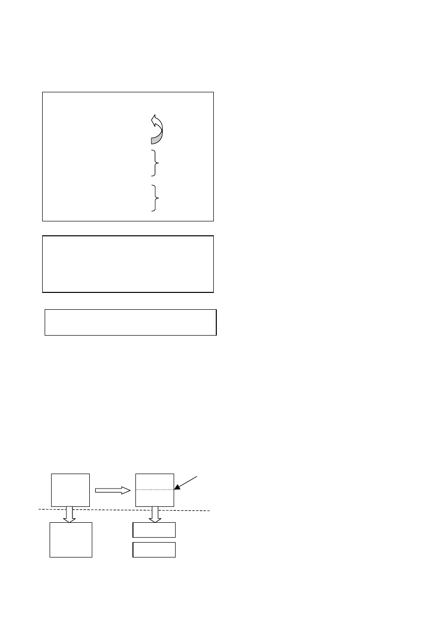
assembly we generated. We further omit the operands
and keep opcode, and we finally get abstract assembly
Figure 1.c.

One merit of dynamic instruction sequences over
assembly is that dynamic instruction sequences expose
some type of self-modifying behavior. If a program
modifies its code at runtime, we may observe two
different instructions at the same virtual address in
runtime trace. A program may modify its own code
more than once. We devise a mechanism to capture this
behavior while constructing logic assembly.

We associate an incarnation number with each virtual
address we have seen in the dynamic instruction
sequences. Initial incarnation number is 1. Each time we
met an instruction at the same virtual address, we
compare this assembly instruction with the one we have
seen before at that virtual address, if the instruction
changes, we increate the incarnation number.
Subsequent jump instruction will mark the beginning of
a basic block on the newest incarnation. We treat
instructions of different incarnation as different code
segment, and generate basic blocks separately. Figure 2
illustrate this process.

In this way we keep the behavior of any historical invo-
cations even the code is later overwrote by newly
generated code.

INSTRUCTION ASSOCIATIONS

Once we get abstract assembly, we are interested in
finding relationship among instructions within each
basic block. We believe the way instruction sequences
groups together within each block carries the
information of the behavior of an executable.

The instruction sequences we are interested in are not
limited to consecutive and ordered sequences. Virus
writers frequently change the order of instructions and
insert irrelevant instructions manually to create a new
virus variation. Further, metamorphism viruses [3]
make this process automatic. The resulting virus
variation still carries the malicious behavior. However,
any detection mechanism based on consecutive and
ordered sequences such as N-Gram could be fooled.

We have two considerations to obtain the relationship
among instructions. First, whether the order of
instructions matters or not; Second, whether the
instructions should be consecutive or not. Based on
these two criteria, we use three methods to collect
features.

1. The order of the sequences is not considered and

there could be instructions in between.

2.

The order of instructions is considered, however, it
is not necessary for instruction sequences to be
consecutive.

3.

The instructions are both ordered and consecutive.

We call these “Type 1”, “Type 2” and “Type 3”
instruction associations. “Type 3” instruction
association is similar to N-Gram. “Type 2” instruction
association can deal with garbage insertion. “Type 1”
instruction can deal with both garbage insertion and
code reorder.
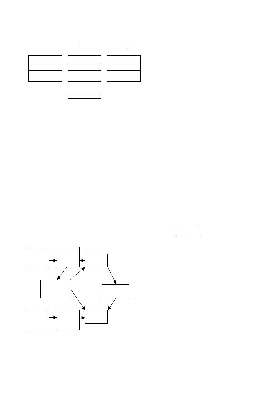
Figure 3 illustrates different type of instruction associa-
tions of length 2 we have obtained on an instruction se-
quence consisting of 4 instructions.

b. Logic Assembly

a. Original Log

01002157 loc1 pop

ecx

01002158

lea ecx,dword ptr ds:[eax+1]

0100215b loc2 mov dl,byte ptr ds:[eax]
0100215d

inc eax

0100215e

test dl,dl

01002160

jnz short 0100215b

1. 01002157 pop ecx
2. 01002158 lea ecx, ds:[eax+1]
3. 0100215b mov dl, ds:[eax]
4. 0100215d inc eax
5. 0100215e test dl,dl
6. 01002160 jnz short 0100215b
7. 0100215b mov dl, ds:[eax]
8. 0100215d inc eax
9. 0100215e test dl,dl
10.01002160 jnz short 0100215b
11.0100215b mov dl, ds:[eax]
12.0100215d inc eax
13.0100215e test dl,dl
14.01002160 jnz short 0100215b

Repetition

Repetition

loc1 pop

lea

loc2

mov inc test jnz

c. Abstract Assembly

Figure 1 Logic Assembly and Abstract Assembly

Modified to

jump to

Incarnation 1

Incarnation 2

generate logic assembly

basic block 1

basic block 2

basic block 3

Figure 2 Different Incarnations

DATA MINING PROCESS

The overall data mining process can be divided into 7
steps. They are:

1. Run executable inside a virtual machine, obtain in-

struction sequences from Ollydbg

2.

Construct logic assembly

3.

Generate abstract assembly

4. Select

instruction

associations features

5. Extract frequency of instruction associations

features in the training dataset and testing dataset

6.

Build classification models

7.

Apply classification models on testing dataset

This process is illustrated in figure 4.



















Here we describe step 4 in detail. The features for our
classifier are selected instruction associations. To select
appropriate features, we use the following two criteria:

1. The instruction associations should be not too rare

in the training dataset consisting of both benign
and malicious executables. If it occurs very rare,
we would rather consider this instruction
association is a noise and not use it as our feature

2. The instruction associations should be an indicator

of benign or malicious code; In other words, it
should be abundant in benign code and rare in
malicious code, or vice versa.

To satisfy the first criteria, we extract frequent instruc-
tion associations from training dataset. Only frequent
instruction associations can be considered as our feature.
We use a variation of Apriori algorithm [26] to generate
all three types of frequent instruction associations from
abstract assembly. Although there exists algorithms to
optimize Apriori algorithm [30], the optimization only
applicable to type 1 instruction association, besides, this
step only occurs at training time. We believe optimize
applying process is more critical because it will run on
each computer under protection. Training, however,
only need to be done on a specific hardware.

One parameter of Apriori algorithm is “minimum sup-
port”. It is the minimal frequency of frequent
associations among all transactions. More specifically,
it is the minimum percentage of basic blocks that
contains the instruction sequences in our case. We do
experiments on different support level as described in
out experimental result.

To satisfy the second criteria, we define the term

contrast

CountB (F

i

) normalized count of F

i

in benign

instruction file

CountM (F

i

) normalized count of F

i

in malicious

instruction file

ε

a small constant to avoid error when the
dominant is 0

In this formula definition, normalized count is the fre-
quency of that instruction sequence divided by the total
number of basic blocks in abstract assembly. We use a
larger benign code dataset than malicious code dataset.
The use of normalization will factor out the effect of
unequal dataset size.

We select top L features as our feature set. For one ex-
ecutable in training dataset, we count the number of
basic blocks containing the feature, normalized by the
number of basic blocks of that executable. We process
every executable in our training dataset, and eventually
we generate the input for our classifier.

Type 1

push sub

mov sub

mov push

Type 2

sub push

sub mov

sub sub

push mov

push sub

mov sub

Type 3

sub push

push mov

mov sub

Instruction Sequences:

Figure 3 Instruction Associations of Length 2

sub push mov sub

⎪

⎪

⎩

⎪⎪

⎨

⎧

<

+

+

≥

+

+

=

)

(

)

(

)

(

)

(

)

(

)

(

)

(

)

(

)

(

Fi

countM

Fi

countB

Fi

countB

Fi

countM

Fi

countM

Fi

countB

Fi

countM

Fi

countB

Fi

Contrast

ε

ε

ε

ε

Figure 4 Data Mining Process

Training

Instruction

Sequences

Training

Abstract

Assembly

Top Instruction

Association

Features

Training

Dataset

Testing

Instruction

Sequences

Testing

Abstract

Assembly

Testing
Dataset

Classification

Model

Build

Apply

We use two classifiers in our experiment: C4.5 decision
tree [27] and libSVM [28] Support Vector Machine.

C4.5 decision tree is a classification algorithm that is
constructed by recursively splitting the dataset into parts.
Each such split is determined by the result of the
entropy gain of all possible splits among all attributes
inside the tree node. The decision tree keeps growing as
more splits are performed until a specific stop rule is
satisfied. During postpruning, some splits are removed
to relieve overfitting problem. When a record of an
unknown class comes in, it is classified through a
sequence of nodes from the tree root down to the leaf
node. Then, it is labeled by the class the leaf node
represents.

Support Vector Machine (SVM) [35] is essentially a
ma-thematical optimization problem which is originated
from the linear discriminant problem. However, if two
classes are inseparable in two dimensions, SVM can use
a mapping, which is called kernel function, to map two
dimension data into a higher dimension. The two
classes may be separable in higher dimension. libSVM
is a popular C implementation of SVM on Unix.

We also tested some other classifiers such as random
forest [33]. We do not detect any classifier has clear
advantage over others in the measure of accuracy.
However, one reason drives us to use C4.5 and SVM in
our experiment is that both classifiers are efficient to
make decision. The performance of decision making
process is the key to the system performance (See
performance analysis).

EXPERIMENTAL RESULTS

Dataset
Due to the prevailing dominance of Win32 viruses to-
day, we only use Win32 viruses as our virus dataset.
We collect 267 Win32 viruses from VX heaven [17].

We also choose 368 benign executables which consist
of Windows system executables, commercial
executables and open source executables. These
executables have the similar average size and variation
as the malicious dataset.

For both malicious and benign codes, we randomly
choose 70% of them as a training dataset and the
remain-ing 30% as a testing dataset.

Criteria
In out experiment, we use accuracy on testing dataset as
our main criteria to evaluation the performance of
classification models. However, we also calculate false
positive rate and false negative rate. False positive rate
is the proportion of benign executables that were
erroneously reported as being malicious. On contrary,
false negative rate is the proportion of malicious

executables that were erroneously identified as benign.
We believe in a virus detection mechanism, low false
negative rate is more vital than low false positive rate. It
is wise to be more cautious against those suspicious un-
known executables. High false positive certainly make
things inconvenient for the user, but high false negative
will destroy user’s computer, which is more harmful.

Parameter Selection
There are five primary parameters in our classifier, they
are:
1.

Instruction association type IA (type 1, 2 or 3)

2. Support level of frequent instruction association

(S). We experiment 0.003, 0.005, 0.01

3. Number of features (L), we try 10, 20, 50, 100,

200, 300. At some support level, some instruction
association type generates relatively fewer number
of available features. For example, at support lever
0.01, only 23 type 1 instruction associations are
frequent. In that case, we use up to the maximum
available features

4. Type of classifier (C), we compare C4.5 decision

tree and SVM (Support Vector Machine)

5. Number of instruction captured (N). We try 1000,

2000, 4000, 6000, 8000

IA S L C N Accuracy

2 0.01 300 SVM 1000 0.962/0.930
1 0.01 200 C45 1000 0.919/0.923
1 0.01 200 C45 6000 0.943/0.923
2 0.01 300 SVM 8000 0.950/0.920
1 0.01 200 SVM 2000 0.924/0.919
2 0.01 200 C45 8000 0.960/0.918
1 0.01 300 C45 8000 0.945/0.918
1 0.01 200 C45 8000 0.941/0.918
1 0.01 300 C45 4000 0.919/0.918
2 0.01 300 SVM 4000 0.955/0.914

Table 1 Top 10 Configurations

Table 1 lists top 10 configurations we get along with
accuracy on both training dataset and testing dataset.

The result shows that support level 0.01 is clearly
superior to others. It shows that frequent patterns are
more important than infrequent patterns.

Instruction association type 1 and 2 outperform type 3.
That is an interesting result which could serve to justify
our approach in that traditional N-Gram based approach
checks type 3 instruction association only.

The effect of number of instructions captured N is not
quite clear yet. We further calculate average accuracy at
different n in figure 5. We see that in general accuracy

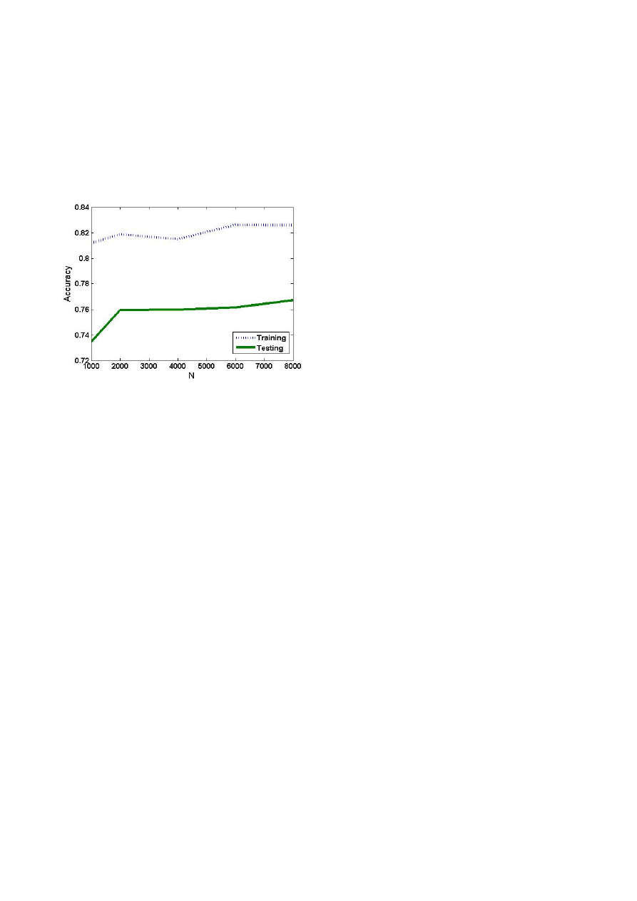
increase when we use a large N. However, the
difference becomes very small when N>2000. That
justify that when we use the first 4000 instructions, we
can capture the behavior of the unknown executable.
One interesting phenomenon is when N=1000, we get
some really good result. Our top 2 classifiers all have
the setting N=1000. That means in some settings, first
1000 instructions already capture the character of the
executable, further instructions might only give noises.

Figure 5 Effect of N

Model Selection
One problem in our best performed classifier is that it
uses 300 features. The number of features affects the
per-formance of our detector (See performance
analysis). To this end, we choose the second best setting.
The false positive rate for this classifier is 0.114, and
the false negative rate is 0.013. We don’t have space to
show more data for false positive rate and false negative
rate. In general, false positive rate is much higher than
false negative rate in our experiments. That is exciting
because we expect a lower false negative rate.

PERFORMANCE ANALYSIS

In this section, we focus on performance when applying
the classification model on the end user computer. The
performance to process one unknown executable is
determined by the following factors: Capturing
instruction sequences; Generating logic assembly;
Counting the occurrence of instruction associations in
feature set to generate testing features; Applying
classification model.

Unlike system call, instruction sequences generate fast
and at a stable rate. On our test computer, we generate
around 6,000 instruction sequences in 1 second under
Ollydbg. That is enough for the input for our classifier.
This is the one major advantage over system call
approach, which takes time to get enough system call
traces.

Generating logic assembly consists of three phases. In
the first phase, we need to sort the instruction sequences
according to their virtual address. This could take up to

O(nlogn) to finish. In the second phase, we mark jump
destination using one linear scan of all instructions,
which takes O(n). Maintaining different incarnations
requires a memory map to remember the instruction and
incarnation of each virtual address. Every instruction
takes linear time to check this memory map, so this
additional task will not increase the order of the overall
processing time. Finally, we traverse the sorted
instruction list to output basic blocks, which takes O(n).
So the overall time complexity in logic assembly
generation is O(nlogn).

Generating testing features requires counting the fre-
quency of L features. Suppose average basic block
contains k instructions, thus we have average n/k basic
blocks. For every basic block, we will do a search for
each one of L features.

Different types of instruction association use different
approach to search inside a basic block. For type 1
instruction association, we use an occurrence bit for
every instruction in the association, if all bit is on, then
the basic block contains that instruction association. For
type 2, we construct a finite state machine (FSM), and
scan the basic block from the beginning. If we
encounter an instruction matching the state in FSM, we
advance the state of FSM, and begin matching the next
instruction. For type 3, it is similar to a substring search.
All these three types of search requires only one linear
scan of the basic block, makes the bound of O(k).

We can calculate the processing time of testing feature
generation as the multiply of the above factors. So this
step takes (search time per feature per block)* (feature
number) * (basic block number) = O(n/k*k*L) = O(nL).

The time complexity to apply a classification model is a
property of specific classification model. For C4.5
decision tree, the applying time complexity is
proportional to the depth of the tree [27], which is a
con-stant at the applying time. SVM takes O(L) to apply
the model on a specific sample [31].

Based on the discussion above, we conclude that the
time complexity to process an unknown executable is
bounded by max (O(nlogn), O(nL)), in which n is the
number of instructions captured, L is the number of
features.

In our experiment, processing instructions captured in 1
second, for which n ≈ 6000, the calculation time is
usually less than 3 seconds. This suggests that this
approach can be used in practice.

CONCLUSION

In this paper, we have proposed a novel malicious code
detection approach by mining dynamic instruction
sequences and described experiments conducted against
recent Win32 viruses.

Experimental results indicate that the proposed data
mining approaches can detect malicious codes reliably
even for the unknown computer viruses. The best
classification rate on testing dataset is 93.0%. The
performance in measure of time is acceptable in
practical usage.

Compared with other approaches, instruction associa-
tion deal with the virus code directly and is robust to
me-tamorphism.

We also plan to build an end user simulator based on
the best data mining model. The simulator will run the
unknown executable inside a controlled environment,
capture initial dynamic instruction sequences and make
decision based on them.

REFERENCES

[1] Microsoft Antimalware Team , “Microsoft Security Intelligence

Report”, Volume 3, 2007,
http://www.microsoft.com/security/portal/sir.aspx

[2] C. Nachenberg, “Computer virus-antivirus coevolution”,

Communications of the ACM, Volume 40 , Issue 1, pp:46–51, 1997

[3] P. Sz¨or and P. Ferrie, “Hunting for metamorphic”, 11

th

International Virus Bulletin Conference, Prague, Czech Republic,
2001

[4] Jeffrey O. Kephart, William C. Arnold, "Automatic Extraction of

Computer Virus Signatures", 4

th

International Virus Bulletin

Conference, Jersey, Channel Islands, 1994.

[5] Stuart Staniford, Vern Paxson, Nicholas Weaver, "How to 0wn the

Internet in Your Spare Time", 11

th

Usenix Security Symposium,

San Francisco, USA, 2002

[6] F. Cohen, “Computational Aspects of Computer Viruses”,

Computers & Security, volume 8, pp:325-344, 1989

[7] William Arnold, Gerald Tesauro, "Automatically generated Win32

heuristic virus detection", 10

th

International Virus Bulletin

conference, Orlando, FL, USA, 2000

[8] InSeon Yoo, "Visualizing windows executable viruses using self-

organizing maps", Proceedings of the 2004 ACM workshop on
Visualization and data mining for computer security, Fairfax, VA,
USA, 2004

[9] Matthew G. Schultz, Eleazar Eskin, Erez Zadok, and Salvatore J.

Stolfo, "Data Mining Methods for Detection of New Malicious
Executables", Proceedings of IEEE Symposium on Security and
Privacy, Oakland, CA, USA, 2001

[10] Abou-Assaleh, Nick Cercone, Vlado Keselj, and Ray Sweidan,

"Detection of New Malicious Code Using N-grams Signatures",
Proceedings of the Second Annual Conference on Privacy,
Security and Trust (PST'04), pp: 193-196, Fredericton, New
Brunswick, Canada, 2004

[11] Abou-Assaleh, Nick Cercone, Vlado Keselj, and Ray Sweidan, “N-

Gram-based Detection of New Malicious Code”, Proceeding of the
28th Annual International Computer Software and Applications
Conference (COMPSAC’04), Hong Kong, China, 2004

[12] Kolter, J.Z., & Maloof, M.A., "Learning to detect malicious

executables in the wild", In Proceedings of the 10

th

ACM SIGKDD

International Conference on Knowledge Discovery and Data
Mining, pp:470-478. New York, NY, 2004.

[13] Sung, A.H et al “Static analyzer of vicious executables (SAVE)”,

20

th

Annual Computer Security Applications Conference, Tucson,

AZ, USA, 2004

[14] Mihai Christodorescu, Somesh Jha, Sanjit A. Seshia, Dawn Song,

Randal E. Bryant, "Semantics-Aware Malware Detection", IEEE
Symposium on Security and Privacy, Oakland, CA, USA, 2005

[15] Mihai Christodorescu, Somesh Jha, "Static Analysis of Executables

to Detect Malicious Patterns", 12

th

USENIX Security Symposium,

Washington DC, USA, 2003

[16] Christopher Kruegel et al, “Static Disassembly of Obfuscated

Binaries”, Proceedings of the 13

th

conference on USENIX Security

Symposium, San Diego, CA, USA, 2004

[17] Cullen Linn et al, “Obfuscation of Executable Code to Improve

Resistance to Static Disassembly”, Proceedings of the 10

th

ACM

conference on Computer and communications security,
Washington D.C., USA, 2003

[18] B. Schwarz, S. Debray, G. Andrews, "Disassembly of Executable

Code Revisited," wcre, p. 0045, 9

th

Working Conference on

Reverse Engineering, Richmond, Virginia, USA, 2002

[19] Bayer, U., Kruegel, C., Kirda, E, “TTAnalyze: A Tool for Analyzing

Malware”, 15

th

Annual Conference of the European Institute for

Computer Antivirus Research, Hamburg, Germany, 2006

[20] Steven A. Hofmeyr et al, ”Intrusion detection using sequences of

system calls”, Journal of Computer Security, Volume 6 , Issue 3,
pp

:

151-180, 1998

[21] Wenke Lee and Salvatore J. Stolfo, “Data Mining Approaches for

Intrusion Detection”, 7

th

USENIX Security Symposium, San

Antonio, Texas, USA, 1998

[22] Warrender, C et al, “Detecting intrusions using system calls:

alternative data models”, Proceedings of the IEEE Symposium on
Security and Privacy, Oakland, CA, USA, 1999

[23] Tony Lee, Jigar J. Mody, “Behavior Classification”, 2006,

http://blogs.technet.com/antimalware/archive/2006/05/16/42
8749.aspx

[24] http://www.ollydbg.de/
[25] Md. Enamul. Karim et al, “Malware Phylogeny Generation using

Permutations of Code”, Journal in Computer Virology, Volume 1,
Numbers 1-2, 2005

[26] Rakesh Agrawal, Ramakrishnan Srikant, "Fast Algorithms for

Mining Association Rules", Proc. 20

th

International Conference of

Very Large Data Bases, VLDB, Santiago de Chile, Chile, 1994

[27] J.R.Quinlan, “C4.5:Programs for Machine Learning”, Morgan

Kaufmann Publishers Inc, 1993

[28] http://www.csie.ntu.edu.tw/~cjlin/libsvm/
[29] http://vx.netlux.org
[30] Jiawei Han , Jian Pei , Yiwen Yin, “Mining frequent patterns

without candidate generation”, Proceedings of the ACM
SIGMOD international conference on Management of data, Dallas,
Texas, USA, 2000

[31] Vladimir Vapnik, “Statistical Learning Theory”, John Wiley &

Sons, 1998

[32] http://research.microsoft.com/sn/detours/
[33] Breiman L, "Random Forests", Machine Learning Volume 45, pp:5-

32, Kluwer Academic Publishers, 2001

[34] http://www.isotf.org/zert/
[35] John Shawe-Taylor & Nello Cristianini, "Support Vector

Machines", Cambridge University Press, 2000