Collaborative Defense Against Zero Day and Polymorphic Worms Detection, Response and an Evaluation Framework

Collaborative Defense Against Zero-Day and Polymorphic Worms:

Detection, Response and an Evaluation Framework

SENTHILKUMAR G CHEETANCHERI

B.E. (Coimbatore Institute of Technology, India) 1998

M.S. (University of California, Davis) 2004

DISSERTATION

Submitted in partial satisfaction of the requirements for the degree of

DOCTOR OF PHILOSOPHY

Computer Science

in the

OFFICE OF GRADUATE STUDIES

of the

UNIVERSITY OF CALIFORNIA

DAVIS

Approved:

Professor Karl N. Levitt(Chair)

Professor Matthew Bishop

Associate Professor Felix Wu

Doctor John-Mark Agosta

Committee in Charge

2007

–i–

Collaborative Defense Against Zero-Day and Polymorphic Worms:

Detection, Response and an Evaluation Framework

Senthilkumar G Cheetancheri

To my Parents

iii

Contents

Acknowledgements

vii

Abstract

viii

Introduction

1.1

Contributions . . . . . . . . . . . . . . . . . . . . . . . . . . . . . . . . . . .

An overview of Worm Research

2.1

An overview of worms . . . . . . . . . . . . . . . . . . . . . . . . . . . . . .

2.1.1

Hello Worm! . . . . . . . . . . . . . . . . . . . . . . . . . . . . . . .

2.1.2

Worm Examples . . . . . . . . . . . . . . . . . . . . . . . . . . . . .

2.1.3

Scanning algorithms . . . . . . . . . . . . . . . . . . . . . . . . . . .

2.1.4

Scanning Constraints . . . . . . . . . . . . . . . . . . . . . . . . . . .

2.2

Problems, Paradigms & Perspectives . . . . . . . . . . . . . . . . . . . . . .

2.3

Modeling of worms . . . . . . . . . . . . . . . . . . . . . . . . . . . . . . . .

2.4

Prevention . . . . . . . . . . . . . . . . . . . . . . . . . . . . . . . . . . . . .

2.4.1

Prevention of vulnerabilities . . . . . . . . . . . . . . . . . . . . . . .

2.4.2

Prevention of exploits . . . . . . . . . . . . . . . . . . . . . . . . . .

2.4.3

The Diversity Paradigm . . . . . . . . . . . . . . . . . . . . . . . . .

2.5

Detection Systems . . . . . . . . . . . . . . . . . . . . . . . . . . . . . . . .

2.5.1

Network Traffic Analysis . . . . . . . . . . . . . . . . . . . . . . . . .

2.5.2

Run-time Program analysis . . . . . . . . . . . . . . . . . . . . . . .

2.6

Response Systems . . . . . . . . . . . . . . . . . . . . . . . . . . . . . . . .

2.6.1

Response Selection . . . . . . . . . . . . . . . . . . . . . . . . . . . .

2.7

Evaluation Systems . . . . . . . . . . . . . . . . . . . . . . . . . . . . . . . .

2.7.1

Simulations . . . . . . . . . . . . . . . . . . . . . . . . . . . . . . . .

2.7.2

Emulation on Testbeds . . . . . . . . . . . . . . . . . . . . . . . . . .

Evaluation Framework

3.1

Introduction . . . . . . . . . . . . . . . . . . . . . . . . . . . . . . . . . . . .

3.2

Motivation

. . . . . . . . . . . . . . . . . . . . . . . . . . . . . . . . . . . .

3.3

The Framework . . . . . . . . . . . . . . . . . . . . . . . . . . . . . . . . . .

3.3.1

NS to NS-testbed compiler . . . . . . . . . . . . . . . . . . . . . . .

3.3.2

Pseudo Vulnerable Servers . . . . . . . . . . . . . . . . . . . . . . . .

3.3.3

The worm library . . . . . . . . . . . . . . . . . . . . . . . . . . . . .

3.3.4

The Event Control System . . . . . . . . . . . . . . . . . . . . . . .

3.3.5

Data Analysis Tools . . . . . . . . . . . . . . . . . . . . . . . . . . .

3.4

The API . . . . . . . . . . . . . . . . . . . . . . . . . . . . . . . . . . . . . .

3.4.1

User Inputs . . . . . . . . . . . . . . . . . . . . . . . . . . . . . . . .

3.5

An Example - The Hierarchical Model of worm defense . . . . . . . . . . . .

3.5.1

Modeling the system . . . . . . . . . . . . . . . . . . . . . . . . . . .

3.5.2

The experiment . . . . . . . . . . . . . . . . . . . . . . . . . . . . . .

3.5.3

Results . . . . . . . . . . . . . . . . . . . . . . . . . . . . . . . . . .

3.6

Future work . . . . . . . . . . . . . . . . . . . . . . . . . . . . . . . . . . . .

A Distributed Worm Detection System

4.1

Introduction . . . . . . . . . . . . . . . . . . . . . . . . . . . . . . . . . . . .

4.2

A Distributed Collaborative Defense . . . . . . . . . . . . . . . . . . . . . .

4.2.1

Collaborative Distributed Attack Detection . . . . . . . . . . . . . .

4.2.2

Cooperative Messaging Protocols . . . . . . . . . . . . . . . . . . . .

4.3

Evaluation on an Emulated Test-bed . . . . . . . . . . . . . . . . . . . . . .

4.3.1

Experimental Setup . . . . . . . . . . . . . . . . . . . . . . . . . . .

4.4

Experimental Results . . . . . . . . . . . . . . . . . . . . . . . . . . . . . . .

4.4.1

False Alarm Experiments . . . . . . . . . . . . . . . . . . . . . . . .

4.4.2

Performance in Detecting Worm Attacks . . . . . . . . . . . . . . . .

4.5

Future Work . . . . . . . . . . . . . . . . . . . . . . . . . . . . . . . . . . .

Response using Dynamic Programming

5.1

Introduction . . . . . . . . . . . . . . . . . . . . . . . . . . . . . . . . . . . .

5.2

Dynamic Programming

. . . . . . . . . . . . . . . . . . . . . . . . . . . . .

5.3

DP Problems with imperfect state information . . . . . . . . . . . . . . . .

5.3.1

Problem Description . . . . . . . . . . . . . . . . . . . . . . . . . . .

5.3.2

Re-formulation as a Perfect State-information Problem . . . . . . . .

5.4

Response Formulation with imperfect State information . . . . . . . . . . .

5.4.1

Problem Statement . . . . . . . . . . . . . . . . . . . . . . . . . . . .

5.4.2

Problem Formulation

. . . . . . . . . . . . . . . . . . . . . . . . . .

5.4.3

Solution . . . . . . . . . . . . . . . . . . . . . . . . . . . . . . . . . .

5.5

Alternate Re-formulation using Sufficient Statistics . . . . . . . . . . . . . .

5.5.1

Sufficient Statistic . . . . . . . . . . . . . . . . . . . . . . . . . . . .

5.5.2

Conditional State Distribution . . . . . . . . . . . . . . . . . . . . .

5.5.3

Reduction using Sufficient Statistics . . . . . . . . . . . . . . . . . .

5.5.4

Response Formulation using Sufficient Statistics

. . . . . . . . . . .

5.6

A Practical Application . . . . . . . . . . . . . . . . . . . . . . . . . . . . .

5.6.1

Optimal Policy . . . . . . . . . . . . . . . . . . . . . . . . . . . . . .

5.6.2

Choosing λ . . . . . . . . . . . . . . . . . . . . . . . . . . . . . . . .

5.6.3

Larger N s . . . . . . . . . . . . . . . . . . . . . . . . . . . . . . . . .

5.7

Evaluation . . . . . . . . . . . . . . . . . . . . . . . . . . . . . . . . . . . . .

5.7.1

Experiments . . . . . . . . . . . . . . . . . . . . . . . . . . . . . . .

5.7.2

Effects of increasing N . . . . . . . . . . . . . . . . . . . . . . . . . .

5.8

Limitations and Future Work . . . . . . . . . . . . . . . . . . . . . . . . . .

Conclusion

6.1

Summary . . . . . . . . . . . . . . . . . . . . . . . . . . . . . . . . . . . . .

6.2

Future Directions . . . . . . . . . . . . . . . . . . . . . . . . . . . . . . . . .

6.3

Final Observations . . . . . . . . . . . . . . . . . . . . . . . . . . . . . . . .

Bibliography

Acknowledgements

I would first like to thank my mentor Jeff Rowe without whom I would not be

writing this dissertation. He has been an eternal source of ideas and practical advice

through out the course of my doctoral research. A person of great kindness who tolerated

all my follies and continued to teach and guide me. Next, I would like to thank my advisor

Karl Levitt who has been more than a research advisor to me. He has been a great friend

who stood by me through thick and thin the past six years at school as well as in my

personal life – a wedding, a child birth and three funerals. I’m yet to meet a kinder person

than these two.

I would always cherish the inspiring discussions I had with John-Mark Agosta at

Intel. I thank him a lot for reading the numerous drafts of ideas, papers and this dissertation

with a fine comb and providing his insightful and thought-provoking comments over the past

three years. I thank Felix Wu and Todd Heberlein for those numerous inspirational chats

and putting graduate school in perspective. I thank Matt Bishop for reading drafts of this

dissertation and providing timely feedback.

Life would have been much harder without my dear friends at the Security Lab,

Ebrima Ceesay, Denys Ma, Lynn Nguyen, Marcus Tylutki, Tufan Demir and Allen Ting

who formed a great group to share all the fun and frustrations of graduate school. I have to

thank the American education system and UCDavis for providing me this great educational

and cultural immersion that I never imagined possible before coming to Davis.

Finally, I thank my family – partiularly my father who weathered the numerous

misfortunes single-handedly all the way across the seven seas and let me carry on with my

graduate school.

vii

Abstract

Computer worms present a grave concern to the common man, and a challenging

problem to the computer security community. Worms’ abilities have precluded human in-

tervention. Fast worms can be too fast to respond to. Slow worms can be too slow to be

noticed. Zero-day and polymorphic worms can look like ordinary traffic to evoke any sus-

picion until they cause large scale destruction. This demands not just automated response

but automated and intelligent response. This dissertation presents such an automated and

intelligent means of detecting and responding to zero-day worms that could possibly be

polymorphic in a signature independent fashion.

Worms are detected cooperatively using a novel distributed application of the long-

established Sequential Hypothesis Testing technique. The technique developed here builds

a distributed worm detector of any desirable fidelity from unreliable anomaly detection

systems. Tracking anomalies instead of signatures enables detection of zero-day and poly-

morphic worms. Cost-effective responses in the face of uncertainty about worms are selected

automatically using Dynamic Programming. Responses are selected based on the likelihood

of a current worm attack, and the relative costs of infection and responses, while minimizing

the operating cost over a period of time. This technique uses information about anomalous

events, potentially due to a worm, observed by cooperating peers to choose optimal actions

for local implementation.

In addition to developing the above techniques, this dissertation also presents a

generic testing framework based on the Emulab network testbed to evaluate these and other

such worm defense models, and provides a detailed survey of the research done so far in

worm defense.

viii

CHAPTER 1.

INTRODUCTION

Chapter 1

Introduction

Computer worms are a serious problem. Over the decades, it has transformed

from being an useful tool for distributed computing to a lethal tool chest of cyber criminals

and one of the worst nightmares for legitimate computer users. Worms could be used by

attackers and terrorists to launch various kinds of attacks such as denial-of-service, massive

identity theft, and to scout for unguarded computers that can be subscribed to botnets.

These can later be used for nefarious activities such as spam campaigns, phishing attacks,

and illicit international financial transactions among others.

Tremendous progress has been made in the past decade to deal with worms. Worms

manifest themselves through some of their activities which are anomalous with the usual

operations or through damages they cause. They are then captured, analyzed manually and

appropriate techniques are engineered and deployed to mitigate their ill-effects. However,

given the speed with which they can spread, such manual analysis is too slow and the battle

is lost even before it is fought. Worms can also spread so slow that any ill-effects they cause

seem as isolated incidents rather than correlated events. Worms could also be programmed

not to reveal themselves until all susceptible computers are infected, and then unleash their

lethal force all at once at a pre-determined time or upon receipt of a commands. Such

dangerous potentials of worms render manual intervention ineffective and warrant a timely

and automatic detection of, and response to, worms.

One technique that has wide-spread prevalence and exemplary commercial success

is traffic filtering based on signatures of worms. A signature is any string in the body of the

worm that is unique to it; unique in the sense, that there is no other known worm with the

same string. This method exploits the fact that a worm is after all a sequence of bits, and

CHAPTER 1.

INTRODUCTION

a regular expression can be developed for a pattern unique to each worm. All traffic that

enters a network or a machine, or crosses any boundary of interest, is compared against

this regular expression. If there is a match, the given response action is taken. A typical

response would be to drop the connection and inform the responsible authority about the

incident. If there are multiple worms to be guarded against, multiple regular expressions are

used. Sophisticated algorithms, including proposals to incorporate them in hardware, are

used to perform this pattern matching at high speeds to keep up with the ever-increasing

performance of network devices delivering more volume of traffic in lesser time.

This technique naturally does not work against unknown worms and polymorphic

worms. Unknown worms also known as Zero-day worms use novel attacks or exploit hitherto

unknown vulnerabilities. Polymorphic worms, on the other hand, change their appearance

while preserving the semantics each time they spread from one victim to another. Tech-

niques such as encryption and instruction re-ordering are used to achieve this polymorphism

making their identification with pattern matching or signature matching ineffective even if

the worm’s details and mode of operation are known. Together, zero-day worms and poly-

morphic worms present a great challenge for computer and network administrators as well

as researchers. Despite huge strides during the past few years, dealing with these two are

still active research topics.

Once an outbreak of a worm has been detected, responding to it becomes trivial –

shutdown services until a suitable solution is worked out . There is no point in continuing

service without adequate safety guards when it is clear that infection is imminent. Suitable

solutions could be automatic or manual distribution and installation of patches, signatures

or both, or any other such strategies. However, one cannot really wait until a worm is

authoritatively detected. There is a need to take evasive actions even while the detection

process is in progress. Shutting down the service completely is definitely one such candidate

response. Alternatively, a reduced service can be provided by scrutinizing every service

request for infection attempts by a worm. Choosing whether or not to take evasive actions

becomes challenging as the costs of such actions in response to false alarms must be balanced

against the costs of infection.

The novel ideas for detecting zero-day worms explored in this dissertation deal

with these two kinds of worms from a signature-independent perspective. This dissertation

develops methods to detect worms in a distributed and collaborative fashion by exchanging

and corroborating reports about anomalous events. Current anomaly detectors are prone

CHAPTER 1.

INTRODUCTION

to high false positives. The methods developed here use a distributed version of a statistical

tool called Sequential Hypothesis Testing [113] to build a strong distributed worm detector

from imperfect or weak anomaly detectors as the building blocks. Chapter 3 details the

algorithm and the protocols used to detect zero-day worms.

This dissertation also develops a control-theoretic approach for optimal cost re-

sponse to events that are possibly due to a worm. This approach uses dynamic-programming

techniques to generate a table of rules that can be looked-up during operation to determine

the optimal-cost action to take in response to possible worm-events. The details of this idea

is developed in chapter 4.

Apart from these two techniques, chapter 2 develops an evaluation framework that

makes it easy to test these and other such new methodologies on an isolated network testbed

such as Emulab or DETER. The next chapter, presents a overview, and a brief history of

worms and an overview the latest technologies that are being developed and used in the

worm research field.

1.1

Contributions

This dissertation makes several contributions to the field of worm research.

• First and foremost it develops holistic solutions to the worm problem, detection as

well as response, from a content-independent perspective and making use of anomaly

detection. This is a paradigm shift from the current solutions that look for certain

patterns in the worm content called signatures. This is a major contribution as it

is very difficult, if not impossible, to generate and detect new high speed worms or

polymorphic worms with signature-specific approaches.

• An important contribution of this dissertation is that it moves away from a centralized

control element that is a requirement in most of the other systems proposed so far

and thus providing fault-tolerance to the system.

• This dissertation builds an evaluation framework which can be used to quickly and

easily deploy and test new worm defense systems. This framework consists of the

necessary software infrastructure to conduct experiments in the EMULAB [120] and

DETER [16] network testbeds to evaluate new algorithms against worms.

CHAPTER 1.

INTRODUCTION

• A high fidelity distributed worm detector is developed in this dissertation using im-

perfect and unreliable components such as anomaly detectors that have high false

positive rates. This has been achieved using a novel distributed application of a

statistical technique called Sequential Hypothesis Testing(dSHT) .

• This dissertation develops a control-theoretic approach to response, independent of

any particular worm. The response mechanism is designed to make use of the dSHT

developed here to detect the worm and apply Dynamic Programming techniques to

choose the appropriate response from a give set of responses.

CHAPTER 2.

AN OVERVIEW OF WORM RESEARCH

Chapter 2

An overview of Worm Research

There is a vast literature detailing the history, evolution and mechanics of worms

[33]. In this chapter, we will present a quick overview of these aspects first in Sec. 2.1, and

devote the rest of the chapter to present more detailed discussions on the current paradigms

that govern the state-of-the-art in prevention, detection, and response and mitigation tech-

niques against worms.

The problem of worms can be partitioned into several sub-problems and each

one is currently being addressed from several perspectives using a variety of tools from

mathematics to machine learning to software engineering. Sec. 2.2 of this chapter presents

this overview of the problem space. The two sections following that delve deeper into the

work done so far by the research community to address two of the sub-problems, viz-a-viz,

detection and mitigation. The last section talks about evaluation systems that can evaluate

these research efforts – including new worms, detection and response. This chapter also sets

up the stage for the rest of this dissertation by identifying the gaps in the current research.

2.1

An overview of worms

This section provides a very basic understanding of a worm for the uninitiated and

then puts that in perspective by providing a few examples of old as well as hypothetical

worms. It also gives an overview of the various algorithms that can be used by worms to

look for new victims.

CHAPTER 2.

AN OVERVIEW OF WORM RESEARCH

2.1.1

Hello Worm!

A computer worm is an extremely handy tool to perform a particular task in a

distributed fashion or repetitively on several machines. Unfortunately, it can also be used

as a weapon. For example, consider a computing task that takes several days to perform

on a single machine. It can be done much quicker if it can be broken down to several

smaller and simpler sub-tasks that can be done in parallel on several machines. A parallel

processing machine will be very useful for this purpose. However, such a machine is usually

very complex, expensive and not very versatile. Instead of designing such a complex parallel

processing machine, we can design a comparatively simple tool that can assign sub-tasks to

capable idle machines and collect and compile the results. Such a tool is a worm.

When used properly a worm tries to hop on from one idle host to another carrying

with it a sub-task in search of computing power to accomplish its tasks and return the

results to the parent process that waits for the results on a different machine. A classic

example is the worm program that Shoch and Hupp used at the Parc to make use of idle

computing power of computers of several employees after regular office hours [97].

The most important requirement for a worm to perform a sub-task on a idle ma-

chine is, obviously, permissions to execute programs on it. In cases where prior permissions

are granted on various machines, the task is simple. In cases where permissions are not

granted the worm may try to force his or her way into other peoples’ computers. This can

be done by remotely exploiting one of the vulnerabilities that exist in those computers.

When a worm does this, it transforms from being an useful tool into a malicious software

(malware). When there is a particular vulnerability on many hundreds of machines spread

across the Internet, the Internet becomes a happy hunting ground for anyone that can

exploit that it. In fact, a vulnerability gives certain capabilities called primitives to the at-

tacker. For example, improper bounds checking in an array operation or an input operation

is a vulnerability that can give an attacker the ability to overwrite the return pointer on

the stack – also called smashing the stack [87]. The attacker can then use this primitive to

write several exploits.

2.1.2

Worm Examples

Morris Worm:

This was the first popular worm(released 1988). This worm located vul-

nerable hosts and accounts, exploited security holes on them to transfer a copy of the worm

CHAPTER 2.

AN OVERVIEW OF WORM RESEARCH

and finally ran the worm code. The worm obtained further candidate host IP addresses to

infect by examining the current victim’s /etc/hosts.equiv and /.rhosts files, user files like

.forward and .rhosts, dynamic routing information produced by the netstat program and by

randomly generating host addresses on local networks. It penetrated remote systems by ex-

ploiting the vulnerabilities in either the finger daemon, sendmail, or by guessing passwords

of accounts and using the rexec and rsh services to penetrate hosts that shared the same

account [50, 95, 101].

Code Red:

On June 18th 2001 a Windows IIS vulnerability was discovered. After about a

month a worm called Code-Red that exploited this vulnerability was released. It was buggy

and did not spread much. About a week after that, a truly virulent version was released.

This worm worked as follows. On each machine the worm generated 100 threads. Each of

the first 99 threads randomly chose an IP address and tried to set up a http connection

with it. If the connection was successful, the worm would send a copy of itself to the victim

to compromise it and continue to find another one. If the http connection could not be

set-up within 21 seconds, another random IP address was generated and the entire process

repeated. The worm’s payload was programmed to launch a denial-of-service attack against

the White House web-site at a pre-determined time. However, once the worm was detected

the attack was thwarted by the White House system administrators by moving the target

web-site to a different IP address [8, 32, 77, 124].

Slammer:

The Slammer worm [82], also known as the Sapphire Worm was the fastest

computer worm in history. It began spreading throughout the Internet at about 5:30 UTC,

on January 25 2003, and doubled in spread every 8.5 seconds. It infected more than 90

percent of vulnerable hosts within 10 minutes. Although very high speed worms [105] were

theoretically predicted about a year before the arrival of Slammer, it was the first live worm

that came any closer to such predicted speeds.

Slammer exploited a buffer overflow vulnerability in computers on the Internet

running Microsoft’s SQL Server or MSDE 2000. This vulnerability in an underlying indexing

service was discovered in July 2002. Microsoft released a patch for the vulnerability before

it was announced but many system administrators around the world didn’t apply the patch

for various reasons. The following were some of the reasons. The patch was more difficult

to install than the original software itself. They were afraid that applying the patch might

CHAPTER 2.

AN OVERVIEW OF WORM RESEARCH

disturb their current server settings while it was always not trivial to tune a software to

the required settings and performance. Many just weren’t ready to spend much time to fix

this problem. Instead they were waiting for the next release to replace the entire software

instead of applying patches. Some were just ignorant or lazy to apply patches.

Ironically, Slammer didn’t even use any of the advanced scanning techniques that

were hypothesized by Staniford et al. [107] to choose a worm’s next victim. It was a worm

that picked its next victim randomly

. It had a scanner of just 404 bytes including the UDP

header in contrast to its predecessors Code Red that was 40KB and Nimda that was 60KB.

The spread speed of Slammer was limited by the network bandwidth available to the victim.

It was able to scan the network for susceptible hosts as fast as the compromised host could

transmit packets and the network could deliver them. Since, a scan packet contains only

404 byte of data, an infected machine with a 100 Mb/s connection to the Internet could

produce

100×10

404×8

= 3 × 10

scans per second. The scanning was so aggressive that it quickly

saturated the network and congested the network.

This was by far one of the most destructive worms whose ramifications rendered

several ATMs unusable, canceled air flights and such. Peculiarly, this worm did not even

have a pay load. All the damages were just out of sheer volume of traffic generated by the

worm.

Polymorphic and Metamorphic Worms:

Unlike where any two copies of a worm look

alike, polymorphic and metamorphic worms differ in the physical appearance for each copy.

Polymorphic worms use encryption techniques while metamorphic recompile themselves

differently each time they try to spread make it difficult to detect.

Hypothetical Worms:

Say a worm author collects a hit-list of a few thousand potentially

vulnerable machines, ideally ones with good network connections. When released onto a

machine on this hit-list, the worm begins infecting hosts on the list. When it infects a

machine, it divides the hit-list into half, communicating one half to the recipient worm

and keeping the other half. Such a worm is called a Warhol Worm and such a scanning

technique hit-list scanning [107]. An improvised worm called a Flash Worm divides the list

into n blocks instead of two huge ones, and infects one victim with a high bandwidth from

each block and passes the block to the victim to continue infection from that list. Such a

Scanning techniques are discussed in section 2.1.3.

CHAPTER 2.

AN OVERVIEW OF WORM RESEARCH

worm if spread at the maximum possible rate could infect all the vulnerable machines on

the Internet within a second [105, 107].

Though Flash Worms can propagate with high speed such that no human mediated

efforts would be of any use, we could devise automatic means of detecting and stopping

them. On the other end of the spectrum are stealth worms that spread much slower, evoke

no peculiar communication pattern and spread in a fashion that makes detection hard [107].

Their goal is to spread to as many hosts as possible without being detected. Given Code-

Red’s final target of launching denial-of-service attacks against the White House web-site,

the authors must have intended to make the spread stealthy. However, it spread too fast

not to attract attention. However, once such a worm has been detected, manual means of

mitigation are possible as was the case with Code-Red.

These worms usually do not cause any obvious damage to any system, for if they

did, they would be detected easily. Some subtle uses of such worms are to plant Trojan

Horses and ‘time bombs’, and to open back doors for future attacks.

2.1.3

Scanning algorithms

The propagation speed of a worm is generally limited by how quickly new potential

victims can be discovered. For the purpose of this discussion, we define scanning to be

the process of finding new potential victims. Without any clues, random scanning seems

obvious. However, with some clever insights, new victims can be found much quicker. Some

of the scanning techniques are discussed below.

Topological Scanning:

This technique uses information contained on the victim machine

to select new targets. A popular example that uses this technique is an e-mail virus. It uses

the address book of the victim host. Another classic example is the Morris worm which

made use of the entries in the .rhosts file to select new targets.

Sub-net Scanning:

Sub-net scanning has been used by the Code Red and Nimda worms

[116]. This involves scanning for vulnerable hosts in the same sub-net in preference to

scanning for victims in the Internet. This usually increases the number of infected machines

quickly. Once the worm penetrates the gateway of an organization it can quickly infect

all the other vulnerable hosts behind that gateway as the security restrictions within an

organization is usually relaxed.

CHAPTER 2.

AN OVERVIEW OF WORM RESEARCH

Hit-list Scanning:

New victims are probed or infected from a list built beforehand by

the worm author. This list is usually built using slow and stealthy scans over a long period

of time such as not to raise any suspicion. Alternatively, publicly available information is

used to build this list. It could take several weeks or even months to build this list by which

time the vulnerability might be fixed. So, this technique is effective only for exploiting

unknown vulnerabilities and zero-day worms.

2.1.4

Scanning Constraints

Some interesting problems arise for the worms that try to spread fast. Their ability

to scan the network are usually constrained by either bandwidth or latency limits [82].

Bandwidth Limited:

Worms such as the Slammer that use UDP to spread face this

constraint. Since there is no connection establishment overhead, the worm can continue

transmitting packets into the network without expecting an acknowledgment from the vic-

tim. Modern servers are able to transmit data at more than a hundred Mbps rate. When

data generated by the worms exceed the bandwidth of the network connection, a worm is

said to be bandwidth limited.

Latency Limited:

A worm that uses TCP to spread is constrained by latency. These

worms need to transmit a TCP-SYN packet and wait for a response to establish a connection

or time-out. The worm is not able to do anything during this waiting time and is called

latency limited. To compensate, a worm can invoke a sufficiently large number of threads

such that the CPU is kept busy always. However, in practice, context switch overhead is

significant and there are insufficient resources to create enough threads to counteract the

network delays. Hence the worm quickly reaches terminal spread speed.

2.2

Problems, Paradigms & Perspectives

There are several sub-problems to the problem of worms. A worm is after all a

program that remotely exploits a vulnerability in some application and hijacks the control

flow of that application. So, the genesis of the problem is in the vulnerability that can be

remotely exploited. So, prevention of such vulnerabilities in the first place and then the

attacks that exploit them form the first problem to be addressed.

CHAPTER 2.

AN OVERVIEW OF WORM RESEARCH

However, there is a large legacy of programs already in use that cannot be discarded

or relieved of such vulnerabilities overnight. Given that there are also several undiscovered

vulnerabilities in extant programs, it is fair to assume that exploits will be written for them

by attackers who find them. So, detection of these attacks forms the second problem to

be addressed.

Detecting and dealing with known attacks is fairly straightforward. The vulnera-

bilities these attacks exploit can be patched thwarting the attack itself. Detecting attacks

that exploit unknown vulnerabilities is a hard problem and any solution to it is bound to be

imperfect. So, we need a way to mitigate and respond to those attacks that have defied

detection. This forms the third set of problems to be solved.

There have also been some efforts at predicting the next worm by studying

the current threat environment on the Internet. The threat to any particular service or

application is estimated based on the volume of scans such applications receive on the

Internet. This helps system administrators to be ready for the predicted worm either by

pro-actively patching the corresponding vulnerabilities or with other suitable mitigating

strategies [9]. Researchers also study the behavior of worms through forensic analysis of

old worms such as Morris worm [50,95,100], witty worm [71,96], slammer [82], Code-Red [8],

etc., modeling of both old worms such as code-red [124] and hypothetical worms such as

Warhol [107], Flash worms [105, 106] and smart worms [29], and through simulations of

various worm scenarios [119] and defense [27]. These studies instruct researchers on ways

to devise appropriate defensive strategies for future worms.

Each of these problems is addressed from various perspectives using various paradigms,

techniques, and tools drawn from several fields such as AI, statistics, and software engi-

neering (sandboxing, honeypots). The rest of this chapter explores the above mentioned

problems and current solutions.

2.3

Modeling of worms

A good mathematical model helps us understand anything precisely. The same

applies to computer worms. Computer viruses spread have been studied extensively. Fred

Cohen was the first to give a theoretical basis for the spread of computer viruses [38].

Kephart and White later drew an analogy between the spread of biological and computer

viruses based on epidemiological models [66]. Staniford et al came up with the well-known

CHAPTER 2.

AN OVERVIEW OF WORM RESEARCH

logistics equation to model Code-Red worm [107]. This was later shown to be insufficient

due to the effects of counter-measures such as patching, filtering, etc and an alternative

two-factor model matching the observed Code-Red data was proposed [124].

Noijiri et al. propose a generic model for a co-operative response against worms

including a back-off mechanism [48]. This response model also seem to follow the typical

sigmoidal curve for a worm suggesting that a co-operative strategy against worms effectively

produces a ‘white worm’ effect. This also suggests that if this ‘white worm’ can propagate

faster than a malicious worm, a large number of vulnerable machines can be protected from

infection.

Simple, deterministic models can accurately describe scanning and bandwidth-

limited worms such as the Slammer and Witty. Such models consisting of coupled Kermack-

McKendrick equations [67], captures both the measured scanning activity of the worm and

the network limitation of its spread. The model was shown to fit the available data for

Slammer’s spread [68].

Crandall et al. propose a novel Epsilon-Gamma-Pi model to describe control data

attacks in a way that is useful towards understanding polymorphic techniques. Control data

is data such as program counter, stack pointer, etc., that control the execution of a program.

This model encompasses all control data attacks, not just buffer overflows. Separating an

attack into , γ, and π, enables us to describe precisely what we mean by polymorphism,

payload and ‘bogus control data’ [43].

Such models of worm help us to better understand any given worm which in turn

helps us to better devise automated means of tackling them.

2.4

Prevention

There are two different approaches to prevent worm attacks. One is to prevent

vulnerabilities. Two is to prevent exploitation of vulnerabilities. Such prevention not only

guards against worms attacks but intrusions of any kind.

2.4.1

Prevention of vulnerabilities

Secure Programming languages and practices:

Most, not all, vulnerabilities can be

avoided by good programming practices and secure design of protocols and software archi-

tectures. No matter how good software systems are, untenable assumptions and betrayed

CHAPTER 2.

AN OVERVIEW OF WORM RESEARCH

trusts will make them vulnerable. Protocols and software architectures can be proved or

verified by theorem provers such as HOL [4] but there is always a chance for human error

and carelessness even in the most careful of programmers. Also, C [93], the most com-

mon language with which critical applications are programmed due to the efficiency and

low-level control of data structures and memory it offers, does not inherently offer safe

and secure constructs. Vulnerabilities such as buffer overflows in C programs are possible,

though caused by human-errors, because it is legitimate to write beyond the array and

string boundaries in C. Thus there is a need for more secure programming and execution

environments. Fortunately, help is available for securing programs in the form of

1. Static analysis tools which identify programming constructs in general that can lead

to vulnerabilities. Lint is one of the most popular such tool. LCLint [53,75], is another

one. MOPS [35, 36] is model checking tool to examine source code for conformity to

certain security properties. These properties are expressed as predicates and the tool

uses model-checking to verify conformation. Metal [51,52], and SLAM [19,20] are just

a two examples of many other such tools.

2. Run-time checking of program status by use of assert statements in C, but they are

usually turned off in the production versions of the software to avoid performance

degradation [63].

3. A combination of both of the above. Systems such as CCured [84] perform static

analysis and automatically insert run-time checks where safety cannot be guaran-

teed statically. These systems can also be used to retro-fit legacy C code to prevent

vulnerabilities.

4. Safe Languages offer the most promise. These languages such as Java and Cyclone [63]

offer no scope for vulnerabilities. Cyclone, a dialect of C, ensures this by enforcing

safe programming practices – it refuses to compile unsafe programs such as those

that use uninitialized pointers; revoking some of the privileges such as unsafe casts,

setjmp, longjmp

, implicit returns, etc., that were available to C programmers; and

by following the third technique mentioned above – a combination of static analysis

and inserting run-time checkers or assertions.

However, Java’s type-checking system can itself be attacked exposing Java pro-

grams and Java virtual machines to danger [45]. Moreover, high level languages such as

CHAPTER 2.

AN OVERVIEW OF WORM RESEARCH

Java do not provide the low-level control that C provides. Whereas, Cyclone, provides a

safer programming environment by a combination of static-analysis and inserting run-time

checks, yet maintaining the low-level of control that C offers to programmers.

Secure execution environments:

A secure execution environment can also make sure

that there are no vulnerabilities. A straightforward approach to provide a secure execution

environment is to instrument each memory access with assertions for memory integrity.

Purify [60] is a tool that adopts this approach for C programs. However, it has a high

performance penalty that prevents it from being used in the production environment. It

can however be used as a debugger.

There have been attempts to secure the process stack to prevent buffer overflow

vulnerabilities. Notable amongst them are Stackguard [40] and efforts to patch Linux

making the stack non-executable. Stackguard prevents buffer overflows on the stack by one

of two methods: guard the function return address with canaries or make the location read-

only temporarily. Designing a non-executable stack is non-trivial as an executable stack is

required for signal-handling, and run-time code generation amongst others. However, these

techniques still do not address the problems of buffer overflows on the heap, and register

springs.

2.4.2

Prevention of exploits

Though a long list of mechanisms is available for prevention of vulnerabilities, no

single tool’s or mechanism’s coverage is complete. Moreover, some of the tools are hard to

use or have severe performance penalties and are hence not used in production environments.

Therefore, software continues to be shipped with vulnerabilities and attackers continue to

write exploits. Even if all future systems ship without any vulnerabilities, there is a huge

legacy of systems with vulnerabilities. Preventing exploits of those vulnerabilities, both

known and unknown, is thus expedient. There are several perspectives from which this is

achieved.

1. Access Control Matrix and Lists (OS Perspective): Traditionally, the responsibility for

preventing mischief, data theft, accidents and deliberate vandalism and maintaining

the integrity of computer systems has been taken up by the operating system. This

responsibility was satisfied by controlling access to resources as dictated by the Access

CHAPTER 2.

AN OVERVIEW OF WORM RESEARCH

Control Matrix [73, 74]. Each entry in this matrix specifies the set of access rights to

a resource a process gets when executing in a certain protection domain. On time-

sharing multi-user systems such as UNIX, protection domains are defined to be users

and the Access Control Matrix is implemented as a Access Control List. This is in

addition to the regular UNIX file permissions based on user groups, thus allowing

arbitrary subsets of users and groups [57].

2. Firewalls and IPS (Network Perspectives) - Another way to prevent exploits is to filter

exploit traffic at the network level based on certain rules and policies. Such traffic

filtering is implemented mostly at the border gateways of networks and sometimes at

the network layer of the network protocol stack on individual machines. An example

policy may be to never accept any TCP connections from a particular IP address.

Another example may be to drop connections whose packet contents match a certain

pattern. The former is usually enforced by software called a firewall; example netfil-

ters’ iptables [94]. The latter is enforced by Intrusion Prevention Systems based on

signatures; example Snort-inline [6]. There is another class of closely related software

called Intrusion Detection Systems which we will talk about shortly.

3. Deterrents(Legal Perspective): Several technical and legal measures have been under-

taken to deter mischief mongers from tampering with computer systems. Enactment

and enforcement of laws in combination with building up of audit trails [80] on com-

puters to serve incriminating evidence have contributed in a large measure to securing

computers.

2.4.3

The Diversity Paradigm

Prevention of both vulnerabilities as well as exploits focus on solving the problem

on individual machines. By ameliorating the circumstances that lead to intrusions on in-

dividual machines, computer worms are thwarted as a side-effect. A little insight into the

operation of a worm leads us to a new paradigm of preventing worms in spite of presence

of vulnerabilities and exploits for individual machines.

Most exploit code of a worm are injected into the vulnerable process memory as a

sequence of machine instructions. Such exploits need to work on all vulnerable machines or

at least as many machines as possible for the worm to have an impact. This piece of code

needs to know the exact memory locations of the native library functions it uses. When

CHAPTER 2.

AN OVERVIEW OF WORM RESEARCH

several identical machines (same versions of Operating Systems) run the same version of a

vulnerable application, the memory map of the process is bound to be same and hence, so

are the location of the library functions. Worm authors use this insight to design worms

that will have the maximum impact. The diversity paradigm breaks this assumption by

randomizing the base address of each library on each machine using on a unique key for

each machine. The same concept may also be applied to the system-call table, instruction

set, etc. [24, 46, 65, 121]. While these involve rewriting the application executable (binary-

rewriting), and are subject to brute-force attacks, more comprehensives solution have been

proposed by randomizing more than just base addresses of libraries - code section and

data sections are relocated and their relative distances randomized. Such techniques offer

better protection and complete source-to-source transformation compatible with legacy C

code [25].

2.5

Detection Systems

Early intrusion detection systems were programs that laboriously checked the con-

figuration of the system(a single computer or a network) at regular intervals to identify any

unauthorized changes to files and resources critical to the security and integrity of the sys-

tem [17, 23, 47, 54, 69, 122]. These detections were usually after the attack had taken place.

These can still be useful in case of worm attacks as the information thus gained can be used

to protect other systems that have not yet been infected by the worm.

However, with the advent of high speed networks and sophistication of attackers,

detection systems have also evolved. This section will talk about some of the sophisticated

worm detection systems that have been developed recently. ‘Worm detection’ in this section

as well as through out this dissertation refers to detection of zero-day worms that uses an

unknown exploit of some known or unknown vulnerability in existing services.

Worm detection systems have primarily used two basic approaches:

1. Analysis of network traffic.

2. Run-time analysis of applications.

Most worm detection systems proposed so far primarily focus on characterizing the worm by

developing some kind of a signature for the worm and then propose distributing the signature

to other vulnerable systems to contain the worm. Though there is some amount of response

CHAPTER 2.

AN OVERVIEW OF WORM RESEARCH

element in such proposals, all aspects of response are not considered and hence we classify

them as primarily detection systems with the exception of a few. The next two sections

analyze some of the systems developed so far that fall into the two categories mentioned

above. Some of the other approaches to worm detection include using honeypots [42, 102].

2.5.1

Network Traffic Analysis

Given that a worm by definition is a program that replicates itself over the network

it is only prudent that the network is the first place to look for worms. There is a vast

literature on novel approaches to worm detection including those that use collaborative

techniques. This section provides a brief summary of a select few.

Autograph [70] proposes a distributed content-based payload partitioning method

to identify worms and their signatures. The authors propose multi-casting information

about suspect port-scanners to all participants in the distributed detection. Polygraph [85]

is a system that can produce signatures for polymorphic worms. They claim that for a

real-world exploit to function properly, multiple invariant sub-strings must be present in all

variants of a polymorphic worm. And that these invariants correspond to protocol framing,

return addresses and poorly obfuscated code.

Earlybird [98] is a very promising approach toward identifying and generating

signature for zero-day worms. It uses content prevalence and dispersion of participating

addresses. Nevertheless, it needs to be installed at a high-visibility site where large amounts

of network traffic can be monitored. Monitoring at the border may be infeasible for some

sites. Both of the above use Rabin fingerprints to characterize the suspicious traffic.

Zou et al. [123] present an algorithm for early detection of worms using a network

of monitors employing Kalman filters and an aggregator that digest the observations sent

by them. Their model suffers from single point failures and demands that observations

be immediately available to the aggregator even in presence of a worm. These shortcom-

ings make it difficult for deployment in production environment whereas our approach is

completely distributed and there is no single point failure.

Columbia University’s [114] uses its predecessor PAYL [115] to profile normal data

and flag any data that does not match this profile. It first uses ingress/egress correlation. If

there is a suspicious anomaly, it then tries to correlate that with one another site. If there

is a match, a worm is declared and the correlated string is used as a worm signature. But

CHAPTER 2.

AN OVERVIEW OF WORM RESEARCH

this minimalist correlation is fraught with high false positives.

Cai et al. [30]propose a collaborative worm containment technique. It needs to

be deployed on edge-networks and requires high processing power and careful manual over-

sight owing to its high-visibility location on the network. Furthermore, their work is also

supported by simulations only.

Dash et al. [44] extend collaborative anomaly detection to corroborate the likeli-

hood of attack by random messaging to share state information amongst peer detectors.

They show that they are able to enable a weak anomaly detector to detect an order-of-

magnitude slower worm with fewer false positives than would be possible by that detector

individually. Both this and the work presented in Chapter 4 is distinguished from all of the

other work described above in that we do not need a monitor at a high-visibility location on

the network such as the border gateway or at the DMZ. While Dash et al.’s local detectors

analyzes outgoing traffic, the work presented in this dissertation analyzes the incoming traf-

fic. Both leverage relatively simple and weak IDSes on individual end-host computers and

make high confidence distributed correlations using simple anomaly vectors. Distributed

detection also avoids single points of failure. Dash et al. support their performance results

by extensive discrete-event simulation experiments. Complementing their work, we evalu-

ated the system in an emulated test-bed environment and have demonstrated the efficacy

of our system using real software components that run on real operating systems.

GrIDS [104], Graph-Based Intrusion Detection System, is a general purpose large-

scale malicious attack detector that can be used to detect worms too. It collects data about

activity on computers and the network traffic between them. It aggregates this information

into activity graphs which reveal the causal structure of network activity. This allows large

scale automated attacks to be detected in near real-time.

ButterCup [88] uses a range of return addresses to detect polymorphic buffer over-

flows thus enabling detection of polymorphic worms. The return address checking can be

easily done using any of the signature based network IDS such as SNORT which the authors

used themselves. This idea is very unique since the signature used here is one of vulnera-

bility’s than that of the exploit. Thus, all worms written for the same vulnerability can be

detected with the same signature.

CHAPTER 2.

AN OVERVIEW OF WORM RESEARCH

2.5.2

Run-time Program analysis

Proposals using this technique usually run on a single machine and look for anoma-

lies in control flow, taint in control data, violation of invariants etc in the target application.

We provide brief summaries of representative systems that use this idea.

Vigilante [39] tracks the flow of data received in input operations. It blocks any at-

tempts to execute or load that data into the program counter, thus preventing execution of

any remotely loaded code. This has been implemented by rewriting the binary at load time

and instrumenting every control transfer and data movement instruction to keep track of

dirty registers and pages. This response part of this proposal includes automatically gener-

ating a machine verifiable proof of vulnerability called a Self Certifying Alert(SCA) which is

distributed to other machines by flooding it over a secure structured overlay network. The

recipients then verify this SCA and choose appropriate local responses. TaintCheck [86]

uses the same principle as Vigilante but performs the binary rewriting at run-time.

The same concept was earlier used by Minos [41], a micro-architecture that imple-

ments Biba’s low-water-mark integrity policy on individual words of data. A Pentium-based

emulator implemented for Red-Hat Linux 6.2 and Windows has stopped several actual at-

tacks. Contrary to the other two techniques mentioned above, Minos does not modify the

address space of the vulnerable process and so a more precise analysis of the attack is

possible [41].

Sidiroglou et al. [103] uses sand-boxing techniques to analyse the applications and

also generate patches for the vulnerable applications. This is more of an automated response

system than a detection system and will be discussed in the next section.

Property-based testing is a technique that instruments the source code to verify

that the executing program satisfies particular invariants. The instrumented program out-

puts changes of state that affect conformance to the invariant, and a separate program,

called the test execution monitor, inputs those changes to verify that the program satisfies

the invariant throughout is execution [56, 59].

2.6

Response Systems

Broadly, they attempt to contain the spread of worms. Moore et al. [83] describe

general parameters required in any worm containment system: reaction time, containment

CHAPTER 2.

AN OVERVIEW OF WORM RESEARCH

strategy and deployment scenario. Hitherto, three broad classes of response systems in

decreasing order of aggression have been proposed.

1. The most aggressive one generates a patch for the vulnerability being exploited by

the worm and distributes it to machines having this vulnerability. The machine using

the patch are said to be no longer vulnerable [103]. Sidiroglou et al. [103] approach

the problem with end-point solutions. They use sand-boxing techniques to automati-

cally generate localized patches to prevent worms from infecting production systems.

However, they leave identifying worms to other third party systems like honeypots

and IDSes.

2. The second idea is to generate, in co-operation or isolation, and distribute a signa-

ture for the worm to other co-operating vulnerable machines which then filter traffic

matching this signature. In this class of response systems, several machines co-operate

in a federation to exchange information about anomalies, or infection attempts to take

reactive actions against worms thereby preventing infection [13,48]. Chapters 4 and 5

of this dissertation details a distributed and co-operative worm detection and response

system that work independent of content-based signatures respectively. Distributed

algorithms and cooperative systems have been shown to better balance effectiveness

against worms with reduced costs in computation and communication in the presence

of false alarms, and robust in presence of malicious participants in the federation [14].

3. The most defensive but a drastic class of approach is to shut down the vulnerable

service completely or partially to a certain black-list of customers (IP addresses) and

wait for further human intervention, or automatically throttle [111] the amount of

traffic going in and out of the network.

The last two approaches can be applied to anomalies also without complete knowl-

edge about the worm. A more aggressive but unrealistic idea, both technically and legally,

is to launch a white worm to go after the infected systems and clean them [107].

The most important consideration in any response is that the response itself should

cause less harm than the intruding worm itself. Any harm could be measured or expressed

as a cost to the system. Primitive response systems that ignore the cost of intrusion and

response could end up causing more harm [18]. So, the key here is intelligent selection of

the available responses for application based on the costs of the intrusion and response.

CHAPTER 2.

AN OVERVIEW OF WORM RESEARCH

2.6.1

Response Selection

Though there has been quite few research efforts to respond to worm attacks as

mentioned in the previous section, none of those have proposed a strategy to choose an

optimal response from a give set of responses. However, there are proposals to choose

optimal responses for intrusions [18] in general that are discussed later in this section.

Intrusion and Response Taxonomy

Past research in the area has stressed on the need for a taxonomy of intrusions

and responses to produce an effective response. Fisch [49] proposed a intrusion response

taxonomy based on just 2 parameters: the time of intrusion detection(during or after attack)

and the goal of the response(damage control, assessment or recovery). Carver [31] claims

that this is not sufficient and proposes a 6 dimension response taxonomy based on the

following:

1. timing of the response (preemptive, during or after the attack)

2. type of attack (Dos, integrity or confidentiality attack)

3. type of attacker (cyber-gangs, economic rivals, military organizations, automated at-

tacks or computer worms)

4. degree of suspicion (high or low)

5. attack implications (critical or low implication)

6. environmental constraints (social, ethical, legal and institutional constraints)

For a comprehensive digest of attack taxonomies refer to Carver and Pooch [31].

Some of the approaches proposed for response selection using these taxonomies are based

on:

• dependency trees that model the configuration of the network which then give an

outline of a cost model for estimating the effect of a response [110]. A response with the

minimum negative impact on the system is chosen from a set of alternatives. Possible

responses include re-configuring firewalls, controlling services’ and users’ accesses to

resources.

CHAPTER 2.

AN OVERVIEW OF WORM RESEARCH

• grouping intrusion into different types so that cost measurement can be performed for

categories of similar attacks [76].

In their proposal, Lee et al. classify each intrusion successively into sub-categories

based on the intrusion results, techniques and finally based on the targets [76]. They assign

fixed costs to damages and responses to each category of attacks relative to each other.

Their response model tempers responses based on the overall cost due to damage caused

by the intrusion, response to the intrusion and the operational costs. In short, for a true

intrusion, response is initiated only when the damage cost is greater than or equal to the

response cost. The shortcoming of their approach to response is that they consider only

individual attacks detectable by IDSs. They cannot detect attacks that are a composition

of several smaller attacks but have a cost that is more than the sum of costs of the smaller

attacks. Given that most IDSs detect an attack after the fact, any response to that attack

alone doesn’t help much. At best it could serve as an automated means of restoring sanity

to the system.

Specification-Based IDS Response

Balepin [18] proposes an automated response strategy by combining response with

a host based specification based IDS. They describe a map of the system and a map-based

action cost model that gives a basis for deciding upon the response strategy. They also show

the process of suspending the attack to buy time to design an optimal response strategy

even in the presence of uncertainty. However, this scheme is purely only for a host. This

doesn’t address the issue of enterprise wide response.

Feedback Control Response selection

Survivable Autonomic Response Architecture(SARA) [99] and Alphatech’s Light

Autonomic Defense System(αLADS) [15] are two feed-back control based automated re-

sponse frameworks. The term autonomic response is analogous to the autonomic nervous

system, which automatically controls certain functions of an organism without any conscious

input.

Tylutki [112] proposes another response system that is based on policy and state-

based modeling and feedback control. This provides a general response model capable of

using low-level response systems in order to address a wide range of response requirements

CHAPTER 2.

AN OVERVIEW OF WORM RESEARCH

without any scope restriction. Thus, enlarging the collective scope of several existing auto-

mated intrusion response paradigms. EMERALD [90] and CSM [58] are some of the other

response strategies that this model can use.

2.7

Evaluation Systems

Any evaluation of a new idea, algorithm or technique to detect worms or respond

to them falls into one of the following four categories:

• Internet deployment,

• Experimentation in controlled environment,

• Simulation, and

• Mathematical Proofs.

In general, these methodologies in the order listed lend decreasing credibility to the new

proposal respectively. Most recent research in worms try to produce a defense that in real

time can detect a worm and quarantine sites that are not yet infected [48, 118]. One major

deficiency in most of the research is that the claims are not supported by realistic tests.

Most claims are supported by theoretic models or simulations only.

Deploying an implementation of a new idea on to the Internet or operational

environment for testing purposes is infeasible due to two factors. One, the inherent dangers

of launching a worm to test the newly built system. Two, the elaborate amount of work

involved in setting up such an experiment including setting up security measures to prevent

leaking the worm to the Internet. So, most research on worm defense and quarantine

strategies have relied on simulations to validate the algorithms [10, 27, 48, 118]. It is the

easiest way to demonstrate a technique.

2.7.1

Simulations

Simulations, however, cannot effectively capture insights related to systems vari-

ability, network characteristics, worm behaviors, and other operational details that it ab-

stracts. There are efforts to capture some of these characteristics in certain simulation

tools such as SSFNet [7] which tries to simulate the network stack behavior also. Such

CHAPTER 2.

AN OVERVIEW OF WORM RESEARCH

tools have been used to simulate realistic worm traffic for testing defenses by Liljenstam et

al. [78]. However, in general, all these simulations are based on formal models and cannot

fully represent some of the network and malware behaviors that are more difficult to model

mathematically. For example, it is generally very difficult to simulate “smart” worms that

exploit various network evasion techniques [29, 92].

While operational testing is infeasible, simulations and mathematical models are

not sufficient, a promising approach, and maybe the only one that is viable, is to test a

worm defense in an isolated or controlled environment otherwise known as a testbed. This

methodology is also known as emulation because, the controlled environment is isolated and

emulates the real environment as much as possible. The next section details this technique.

2.7.2

Emulation on Testbeds

One major difficulty with this approach is that a large number of test machines

have to be configured and managed efficiently. Also care should be taken that the malcode

used for testing doesn’t leak into the real Internet. Another great difficulty is the task of

assembling huge volumes of hardware to reflect the Internet or even an enterprise network.

It is clearly impossible. So, we need some way of representing large networks with smaller

networks. While Weaver et al. [117] have shown that worm propagation on small networks or

scaled-down networks do not match the observations on the real Internet, Psounis et al. [91]

have shown that by carefully scaling-down networks some of the network characteristics such

as queuing delays and flow transfer times can be extrapolated. Such management of large

numbers of machines, scaling down of networks are challenging tasks.

One example of emulation is a testbed developed by Lippmann et al [79] in order

to accurately model a government enterprise network and evaluate real intrusion detection

systems off-line. That was in 1998. There have been developments since then.

Network infrastructures developed later such as EMULAB [120] and DETER [16]

offer the capability to emulate any kind of live network environments. These are resource

and time shared, remotely accessible networks

that provide hundreds of end-host systems,

with remotely configurable operating systems, that can be operated and managed individ-

ually or collectively in several groups. The topology of the network to which the end-hosts

The former is located at the University of Utah, Salt Lake City while the latter is spread over two

locations, University of California, Berkeley and University of Southern California, Los Angeles.

CHAPTER 2.

AN OVERVIEW OF WORM RESEARCH

participating in an experiment are connected and the traffic flowing into and out of these

networks can also be fully controlled. These capabilities make such infrastructures ideal

testbeds for network security experiments as opposed to PlanetLab [21] where the experi-

menters do not have complete control over the end-hosts participating in the experiment.

Carefully designed emulations on testbeds such as EMULAB can fully capture the

heterogeneity of the network and worm characteristics that simulations cannot do accu-

rately. There are projects that have used EMULAB and DETER but unfortunately, they

have not used these infrastructures effectively. Weaver et al [118] use DETER but as a

parallel processing environment to run their simulation quickly rather than as an emulator.

The EMIST [2] project provides various tools to ease using the DETER testbed.

Penn State University’s EMIST ESVT [1] provides a GUI package for topology creator and

generator, traffic and experiment interfaces and visualization tools. ESVT does not provide

experiment synchronization and automation. EMIST Tool Suite from Purdue University,

on the other hand, provides a Scriptable Event System(SES) [3] for synchronization and

automation for individual nodes in the experiment. The EMIST Tool Suite, however, does

not provide any tools for topology utilities and worm specific tools. Finally, both tools do not

support real applications such as IDS and firewalls that are crucial to worm experiments.

They also do not provide any methods to integrate additional components, such as real

worm codes, real defense strategies, and live background traffic. Addressing these issues

form the contents of the next chapter.

CHAPTER 3.

EVALUATION FRAMEWORK

Chapter 3

A framework for worm-defense

evaluation

3.1

Introduction

Given the difficulty of reproducing live environments for worm-defense research,

most researchers resort to simulations. Since simulations are insufficient to capture all

aspects of worm and defense behavior, there is a great need for a way to faithfully reproduce

live environments for worm- and worm-defense research. In this chapter, we develop a

framework making use of a network testbed called EMULAB [120] to satisfy this need. We

describe an implementation of the framework and use it to evaluate an example defense

strategy, but emphasize that the framework can support many different defense strategies.

The framework is encapsulated in an API. This API accepts a topology description and a

description of the defense system, and evaluates the defense system against worms. The

worms can be characterized by a specification or operationally by a worm program.

The next section provides the motivation for this framework. Section 3.5 shows

how a defense strategy [33] previously developed by the author can be evaluated using this

framework; previously, this worm defense system was evaluated using a simulation, and this

present work confirms the results of the simulation but in a more realistic setting. Finally,

section 3.6 shows future directions to pursue.

CHAPTER 3.

EVALUATION FRAMEWORK

3.2

Motivation

EMULAB [120] and DETER [16] are network testbeds that can be used for network

security research offering a low cost option to operational testing. As already mentioned in

Sec. 2.7.2, they provide hundreds of end host systems

and with various popular operating

systems that can be brought up in a matter of minutes, saving both equipment and mainte-

nance expenses. Virtual nodes are also supported on each physical node, thereby multiplying

the effective number of nodes that can be used for our experimentation. Network topologies

of experiments and the OS on the participating nodes can be remotely configured. These

capabilities and their similarity to the typical size of real-world enterprise networks make

them a perfect theater for worm-in-enterprise research.

However, a large scale worm experiment is very difficult to setup. It typically takes

a new user only a few hours to run the first “Hello World” experiment but several weeks

to run the first worm-defense experiment. Also, simulating Internet size phenomenon in a

smaller environment tends to produce skewed results due to the stochastic nature of the

processes, such as worms, involved [117]. This is called the scale down phenomena. Hence,

we need to repeat the experiments numerous times to get results that can be meaningful

interpreted. However, while working on an evaluation of collaborative worm containment

strategy [108], we discovered that the set-up time for each experiment is significantly higher

than the experiment duration itself. It usually takes ten to fifteen minutes to set up an

experiment depending on the size of the topology that runs for two to three minutes. Also,

worm experiments require a large number of nodes that are not always available on the

testbed. Hence, setting up the testbed for such numerous experiments manually becomes

infeasible. We need a way to set up the testbed automatically and perform experiments in

batches.

To facilitate this, the testbed offers features such as synchronization servers, pro-

gram objects and group event control systems. However, it requires very careful program-

ming of these sub-systems to repeatedly reproduce test environments. During our efforts to

evaluate The Hierarchical Model of Worm Defense [33], we had developed several programs

and scripts to automate these processes. Also, experience shows that the event system

set-up doesn’t differ much from one experiment to another. Hence, we reasoned that we

could package and parameterize these scripts to be used by other users through a simple

The terms ‘end-host systems’, ‘end-node systems’ and ‘nodes’ are used interchangeably here.

CHAPTER 3.

EVALUATION FRAMEWORK

interface, thus taking the testbed one step closer to the community.

Nevertheless, using EMULAB, people can evaluate their worm defenses without

using this API, but it is a very exacting task. The other, easy, end of the spectrum would

be a command line or point and click tool. This tool would have a set of pre-programmed

defense schemes that can be executed with a few pre-determined parameters to evaluate

which scheme is best for their enterprise. However, this would not be as flexible as using

EMULAB directly. Hence, we try to find a sweet spot in between these two extremes

that would make life of researchers easy as well as provide them a framework with enough

flexibility to tweak and tune their schemes.

3.3

The Framework

This section describes the components of the framework. Figure 3.1 shows the

interconnections between these components (shown within the box in broken line). The

NS [5] to NS-testbed compiler generates user defined topologies for the testbed. After

proper topology configurations, the Pseudo Vulnerable Server and Event Control System

integrate user-supplied defenses and worms and conduct experiments for a certain number

of iterations predetermined by the user. The ‘Data Analysis Tools’ collect various data

about the experiments and generates evaluation statistics. These modules are transparent

to the users, creating an appliance approach to worm defense experiments.

3.3.1

NS to NS-testbed compiler

The NS to NS-testbed compiler in the API, takes the user’s NS file and compiles

it to format suitable for the testbed. Apart from the usual tasks of specifying the OS to

load, the routing protocol and assigning IP addresses to the nodes, the compiler does the

following two important tasks.

First, set up a synchronization mechanism for the experiment. This can be done by

specifying a node as the synchronization server and using the testbed’s sync server tool.

This is required so that we can make use of the batch processing feature of the testbed.

As mentioned in section 3.2 batch processing is the only practical way of running large

experiments.

Second, set up ‘Program Objects’ and ‘Event Groups’ appropriately. The users’

defense programs and the ’Pseudo Vulnerable Servers’, called pseudo-servers for short, are

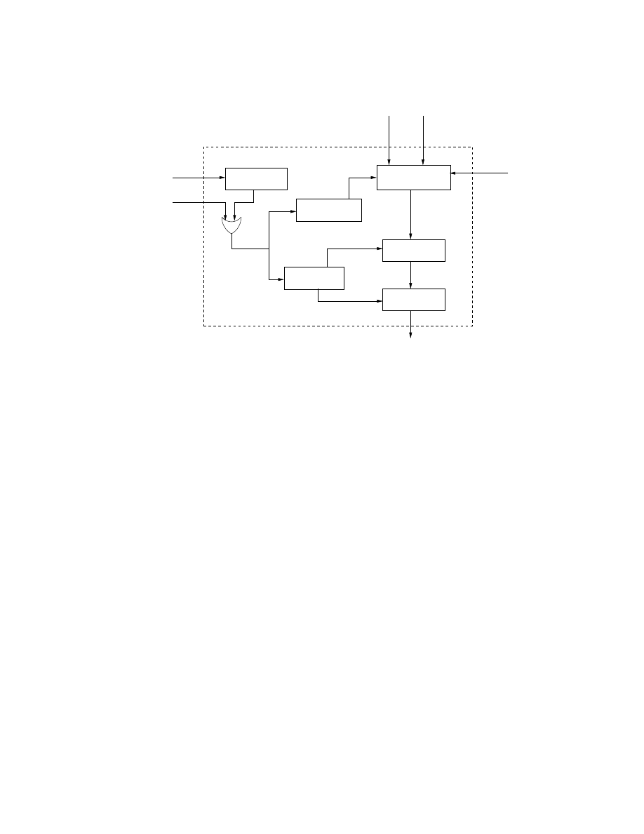
CHAPTER 3.

EVALUATION FRAMEWORK

NS to NS−testbed

Compiler

Event Control

System

Choose Worms

User Worms

Worm Library

User’s Defense

Program

Pseudo Vulnerable

Server

NS−testebed
Topology

EMULAB

Data Analysis

Tools

Evaluations

Worm Defense API

User’s

NS topology

User’s
Background Traffic

Figure 3.1: Design of the Worm-Defense Evaluator.

inserted into the appropriate event groups, such as, defense event group and vulnerable event

group respectively. This grouping is required so that the pseudo-servers and the defense

programs can be restarted from a single tevc command in the ‘Event Control System’.

This helps us to bring the testbed to a clean state instantaneously without swapping out

and swapping in experiments saving about 10–15 minutes. A clean state of the testbed is the

state when all experiment nodes are just booted up and no user processes are running, and

all changes made to the routing tables, firewall rules, IDS signatures, etc., during the last

run of an experiment are erased. Such a state is required for each run of an experiment. A

typical worm experiment series has about 1000–1500 experiments lasting two minutes each

on an average. This step helps complete a series in about 36 hours that would otherwise

take about twelve days. That is a huge saving!

3.3.2

Pseudo Vulnerable Servers

The ‘Pseudo Vulnerable Servers’, pseudo-servers for short, listen for traffic on a

certain port. Once they are receive a packet of a specified type, a worm packet, they mark

themselves as infected, save a time-stamp of the infection and spawn off a worm in their

own node. This relieves us of the task of writing a worm that exploits some vulnerability.

CHAPTER 3.

EVALUATION FRAMEWORK

By deploying our own pseudo-servers for vulnerable servers, we are also able to make use

of them as data acquisition tool.

This doesn’t compromise the experiment in any way. These pseudo-servers are a

valid abstraction of vulnerable servers because we don’t know how the real servers would

be attacked. Even if we write our own exploit for a real server, it will not reflect reality

as a real worm’s exploit is bound to be very different than the one we devise for our

experiments. Rather, we are more interested in worm spread models and ways to mitigate

the repercussions. Pseudo-servers accomplish these tasks effectively. We also note that,

these servers don’t take much time to spawn off a worm once they are infected. This is

not very different from real exploits which spawn off a worms in a victim machine rather

instantaneously.

As a pleasant side-effect, we end up with safe worms; worms that cannot spread

out on the Internet where these pseudo-servers are not installed.

3.3.3

The worm library

The framework has a very flexible built-in worm generator. This worm generator

can generate several families of worms based on the scanning pattern, transport protocol

used, and speed at which it scans for new victims. A worm in this library is specified by

the context-free grammar,

G = (V, Σ, R, hWORMi),

where the set of alphabets, Σ and the set of variables, V are respectively,

Σ = {0, . . . , 100, tcp, udp, random, topological},

V = {hTRANS PROTi , hSPEEDi , hNUMBERi , hSCAN ALGOi , hSCANOUT RATIOi}

and the rules, R, are:

hWORMi −→ hSCAN ALGOi hTRANS PROTi hSPEEDi

hSCAN ALGOi −→ random | topological hSCANOUT RATIOi

hTRANS PROTi −→ tcp | udp

hSPEEDi −→ hNUMBERi − {0}

hSCANOUT RATIOi −→ hNUMBERi

hNUMBERi −→ {0, . . . , 100}

CHAPTER 3.

EVALUATION FRAMEWORK

The available scanning patterns are random and subnet scanning. Either TCP or UDP

transport protocol can be selected and the scan speed is chosen as a number of scans

per second. SCANOUT RATIO gives the ratio of scans that go out of the sub-net for a

topological worm. The worm can be built with any given random string to act a payload.

However, this payload is discarded by the pseudo-server. So, a TCP sub-net scanning worm

that looks for a victim five times a second and send one out of every 10 scans out of the

sub-net can be specified as “topological 10 tcp 5”.

The worm itself has been implemented as a tight loop that sends out a message

every

scan rate

seconds, to the pseudo-server chosen according to its scanning algorithm.

The implementation provides for inserting any other third-party scanning algorithms into

the worm.

3.3.4

The Event Control System

The Event Control System(ECS) runs on the synchronization server of the exper-

iment. It controls the start and stop of the experiment run, triggering the data analysis

tools and rotating the log files.

This is a script that was hand-coded originally to help in evaluating our earlier

defense models. Now, we have parameterized this script so that others can also use it. The

parameters to the ECS are the worms that need to be launched, and the names of the event

groups generated by the compiler. These values are passed on to this component internally

transparent to the user.

When an experiment needs to be run, ECS starts all the program event groups.

Given the worm’s characteristics, the ECS bootstraps a worm on one of the pseudo-servers,

thereby creating victim 0. This starts the worm outbreak. The ECS keeps track of the

progress of the experiment by counting the time-stamps of the infections from the pseudo-

servers. (Since the same home directory is mounted on all experiment nodes all data is

written to the same directory and hence counting the time-stamps becomes easy as does

the final data processing). Once the worm count reaches a stable value the ECS deems that

the experiment run is complete. A worm count is considered stable if it does not change

for over a minute. The collected data is stored in a retrievable fashion. The event groups

are restarted and the next worm is launched. This is repeated for several pre-determined

iterations. Once the entire experiment series is complete data analysis programs are run on

CHAPTER 3.

EVALUATION FRAMEWORK

the collected data to give us the evaluations.

3.3.5

Data Analysis Tools

The pseudo-servers write all data on the user’s home directory. Current imple-

mentation collects infection time and alert time, the time when defensive responses kick in.

Tools are provided that chart the infection trace, the total number of nodes infected during

each experiment run and the time taken to stop the worm from spreading. The users are

welcome to do their own analysis of the data. In case, the user needs more data, the defense

programs need to be programmed appropriately to collect necessary information.

The next section presents an implementation of the framework which is encapsu-

lated in an Application Programming Interface(API).

3.4

The API

The framework described above has been implemented and a programming inter-

face has been provided. This API takes in three parameters, a network topology in NS [5]

format, a defense program and a worm. It returns a thorough analysis of the proposed

defense strategy based on various parameters. Some of these parameters are the total num-

ber of nodes infected, the time taken to stop the worm from spreading, the effects on the

network such as latency, bandwidth occupied by the defense vs the worm vs the normal

traffic, the effects of false alarms on the normal operational efficiency and the recovery time.

Recovery time is the time taken for the network to return from a defensive posture during

worm attack to its normal state of operation. This is a very important factor in real-world

networks because there is a cost involved when the network is not operating in its usual

fashion.

Figure 3.1 on page 29 gives a design diagram for this API. At the outset, we can

see that user specifies the above mentioned three parameters apart from the ability to play

background traffic using some third party tool. The following sub-sections describe the

user-inputs required and the various components of the framework.

CHAPTER 3.

EVALUATION FRAMEWORK

3.4.1

User Inputs

This sub-section describes the various user parameters and their specifications.

These are the topology specification, the worm parameters and the user’s defense program

and optionally a background traffic generator.

The topology specification

The user specifies the topology of the test network as an NS2 file. This would

represent the enterprise network of the user. The NS2 language was chosen because it lets

us specify exactly various network parameters like the network bandwidth, latency, etc., and

also allows for traffic shaping information. This topology information should also include

the location of various servers, gateways, routers, firewall, IDSes, etc., in the enterprise.

One can reconfigure the interconnection of the experiment nodes in EMULAB by

feeding it a script written in NS-testbed, an extension of the NS language. This extension

contains several commands that are specific to the testbed. These commands control the

event groups and program object sub-systems, the routing protocol used, the synchroniza-

tion sub-system, etc. The user’s topology is transformed into NS-testbed by the compiler

in our framework. This compiler will be discussed in the next sub-section.

The defense program

The API provides an interface to attach the users’ defense program to the frame-

work. Since users’ home directories are auto-mounted on all experiment nodes, there is no

need for any special installation procedures for these programs. It is sufficient if they are

available in the user’s execution path and the user just has to provide the program name.

Our compiler picks up this defense program and inserts it to the NS-testbed script thus

registering it with the testbed.

By providing such an interface, we allow for maximum flexibility for the user to

implement their own defense and response mechanisms. The programs could be anything

from worm detection algorithms using correlation, decision trees, Bayes Net techniques to

automatic signature generation to response mechanism using firewalls, IP black-listing, or

any other novel technology that the users’ want to evaluate. This is the parameter of the

API for which we expect the user to spend the most effort and rightly so because this is

the program we are evaluating.

CHAPTER 3.

EVALUATION FRAMEWORK

Since the defense program is already included in the defense event group by our

compiler, it would be called at the appropriate time from the Event Control System of our

tool. Ideally, we expect the user to design their defense program as a server that responds

to events, typically events that are symptoms of worm activity. Hence, the most propitious

time to start up these defense programs would be at the beginning of the experiment.

If the defense programs use any tools or programs that are not available by default

on the experiment nodes, these have to be installed manually and a disk image made prior

to starting the experiment. Then this image can be specified in the NS-testbed file to be

loaded on to the experiment nodes.

Worms Parameters

Our API by default provides a very parameterized worm generator. The parame-

ters are as follows:

1. Type of connection: UDP or TCP.

2. Speed of worm: The number of scans per second.

3. Scanning method: Random or subnet scanning. If subnet-scanning is specified the

user could also specify pods, the desired Percentage of Out-of-Domain Scanning. If no

pods is specified we use pods from 10 to 100 with step size of 10. In fact, at 100 pods,

the worm becomes a random scanning worm.

4. A payload to the worm: This could just be a random text. This is only to

analyze the effect of payload size on the worm dynamics and network bandwidth rather

than anything else. If it is a malicious function to be executed on the testbed, the

user should also provide the vulnerable servers along with the topology specification.

However, we discourage this, as this worm can get out of control and doesn’t add any

value to the experiments.

The users can choose one or more worms and parameterize them to be deployed

against their defenses. Alternatively, the API also provides hooks to hang the users own

scanning method for the worm. For example, a hit-list scanner, or a real Code-Red, Slam-

mer, etc. These user scan functions need to be added into the framework’s worm library

beforehand. Then the API should be instructed to use this users’ worm function while

choosing the ‘Scanning method’ mentioned above.

CHAPTER 3.

EVALUATION FRAMEWORK

After all, the users can just ignore all of these and provide their own worm programs

and corresponding vulnerable servers.

Background Traffic Generator

The users can replay their normal enterprise traffic in the background on EMULAB

while testing their defense policy. The background traffic can be played using tools like

TCPOpera [62] or NTGC [109] depending on whether the users want the traffic to be

source or trace parameterized. This may also depend on the defense strategies. If the

defense contains signature matching, the user may want to replay raw traces.

3.5

An Example - The Hierarchical Model of worm defense

To demonstrate the effectiveness of this tool, we consider a worm-defense model

called, The Hierarchical Model of worm defense that was developed in [33].

Briefly, this model assumes that all participating nodes are arranged in a tree

structure. The leaves are vulnerable but run some sort of an IDS system to detect attacks

and have some tunable firewall capabilities. The non-leaves are invulnerable to attacks and

run the worm-defense programs. Once a leaf detects an attack, it send a message to its

parent. In essence, this message would contain the suspicious packets. Once the parent

receives a threshold number of messages from unique children it takes two actions. One, it

instructs all its children to turn on responses to this attack. Two, it sends a message to its

own parent about the infection. Needless to say, for each non-leaf its threshold should be

lesser than its number of children to get any benefit from this scheme. Thus the information

about the attack travels up the tree and the instructions to respond percolates down the

tree. Intuitively, the lower the threshold, better the defense.

3.5.1

Modeling the system

The topology specification:

This model attempts to reflect a real enterprise network as

closely as possible. The root node would be entry point to the enterprise. The leaves would

be end-nodes, users machines and servers that are vulnerable to attacks. The non-leaf nodes

are routers or gateways to individual departments inside the enterprise.

Our experiments contained 4 levels in the hierarchy, representing the UCDavis’s

CHAPTER 3.

EVALUATION FRAMEWORK

College of Engineering network. Going down from the root to the leaves, each level rep-

resents, Gateway for the College of Engineering, the departmental gateways, research lab

routers and then finally the individual machines, in that order. This model consists of

pseudo-servers at the leaves running host based firewalls and IPSs that can be tuned upon

receiving instructions from their parents. All the non-leaves nodes run the defense program.

These nodes are called controllers because they control the defense. We also assume that

they are invulnerable to attacks.

This model is so simple that it can be represented by just the number of levels

in the hierarchy, the number of children and threshold of the nodes in each level of the

hierarchy. We hand-rolled a program that would read this specification and give us a NS-

testbed script. However, when we finally release the full implementation of this API, this

program would be a more versatile compiler to handle NS scripts.

The defense program:

The defense program is run on all the non-leaf nodes. Upon a

worm infection, the infected server would alert its parent. Once the threshold is reached,

the parent sends a similar alert to its own parent. In addition, it also extracts a signa-

ture from the suspicious packets received from its children. This signature is then sent to

its children including the infected ones, and instructs them to block traffic matching this

signature. Refer to [33] for further details of this model on back-off mechanisms, handling

false positives, etc.

The worm program:

Our experiments used the default worms provided by the frame-

work. UDP random and sub-net scanning worms were deployed against our defense using

a simple text string as the payload. No malicious programs were on the payload.

3.5.2

The experiment

All our nodes in the experiment ran FreeBSD 4.10 Jails. The controllers copied

the payload string into the signature distributed to the pseudo-servers. The latter in turn

implemented the defenses using a combination of firewall and IPS. “ipfw” was the firewall

of choice. This helped to divert packets arriving at a certain port to a program that could

examine them for the malicious signature. “snort inline” was the IPS of choice to examine

the packets and drop packets that matched the signature provided by the controllers.

Our tool ran the experiments with 160 pseudo-servers and 21 controllers in tree

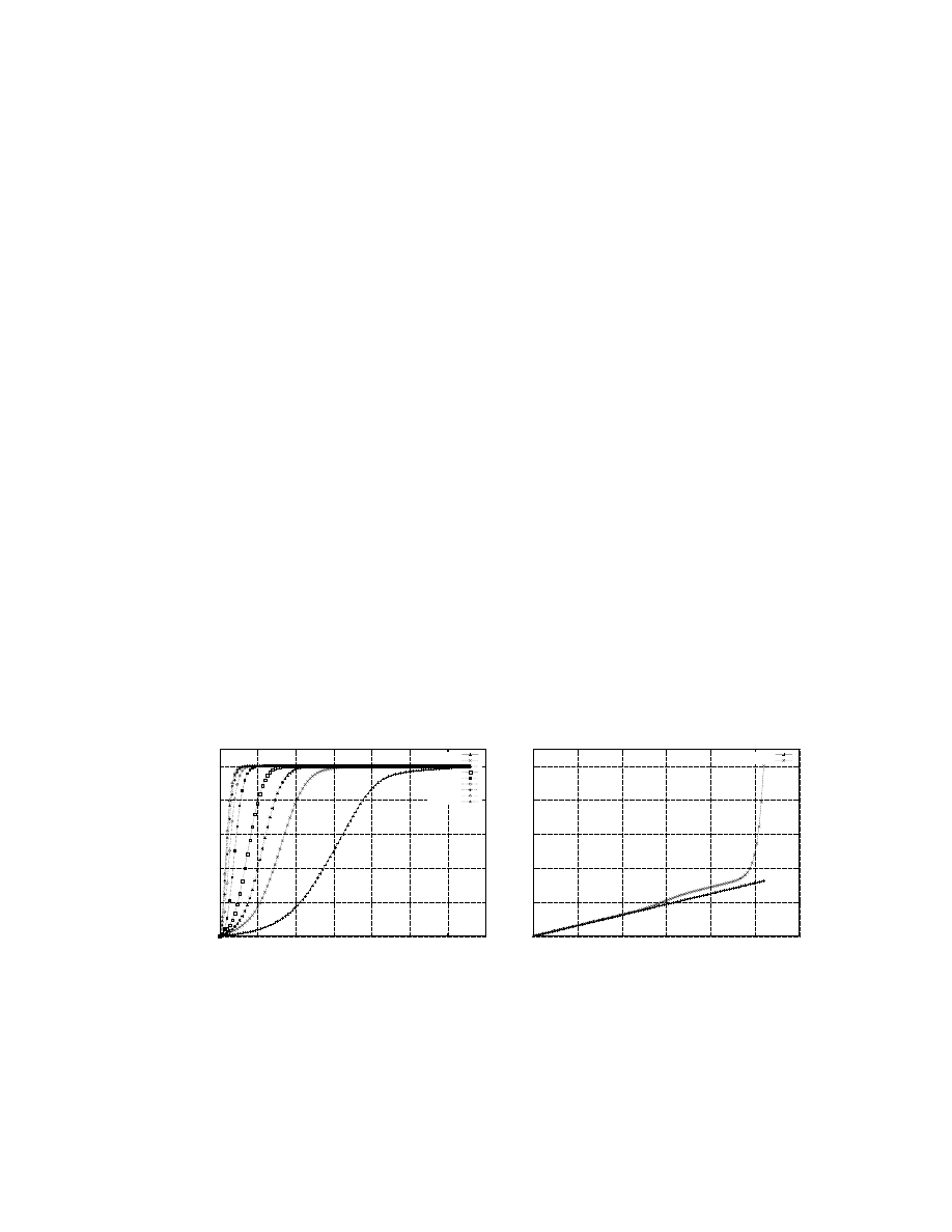
CHAPTER 3.

EVALUATION FRAMEWORK

topology with three layers. Each layer from the root of the tree contained one, four and

sixteen controllers respectively. We used both random scanning and sub-net scanning worms

with pods of 10–100. In fact, a subnet-scanning worm with pods of 100 is the same as a

random scanning worm. Each experiment was conducted with a worm of a particular

scanning speed. Different experiments were conducted with worms with different scanning

speeds in the range 0.2 to 100 scans per second. Each experiment was run for ten times, to

reduce the stochastic effects. This is not a large number but it did gave us better results.

Thus, ten different worm kinds at nine different speeds ran for ten repetitions making for

900 experiments. It took about 18 hours to complete it. This is where the diligence of this

tool comes to the fore. For sake of clarity, we only present the results of experiments with

pods of 30, 60 and 100.

First we corroborated our worm spread pattern with no defense to the mathemat-

ical models and simulation results [33]. The results of this run is shown in Figure 3.2(a).

This means that our worm program and the framework work as expected. Then we turned-

on the defense mechanism. Figure 3.2(b) shows how the defense overtakes the worm spread.

To recollect, the messaging protocol used here is hierarchical. Each node that sees a infec-

tion attempt sends an alert to its parent. Once the parent collects enough alerts to cross

a threshold, the alert is escalated to its parent. This continues all the way up to the root

node. We used a worm with a speed of 2 scans/second.

100

120

140

% of 160 nodes

Time(ticks)

worms 0.1
worms 0.2
worms 0.3
worms 0.5

worms 1
worms 2
worms 3
worms 6

worms 10

(a) Random scanning worms with no defense

100

% of 160 hosts

Time(ticks)

worms

alerts

(b) Alerts are distributed faster than the

worms

Figure 3.2: Notice the characteristics S-curve in Figure (a) on the left being flattened out
in Figure (b) on the right when the defense is turned on.

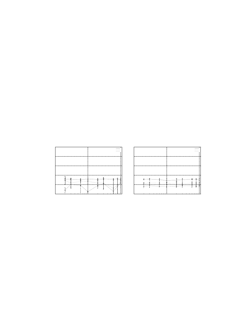
CHAPTER 3.

EVALUATION FRAMEWORK

3.5.3

Results

With the current set of experiments and the data analysis, we were able to draw

several insights into the hierarchical defense strategy. These are:

1. The root node alerts all of its children to turn on defenses within a definite time from

the first infection. All the experiments ran to completion. This shows that the system

is convergent and does not run-away due to any feed-back effects. This verifies the

mathematics given in Cheetancheri [33].

2. No matter how fast a worm spreads, this model of defense stops the worm with a

constant upper limit on the number of infections. This lets us decide the threshold

parameters at the controllers based on our tolerance for infections. Figure 3.3(b)

shows this result. Each data point shows the average number of infections and the

standard deviation.

100

% of 160 nodes infected

Worm speed

100 pods

60 pods
30 pods

(a) Only 5 iterations

100

% of 160 nodes infected

Worm speed

100 pods

60 pods
30 pods

(b) Increased to 10 iterations

Figure 3.3: The stochastic effects due to random variables are considerably less when the
number of iterations are increased.

3. The experiments showed us that this scheme works better for suppressing subnet-

scanning worms that are more biased towards scanning within the subnet than those

that scan outside the subnet. This also means this scheme performs poorly against

random scanning worms. Figure 3.3(b) shows this feature of the model. This is

obvious once we realize that alerts go out of the subnet faster than the subnet scanning

worms.

CHAPTER 3.

EVALUATION FRAMEWORK

4. Scale down factors: Figure 3.3(a) and 3.3(b) together show that the stochastic ef-

fects of scaling down of networks can reduced by increasing the experiment repetitions.

The experiment originally carried out with just 5 iterations gave us large standard

deviations, whereas the one with 10 iterations gave a considerably lower deviations

from the average value.

5. It is only the threshold levels that makes or breaks the network. A low threshold

helps to save a lot of machines but in reality it might help raise several false positives.

Figures 3.4(a) and 3.4(b) show the effect of different thresholds.

100

% of 160 hosts

Time(ticks)

50% Threshold

worms 2
worms 5

worms 10
worms 50

(a) Worm Containment with 50% Threshold

100

% of 160 hosts

Time(ticks)

75% Threshold

worms 2
worms 5

worms 10
worms 50

(b) Worm Containment with 75% Threshold

Figure 3.4: These two graphs show the relative performance of the defense for different
thresholds. Each node escalates an alert to its parent, when a certain percentage of its
children raise an alert.

3.6

Future work

Currently, the data analysis tools only analyze the kinematics of worms. We need

to design and implement the traffic analysis tools. As mentioned earlier, the effects on the

network such as latency, bandwidth occupied by the defense vs the worm vs the normal

traffic, the effects of false alarms on the normal operational efficiency needs to be analyzed.

For this, we need to design program stubs to be inserted at the appropriate locations on

the testbed.

In this chapter we presented only an operational work-around to counter the scale-

down effects on worm experiments. Two solutions to overcome this are to increase the ex-

CHAPTER 3.

EVALUATION FRAMEWORK

periment size and increase the number of iterations. Obviously, we can’t emulate the entire

Internet and we also can’t repeat experiments indefinitely. We need to find a compromise

between these two for our framework to be applicable to Internet wide worm problems.

We also want the users to be able to choose different kinds of networks from a

library. The library would provide a set of environments like university, a commercial or-

ganization or a defense network. There are differences between these networks. University

networks usually tend to be quite open with little or no firewalls enforced. It usually tends

to have several web-servers hosted by individual departments as well as individuals. A com-

mercial environment tends to be quite hardened on the outside but highly interconnected

on the inside. Companies also have trusted connections with their suppliers. A defense

establishment’s network tends to be highly compartmentalized with rigid firewalls on the

perimeter as well between different departments.

CHAPTER 4.

A DISTRIBUTED WORM DETECTION SYSTEM

Chapter 4

A Distributed Worm Detection

System

4.1

Introduction

Monitoring for and responding to security incidents in large-scale, complex enter-

prise networks requires a new approach to security incident management. Security reports

indicating a policy violation, come from a heterogeneous collection of components, such as

intrusion detection sensors, firewall access policy violations or anomalous network traffic

loads. Protecting against attacks currently in progress or eliminating a new vulnerability

involves the reconfiguration of several different types of devices, such as firewalls, border

gateways, software updates, and even host-based wrappers.

The challenge is to collect all information from the numerous data sources and to

decide on appropriate actions for each reactive component. Simply forwarding all reports

to a central location will not scale to large networks. Local decision making, however, may

lack the global view necessary to thwart large-scale attacks.

Defending against worms, particularly day-zero worms, is perhaps the most press-

ing challenge for a large enterprise. Such a worm can have a devastating impact as it

automatically propagates itself to all vulnerable machines on a network. Defending against

worm attacks, for which no pre-existing attack signature is available, requires the automa-

tion of tasks that current system administrators must perform manually. These include:

automatic aggregation and correlation of security reports to detect activity at a local site,

CHAPTER 4.

A DISTRIBUTED WORM DETECTION SYSTEM

automated short-term defensive actions to stop local worm infections, cooperative alert

sharing across administrative boundaries to protect sites not yet infected, and automated

back-off when a worm is contained or in the event of a false alarm.

4.2

A Distributed Collaborative Defense

As a complement to centralized cyber-security defensive systems we have developed

and evaluated cooperative defensive schemes. Centralized systems are designed primarily

to protect enterprises by monitoring aggregate traffic at fixed locations in the network and

responding by blocking or delaying observed malicious behavior. In some circumstances,

however, such centralized systems may not be suitable; organizations may not have the

resources to acquire and manage a large system, there may not be sufficient trust between

sub-domains to accept a centralized protection policy, and large numbers of mobile nodes

may exit and enter the network leaving them temporarily without protection.

Previous work by us and others [13,26,28,48] have developed cyber-defenses based

upon collaborative alert-sharing as a way to detect and react to large-scale distributed at-

tack such as Internet worms. Evaluation of these schemes is usually done both analytically

and through simulation. Assumptions regarding false positive rates and other environmen-

tal aspects are idealized abstractions due to the lack of a realistic testing and evaluation

framework. Emulations on DETER and Emulab testbeds were used for this work.

4.2.1

Collaborative Distributed Attack Detection

In this chapter we describe and evaluate a scheme for distributed attack detec-

tion using cooperating end-hosts. In this system, all events are generated using software

detection agents on individual end-hosts. Currently, we monitor inbound and outbound

network traffic at the host and detect local anomalies in traffic features. Due to the limited

view of these detectors, however, isolated end-hosts alone would serve only as low-quality

(high false positive or high false negative) detectors of distributed attacks. Our goal is to

cooperatively share information such that the aggregation of end-host alerts produces a

high-quality (low false positive and low false negative) global attack detector. We accom-

plish this by implementing a distributed version of the sequential hypothesis test(dSHT)

used successfully in centralized detection schemes [64]. With this method, all collaborating

sites maintain a decision table constructed using the ratio of the likelihood that the features

CHAPTER 4.

A DISTRIBUTED WORM DETECTION SYSTEM

are a good indicator of the current worm attack to the likelihood for the features to occur

at random. When the likelihood of observed behavior exceeds a predetermined threshold,

enough evidence has been accumulated to reach a correct decision with high probability.

This work was inspired by the Jung et al.’s algorithm for quick port-scan detection

[64]. While they use Sequential Hypothesis Testing to identify malicious port-scanners, we

adapted the principle to detect worms. In this formulation, let H

and H

be the hypotheses

that there is and is not a worm respectively. Let Y

be the random variable that says there

is evidence of an attack or not at site i. This represents the weak local end-host detector

at site i.











1 if there is evidence of an attack;

this could be either an attack or a false positive with probability(fp)

0 if there is no evidence of an attack;

this could either be an attack or a false negative with probability(fn)

By definition,

P[Y

= 0|H

] = fn; P[Y

= 1|H

] = (1 − fn)

P[Y

= 1|H

] = fp; P[Y

= 0|H

] = (1 − fp)

The observation vector ~

Y = {Y

, Y

· · · Y

} then is the set of measurements ob-

tained by n conditionally independent end-hosts. Each end-host contributes one y

to the

vector and passes the vector to another end-host as dictated by the messaging protocol in

effect at that time. Sec. 4.2.2 details the messaging protocol we used in this study. We now

define, P [~

Y |H

] to be the likelihood that the given observation ~

Y was made because the

hypothesis H

is true. Therefore the ratio,

L(~

Y ) =

P[~

Y |H

]

P[~

Y |H

]

gives the Likelihood Ratio that the sequence of events observed are a good indicator of the

current worm to the likelihood for the observation to occur at random. Further assuming

all Y

’s are conditionally independent measurements, we have,

L(~

Y ) =

P[Y

] · P[Y

] . . . P[Y

]

P[Y

] · P[Y

] . . . P[Y

]

for a sequence of n local detectors sampled. Then if vector ~

Y has a 1’s and b 0’s, the

Likelihood ratio is,

L(~

Y ) =

(1 − fn)

∗ fn

∗ (1 − fp)

CHAPTER 4.

A DISTRIBUTED WORM DETECTION SYSTEM

Using this we compute a table of the outcomes of many random walks through a collection

of local detectors. For example, entry (5,2) would contain the likelihood ratio of finding

two alerts after sampling five independent sites.

The strength of the desired global detector, then, is specified by two quantities:

desired detection rate, DD, and desired false alarm rate, DF . DF , in other words, is the

maximum acceptable failure rate of the global detector. Using these, one can calculate

thresholds in the table of likelihood ratios:

T 0 =

1 − DD

1 − DF

and T 1 =

Each host, then, implements a global intrusion detector that makes decisions as

follows: if, after including the local detector state, the calculated likelihood ratio, L( ~

Y ),

is less than T 0, accept the hypothesis that there is no worm (H

) and halt the query. If

L(~

Y ) > T 1, accept the hypothesis that there is a worm (H

) and raise a global alarm,

otherwise continue the random walk among end-hosts. This defines upper and lower blocks

in the decision table as a region likely to have been produced by an attack and a region likely

to come from normal behavior. By independently sampling weak local end-host detectors

with given fp and fn, one can achieve a strong global detector if enough sites are traversed.

4.2.2

Cooperative Messaging Protocols

In the scheme described above, the method for obtaining random samples from

cooperating end-hosts is left unspecified. In the case of Internet worm attack, our initial tests

were performed using an epidemic spread protocol. Cooperating hosts contain a random

subset of the addresses of all nodes in the collection. Nodes with new alerts from their local

detectors choose m other end-hosts at random and send the message “{1, 1}”, which means,

“one site has reported one alert”. Hosts receiving this message add their local information

(e.g. it would generate a “{2, 1}” if had not seen the activity, and a “{2, 2}” if had) and

attempt to arrive at a decision based upon the table of likelihood ratios. If no decision is

reached, m new sites are selected at random and the message propagates. In this manner

multiple SHT sequences(chains) of evidence are spread randomly across cooperating end-

hosts. If “normal behavior” decisions are reached in any chain, that chain halts. If a “likely

worm attack” decision is reached at any point, a global warning is broadcast to all nodes.

Figure 4.1 shows an example message chain with a fan-out, m = 2. Preliminary experiments

on Emulab [120] and DETER [16] testbeds have led us to conclude that messaging overheads

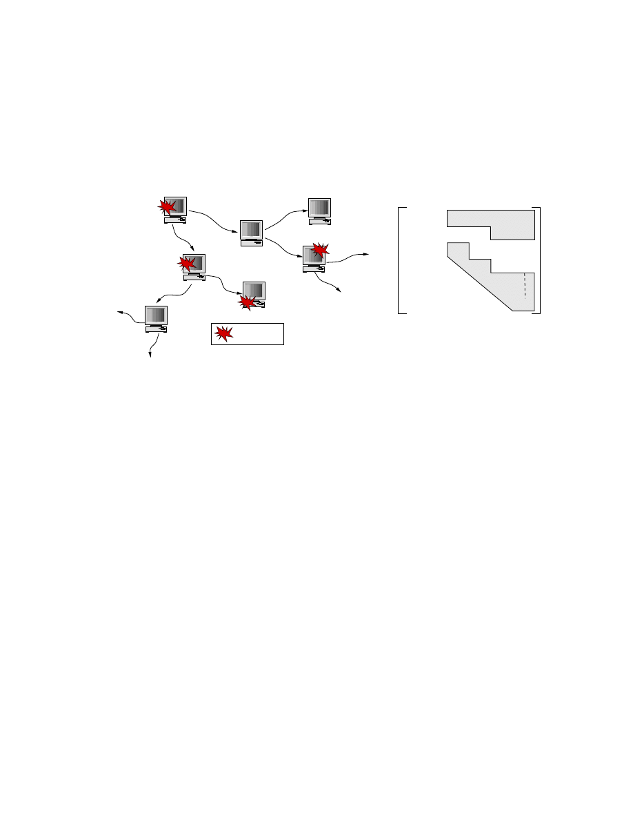
CHAPTER 4.

A DISTRIBUTED WORM DETECTION SYSTEM

for protocols with m > 1 provide little benefit in early detection and result in needless

communications in the presence of local false positives. During times of widespread attacks

multiple query chains are initiated by local detectors, forming an ever-increasing number of

independent queries.

Local Alert

WORM!

{3, 3}

{3, 2}

{3, 1}
No Worm

{2, 2} {3, 2} {4, 2} . . . {n, 2}

{3, 3} {4, 3} . . . {n, 3}

{4, 4} . . . {n, 4}

{n, n}

{1, 1} {2, 1} {3, 1} {4, 1} . . . {n, 1}

No Worm

WORM!

Global Decision Table maintained at each site

{i, j} = j local alerts seen after i steps

{2, 2}

{1, 1}

{2, 2}

{3, 2}

{2, 1}

{3, 2}

Figure 4.1: Diagram illustrating the co-operative messaging protocol and the decision table
used in dSHT used to generate a global worm detector

4.3

Evaluation on an Emulated Test-bed

One major difficulty in testing any large-scale defensive systems is that a large

number of test machines have to be configured and managed efficiently. To accomplish these

tasks, we used the Emulab and DETER testbeds along with evaluation framework developed

in the previous chapter. Instead of the native worm libraries and pseudo-server(Fig. 3.1)

we used a more powerful worm simulation engine called WormSim [81] and its companion

XML worm-specification library.

4.3.1

Experimental Setup

The goals of our experiments are to evaluate our algorithms’ effectiveness in iden-

tifying worm outbreaks, to determine its robustness against false alerts and to measure the

network overhead of the cooperative protocol itself.

The major components of our current experiment setup are:

• A worm simulator engine(Wormsim)

CHAPTER 4.

A DISTRIBUTED WORM DETECTION SYSTEM

• A local intrusion detection system (IDS) to generate low level sensor inputs.

• A global detection algorithm and protocol implementing dSHT.

• The evaluation infrastructure including the network test-bed itself and instrumenta-

tion tool-kits.

We describe these components briefly.

Wormsim

To test distributed defenses in the presence of realistic worm attacks with-

out installing vulnerable software, we developed the Wormsim worm emulation framework.

The goal of this framework is to generate network traffic patterns that mimic, as closely

as possible, the patterns generated if malicious code had actually existed on the end hosts.

Rather than executing malicious binary instructions that govern worm propagation, Worm-

sim agents interpret XML specifications written to emulate the same behavior. Agents ac-

cept and parse messages in an XML format and then, based upon the specification, connect

to other “victim” hosts, sending them the same XML worm instructions. The targets are

identified based upon the parameters in the XML worm specifications. Some other features

that can be specified are the scan method, the transport protocol to use, the scan rate, etc.

Each Wormsim engine can be remotely configured to be either vulnerable or not vulnerable

to a particular worm.

A Local IDS

In tune with our philosophy of achieving high-confidence correlations from

weak detectors, we implemented a very weak end-node IDS. The IDS would raise an alarm

to trigger dSHT whenever there is a connection attempt to an un-serviced port. The

reasoning is that, a legitimate connection attempt usually never goes to a host that does not

service it. On the contrary, automated attacks such as worms, ignoring sophisticated ones

that have information from prior reconnaissance, try to make connections indiscriminately.

Thus, those nodes that service a certain port have no protection and do not trigger the

SHT. However, IDSes used in practice are much better than the one we use and will help

in detecting a more sophisticated attack. This will enable even the vulnerable nodes to

participate in the protocol.

Since Wormsim knows the vulnerability status of the host at a certain port, it can

easily use the event of receiving XML specifications on a non-vulnerable node to trigger the

detection algorithm. Hence this IDS was implemented as a patch to Wormsim itself.

CHAPTER 4.

A DISTRIBUTED WORM DETECTION SYSTEM

Global Detection Algorithm

As a message propagates, each detection agent adds one

to the number of nodes queried and one to the number of positives if it has seen a similar

alert locally. At this time, we assume there is only one alert that can be raised and hence

no information about the kind of attack is passed along. However, we envision using an

anomaly vector in future to describe the event so that stronger correlations can be made.

The SHT parameters DD and DF were set to 98% and 2% respectively(sec. 4.2.1).

We consider these values to be within reasonable tolerance. The local IDS miss rate, fn, was

set at 1%. Their false alarm rate was the independent variable and chosen as described in

the next section. The fan-out, m, for the co-operative alert protocol (sec. 4.2.2) is set to 1.

With each new infection, one new SHT sequence is created. After the first few infections,

there are multiple parallel global alert chains propagating simultaneously. Each member

propagates an alert by sharing it with another randomly chosen member. Besides satisfying

a basic requirement for the SHT algorithm, such random selection defends the protocol

from the following two attacks. One, malicious members gaming the protocol. Two, clever

or hit-list worms, or a combination of both, circumventing our protocol by targeting only

those nodes that will not be chosen to share the alert.

Evaluation Infrastructure

The experimental test network was configured with 100 PCs,

a mixture of Pentium IVs and 64-bit Xeons randomly assigned by the testbed, running

FreeBSD 4.10. All nodes were assigned to a single LAN, though we emphasize that we

could have used several thousand machines. Each one of them can be as far away from each

other on the Internet and only connectivity amongst the nodes matter. We also emphasize

that we are not trying to save the entire Internet from the worm attack. We are only

interested in an early detection for this particular federation of willing participants.

A 1Mb LAN was used so that test machines on different switches could be assigned

to our experiment. This speeds up node assignment on the testbed to our experiment

without significant changes in experimental results since our cooperative protocol was not

expected to consume much of the total bandwidth.

4.4

Experimental Results

To evaluate our system we focused upon three primary properties: the ability of

the algorithm to detect worms, the likelihood of generating a global worm alert for a given

CHAPTER 4.

A DISTRIBUTED WORM DETECTION SYSTEM

level of local false alarms, and the messaging overhead of the system under various false

alarm conditions.

4.4.1

False Alarm Experiments

We wish to answer the following two questions in these experiments:

1. How many simultaneous false alarms generated by the local IDS are required to

wrongly choose hypothesis H

, a global false alarm?

2. What is the network bandwidth overhead during normal operating conditions?

Wrong Choice:

The answer to first question is important due to the following reason.

Since, the local host IDS operates on a very na¨ıve principle, we expect to initiate cooperative

chains conducting the SHT quite frequently and even when there are no worms. Each and

every local false alarm, or even a malicious port scan, will initiate a query sequence. To

answer this question we set-up the following experiment.

Each local IDS was assigned a certain false alarm rate fp denoting its quality;

(i. e) for each IDS, a certain n alarms out of every 100 was considered to be spurious.

This property of the IDS forms an input to constructing the the decision table used by each

participant. We set n ∈ {1, 3, 5, 10, 20}. n takes one of these five values for each experiment.

An IDS with n = 1, or equivalently f p = 0.01, is said to be of high quality while one with

n = 20 is considered to be poor.

It would be impractical to use the false alarm rates, configured as a parameter

of the local detectors, to generate sensor events in the test-bed experiment. If we were to

wait for, say, five simultaneous false alarms, most of the experiment time would be spent

in simply waiting for this rare event. Alternatively, we selectively generate the rare events

themselves and record the effects of these events on our SHT algorithm. The goal here

is to generate simultaneous false-alarm conditions so that a SHT sequence has multiple

members that have seen a local false alarm. We use the Event Control System (ECS) of the

emulab test-bed to trigger false alarms in a number of participants(m) simultaneously. We

set m ∈ {3, 5, 10, 20}. m takes one of the four values in each experiment described below.

The results can then be applied to systems with a given quality of IDS.

Thus, we have a family of 20 experiments with different configurations (m simul-

taneous false alarm conditions times n local IDS quality levels) to run. We repeat each

CHAPTER 4.

A DISTRIBUTED WORM DETECTION SYSTEM

experiment 20 times to reduce the effects of random fluctuations. These experiments were

conducted with the detection system running on all 100 nodes. Wormsim did not have to

generate any worms during these experiments.

0.2

0.4

0.6

0.8

False Worm detection fraction

# of simultaneous false alarms

Performance under false alarms

Quality of IDSs

1%
3%
5%

20%

(a) H

chosen wrongly due to false alerts

# of messages

# of simultaneous false alarms

Network traffic overhead

Quality of IDSs

1%
3%
5%

10%
20%

(b) Total number of messages required before

dSHT chooses one hypothesis over the other

Figure 4.2: False alarms experiments

Fig. 4.2(a) shows the number of local false alarms needed to generate a global false

alarm. It shows the fraction out of 20 repetitions of the experiments the dSHT wrongly

chose hypothesis H

. Naturally the the incidence of this mistake goes up as the number of

simultaneous false alarms increases. However, the global detector raises fewer false alarms

when the local IDS raise more false alarms. For example, for a very poor quality local host

IDS (with a 20% fp) the dSHT algorithm makes the global detector highly suspicious of

alerts received resulting in fewer mistakes.

For the higher quality local host IDS, five simultaneous false alarms will wrongly

produce a global worm alert using 15% of the time. While this may not seem particularly

small, the chance of getting 5 simultaneous false alarms is highly unlikely to begin with

because the IDS quality is set to be high.

Network overhead:

The concern that raises the second question listed above is that if

the local host IDS quality is too low, during normal operations, dSHT would require an

excessive number of queries in each chain before either hypothesis is chosen to be accepted.

In essence, the path taken in the decision table would remain in the middle, undecided

CHAPTER 4.

A DISTRIBUTED WORM DETECTION SYSTEM

portion rather than reaching any decision.

Were this to happen continuously it might adversely affect network operations or

allow a sophisticated attacker to trigger minor false alarms to deliberately induce periods

of high bandwidth message passing. Fig. 4.2(b) shows the number of messages required to

choose either hypothesis for four different environments(indicated by the ambient levels of

simultaneous false alarms) and for five different qualities of the local end-host detectors. The

numbers are averaged over 20 experiments. The maximum standard deviation observed was

3.2 messages; when 20 false alarms were fired simultaneously from end-node IDSes whose

fp rates were pegged at 3%.

The number of messages increases in proportion to the number of simultaneous

false alarms since each false alarm initiates a new query chain. The number of messages,

however, depends little on the quality of the local end-host IDS. During periods of false

alarms, since the local alerts are independently distributed across end-hosts (next hop neigh-

bors are selected at random), decisions are reached regarding false alarms after querying

only four end-hosts on average. There seems to be little danger here in a runaway dSHT

causing harm to normal network operations, even when the local end-host detectors are

relatively poor.

4.4.2

Performance in Detecting Worm Attacks

The second set of experiments was performed to test the system’s response in the

presence of self-propagating worm attack. We do not study the effects of false alarms in

presence of worm traffic as it would only help to make a “worm” decision sooner. For

our worm experiments we set the vulnerability density to be 25%(i. e) one-fourth of the

participant are vulnerable; a random process chooses which specific nodes in the test-bed

are vulnerable. We configured the worm to send out a random subnet scan every 1 second.

Since the entire vulnerable population is on one subnet, this worm is effectively a random

scanning worm. The worm scan speed does not have any impact on detection unless it is

faster than the detection algorithm. The morphology of the worm is also not of concern as

we do not deal with worm semantics. We only exchange much coarser information about

anomalies.

We want to determine the effect of various local end-host IDS quality on decision

time and infection rates. Thus, we have n experiments to run against this worm; one for

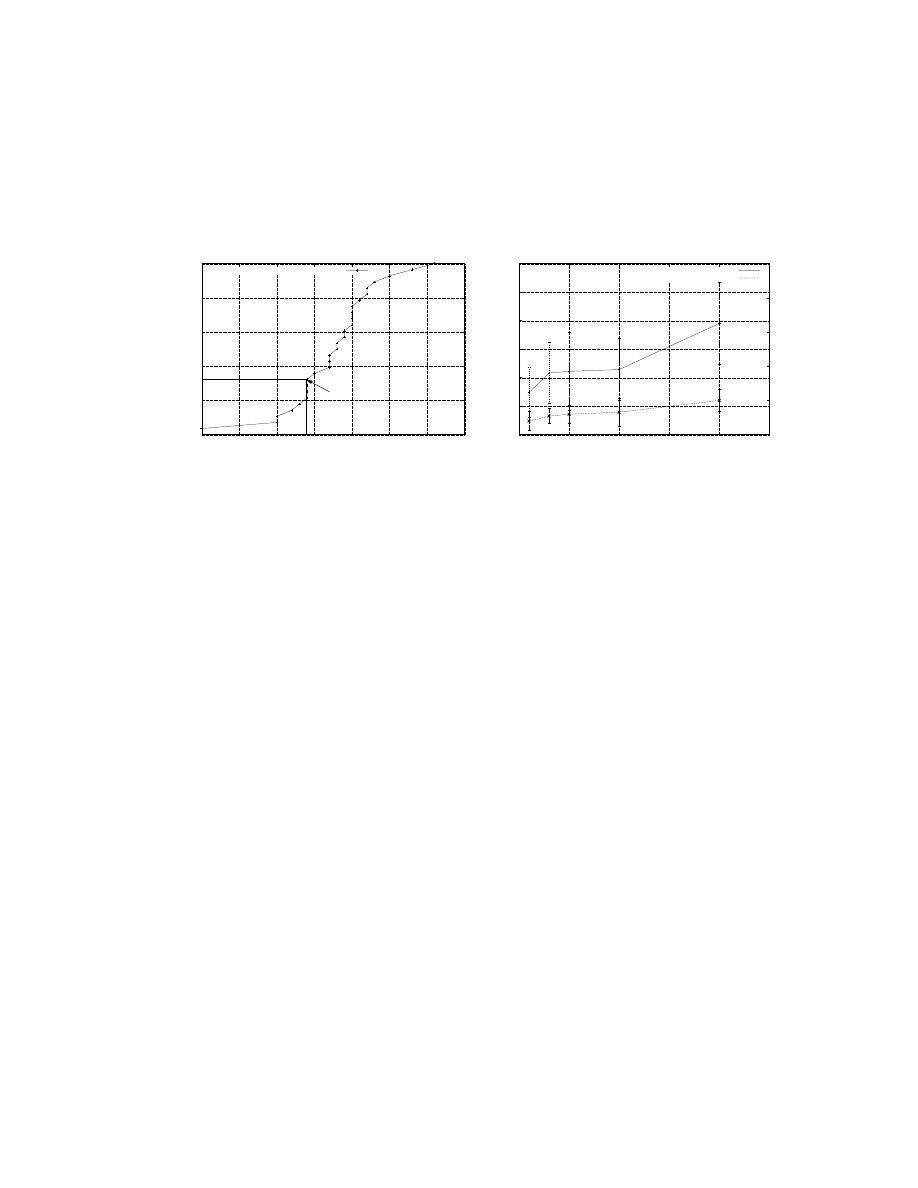
CHAPTER 4.

A DISTRIBUTED WORM DETECTION SYSTEM

each end-host IDS quality. We again repeat this experiment 20 times to reduce the effects

of random fluctuations.

100

% of vulnerables infected

Time (s)

Sample worm and detection (IDS fp rate = 10%)

Worm detected

Random Scanning worm 1 scan/s

(a) A sample infection sequence and detection

instant

% vulnerables infected

Time to detection

Quality of IDSs (fp rates)

Time to true worm Detection

% Infected

Time to Detection(s)

(b) Results from all worm experiments show-

ing the percentage of infected nodes at detection

time as a function of local end-host IDS quality

Figure 4.3: Worm experiments

The results from a typical worm attack experiment are shown in Figure 4.3(a).

The percentage of vulnerable machines infected is plotted as a function of time and exhibits

the characteristic s-curve infection profile. In this example, the decision table is constructed

using a 10% false alarm rate in the end-node detectors. At this rate, a worm decision is

reached at 14 seconds after the launch of the attack with 32% of the vulnerable nodes

already infected. Since the local end-host IDS in this case is rather poor, a decision is not

reached until relatively late in the infection profile.

Detection times and percentages of infected hosts from all experiments were col-

lected and are shown plotted together in Figure 4.3(b). We notice that the number of

infections before worm-detection increases with decreasing quality of end-node detectors.

While poorer quality end-host detectors do not necessarily lead to larger problems with

respect to false alarms, they have a significant impact on the global dSHT detector’s ability

to quickly detect worms; before unacceptable numbers of vulnerable nodes have been com-

promised. Since the global dSHT must be more tolerant to high levels of false alarms, it

takes longer to claim a worm with the required high levels of confidence. However, there are

no cases of missed worms. Sooner or later, worms are always detected. Only those worms

CHAPTER 4.

A DISTRIBUTED WORM DETECTION SYSTEM

that carefully avoid all non-vulnerable nodes will not be detected. However, as mentioned

earlier in section 4.3.1, IDSes used in practice are much better than the one we used and

can detect more sophisticated attacks enabling even the vulnerable nodes to participate in

the protocol.

4.5

Future Work

There are quite a few important aspects that we still need to address. A couple of

them are listed below.

We need to define the anomaly vector to share amongst the detection agents. Some

of the features of this vector could be a flag to indicate presence of machine instructions in

traffic to servers, the size of such instruction sequences, the frequency of such connection

attempts, the recent CPU usage statistics, etc.

In our current study we have not taken into consideration the effect of the worm

traffic from outside our network of interest. To address this, we are developing an Internet

scale-down node. This node represents the Internet external to our network and would

generate traffic into our emulation network based on the mathematical model of the worm

specification. We may be able to make use of the work done by Liljenstam et al. [78] for

this. Evaluating dSHT in the presence of traffic from this Internet Scale-down node forms

our next step in this direction.

We have also not considered the effects of malicious nodes in the federation in

these experiments. To overcome such problems, we could introduce several variations in the

protocol. For example, instead of declaring ’worm’ immediately after the first such decision,

we could wait until a certain number of unique participants make the same decision. It is

worth noting that a similar problem has already been formulated and solved by the systems

community as the Byzantine Generals problem [12, 72, 89]. Those solutions might help

alleviate this problem at the cost of using more network bandwidth and a delayed detection.

CHAPTER 5.

RESPONSE USING DYNAMIC PROGRAMMING

Chapter 5

A Dynamic Programming

Formulation for Worm Response

5.1

Introduction

Dealing with known worms is a solved problem – signatures to be used by Intru-

sion Prevention Systems(IPSs) are developed to prevent further infections, and patches are

developed to fix vulnerabilities exploited by these worms. Dealing with unknown worms –

worms that exploit zero-day vulnerabilities or vulnerabilities for which patches have either

not been generated or not applied yet – is still a research question. Several ingenious pro-

posals to detect them automatically exist. Many of them have also proposed sophisticated

counter measures such as automatic signature generation and distribution [70, 98, 114] and

automatic patch generation to fix vulnerabilities [103].

Often times, even if automated, there is not much time to either generate or

distribute signatures or patches. Other times, system administrators are skeptical about

applying patches. During those instances when such automatic signature based traffic

filtering or patching are not feasible, the only option left is to either completely shut-down

the vulnerable service or keep it running risking infection. It is usually preferred to shut-

down the service briefly until a mitigating response is engineered to the worm.

However, making this decision becomes hard when one is not completely sure if

there is really a worm, and if the service being offered is vulnerable to it. It does not make

much sense to shut-down a service and later realize that such an action was not warranted.

CHAPTER 5.

RESPONSE USING DYNAMIC PROGRAMMING

Whereas suspending the service in an attempt to prevent infection is not considered bad.

Intuitively, it is desired to shut-down the service briefly until it is clear whether there is an

attack or not. Balancing the consequences of providing the service risking infection against

that of not providing the service is of the essence.

This chapter captures this intuition and devises an algorithm using Dynamic Pro-

gramming(DP) techniques to minimize the overall cost of response to worms where cost is

defined as some mathematical expression of an undesirable outcome.

These algorithms use information about anomalous events that are potentially due

to a worm from other co-operating peers to choose optimal actions for local application.

Thus the response is completely decentralized.

We surprisingly found that for certain scenarios, to leave oneself open to infection

by the worm, might be the least expensive option as demonstrated by our algorithms. We

also show that these algorithms do not need a great deal of information to make decisions.

5.2

Dynamic Programming

The basic model of a system consists of two main features: (1) a discrete-time

dynamic system and (2) a cost function that is additive over time. The system has the form

= f

, u

, w

k = 0, 1, . . . , N − 1

(5.1)

where

k indexes discrete time,

is the state of the system and summarizes past information that is relevant for future

optimization,

is the control or decision variable to be selected at time k,

is a random parameter, also called disturbance or noise depending on the context,

N is the horizon or the number of times control is applied.

and f

is the function that describes the system and in particular the mechanism by which

the state is updated.

CHAPTER 5.

RESPONSE USING DYNAMIC PROGRAMMING

The cost function is additive in the sense that the cost incurred at time k, denoted

by g

, u

, w

), accumulates over time. Thus the total cost is

) +

−1

, u

, w

)

where g

) is a terminal cost incurred at the end of the process. However, because of

the presence of a random parameter, w

, the cost is generally a random variable and cannot

be meaningfully optimized. We therefore formulate the problem as an optimization of the

expected cost

(

) +

−1

, u

, w

)

where the expectation is with respect to the joint distribution of the random variable in-

volved. The optimization is over the controls u

, u

, . . . , u

−1

, and each control, u

, is

chosen based on the current state of the system, x

. This is called closed loop optimiza-

tion as opposed to open loop optimization when all controls have to be decided at once at

time 0 without any knowledge of the state of the system at any time later.

Mathematically, in closed-loop optimization, we want to find a sequence of func-

tions, µ

, k = 0, . . . , N − 1, mapping the system state x

into a control u

which when

applied to the system minimizes the total expected cost. Thus u

← µ

). The sequence

π = {µ

, . . . , µ

−1

} is referred to as a policy or control law.

For each policy, π, the corresponding cost for a fixed initial x

is denoted by J

We want to minimize this for a given x

over all policies that satisfy the constraints of the

problem. The policy that does this is denoted by π

∗

and minimizes the corresponding cost,

∗

). However, it is also possible to find the policy that minimizes the cost for any x

An introduction to a few notations are in order now. We denote by J

) the

cost-to-go from state x

at time k to the final state at time N . Thus, J

) is the terminal

cost and J

) = J

) is the total cost.

Dynamic Programming Algorithm:

An optimal total cost is given by the last step of

the following algorithm, which proceeds backwards in time from period N − 1 to period 0:

) = g

(5.2)

) = min

, u

, w

) + J

)

k = 0, 1, . . . , N − 1,

(5.3)

CHAPTER 5.

RESPONSE USING DYNAMIC PROGRAMMING

where the expectation is taken with respect to the probability distribution of w

, which

depends on x

and u

. Furthermore, if u

∗

minimizes the right side of equation (5.3) for

each x

and k, the corresponding policy π

∗

is optimal.

5.3

DP Problems with imperfect state information

In this section, we first describe DP problems involving imperfect state informa-

tion. Then, we show how these can be transformed into problems with perfect state infor-

mation through state augmentation. We then list down the complexities involved in solving

such problems. In the next section, we will formulate worm response as a DP problem with

imperfect state information. We also explain how and why the complexities involved in

such formulations do not affect the worm response problem.

5.3.1

Problem Description

Often, information about the exact state of the system, x

is not available. Instead,

only a certain observation, z

, about the system state is available. The observation takes

the form:

= h

, v

= h

, u

−1

, v

k = 1, 2, . . . , N − 1,

(5.4)

where v

is the observation disturbance and characterized by a given probability distribution

(.|x

, . . . , x

−1

, . . . , u

−1

, . . . , w

−1

, . . . , v

The initial state x

is also random and has a probability distribution P

. The probability

distribution of w

may depend on the state of the system and the control but not the prior

state disturbances, w

−1

, or observation disturbances, v

−1

. The control u

is constrained

to take values from a given nonempty subset U

of the control space. It is assumed that

this subset does not depend on the x

Let us denote by I

the information available to the controller at time k and call

it the information vector. We have

= (z

, z

, . . . , z

, u

, . . . , u

−1

k = 1, 2, . . . , N − 1

= z

(5.5)

CHAPTER 5.

RESPONSE USING DYNAMIC PROGRAMMING

Analogous to the basic model of a dynamic programming problem in section 5.2, we

want to find an admissible policy π = {µ

, µ

, . . . , µ

−1

} that minimizes the cost function

=0,1,...,N −1

(

) +

−1

, µ

), w

)

subject to the system evolution

= f

, µ

), w

k = 0, 1, . . . , N − 1,

and the measurement equations (5.4) in which u

−1

is replaced by µ

−1

5.3.2

Re-formulation as a Perfect State-information Problem

In the absence of precise information about the state of the system, it is intuitively

clear that we need to define a new augmented system whose state at the time k would

contain information about all the variables that can help the controller while making the

kth decision [22]. The information vector I

forms an ideal candidate to describe the state

of the new system. By definition of I

in equations (5.5), this new system can be defined

to evolve as:

= (I

, z

, u

k = 0, 1, . . . , N − 2,

= z

(5.6)

where, I

describes the state of the system, u

is the control as usual while z

can be

treated as the random disturbance as it is dependent on a random variable v

as mentioned

in equation (5.4).

The cost incurred during the kth stage is now:

, u

) =

, u

, w

)|I

, u

(5.7)

Thus the problem with imperfect state-information has now been reformulated as a perfect

state-information problem with the augmented system evolution (5.6) and augmented cost

per stage (5.7). By writing out the DP algorithm (5.2) and (5.3) for the above system, we

get:

−1

) = min

N −1

−1

, u

−1

, w

−1

)

+ g

−1

, u

−1

, w

−1

)|I

−1

, u

−1

(5.8)

CHAPTER 5.

RESPONSE USING DYNAMIC PROGRAMMING

and for k = 0, 1, 2, . . . , N − 2, we have:

) = min

k+1

, u

, w

) + J

, z

, u

)|I

, u

(5.9)

These equations form the DP algorithm for the reformulated imperfect state prob-

lem. An optimal policy is obtained by first minimizing the right hand side of equation

(5.8) for every possible value of the information vector I

−1

to obtain µ

∗

−1

). The

−1

) thus calculated is used in equation (5.9) to obtain µ

∗

−2

) and the corre-

sponding minimizing J

−2

) over all possible I

−2

. This is continued all the way until

) = J

) is calculated. The optimal cost is then given by

∗

= E

)

(5.10)

Unfortunately, even if the control and observation spaces are simple, the space and

dimensions of the information vector may be prohibitively large. This makes the application

of the algorithm very difficult or prohibitively expensive in many cases. Such problems are

solved analytically or approximately.

5.4

Response Formulation with imperfect State information

In this section will formulate the computer worm response problem as a DP prob-

lem with imperfect state information. For this purpose, we state the problem precisely.

We assume that there could be only one worm and that the worm is a random scanning

worm. We also assume that there is another process, such as an IDS, that tries to detect

the presence of this worm albeit not very accurate. This DP formulation only tells us which

control should be applied to minimize the costs incurred until the worm detection process

is complete.

5.4.1

Problem Statement

System Evolution:

Consider a machine that provides some service. This machine needs

to be operated for N steps. Each step could be a time interval, occurrence of a discrete

event or something else fancy. This machine can be in one of two states, P or P , corre-

sponding to the machine being in proper(desired state) or improper(infected by a worm)

state respectively. During the course of operating the machine, it goes from state P to P

with a certain probability λ and remains in state P with a probability λ = (1 − λ). If the

CHAPTER 5.

RESPONSE USING DYNAMIC PROGRAMMING

machine enters state P , it remains there with probability 1. The value of λ is an unknown

and depends on how much of the Internet is infected with the worm.

Sensor:

The machine also has a sensor which inspects the machine for worm infections.

However, this sensor cannot determine the exact state of the machine. Rather, it can only

determine the state of a machine with a certain probability. There are two possible obser-

vations denoted by G (good, probably not infected) and B(bad, probably worm infected).

Alternatively, instead of infections, we can imagine that the sensor looks for infection at-

tempts and anomalies. The outcome would then indicate that there is probably a worm

on the Internet(B) or not(G) as opposed to whether the host machine is infected or not.

For the time being, let us assume that the inspections happen pro-actively and at random

intervals.

We also assume that the sensor’s integrity is not affected by the worm.

Controller:

The machine also includes a controller that can continue(C) or stop(S) op-

erating the machine. The machine cannot change states by itself if it is stopped. Thus the

controller can stop the machine to prevent a worm infection and start it when it deems it

is safe to operate the machine. There are certain costs involved with each of these actions

under different conditions as described in the next paragraph. The controller takes each

action so that the overall cost of operating the machine for N steps is minimized.

Costs:

Continuing(C) to operate the machine when it is in state P costs nothing. It is the

nominal. We incur a cost of τ

for each time step the machine is stopped(S) irrespective of

its state, and a cost τ

for each step an infected machine is operated. One might argue that

and τ

should be the same because an infected machine is as bad as a stopped machine.

In that scenario, the problem becomes trivial and it can be stated right away that the most

cost effective strategy is to operate the machine uninterrupted until it is infected. On the

other hand, we argue that operating an infected machine indirectly costs more as it can

infect other machines also. Hence, we assume that τ

> τ

Alert Sharing Protocol:

Since a computer worm is a distributed phenomenon, inspec-

tion outcomes at one machine is a valid forecast of the outcome from a later inspection at

another identical machine. Hence, a collection of such machines with identical properties

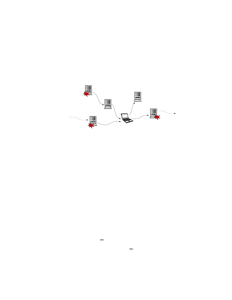
CHAPTER 5.

RESPONSE USING DYNAMIC PROGRAMMING

seek to co-operate and share the inspection outcomes. Under this scheme, an inspection

outcome at one machine is transmitted to another co-operating peer chosen randomly. The

controller on the randomly chosen machine uses such received messages to select the optimal

control to apply locally. This has the effect of a machine randomly polling several neighbors

to know the state of the environment and gives the uninfected machines an opportunity to

take appropriate actions to prevent being infected.

PSfrag replacements

, u

Chain 1

Chain 2

Figure 5.1: Alert Sharing Protocol. The laptop is our machine of interest. It uses informa-
tion, z

and z

, from different chains to choose, actions, u

and u

. It may or may not have

seen an anomaly while the machines shown with a blast have seen an anomaly.

Goal:

Now, the problem is to determine the policy that minimizes the total expected cost

over N steps, stages or time periods. Since, we solve the formulation offline, N is really not

a constraint unless it is too big. Even N = 10 could be easily solved even on a current PC

if not by hand. However, once we have the formulation, we can also solve it approximately

or analytically for larger N s. The rest of this section shows the formulation of this problem

and a solution for N = 3 and later present and discuss computer generated results for larger

N s.

5.4.2

Problem Formulation

We can see that the above description of the problem fits the general framework of

section 5.3, “Problems with imperfect state information.” The state space of the machine

consists of the two states P and P ,

State Space of the machine = {P, P } = Uninfected, Infected,

the control space consists of the two actions C and S,

Control Space = {C, S} = Continue, Stop,

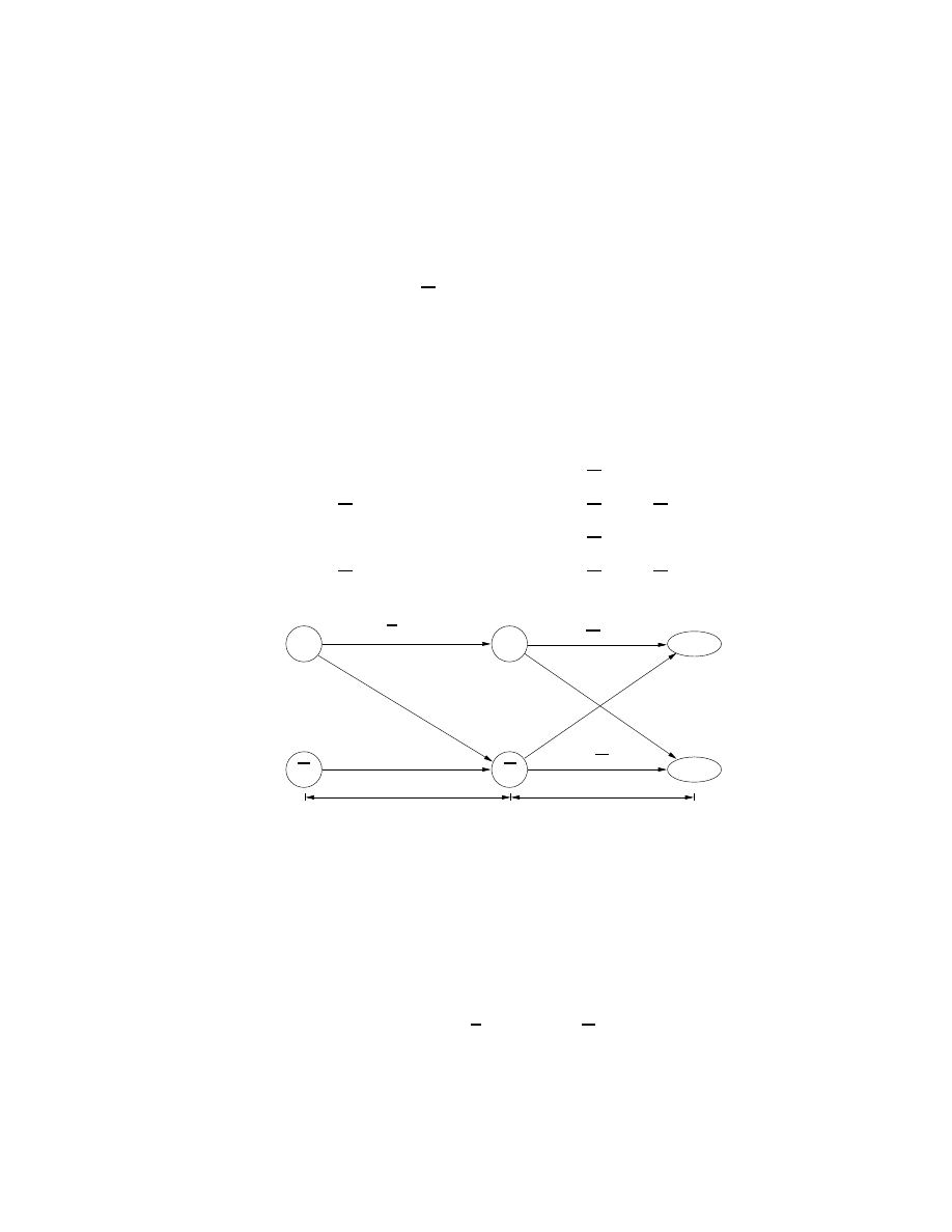
CHAPTER 5.

RESPONSE USING DYNAMIC PROGRAMMING

and the observation space consists of two elements G and B,

Observation Space = {G, B}

The machine by itself does not transit from one state to another. Left to itself, it remains

put. It is transferred from P to P only by a worm infection which is purely, a random

process; an already infected victim chooses this machine randomly. Referring back to equa-

tion (5.1), the evolution of this system depends on the current state of the system, x

the random disturbance, w

, the control, u

, and λ which is a function of the number of

machines infected on the Internet – the infectious force. Rolling the disturbance, w

, into

, the evolution of this system shown in Fig. 5.2 can be described by:

P (x

= P | x

= P, u

= C) = (1 − λ) P (x

= P | x

= P, u

= C) = λ

P (x

= P | x

= P , u

= C) = 0

P (x

= P | x

= P , u

= C) = 1

P (x

= P | x

= P, u

= S) = 1

P (x

= P | x

= P, u

= S) = 0

P (x

= P | x

= P , u

= S) = 0

P (x

= P | x

= P , u

= S) = 1

(5.11)

PSfrag replacements

C/λ

C/λ, S/1

C, S/1

State Transition

Inspection

Figure 5.2: State Transition probabilities for each action and observation probabilities for
each state.

We denote by x

, x

, . . . , x

, the states of the machine when the first, second and

the N

messages are received respectively. u

, . . . , u

denote the actions taken by the

controller upon receipt of the first . . . N

messages. Assuming the machine initially starts

in state P , the probability distribution of x

P (x

= P ) = λ,

P (x

= P ) = λ.

(5.12)

We do not have to know the initial state the machine starts as mentioned in Sec. 5.2.

This assumption is for exposition only. Note that the outcome of each inspection of the

CHAPTER 5.

RESPONSE USING DYNAMIC PROGRAMMING

machine is an imperfect observation about the state of the system. Here again, we roll in the

observation disturbance, v

, into the observation, z

. Referring back to equation (5.4), we

can view each measurement of the system state as a random variable with the probability

distribution:

P (z

= G | x

= P ) = fn

P (z

= B | x

= P ) = (1 − fn)

P (z

= G | x

= P ) = (1 − fp)

P (z

= B | x

= P ) = fp

(5.13)

where fp and fn are properties of the sensors denoting the false positive and false negative

(miss) rates.

The costs resulting from a sequence of states x

, x

, . . . , x

and controls u

, u

. . . , u

, u

) + g

, u

) + · · · + g

−1

, u

−1

) + g

)

where

g(P, C) = 0,

g(P, S) = g(P , S) = τ

g(P , C) = τ

g(x

) = 0.

(5.14)

Assuming the cost function remains the same regardless of the cardinality of the message

being processed, the sub-script k can be dropped from g. Also, g

) = 0 because u

chosen with accurate knowledge of the environment, (i.e) whether there is a worm or not.

If there is a worm, u

= S, and u

= C otherwise. The information vectors at the receipt

of each message is the same as eq.(5.5).

Note that the progression, x

, . . . , x

appears on a sequence of machines and

, . . . , u

appears on one machine. We remind readers that z

is the observed state of

the last machine in the k

chain that runs through the machine in question(the laptop in

Fig.5.1). Whereas u

is the control applied in response to z

in this machine. Our problem

now is to find functions µ

) that minimize the total expected cost

(

g(x

) +

−1

g x

, µ

)

We now apply the DP algorithm from equation (5.9). It involves finding the minimum cost

CHAPTER 5.

RESPONSE USING DYNAMIC PROGRAMMING

over the two possible actions, C and S, and it has the form

) = min

{C,S}

P (x

= P | I

, C) · g(P, C) + P (x

= P | I

, C) · g(P , C)

+ E

k+1

, C, z

) | I

, C

P (x

= P | I

, S) · g(P, S) + P (x

= P | I

, S) · g(P , S)

+ E

k+1

, S, z

) | I

, S

(5.15)

where k = 0, 1, . . . N − 1 and the terminal condition is J

) = 0. Applying the costs

given above in equations (5.14), and noticing that P (x

= P | I

, S) + P (x

= P | I

, S) is

the sum of probabilities of all elements in a set of exhaustive events which is 1, we get

) = min

· P (x

= P | I

, C) + E

k+1

, C, z

) | I

, C

+ E

k+1

, S, z

) | I

, S

, (5.16)

which is the required DP formulation of response to worms. Next, we demonstrate a solution

derivation to this formulation assuming N = 3.

5.4.3

Solution

Here we show a solution assuming that we expect to know with certainty about

the presence of a worm at the receipt of the third message, that is, N = 3. As mentioned

before, the same procedure can be followed for larger N s without loss of generality.

With that assumption, control u

can be determined precisely. If the third message

says there is a worm, we set u

= S, and we set it to C otherwise. This also means that

the cost to go at that stage is

) = 0.

(Terminal Condition)

Penultimate Stage:

In this stage we want to determine the cost J

). We use equation

(5.16) to compute this cost for each of the eight possible values of I

= (z

, z

, u

) under

each possible control, u

= {C, S}. Then, the control with the smallest cost is chosen as the

optimal one to apply for each z

. Applying the terminal condition to the DP formulation

CHAPTER 5.

RESPONSE USING DYNAMIC PROGRAMMING

(5.16), we get

) = min

· P (x

= P | I

, C) + E

, C, z

) | I

, C

+ E

, S, z

) | I

, S

= min

· P (x

= P | I

, C) + E

) | I

, C

, τ

+ E

) | I

, S

. . . From eq (5.6)

= min

· P (x

= P | I

, C) + E

{0} , τ

+ E

{0}

. . . Terminal Condition

= min

· P (x

= P | I

, C) , τ

The probabilities P (x

= P | I

, C) can be computed using Bayes’ rule and

eqs.(5.11–5.13) assuming the machine starts in state P . We show the calculations for a

couple of them here. See Tables 5.1 & 5.2 for complete sample solutions.

(1) P (x

= P | G, G, S)

P (x

= P , G, G, | S)

P (G, G, | S)

={P,P }

P (G|x

= i) · P (x

= i) · P (G|x

= P ) · P (x

= P |x

= i, u

= S)

={P,P }

P (G|x

= i) · P (x

= i) · P (G|x

= j) · P (x

= j|x

= i, u

= S)

(fp · λ · fn · 0) + (fn · λ · fn · 1)

(fp · λ · fp · 1) + (fp · λ · fn · 0) + (fn · λ · fp · 0) + (fn · λ · fn · 1)

(2) P (x

= P | G, G, C)

P (x

= P , G, G, | C)

P (G, G, | C)

={P,P }

P (G|x

= i) · P (x

= i) · P (G|x

= P ) · P (x

= P |x

= i, u

= C)

={P,P }

P (G|x

= i) · P (x

= i) · P (G|x

= j) · P (x

= j|x

= i, u

= C)

(fp · λ · fn · λ) + (fn · λ · fn · 1)

(fp · λ · λ · 1) + (fp · λ · fn · λ) + (fn · λ · fp · 0) + (fn · λ · fn · 1)

CHAPTER 5.

RESPONSE USING DYNAMIC PROGRAMMING

In general, we have

P (x

) =

P (x

· I

)

P (I

)

P (I

) =

={P,P }

· · ·

={P,P }

P (z

)P (x

) ·

P (z

)P (x

−1

, u

−1

)

P (x

· I

) = P (I

−1

) · P (z

)P (x

−1

, u

−1

)

The cost-to-go, J

), thus calculated are used for the zeroth stage.

Stage

In this stage we want to determine the cost J

). We use equation (5.16) and

values of J

) calculated during the previous stage to compute this cost. As before this

cost is computed for each of the two possible values of I

= (z

) = {G, B}, under each

possible control, u

= {C, S}. Then, the control with the smallest cost is chosen as the

optimal action to perform for the observed state of the machine. Thus we have,

) = min

· P (x

= P | I

, C) + E

) | I

, C

, τ

+ E

) | I

, S

The optimal cost for the entire operation is finally given by

∗

= P (G)J

(G) + P (B)J

(B)

We implemented a program that can solve the above formulation for various values

of λ, fp, & fn. We ran the program and tabulated the resulting rule-set in tables 5.1 &

5.2. The next section gives a brief discussion on choosing realistic values for the various

parameters, presents and discusses the results from our program runs.

5.5

Alternate Re-formulation using Sufficient Statistics

In section 5.3.2, we presented a re-formulation of the imperfect state information

problem in which the information vector, I

, assumed the state of the system and included

all the observations made and controls applied so far. This increases the dimension of I

by two for each transition of the system after the first one, exploding the state space that

needs to be explored.

In this section, we will present the essence of an alternative re-formulation where

the state of the system is probabilistically represented conditioned only on the latest obser-

vation and control applied. In other words, we reduce I

to smaller dimensions containing

CHAPTER 5.

RESPONSE USING DYNAMIC PROGRAMMING

only the Sufficient Statistics yet summarizing all essential contents of I

as far as control is

concerned. We first explain these two terms before presenting the re-formulation itself.

5.5.1

Sufficient Statistic

Refer back to eqs. (5.8) and (5.9). Suppose we can find some function S

) such

that the minimizing control in those two equations depends on I

through S

). Then,

the right hand side of those two equations can be written as:

min

), u

Such a function S

is called a Sufficient Statistic. An optimal policy obtained by the above

minimization can be written as

∗

) = µ

)

where µ

is an appropriate function. Thus, if S

) is characterized by a set of fewer

numbers than I

, it may be easier to implement the policy in the form u

= µ

)

and take advantage of the data reduction.

5.5.2

Conditional State Distribution

A Couple of candidates for S

are:

1. The identity function, S

) = I

2. The conditional probability distribution, P

, of the state given the information

vector. This is also known as the belief state of the system.

It is assumed here that v

depends explicitly only on the immediately preceding state,

control and the system disturbance and not on any of the earlier ones. Under this assump-

tion, we state without proof that

J(I

) = J

(5.17)

k+1

= Φ

, u

, z

)

(5.18)

where J

is an appropriate function, and Φ

is a function that can be determined from the

problem. We refer the readers to Bertsekas [22] for the proof and justification of eqs. (5.17)

and (5.18) respectively.

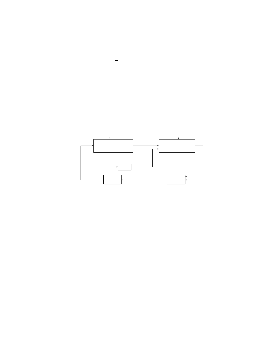
CHAPTER 5.

RESPONSE USING DYNAMIC PROGRAMMING

Given that P

is a sufficient statistic function, we have,

) = µ

k = 0, 1, . . . , N − 1,

Regardless of the computational reduction, this representation of the optimal policy as a

sequence of functions of P

, is conceptually useful. It provides a decomposition of the

optimal controller into two parts:

(a) An estimator, which generates P

using only the most recent observation and

control, z

and u

−1

(b) An actuator, which generates u

based on P

Actuator

System

Measurement

Delay

Estimator

PSfrag replacements

= f

, u

, w

)

= h

, u

−1

, v

)

−1

Figure 5.3: The controller split into an Estimator and an Actuator

Fig. 5.3 explains this concept. We also learn from the figure that, the imper-

fect state information problem has now been reduced to a perfect belief state information

problem. Here, the system state is P

that evolves according to Φ

while the controller

controls the probabilistic state P

so as to minimize the expected cost-to-go conditioned

on the information I

available. This split gives a better handle on the design of these two

distinct aspects of the controller.

5.5.3

Reduction using Sufficient Statistics

Armed with the above eqs. (5.17) and (5.18), we can now re-state the DP algorithm

(5.8) & (5.9) as:

−1

N −1

) = min

N −1

−1

, u

−1

, w

−1

)

+ g

−1

, u

−1

, w

−1

)|I

−1

, u

−1

(5.19)

CHAPTER 5.

RESPONSE USING DYNAMIC PROGRAMMING

for k = N − 1 and for k < N − 1,

) = min

k+1

, u

, w

) + J

, u

, z

)

, u

(5.20)

Finite State Systems.

Suppose that the system under study is a finite state system

such that x

= {1, 2, . . . , n} and that when a control u is applied the system goes from

state i to state j with a probability of p

(u). For each state x

the system assumes (which

is hidden), and a control u

applied, a cost of g

, u

) is incurred. The terminal cost for

being in state x

at the end of N stages is denoted by G

). We want to minimize the

expected sum of costs incurred over the N stages. This problem can be reformulated into

a perfect state information problem where the objective is to control the column vector of

conditional probabilities:











n
k











where

i
k

= P (x

= i|I

i = 1, . . . , n

is called the belief state and evolves according to eq. (5.18), where Φ represents an

estimator. p

is given or can be calculated from the problem data. The corresponding DP

algorithm (eqs.(5.20) & (5.19)) has the form:

) = min

g(u

) + E

k+1

, u

, z

)

, u

(5.21)

) = p

(5.22)

where g(u

) is the column vector with components g(1, u

), . . . , g(n, u

). p

g(u

), the ex-

pected stage cost, is the inner product of the vectors p

and g(u

5.5.4

Response Formulation using Sufficient Statistics

The worm response problem as we have described in section 5.4.1 is a finite state

system and can be solved using the last DP algorithm, (5.21) & (5.22), mentioned above with

appropriate re-formulation. The only parameters that we need to define are the conditional

probability distribution of the state, P

, and the corresponding evolution function Φ

Once these parameters are defined, it is straightforward to compute the minimizing costs

and corresponding actions.

CHAPTER 5.

RESPONSE USING DYNAMIC PROGRAMMING

We show one such solution assuming, again, that N = 2. We define the conditional

state distribution and their evolution as:

P (x

= P |I

)

P (x

= P |I

)

and

= Φ

, u

, z

) =











fn+(1−p

)fp

if u

= S,

= G,

fn+(1−p

)fp

if u

= S,

= B,

fn+(1−p

)λ fn

fn+(1−p

)(λ fp+λ fn)

if u

= C,

= G,

fn+(1−p

)λ fn

fn+(1−p

)(λ fp+λ fn)

if u

= C,

= B

(5.23)

based on the problem data and Fig. 5.2. We define only the probability of the machine

being infected because the state space of the system is binary. P (x

= P |I

) automatically

implies P (x

= P |I

). This makes the presentation simpler. Note that the belief state, p

is a column vector with only one element. This makes the cost vectors also column vectors

with only one element.

g(C) =

g(P , C) = τ

g(S) =

g(P , S) = τ

We will show how one of these p

is derived. The rest are derived similarly. For example,

= P (x

= P |u

= C, z

= G) =

P (x

= P , z

= G|u

= C)

P (z

= G|u

= C)

fn + (1 − p

)λ fn

(1 · fn + 0 · fp) + (1 − p

)(λ · fp + λ · fn)

Substituting these definitions into the DP re-formulation above, (eqs. 5.21 & 5.22), the

solution we need is:

) = 0,

) = min[τ

· p

, τ

)

= min

· p

+ P (z

= G|p

, C)J

, C, G)

+ P (z

= B|p

, C)J

, C, B)

+ P (z

= G|p

, S)J

, S, G)

+ P (z

= B|p

, S)J

, S, B)

We spare the reader of tedious calculations but mention that the numerical solution to

this set of equations, though same, is much easier to compute than that presented for the

previous (sec. 5.4.3) re-formulation.

CHAPTER 5.

RESPONSE USING DYNAMIC PROGRAMMING

5.6

A Practical Application

5.6.1

Optimal Policy

Table 5.1 shows the optimal policies for a few different values of λ. In the first two

scenarios for high λ, the policy chooses S for a B observation and C for a G observation.

An interesting policy arises in the last scenario. It says, with a low λ the best policy is S

only when there are two consecutive B observations. This table only demonstrates a sanity

check of the algorithm as the machine will not know the current value of λ and hence cannot

meaningfully choose the policy to implement.

However, we do know the costs payable in the event of infection. Table 5.2 shows

the optimal policies for a few different costs of infection, τ

. In the first scenario where

the cost of operating a infected is not much higher than stopping the machine, the optimal

policy is S when you get a B observation and C otherwise. This enables us to back-off

from the response when we see a G. In the second scenario, where τ

= 10 · τ

, the optimal

policy is to S upon a B and remain there. The policy for the last scenario is quite drastic

in keeping with the huge τ

. It chooses S the first time we get any message. Even if that

message is a G because the fact that an inspection was triggered means that something

abnormal has happened and the outcome could be a false negative. This policy chooses C

only when we see two G messages consecutively.

5.6.2

Choosing λ

Choosing realistic values for the various parameters is of great importance if the

solution needs to be of any practical value. Here we discuss some factors that need to be

considered while choosing the parameters’ values for building the rule-sets.

The value of λ varies with the extent of infection in the Internet. Given that we

are still uncertain whether there is a worm or not in the Internet, λ can not be determined

with any accuracy or certainty. Rather, only estimates can be made.

So, we again use the distributed Sequential Hypothesis Testing developed ear-

lier to estimate λ [34]. Given a sequence of observations ~y = {y

, y

, . . . , y

}, made by

the other participating nodes and two contradicting hypotheses that there is a worm on the

Notice that some of the I

such as (B, B, C) may not be reachable because of the control policy applied

in stage 0.

CHAPTER 5.

RESPONSE USING DYNAMIC PROGRAMMING

Internet(H

) and not(H

), the former is chosen when the likelihood ratio of these hypotheses

is greater than a certain threshold η [34]. This threshold η is determined by the perfor-

mance conditions required of the algorithm. Assuming the observations are independent,

the likelihood ratio of these two hypotheses and η are defined as follows:

L(~y) =

P (y

)

P (y

)

η =

(5.24)

where DD is the minimum desired detection rate and DF is the maximum tolerable false

positive rate of the distributed Sequential Hypothesis Testing(dSHT) algorithm. We define

each of the above probabilities as follows:

P (y

= B | H

) = [λ (1 − fn) + (1 − λ) fp]

P (y

= G | H

) = [(λ fn) + (1 − λ)(1 − fp)]

P (y

= B | H

) = fp

P (y

= G | H

) = (1 − fp)

(5.25)

The first one of those above is the probability of a B observation is the sum of probability

of getting infected (λ) times the probability of detection and the probability of not getting

infected((1 − λ)) times the probability of false positives. The others are defined similarly.

For any given sequence of observations, we calculate L(~y) for several λ values –

say for ten different values in steps of 0.1 starting at 0.1. The minimum λ for which the

L(~y) exceeds η will be taken as the current levels of infection and used appropriately in

calculating the optimal responses.

Given equations (5.24) and (5.25), all observations over a sequence of nodes can

be expressed as one number, the L(~y). A node receiving this number from a neighbor, can

update it using its own observations and eq. (5.24) and the corresponding λ picked for

applying the DP algorithms to choose response.

In practice however, a table of rule-sets would be calculated offline for each value of

λ. Then, the table corresponding to the λ chosen as above will be consulted for the optimal

action to take given the observation vector received and the sequence of local observations

and actions taken so far locally.

Thus, each node only receives a likelihood ratio of the worm’s presence from its

peers. Each node also has to only remember its own past observations and corresponding

actions.

CHAPTER 5.

RESPONSE USING DYNAMIC PROGRAMMING

5.6.3

Larger N s

Using the Sufficient Statistics re-formulation developed in section 5.5, it becomes

easy to apply the model for larger N s. We implement this model and evaluate it in a

simulation. This evaluation and the results are discussed in the next section.

5.7

Evaluation

The sufficient statistics formulation discussed in the previous section was imple-

mented and evaluated with a discrete event simulation. The simulation consisted of 1000

participants with 10% of the machines being vulnerable. We set the number of stages to

operate the machine, N = 4 to calculate the rule-sets. Note that N = 4 is used only to

calculate the rule-sets but the machines can be operated for any number of steps. N is

essentially the number of past observations and actions that each machine remembers. The

local IDSes were set to have a false positive and false negative rates of 0.1. These charac-

teristics of the local IDS is used to calculate the probability of infection, λ with a desired

worm detection rate of 0.9 and failure rate of 0.1. In all the following experiments, we used

a random scanning worm which scans for vulnerable machines once every unit-time.

5.7.1

Experiments

Parameters of Evaluation:

We conducted experiments to evaluate the effectiveness of

the response model discussed here. We designed a set of experiments to verify the efficacy

of the model and to understand the effect of various parameters on the effectiveness of the

model in controlling the spread of the worm. The only free variable we have here is the ratio

of the costs of stopping the service to that of getting infected. There is no one particular

parameter that can measure or describe the effectiveness of the response model. Rather,

the effectiveness is described by a pair of parameters. These parameters are:

• Number of machines that are not infected.

• Number of machines that provide service, i. e. in state C.

So, in this evaluation, we will measure the effect of various τ

/τ

ratios on above two

parameters.

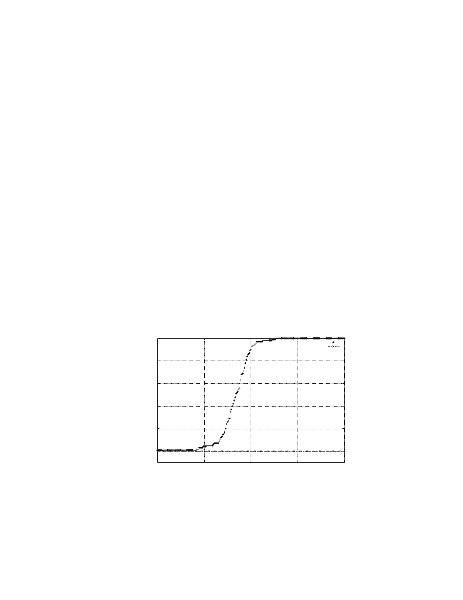
CHAPTER 5.

RESPONSE USING DYNAMIC PROGRAMMING

Algorithm:

The evaluation was conducted as a discrete-event simulation. The algorithm

for the simulation is as follows. At each time cycle,

• all infected machines attempt one infection,

• all machines that had a alert to share, share the likelihood ratio that there is a worm

on the Internet with one another randomly chosen vulnerable node,

• and all vulnerable machines that received an alert earlier take a response action based

on the information received and the current local observations.

Results:

In the first experiment, we want to make sure that we have a worm that behaves

as normal random scanning worm and validate the response model for degenerate cases. We

verify this by providing no response. This response can be achieved by setting the cost ratio

to 1. This means that the cost of stopping the service is the same as getting infected. In

this scenario, we expect the response model not to take any defensive measures against

suspected infection attempts. As expected, we see in Fig. 5.4, that none of the machines

are stopped (S state). The worm spreads as it would spread when there is no response

model in place. This validates our worm and also our response model.

100

150

200

# of hosts

Time(no units)

Spread of a worm with no response - infected : blocked cost :: 1 : 1

Infected
Blocked

Figure 5.4: No machines are stopped when the cost of being infected is the same as cost of
shutting down the machine.

As another sanity check we set the machines to remember infection attempts for-

ever. Under this policy, once a machine enters the S state, it remains in that state forever.

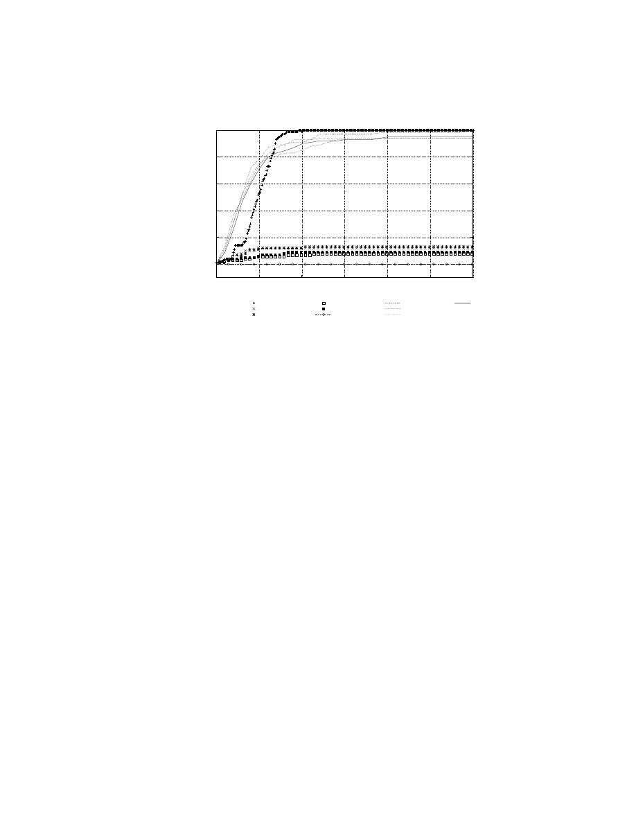
CHAPTER 5.

RESPONSE USING DYNAMIC PROGRAMMING

100

150

200

250

300

# of hosts

Time(no units)

System behaviour for various ratios of infected : blocked costs

(Infected) 1

3
5

30
50

(Blocked) 1

3
5

Figure 5.5: Once entered the S state, a machine stays there.

We see that in this case (Fig. 5.5) the number of machines infected are very low except

when τ

/τ

= 1.

In the next experiment, we try to understand the behavior of our response model

in various situations. Since the only free variable is the ratio τ

/τ

, we repeat the previous

experiment with various values for that ratio. The results for this set of experiments is

shown in Fig. 5.6. This graph shows behavior of our response model in five different tests.

There are two different curves for each test indicating the number of vulnerable machines

being infected and the number in S state against time. We can see that when the ratio is 1,

the number machines that are in S state is 0. As the ratio τ

/τ

rises, the response becomes

stricter. We see that the number of machines in the stopped(S) state is higher when the

cost of being infected is higher and correspondingly the worms spreads significantly slower

than without any response in place.

5.7.2

Effects of increasing N

The experiments shown earlier in this section were all conducted with N = 4. An

interesting question to ask here, “What happens if we increase the value of N ?”. Fig. 5.7

shows the performance of the system for various values of N while holding the ratio of

/τ

constant at 30. The set of sigmoidal curves trace the growth of the worm, while the

other set of curves trace the number of nodes that are shut-down at any given instance of

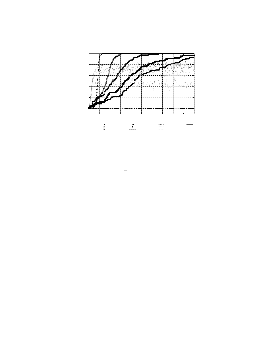
CHAPTER 5.

RESPONSE USING DYNAMIC PROGRAMMING

100

200

300

400

500

600

700

800

900

1000

# of hosts

Time(no units)

System behaviour for various ratios of infected : blocked costs

(Infected) 1

3
5

30
50

(Blocked) 1

3
5

Figure 5.6: Higher costs of being infection invoke stricter responses.

time. We notice that there is no appreciable slowing of the worm with increased values of

N – all the worm growth curves are bunched up together. This is due to the small number

of dimensions to the state – x

∈ {P, P } – a larger observation space does not contribute

much to improve the performance of the system. Note that the x-axis is in log-scale in this

figure.

5.8

Limitations and Future Work

There are several topics in this chapter left to be addressed in the future. There

are issues to be addressed at three different levels – in the model itself, in the evaluation of

the model and problem that would arise during the practical implementation of this model.

This is a collaborative response model. As with any collaborative effort, there

is a host of issues such as privacy, confidentiality, non-repudiation, etc, that will need to

be addressed during practical adoption. Thankfully, these are issues for which there are

solutions available already through cryptography and Ipsec. Still, co-operation amongst

various entities on the Internet such as amongst corporate networks pose more legal and

economic problems than technical. In such cases where sharing anomaly information with

networks outside of the corporation is not feasible, applying this response model within the

corporate network itself can provide valuable protection.

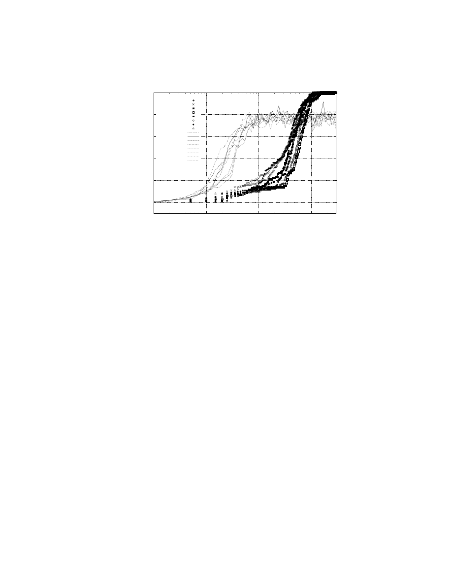
CHAPTER 5.

RESPONSE USING DYNAMIC PROGRAMMING

100

1000

# of hosts

Time(no units, Log scale)

System behaviour for various N

Various N’s

(Infected) 3

4
5
6
7
8
9

(Blocked) 3

4
5
6
7
8
9

Figure 5.7: Larger N s do not contribute much to improve performance.

When there is a cost to sampling packets, this model can be extended to optimally

stop the sampling process and declare either that there is a worm or that there is no worm.

Interestingly, this extension would lead us to the distributed Sequential Hypothesis Testing

that we discussed in the previous chapter. Actions such as C and S if applied frequently

could lead to a very unstable system. We need to evaluate this factor in light of ambient

anomaly levels in different environments. This is a problem that arises during adoption of

this technology. However, this can be addressed in various ways. For example, the set of

response options can be made slightly larger with options to have several levels of reduced

functionality instead completely shutting down the service.

One of the major problems that needs to be addressed while implementing this

model in reality is the assignment of realistic values to the costs τ

and τ

. However, there

is some prior work that attempts to assign costs to various responses that can used [18, 76].

As already argued at length in chapter 3, evaluating worm defenses is a difficult

problem. At one extreme we have realistic evaluation possible only on the Internet but is

infeasible. At the other extreme, we have mathematical models only. In between these two

extremes, we have simulations such as the one used in this chapter and emulations such as

the one used in the previous chapter 4.

With the availability of data about Internet traffic during worm outbreaks, it may

be possible to evaluate the defense model on a network testbed such as Emulab by replaying

CHAPTER 5.

RESPONSE USING DYNAMIC PROGRAMMING

the traffic for a scaled down version of the Internet. Such an experiment would need the

available data to be carefully replayed with tools such as TCP Replay,TCP Opera, etc.

This is a task that can explored in the future to evaluate worm defenses. Scaling down the

Internet is another problem in itself [117].

An issue still left to be explored is the behaviour of this model in face of false

alarms and isolated intrusions. For eg., consider one and only participant raising an alarm

for an isolated event and several other participants choosing the S control. We would like to

know when these participants would apply the C control. Trivially, we can set a time-out

for the defense to be turned-off. However, the time-out should be chosen carefully and

probably be dynamic to guard against exposing oneself to slow worm attacks.

CHAPTER 5.

RESPONSE USING DYNAMIC PROGRAMMING

λ = 0.50, fp = 0.20, fn = 0.10, τ

= 1, τ

= 2

Information vector

Optimal Cost-to-go

Optimal Action

Stage 1

(G, G, S)

0.031

(B, G, S)

0.720

(G, B, S)

0.720

(B, B, S)

1.000

(G, G, C)

0.270

(B, G, C)

1.000

(G, B, C)

1.000

(B, B, C)

1.000

Stage 0

(G)

0.922

(B)

1.936

Start

1.480

λ = 0.30, fp = 0.20, fn = 0.10, τ

= 1, τ

= 2

Information vector

Optimal Cost-to-go

Optimal Action

Stage 1

(G, G, S)

0.013

(B, G, S)

0.388

(G, B, S)

0.388

(B, B, S)

1.000

(G, G, C)

0.119

(B, G, C)

0.569

(G, B, C)

1.000

(B, B, C)

1.000

Stage 0

(G)

0.604

(B)

1.793

Start

1.091

λ = 0.10, fp = 0.20, fn = 0.10, τ

= 1, τ

= 2

Information vector

Optimal Cost-to-go

Optimal Action

Stage 1

(G, G, S)

0.003

(B, G, S)

0.118

(G, B, S)

0.118

(B, B, S)

1.000

(G, G, C)

0.031

(B, G, C)

0.154

(G, B, C)

0.726

(B, B, C)

1.000

Stage 0

(G)

0.252

(B)

1.227

Start

0.515

Table 5.1: An optimal policy table - varying λ

CHAPTER 5.

RESPONSE USING DYNAMIC PROGRAMMING

λ = 0.30, fp = 0.20, fn = 0.10, τ

= 1, τ

= 2

Information vector

Optimal Cost-to-go

Optimal Action

Stage 1

(G, G, S)

0.013

(B, G, S)

0.388

(G, B, S)

0.388

(B, B, S)

1.000

(G, G, C)

0.119

(B, G, C)

0.569

(G, B, C)

1.000

(B, B, C)

1.000

Stage 0

(G)

0.604

(B)

1.793

Start

1.091

λ = 0.30, fp = 0.20, fn = 0.10, τ

= 1, τ

= 10

Information vector

Optimal Cost-to-go

Optimal Action

Stage 1

(G, G, S)

0.067

(B, G, S)

1.000

(G, B, S)

1.000

(B, B, S)

1.000

(G, G, C)

0.594

(B, G, C)

1.000

(G, B, C)

1.000

(B, B, C)

1.000

Stage 0

(G)

1.279

(B)

2.000

Start

1.575

λ = 0.30, fp = 0.20, fn = 0.10, τ

= 1, τ

= 100

Information vector

Optimal Cost-to-go

Optimal Action

Stage 1

(G, G, S)

0.665

(B, G, S)

1.000

(G, B, S)

1.000

(B, B, S)

1.000

(G, G, C)

1.000

(B, G, C)

1.000

(G, B, C)

1.000

(B, B, C)

1.000

Stage 0

(G)

1.744

(B)

2.000

Start

1.849

Table 5.2: An optimal policy table for various costs of infection, τ

CHAPTER 6.

CONCLUSION

Chapter 6

Conclusion

This chapter recollects what has been detailed in the previous chapters and elicits

a holistic view of worm defense from what has been presented. It also identifies some of the

critical problems still unsolved that are significant impediments to progress in the field and

suggests future directions for research in the field.

6.1

Summary

This dissertation gave a thorough overview of the history of worms and worm

research, examples of worms seen in the wild, and of the hypothetical variety. It also

identified the various problems involved in defending against worms, and paradigms used

in addressing them.

As already observed in chapter 2, detection and response form two of the three

fundamental blocks of a strong worm defense program, prevention being the third one. The

first two are reactive measures (i. e.) those aspects of defense that need to work while a

worm has already been launched and is spreading currently. The third one is a proactive

measure . This dissertation addressed the two most important components – detection and

response – the reactive aspects of worm defense.

Deviating from the currently popular paradigm of handling worms by automatic

signature generation and pattern matching, the techniques developed in this dissertation are

independent of worm signatures. This deviation helps to counter polymorphic and zero-day

worms effectively.

Worms, by definition, are a distributed phenomenon. Hence, the detection tech-

CHAPTER 6.

CONCLUSION

nique developed here uses observations and evidence from various sites instead of focusing

on one particular machine or network. It is a distributed and decentralized detection tech-

nique, and hence does not suffer from single point failures as some of the other popular

techniques do.

This detection technique used dSHT to build a strong worm detector using weak

or imperfect anomaly detectors as components. The performance characteristics of this

strong worm detector thus built can be tuned to the desired rates of successful detection

and misses.

The distributed nature of this technique and its ability to build strong detectors

out of weak components helps tap the vast amounts of anomaly information available at

end-user systems – home and office users primarily. These are users who cannot or usually

do not run sophisticated intrusion detectors but are still targets of worm attacks. The poor

anomaly or intrusion detectors that they run cannot make authoritative detections of worms

but by co-operating with each other, they can detect worms in unison with high degree of

accuracy.

Response techniques developed hitherto by the research community address the

worm problem after detecting the worm. Hence, they primarily deal with automatic patch

and signature generation, distribution, and application. However, it is clear that this strat-

egy of catching up is not very effective. Much damage can be done by the worm before the

patches are disseminated to all susceptible machines. In contrast, the strategy developed

here deals with responding to events that are possibly due to a worm but cannot be verified

yet.

This technique is applicable while the detection process is still in progress – during

the time when reasons for the observed anomalies are unknown. During such instances,

drastic responses such as shutting down services need to considered carefully before being

applied. While such response during a real worm attack is desired even if it results in loss

of service, they are costly actions to undertake in response to false alarms or when there

is no danger of a worm attack. On the other hand, not responding to suspicious events

can be very expensive when those events were really due to a worm. The response model

developed here considers these various alternatives, evaluates the costs of each action and

inaction, and chooses the option that would result in an optimal long-term cost. If and

when evidence suggests that the observed anomalies are not due to a worm, the system

automatically backs-off from the response actions activated. Hence, the response system is

CHAPTER 6.

CONCLUSION

dynamic, adjusting to the current environment. The response technique here uses a novel

control-theoretic approach using Dynamic-Programming tools.

Though the response system is itself dynamic, the dynamic programming algo-

rithm does not have to be solved in real-time. The algorithm is pre-computed off-line and a

control rule-set is generated that can be easily looked up for appropriate responses to imple-

ment for each observation of the environment. Moreover, individual nodes are free to choose

appropriate response actions and are not constrained by a central leader or controller. Thus

the response is completely localized.

No assumptions are made about the topology of the network to which these co-

operating peers are attached for either of the above algorithms to work. All that is required

is network connectivity and an ability to reach the peers. Thus, these algorithms work

regardless of the scanning algorithm employed by a worm. However, detection could be

delayed and responses may be ineffective if the worm is a sub-net scanning worm whereas

the co-operating peers are assumed to be distributed randomly all over the Internet and

the algorithms choose their peers at random from a given set to exchange information.

In addition to these two important techniques, this dissertation also developed

an evaluation framework to evaluate such new technologies. As an example it showed

how a Hierarchical Model of Defense that was developed earlier can by evaluated by this

framework.

Thus, by addressing detection, response and mitigation aspects of worm defense

and by developing an evaluation framework, this dissertation provides an end-to-end solu-

tion to the worm problem.

6.2

Future Directions

There are several aspects to the proposed solutions that still need to be addressed.

For example, the evaluation framework presented in chapter 3 still suffers from scale-down

issues. Coming up with a solution to this problem will unlock a great deal of understanding

about the dynamics of Internet-wide, large scale phenomenon such as computer worms,

distributed denial-of-service, etc. This situation arises from a more fundamental problem –

the complete topology of the Internet is unknown. So, a study mapping the topology of the

Scale-down is a problem of too small a statistical sample involved in the experimental setup compared

to the real Internet.

CHAPTER 6.

CONCLUSION

Internet will be very useful; this can be then scaled-down with scaling hypothesis proposed

by Psounis et al. [91].

The experiments conducted and described in this dissertation were done on the

Emulab testbed without any background traffic. Replicating the huge volumes of traffic

seen on the Internet is infeasible and in fact, not even required. One possible approach is to

have a few nodes of the testbed generate the subset of traffic from the Internet that would

be pertinent to the experiment being conducted. The volume of such traffic would be more

manageable. For example, imagine an experiment modeling an enterprise network. There

is no need to generate the ambient Internet traffic associated with a military domain or

even the traffic within another network that is not visible to this enterprise network. It is

sufficient to generate traffic that would normally be seen by the enterprise domain that is

being modeled.

A faithful means of reproducing ambient traffic as would be seen on the Internet

would be a great help in conducting controlled experiments that reflect the reality. So

far, we do not have any solution to fill this gap. There are tools such as tcpreplay and

tcpopera

, etc, that can play back recorded traffic. However, there is no clear understanding

on how to model the traffic such that it can be generated from a specification rather than

just by replaying pre-recorded traffic.

We do not yet know what are necessary and sufficient descriptions of an anomaly.

This is a huge gray-area. Anomaly detection has always been plagued by huge amounts of

false-positives. A sizable reduction in the false positive rates is highly desired. Specification-

based anomaly detection is one way to go about it.

The next concern in these distributed algorithms is the privacy concern about

sharing anomaly information with other peers. A provably secure data sanitization process

will be a great selling point for these systems. Also there is a need for security and au-

thentication in the communication amongst the co-operating peers. IPSec might provide

a suitable solution. There are also certain initiatives such as CIDF [37], IDIAN [55] and

IDMEF [61] but none of them is being used currently.

A leading cause for the prevalence of worms is the homogeneity of computer

systems, particularly computer with pre-installed commercial applications and operating

systems. These systems invariably ship operating systems compiled with the same con-

figurations. An attacker who can remotely exploit a vulnerability in one such machine,

immediately gains the power to attack millions of other similar machines Internet-wide.

CHAPTER 6.

CONCLUSION

So, some heterogeneity in the way commercial systems are shipped can go a long way in

frustrating the spread of worms. One means of achieving this is Address Space Layout

Randomization.

In this technique, dynamically loadable libraries are loaded on to random locations

based on a certain key on each machine rather than one preferred location across machines.

This helps to stop worms that make assumptions about the location of certain functions in

the system’s image in memory. However, smarter worms can be built to locate the required

functions by first locating the key. Stronger cryptographic solutions might help here.

6.3

Final Observations

Regardless of the various sophisticated techniques being developed for countering

worms, going by the history of the past worm attacks, simply applying patches in a timely

fashion will alleviate the problem to a great extent. The next best defense is to shut-down

unnecessary network services that are turned on by default. It is even better if these service

are shut-down by default.

The days of extremely fast worms that just create havoc without any particular

benefits to the attackers are believed to be gone. Such attackers’ population has dwindled.

The current and future attackers are in the trade after particular benefits. These benefits

include identity thefts, financial fraud and computers that can be hooked to botnets. The

final motive is financial gain. Such activities require the panning of large numbers of com-

puters without raising any suspicions. Slow spreading worms are a perfect tool to carry out

such an operation will dominate the future worm scene.

After all, computer security is not all about worms. Worms are just one small part

of the huge taxonomy of malware and other issues afflicting the reliability of computing

systems. In general, the techniques developed here can be extended to be used in other

scenarios that involve distributed phenomenon; not only worms. The detection technique

developed here can also be used to trouble-shoot network defects. Identifying problems that

can be solved using these approaches form one of the future directions of research.

BIBLIOGRAPHY

Bibliography

[1] “EMIST ESVT Software Version 2.0.”.

Internet.

http://emist.ist.psu.edu/ESVT2/

download_esvt2.html\#Overview

[2] “EMIST Project Overview”. Internet. http://www.isi.edu/deter/emist.temp.html.

[3] “EMIST Tool Suite”. Internet. http://www.cs.purdue.edu/homes/fahmy/software/emist/

index.html

[4] “HOL, http://www.cl.cam.ac.uk/Research/HVG/HOL/”. Internet.

[5] NS: Nework Simulator. Internet. http://www.isi.edu/nsnam/ns, Last Accessed: Feb 08,

2007.

[6] SNORT IDS. Internet. http://www.snort.org.

[7] “SSFNet”. Internet. http://www.ssfnet.org, Last Accessed: June 21, 2005.

[8] Code-red: a case study on the spread and victims of an internet worm. In Proceedings of the

Internet Measurement Workshop (IMW), 2002.

[9] “TrendCenter”. Internet, July 2003. http://AttackTrends.com.

[10] M. Abdelhafez and G. Riley. “Evaluation of worm containment algorithms and their effect on

legitimate traffic”. In Third IEEE International Workshop on Information Assurance (IWIA),
March 2005.

[11] John Mark Agosta, Abraham Bachrach, Denver Dash, Branislav Kveton, Alex Newman, and

Eve Schooler. Distributed inference to detect a network attack. In Proceedings of the Adaptive
and Resilient Computing Security Workshop (ARCS). Santa Fe Institute, 2005.

[12] E. A. Akkoyunlu, K. Ekanadham, and R. V. Huber. Some constraints and tradeoffs in the

design of network communications. In SOSP ’75: Proceedings of the fifth ACM Symposium
on Operating Systems Principles, pages 67–74. ACM Press, 1975.

[13] Kostas G. Anagnostakis et al. A cooperative immunization system for an untrusting internet.

In Proceedings of the 11th IEEE International Conference on Networks (ICON03), pages 403–
408, October 2003.

[14] Kostas G. Anagnostakis, Michael B. Greenwald, Sotiris Ioannidis, and Angelos D. Keromytis.

Robust reactions to potential day-zero worms through cooperation and validation. In Proceed-
ings of the 9th Information Security Conference (ISC)., 2006. To Appear.

[15] D Armstrong, S Carter, G Frazier, and T Frazier. Autonomic defense: Thwarting automated

attacks through real-time feedback control. In Proceedings of the DISCEX III, Washington,
DC, April 2003.

BIBLIOGRAPHY

[16] R. Bajcsy et al. Cyber defense technology networking and evaluation. Commun. ACM,

47(3):58–61, 2004.

[17] Robert W. Baldwin.

“Kuang:

Rule based security checking.”.

Documentation in

ftp://ftp.cert.org/pub/tools/cops/1.04/cops.104.tar. MIT, Lab for Computer Science Pro-
gramming Systems Research Group.

[18] Ivan Balepin, Sergei Maltsev, Jeff Rowe, and Karl Levitt. Using specification-based intrusion

detection for automated response. In Proceedings of the 2003 RAID, Pittsburg, 2003.

[19] Thomas Ball, Rupak Majumdar, Todd D. Millstein, and Sriram K. Rajamani. Automatic

predicate abstraction of c programs. In SIGPLAN Conference on Programming Language
Design and Implementation, pages 203–213, 2001.

[20] Thomas Ball and Sriram K. Rajamani. Automatically validating temporal safety properties

of interfaces. Lecture Notes in Computer Science, 2057:103+, 2001.

[21] Andy Bavier et al. Operating systems support for planetary-scale network services. In Pro-

ceedings of the 1st USENIX Symposium on Networked Systems Design and Implementation
(NSDI ’04), San Francisco, CA, USA, March 2004.

[22] Dimitri P. Bertsekas. Dynamic Programming and Optimal Control, volume 1. Athena Scien-

tific, third edition, 2005.

[23] B.G.Barnett. “NOOSE - Networked Object-Oriented Security Examiner”. In Proceedings of

the 14th Systems Administration Conference, USENIX Association, Nov 2000.

[24] Sandeep Bhatkar, Daniel C. DuVarney, and R. Sekar. Address obfuscation: an efficient ap-

proach to combat a broad range of memory error exploits. In 12th USENIX Security Sympo-
sium, Washington, DC, August 2003.

[25] Sandeep Bhatkar, R. Sekar, and Daniel C. DuVarney. Efficient techniques for comprehensive

protection from memory error exploits. In 14th USENIX Security Symposium, Baltimore, MD,
August 2005.

[26] Linda Briesemeister, Patrick Lincoln, and Phillip Porras. Epidemic profiles and defense of

scale-free networks. In Proceedings of the I ACM Workshop on Rapid Malcode (WORM03),
pages 67–75, October 2003.

[27] Linda Briesemeister and Phillip Porras. “Microscopic simulation of a group defense strategy”.

In Proceedings of Principles of Advanced and Distributed Simulation (PADS), June 2005.

[28] Linda Briesemeister and Phillip Porras. Microscopic simulation of a group defense strategy.

In Proceedings of Workshop on Principles of Advanced and Distributed Simulation (PADS05),
pages 254–261, June 2005.

[29] Linda Briesemeister, Phillip A. Porras, and Ashish Tiwari. “A Formal Model of Worm Quar-

antine and Counter-Quarantine under a Group Defnese”. In submission to CCS ’05.

[30] Min Cai, Kai Hwang, Yu-Kwong Kwok, Shanshan Song, and Yu Chen. Collaborative internet

worm containment. IEEE Security and Privacy, 4(3):34–43, May 2005.

[31] Curtis A Carver and Udo W. Pooch. An intrusion response taxonomy and its role in automatic

intrusion response. In Proceedings of the 2000 IEEE Workshop on Information Assurance and
Security, pages 129–135, US Military Academy, West Point, NY, jun 2000. IEEE.

[32] Cert.

“Cert Advisory CA-2001-19 ”Code Red” Worm Exploiting Buffer Overflow In

Iis

Indexing Service DLL”. Internet, January 2002. http://www.cert.org/advisories/

CA-2001-19.html

BIBLIOGRAPHY

[33] Senthilkumar G Cheetancheri. “Modelling worm defense systems”. Master’s thesis, April 2004.

University of California, Davis. http://wwwcsif.cs.ucdavis.edu/\~cheetanc.

[34] Senthilkumar G. Cheetancheri, John Mark Agosta, Denver H. Dash, Karl N. Levitt, Jeff

Rowe, and Eve M. Schooler. A distributed host-based worm detection system. In LSAD ’06:
Proceedings of the 2006 SIGCOMM workshop on Large-scale attack defense, pages 107–113,
New York, NY, USA, 2006. ACM Press.

[35] Hao Chen, Drew Dean, and David Wagner. Model checking one million lines of c code. In

Proceedings of the 11th Annual Network and Distributed System Security Symposium (NDSS),
San Diego, CA, Feb 2004.

[36] Hao Chen and David Wagner. Mops: an infrastructure for examining security properties of

software. In Proceedings of the CCS, 2002.

[37] C.Kahn et al. A common intrusion detection framework. Sumitted to the Journal of Computer

Security, 1998.

[38] Fred Cohen. Computer viruses: Theory and practice. 4:22–35, February 1987.

[39] Manuel Costa et al. Vigilante: end-to-end containment of internet worms. In SOSP ’05:

Proceedings of the twentieth ACM Symposium on Operating Systems Principles, pages 133–
147. ACM Press, 2005.

[40] C. Cowan et al. StackGuard: Automatic adaptive detection and prevention of buffer-overflow

attacks. In Proc. of the 7th Usenix Security Symposium, pages 63–78, Jan 1998.

[41] J. Crandall and F. Chong. Minos: Control data attack prevention orthogonal to memory

model. In MICRO-37. International Symposium on Microarchitecture., volume 4, December
2004.

[42] Jedidiah R. Crandall, Zhendong Su, S. Felix Wu, and Frederic T. Chong. On deriving un-

known vulnerabilities from zero-day polymorphic and metamorphic worm exploits. In CCS
’05: Proceedings of the 12th ACM conference on Computer and communications security,
pages 235–248, New York, NY, USA, 2005. ACM Press.

[43] Jedidiah R. Crandall, S. Felix Wu, and Frederic T. Chong. Experiences using minos as a tool

for capturing and analyzing novel worms for unknown vulnerabilities. In Proc. of GI/IEEE
SIG SIDAR Conference on Detection of Intrusions and Malware and Vulnerability Assessment
(DIMVA 2005). Springer Lecture Notes in Computer Science, 2005.

[44] Denver Dash, Branislav Kveton, John Mark Agosta, Eve Schooler, Jaideep Chandrashekar,

Abraham Bachrach, and Alex Newman. When gossip is good: Distributed probabilistic in-
ference for detection of slow network intrusions. In Proceedings of the Twenty-First National
Conference on Artificial Intelligence (AAAI06). AAAI Press, 2006.

[45] Drew Dean, Edward W. Felten, and Dan S. Wallach. Java security: from HotJava to Netscape

and beyond. In 1996 IEEE Symposium on Security and Privacy: May 6–8, 1996, Oakland,
California, pages 190–200, Silver Spring, MD, USA, 1996. IEEE Computer Society Press.

[46] Tufan Demir, Karl Levitt, Lynn Nguyen, and Jeff Rowe. Address space obfuscation to tolerate

windows code injection attacks. In Proceedings of the DSN, Yokohama, Japan, 2005.

[47] D.Farmer and W.Venema. “Security Administrator’s tool for analyzing networks”. http:

//www.fish.com//zen/satan/satan.html

[48] D.Nojiri, J.Rowe, and K.Levitt. “Cooperative Response Strategies for Large Sacle Attack Mit-

igation”. In Proceedings of the DARPA Information Survivability Conference and Exposition.
DISCEX, 2003.

BIBLIOGRAPHY

[49] E.F.Fisch. Intrusion Damage Control and Assessment: A taxonomy and Implementation of

Automated Responses to Intrusive Behavior. PhD thesis, Department of Computer Science,
Texas A&M University, College Station, TX, 1996.

[50] Mark W. Eichin and Jon A. Rochlis. “With Microscope and Tweezers: An analysis of the

Internet Virus of November 1988”. In Proceedings of the symposium on Research in Security
and Privacy, May 1988. Oakland, CA.

[51] D. Engler, B. Chelf, A. Chou, and S. Hallem. Checking system rules using system-specific,

programmer-written compiler extensions. In Proceedings of the Fourth Symposium on Operat-
ing Systems Design and Implementation, San Diego, CA, October 2000.

[52] Dawson Engler, David Yu Chen, Seth Hallem, Andy Chou, and Benjamin Chelf. Bugs as

deviant behavior: a general approach to inferring errors in systems code. In SOSP ’01:
Proceedings of the eighteenth ACM symposium on Operating systems principles, pages 57–72,
New York, NY, USA, 2001. ACM Press.

[53] David Evans. Static detection of dynamic memory errors. In SIGPLAN Conference on Pro-

gramming Language Design and Implementation, PLDI’96, Philadelphia, PA, May 1996.

[54] Dan Farmer and Eugene H. Spafford. “The cops Security Checker System”. USENIX, 1990.

Summer.

[55] Richard Feiertag et al. Intrusion detection inter-component adaptive negotiation. In Proceed-

ings of RAID 99, 1999.

[56] G. Fink and M. Bishop. Property based testing: A new approach to testing for assurance.

ACM SIGSOFT Software Engineering Notes, 22(4):74 – 80, July 1997.

[57] Simon Garfinkel and Gene Spafford. Practical UNIX and Internet Security. O’Reilly, second

edition, 1996.

[58] G.B.White, E.A. Fisch, and U.W.Pooch. Co-operating security managers. In IEEENetwork,

volume 10 of 1, pages 20–23, January/February 1996.

[59] D. Gilliam, J. Powell, E. Haugh, and M. Bishop. Addressing software security risk mitigation

in the life cyle. In Proceedings of the 28th Annual NASA/IEEE Goddard Software Engineering
Workshop, pages 201–206, December 2003.

[60] R. Hastings and B. Joyce. Purify: Fast detection of memory leaks and access errors. In Proc.

of the Winter 1992 USENIX Conference, pages 125–138, San Francisco, California, 1991.

[61] H.Debar, D.Curry, and B.Feinstein. The intrusion detection message exchange format. Inter-

net, March 2006. RFC Internet Draft. Expires: September 17, 2006.

[62] Seung-Sun Hong and S. Felix Wu. “On Interactive Internet Traffic Replay”. In Proceedings of

the Eighth International Symposium on Recent Advances in Intrusion Detection, 2005.

[63] T. Jim, G. Morrisett, D. Grossman, M. Hicks, J. Cheney, and Y. Wang. Cyclone: A safe

dialect of c. In In USENIX Annual Technical Conference., June 2002.

[64] Jaeyeon Jung, Vern Paxson, Arthur W. Berger, and Hari Balakrishnan. Fast Portscan De-

tection Using Sequential Hypothesis Testing. In IEEE Symposium on Security and Privacy,
Oakland, CA, May 2004.

[65] Gaurav S. Kc, Angelos D. Keromytis, and Vassilis Prevelakis. Countering code-injection at-

tacks with instruction-set randomization. In CCS ’03: Proceedings of the 10th ACM conference
on Computer and communications security, pages 272–280, New York, NY, USA, 2003. ACM
Press.

BIBLIOGRAPHY

[66] J. Kephart and S. White. Directed-graph epidemiological models of computer viruses. In

Proceedings of the IEEE Symposium on Security and Privacy, pages 343–359, 1991.

[67] W. O. Kermack and A. G. McKendrick. A contribution to the mathematical theory of epi-

demics. Proceedings of the Royal Society of London. Series A, Containing Papers of a Math-
ematical and Physical Character, 115(772):700–721, August 1927.

[68] George Kesidis, Ihab Hamadeh, and Soranun Jiwasurat. “Coupled Kermack-McKendrick Mod-

els for Randomly Scanning and Bandwidth-Saturating Internet Worms”. In QoS-IP, pages
101–109, 2005.

[69] Gene Kim and Eugene H. Spafford. “The design of a system integrity monitor:Tripwire”.

Technical Report CSD-TR-93-071, Purdue University, West Lafayette, IN, USA, November
1993.

[70] Hyang-Ah Kim and Brad Karp. Autograph: Toward automated, distributed worm signature

detection. In Proceedings of the USENIX Security Symposium, 2004.

[71] Abhishek Kumar, Vern Paxson, and Nicholas Weaver. Exploiting underlying structure for

detailed reconstruction of an internet-scale event. In Proceedings of the ACM IMC, oct 2005.

[72] Leslie Lamport, Robert Shostak, and Marshall Pease. The byzantine generals problem. ACM

Trans. Program. Lang. Syst., 4(3):382–401, 1982.

[73] Butler Lampson. Dynamic protection systems. In Proceedings of the 35th AFIPS conference,

pages 27–38, 1969.

[74] Butler Lampson. Protection. In Proceedings of the 5th Annual Princeton Conference on

Information Sciences and Systems, pages 437–443, Princeton University, 1971.

[75] David Larochelle and David Evans. Statically detecting likely buffer overflow vulnerabilities.

In Proceedings of the 10th USENIX Security Symposium, pages 177–190, August 2001.

[76] Wenke Lee, Wei Fan, Matthew Miller, Salvatore J. Stolfo, and Erez Zadok. Towards cost-

sensitive modeling for intrusion detection and response. In Journal of Computer Security,
volume 10, 2002. Numbers 1,2.

[77] Rob Lemos. Virulent worm calls into doubt our ability to protect the net. Internet, http:

//news.com.com/2009-1001-270471.html

, July 2001. Last Accessed: 16 Feb, 2007.

[78] Michael Liljenstam, Davis M. Nicol, Vincent H. Berk, and Robert S. Gray. “Simulating

Realistic Network Worm Traffic for Worm Warning System Design and Testing”. In Proceedings
of the I ACM Workshop on Rapid Malcode (WORM03), Washington, DC, October 2003.

[79] R. P. Lippmann et al. “Evaluating Intrusion Detection Systems: The 1998 DARPA Off-line

Intrusion Detection Evaluation.”. In Proceedings of the DARPA Information Survivability
Conference and Exposition (DISCEX), 2000.

[80] Teresa F. Lunt. Automated audit trail analysis and intrusion detection: A survey. In Proceed-

ings of the 11th National Computer Security Conference, Baltimore, MD, 1988.

[81] Joe McAlerney. “An Internet Worm Propagation Data Model”. Master’s thesis, University of

California, Davis., September 2004.

[82] David Moore et al. “Inside the Slammer Worm”. In IEEE Security and Privacy, August 2003.

[83] David Moore, Colleen Shannon, G. Voelker, and Stefan Savage. Internet quarantine: Re-

quirements for containing self-propagation code. In Proceedings of the 22nd Annual Joint
Conference of IEEE Computer and Communication societies(INFOCOMM 2003), 2003.

BIBLIOGRAPHY

[84] George C. Necula, Scott McPeak, and Westley Weimer. Ccured: type-safe retrofitting of

legacy code. In POPL ’02: Proceedings of the 29th ACM SIGPLAN-SIGACT symposium on
Principles of programming languages, pages 128–139, New York, NY, USA, 2002. ACM Press.

[85] James Newsome, Brad Karp, and Dawn Song. Polygraph: Automatically generating signatures

for polymorphic worms. In SP ’05: Proceedings of the 2005 IEEE Symposium on Security and
Privacy, pages 226–241, Washington, DC, USA, 2005. IEEE Computer Society.

[86] James Newsome and Dawn Song. Dynamic taint analysis for automatic detection, analysis,

and signature generation of exploits on commodity software. In NDSS, 2005.

[87] Aleph One. Smashing the stack for fun and profit. Phrack, 7(49), November 1996.

[88] Archana Pasupulati et al. Buttercup: on network-based detection of polymorphic buffer over-

flow vulnerabilities. In Proc. of the Network Operations and Management Symppsium (NOMS)
Symposium, pages 235–248, Apr 2004.

[89] M. Pease, R. Shostak, and L. Lamport. Reaching agreement in the presence of faults. J. ACM,

27(2):228–234, 1980.

[90] Phillip A. Porras and Peter G. Neumann. EMERALD: event monitoring enabling responses

to anomalous live disturbances. In 1997 National Information Systems Security Conference,
oct 1997.

[91] Konstantinos Psounis, Rong Pan, Balaji Prabhakar, and Damon Wischik. The scaling hy-

pothesis: simplifying the prediction of network performance using scaled-down simulations.
SIGCOMM Comput. Commun. Rev., 33(1):35–40, 2003.

[92] T. H. Ptacek and T. N. Newsham. “Insertion, Evasion and Denial-of-Service: Eluding Network

Intrusion Detection”. Technical report, Secure Networks Inc.,, Jan 1998.

[93] Dennis M. Ritchie. The development of the C language. ACM SIGPLAN Notices, 28(3):201–

208, 1993.

[94] Paul “Rusty” Russell et al. Netfilter: Firewalling, nat and packet mangling for linux. http:

//www.netfilter.org

. Internet. Last Accessed: 08 Feb, 2007.

[95] Don Seeley. “A Tour of the Worm”. In Proceedings of Winter USENIX Conference, pages

287–304, Berkeley, CA, February 1989. Usenix Association, USENIX.

[96] Colleen Shannon and David Moore. “The Spread of the Witty Worm”. IEEE Security and

Privacy, 2(4):46–50, July 2004.

[97] John F. Shoch and Jon A. Hupp. “The “Worm” Programs - Early Experience with a Dis-

tributed Computation”. Communications of the ACM, 25(3):172–180, March 1982.

[98] Sumeet Singh, Cristian Estan, George Varghese, and Stefan Savage. Automated worm finger-

printing. In Proceedings of the Sixth ACM/USENIX Symposium on Operating System Design
and Implementation (OSDI), San Francisco, CA, December 2004.

[99] S.Lewandowski, D.V. Hook, G.O’Leary, J. Haines, and L. Rosse. Sara: Survivable autonomic

response architecture. In Proceedings of DISCEXII, Anaheim, CA, June 2001.

[100] Eugene H. Spafford. “The Internet Worm Program: An Analysis”. Technical Report CSD-

TR-823, Purdue University, West Lafayette, IN, USA, December 1988.

[101] Eugene H. Spafford. “The Internet Worm: Crisis and aftermath”. Communications of the

ACM, 32(6):678–687, June 1989.

[102] L. Spitzner. The honeynet project: Trapping the hackers. pages 15 – 23, 2003.

BIBLIOGRAPHY

[103] S.Sidiroglou and A D Keromytis. Countering network worms through automatic patch gener-

ation. IEEE Security and Privacy, 3(6):41 – 49, November 2005.

[104] S.Staniford-Chen et al. “GrIDS – A Graph-Based Intrusion Detection System for Large Net-

works”. In The 19th National Information Systems Security Conference, volume 2, pages
361–370, October 1996.

[105] Stuart Staniford, Gary Grim, and Roelof Jonkman. “Flash Worms: Thirty Seconds to Infect

the Internet”. Silion Defense - Security Information, August 2001.

[106] Stuart Staniford, David Moore, Vern Paxson, and Nicholas Weaver. The top speed of flash

worms. In WORM ’04: Proceedings of the 2004 ACM workshop on Rapid malcode, pages
33–42, New York, NY, USA, 2004. ACM Press.

[107] Stuart Staniford, Vern Paxson, and Nicholas Weaver. “How to Own the Internet in Your Spare

Time”. In Proceedings of Summer USENIX Conference, Berkeley, CA, August 2002. Usenix
Association, USENIX.

[108] Yucheng Allen Ting, Denys Ma, Jeff Rowe, and Karl Levitt. “Evaluation of Collaborative

Worm Containment Strategies”. Work in Progress.

[109] Yucheng Allen Ting, Denys Ma, Jeff Rowe, and Karl Levitt. “NTGC: A Tool for Network

Traffic Generation Control and Coordination”. Work in Progress.

[110] Thomas Toth and Christopher Kruegel. Evaluating the impact of automated intrusion response

mechanisms. In Proceedings of the 18th Annual Computer Security Applications Conference,
Las Vegas, Nevada, December 9-13 2002.

[111] Jamie Twycross and Matthew M. Williamson. “Implementing and Testing a virus throttle”. In

Proceedings of the 12th USENIX Security Symposium. Usenix Association, USENIX, August
2003.

[112] Marcus Tylutki and Karl Levitt. Optimal response through policy and state-based modeling.

[113] Abraham Wald. Sequential Analysis. 1947.

[114] Ke Wang, Gabriela Cretu, and Salvatore J. Stolfo. Anomalous payload-based worm detection

and signature generation. In Proceedings of the Eighth International Symposium on Recent
Advances in Intrusion Detection(RAID05), 2005.

[115] Ke Wang and Salvatore J. Stolfo. Anomalous payload-based network intrusion detection. In

Proceedings of the Eighth International Symposium on Recent Advances in Intrusion Detec-
tion(RAID04), Sept 2004.

[116] Nicholas Weaver. “Potential Strategies for High Speed Active Worms: A Worst Case Analysis”.

UC Berkeley, March 2002.

[117] Nicholas Weaver, Ihab Hamadeh, George Kesidis, and Vern Paxson. Preliminary results using

scale-down to explore worm dynamics. In WORM ’04: Proceedings of the 2004 ACM workshop
on Rapid malcode, pages 65–72, New York, NY, USA, 2004. ACM Press.

[118] Nicholas Weaver, Stuart Staniford, and Vern Paxson. Very fast containment of scanning

worms. In USENIX Security Symposium, pages 29–44. USENIX, 2004.

[119] Songjie Wei, Jelena Mirkovic, and Martin Swany. “Distributed Worm Simulation with a

Realistic Internet Model”. In Proceedings of the Symposium on Modelling and Simulation of
Malware, June 2005.

BIBLIOGRAPHY

[120] Brian White et al. An integrated experimental environment for distributed systems and net-

works. In Proc. of the Fifth Symposium on Operating Systems Design and Implementation,
pages 255–270, Boston, MA, December 2002. USENIX Association.

[121] Jun Xu, Zbigniew Kalbarczyk, and Ravishankar K. Iyer. Transparent runtime randomization

for security. srds, 00:260, 2003.

[122] Dan Zerkle and Karl Levitt. Netkuang - a multi-host configuration vulnerability checker.

USENIX, 1996. http://seclab.cs.ucdavis.edu/.

[123] Cliff Changchun Zou, Lixin Gao, Weibo Gong, and Don Towsley. Monitoring and early warning

for internet worms. In Proceedings of the 10th ACM conference on Computer and communi-
cations security(CCS03), pages 190–199. ACM Press, 2003.

[124] Cliff Changchun Zou, Weibo Gong, and Don Towsley. Code red worm propagation model-

ing and analysis. In CCS ’02: Proceedings of the 9th ACM conference on Computer and
communications security, pages 138–147, New York, NY, USA, 2002. ACM Press.

Wyszukiwarka

Podobne podstrony:
On Deriving Unknown Vulnerabilities from Zero Day Polymorphic and Metamorphic Worm Exploits
Efficient Content Based Detection of Zero Day Worms
Software Diversity as a Defense Against Viral Propagation Models and Simulations
Insensitive Semantics~ A Defense of Semantic Minimalism and Speech Act Pluralism
Insensitive Semantics~ A Defense of Semantic Minimalism and Speech Act Pluralism
Abstract Synergistic Antifungal Effect of Lactoferrin with Azole Antifungals against Candida albican
Defense Against the Dark Arts
Biologically Inspired Defenses Against Computer Viruses
Catch Me, If You Can Evading Network Signatures with Web based Polymorphic Worms
Thanksgiving Day and other
Automatically Generating Signatures for Polymorphic Worms
Insensitive Semantics~ A Defense of Semantic Minimalism and Speech Act Pluralism
Polymorphic virus detection technology
managing corporate identity an integrative framework of dimensions and determinants
Three Dances and an Engagement
068 Doctor Who and An Unearthly Child
High Performance Context Free Parser for Polymorphic Malware Detection
Real IELTS Speaking Task Model IELTS Speaking Topics and An
Borderline Pathology and the Personality Assessment Inventory (PAI) An Evaluation of Criterion and

więcej podobnych podstron