Szabo Empirical Foundations of Space and Time

Empirical Foundation of Space and Time

László E. Szabó

Department of Logic, Institute of Philosophy

Eötvös University, Budapest

Forthcoming in M. Suárez, M. Dorato and M. Rédei (eds.), EPSA07: Launch of the European Philosophy of

Science Association

. Berlin and New York: Springer.

Abstract

I will sketch a possible way of empirical/operational definition of space and time
tags of physical events, without logical or operational circularities and with a min-
imal number of conventional elements. As it turns out, the task is not trivial; and
the analysis of the problem leads to a few surprising conclusions.

Introduction

The central issue of special relativity is the comparison of space and time tags of phys-
ical events, defined in different inertial frames of reference. However, the question of
how these space and time tags are defined in one single frame of reference is consid-
ered as unproblematic and is usually neglected. In this paper, I will focus on this second
question.

When I say “definition”, I mean empirical definition, somewhat similar to Reichen-

bach’s “coordinative definitions”, Carnap’s “rules of correspondence”, or Bridgman’s
“operational definitions”; which give an empirical interpretation of the theory.

Einstein, at least in his early writings, strongly emphasizes that all spatio-temporal

terms he uses are based on operations applying measuring rods, clocks and light sig-
nals. In his 1905 paper, he describes the measurement of the length of a rod in an
arbitrary (moving) inertial frame of reference as follows:

The observer moves together with the given measuring-rod and the rod to
be measured, and measures the length of the rod directly by superposing
the measuring-rod, in just the same way as if all three were at rest.

And this is a typical description of the empirical meaning of length or distance. How-
ever, these usual operational definitions so often suggested in the textbook literature

are untenable; they are full of obvious circularities. It is not my aim here to address the
problems in question, because the upshot of these considerations is also quite common
in the more sophisticated part of the literature of space-time physics: In order to avoid
these obvious circularities and to minimize the conventional elements in the empirical
foundation of our physical theory of space and time, we must avoid using standard
measuring rod in the definition of distance and using slow transportation of the stan-
dard clock in the definition of time tags, and the likes. We must also abstain from
relying on the concept of rigid body, reference frame, and inertial motion. Instead, we
have to use one standard clock and light signals.

Of course, using one standard clock and light signals for coordination of space-

time is an old idea; as old as the widespread belief that the task is as trivial as it seems
from the two-dimensional textbook examples, and that the resulted spatio-temporal
structure is, at least locally, necessarily identical with the standard space-time geometry
of special relativity. What will be new in our analysis is the consequent performance
of this task without operational circularities. As we will see, the task is not trivial;
and the analysis of the spatio-temporal conceptions so obtained will raise some still
open—although experimentally testable—questions.

Empirical definition of space and time tags

First we chose an etalon clock. That is to say, we chose a system (a sequence of
phenomena) floating somewhere in the universe. Without loss of generality we may
stipulate that this is an equipment having a pointer and the readings are real numbers.
There is no assumption that this is a clock measuring “proper time”. There is no as-
sumption that it “runs uniformly”. And there is no assumption that it is “at rest” relative
to anything, or that it is of “inertial motion”. The reason is that none of these concepts
is defined yet.

We will call “marker” an equipment which can be triggered by a physical event and

can transmit and receive modulated radio waves containing some information. Assume
we have as many markers as we need, with the following functions:

1. There is a distinguished marker floating together with the standard clock and

continuously transmitting the actual reading of the standard clock.

2. The others continuously receive the regular time signals from the standard clock.

3. They can transmit radio signals containing the following information: a) an ID

code of the device and information about the standard clock reading, so from the
signal they send it always can be known which device was the transmitter and
what was the standard clock reading received by the transmitter at the moment
of the emission of the signal, b) information about the event on the occasion of
which the signal was transmitted.

4. They can receive the signals transmitted by the others.

By the emission of a radio signal the marker marks an event. It is far from obvious,
however, what must be regarded as an event in general—prior to the concepts of time

standard clock

τ (B) =

+ t

)

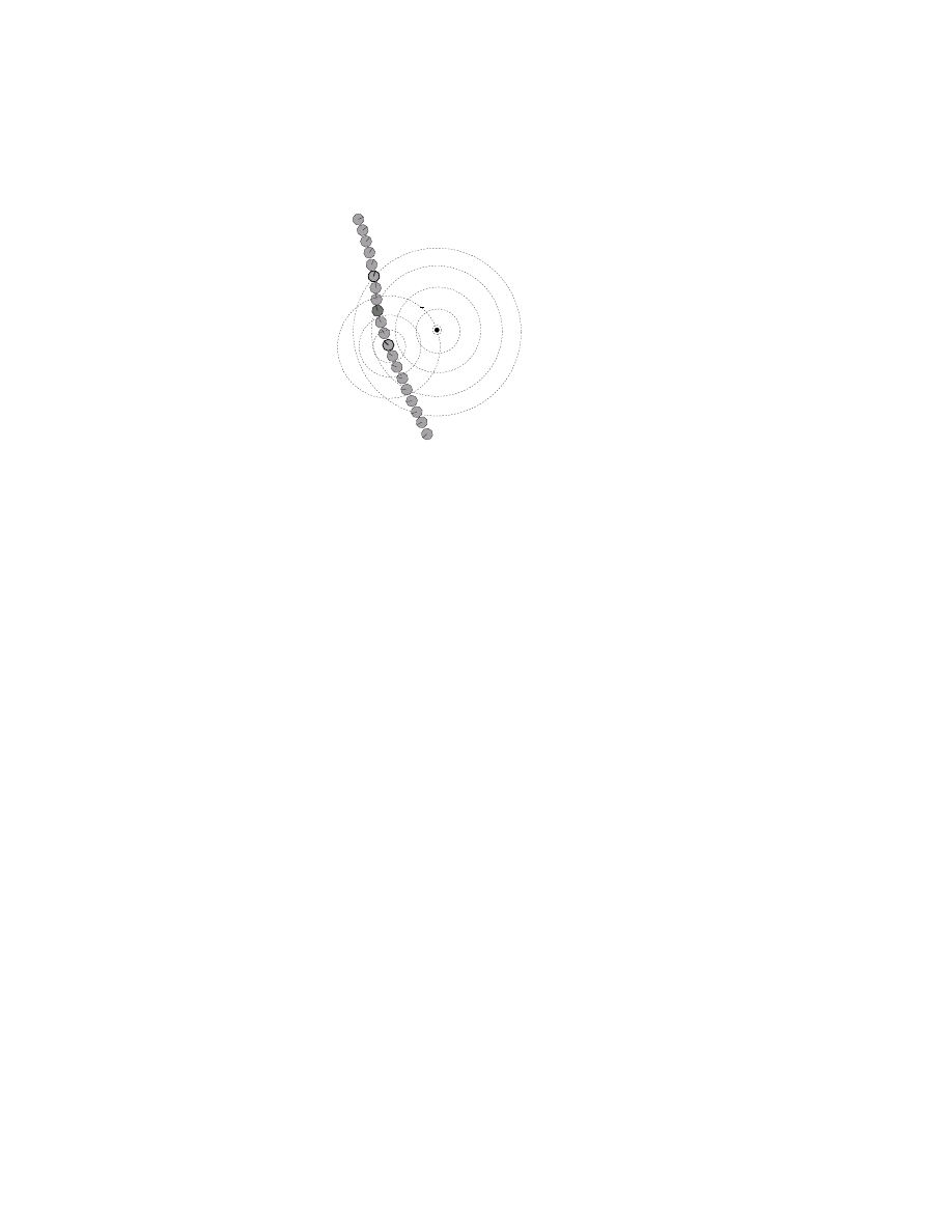
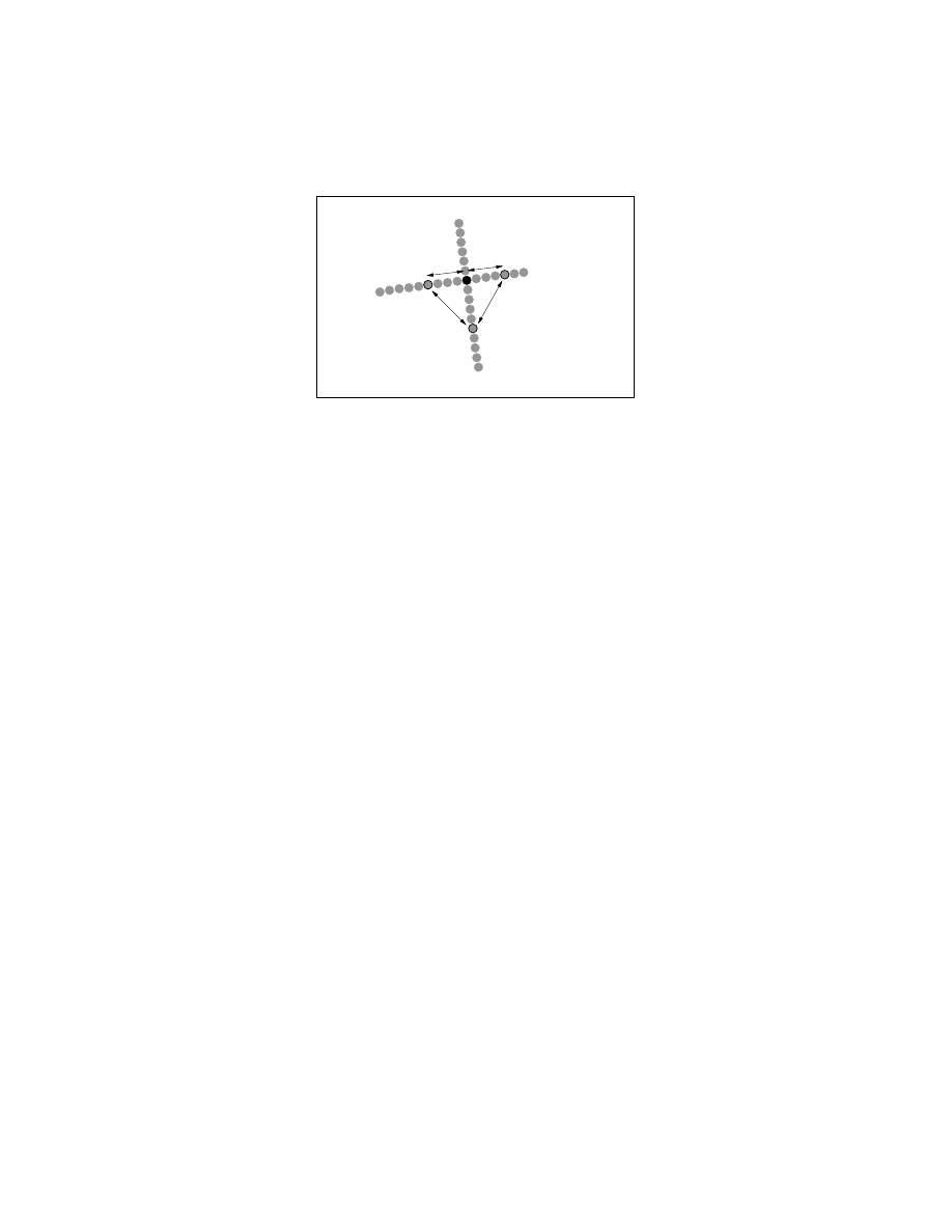
Figure 1: Operational definition of time tags. (This is just a symbolic sketch, not a real
“two dimensional space-time diagram” or the like.)

and distance. (See Brown 2005, pp. 11-14.) We do not dwell on this problem here.
The reader can easily imagine various operational solutions of how to use a marker for
marking various physical events/phenomena.

2.1

Time

Consider the experimental arrangement in Fig. 1. The marker at the standard clock
emits a radio signal at clock-reading t

(event A). The signal is received by another

marker which immediately emits another signal (event B). This “reflected” signal is
detected by the marker at the standard clock at t

(event C). We assume, as an empirical

fact, that the clock we have chosen is such that a given reflected signal is received by
the standard clock only once, at reading t

, and

≥ t

(1)

by which we have chosen, conventionally, an “arrow of time” (not the arrow of physical
processes in time; see Price 1996, p. 16 and 58). (In fact, we made two choices
here. One is the choice of the direction of the parametrization of the clock’s pointer
positions (1). There is however a more important one: by applying the terms “sending”
and “receiving” a signal, we previously determined the causal order of events A and

. To what extent this causal order is purely conventional? How can we—without

prior spatio-temporal conceptions—distinguish whether an event is a “sending” or a
“receiving” of a signal? How is this choice of causal order related to the change of
information content of the signal? To what extent this choice is determined by our free
will and free action experience at the modulation of the radio waves? Is this freedom
an objective openness of future or merely a subjective experience? These are delicate
metaphysical questions into the discussion of which it is not our present purpose to
enter.)

Definition (A1)

The absolute time tag of event B is the following:

τ (B) := t

+ ε (t

−t

)

(2)

where ε =

1
2

by convention. (Of course, it could be a contingent fact of nature that

= t

, in which case the choice of the value of ε would not matter.)

It is important to emphasize that the choice of using radio signals in definition

(A1) is purely conventional. This choice is by no means justified by the “constancy
and isotropy of the (round-trip) velocity of light”; simply because we are prior to any
spatio-temporal concepts that would make any statement about the “velocity” of light
meaningful.

2.2

Distance and the problem of “rest”

Denote S

the set of simultaneous events with time tag τ. One might think that we

are ready to define the spatial distance between two points of space, that is distance
between two simultaneous events. Surely, we can define the distance between the
simultaneous events D and B in Fig. 1 as

1
2

−t

) c, where the value of c is taken

as a convention. In this way however, as a little reflection shows, we can define the
distance only from the standard clock, but there is no way to extend this definition
for arbitrary pair of simultaneous events. In order to define the distance between two
arbitrary simultaneous events we need further preparations.

We would like to base the definition of distance to the definition of time: the dis-

tance between two points in a given S

will be defined through the period of time in

which a radio signal runs “from the one point to the other”. Therefore, instead of sig-
nals sent and received by the marker at the standard clock, we will use radio signals
“sent from the one point and received at the other”. However, we encounter the follow-
ing difficulty. We would like to define distance between simultaneous events; but the
travel of the signal takes some time; the emission of the signal and the receiving of the
signal are not simultaneous events. Whose distance is the one measured by the time of
travel of the signal—and when? The distance obtained by means of the time of travel
of the signal depends on the concept of “rest”; the concept of “being at the same place
at different times” (Fig 2). So, in order to define the distance of simultaneous events
we need a previous concept of “rest”; and, moreover, we have to define this concept by
the only means of the standard clock and radio signals.

It is necessary to be careful of a possible misunderstanding. Although they are

close to each other, the problem we are addressing here is different from the problem
of persistence of physical objects (Butterfield 2005). What we would like to define is
the identity of two locuses of space at two different times, and not the genidentity of
the physical objects occupying these locuses. One might think that some definition of
genidentity of physical objects must be prior to our operational definition of space and
time tags, at least in the case of the standard clock. This is, however, not necessarily the
case. The standard clock is just an ordered (ordered by the clock readings) sequence
of physical events, but without the further metaphysical assumption that these events
belong to the same physical object. (We definitely do not make such assumption in the
case of a “clock-like” sequence of events that we will call a time sequence below.)

standard clock

d(A

, B)

“rest

”

“rest

”

′

′′

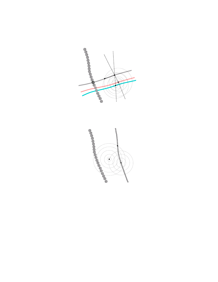
Figure 2: The distance defined by means of the time of travel of the radio signal depends
on the concept of “rest”; the concept of “being at the same place at different times”

In general, τ (B)

− τ (U

)

6= τ (B) − τ (U

)

τ (C)

τ (A)

γ(τ )

standard clock

Figure 3: Clock-like time sequence

Definition (A2)

A one-parameter family of events γ(τ) is called time sequence if

γ (τ )

∈ S

for all τ.

One has to recognize that a time sequence is a “clock-like” sequence of events. For

every event, one can define a time-like tag in the same way as (A1): Event A (Fig. 3)
is marked with the emission of a radio signal at time τ(A). The signal is reflected at
event B. Event C is the first detection of the reflected signal at time τ(C). We define
the following time-like tag for event B:

(B) := τ(A) + ε (τ(C)

− τ(A))

τ (V )

γ(τ )

standard clock

(A,

τ (U )

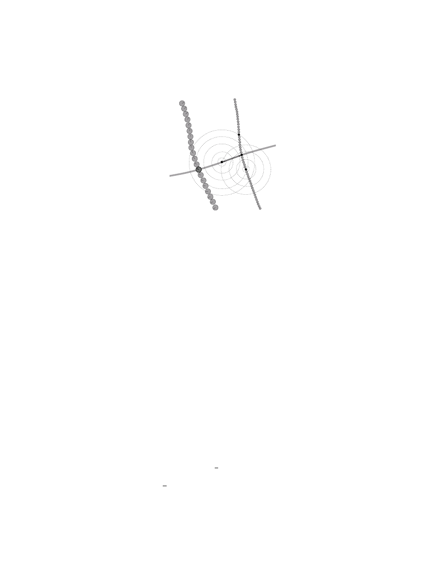
Figure 4: The distance between two simultaneous events

(If there is no detection of the reflected signal at all, then, say, τ

(B) := ∞.)

It is an empirical fact that τ

(B)

6= τ(B) in general. It is another empirical observa-

tion however that for some particular cases τ

(B) = τ(B).

Definition (A3)

A time sequence γ(τ) is a rest time sequence if for every event B

(B) = τ(B).

Whether or not there exist rest time sequences is an empirical question. We stipulate
the following:

Empirical fact (E1)

For any event A there exists a unique rest time sequence γ(τ)

such that A = γ (τ(A)).

Rest time sequence is a concept defined only by means of the standard clock and

radio signals. It singles out a “world line” through every event, that will play the role
of the “world line of a particle being at rest relative to the standard clock”.

Now we are ready to define the distance between simultaneous events.

Definition (A4)

The absolute distance between two simultaneous evens A, B

∈ S

is operationally defined in the following way. Take a rest time sequence γ such that
A

= γ(τ) (Fig. 4). Let U = γ (τ(U)) be an event marked with the emission of a radio

signal at absolute time τ(U ), such that the signal is received and reflected at event B.
The detection of the reflected signal marks the event V = γ (τ(V )) of time tag τ(V ).
The absolute distance is

(A, B) :=

(τ(V )

− τ(U))c

(3)

where c = 299792458

by convention.

We know from (1) that for all A, B

∈ S

(A, B)

≥ 0

(4)

(A, A)

(5)

However, the following facts cannot be known without further empirical observations:

Empirical fact (E2)

For all A, B,C

∈ S

(A, B)

0 only if A = B

(6)

(A, B) + d

(B,C)

≥ d

(A,C)

(7)

(A, B)

(B, A)

(8)

The following proposition is however derivable:

Lemma 1

Let γ

and γ

be arbitrary two rest time sequences. For any two moments

of absolute time τ and τ

(γ

(τ) , γ

(τ))

, γ

(9)

Having distance defined on a given S

, we introduce the following abbreviations:

Cong

(A, B,C, D)

⇐⇒ d

(A, B) = d

(C, D)

Bet

(A, B,C)

⇐⇒ d

(A,C) = d

(A, B) + d

(B,C)

In terms of these abbreviations we formulate the following—not necessarily new—
empirical facts:

(E3)

∀A∀B Cong

(A, B, B, A)

(E4)

∀A∀B∀C Cong

(A, B,C,C)

→ A = B

(E5)

∀A∀B∀C∀D∀E∀F Cong

(A, B,C, D)

∧Cong

(C, D, E, F)

→ Cong

(A, B, E, F)

(E6)

∀A∀B Bet

(A, B, A)

→ A = B

(E7)

∀A∀B∀C∀D∀E Bet

(A, D,C)

∧ Bet

(B, E,C))

→ ∃F (Bet

(D, F, B)

∧ Bet

(E, F, A)

(E8)

∃E∀A∀B A ∈ α ∧ B ∈ β → Bet

(E, A, B)

→ ∃F∀A∀B A ∈ α ∧ B ∈ β → Bet

(A, F, B)

where α and β are two sets of events in S

(E9)

∃A∃B∃C∃D∃E ¬D = E ∧Cong

(A, D, A, E)

∧Cong

(B, D, B, E)

∧Cong

(C, D,C, E)

∧¬Bet

(A, B,C)

∧ ¬Bet

(B,C, A)

∧ ¬Bet

(C, A, B)

(C, B)

(A, C)

(A, B)

Figure 5: Straight line

(E10)

∀A∀B∀C∀D∀E∀F ¬D = E ∧ ¬D = F ∧ ¬E = F
∧Cong

(A, D, A, E)

∧Cong

(A, D, A, F)

∧Cong

(B, D, B, E)

∧Cong

(B, D, B, F)

∧Cong

(C, D,C, E)

∧Cong

(C, D,C, F)

→ Bet

(A, B,C)

∨ Bet

(B,C, A)

∨ Bet

(C, A, B)

(E11)

∀A∀B∀C∀D∀E∀F Bet

(A, B, F)

∧Cong

(A, B, B, F)

∧Bet

(A, D, E)

∧Cong

(A, D, D, E)

∧Bet

(B, D,C)

∧Cong

(B, D, D,C)

→ Cong

(B,C, F, E)

(E12)

∀A∀B∀C∀D∀E∀F∀G∀H ¬A = B ∧ Bet

(A, B,C)

∧Bet

(E, F, G)

∧Cong

(A, B, E, F)

∧Cong

(B,C, F, G)

∧Cong

(A, D, E, H)

∧Cong

(B, D, F, H)

→ Cong

(C, D, G, H)

(E13)

∀A∀B∀C∀D∃E Bet

(D, A, E)

∧Cong

(A, E, B,C)

The quantification runs over S

. In brief, we stipulate, as an empirical fact, that the

two relations Cong

and Bet

, determined by the distances of simultaneous events,

satisfy the axioms of 3-dimensional Euclidean geometry, namely Tarski’s axioms of
3-dimensional Euclidean geometry (Tarski and Givant 1999). It must be emphasized
that all the statements (E3)–(E13) are stipulated, via inductive generalization, merely
on the basis of observations about distances of simultaneous events.

2.3

Spatial coordination

Within this axiomatic framework, one can define the basic geometrical concepts in the
usual way; and one can derive a body of theorems, well known from the textbooks on
Euclidean geometry. Below are a few of the typical definitions and theorems we will
use in the construction of space tags.

Figure 6: Orthogonal lines

Definition

subset σ

⊂ S

is called (straight) line if satisfies the following condi-

tions (Fig. 5):

1. for any A, B,C

∈ σ exactly one of the following three relations hold:

(A,C) + d

(C, B)

(A, B)

(A, B) + d

(B,C)

(A,C)

(B, A) + d

(A,C)

(B,C)

2. σ is maximal for property 1.

Definition

Let σ

and σ

be two lines in S

such that σ

∩ σ

{O} (Fig. 6). σ

orthogonal

to σ

if for every Z

∈ σ

and for every X ,Y

∈ σ

(X , O) = d

(O,Y )

⇔ d

(X , Z) = d

(Y, Z)

Theorem

For every A, B

∈ S

there exists a unique line containing A and B.

Theorem

Let A

∈ S

be an arbitrary event and let σ

⊂ S

be an arbitrary line. There

always exists a line σ

orthogonal to σ

, such that A

∈ σ

Definition

Using the notations of the above theorem, let σ

∩ σ

{O}. Event O is

called the orthogonal projection of A to σ

. Distance d

(A, O) is called the distance of

A from σ

Definition

Let σ

⊂ S

be a line. A line σ

is parallel to σ

if for all X

∈ σ

the

distance of X from σ

is the same.

Theorem

Let σ

⊂ S

be a line and let C

∈ S

be an arbitrary event. There exists

exactly one line σ

such that C

∈ σ

and σ

is parallel to σ

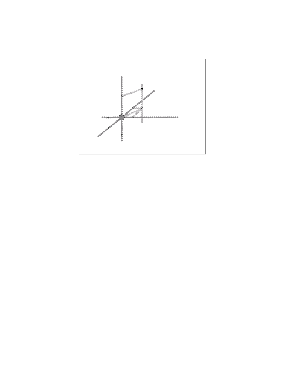
Figure 7: Cartesian coordinates in S

Definition

Let A, B

∈ σ be two events on line σ. Line segment between events

, B

∈ S

is the following subset of σ :

σ (A, B) :=

{ X ∈ σ|d

(A, X ) + d

(X , B) = d

(A, B)

}

(10)

These are however only examples. In what follows, the whole usual system of

definitions and theorems of Euclidean geometry are supposed to be known.

Now we are going to define the standard Cartesian coordinates in S

. First we need

a 3-frame.

Definition (A6)

A 3-frame in S

consists of three pairwise orthogonal lines σ

, σ

in S

, such that σ

∩ σ

{O} and three events X,Y,Z 6= O such that X ∈ σ

∈ σ

and Z

∈ σ

. O is called the origin of the frame (Fig. 7). Let us introduce the

following notations:

{P ∈ σ

|Bet

(X , O, P)

}

−

\ σ

∪ {O}

P ∈ σ

|Bet

(Y, O, P)

−

\ σ

∪ {O}

{P ∈ σ

|Bet

(Z, O, P)

}

−

\ σ

∪ {O}

The origin of the 3-frame is arbitrary, although it is a natural choice to take the “τ-
event” of the standard clock as origin.

In the following definition we give the operational definition of space tags in one

given S

. Let us call them τ-space tags.

Definition (A7)

Let A be an arbitrary event in S

. Take a line segment σ (B,C)

3 A

parallel to σ

(Fig. 7). Take another line segment σ (A, D) orthogonal to σ

such that

∈ σ

. Let σ (O, E) be a line segment parallel to σ (A, D) such that E

∈ σ(B,C).

Finally, take the line segments σ (E, F) and σ (E, G) such that σ (E, F) is parallel to

and F

∈ σ

, and σ (E, G) is parallel to σ

and G

∈ σ

. Now, the τ-space tags are

defined as follows:

(A)

(G, O)

∈ σ

−d

(G, O)

∈ σ

−

(A)

(F, O)

∈ σ

−d

(F, O)

∈ σ

−

(A)

(D, O)

∈ σ

−d

(D, O)

∈ σ

−

It must be emphasized that with the above definitions we only defined the space

tags in a given set of simultaneous events S

. Yet, we have no connection whatsoever

between two S

and S

if τ

6= τ

. In principle, there exist “infinitely” many possible

bijections between the different S

’s. This is true, even if we prescribe that the bijection

must be an isomorphism preserving distances.

Intuitively, a time sequence γ(τ) satisfying that

(γ(τ))

const.

(11)

(γ(τ))

const.

(12)

(γ(τ))

const.

(13)

corresponds to a localized physical object being at rest. “At rest”—relative to what?
The actual behavior described by these equations depends on how the different 3-
frames are chosen in the different S

’s. One might think that an object is at rest if

equations (11)–(13) hold in one and the same 3-frame in all S

. But, what does it mean

that “one and the same 3-frame in all S

”? When can we say that a line segment σ

is the same 3-frame axis as σ

in S

? When can we say that an event A

is in the

same place in S

as event A in S

When we are seeking for a correspondence between S

and S

, our aim is not

simply to find a mathematically “canonical” bijection—whatever it means. What we
wish is a one-to-one map

: S

→ S

of natural physical meaning:

(a)

It must be defined by means of physical operations.

(b)

For all A, B

∈ S

, we require that d

(A) , T

(B)

= d

(A, B).

(c)

It must reflect our intuition about being “at rest”. (For example, in our tradi-
tional language, if the standard clock moves along a time-like straight line of the
Minkowski space-time, T

must be equal to the map (τ, x, y, z)

7→ (τ

, x, y, z), in

the frame of reference of the standard clock. Of course, this example should be
understood only intuitively.)

We have already defined a concept of the unique rest time sequence through every
event. So, condition (c) basically means that for any rest time sequence γ we require
that T

(γ(τ)) = γ (τ

). In fact, we will base the connection between different time

slices on the rest time sequences:

Definition (A8)

: S

→ S

7→ T

(A) = γ(τ

)

where γ is a rest time sequence such that A = γ(τ). Let us call T

the time shift between

and S

. It follows from (E1) and Lemma 1 that this definition is sound and T

is a

distance preserving bijection. Now we have everything at hand to define the space tags
of events:

Definition (A9)

Let A be an arbitrary event. The absolute space tags of A are defined

as follows:

(A)

0
τ (A)

(A)

0
τ (A)

(A)

0
τ (A)

(A)

Thus, we are given the absolute space and time tags for every event: ξ

(A), ξ

(A),

(A), τ(A).

Inertial motion

A remark is in order on the empirical facts (E1)–(E13) to which we refer in construct-
ing the space and time tags. When I call them empirical facts I mean that they ought to
be true according to our ordinary physical theories. The ordinary physical theories are
however based on the ordinary, problematic, space and time conceptions, relaying on
“reference frames realized by rigid bodies” and the likes, without proper, non-circular,
empirical definitions. Thus, especially in the context of defining the two most funda-
mental physical quantities, distance and time, we must not regard our ordinary physical

theories as empirically meaningful and empirically confirmed claims about the world.
Whether these statements are true or not is, therefore, an empirical question, and it is
far from obvious whether they would be completely confirmed if the corresponding
experiments were performed with higher precision, similar to the recent GPS measure-
ments, especially for larger distances. Strangely enough, according to my knowledge,
these very fundamental facts have never been tested experimentally; no textbook or
monograph on space-time physics refers to such experimental results.

So, the best we can do is to believe that our physical theories based on the usual

sloppy formulation of spatio-temporal concepts are true (in some sense) and to consider
the predictions of these theories as empirical facts. However, as the following analysis
reveals, it is far from obvious whether the predictions of the believed theories really
imply (E1)–(E13).

Throughout the definition of space and time tags, we avoided the term “inertial”,

and because of a good reason. First of all, if “inertial” is regarded as a kinematical
notion based on the concept of straight line and constancy of velocity, then it cannot be
antecedent to the concept of space-time tags. If, on the other hand, it is understood as a
manner of existence of a physical object in the universe, when the object is undergoing
a free floating, in other words, when it is “free from forces”, then the concept is even
more problematic. The reason is that “force” is a concept defined through the deviation
from the trajectory of inertial motion (first circularity), and neither the inertial trajec-
tory nor the measure of deviation from it can be expressed without spatio-temporal
concepts; consequently, they cannot be antecedent to the definition of space and time
tags (second circularity). So there is no precise, non-circular definition of inertial mo-
tion. It is to be emphasized that this operational/logical circularity is a problem even
in a special relativistic/flat/local space-time; and, therefore, it has nothing to do with
the problem of conventionality of demarcation between “inertial” or “geodetic” motion
versus gravitation as universal force (cf. Märzke and Wheeler’s 1964).

According to our believed special relativistic physical theory, space-time is a 4-

dimensional Minkowski space and inertial trajectory is a time-like straight line in the
Minkowski space. Since we are prior to the empirical definitions of the basic spatio-
temporal quantities, we cannot regard this claim as an empirically confirmed physical
theory. Nevertheless, let us assume for a moment that our special relativistic theory
is the true description of the world “from God’s point of view”. It is straightforward
to check that all the facts (E1)–(E13) are true if 1) the standard clock moves along an
inertial world line in the Minkowski space-time and 2) it reads the proper time, that
is, it measures the length of its own word line, according to the Minkowski metric.
However, we human beings can know neither whether the standard clock (chosen by
us) is of inertial motion in God’s Minkowskian space-time nor whether it reads the
proper time. What if these conditions fail? What does special relativistic kinematics
say about (E1)–(E13) if the standard clock is accelerated and/or it does not read the
proper time?

In order to answer this question, we have to follow up the operational definitions

(A1), (A2),. . . and calculate whether statements (E1), (E2),. . . are true or not if the
standard clock moves along a given world line γ and the “time” it reads is, say, a given
function of the Minkowskian coordinate time, χ(t). Although the task is straightfor-

ward, the calculation is too complex to give a general answer in details. Fortunately,
we do not need all the details: the essential fact is that if we really can go through the
whole operational procedure, and (E1)–(E13) are true, then, at the end, we obtain a
coordination of events such that the equation describing the trajectory of a signal in the
space of the four coordinates is

(ξ

(τ)

− ξ

)

+ (ξ

(τ)

− ξ

)

+ (ξ

(τ)

− ξ

)

= c

Now, due to the Alexandrov–Zeeman theorem (Alexandrov 1950; Zeeman 1964), one
can derive the following results.

Theorem

Facts (E1)–(E13) are true if and only if the standard clock moves along an

inertial world line and reads a time χ(t) which is a linear function of the Minkowskian
coordinate time.

Due to this theorem, in accord with our intuition based on the believed physical the-
ories, we can give an objective meaning to “inertial motion” by means of correct—
neither logically nor operationally circular—experiments: the standard clock is of iner-
tial motion if statements (E1)–(E13) are true.

Assuming that the standard clock is iner-

tial, one can extend the concept for an arbitrary time sequence γ(τ) of events: γ(τ) cor-
responds to an inertial motion if the absolute space tags ξ

(γ (τ)) , ξ

(γ (τ))

are linear functions of the absolute time tag τ.

There is a trivial but very important corollary of the above theorem: Imagine that we

successfully perform two different coordinations of events by means of two different
standard clocks. The theorem implies that the two coordinations are identical up to an
almost Lorentz transformation.

Of course, the Alexandrov–Zeeman theorem applies if all of (E1)–(E13) are satis-

fied. It is perhaps interesting, that the essential condition is (E1). From an analysis by
computer one finds the following result:

Result 1

There are no unique rest time sequences if the standard clock moves non-

inertially in a Minkowski space.

Still, one must emphasize, whether (E1)–(E13) are true or false is an open empir-

ical

question. Imagine that the standard clock is not inertial; for example (E1) is not

satisfied. It would also mean that the clock chosen by us would be inappropriate for the
definition of space-time tags. More exactly, we should have to stop at definition (A1).
We could define the time tags but could not define the spatial notions, in particular the
distances between simultaneous evens. Consequently, it is meaningless to talk about
“non-inertial reference frame”, “space-time coordinates (tags) defined/measured by an
accelerated observer”, and the likes. In the light of these consequences, it is an intrigu-
ing question whether the standard clock contemporary physical laboratories use for the
coordination of physical events satisfies conditions (E1)–(E13), in particular (E1).

Absolute, relative, conventional

I call τ(A) “absolute time” not in the sense of what Newton called “absolute, true and
mathematical time”, that is independent of any empirical definition, but in the sense
of what the 20th century physics calls absolute time; it is “independent of the position
and the condition of motion of the system of co-ordinates” (Einstein 1920, p. 51). The
space and time tags ξ

(A), ξ

(A), τ(A) are absolute in the sense that they are

not relative to a reference frame

but prior to any reference frame. (The concept of

“reference frame” is still not defined, and actually we do not need it.)

Absolute space and time tags are, of course, “relative” to the trivial semantical

convention

by which we define the meaning of the terms. They are “relative” to the

etalon

clock-like process we have chosen in the universe; and to the particular way in

which the space and time tags are defined, including the usage of radio signals, the
choice of “ε =

1
2

”, etc. This kind of “relativism” is however common to all physical

quantities having empirical meaning.

But there are two things that do not follow from this kind of conventionality. On

the one hand, it does not follow that these physical quantities cannot describe objective
features of physical reality; in spite of the obvious fact that these conventions play a
constitutive role in the conceptual representation of the world. On the other hand, it
does not follow either that there are no objective constraints on the semantical conven-
tions themselves. In this last passage, I would like to give an example of how these
objective constraints can restrict the semantical conventions defining absolute space
and time tags.

There has been a long discussion in the literature about the conventionality of si-

multaneity. As it is obvious from (2), we chose the standard “ε =

1
2

-synchronization”.

This choice was a part of the trivial semantical convention defining the term “abso-
lute time tag”. It is, therefore, prior to any claim about the one-way or even round-trip
speed of electromagnetic signals, because there is no such a concept as “speed” prior to
the definition of time and space tags; it is, of course, prior to “the metric of Minkowski
space-time”, in particular to the “light-cone structure of the Minkowski space-time”,
because we have no words to tell this structure prior to the space and time tags; and
it is prior to the causal order of physical events, because—even if we could know this
causal order prior to temporality—we cannot know in advance how causal order is
related with temporal order (which we have defined here). It is actually prior to any
discourse about two locuses in space, because there is no “space” (S

) prior to defini-

tion (A1) and there is no concept of a “persistent space locus” prior to definitions (A3)
and (A8).

So far, it seems, we are entirely free in the choice of the value of ε, that is in

the choice of which objective feature of the physical reality—time

—we want to deal

with. One might think that starting with some ε, that is with some time

tags τ

(A)

and the corresponding ε-simultaneity slices S

ε
τ

, one finally obtains some space

References

Alexandrov, A. D. 1950. On Lorentz transformations. Uspekhi Math. Nauk 5: 187. (in
Russian)
Brown, H. R. 2005. Physical Relativity. Space-time structure from a dynamical per-
spective
. Oxford: Clarendon Press.
Butterfield, J. 2005. On the Persistence of Particles. Foundations of Physics 35: 233.
Einstein, A. 1920. Relativity: The Special and General Theory. New York: H. Holt
and Company. Märzke, R. F. and Wheeler, J. A. 1964. Gravitation as geometry I:
the geometry of spacetime and the geometrodynamical standard meter, in Gravitation
and relativity
, H. Y. Chiu and W. F. Hoffmann (eds.), New York–Amsterdam: W. A.
Benjamin Company.
Price, H. 1996. Time’s arrow and Archimedes’ point: new directions for the physics of
time
. New York, Oxford: Oxford Universoty Press.
Tarski, A. and S. Givant. 1999. Tarski’s system of geometry. Bulletin of Symbolic
Logic
5: 175.
Zeeman, E. C. 1964. Causality implies the Lorentz group. Journal of Mathematical
Physics
5: 490.
16
Wyszukiwarka
Podobne podstrony:
Rucker Master of Space and Time
Rudy Rucker Master Of Space And Time
To Love Through Space and Time Tinnean
Quest Through Space and Time Clark Darlton
Chordia, Sarkar And Subrahmanyam An Empirical Analysis Of Stock And Bond Market Liquidity
How to Save Money Hundreds of Money and Time Saving Hints
Hawking S Space and time warps (public lecture)(6s)
Isaac Asimov Of Time and Space and Other Things
Asimov, Isaac Of Time and Space and Other Things(1)
Asimov, Isaac Of Time and Space and Other Things
UTC?te and time of solstices and equinoxes
Modeling and minimizing process time of combined convective and vacuum drying of mushrooms and parsl
Method of gravity distortion and time displacement United States Application US20060073976
Eurocode 8 Part 5 1998 2004 Design of Structures for Earthquake Resistance Foundations, Retaini
Wójcik, Marcin Rural space and the concept of modernisation Case of Poland (2014)
Dennett s response to Bennett and Hacker s Philosophical Foundations of Neuroscience
więcej podobnych podstron