The Stirling Engine-Refrigerator: Rich Pedagogy from Applied Physics

http://xxx.lanl.gov/html/physics/0112061

1 sur 20

29/11/2006 11:09

arXiv:

physics/0112061

v1 19 Dec 2001

The Stirling Engine-Refrigerator: Rich Pedagogy from Applied Physics

Randall D. Peters

Department of Physics

1400 Coleman Ave.

Mercer University

Macon, Georgia 31207

Abstract

A Stirling engine of the type used for demonstration purposes has been outfitted with a pair of sensors that measure pressure and piston displacement when the
engine is operating with a small temperature difference between the hot and cold reservoirs. Measured variables are compared against computer generated
output based on a simple theory that involves nonlinear equations of motion. Theory and experiment are found to be in reasonable agreement. Temperature
dependence of the graph of pressure versus piston displacement, for different directions of flywheel rotation, permits a better understanding of the physics of
heat engines and refrigerators in general.

1 Introduction

One of the most elegant Stirling engines is a style which works with a low temperature difference,

∆

T, between the hot and cold reservoirs. Such an engine,

used for demonstration purposes, is quite impressive when seen to run with only the heat supplied by one's hand. Such engines can be easily instrumented with
sensors to allow comparison between theory and experiment. For example, the present paper describes an engine in which simultaneous measurements were
made of chamber pressure and piston displacement using capacitance sensors. The output from the sensors were fed to a computer through an interface, so
that each of these variables was either graphed as a function of time or plotted one versus the other. The latter case of pressure versus piston displacement is
well suited to comparing theory with experiment, and is closely related to the graphs commonly encountered in the study of thermodynamics. Additionally,
however, by centering the hysteresis curve on the origin, such plots are closely allied with real springs that possess hysteresis, as opposed to Hooke's law
(idealized) systems. For

∆

T = 0, the hysteresis curve is traversed counterclockwise because of friction, and the area inside the loop is proportional to the

work done against friction per cycle. In this case there is no asymmetry associated with direction of flywheel rotation. For

∆

T

>

0, the symmetry is broken

and the direction of hysteresis traversal is clockwise for flywheel rotation corresponding to a heat engine. In this case the friction is overcome by heat transfer.
On the other hand, for flywheel rotation in the opposite direction, an external torque is necessary to sustain the motion, and the magnitude of

∆

T can be

The Stirling Engine-Refrigerator: Rich Pedagogy from Applied Physics

http://xxx.lanl.gov/html/physics/0112061

2 sur 20

29/11/2006 11:09

increased if the work done by the external torque is sufficiently large; i.e., the system is then functioning as a refrigerator or heatpump.

2 The Engine

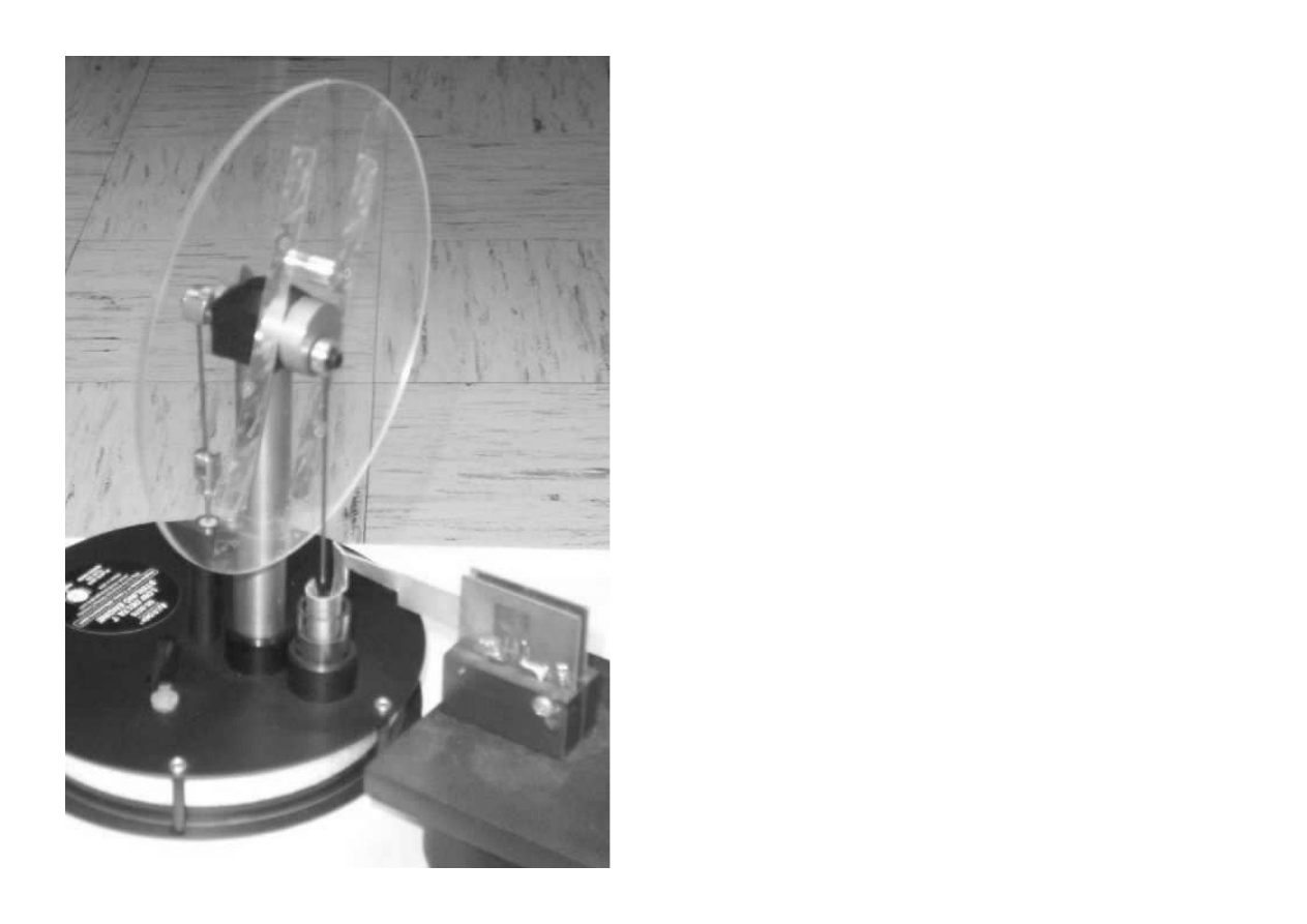
A picture of the engine used for the experiment is provided in Figure 1. It is the Low Delta T Model MM-6 of the American Stirling Company. Shown to its
right is the capacitive sensor that was used to measure piston position. Not pictured is a different sensor which was used to measure engine pressure by
connecting it, via tygon tubing, to the small plastic port which was added to the engine by drilling and tapping a small hole in the top face (seen in the
foreground).

The Stirling Engine-Refrigerator: Rich Pedagogy from Applied Physics

http://xxx.lanl.gov/html/physics/0112061

3 sur 20

29/11/2006 11:09

The Stirling Engine-Refrigerator: Rich Pedagogy from Applied Physics

http://xxx.lanl.gov/html/physics/0112061

4 sur 20

29/11/2006 11:09

Figure 1. Photograph of the engine.

For the picture, the housing of the position sensor was displaced right and forward, permitting a partial view of the rectangular electrode that is attached to the
piston, and which moves vertically between the static plates of the sensor. This moving electrode was fabricated from thin sheet aluminum, and a conical
appendage was formed for it to press-fit into the hollowed-out top of the graphite piston.

Evident in the Figure 1 photograph are some notable characteristics, such as the two connecting rods attached at their tops to a pair of crankshafts on opposite
faces of the flywheel. One rod goes to the piston, whose position is measured; and the other rod goes to the large diameter `foam displacer', whose white edge
is easily seen inside the cylinder of the engine. The displacer fits very loosely inside the cylinder, which is formed by clamping the top and bottom
black-anodized metal plates on opposite sides of a thin-wall acrylic member. By contrast, the piston fits snugly, but with low friction, inside its small glass
cylinder. As the flywheel rotates, each of the piston and the displacer executes cyclic motion, and there is a 90 degree phase difference between them. When
moving, the porous displacer shuttles air back and forth between the hot and cold plates. For most of the present experimental cases, the bottom plate sat on
an electric hot-plate, which was used to raise its temperature. The top plate for these cases was maintained nearly at room temperature.

The cyclic motion of the piston is of constant amplitude, and the period depends on the speed of flywheel rotation. The pressure variation is also cyclic with a
period determined by the angular speed of the flywheel, but the amplitude of the pressure variations increases with an increase of the temperature difference.

3 Theoretical Model

The Stirling Engine-Refrigerator: Rich Pedagogy from Applied Physics

http://xxx.lanl.gov/html/physics/0112061

5 sur 20

29/11/2006 11:09

h

2

= R

2

+Y

2

- 2YR cos

θ

which for R

<<

Y

min

= h yields

y = h - Y

≈

- R cos

θ

τ

= RF sin

θ

= I

..

θ

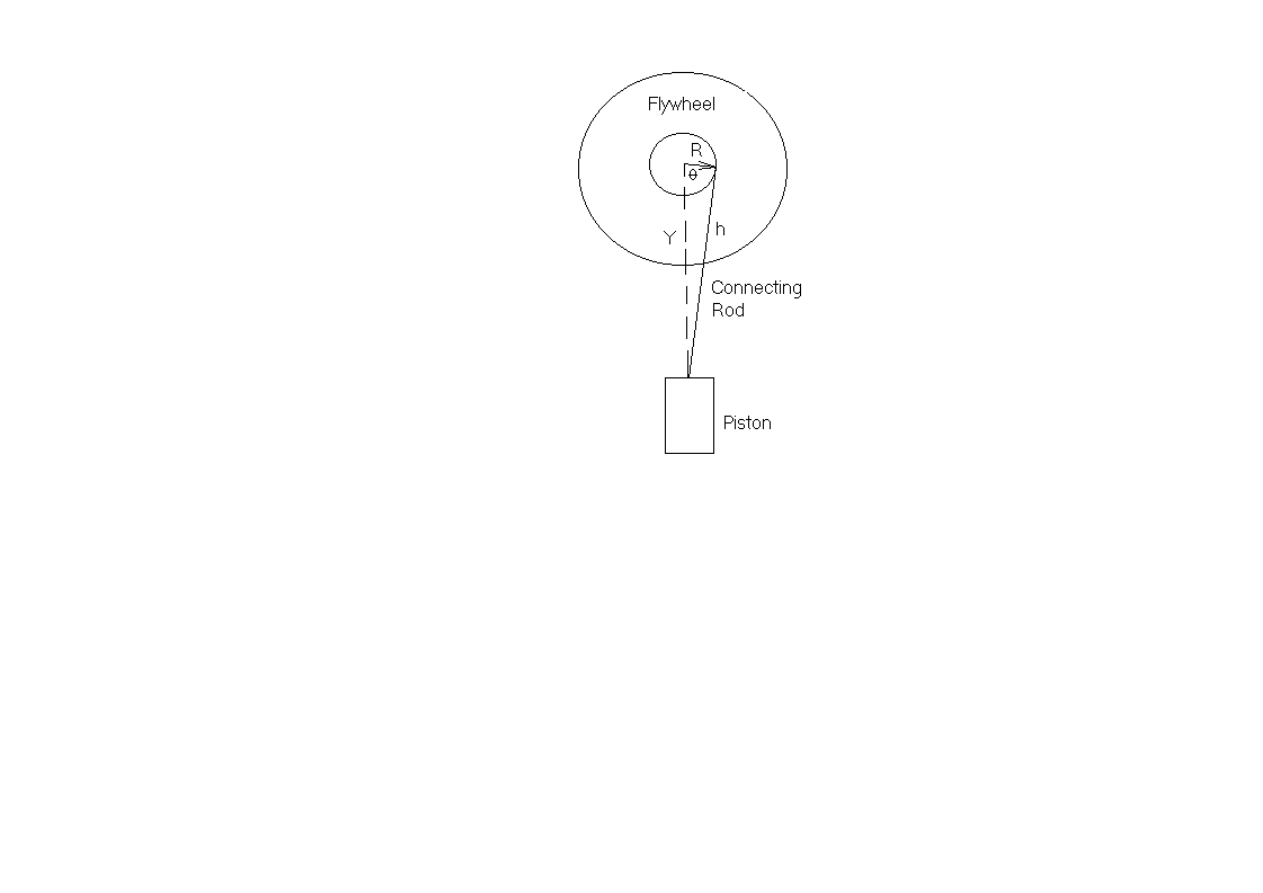
The linkage between piston and crankshaft is illustrated in Figure 2.
Figure 2: Crankshaft and Piston Geometry

The stroke is determined by the offset R of the top of the connecting rod. Using the law of cosines, one obtains the position y of the piston:

(1)

For the small R approximation indicated in Eq.(1), the torque acting on the flywheel due to the piston force F is given by

(2)

where Newton's second law (rotation) has been applied, assuming the only significant mass is that of the flywheel, which has a moment of inertia, I.

The Stirling Engine-Refrigerator: Rich Pedagogy from Applied Physics

http://xxx.lanl.gov/html/physics/0112061

6 sur 20

29/11/2006 11:09

V =

1

4

π

D

2

t (f +

d

2

tD

2

y) = V

0

(f +

ρ

y)

δ

P = -

NkT

0

V

0

f

2

ρ

y +

Nk

V

0

f

δ

T = -

P

0

ρ

y

f

+

P

0

T

0

δ

T

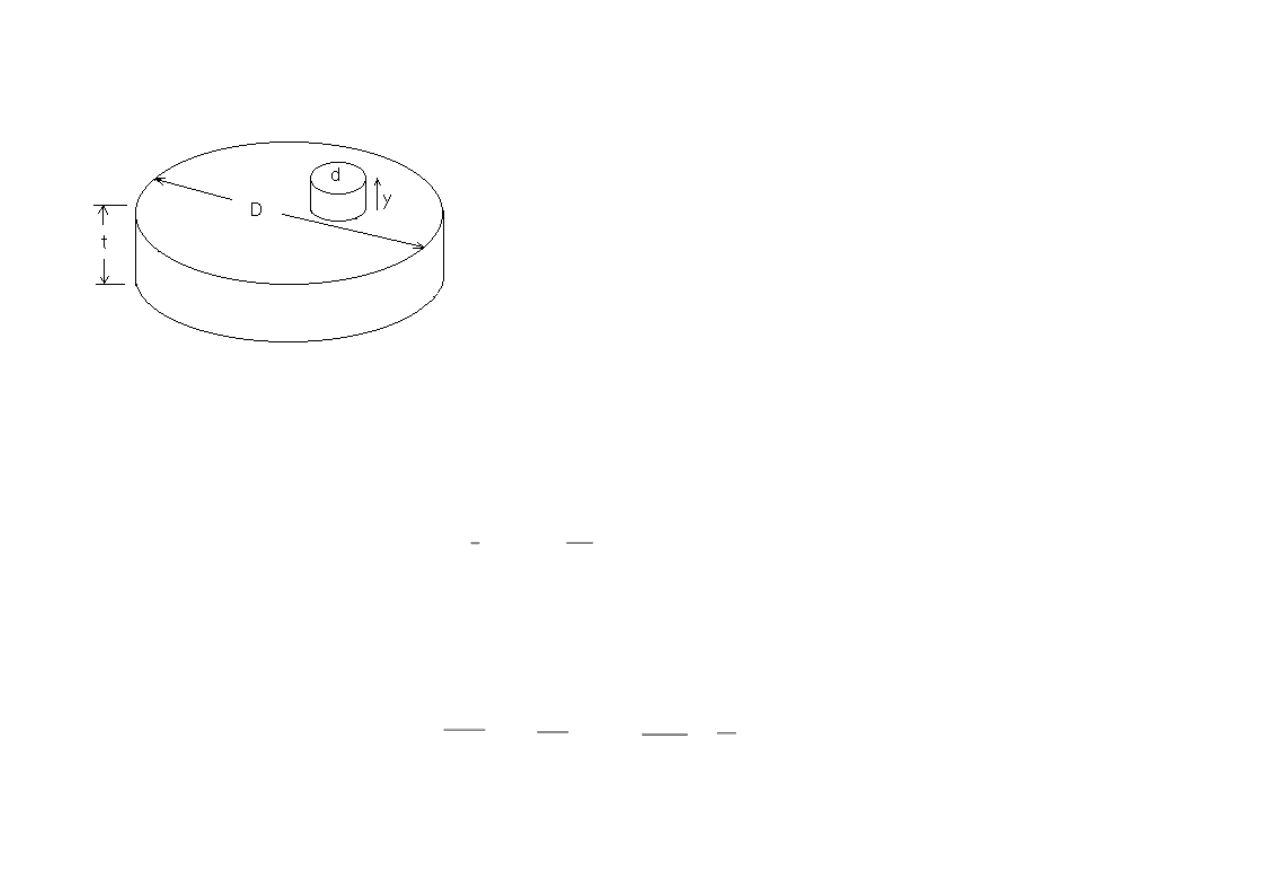
To estimate F, we consider the housing geometry, shown in Figure 3.

Figure 3: Housing geometry

The diameter of the cylinder housing the displacer has been labeled D and its thickness t, and the diameter of the piston d. Estimates of the volume of the
working gas are complicated by the porosity of the displacer. We assume that it is given by

(3)

where the fraction, f

<

1, was determined by trial and error through comparison of theory and experiment.

The force F applied to the crankshaft by the piston is calculated by applying the ideal gas law P V = N k T to the air in the cylinder, to obtain the pressure
change in terms of piston displacement and temperature difference as

(4)

where P

0

= 1.01×10

5

Pa, T

0

= 300 K,

δ

V/V

0

=

ρ

y, and it has been assumed that

ρ

y

<<

1.

The Stirling Engine-Refrigerator: Rich Pedagogy from Applied Physics

http://xxx.lanl.gov/html/physics/0112061

7 sur 20

29/11/2006 11:09

F = -

π

Nkd

2

4V

0

f

(

T

0

ρ

y

f

-

δ

T)

δ

T =

∆

T

.

y

2

|

.

y

max

|

=

∆

T

.

y

2 R

ω

.

ω

=

C R

2

T

0

ρ

I f

sin 2

θ

+

∆

T

C R

I

sin

2

θ

,

.

θ

=

ω

, C =

π

Nkd

2

8V

0

f

=

π

P

0

d

2

8T

0

y = - R cos

θ

,

.

y

=

ω

R sin

θ

From Eq.(4) the force is then calculated to be

(5)

The instantaneous temperature variation,

δ

T in Eq.(5) is the source of drive for the engine, as it varies between positive and negative values in response to the

motion of the displacer. Because the displacer motion differs in phase from piston motion by

π

/2,

δ

T is expressed in the following form,

(6)

where

∆

T = T

H

-T

L

, is the difference in the `high' temperature of the bottom plate and the `low' temperature of the top plate as currently used. According to

the algebraic sign of

∆

T and the direction of the angular velocity

ω

of the flywheel, the system can function either as a heat engine or as a refrigerator. To

operate as a refrigerator, work must be done through an applied external torque.

To obtain the equations of motion, we combine Eqs.(5 and 6) with Eq.(2) to yield

(7)

which, when integrated, give the piston displacement and velocity according to

(8)

Additionally, we use Eq.(4) with

δ

T calculated using Eq.(6), since the most useful graph for comparing theory and experiment is

δ

P vs y.

The Stirling Engine-Refrigerator: Rich Pedagogy from Applied Physics

http://xxx.lanl.gov/html/physics/0112061

8 sur 20

29/11/2006 11:09

.

ω

=

C R

2

T

ρ

I f

sin 2

θ

+ (

∆

T -

∆

T

0

)

C R

I

sin

2

θ

- C

d0

(

|∆

T

|

+ 1)

x

ω

,

Nonlinearity is present in Eq.(7) through both of the terms sin2

θ

and sin

2

θ

. It is thus expected that an analytic solution would not be trivial, if at all possible.

Consequently, the equations are solved by numerical integration.

3.1 Friction Model

As it stands, Eq.(7) is incomplete, since there has been no account for friction, and

ω

will grow without bound for

δ

T

≠

0. To correct this deficiency, viscous

damping was added to the expression for the angular acceleration; to provide an exponential limit to the average angular speed. It was found that a
temperature dependent coefficient of linear damping was necessary for decent agreement with experiment. Such temperature dependence is expected because
the air of the cylinder experiences ever greater convection as the temperature of the lower plate is increased. In turn, the displacer requires greater
nonconservative forcing against buoyancy to sustain its cyclic motion. The dependence on temperature of this increased damping is undoubtedly complex; but

in this first treatment of the problem, a power law was assumed: C

d

= C

d0

(

|∆

T

|

+ 1)

x

with C

d0

= 0.06 and x = 0.6. Both C

d0

and x were determined

empirically, and their uncertainties are in the neighborhood of 10%.

Additionally, it was necessary to account for the system's departure from Hooke's law when

∆

T = 0. To correct for this, a constant term

∆

T

0

was subtacted

from

∆

T . An inspection of Equations (5 and 6) reveals that this provides for an equivalent viscous damping force. Although this was computationally

convenient, free decay data was found to be more nearly linear than logarithmic, like Coulomb friction. Some of this must derive from (i) the push-rod guides
and (ii) the several bearings and bushings of the engine.

The drive-disabled free-decays were obtained by disconnecting the graphite piston push-rod where it joins the flywheel, and observing the pressure after the
flywheel was given an initial angular velocity by hand spinning. As the temperature was increased, the decay constant was found to also increase; which is
consistent with the temperature dependent friction model.

Thus the d

ω

/d t term in Eq.(7) was modified to the following form:

(9)

It should be noted that the signs on

∆

T and

∆

T

0

must be correctly assigned for the various possibilities of heat engine and refrigerator according to whichever

plate is hotter, top or bottom.

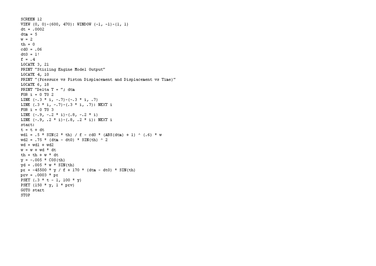
3.2 Software code

Shown in Table I is the QuickBasic software which was used to code the theory. The numerical integration occurs in the loop defined by `start:', and involves
the last point approximation (Cromer modified Euler method) [1]

The Stirling Engine-Refrigerator: Rich Pedagogy from Applied Physics

http://xxx.lanl.gov/html/physics/0112061

9 sur 20

29/11/2006 11:09

TABLE I. Software corresponding to the theory given.

4 Hardware

4.1 Engine parameters

The Stirling Engine-Refrigerator: Rich Pedagogy from Applied Physics

http://xxx.lanl.gov/html/physics/0112061

10 sur 20

29/11/2006 11:09

The various constants for the engine were measured as d = 1.5 cm, D = 14.5 cm, t = 2.4 cm, and y

max

= R = 0.6 cm, from which

ρ

≈

0.45 m

-1

, and V

0

≈

4 ×10

-4

m

3

. The flywheel moment of inertia was estimated to be I

≈

2×10

-4

kg m

2

; and a comparison of theory and experiment

yielded f

≈

0.4, and thus N

≈

4×10

21

. The engine is operated close to room temperature of 295 K. Although the upper plate temperature rises somewhat

above room temperature as the bottom plate is heated; for the present model, the top plate temperature was held constant at T

0

= 300 K.

The compression ratio, V

max

/V

min

≈

1.01, is exceedingly small compared to practical `work-horse' engines.

4.2 Electronics

Both of the sensors used in this experiment were of the symmetric differential capacitive (SDC) type. The piston position was measured with an SDC sensor
that operates on the basis of electrode area variation [2]. The SDC pressure sensor operates on the basis of gap spacing variation [3]. The interface between
these two sensors and the computer was a KIS interface that is sold jointly by TEL-Atomic Inc and Central Scientific.

5 Comparison of Theory and Experiment

5.1 Parameter adjustment

5.1.1 Damping coefficients

Several parameters could be determined only after the engine had been instrumented for data collection. These include the two damping coefficients and the
volume fraction parameter, f. One of the easier parameters to estimate is the coefficient, C

d0

, as follows. With

∆

T = 0 the flywheel was initially spun at about

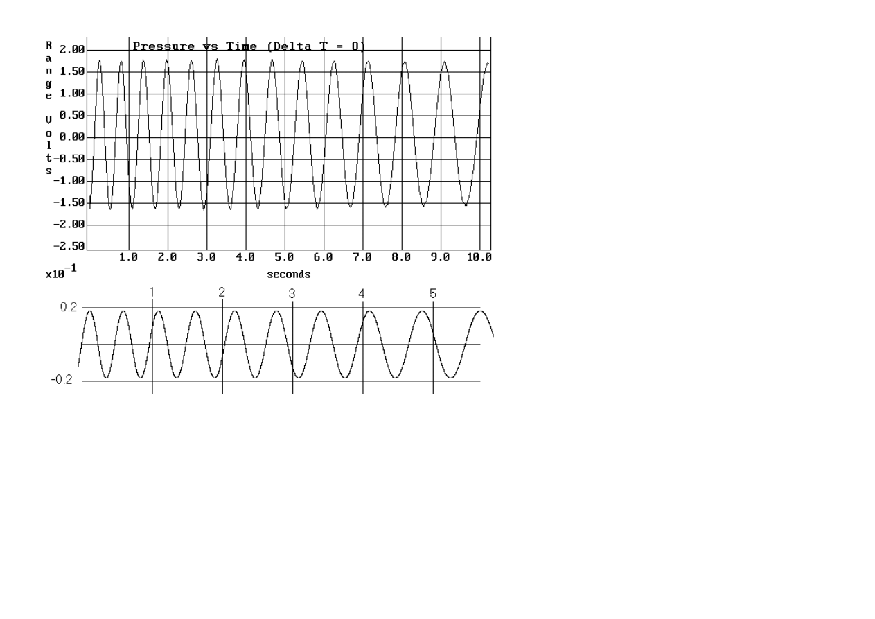
two cycles per second and its deceleration observed in time. The results are shown in Figure 4, where the upper plot is from experiment and the lower one
from theory. For the lower graph the damping coefficient was set at C

d0

= 0.06.

The Stirling Engine-Refrigerator: Rich Pedagogy from Applied Physics

http://xxx.lanl.gov/html/physics/0112061

11 sur 20

29/11/2006 11:09

Figure 4. Comparison of experiment and theory for

∆

T = 0. Both graphs are the time dependence of pressure.

To determine x = 0.6, the exponent for the temperature dependent contribution to the damping in Eq.(9), the steady state value of

ω

was measured at several

temperatures, and then the parameter adjusted in the model for reasonable agreement. For example, for

∆

T = 5 K, the period of flywheel motion at steady

state was measured at approximately 0.75 s, and for

∆

T = 10 K, it was 0.5 s.

The value for the volume fraction, f = 0.4, was obtained by trial and error by comparing model output to measured peak-to-peak pressure variations as a
function of

∆

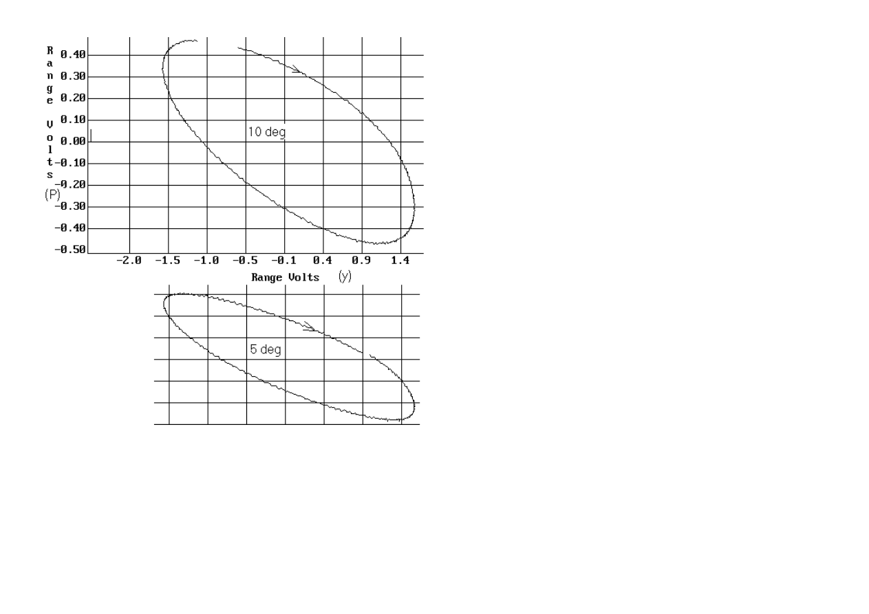
T. The graph most useful for this purpose is the hysteresis curve of pressure vs piston displacement, for which examples are shown in Fig. 5.

The Stirling Engine-Refrigerator: Rich Pedagogy from Applied Physics

http://xxx.lanl.gov/html/physics/0112061

12 sur 20

29/11/2006 11:09

Figure 5. Measured Hysteresis of pressure vs Piston displacement.

The upper curve is for

∆

T = 10 K. The same-scale lower case for

∆

T = 5 K was `pasted' for comparison. The ordinate axis labeled (P) is pressure in volts

output from the sensor. The calibration constant for the pressure sensor was 0.0003 V/Pa, determined by the whirling catheter technique described in the
appendix. Thus the peak-to-peak pressure variation for the 5 K case is 1900 Pa, and for the 10 K case is 3100 Pa.

The abscissa axis (y) is piston displacement in volts output from the SDC position sensor. Since the turning points are at plus and minus 0.6 cm, its calibration
constant is seen to be 2.7 V/cm.

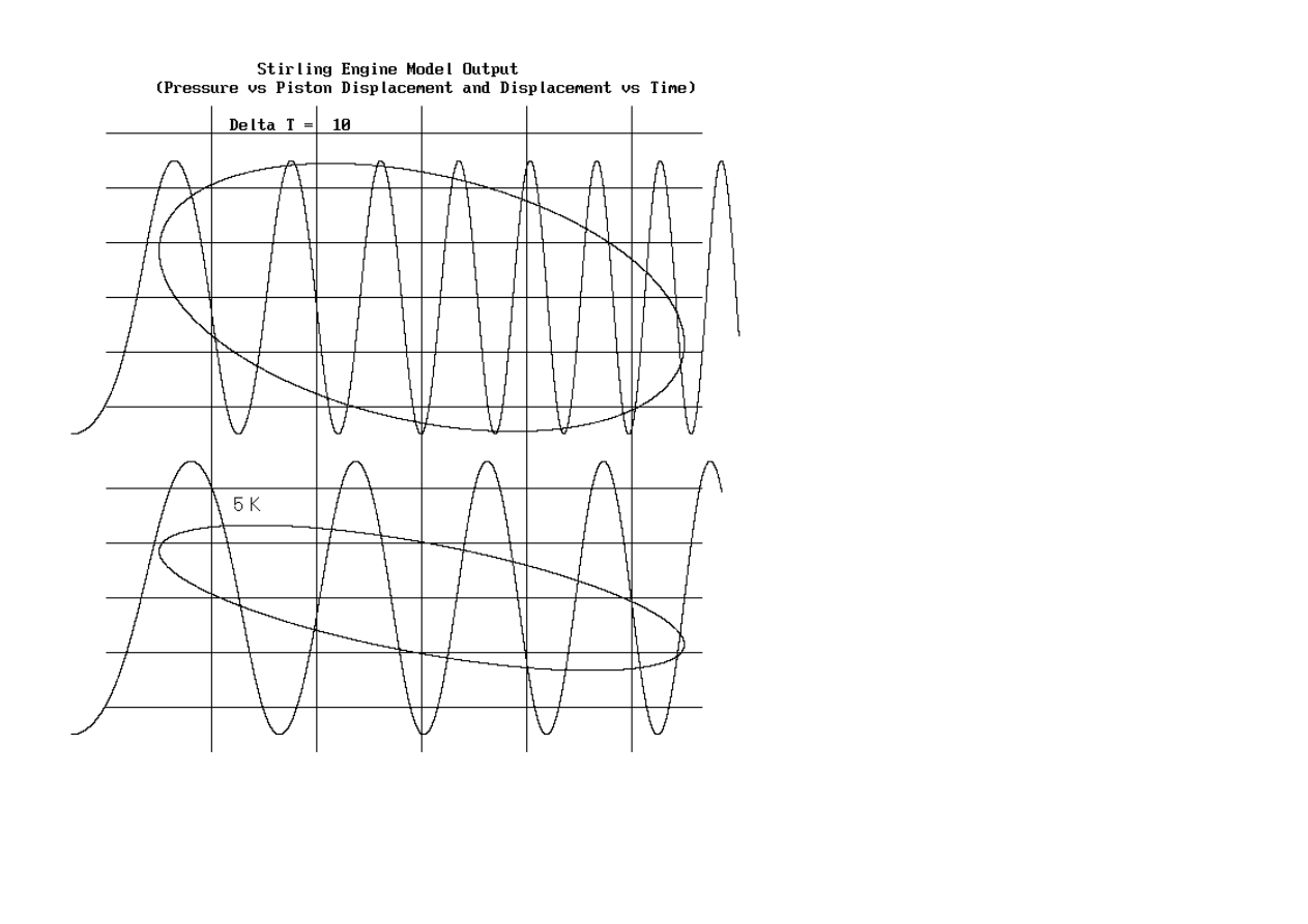
For comparison to Fig. 5, the model generated corresponding cases are shown in Fig. 6.

The Stirling Engine-Refrigerator: Rich Pedagogy from Applied Physics

http://xxx.lanl.gov/html/physics/0112061

13 sur 20

29/11/2006 11:09

Figure 6. Model generated output, two different temperature cases, each showing both hysteresis and pressure variation with time.

The scales are linear and the spacing between horizontal lines is 0.2 V and the spacing between vertical lines is 1 s for the time plots and 0.25 cm for the
hysteresis plots. The engine was initialized at

ω

= 2 rad/s and

θ

= 0.

The Stirling Engine-Refrigerator: Rich Pedagogy from Applied Physics

http://xxx.lanl.gov/html/physics/0112061

14 sur 20

29/11/2006 11:09

Q

H

= N k

⌠
⌡

T

0

+

∆

T

2

sin

θ

f -

ρ

R cos

θ

ρ

R sin

θ

d

θ

Q

H

=

N k

ρ

R

f

(2 T

0

+

π

4

∆

T)

Q

L

=

N k

ρ

R

f

( 2 T

0

-

π

4

∆

T)

W = Q

H

- Q

L

=

π

2

N k

f

ρ

R

∆

T

The observed peak-to-peak variations at 1700 Pa and 3300 Pa for the two cases differ slightly from the measured 1900 Pa and 3100 Pa respectively, but these
differences are consistent with uncertainties in the temperature.

6 Efficiency

Stirling engines have been built with efficiencies that are a significant fraction of the maximum possible value, which is that of the Carnot cycle. In the theory
which follows, it will be shown that this is true for a frictionless (ideal) Stirling engine of the type that was studied.

The efficiency is calculated by applying the first law of thermodynamics to the assumed ideal gas. As the piston moves from y = -R to y = R, heat flows into
the engine. As seen from Equations (6) and (8), these two values of y share the same temperature. Thus the heat input from the high temperature reservoir can
be calculated by integrating NkT dV/V. We rewrite the variables in terms of

θ

and integrate from 0 to

π

, letting T

0

= (T

L

+ T

H

)/2, so that T = T

0

+ 0.5×

∆

T

sin

θ

. Since the volume is V = V

0

(f -

ρ

R cos

θ

), the heat into the engine from the hot reservoir is given by

(10)

Ignoring the term

ρ

R cos

θ

<<

f, this can be readily integrated to yield

(11)

Similarly, the heat leaving the engine from the low temperature reservoir during the return path (change of

θ

from

π

to 2

π

) is given by

(12)

The work done in traversing one cycle (change of

θ

from 0 to 2

π

) is thus

(13)

Dividing Eq.(13) by Eq.(11) yields the efficiency for the frictionless (ideal) Stirling engine as presently described.

The Stirling Engine-Refrigerator: Rich Pedagogy from Applied Physics

http://xxx.lanl.gov/html/physics/0112061

15 sur 20

29/11/2006 11:09

η

= (

1

2

+

2

π

T

H

+ T

L

T

H

- T

L

)

-1

(14)

Since the efficiency of a Carnot cycle is given by 1 - T

L

/T

H

, it is seen that the present idealized Stirling engine has an efficiency of 88% that of the Carnot in

the limit T

L

<<

T

H

. At the other extreme, the efficiency becomes

η

→

π∆

T/(4T) as

∆

T

→

0.

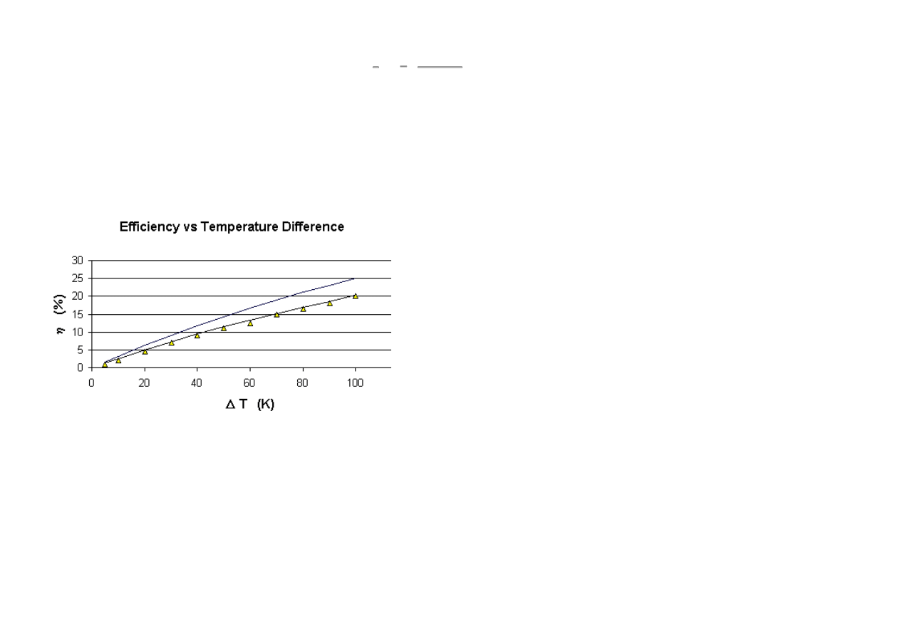
To determine the efficiency with friction included, W was obtained by using model generated data and estimating the area of the hysteresis loop of pressure
versus volume. This was done through use of the graph of P vs y, for a range of

∆

T values. The results are shown in Fig. 7, where the estimates for the engine

are denoted by the points. It is seen that friction, as modeled, does not significantly decrease the efficiency of the engine.

Figure 7. Calculated Efficiency of the Stirling engine with friction. The curve close to the calculated points is from Eq.(14). The upper curve is for the Carnot
cycle.

The data of Fig. 7 are semi-experimental, since they were obtained using output from a model that was fitted to measurements of pressure and piston
displacement. Additionally, the heat input was based on theory. Quality of the efficiency estimates could not be assessed, since no attempt was made to directly
measure the heat input and the corresponding power output from the engine. Although the latter could probably be readily measured, perhaps with a
miniaturized `prony' brake; an accurate measurement of the heat transfer is expected to be a challenge.

7 Theoretical limitations

The hysteresis curves generated by the computer are ellipses. They are a decent fit to experiment at lower operating temperatures, but the same is not true at

The Stirling Engine-Refrigerator: Rich Pedagogy from Applied Physics

http://xxx.lanl.gov/html/physics/0112061

16 sur 20

29/11/2006 11:09

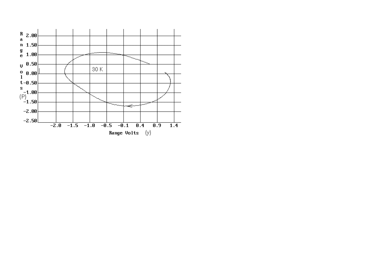
high temperatures. There is increased harmonic content in the pressure waveform, due to the turning points becoming `sharper' than predicted by theory. For
example, appreciable distortion is evident in Fig.8, which was taken with the engine operating at

∆

T = 30 K.

Figure 8. Illustration of distortion in the pressure waveform at higher temperatures. (The arrow was added to the curve to show direction of circulation.)

In generating Fig. 8, the engine was not allowed to run at full speed, limited only by its friction; this because of the frequency response limitation of the
pressure sensor. The gain of the electronics begins to significantly decline above about 2 to 3 Hz, so an external friction torque load was supplied so that the
steady state period of the flywheel was about 1 s for this case.

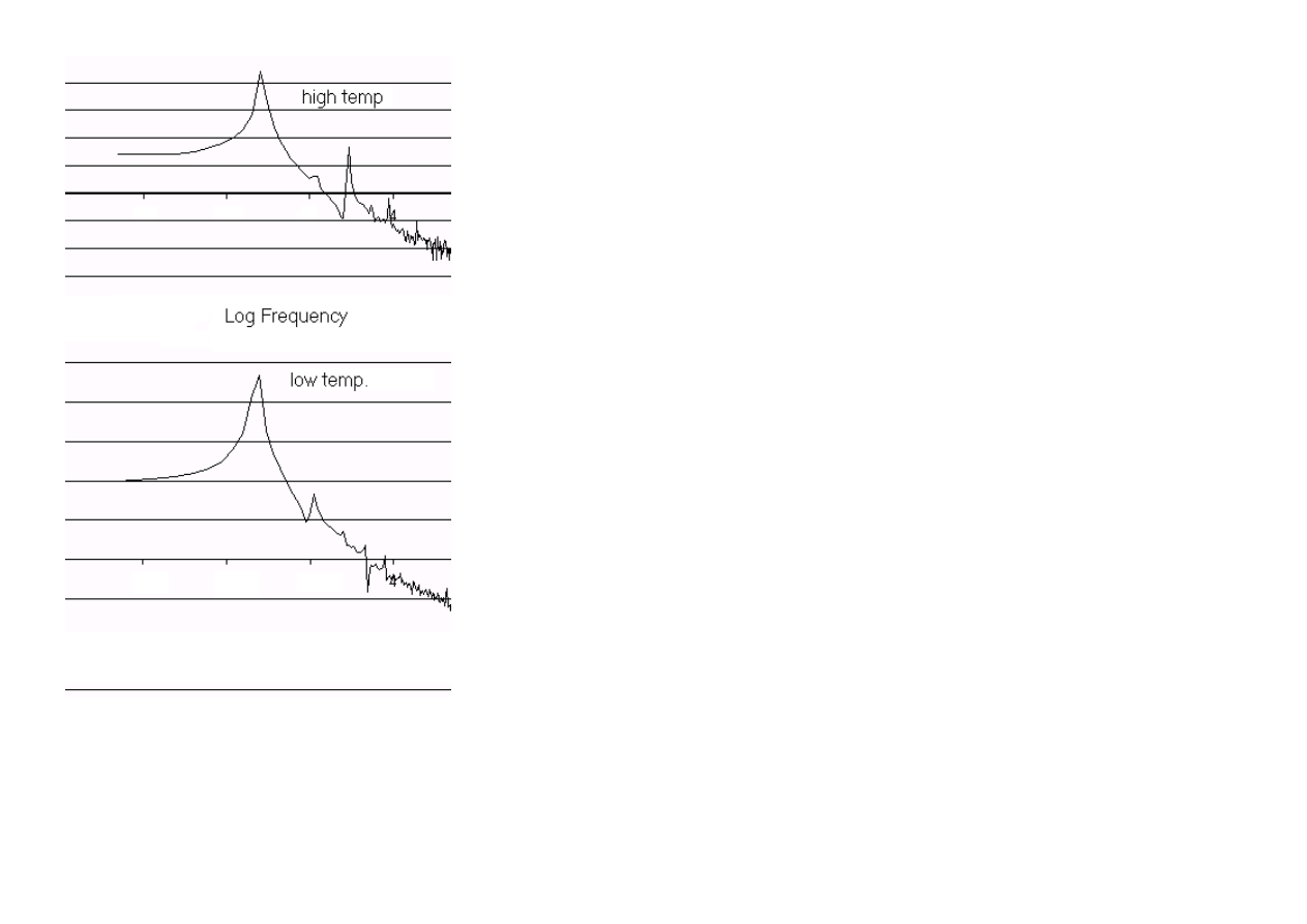
The amount of distortion is even greater when the flywheel is not constrained, with the pressure waveform taking on an increasingly sawtooth character. This
is illustrated in the pair of log-log power spectra plots of Fig. 9, where the third harmonic is seen to be significant in the high temperature case, where Delta T

≈

30 K. For the low temperature case,

∆

T

≈

10 K. These spectra were generated by (i) exporting the 512-point pressure data from KIS to Excel, (ii)

performing the FFT, and (iii) graphing the sum of the squares of the real and imaginary components of the transformed set. They are intended for comparison
only, the abscissa and ordinate axes being left purposely unlabeled.

The Stirling Engine-Refrigerator: Rich Pedagogy from Applied Physics

http://xxx.lanl.gov/html/physics/0112061

17 sur 20

29/11/2006 11:09

Figure 9. Comparison of power spectra, showing the onset of harmonic distortion as

∆

T is increased.

No attempt was made to improve agreement between theory and experiment at the higher temperatures. Nor was there any serious attempt to quantify the
importance of this theoretical deficiency. A `second-order' description of the engine, to factor in such complexities, is thought to be a daunting task.

APPENDIX

The Stirling Engine-Refrigerator: Rich Pedagogy from Applied Physics

http://xxx.lanl.gov/html/physics/0112061

18 sur 20

29/11/2006 11:09

Whirling Catheter Technique for Pressure Sensor Calibration

It can be difficult to calibrate a highly sensitive pressure sensor using the techniques that are commonly employed with higher pressure instruments.
Additionally in the case of a manometer, the fluid required for its operation is cause for inconvenience. In the whirling catheter method described here, the
only items needed to simply perform a calibration are: (i) a length of small-diameter rubber tubing about 2 m in length, (ii) a meter-stick, and (iii) a
stopwatch-along with the electronics (including meter) to indicate the output voltage of the pressure sensor.

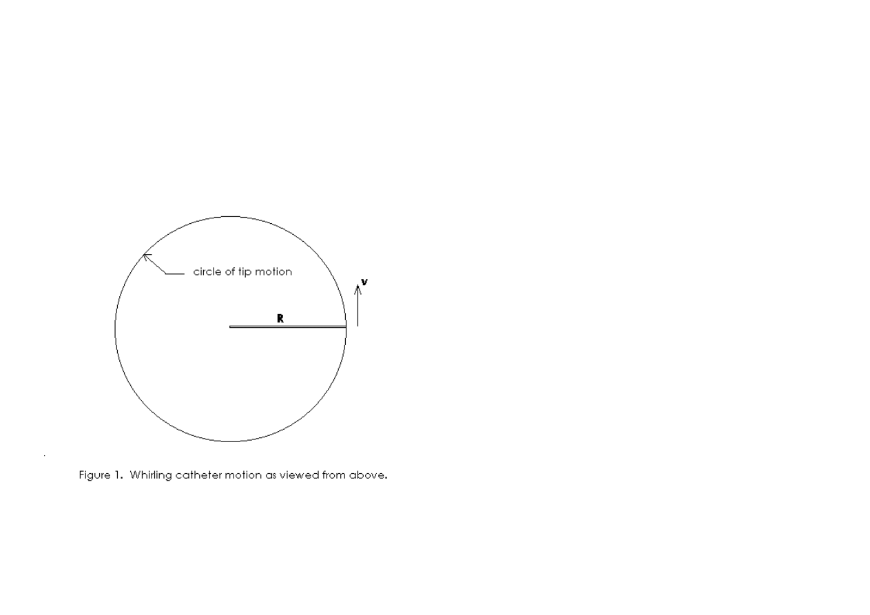
One end of the catheter is connected to the pressure sensor, which is held with one hand below the `stationary center' of the circle shown in Figure 1. The
other hand lightly holds the tubing at a distance R from the open end, which is swung in a horizontal overhead circle. The reference port of the sensor
diaphragm is open to room air, so that the instrument is operated in a differential mode.

To begin calibration, one chooses an operating radius R (such as 0.75 m); which determines the point from the open end of the tubing where it is to be grasped
between thumb and forefinger. With this point defining the ``center'' of the circle, the tubing is whirled overhead as if twirling a tethered ball. The circle's
`center' is not perfectly defined because the hand which does the swinging is not stationary, but rather moves in a small circle of its own to maintain the
motion.

The Stirling Engine-Refrigerator: Rich Pedagogy from Applied Physics

http://xxx.lanl.gov/html/physics/0112061

19 sur 20

29/11/2006 11:09

P =

1

2

ρ

v

2

The output voltage from the instrument is visually monitored- most readily by observing the needle of an analog rather than the numerals of a digital meter.
While observing the needle, the speed of the tip v is maintained at a near constant value by manually adjusting the angular rate of motion. For example, if the
voltage begins to fall slightly, then the dipping of the voltmeter needle shows that the tubing needs to be swung a little faster. With a little practice, one with
average hand-eye coordination can by this feedback arrangement maintain the voltage constant to better than 10% full-scale reading of the meter, for R in the
range from 0.5 - 1.0 m. A single observer can both control the speed of the catheter and also operate a stopwatch to measure the period of the motion. To
reduce reaction time errors, it is convenient to measure through ten rotations of the catheter, as opposed to the challenge of a single rotation.

Relationship between v and the pressure differential P

Consider a differential length of air in the tubing dr at distance r from the center of the circle. For inner tubing cross-sectional area A, the differential mass of
air contained in dr is given by

ρ

Adr; where

ρ

is the density of air. For angular rate,

ω

= v/R, the centripetal force required to hold the differential mass in

place is given by dF =

ρ

A(v

2

/R

2

)dr. Dividing this force by A yields the pressure difference between the ends of the differential mass. Integrating this

expression for the pressure difference from r = 0 to r = R yields the amount of pressure reduction from the open end of the tube to the center of the tube,
where the value of the pressure is the same as that being measured by the sensor. The result turns out to be the same as the kinetic term in Bernoulli's equation;
i.e.,

(15)

Results

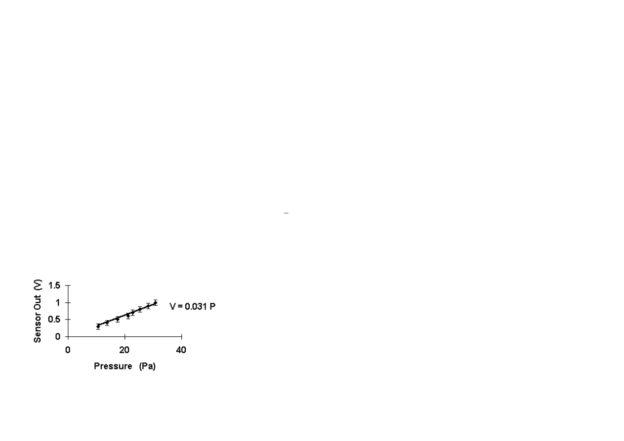
Sample results of the use of this calibration technique are shown in Figure 2, where R = 1.0 m and the density of air was set at

ρ

= 1.29 kg/m

3

.

Figure 2. Calibration data, SDC Pressure Sensor.

The Stirling Engine-Refrigerator: Rich Pedagogy from Applied Physics

http://xxx.lanl.gov/html/physics/0112061

20 sur 20

29/11/2006 11:09

The data of Fig. 2 were obtained using a pressure sensor of the type invented and patented by the author [3], which uses a thin aluminized mylar diaphragm
and a doubly differential capacitive detector arrangement.

The calibration constant in Figure 2 is seen to be 0.031 V/Pa. When used with the Stirling engine, the electronics gain had to be attenuated by approximately
100 to prevent saturation.

References
1. A. Cromer, ``Stable solutions using the Euler approximation'', Amer. J. Phys. 49, 455-457 (1981).
2. R. Peters, ``Full-bridge capacitive extensometer'', Rev. Sci. Instrum. 64(8), 2250 (1993). The extensometer of this reference has cylindrical electrodes,
whereas the sensor of the presently described study uses planar electrodes; however, they are electrically equivalent.
3. R. Peters, ``Symmetric differential capacitive pressure sensor'', Rev. Sci. Instrum. 64(8), 2256-2261 (1993).

File translated from TEX by

TTH

, version 1.95.

On 19 Dec 2001, 11:54.