Major A Spin Network Primer (1999) [sharethefiles com]

arXiv:gr-qc/9905020 v2 22 Aug 1999

A SPIN NETWORK PRIMER

SETH A. MAJOR

Abstract.

Spin networks, essentially labeled graphs, are “good quantum

numbers” for the quantum theory of geometry. These structures encompass a
diverse range of techniques which may be used in the quantum mechanics of
finite dimensional systems, gauge theory, and knot theory. Though accessible
to undergraduates, spin network techniques are buried in more complicated
formulations. In this paper a diagrammatic method, simple but rich, is intro-
duced through an association of 2

×2 matrices to diagrams. This spin network

diagrammatic method offers new perspectives on the quantum mechanics of
angular momentum, group theory, knot theory, and even quantum geometry.
Examples in each of these areas are discussed.

UWThPh - 1999 - 27

1. Introduction

Originally introduced as a quantum model of spatial geometry [1], spin networks

have recently been shown to provide both a natural home for geometric operators
[2] and a basis for the states of quantum gravity kinematics [3]. At their roots, spin
networks provide a description of the quantum mechanics of two-state systems.
Even with this humble foundation, spin networks form a remarkably diverse struc-
ture which is useful in knot theory, the quantum mechanics of angular momentum,
quantum geometry, and other areas.

Spin networks are intrinsically accessible to undergraduates, but much of the the

material is buried in more complex formulations or lies in hard-to-find manuscripts.
This article is intended to fill this gap. It presents an introduction to the diagram-
matic methods of spin networks, with an emphasis on applications in quantum
mechanics. In so doing, it offers undergraduates not only a fresh perspective on
angular momentum in quantum mechanics but also a link to leading edge research
in the study of the Hamiltonian formulation of quantum gravity. One quantum
operator of geometry is presented in detail; this is the operator which measures the
area of a surface.

The history of spin networks goes back to the early seventies when Penrose first

constructed networks as a fundamentally discrete model for three-dimensional space
[1]. Difficulties inherent in the continuum formulation of physics led Penrose to ex-
plore this possibility.

These difficulties come from both quantum and gravitational

theory as seen from three examples: First, while quantum physics is based on non-
commuting quantities, coordinates of space are commuting numbers, so it appears
that our usual notion of space conflicts with quantum mechanics. Second, on a more

Date: 20 August 1999.

There are more philosophic motivations for this model as well. Mach advocated an inter-

dependence of phenomena: “The physical space I have in mind (which already includes time) is
therefore nothing but the dependence of the phenomena on one another. A completed physics
that knew of this dependence would have no need of separate concepts of space and time because
these would already have be encompassed” [4] echoing Leibniz’s much earlier critique of Newton’s
concept of absolute space and time. Penrose invokes such a Machian principle: A background
space on which physical events unfold should not play a role; only the relationships of objects to
each other can have significance [1].

SETH A. MAJOR

pragmatic level, quantum calculations often yield divergent answers which grow ar-
bitrarily large as one calculates physical quantities on finer and smaller scales. A
good bit of machinery in quantum field theory is devoted to regulating and renor-
malizing these divergent quantities. However, many of these difficulties vanish if
a smallest size or “cut-off” is introduced. A discrete structure, such as a lattice,
provides such a cut-off. Thus, were spacetime built from a lattice or network, then
quantum field theory would be spared much of the problems of divergences. Third,
there is a hint coming from general relativity itself. Since regular initial data, say
a collapsing shell of matter, can evolve into a singularity, relativity demonstrates
that the spacetime metric is not always well-defined. This suggests that it is prof-
itable to study other methods to model spacetime. As the absolute space and time
of Newton is a useful construct to apply in many everyday calculations, perhaps
continuous spacetime is simply useful as a calculational setting for a certain regime
of physics.

Motivated by these difficulties, Penrose constructed a discrete model of space.

The goal was to build a consistent model from which classical, continuum geometry
emerged only in a limit. Together with John Moussouris he was able to show
that spin networks could reproduce the familiar 3 dimensional angles of space – a
“theory of quantized directions” [5]. In this setting, spin networks were trivalent
graphs labeled by spins.

Later, spin networks were re-discovered by Rovelli and Smolin when they were

searching for the eigenspace of operators measuring geometric quantities such as
area and volume [2], [6]. In this setting spin networks had to be generalized to
include graphs with higher valence vertices. This early work launched many stud-
ies which resulted in a powerful suite of spin network techniques for background-
independent quantization.

Spin networks are fantastically useful both as a basis for the states of quantum

geometry and as a computational tool.

Spin network techniques were used to

compute the spectrum of area [6] and volume [7] operators. Spin networks, first
used as a combinatorial basis for spacetime, find application in quantum gravity,
knot theory, and group theory.

This spin network primer begins by associating 2

×2 matrices with diagrams. The

first goal is to make the diagrammatics “planar isotopic,” meaning the diagrams
are invariant under smooth deformations of lines in the plane. It is analogous to
the manipulations which one would expect for ordinary strings on a table. Once
this is completed, the structure is enriched in Section 2.3 to allow combinations
and intersections between lines. This yields a structure which includes the rules
of addition of angular momentum. It is further explored in Section 3 with the
diagrammatics of the usual angular momentum relations of quantum mechanics.
(A reader more familiar with the angular momentum states of quantum mechanics
may wish to go directly to this section to see how spin networks are employed in
this setting.) In Section 4 this connection to angular momentum is used to give
a diagrammatic version of the Wigner-Eckart theorem. The article finishes with a
discussion on the area operator of quantum gravity.

2. A play on line

This section begins by building an association between the Kronecker delta func-

tions the 2

× 2 identity matrix (or δ

) and a line. It is not hard to ensure that the

lines behave like elastic strings on a table. The association and this requirement
leads to a little bit of knot theory, to the full structure of spin networks, and to a
diagrammatic method for the quantum mechanics of angular momentum.

A SPIN NETWORK PRIMER

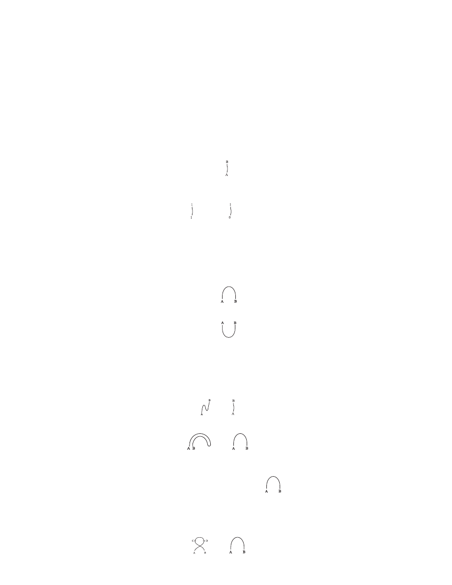
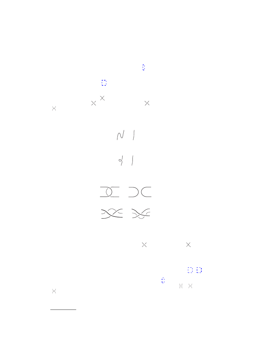
2.1. Line, bend and loop. The Kronecker δ

is the 2

× 2 identity matrix in

component notation. Thus,

and δ

= δ

= 1 while δ

= δ

= 0. The Latin capital indices, A and B in

this expression, may take one of two values 0 or 1. The diagrammatics begins by
associating the Kronecker δ to a line

∼

The position of the indices on δ determines the location of the labels on the ends
of the line. Applying the definitions one has

= 1 and

= 0.

If a line is the identity then it is reasonable to associate a curve to a matrix with

two upper (or lower) indices. There is some freedom in the choice of this object.
As a promising possibility, one can choose the antisymmetric matrix

(

) =

−1 0

so that

∼

Similarly,

∼

As a bent line is a straight line “with one index lowered” this choice fits well with
the diagrammatics: δ

After a bit of experimentation with these identifications, one discovers two awk-

ward features. The diagrams do not match the expected moves of elastic strings in
a plane. First, since δ

−δ

, straightening a line yields a

negative sign:

− .

(1)

Second, as a consequence of

−

(2)

However, these “topological” difficulties are fixed by modifying the definition of a
bent line. One can add an i to the antisymmetric tensors

→ ˜

= i

so that ˜

Since each of the two awkward features contains a pair of ’s the i fixes these sign
problems. However, there is one more property to investigate.

On account of the relation δ

−˜

one has (The indices C and D are

added to the diagram for clarity.)

−

SETH A. MAJOR

– not what one would expect for strings.

This final problem can be cured by

associating a minus sign to each crossing.

Thus, by associating an i to every and a sign to every crossing, the diagrams

behave as continuously deformed lines in a plane [1]. The more precise name of
this concept is known as planar isotopy. Structures which can be moved about
in this way are called topological. What this association of curves to δ’s and ˜

’s

accomplishes is that it allows one to perform algebraic calculations by moving lines
in a plane.

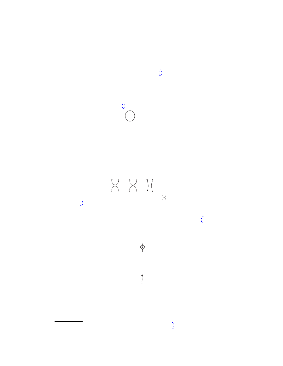
A number of properties follow from the above definitions. The value of a simple

closed loop takes a negative value

−2,

(3)

since ˜

−

−2; a closed line is a number. This turns out to be

a generic result in that a spin network which has no open lines is equivalent to a
number.

A surprisingly rich structure emerges when crossings, are considered. For in-

stance the identity, often called the “spinor identity,” links a pair of epsilons to
products of deltas

= δ

− δ

Using the definitions of the ˜

matrices one may show that, diagrammatically, this

becomes

= 0.

(4)

Note that the sign changes, e.g.

−δ

becomes +

. This diagrammatic rela-

tion of Eq. (4) is known as “skein relations” or the “binor identity.” The utility of
the relation becomes evident when one realizes that the equation may be applied
anywhere within a larger diagram.

One can also decorate the structure by “weighting” or “tagging” edges.

Instead

of confining the diagrams to simply be a sum of products of δ’s and ’s, one can
include other objects with a tag. For instance, one can associate a tagged line to
any 2

× 2 matrix such as ψ

B
A

∼

These tags prove to be useful notation for angular momentum operators and for the
spin networks of quantum geometry. Objects with only one index, can frequently
be represented as Kronecker delta functions with only one index. For example,

The result of these associations is a topological structure in which algebraic

manipulations of δ’s, ’s, and other 2

× 2 matrices are encoded in manipulations of

open or closed lines. For instance, straightening a wiggle is the same as simplifying
a product of two ˜

’s to a single δ. It also turns out that the algebra is “topological:”

Any two equivalent algebraic expressions are represented by two diagrams which can
be continuously transformed into each other. Making use of a result of Reidemeister

This led Penrose to dub these “negative dimensional tensors” [1]. In general relativity, the

dimension of a space is given by the trace of the metric, g

µν

, hence the name.

There is some redundancy in notation. Numerical (or more general) labels associated to edges

are frequently called weights or labels. The term “tag” encompasses the meaning of these labels
as well as operators on lines.

A SPIN NETWORK PRIMER

and the identities above it is a few lines of δ-algebra to show that the spin network
diagrammatics is topologically invariant in a plane.

2.2. Reidemeister Moves. Remarkably, a knot

in three dimensional space can

be continuously deformed into another knot, if and only if, the planar projection of
the knots can be transformed into each other via a sequence of four moves called
the “Reidemeister moves” [10]. Though the topic of this primer is mainly on two
dimensional diagrams, the Reidemeister moves are given here in their full generality
– as projections of knots in three dimensional space. While in two dimensions one
has only an intersection,

, when two lines cross, in three dimensions one has

the “over crossing,”

and the “undercross,”

, as well as the intersection

There are four moves:

• Move 0: In the plane of projection, one can make smooth deformations of

the curve

∼

• Move I: As these moves are designed for one dimensional objects, a curl may

be undone

∼

This move does not work on garden-variety string. The string becomes twisted
(or untwisted). (In fact, this is the way yarn is made.)

• Move II: The overlaps of distinct curves are not knotted

∼

• Move III: One can perform planar deformations under (or over) a diagram

∼

With a finite sequence of these moves the projection of a knot may be transformed
into the projection of any other knot which is topologically equivalent to the origi-
nal. If two knots may be expressed as the other with a sequence of these moves then
the knots are called “isotopic.” Planar isotopy is generated by all four moves with
the significant caveat that there are no crossings

, only intersections

. Pla-

nar isotopy may be summarized as the manipulations one would expect for elastic,
non-sticky strings on a table top – if they are infinitely thin.

Move I on real strings introduces a twist in the string. This move is violated by

any line which has some spatial extent in the transverse direction such as ribbons.
Happily, there are diagrammatic spin networks for these “ribbons” as well [11], [12].

2.3. Weaving and joining. The skein relations of Eq. (4) show that, given a
pair of lines there is one linear relation among the three quantities:

, and

. So a set of graphs may satisfy many linear relations. It would be nice to

select a basis which is independent of this identity. After some work, this may be
accomplished by choosing the antisymmetric combinations of the lines – “weaving

A mathematical knot is a knotted, closed loop. One often encounters collections of, possibly

knotted, knots. These are called links.

SETH A. MAJOR

with a sign.”

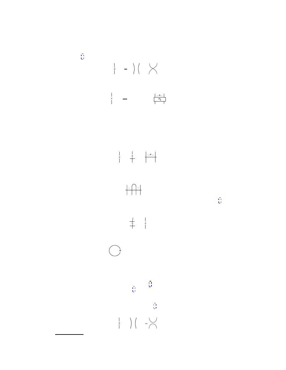
The simplest example is for two lines

1
2

−

(5)

For more than two lines the idea is the same. One sums over permutations of the
lines, adding a sign for each crossing. The general definition is

∈S

(

−1)

|σ|

(6)

in which a σ represents one permutation of the n lines and

|σ| is the minimum

number of crossings for this permutation. The boxed σ in the diagram represents
the action of the permutation on the lines. It can be drawn by writing 1 2 . . . n,
then permutation just above it, and connecting the same elements by lines.

In this definition, the label n superimposed on the edge record the number of

“strands” in the edge. Edge are usually labeled this way, though I will leave simple
1-lines unlabeled. Two other notations are used for this weaving with a sign

These antisymmetrizers have a couple of lovely properties, retacing and pro-

jection: The antisymmetrizers are “irreducible,” or vanish when a pair of lines is
retraced

= 0.

(7)

which follows from the antisymmetry. Using this and the binor identity of Eq. (4)
one may show that the antisymmetrizers are “projectors” (the combination of two
is equal to one)

Making the simplest closed diagram out of these lines gives the loop value often

denoted as ∆

= ∆

= (

−1)

(n + 1).

The factor n + 1 expresses the “multiplicity” of the number of possible “A-values”
on an edge with n strands. Each line in the edge carries an index, which takes two
possible values. To see this note that for an edge with a strands the sum of the
indices A, B, C, ... is 0, 1, 2, ..., a. So that the sum takes a + 1 possible values. One
may show using the recursion relations for ∆

that the loop value is equal to this

multiplicity. As we will see in Section 3 the number of possible combinations is the
dimension of the representation.

As an example of the loop value, the 2-loop, has value 3. This is easily checked

using the relations for the basic loop value (Eq. (3)) and the expansion of the 2-line
using the skein relation

1
2

(8)

Note that, because of the additional sign associated to crossings, the “antisymmetrizer” sym-

metrizes the indices in the δ world.

The loop value satisfies ∆

= 1, ∆

−2, and ∆

n+2

= (

−2)∆

n+1

− ∆

A SPIN NETWORK PRIMER

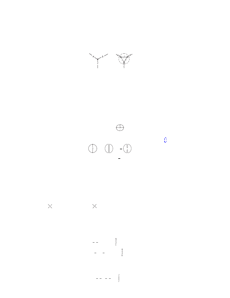
Edges may be further joined into networks by making use of internal trivalent

vertices

The dashed circle is a magnification of the dot in the diagram on the left. Such
dashed curves indicate spin network structure at a point. The “internal” labels
i, j, k are positive integers determined by the external labels a, b, c via

i = (a + c

− b)/2, j = (b + c − a)/2, and k = (a + b − c)/2.

As in quantum mechanics the external labels must satisfy the triangle inequalities

a + b

≥ c, b + c ≥ a, a + c ≥ b

and the sum a + b + c is an even integer. The necessity of these relations can be
seen by drawing the strands through the vertex.

With this vertex one can construct many more complex networks. After the

loop, the next simplest closed graph has two vertices,

θ(a, b, c) =

The general evaluation, given in the appendix, of this diagram is significantly more
complicated. As an example I give the evaluation of θ(1, 2, 1) using Eq. (8),

1
2

= (

−2)

(

−2) = 3.

One can build ever more complicated networks. In fact, one can soon land a dizzying
array of networks. I have collected a small zoo in the appendix with full definitions.

Now all the elements are in place for the definition of spin networks. A spin

network consist of a graph, with edges and vertices, and labels. The labels, asso-
ciated edges, represent the number of strands woven into edges. Any vertex with
more than three incident edges must also be labeled to specify a decomposition into
trivalent vertices. The graphs of spin networks need not be confined to a plane.
In a projection of a spin network embedded in space, the crossings which appear
in the projection may be shown as in the Reidemeister moves with over-crossing
“

” and under-crossing “

”.

3. Angular momentum representation

As spin networks are woven from strands which take two values, it is well-suited

to represent two-state systems. It is perhaps not surprising that the diagrammatics
of spin networks include the familiar

| jmi representation of angular momentum.

The notations are related as

1
2

i = u

∼

and

1
2

−

1
2

i = d

∼

(Secretly, the “u” for “up” tell us that the index A only takes the value 1. Likewise
“d” tells us the index is 0.) The inner product is given by linking upper and lower
indices, for instance

1
2

i ∼

= 1.

SETH A. MAJOR

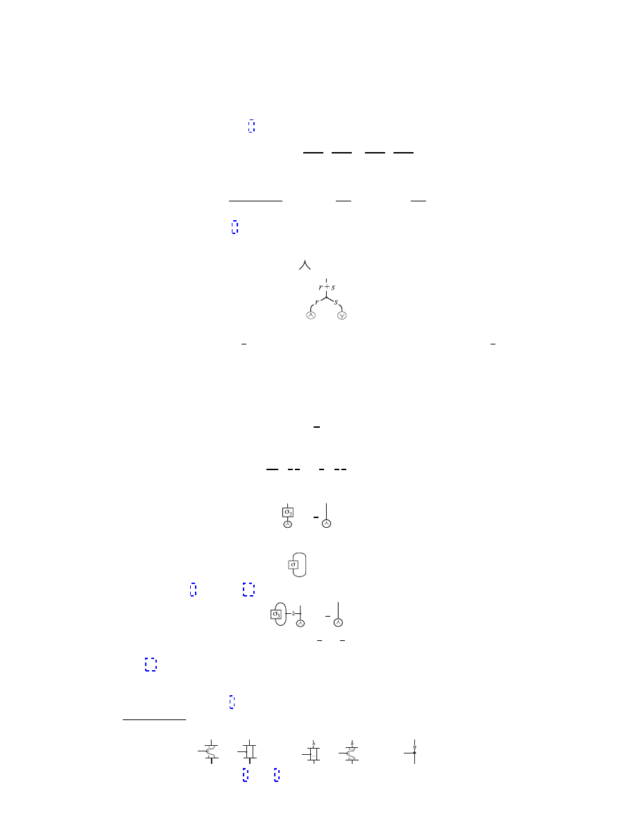
For higher representations [5]

| j mi :=| r si = N

. . . u

}

. . . d

F )

}

(9)

in which

r! s! (r + s)!

1/2

, j =

r+s

, and m =

−s

(10)

The parentheses in Eq. (9) around the indices indicate symmetrization, e.g. u

+ u

. The normalization N

ensures that the states are orthonormal in

the usual inner product. A useful representation of this state is in terms of the
trivalent vertex. Using the notation “

” for u and similarly for d I have

| j mi ∼

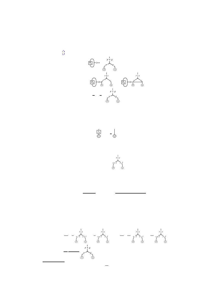
Angular momentum operators also take a diagrammatic form. As all spin net-

works are built from spin-

1
2

states, it is worth exploring this territory first. Spin-

1
2

operators have a representation in terms of the Pauli matrices

, σ

−i

, σ

−1

with

~
2

for i = 1, 2, 3. One has

1
2

i =

1
2

which is expressed diagrammatically as

1
2

Or, since Pauli matrices are traceless,

= 0,

and using Eq (8) one has [14]

1
2

A similar relation holds for the states

1
2

−

1
2

i. The basic action of the spin

operators can be described as a “hand” which acts on the state by “grasping” a
line [13]. The result, after using the diagrammatic algebra, is either a multiple of
the same state, as for σ

, or a new state. If the operator acts on more than one

line, a higher dimensional representation, then the total action is the sum of the
graspings on each edge.

This may be shown by noticing that

, so that

· · · = n

as may be derived using Eqs. (4) and (7).

A SPIN NETWORK PRIMER

The ˆ

operator can be constructed out of the σ

matrix. The total angular

momentum z-component is the sum of individual measurements on each of the
sub-systems.

In diagrams, the action of the ˆ

operator becomes

| j mi ∼

= r

+ s

−

≡ ~ m | j mi.

The definition of the quantities r and s was used in the last line.

This same procedure works for the other angular momentum operators as well.

The ˆ

operator is constructed from the Pauli matrix σ

. When acting on one line

the operator ˆ

matrix “flips the spin” and leaves a factor

1
2

The reader is encouraged to try the same procedure for ˆ

The raising and lowering operators are constructed with these diagrams as in

the usual algebra. For the raising operator ˆ

= ˆ

+ i ˆ

one has

| j mi ∼ ~s

In a similar way one can compute

−

| j mi = ~

(r + 1)s

| j mi

from which one can compute the normalization of these operators: Taking the inner
product with

hj m | gives the usual normalization for the raising operator

| j mi = ~

s(r + 1)

| j mi = ~

− m)(j + m + 1) | j mi.

Note that since r and s are non-negative and no larger than 2j, the usual condition
on m,

−j ≤ m ≤ j, is automatically satisfied.

Though a bit more involved, the same procedure goes through for the ˆ

opera-

tor. It is built from the sum of products of operators ˆ

= ˆ

+ ˆ

. Acting

once with the appropriate Pauli operators, one finds

| j mi ∼ ~









 + ~






−






(r + s)

The operator is ˆ

2j+1
i=1

⊗ ... ⊗

⊗ ... ⊗ 1 where the sum is over the possible

positions of the Pauli matrix.

SETH A. MAJOR

Acting once again, some happy cancellation occurs and the result is

| j mi =

+ s

+ rs + r + s

| j mi

which equals the familiar j(j + 1). Actually, there is a pretty identity which gives
another route to this result. The Pauli matrices satisfy [14]

1
2

i=1

B
i A

D
i C

(11)

so the product is a 2-line. Similarly, the ˆ

operator may be expressed as a 2-line.

As will be shown in Section 5 this simplifies the above calculation considerably.

4. A bit of group theory

As we have seen, spin networks, inspired by expressing simple δ and matrices

in terms of diagrams, are closely related to the familiar angular momentum repre-
sentation of quantum mechanics. This section makes a brief excursion into group
theory to exhibit two results which take a clear diagrammatic form, Schur’s Lemma
and the Wigner-Eckart Theorem.

Readers with experience with some group theory may have noticed that spin

network edges are closely related to the irreducible representations of SU (2). The
key difference is that, on account of the sign conventions chosen in Section 2.1, the
usual symmetrization of representations is replaced by the antisymmetrization of
Eq. (6). In fact, each edge of the spin network is an irreducible representation.
The tags on the edges can identify how these are generated – through the spatial
dependence of a phase, for instance.

Since this diagrammatic algebra is designed to handle the combinations of ir-

reducible representations, all the familiar results of representation theory have a
diagrammatic form. For instance, Schur’s Lemma states that any matrix T which
commutes with two (inequivalent) irreducible representations D

and D

of dimen-

sions a + 1 and b + 1 is either zero or a multiple of the identity matrix

T D

= D

T for all g

∈ G =⇒ T =

(

if a

6= b

if a = b

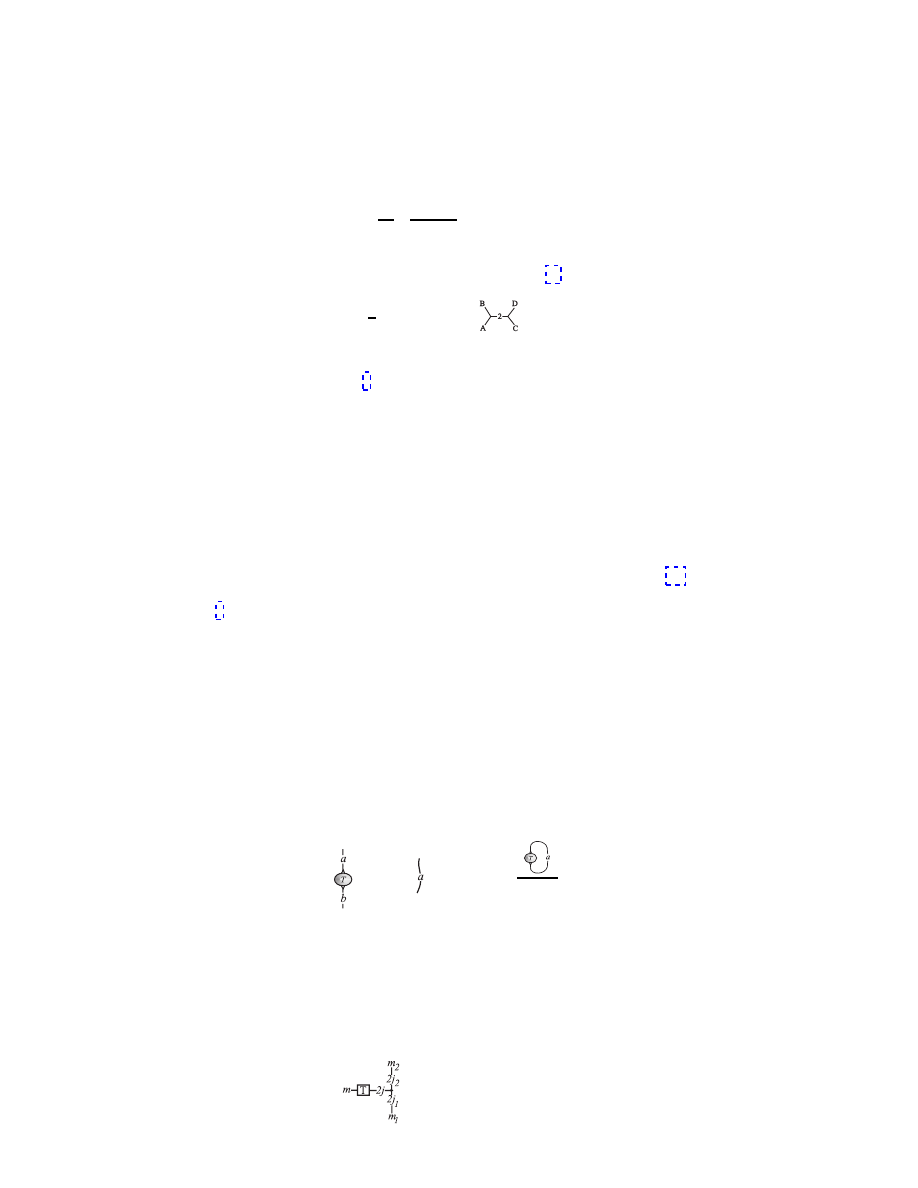
Diagrammatically, this is represented as

= λ δ

, where λ =

∆

The constant of proportionality is given by λ which, being a closed diagram, eval-
uates to a number.

The Wigner-Eckart theorem also takes a nice form in the diagrammatic language,

providing an intuitive and fresh perspective on the theorem. It can help those
who feel lost in the mire of irreducible tensor operators, reduced matrix elements,
and Clebsch-Gordon coefficients. A general operator T

grasping a line in the j

representation (2j

lines) to give a j

representation is expressed as

∼ hj

| T

| j

A SPIN NETWORK PRIMER

Just from this diagram and the properties of the trivalent vertex, it is already clear
that

− j

| ≤ j ≤ j

+ j

Likewise it is also the case that

= m

+ m.

These results are the useful “selection rules” which are often given as a corollary to
the Wigner-Eckart theorem. Notice that the operator expression is a diagram with
the three legs j, j

, and j

. This suggests that it might be possible to express the

operator as a multiple of the basic trivalent vertex.

Defining

one can combine the two lower legs together with Eq. (21). Applying Schur’s
Lemma, one finds

j+j

|j−j

∆

θ(2j, 2j

, c)

= ω

(12)

where

ω =

θ(2j, 2j

, 2j

)

This relation expresses the operator in terms of a multiple of the trivalent vertex.
It also gives a computable expression of the multiplicative factor. Comparing the
first and last terms with the usual form of the theorem –

| T

| j

i = hj

| |T

| | j

ihjmj

| j

– one can immediately see that the reduced matrix element

| |T

| | j

i is the ω

of Eq. (12). In this manner, any invariant tensor may be represented as a labeled,
trivalent graph.

5. Quantum Geometry: Area operator

In this final example of the spin network diagrammatic algebra, the spectrum

of the area operator of quantum gravity is derived. Before beginning, I ought to
remark that the hard work of defining what is meant by the quantum area operator
is not done here. The presentation instead concentrates on the calculation of the
spectrum.

There are many approaches to constructing a quantum theory of gravity. The

plethora of ideas arises in part from the lack of experimental guidance and in part
from the completely new setting of general relativity for the techniques of quanti-
zation. One promising direction arises out of an effort to construct a background-
independent theory which meets the requirements of quantum mechanics. This
field may be called “loop quantum gravity” or “spinet gravity.” (See Ref. [19] for
a recent review.) The key idea in this approach is to lay aside the perturbative
methods usually employed and, instead, directly quantize the Hamiltonian theory.

Since the Clebsch-Gordan symbols are complete, any map from a

⊗ b to c must be a multiple

of the Clebsch-Gordan or 3j-symbol.

See, for instance, Reference [15] pg. 573 or Reference [16] pg. 116.

SETH A. MAJOR

Recently this field has bloomed. There is now a mathematically rigorous under-
standing of the kinematics of the theory and a number of (in principle testable)
predictions of quantum geometry. One of the intriguing results of this study of
quantum geometry is the discrete nature of space.

In general relativity the degrees of freedom are encoded in the metric on space-

time. However, it is quite useful to use new variables to quantize the theory [17].
Instead of a metric, in the canonical approach the variables are an “electric field,”
which is the “square root” of the spatial metric, and a vector potential. The elec-
tric field E is not only vector but also takes 2

× 2 matrix values in an “internal”

space. This electric field is closely related to the coordinate transformation from
curved to flat coordinates (a triad). The canonically conjugate A, usually taken to
be the configuration variable, is similar to the electric vector potential but is more
appropriately called a “matrix potential” for A also is matrix valued. It determines
the effects of geometry on spin-

1
2

particles as they are moved through space.

(See

Refs. [18] and [19] for more on the new variables.) States of loop quantum gravity
are functions of the potential A. A convenient basis is built from kets

| si labeled

by spin networks s. In this application of spin networks, they have special tags or
weights on the edges of the graph. Every strand e of the gravitational spin network
has the “phase” associated to it.

An orientation along every edge helps to deter-

mine these phases or weights. The states of quantum geometry are encoded in the
knottedness and connectivity of the spin networks.

In classically gravity the area of a surface S is the integral

√

in which g is the determinant of the metric on the surface.

The calculation

simplifies if the surface is specified by z = 0 in an adapted coordinate system.
Expressed in terms of E, the area of a surface S only depends on the z-vector
component [6] - [9]

· E

(13)

The dot product is in the “internal” space. It is the same product between Pauli
matrices as appears in Eq. (11). In the spin network basis E is the momentum
operator. As p

→ −i~

in quantum mechanics, the electric field analogously

becomes a “hand,” E

→ −i~κ

. The τ is proportional to a Pauli matrix,

τ =

σ. The κ factor is a sign: It is positive when the orientations on the edge

and surface are the same, negative when the edge is oriented oppositely from the
surface, and vanishes when the edges is tangent to the surface. The E operator
acts like the angular momentum operator ˆ

J . Since the E operator vanishes unless

it grasps an edge, the operator only acts where the spin network intersects the
surface.

For those readers familiar with general relativity the potential determines the parallel trans-

port of spin-

particles.

In more detail, every edge has a “holonomy.”

or path ordered exponential (i.e.

P exp

dt ˙

e(t)

· A(e(t))) associated to it. See, for example, Ref. [18].

The flavor of such an additional dependence is already familiar in flat space intergrals in

spherical coordinates:

A =

sin(θ)dφdθ.

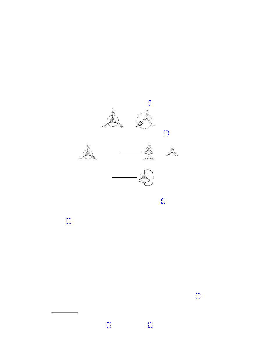
A SPIN NETWORK PRIMER

(a.)

(b.)

Figure 1.

Two types of intersections of a spin network with a

surface (a.) One isolated edge e intersects the surface transversely.
The normal ˆ

n is also shown. (b.) One vertex of a spin network lies

in the surface. All the non-tangent edges contribute to the area.
Note that the network can be knotted.

The square of the area operator is calculated first. Calling the square of the

integrand of Eq. (13) ˆ

O, the two-handed operator at one intersection is

| si = −

· ˆ

| si

(14)

where the sum is over edges e

at the intersection. Here, ˆ

denotes the vector

operator ˆ

J = ˆ

+ ˆ

acting on the edge e

. This ˆ

O is almost ˆ

but for the

sign factors κ

. The area operator is the sum over contributions from all parts of the

spin network which thread through the surface. In terms of ˆ

O over all intersections

| si =

1/2

| si,

including the dimensional constants.

As a first step, one can calculate the action of the operator ˆ

O on an edge e

labeled by n as depicted in Figure 13(a.). In this case, the hands act on the same
edge so the sign is 1, κ

= 1, and the angle operator squared becomes proportional

to ˆ

! In the calculation one may make use of the Pauli matrix identity of Eq. (11)

| si = − ˆ

| si

−~

| (s − e)i.

The edge is shown in the the diagram so it is removed spin network s giving the
state

| (s − e)i. Now the diagram may be reduced using the recoupling identities.

The bubble may be extracted with Eq. (18)

| si = −~

| (s − e)i

−~

θ(n, n, 2)

∆

| (s − e)i

−~

−

n + 2

| si

n(n + 2)

| si,

SETH A. MAJOR

in which Eq. (17) was also used in the second line. Putting this result into the area
operator, one learns that the area coming from all the transverse edges is [6]

| si =

+ 2)

| si

= l

2
P

+ 1)

| si.

(15)

The units

~, c, and G are collected into the Planck length l

∼ 10

−35

The result is also re-expressed in terms of the more familiar angular momentum
variables j =

The full spectrum of the area operator is found by considering all the intersections

of the spin network with the surface S including vertices which lie on the surface
as in Figure 13(b.). Summing over all contributions [8]

| si =

2
P

+ 1) + 2j

+ 1)

− j

+ 1)

1/2

| si

in which j

) is the total spin with a positive (negative) sign κ and j

is the

total spin of edges tangent to the surface at the vertex v.

This result is utterly remarkable in that the calculation predicts that space is

discrete. Measurements of area can only take these quantized values. As is the
case in many quantum systems there is a “jump” from the lowest possible non-zero
value. This “area quanta” is

√

. In an analogous fashion, as for an electron in a

hydrogen atom, surfaces make a quantum jump between states in the spectrum of
the area operator.

6. Summary

This introduction to spin networks diagrammatics offers a view of the diversity

of this structure. Touching on knot theory, group theory, and quantum gravity this
review gives a glimpse of the applications. These techniques also offer a new per-
spective on familiar angular momentum representations of undergraduate quantum
mechanics. As shown with the area operator in the last section, it is these same
techniques which are a focus of frontier research in the Hamiltonian quantization
of the gravitational field.

Acknowledgment. It is a pleasure to thank Franz Hinterleitner and Johnathan
Thornburg for comments on a draft of the primer. I gratefully acknowledge support
of the FWF through a Lise Meitner Fellowship.

Appendix

A. Loops, Thetas, Tets and all that

This appendix contains the basic definitions and formulae of diagrammatic re-

coupling theory using the conventions of Kauffman and Lins [12] – a book written
in the context of the more general Temperley-Lieb algebra .

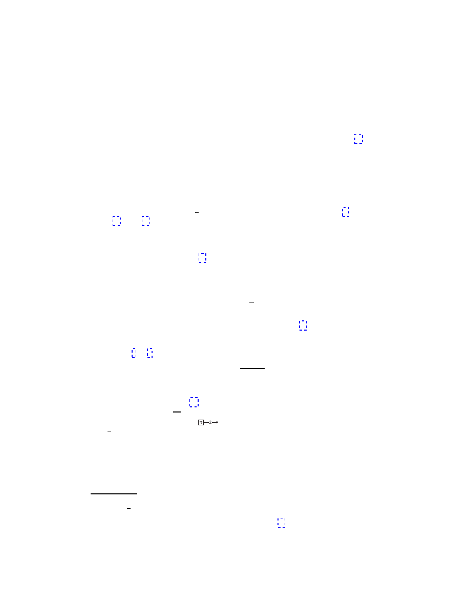
The function θ(m, n, l) is given by

θ(m, n, l) =

= (

−1)

(a+b+c)

(a + b + c + 1)!a!b!c!

(a + b)!(b + c)!(a + c)!

(16)

where a = (l + m

− n)/2, b = (m + n − l)/2, and c = (n + l − m)/2. An evaluation

which is useful in calculating the spectrum of the area operator is θ(n, n, 2), for
which a = 1, b = n

− 1, and c = 1.

θ(n, n, 2) = (

−1)

(n+1)

(n + 2)! (n

− 1)!

(2n!)

= (

−1)

(n+1)

(n + 2)(n + 1)

(17)

A SPIN NETWORK PRIMER

A “bubble” diagram is proportional to a single edge.

= δ

(

−1)

θ(a, b, n)

(n + 1)

(18)

The basic recoupling identity relates the different ways in which three angular

momenta, say a, b, and c, can couple to form a fourth one, d. The two possible
recouplings are related by

i’

|a−b|≤i≤(a+b)

(19)

where on the right hand side is the 6j-symbol defined below. It is closely related
to the T et symbol. This is defined by [12]

= T et

T et

= N

≤s≤S

(

−1)

(s + 1)!

− a

− s)!

N =

i,j

− a

a!b!c!d!e!f!

(20)

in which

1
2

(a + d + e)

1
2

(b + d + e + f)

1
2

(b + c + e)

1
2

(a + c + e + f)

1
2

(a + b + f)

1
2

(a + b + c + d)

1
2

(c + d + f)

m = max

} M = min {b

}

The 6j-symbol is then defined as

T et

∆

θ(a, d, i) θ(b, c, i)

These satisfy a number of properties including the orthogonal identity

= δ

and the Biedenharn-Elliot or Pentagon identity

Two lines may be joined via

∆

θ(a, b, c)

(21)

One also has occasion to use the coefficient of the “λ-move”

= λ

ab
c

where λ

ab
c

= (

−1)

−c

]/2

(22)

SETH A. MAJOR

References

[1] Roger Penrose, “Angular momentum: An approach to combinatorial spacetime” in

Quantum Theory and Beyond T. Bastin, ed. (Cambridge University Press, Cambridge,
1971); “Combinatorial Quantum Theory and Quantized Directions” in Advances in
Twistor Theory, Research Notes in Mathematics 37, L. P. Hughston and R. S. Ward,
eds. (Pitman, San Francisco, 1979) pp. 301-307; “Theory of Quantized Directions,” un-
published notes.

[2] Carlo Rovelli and Lee Smolin, ”Spin Networks and Quantum Gravity,” Phys. Rev. D 52

5743-5759 (1995).

[3] John C. Baez, “Spin networks in gauge theory,” Advances in Mathematics 117 253

- 272 (1996), Online Preprint Archive: http://xxx.lanl.gov/abs/gr-qc/9411007; “Spin
Networks in Nonperturbative Quantum Gravity,” in The Interface of Knots and Physics,
Louis Kauffman, ed. (American Mathematical Society, Providence, Rhode Island, 1996),
pp. 167 - 203, Online Preprint Archive: http://xxx.lanl.gov/abs/gr-qc/9504036.

[4] Ernst Mach, Fichtes Zeitschrift f¨

ur Philosophie 49 227 (1866). Cited in Lee Smolin in

Conceptual Problems of Quantum Gravity, A. Ashtekar and J. Stachel, eds. (Birkh¨

auser,

Boston, 1991).

[5] John P. Moussouris, “Quantum models as spacetime based on recoupling theory,” Oxford

Ph.D. dissertation, unpublished (1983).

[6] Carlo Rovelli and Lee Smolin, “Discreteness of area and volume in quantum gravity,”

Nuc. Phys. B 442, 593-622 (1995).

[7] Roberto De Pietri and Carlo Rovelli, “Geometry eigenvalues and the scalar product from

recoupling theory in loop quantum gravity,” Phys. Rev. D 54(4), 2664-2690 (1996).

[8] Abhay Ashtekar and Jerzy Lewandowski, “Quantum Theory of Geometry I: Area oper-

ators,” Class. Quant. Grav. 14, A55-A81 (1997).

[9] S. Fittelli, L. Lehner, C. Rovelli, “The complete spectrum of the area from recoupling

theory in loop quantum gravity,” Class. Quant. Grav. 13, 2921-2932 (1996).

[10] K. Reidemeister, Knotentheorie (Chelsea Publishing Co., New York, 1948), original

printing (Springer, Berlin, 1932). See also Louis Kauffman, Knots and Physics, pp. 16.

[11] Louis H. Kauffman, Knots and Physics, Series on Knots and Everything - Vol. 1 (World

Scientific, Singapore, 1991) pp. 125-130, 443-471.

[12] Louis H. Kauffman and S´

ostenes L. Lins, Temperley-Lieb Recoupling Theory and In-

variants of 3-Manifolds, Annals of Mathematics Studies N. 134, (Princeton University
Press, Princeton, 1994), pp. 1-100.

[13] Carlo Rovelli and Lee Smolin, “Loop Representation of quantum general relativity,” Nuc.

Phys. B 331(1), 80-152 (1990).

[14] R. DePietri, “On the relation between the connection and the loop representation of

quantum gravity,” Class. Quant. Grav. 14 53-70 (1990).

[15] Albert Messiah, Quantum Mechanics, Vol. 2 (John Wiley, New York, 1966).
[16] H.F. Jones, Groups, Representations and Physics (Adam Hilger, Bristol, 1990).
[17] Abhay Ashtekar, “New variables for classical and quantum gravity,” Phys. Rev. Lett.

57(18), 2244-2247 (1986); New perspectives in canonical gravity (Bibliopolis, Naples,
1988); Lectures on non-perturbative canonical gravity, Advanced Series in Astrophysics
and Cosmology-Vol. 6 (World Scientific, Singapore, 1991).

[18] Abhay

Ashtekar,

“Quantum

mechanics

Riemannian

geometry,”

http://vishnu.nirvana.phys.psu.edu/riem qm/riem qm.html.

[19] Carlo

Rovelli,

“Loop

Quantum

Gravity,”

Living

Reviews

Relativity

http://www.livingreviews.org/Articles/Volume1/1998-1rovelli;

“Strings, Loops,

and

Others: A critical survey of the present approaches to quantum gravity,” in Grav-
itation and Relativity:

At the turn of the Millennium, Proceedings of the GR-15

Conference, Naresh Dadhich and Jayant Narlikar, ed. (Inter-University Center for
Astronomy and Astrophysics, Pune, India, 1998), pp. 281 - 331, Online Preprint
Archive: http://xxx.lanl.gov/abs/gr-qc/9803024.

Institut f¨

ur Theoretische Physik, Der Universit¨

at Wien, Boltzmanngasse 5, A-1090

Wien AUSTRIA

E-mail address : smajor@galileo.thp.univie.ac.at