First Order Digital Filters--An Audio Cookbook

Application Note AN-11 by Christopher Moore

Introduction
The simplest digital filters are first order FIR and IIR filters,
singly or in cascade. While not as powerful as higher order fil-
ters, they are nevertheless of considerable interest in audio for
bass and treble controls, DC offset removal, high pass filters,
and low pass filters. Also appealing is the low computational
burden that first order filters place on DSP resources.
Despite the simplicity of the first order filter, the DSP literature
is not forthcoming with a simple methodology that allows for
cookbook design. The method that I present here appears in an
article from 1978 by Ham and is based on relating a prototype
analog filter to the desired digital filter using the technique of
impulse invariance. See Mitra (1998), pages 425-431, for further
information on this technique.
The system function of a first order discrete time filter is:

1

2

1

2

1

1

)

(

−

−

−

+

=

z

a

z

b

b

z

H

Using the technique of impulse invariance, one ends up with
exponential functions that let you map from the continuous time
filter’s corner frequencies directly to the coefficients of the dis-
crete time (digital) filter.
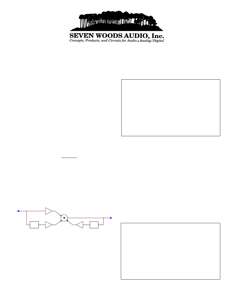
The flow chart of a first order digital filter (Direct Form 1
structure) is shown below. Other structures, while yielding the
same response, may be advantageous in some cases due to finite
word length and other effects.

z-1

b1

X(n)

b2

Y(n)

a2

z-1

a2 is the coefficient of the pole feedback path. A plus sign in the
tables indicates that the feedback path has a positive gain. If you
are using the Matlab freqz function, you must enter -a2 to satisfy
its sign convention for poles. The coefficient a1 is not shown on
the flow chart as it relates to the gain of the output itself, which
is always one.
To actually implement one of these filters, you will need a DSP
environment in which to program a chip to carry out the indi-
cated sample storage, multiplication, and accumulation.

Assembly language example (not optimized)

Motorola 56002

;

Low pass 1

st

order filter

move

X:fsum,x0

; source sample into x0

move

Y:B_1,y0

; filter coef into y0

mpy

x0,y0,

a Y:B_2,y1 ; mpy source sample,

; get next coef

move

X:sumz0,x1

; get z-1 delayed source
: sample into x1

move

x0,X:sumz0

; update delayed source

mac

x1,y1,a

Y:A_2,y1 ; mac 2nd sum term,

; get next coef

move

x:intz0,x1

; get z-1 output into x1

macr

y1,x1,a

; macr 3rd and final term

move

a,X:intz0

; update z-1 out register

move

a,X:fsum

; update output

The values of b1 and b2 shown in the tables are simplified initial
values, but the normalization factor norm was used in the freqz
evaluation. Normalization was set to give unity gain at either DC
or Fn, as appropriate. The normalization factor can be further
modified according to signal dynamic range requirements. To
incorporate normalization, scale b1 and b2 through multiplica-
tion by norm.
Each filter type is illustrated with a Matlab plot showing the
digital filter response computed using Matlab’s freqz function.
Generally, the digital filter matches the prototype analog filter
quite closely. However, at corner frequencies above about a
quarter of the Nyquist frequency (5.6kHz here), the computed
actual corner frequency begins to lag behind the target. Fur-
thermore, as the signal frequency approaches Fn, the response of
some of the filters deviates from the analog version by a few dB.
Generally, the discrepancy can be ameliorated by the appropri-
ate activation of a pole or zero of around +/-0.12.

Definitions of Terms

Fs (sampling rate) = 44.1kHz here, but can be any value
z

-1

(unit delay of sampling) = 1/Fs, seconds

Fn (Nyquist rate) = Fs/2, 22.05kHz
f: frequency, Hz
f1,f2: filter corner frequency, Hz
a1, a2, b1, b2: coefficients of the system function
abs(): absolute value function
e (base of natural logarithms) = 2.718..
zero location: -b2/b1
pole location: a2

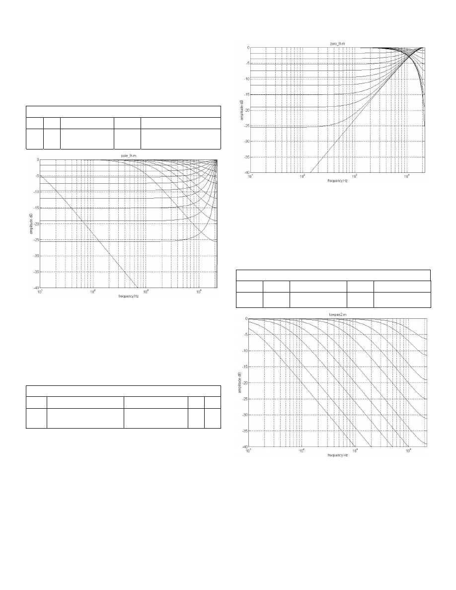
Pole
The first order pole by itself is capable of either low pass or high
pass responses, as can be seen below. The low pass curves look
potentially useful, but, by themselves, the high pass curves don’t
do much until pretty high frequencies. The high pass curves will
come in handy to lift curves where the zero response doesn’t
quite behave.

Pole (POLE_LH.M)

b

1

b

2

norm

a

1

a

2

1

0

1/(1-abs(a2))

1

varied from 0 to +/-

0.999 in steps of 0.1

Zero
The first order zero by itself is also capable of either low pass or
high pass responses. The high pass curves look potentially use-
ful, but, by themselves, the low pass curves don’t do much until
pretty high frequencies. The low pass curves will come in handy
to pull down curves where the pole response doesn’t quite be-
have. It is very hard to look at these curves and deduce how to
choose pole and zero responses that together will yield the de-
sired filter.

Zero (ZERO_LH.M)

b

1

b

2

norm

a

1

a

2

-1

varied from 0 to

+/-1.0 in steps of 0.1

abs(b1)+abs(b2)

1

0

Low Pass Filter
The low pass filter utilizes only the feedback portion of the filter
to realize a pole that sets f1, the corner frequency, appropriately.
In the curves below, f1 was set to 10, 20, 50, 100, 200, 500, 1k,
2k, 5k, and 10kHz. By enabling a zero at -0.12, you can add the
extra attenuation needed to more closely match the continuous
time filter at 10kHz and above. Furthermore, if additional roll
off is required in the range of 4kHz and higher, the zero can be
set even to -1.0, which gives zero output at Fn.

Low Pass (LOWPAS2.M)

b

1

b

2

norm

a

1

a

2

1.0

0.12

(1-a2)/(b1+b2)

1

N

F

f

e

/

1

π

−

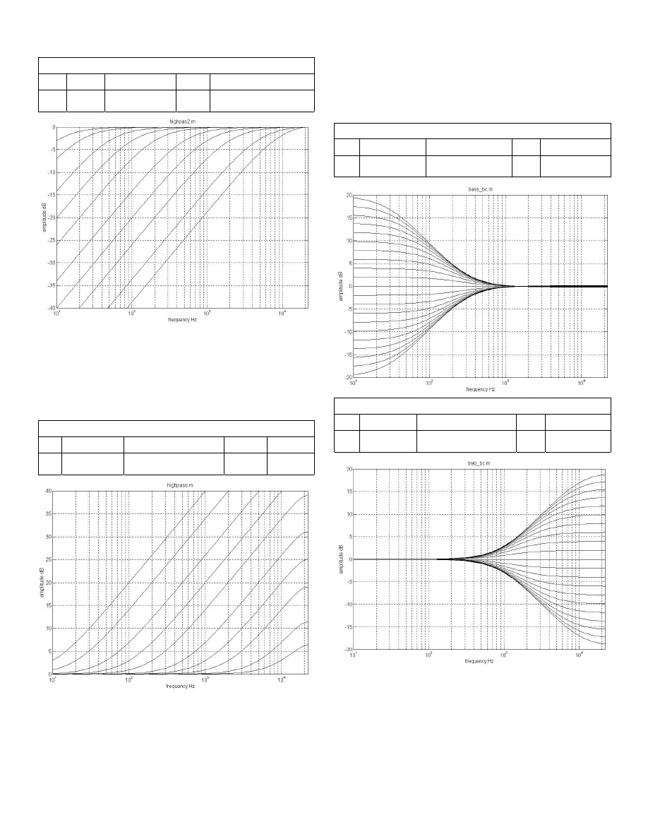
High Pass Filter
The high pass filter utilizes the feed forward portion of the filter
to realize a zero at DC and the feedback portion to create a pole
that pulls the rising response down to a flat response. The re-
sponse rises from zero at DC to a shelf at f1. This characteristic
is useful for DC offset removal filters. In the curve below, f1
was set to 10, 20, 50, 100, 200, 500, 1k, 2k, 5k, and 10kHz.

High Pass (HIGHPAS2.M)

b

1

b

2

norm

a

1

a

2

1

-1

(1+a2)/2

1

N

F

f

e

/

1

π

−

High Pass Filter with Low Frequency Shelf
The high pass filter utilizes only the feed forward portion of the
filter to realize a shelf at low frequencies. The response begins
rising off the shelf at f2. In the curves below, f2 was set to 10,
20, 50, 100, 200, 500, 1k, 2k, 5k, and 10kHz. By enabling a
pole at -0.12, you can add the extra gain needed to more closely
match the continuous time filter at 10kHz and above.

High Pass (HIGHPASS.M)

b

1

b

2

norm

a

1

a

2

-1

N

F

f

e

/

2

π

−

(1-a2)/abs(b1+b2)

1

-0.12

Shelf (bass, treble)
The shelf filter utilizes both feed forward and feed back sec-
tions. If f1 < f2, output falls from higher to lower level with in-
creasing frequency, and response is suitable for bass boost or
treble cut. If f2 < f1, output rises from lower to higher level with
increasing frequency, and response is suitable for bass cut or
treble boost. Shelf level difference is dB(f1/f2). In the bass and

treble graphs below, one corner frequency was fixed (300Hz for
the bass control and 1kHz for the treble control) and the other
corner frequency was varied in log spaced steps over a range of
10:1. The Matlab file for the treble control is given on the last
page.

Shelf (BASS_BC.M)

b

1

b

2

norm

a

1

a

2

-1

N

F

f

e

/

2

π

−

1

1

N

F

f

e

/

1

π

−

−

Shelf (TREB_BC.M)

b

1

b

2

norm

a

1

a

2

-1

N

F

f

e

/

2

π

−

(1-a2)/(b1+b2)

1

N

F

f

e

/

1

π

−

Design notes
Even though the expressions used to compute the coefficients
are quite simple, the computation should be mechanized if more
than a few curves are required. I used Matlab, creating multiple
files, one for each of the graphs seen here (the file names are
shown in parantheses), but MathCAD or even a spreadsheet
could also be used.

Example Matlab file, TREB_BC.M

%TREB_BC.M Creates treble control with corner fre-
quency at 1kHz and sweeps from -20dB to +20dB in 20
steps
%
% revision date: March 3, 2001
%
% constants
Fs=44100;

% sampling rate

t=1/Fs;

% sampling interval

Fn=Fs/2;

% Nyquist frequency

minF=10;

% minimum frequency of analysis

maxF=Fs/2;

% maximum frequency of analysis

numPts=256;

% number of points of analysis

%
% create array of frequencies to use for freqz
Farray=logspace(log10(minF),log10(maxF),numPts);
%
% create arrays of frequencies in Hz to use for
sweeping the treble control
Fcarray1=[ 1000 1258 1584 1995 2512 3162 3981 5011
6310 7943 10000 1000 1000 1000 1000 1000 1000
1000 1000 1000 1000 ];
Fcarray2=[ 1000 1000 1000 1000 1000 1000 1000 1000
1000 1000 1000 1258 1584 1995 2512 3162 3981
5011 6310 7943 10000 ];
%
clf;

% clear graph

for A_index = 1: 21

% plot 21 times for 2dB steps

of boost and cut over +/- 20dB range
%
title ('treb_bc.m');

% do every iteration to get

correct appearance
xlabel ('frequency Hz');
ylabel ('amplitude dB');
axis([minF maxF -20 20 ]);
grid on;
%
f2=Fcarray2(A_index);

% numerator (zero) freq

f1=Fcarray1(A_index); % denominator (pole) freq
%
%-------------------------------------------------
% compute the digital filter coefficients
%
L1= exp(-pi*f2/Fn); % numerator
K1= exp(-pi*f1/Fn); % denominator
%
b1=-1,

%numerator coefficient X(n)

b2= L1,

%numerator coefficient X(n-1)

a1= 1,

%denominator coefficient Y(n)

a2= K1,

%denominator coefficient Y(n-1)

normalize=(1-a2)/(b1+b2);

% normalize to AV=0dB at

DC
b1=normalize*b1;
b2=normalize*b2;
%
%define numerator and denominator of transfer func-
tion
num=[ b1 b2 ], den=[ a1 -a2 ],
% num=[ Xn Xn-1 ], den=[ Yn Yn-1 ],
%
% fill array H with transfer function amplitude
[H,W]=freqz(num,den,Farray,Fs);
%
% plot digital filter magnitude response, log in x,
linear in dB in y
semilogx(Farray,20*log10(H),'w');
hold on; % Hold plot from prior to next case
%
end

% A_index loop

In conclusion—
Although I’ve presented a variety of equalization and filter
curves here, the world of first order filters offers still more pos-
sibilities. The zero and the pole each can be located in two pos-
sible regions: between zero and +1 (DC), and between zero and
-1 (Nyquist frequency). This gives four possible combinations,
and, since there are an infinite number of possible locations,
many more curves are possible.
Acknowledgements
I would like to thank the reviewers of this application note for
their helpful suggestions--Professor Douglas Preis, Tufts Uni-
versity; Erik Anderson; Dave Tweed; and Roman Litovsky.

Bibliography
Ham, P. A. L. “Simple Digital Filters,” Wireless World, July
1978, p 83-87.
McClellan, James H., Shaver, Ronald W., and Yoder, Mark A.
DSP First: A Multimedia Approach, Prentice Hall, NJ, 1998.
Mitra, Sanjit K. Digital Signal Processing--A Computer-Based
Approach, McGraw-Hill, New York, 1998.
Orfanidis, Sophocles J. Introduction to Signal Processing,
Prentice Hall, NJ, 1996.

Mission statement of Seven Woods Audio
I am an electrical engineering consultant specializing in the con-
ception and design of products and circuits used in audio appli-
cations. My company, Seven Woods Audio, is committed to
helping manufacturers quickly create digital or analog audio
products that generate a good return on investment, work right
the first time, sound excellent, and please the end user. Seven
Woods Audio works with manufacturers of professional audio,
consumer audio, broadcast, telecommunications, and computer
equipment.

rev: March 3, 2001 Copyright 2001. All rights reserved.

44 Oak Avenue Belmont, MA 02478-2715 USA

voice/fax [phone]

[e-mail]

http://www.world.std.com/~cmoore/