Copyright 2002 AADE Technical Conference

This paper was prepared for presentation at the AADE 2002 Technology Conference “Drilling & Completion Fluids and Waste Management”, held at the Radisson Astrodome
Houston, Texas, April 2 - 3, 2002 in Houston, Texas. This conference was hosted by the Houston Chapter of the American Association of Drilling Engineers. The information presented in this paper does
not reflect any position, claim or endorsement made or implied by the American Association of Drilling Engineers, their officers or members. Questions concerning the content of this paper should be
directed to the individuals listed as author/s of this work.

Abstract
The occurrence of barite sag has been a well
recognized, but poorly understood phenomenon in the
drilling industry. Often the conditions under which barite
sag is measured in laboratory tests are unrelated to the
field conditions under which barite sag occurs. Dynamic
barite sag is now recognized as the major contributor to
sag-related drilling problems and focus on static sag has
rightfully diminished. Dynamic sag is best measured
and studied with a flow loop designed to mirror field
conditions such as annular flow rates, angle, eccentricity
and, to a degree, temperature. Time and manpower
resources required to perform flow loop tests are
significant and limit the extent to which they are
conducted.

Dynamic barite sag is a very complex process that is

often difficult to measure, predict and manage. There
are two prominent variables conducive to creating
dynamic sag; 1) insufficient ultra-low shear rate viscosity
(mud-related) and 2) low shear rate conditions (drilling-
related). Contrary to common belief, dynamic sag is not
entirely a mud-related problem and, under certain
conditions, can occur despite appropriate control of
drilling fluid viscosity. This paper reviews traditional
and newly emerging technology to measure and predict
dynamic barite sag. It also reviews the effects of drilling
processes on dynamic sag with supporting case history
data.

Introduction
Barite sag usually is observed when circulating bottoms-
up after the mud column has been static, such as when
tripping pipe. Historically it has been associated with a
static field environment; consequently test devices and
rheological measurements were originally based on
static conditions.

1,2,3

In a departure from conventional methodology,

Hanson et al.

4

found that barite sag is most problematic

under dynamic, not static, conditions. An important
conclusion from this work was that barite sag generally
observed in the field is primarily due to barite deposition
occurring under dynamic conditions. Building upon this
work Bern et al.

5

induced barite sag by circulating at low

flow rates with an eccentric drill pipe in flow loop tests.

Rotation of the drill pipe tended to prevent bed formation
and to aid in the removal of beds. The barite sag
tendency of some muds tested was so great that they
observed the beds “avalanching” (slumping down the
test section and being incorporated back within the
system) at low flow rates.

Using a flow loop device and invert-emulsion muds

from ongoing field operations Dye

6,7

et al.

concluded that

severe dynamic sag occurs in eccentric annuli at annular
shear rates below 4 s

-1

. A new field viscometer,

capable of measuring shear viscosity at shear rates as
low as 0.0017 s

-1

, was used to measure shear viscosity

in this critical shear rate region. Dynamic sag tests and
rotational viscometer measurements were made at
equivalent shear rates and used to develop a technology
that predicts flow loop results from simple viscometer
measurements. In addition, certain findings from this
study matched earlier work by Bern et al.

8

showing the

influence of drilling variables on barite sag. These
studies found that the potential for dynamic sag:

•

is promoted by an eccentric, stationary pipe such
as when sliding in deviated wells,

•

increases under low shear rate conditions such
as when operating at a nominal annular velocity
below 100 feet/minute,

•

is not influenced by mud weight, and

•

is compounded by increased hole angle.

Barite sag is typically attributed to the mud system

and the traditional approach to manage barite sag is to
increase rheological properties of the mud system.
These efforts are often frustrating because; 1) the
proposed solution is ineffective, 2) the solution creates a
new problem such as ECD management and 3)
expectations are not met. This paper proposes that
dynamic sag is related to both the mud system and
drilling operation and these two variables cannot be
treated independently from one another. Recognition of
each variable’s influence will help define an appropriate
course of action, align expectations and facilitate better
management of barite sag.

Mud Variables Effecting Barite Sag
Important advances in understanding the origin and

AADE–02-DFWM-HO-12

New Technology to Manage Barite Sag

William Dye and Greg Mullen, Baker Hughes INTEQ Drilling Fluids

2

W. DYE, G. MULLEN

AADE–02-DFWM-HO-12

mechanisms of dynamic sag have occurred from flow
loop studies, however these devices are not well suited
for routine use. Flow loop tests require a significant
investment in time and manpower resources, which
makes them impractical for most situations. More
conventional and simplistic techniques have been
developed to fill this void, the designs of which tend
towards practical as opposed to technical attributes.
The more simplistic tests are designed for rapid analysis
and generally are equally suited for field and laboratory
use.

This paper will compare technology used to quantify

dynamic sag and present data suggesting that one
should balance practical considerations with the value
and relevance of information derived from simple tests.
In addition, a new predictive technology is proposed to
bridge the gap and balance the technical attributes of
flow loop tests with the practical merits of simplistic tests.

Flow loop tests
Flow loop tests can model field conditions such as
annular flow, hole angle and eccentricity, and serve as
the benchmark for characterizing dynamic sag under
laboratory conditions. The flow loop device shown in
Figure 1 has been used to study the relationship
between shear rate and dynamic sag using invert-
emulsion mud systems in a deviated, eccentric annulus.

6

An eccentric-wellbore hydraulics model was used to

calculate flow rates needed to induce specific shear
rates beneath the eccentric pipe. Inputs into the model
include pipe geometry, flow rate, eccentricity and
coefficients of the Herschel-Bulkley rheological model.
In most cases flow rates used provided annular shear
rates in the range of 10 to 0.06 s

-1

. Fluids were

circulated for 30 minutes at each flow rate. Typically,
four to five tests were performed on a fluid, with each
test being made at a progressively lower flow rate. The
majority of tests were performed at an angle of 60

°

,

since past studies have shown this difficult for sag
management.

6, 8

A few tests were performed at 45

°

for

comparison against data collected at 60

°

. An operating

procedure is listed in the Appendix.

Flow loop testing was conducted concurrently with

field operations, presenting a unique opportunity to
correlate laboratory and field results. Typically, values of
average dynamic sag less than 1.0 lbm/gal in flow loop
tests correspond to fluids

not having barite sag-related

problems in the field. Similarly, fluids having barite sag-
related problems in the field show a tendency towards
average dynamic sag levels above 1.0 lbm/gal in flow
loop tests.

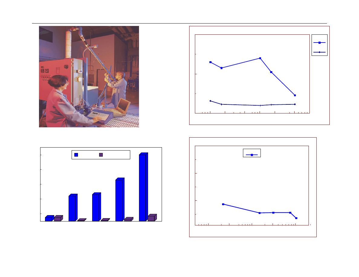
Figure 2 shows a comparison of annular shear rates

calculated in a 12 ¼” hole section when circulating at
848 US gallons per minute, assuming concentric and 50
% eccentric annuli. Hole angles in this S-shaped
trajectory varied from 67.5

°

in the 12 ¼” open hole

opposite 5” drill pipe, to about 44

°

opposite 8” drill

collars. Annular shear rates calculated for the eccentric
annulus range from 0.4 to 3.4 s

-1

, which are significantly

lower than the concentric case. Shear rates modeled in
flow loop tests realistically mirror those encountered in
actual drilling operations.

The following case histories establish correlation

between flow loop and field results. Trends in flow loop
test data correlate well with field observations of barite
sag although the absolute value of barite sag in flow loop
tests should not be directly compared to field results.

Case History No. 1 Attempts to run 9 5/8” casing to

total depth failed and casing became stuck
approximately 500 feet off bottom.

Severe dynamic sag

was observed when washing down inside of casing with
a synthetic-based mud system. Mud weight variations
measured at the rig-site when circulating bottoms-up
ranged from 12.6 to 17.4 lbm/gal, compared to a nominal
mud weight of 14.4 lbm/gal (~

∆

MW 2.4 lbm/gal).

6

This

mud was then treated with an organophilic clay-based
rheological modifier the rig-site, after previously treating
and re-testing on the flow loop, and, subsequently only
modest variations (

∆

MW 0.5 lbm/gal) were measured on

bottoms-up. Figure 3 presents flow loop test data on the
sample after being treated with a rheological modifier at
the rig-site. Flow loop tests compared favorably with field
results.

Case History No. 2 The operator repeatedly battled

lost circulation in the 12 ¼” section prior to running 9 5/8”
casing on this well drilled with a synthetic-based mud
system. The mud weight change measured on
bottoms-up after circulating on top of lost circulation
material (LCM) pills was approximately 0.8 lbm/gal.
Dynamic sag measured in the flow loop over a range of
flow rates varied from 0.36 to 0.87 lbm/gal (Figure 4).
Mud weight variations observed in the field were not
associated with the lost return problems experienced in
this section.

Case History No. 3 A sample of synthetic-based

mud was taken after completion of the 8 ½” section and
prior to running a 7” liner. Dynamic sag measured on
the flow loop ranged from 0.50 to 0.67 lbm/gal (Figure
5). The maximum differential in mud weight noted while
circulating on a wiper trip before running the liner was
0.75 lbm/gal and subsequently the liner was run and
cemented without problems. Reports from the field
indicated there were no problems associated with barite
sag.

Modified rotational viscometer test
The rotational viscometer test (RVT) is a simplistic test
used to characterize dynamic barite sag under
laboratory and field conditions.

9

The RVT utilizes the

measuring geometry of the standard 6-speed viscometer
to impart shear at a fixed rate. When rotating at 100

AADE–02-DFWM-HO-12

New Technology to Manage Barite Sag

3

rpm, the shear rate between the outer rotating sleeve
and inner bob is

≅

170 s

-1

. Dynamic sag is quantified as

the change in mud weight after rotating at 100 rpm for 30
minutes. The value of 100 rpm corresponded to
maximum sag measured in initial tests and was thought
to approximate annular shear rates at which barite sag
occurred. Practical considerations governed the choice
of 30-minute test duration.

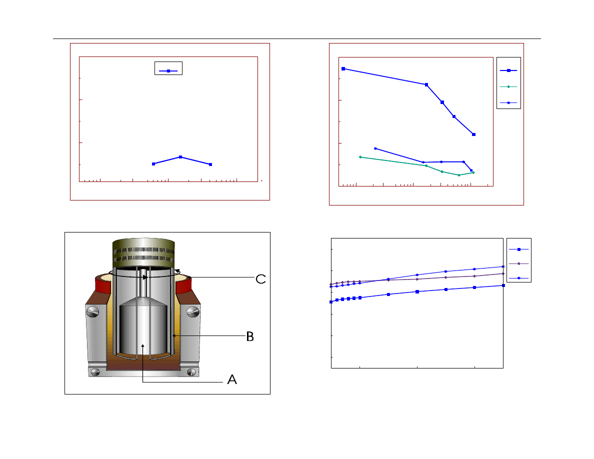
Figure 6 shows that there are actually two sets of

concentric cylinders in the RVT: the rotating sleeve/inner
bob (A-B) and the outer wall of heat cup/inner rotating
sleeve (B-C).

7

Using the dimensions of the heat cup,

sleeve and bob the shear rate between the concentric
cylinders can be calculated and expressed as a function
of the rotational speed of the viscometer. From
equation (1) the average shear rate acting across the
sleeve and bob geometry is

≅

1.7 x rpm, while the

average shear rate between the heat cup & sleeve is

≅

0.39 x rpm.

D

D

D

I

O

O

x

rpm

2

2

2

−

×

=

•

15

π

γ

(1)

Fluid volume within the sleeve/bob geometry is

≅

10

cm³ and

≅

117 cm³ between the sleeve/heat cup

geometry. This equates to a

≈

10-fold difference in

volume outside, compared to inside of the rotating
sleeve. Therefore, the RVT has two distinct fluid
volumes experiencing different shear rates, making it
difficult to determine which are contributing to the
measured result.

Modifications were made to the original RVT design

to allow for continual density and temperature
measurements. Changes included flow ports at the
bottom of the heating cup, a peristaltic pump to circulate
fluid and a densiometer to measure density and
temperature of the circulated fluid. Density and
temperature measurements are made at 1-minute
intervals for 5 minutes, followed by 5-minute intervals for
the remaining test duration (25 minutes).

Comparison of dynamic sag technologies
Dynamic sag was quantified on three invert-emulsion
muds using the flow loop and RVT. Figure 7 shows the
relationship between shear rate and dynamic barite sag
for each of these fluids measured in flow loop tests.
Generally, the magnitude of dynamic barite sag
increased as shear rate decreased below the 3-rpm
equivalent. Flow loop results shown in Figure 7
indicate that Mud #1 has the highest potential for
dynamic barite sag.

Figure 8 shows density change versus time for these

same fluids measured on the RVT at the standard
setting of 100 rpm. RVT data suggest that Mud #3 has
the highest potential for dynamic sag. A comparison of

the levels of dynamic barite sag measured on the flow
loop and the RVT appears in Table 1. Severe dynamic
sag observed in flow loop tests with Mud #1 was not
apparent using the modified RVT at the standard setting
of 100 rpm.

Significant differences are apparent when comparing

the geometry and flow paths of the flow loop and RVT.
Bern et al.

5,8

and Dye et al.

6

showed that barite sag is

most problematic when angle is greater than 30° and
generally increases with increasing hole angle. Pipe
eccentricity and low annular velocity further exacerbate
dynamic sag. The influence of critical parameters such
as hole angle, eccentricity and annular velocity on
dynamic sag cannot be delineated using the RVT.

Predictive dynamic sag technology
A new and simplistic technology is available that
correlates well with flow loop results. This technology
was derived from flow loop tests using analytical, not
empirical, techniques. Dynamic sag and rotational
viscosity were measured at equivalent shear rates and a
relationship between the two exists such that one can
predict flow loop results using viscometer
measurements. This technology possesses the
technical relevance of flow loop tests but is simpler and
less time-consuming to perform. In most cases this
technology is used instead of flow loop tests, which
makes it uniquely suited for offshore use.

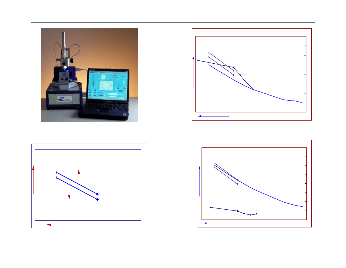
This technology predicts dynamic barite sag potential

through direct measurement of ultra-low shear rate
viscosity using a field viscometer (Figures 9 & 10).
Viscosity levels below the Lower Limit of the Prevention
Window correlate with severe dynamic barite sag
observed in the field and laboratory tests, and
correspond to a high potential for dynamic barite sag.

6

Conversely, viscosity levels above the Upper Limit
indicate a low potential for dynamic barite sag, but are
excessive in terms of requirements for barite sag
prevention. Finally, viscosity levels within the limits of
the Window are preferred, and indicate a low potential
for dynamic barite sag (Figure10). In terms of balancing
barite sag and ECD management, the viscosity profile of
the drilling fluid is optimized within the Window. Data
demonstrating correlation between this predictive
technology and the flow loop appears in Figures 11-12.

Drilling Variables Effecting Barite Sag
It was recently proposed that barite sag is not entirely a
mud-related problem, and that certain conditions in the
drilling operation are conducive to creating dynamic sag.
Bern et al.

8

presented a very comprehensive analysis of

these important variables and provided
recommendations in key areas involving well planning
and operational practices.

Several important findings

from this study were later verified by Dye et al.

6

In

particular, both studies identified a critical nominal

4

W. DYE, G. MULLEN

AADE–02-DFWM-HO-12

annular velocity value of 100 feet/minute, above which
barite bed formation is minimized in flow loop tests. In
the case of Bern et al., the value was identified in both
concentric and eccentric annuli and in combination with
pipe rotation. Dye et al. simulated an eccentric annulus,
but without pipe rotation.

Low shear rate conditions
The overall potential for dynamic sag is highest when the
drilling fluid experiences low shear rates. Flow loop data
and field observations suggest that severe dynamic sag
(> 1 lbm/gal) occurs under the combined influence of
insufficient viscosity levels (mud variable) and low
annular velocity (drilling variable). Sources of low shear
rate conditions include, but are not limited to, slow pump
rates, tripping pipe and wireline and pipe–conveyed logs.
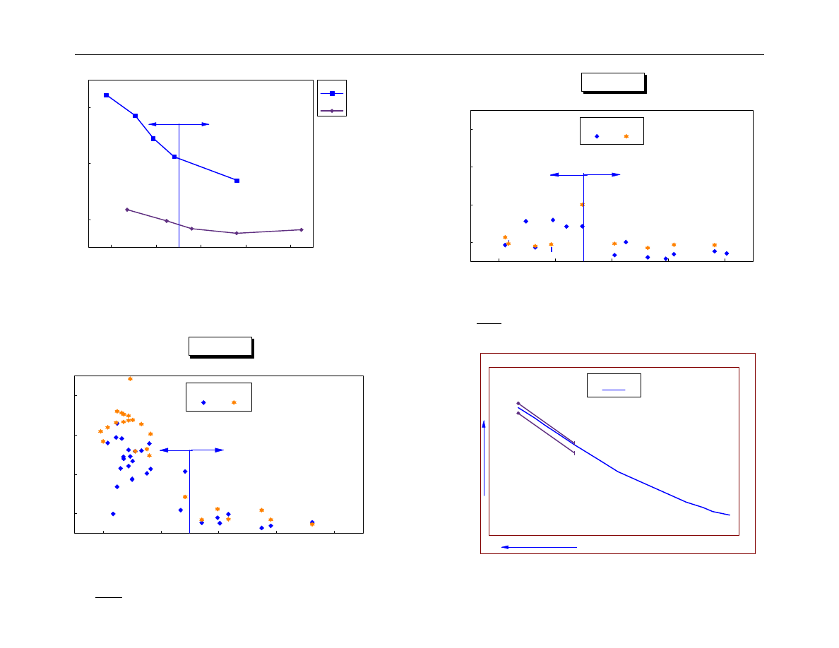
Figure 13 shows a comparison of dynamic sag and
average annular velocity for Muds #1 and #2. Dynamic
sag increased with both muds at nominal annular
velocity less than 100 feet/minute, although there were
differences in the severity of dynamic sag within this
region. Mud #1 represents a worst-case scenario in
terms of mud and drilling variables influencing dynamic
sag. The combined effect of insufficient viscosity (mud
variable) and low annular velocity (drilling variable)
resulted in dynamic sag levels as high as 2.73 lbm/gal
(Figure 11 & 13). On the other hand, Mud #2 exhibits
sufficient viscosity at ultra-low shear rates, which tends
to minimize, but not eliminate, dynamic sag arising from
low AV (Figure 12 & 13).

Figure 14 is a plot of flow data comparing dynamic

sag and nominal AV on fluids having viscosity levels
below the Lower Limit, and thus a high potential for mud-
related dynamic sag. The left-hand side of Figure 14,
where annular velocity is below 100 feet/minute,
corresponds to the highest levels of dynamic sag
measured in flow loop tests. Figure 15 shows a similar
comparison, however, this plot contains only those fluids
exhibiting a viscosity profile within the Window. The
main difference between Figures 14 and 15 is the
influence of drilling fluid viscosity on severe dynamic sag
at low annular velocity, or low shear rates.

Table 2 presents the overall dynamic sag potential

based on contributions from the mud and drilling
variables. The primary drilling variable presented in
Table 2 is nominal annular velocity because it is readily
available on the daily mud report. However, other
drilling variables, such as hole angle and pipe rotation
also effect dynamic sag. Low annular velocity can also
arise when tripping pipe or running casing, and may be
calculated using equation (2).

10

CF is the “clinging

factor” constant, which describes the ratio of pipe
diameter to hole diameter. Typical values of CF range
from 0.39 to 0.47.

(

)

Speed

Trip

PipeOD

HoleID

PipeOD

CF

AV

*

²

²

²















−

+

=

(2)

The influence of hole angle on dynamic sag is

enhanced at low annular velocity and with insufficient
drilling fluid viscosity. This trend is shown in Figure 14
when comparing the magnitude of dynamic sag at 60

°

and 45

°

at nominal annular velocity less than 100

feet/minute. In general, the highest level of dynamic
sag in flow loop tests occurred at the highest angle (60

°

).

The influence of angle on dynamic sag decreases with
proper control of ultra-low shear rate viscosity (Figure
15).

The following case history provides an example of

dynamic sag arising from influences of the drilling
operation.

Case History #4
A window was milled inside 11 7/8” casing and a
sidetrack section was drilled from 6,951 to 17,190 feet
using a 12 ¼” bi-center bit. Maximum angle in the
sidetrack section was 65°. The only problems
encountered in this section were associated with a
“ballooning” formation. Efforts to control the problem
required the operator to circulate at AV’s as low as 27
feet/minute in the open hole section.

Attempts to run a 9 5/8” liner stopped when the liner

became differentially stuck at 11,995’ feet, where it was
cemented into place, leaving 5,195 feet of 12 ¼” open
hole below the liner. A clean-out trip was made after
testing BOP’s and the well began ballooning, requiring
the operator to circulate at AV’s from 80 – 96 feet/minute
over the course of several days. Pipe was washed to
bottom at 19,946 and barite sag was observed when
circulating bottoms-up. Mud weights measured at the
shaker ranged from 12.5 to 14.7 lbm/gal, compared to a
nominal mud weight of 13.7 lbm/gal. This degree of
change in mud weight was unexpected since the
viscosity profile of the fluid was within the Window
(Figure 16), indicating a low potential for dynamic sag.
The expectation of those involved in the drilling
operation was that little, if any, change in mud weight
should occur since the viscosity curve was within the
Window.

Upon further review of the drilling variables involved,

it was apparent that the hydraulics of the circulating
system were compromised due to ECD management
concerns and ballooning. The annular velocity in the

≈

5200 feet of unplanned 12 ¼” open hole was
consistently below 100 feet/minute. The data presented
in Figure 15 suggests that the origin of dynamic sag was
low annular velocity (drilling variable), where moderate
levels (~ 0.5 – 0.8 lbm/gal) of dynamic sag arise when

AADE–02-DFWM-HO-12

New Technology to Manage Barite Sag

5

operating at low annular velocity.

Another potential source for fluctuations in mud

weights, particularly with invert-emulsion muds, is flow
line temperature. Unfortunately, the mud weight was
not reported in the context of a flow-line temperature on
this well. The density of invert-emulsion muds can
easily vary

±

0.3 lbm/gal with changes in flow-line

temperature; therefore, some portion of the variance is
attributed to temperature effects on base fluid density.

Conclusions

•

Shear rates experienced in eccentric annuli can
be significantly lower than in the concentric case,
and below the 3-rpm equivalent of the 6-speed
viscometer.

•

Trends observed in flow loop tests correlate with
field observations of dynamic sag.

•

Dynamic sag, defined as a mud weight variation,
occurred in all fluids tested in the flow loop. One
can determine acceptable levels of dynamic sag
in flow loop tests by comparing field and
laboratory results.

•

The RVT has two distinct sources of fluid
volumes; each sheared at different rates that
contribute to the mud weight change observed in
the test.

•

The RVT does not consider effects of pipe
eccentricity, annular velocity or hole angle on
dynamic sag and did not correlate with flow loop
results.

•

The Prevention Window accurately predicted
dynamic sag potential in all fluids evaluated on
the flow loop.

•

Dynamic sag arises from influences of the mud
system and the drilling operation, and these two
are often inter-related.

•

The potential for dynamic sag is enhanced when
operating at nominal annular velocity less than
100 feet/minute.

Acknowledgements

The Authors would like to express their appreciation

to

INTEQ Drilling Fluids for permission to release this

paper. We would also like to acknowledge the
contributions of Mike Vincent, Pat Kenny, Steve Spence
and Roland May to this paper.

Nomenclature

ECD = Equivalent circulating density

LCM = Lost circulation material

∆MW = Change in mud weight, lb

m

/gal

Rpm = Revolutions per minute

RVT = Rotational Viscometer Test

•

γ

= Shear rate, s

-1

or reciprocal seconds

D

o

= Diameter of outer cylinder

D

I

= Diameter of inner cylinder

F = Temperature,

°Fahrenheit

PV = Plastic Viscosity, cP

YP = API Yield Point, lb

f

/100 ft²

10 s Gel = API 10 second gel strength, lb

f

/100 ft²

10 m Gel = API 10 minute gel strength, lb

f

/100 ft²

θ3 = Fann viscometer readings at 3 rpm lb

f

/100 ft²

θ6 = Fann viscometer readings at 6 rpm lb

f

/100 ft²

LSRYP = (2 x

θ3) – θ6, lb

f

/100 ft²

AV = Average annular velocity, feet per minute

OD = Pipe outside diameter

ID = Piper internal diameter

CF = Clinging Factor

References

1.

Jamison, D.E., and Clements, W. R.:" A New Test Method
To Characterize Setting/Sag Tendencies of Drilling Fluids
In Extended Reach Drilling", ASME 1990 Drilling Tech.
Symposium, PD Vol. 27, pp. 109-113.

2.

Kenny, P. and Hemphill, T.: "Hole-Cleaning Capabilities of
an Ester-Based Drilling Fluid System", SPE Drlg & Comp.
March 1996.

3.

Saasen, A., Liu, D., and Marken, C.D.: " Prediction of
Barite Sag Potential of Drilling Fluids From Rheological
Measurements", SPE/IADC 29410, SPE/IADC
Conference, Amsterdam, Feb. 28 - March 2, 1995.

4.

Hanson, P.M., Trigg, T.K., Rachal, G. and Zamora, M.,
Sept 23-26, 1990, “Investigation of Barite “Sag” in
Weighted Drilling Fluids in Highly Deviated Wells”, SPE
20423, 65

th

Annual Technical Conference and Exhibition,

New Orleans, Louisiana.

5.

Bern, P.A., van Oort, E., Neusstadt, B., Ebeltoft, H.,
Zurdo, C., Zamora, M. and Slater, K., Sept 7-9, 1998,
“Barite Sag: Measurement, Modelling and Management”,
SPE/IADC 47784, Asia Pacific Drilling Conference,
Jakarta, Indonesia.

6.

Dye, W., Hemphill, T., Gusler, W., and Mullen, G., March
2001, “Correlation of Ultra-Low Shear Rate Viscosity and
Dynamic Barite Sag”, SPE 70128, SPE Drilling &
Completion.

7.

Dye, W., Mullen, G. and Ewen, B., “Recent Advances in
Barite Sag Technology”, presented at the American
Society of Mechanical Engineers ETCE 2002 Conference,
Houston, Texas 4-5 February 2002.

8.

Bern, P.A., Zamora, M., Slater, K.S., Hearn, P.J., October
6-9, 1996, “The Influence of Drilling Variables on Barite
Sag”, SPE 36670, SPE Annual Technical Conference,
Denver, Colorado.

9.

Jefferson, D.T., 1991, “New Procedure Helps Monitor Sag
in the Field”, 1991 Energy Sources Technology
Conference, New Orleans, Louisiana.

10. Burkhardt, J. A., “Wellbore Pressure Surges Produced by

Pipe Movement”, JPT, June 1961.

6

W. DYE, G. MULLEN

AADE–02-DFWM-HO-12

Table 1

Drilling Fluid Parameters

Sample Number

1

2

3

MW, @ 63

°

F

13.5 13.9 14.2

600 rpm

126

178

156

300 rpm

73

109

93

6 rpm

7

11

12

3 rpm

6

9

10

PV @ 120

°

F

53

69

63

YP @ 120

°

F

20

40

30

10 s Gel @ 120

°

F

9

13

13

10 m Gel @ 120

°

F

18

36

34

LSRYP, lb

f

/100 ft²

5

7

8

Average

∆

MW, lbm/gal (Flow Loop)

1.97 0.41 0.58

∆

MW, lbm/gal (RVT @ 100 rpm)

0.76 0.49

0.93

Table 2

Drilling & Mud Variables Affecting Dynamic Sag

Prevention Window

(MudVariable)

Nominal AV

(Drilling Variable)

Overall Dynamic Sag Potential

High Potential

< 100 feet/minute

High (Left-hand side of Figure 14)

High Potential

> 100 feet/minute

Low (Right-hand side of Figure 14 )

Low Potential

< 100 feet/minute

Low to moderate (Left-hand side of Figure 15)

Low Potential

> 100 feet/minute

Low (Right-hand side of Figure 15)

Appendix

–

Flow loop test procedures

Testing Preparation
1. Add ~ 20 gallons of drilling fluid to reservoir
2. Adjust test section to the desired angle
3. Adjust drill-pipe to the desired effective eccentricity
4. Heat to 120° F and circulate at maximum flow rate

Dynamic Barite Sag Testing
1. Confirm that density is uniform in test section
2. Reduce and maintain a constant pump rate for 30

minutes

3. Measure density at bottom and top sampling ports
4. Average density from bottom and top sections
5. Determine differential between bottom and top

sections

6. Flush test section by circulating at maximum flow

rate

Static Barite Sag Testing
1. Confirm that density is uniform in test section

2. Reduce flow rate to zero
3. Remain static for 16 hours at 120° F and desired

angle

4. Determine density differential as above

Flow loop Specifications

Test Section
1. 2-in ID x 6.7-ft length hollow metal pipe
2. 1-in OD stainless steel, fixed shaft
3. 5 evenly spaced sample ports on lower side
4. 4 evenly spaced sample ports on upper side
5. Wrapped insulation
6. Trace heating elements (± 1° F control)

Test Parameters
1. Flow rate: 0 – 40 gallons per minute
2. Average Annular Velocity: 0 – 288 feet per minute
3. Mud Volume: 15 - 20 gallons
4. Angle: 25° to 70°
5. Eccentricity: 0 – 100 %

AADE–02-DFWM-HO-12

New Technology to Manage Barite Sag

7

Figure 1. Barite Sag Flow Loop

Figure 2. Calculated annular shear rates in 12 ¼” hole

Figure 3. Case History #1 flow loop test results

Figure 4. Case History #2 flow loop test results

21" Riser/5" DP

12.4 " Casing/ 5" DP

12.25" OH/5" DP

12.25" OH/ 6 5/8" DP

12.25" OH/ 8" DC

10

20

30

40

50

2.5

17

18

28

45

2.5

0.4

0.45

1.28

3.4

Wellbore Components

Shear Rate, 1/s

Concentric

50 % Eccentric

0.05

0.1

0.2

0.5

1

2

5

10

2

4

Shear Rate, 1/s

Dynamic Sag, lbm/gal

Initial

Treated

2.4 lbm/gal difference in MW in field

0.5 lbm/gal difference in MW in field

0.1

0.3

1

3

10

1

2

3

Shear Rate, 1/s

Dynamic Sag, lbm/gal

Case History #2

0.8 lbm/gal difference in MW in field

8

W. DYE, G. MULLEN

AADE–02-DFWM-HO-12

Figure 5. Case History #3 flow loop test results

Figure 6. Geometry of RVT dynamic test

Figure 7. Technology comparison – flow loop results

Figure 8. Technology comparison – RVT results

0.1

0.3

1

3

10

1

2

3

Shear Rate, 1/s

Dynamic Sag, lbm/gal

Case History #3

0.75 lbm/gal difference in MW in field

0.1

0.3

1

3

10

0

1

2

3

Shear Rate, 1/s

Dynamic Sag, lbm/gal

Mud #1

Mud #2

Mud #3

0

10

20

30

10

11

12

13

14

15

16

Time, minutes

Density, lbm/gal

Mud #1

Mud #2

Mud #3

AADE–02-DFWM-HO-12

New Technology to Manage Barite Sag

9

Figure 9. RJF VISCOMETER





Figure 10. Prevention Window

Figure 11. Predictive technology & flow loop results–

Mud #1

Figure 12. Predictive technology & flow loop results–

Mud #2

Shear Rate, 1/s

Viscosity, cP

Low Potential for

Dynamic Sag

Low Potential for

Dynamic Sag

Upper Limit

Lower Limit

0

High Potential for

Dynamic Sag

0

1

2

3

4

Shear Rate, 1/s

Viscosity, cP

Dynamic Sag, lbm/gal

0

Viscosity

Dynamic Sag

Upper Limit

Lower Limit

0

1

2

3

4

Shear Rate, 1/s

Viscosity, cP

Dynamic Sag, lbm/gal

0

Viscosity

Dynamic Sag

Upper Limit

Lower Limit

10

W. DYE, G. MULLEN

AADE–02-DFWM-HO-12

Figure 13. Comparison of AV and dynamic sag in flow loop

tests on Muds #1 & #2

Figure 14. Annular Velocity vs. Dynamic Sag:

High Potential for Dynamic Sag from Mud Variable

Figure 15. Annular Velocity vs. Dynamic Sag:

Low Potential for Dynamic Sag from Mud Variable

Figure 16. Field viscometer measurements – Case

History #4

0

50

100

150

200

250

0

1

2

3

Average Annular Velocity, ft/min

Dynamic Sag, lbm/gal

# 1

# 2

100 ft/min

Below Window

Within Window

Below Window

0

50

100

150

200

250

0

1

2

3

4

Average Annular Velocity, ft/min

Dynamic Sag, lbm/gal

45°

60°

100 ft/min

Within Window

0

50

100

150

200

250

0

1

2

3

4

Average Annular Velocity, ft/min

Dynamic Sag, lbm/gal

45°

60°

100 ft/min

Shear Rate, 1/s

Viscosity, cP

Case History #4

0

Upper Limit

Lower Limit