8290614307

7. Opublikowane badania własne

7. Opublikowane badania własne

91

J. Orzeł et ol: Oirmomrincs and InrrUttent Loborotory Sytiem 110 (2012) 99-96

(11)

Initialization of leverage and residual weights is an important step that has an cffcct on method convergence. initial estimates of leverage weights can be found according ro Eq. (7) by replacing the PRM scores with expianatory variables and Eq. (8). Initial residua) weights can be estimated using Eq. (9). where residuals are substituted by centered elements of the response variabłe around median and then Eq. (8).

The PRM method is one example of a robust variant of the classic PLS-1 method. Morę robust calibration techniques are presented and discussed in |20-23|. Compared to other robust variants of PIS. PRM has a high computational speed and withstands a relattvely large number of outliers 119J.

22.1. Identification of ouiliers/srudymg outlying character of objects Once the PRM model is construaed and using its parameters. it is possible to identify outlying objects in a calibration set (and test set, if deemed necessary) and/or ro find out reason for their oudyingness. For objects from the calibration set. their robust standardized dis-tances in the model space of/PRM latent factors. d‘ and standardized residuals. d; are evaluated:

!it,-Llmed(T)||

‘*Q_nn:t_ł-Llmed(T)||)

the outlying character of an object in the model space and/or with respect to the model fit (residuals).

In relation to objects from test set. it is also possible to find out the reason for their outlyingness by evaluating the respective residuals and PRM scores. For this purpose, test set objects are projected into the PRM model space in order to obtain their scores and then robust distances (assuming weights for the test samples equal to one). How-ever. it should be emphasized that diagnostics of outlying objects in a test set using the distance-distance plot can provide some insight only at the stage of robust model construction, Le. response values are available for objeas from test set (e^, after splitting the availabie data into model and test sers).

The finał PRM model is constructed when the algonthm'$ conver-gence is achieved. Then. the weights for all objects are esublished and influence of outlying objects on the model is reduced. Although the finał PRM model is optimal it is also possible to dlscard outliers using the distance-distance plot to consrmct the finał model using the classic PIS approach. This step can be regarded as fine runing the finał calibration model sińce with the classic PLS model morę efficient estimates of the regression coefficient are derived as compared to PRM.

2.4. Selection of the model set

_<=ir_lZmedm₁

r)

where <r_Qn is the robust Qn estimator of the data scalę 119).

For both distances. d? and d[. the cutoff values are defined by assuming normal distribution of data majority. The cutoff values divide the model space into four regions containing different types of objects. They can be visualized in a so-called distance-distance plot. presented in Fig. 1. where the standardized residual distances of objects are pkmed versus their standardized leverage distances. With respect to df and d\ one can distinguish among three types of outlying objeas: bad leverage objects (with long teverage distances. Le. locat-ed far away in the PRM model space from data center and with long residual distances). high residual objects (with long residual distances and shorr leverage distances) and good >everage objects (with long leverage distances but short residual distances). By setting the cutoff value to 3. it is expeaed that 99.9% of objeas will have d1 and d'_t distances shorter than the cutoff value.

In order ro rapidly grasp why objects from the model set are outlying. one can inspea leverage and residual weights of the PRM model simultaneously (using a plot similar to the distance-distance plot). Depending on the weight type. a large magnirude indicates

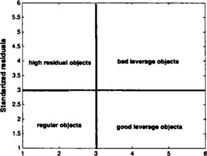
Standarlzed dicUnc** In ■paca of PRM model Fig. 1. Lumpie of » diłuner disuncr płoł for robtitt panul Iran squires modcl

Construaion of any calibration starts with the seieaion of model and test sets. Objects in the model set are used for construction of the model and samples from the test set for validation of the model. Construaion of a reliable calibration model - with good prediaion properties - requires uniform sampłing of the expcrimental domain as well as including all of the sources of dau variation into the model set [24|. There are several efhdent uniform subset selection algorithms well suited for this purpose |24|. Among the most popular on es are the Kennard and Stone (KAS) and the Duplex algorithms (25.261. In both algorithms. samples are selrcted into a model set on the basis of the maximal dissimilarity among samples scored using the Euclidean distance. In the context of calibration. the main advan-tage of the Duplex algorithm over KAS is that the model and test sets are represenutive (ie. samples in the model and test sets are uni-formly scattered over the experimental domain).

2.5. Seieaion of model complexity and sconng its prediction ability

One of the most important steps during the construaion of the calibration model is the choice of the optimal number of latent iac-tors, fi which is frequendy supported by using the CTt>ss-validation procedurę (CV) (27|. During cross-validation. a subset of p objects is removed from the dau and these objeas form the test seL A calibration model is aeated for the remaining objects and the root mean square error of cross-validation. RMSECV. is calculated for the test set objects. The procedurę is repeated and the next subset of objects is removed from the dau for which a number of models with an inereasing number of latent factors are constTucted. This is done unril all possibilities for the construaion of the subsers are exhausted. For each latent faaor. the corresponding RMSECV is reported as an average value and calculated as:

RMSECV(/| = !    (y.-y.)¹    (13)

\”t*l

where. y, is the experimenul value of the response variable and y, is the prediaed value of the response variable.

There are different variants of the cross-validation procedurę. e.g. the leave-one-out cross-validation (LOOCV). the leave-more-out cross-validation (LMOCV) and the Monte Carlo cross-validation (MCCV). LOOCV is the most popular approach; however. LMOCV or MCCV are recommended sińce they provide morę accurate estimates

Strona 54