ISSN 0105-3027
An Auditory Model with
Hearing Loss
THE ACOUSTICS
LABORATORY
TECHNICAL UNIVERSITY OF DENMARK
Report No.
52,
1993

An Auditory Model with Hearing Loss.
Lars Bramsløw Nielsen
Oticon Research Unit "Eriksholm"
and
The Acoustics Laboratory
Technical University of Denmark

Page 2
An auditory model with hearing loss.

An auditory model based on the psychophysics of hearing has been developed and tested.
The model simulates the normal ear or an impaired ear with a given hearing loss. Based
on reviews of the current literature, the frequency selectivity and loudness growth as
functions of threshold and stimulus level have been found and implemented in the model.
The auditory model was verified against selected results from the literature, and it was
confirmed that the normal spread of masking and loudness growth could be simulated in
the model. The effects of hearing loss on these parameters was also in qualitative
agreement with recent findings. The temporal properties of the ear have currently not
been included in the model.
As an example of a real-world application of the model, loudness spectrograms for a
speech utterance were presented. By introducing hearing loss, the speech sounds
became less audible and less detailed, a problem that linear amplification did not solve
properly. This demonstrated how the model could be used for hearing aid development
and evaluation.
Abstract.
An auditory model with hearing loss.
Page 3
Abstract

Page 4
An auditory model with hearing loss.
Abstract

This report describes the development and structure of an auditory model for objective
evaluation of sound quality in hearing aids. Since the model is intended to model a
hearing-impaired listener, the hearing loss has been included as a parameter in the model,
affecting sensitivity as well as frequency resolution and loudness perception. Such a
model should attempt to unite all known aspects of psychoacoustics for normal-hearing
and hearing-impaired listeners into a coherent picture, which is obviously an impossible
goal. The current model is a result of many compromises and represents a first,
simplistic attempt at such a unification.
The report deals with many psychoacoustic terms in a limited amount, and is thus on a
fairly advanced level. The reader is expected to be familiar with basic psychoacoustics,
to read the report with a good understanding. Good introductory texts can be found in
Zwicker & Fastl (1990), Scharf & Buus (1986) and Scharf & Houtsma (1986).
The model is just one of the elements covered in the entire Ph.D. project "Modeling of
sound quality for hearing-impaired listeners", and limited time has thus been available for
exploration of a large and complex topic. The Ph.D. project is a joint project between
Oticon A/S and The Acoustics Laboratory, Technical University of Denmark, and the
report has thus been published by both parties: Oticon Internal Report No. 43-8-2 and
The Acoustics Laboratory, Technical report no. 52.
Preface.
An auditory model with hearing loss.
Page 5
Preface

I want to acknowledge my advisors for their support and valuable discussion during the
work with this model: Claus Elberling, Oticon A/S, Torben Poulsen, The Acoustics
Laboratory and Paul Dalsgaard, Center for Speech Technology, Aalborg University
Center. Furthermore, I want to express my gratitude to Søren Buus and Mary
Florentine, Northeastern University, Boston, for many critical and useful suggestions
during the last phase of evaluations and modifications of the model.
Lars Bramsløw Nielsen
Snekkersten, February 1993
Page 6
An auditory model with hearing loss.
Preface

73
6. Conclusion.
. . . . . . . . . . . . . . . . . . . . . . . . . . . . . . . . . . . . . . . . . . . . . . . . . . .
71
5.2 Performance and future improvements.
. . . . . . . . . . . . . . . . . . . . . . . . .
69
5.1 Perception of speech sounds. . . . . . . . . . . . . . . . . . . . . . . . . . . . . . . . . . .
69
5. Processing of real-world signals. . . . . . . . . . . . . . . . . . . . . . . . . . . . . . . . . .
68
4.4 Temporal resolution.
. . . . . . . . . . . . . . . . . . . . . . . . . . . . . . . . . . . . . . . .
67
4.3.2. Equal loudness level contours. . . . . . . . . . . . . . . . . . . . . . . . . . . .
61
4.3.1. Loudness growth in normal and impaired hearing.
. . . . . . . . . . .
61
4.3 Loudness. . . . . . . . . . . . . . . . . . . . . . . . . . . . . . . . . . . . . . . . . . . . . . . . . .
58
4.2.3. Impaired frequency selectivity. . . . . . . . . . . . . . . . . . . . . . . . . . . .
56
4.2.2. Noise signals. . . . . . . . . . . . . . . . . . . . . . . . . . . . . . . . . . . . . . . . . .
53
4.2.1. Excitation patterns, pure tones. . . . . . . . . . . . . . . . . . . . . . . . . . . .
53
4.2 Frequency selectivity. . . . . . . . . . . . . . . . . . . . . . . . . . . . . . . . . . . . . . . . .
53
4.1 Test design and stimuli. . . . . . . . . . . . . . . . . . . . . . . . . . . . . . . . . . . . . . .
53
4. Verification. . . . . . . . . . . . . . . . . . . . . . . . . . . . . . . . . . . . . . . . . . . . . . . . . . . .
52
3.6 Temporal processing. . . . . . . . . . . . . . . . . . . . . . . . . . . . . . . . . . . . . . . .
51
3.5.2. Loudness summation in hearing-impaired listeners. . . . . . . . . . . .
46
3.5.1. As a function of level and threshold. . . . . . . . . . . . . . . . . . . . . . . .
46
3.5 Loudness function. . . . . . . . . . . . . . . . . . . . . . . . . . . . . . . . . . . . . . . . . . .
41
3.4.3. Filter shape as a function of level and hearing loss. . . . . . . . . . . .
36
3.4.2. Filter shape as a function of hearing loss. . . . . . . . . . . . . . . . . . . .
33
3.4.1. Filter shape as a function of level. . . . . . . . . . . . . . . . . . . . . . . . . .
28
3.4 Auditory filter bank. . . . . . . . . . . . . . . . . . . . . . . . . . . . . . . . . . . . . . . . . .
23
3.3 Equalizations and coupler corrections. . . . . . . . . . . . . . . . . . . . . . . . . . .
22
3.2 Power spectrum calculation. . . . . . . . . . . . . . . . . . . . . . . . . . . . . . . . . . .
20
3.1 Model structure. . . . . . . . . . . . . . . . . . . . . . . . . . . . . . . . . . . . . . . . . . . . .
20
3. Model description. . . . . . . . . . . . . . . . . . . . . . . . . . . . . . . . . . . . . . . . . . . . . .
18
2.5 Psychophysical measurements. . . . . . . . . . . . . . . . . . . . . . . . . . . . . . . . .
17
2.4 Auditory models. . . . . . . . . . . . . . . . . . . . . . . . . . . . . . . . . . . . . . . . . . . .
16
2.3 Cochlear modeling problems. . . . . . . . . . . . . . . . . . . . . . . . . . . . . . . . . .
13
2.2 Physiological measurements. . . . . . . . . . . . . . . . . . . . . . . . . . . . . . . . . . .
11
2.1 Cochlear models. . . . . . . . . . . . . . . . . . . . . . . . . . . . . . . . . . . . . . . . . . . .
11
2. Literature review. . . . . . . . . . . . . . . . . . . . . . . . . . . . . . . . . . . . . . . . . . . . . . .
9
1. Introduction. . . . . . . . . . . . . . . . . . . . . . . . . . . . . . . . . . . . . . . . . . . . . . . . . . . .
Table of contents.
An auditory model with hearing loss.
Page 7
Table of contents

90
8.2 Proposed UCL-encoding.
. . . . . . . . . . . . . . . . . . . . . . . . . . . . . . . . . . . .
87
8.1.2. Command-line usage. . . . . . . . . . . . . . . . . . . . . . . . . . . . . . . . . . . .
82
8.1.1. Input parameter file format. . . . . . . . . . . . . . . . . . . . . . . . . . . . . . .
81
8.1 User manual. . . . . . . . . . . . . . . . . . . . . . . . . . . . . . . . . . . . . . . . . . . . . . . .
81
8. Appendices. . . . . . . . . . . . . . . . . . . . . . . . . . . . . . . . . . . . . . . . . . . . . . . . . . . .
75
7. References. . . . . . . . . . . . . . . . . . . . . . . . . . . . . . . . . . . . . . . . . . . . . . . . . . . . .
Page 8
An auditory model with hearing loss.
Table of contents

The human auditory system is a very sophisticated and complicated signal processing
system that is capable of perceiving and analyzing very complex sounds and
discriminating subtle changes in sound. These characteristics are crucial for the
perception and recognition of speech and for interpretation of the sound patterns
encountered in daily life, as well as for enjoyment of music. The normal hearing system
can be damaged due to aging, otologic diseases, exposure to loud noises, ototoxic drugs
and other reasons. This will often result in a communication handicap, due to loss of
sensitivity and impaired discrimination of speech sounds as well as other auditory stimuli.
Much research has been done to further our understanding of the human hearing system,
but there is still very limited knowledge concerning the function of the system on a
physiological level as well as on a psychological level, i.e. in the disciplines auditory
physiology and psychoacoustics. Research results are often summarized in mathematical
or verbal models, to explain a certain phenomenon in a meaningful way and to allow the
application of the model to other similar problems. Models of psychoacoustic
phenomena, such as frequency masking, have provided much insight into the function of
the hearing system (Zwicker & Fastl, 1990).
When modeling functional parts of the hearing system and applying these models to for
instance speech sounds, we often refer to them as cochlear models or auditory models.
In the literature, these terms are sometimes used interchangeably. In this report, the term
cochlear model refers to a model that takes its origin in the physiological macro- and
micro-mechanics and neural function of the cochlea. An auditory model describes the
auditory function on a higher "black-box" level and attempts to model psychoacoustical
phenomena correctly, with little or no attention concerning a possible anatomic location,
e.g. whether the characteristics are peripheral (frequency selectivity, active tuning) or
more central (probably aspects of loudness and temporal resolution). Some of the
auditory models in the literature are mixed, including results from both physiology and
psychoacoustics.
1
Introduction.
An auditory model with hearing loss.
Page 9
1. Introduction

An introduction to two of the published cochlear models and two auditory models has
been given by Fink (1989), these are summarized in section 2 of the present report.
None of these models include the case of impaired hearing, i.e. hearing loss. The present
report describes the development and evaluation of such a model:
In section 2, literature review, a number of existing models are presented. The issues
concerning cochlear (physiological) versus auditory (psychoacoustical) models are
discussed. After reviewing literature on auditory models and psychoacoustical
measurements, the choice of an auditory model is justified.
Section 3 is a detailed description of the model and the underlying theories and
psychoacoustical test paradigms. The elements in the model are discussed: Frequency
selectivity, temporal resolution, loudness coding and hearing loss. Suitable tests for
verification of the model are also discussed.
In section 4 verification results for the model are presented. The purpose is to duplicate
known psychoacoustic test results from the literature, by means of the model and thereby
justifying that the model simulates average cases of normal and impaired hearing.
In section 5 one application of the model is demonstrated: Analysis of normal and
amplified (frequency shaped) speech signals for the normal-hearing case and for a typical
sensorineural, sloping hearing loss.
Page 10
An auditory model with hearing loss.
1. Introduction

2.1
Cochlear models.
Several authors have presented models in the literature intended to mimic the
physiological function of the cochlea more or less. One motivation for this work was to
develop perceptually relevant pre-processors for automatic speech recognition systems.
Partly because of this, there has been little or no interest in models of the impaired
cochlea. More recently two authors have included hearing loss in their cochlear models
(Allen, 1990; Kates, 1991). Understanding the functionality of cochlear models requires
basic knowledge of the human auditory physiology, see for instance Pickles (1982).
Allen (1985) offers a good overview of cochlear modeling, including a summary of his
own work. Models are described for the outer ear (pinnae), middle ear and cochlea, with
an emphasis on the latter part. The mechanisms for the basilar membrane, Corti's organ,
and tectorial membrane are discussed. A fundamental problem in cochlear
micromechanics is the discrepancy between the basilar membrane mechanical tuning
curves and the much sharper neural tuning curves. Two explanations are offered for this
very sharp tuning exhibited by the normal cochlea. The first explanation assumes that
the tectorial membrane is resonant and tuned to a slightly different frequency, thereby
introducing additional zeros in the transfer function between basilar membrane motion
and hair cells. The second explanation (Neely and Kim, 1983) calls upon the concept of
negative damping in the basilar membrane, based on an active feedback system, in which
the outer hair cells are innervated by efferent nerve fibers and act as motor cells. There
is no clear evidence as to which explanation is more correct.
The output from the mechanical model is then fed to a hair-cell model, followed by
zero-crossing detector. By processing speech sounds through the model, the output of
this detector is used to form a "neurogram", i.e. a neural equivalent of a spectrogram,
which is an x-y-z time-frequency plot of a signal. This neurogram shows some ability to
enhance speech or pure tones in noise, as the human hearing system is capable of (typical
detection threshold of a pure tone in narrow-band noise is at negative signal-to-noise
2
Literature review.
An auditory model with hearing loss.
Page 11
2. Literature review

ratio). In a later paper (Allen, 1990), a model for the noise-damaged cochlea is
described. The reduced frequency selectivity can be accounted for by a reduced stiffness
of the basilar membrane. Allen offers the following hypothesis: In the normal cochlea,
the BM stiffness is increased due to the active-feedback process from the outer haircells,
that act as motor cells, rather than sensory cells. There is evidence that the outer
haircells are damaged by noise exposure, thus reducing or destroying the active system.
The model described by Seneff (1984, 1985) contains a 40-channel critical-band
filterbank, implemented as a cascade of zeroes (notch filters), followed by a resonator
between each cascade section, to form a 40-channel parallel output. This filter structure
simulates the basilar membrane and the traveling-wave motion along it, and sufficiently
sharp tuning curves are obtained. There is no active feedback process in the filter
structure. Each resonator output is then followed by two automatic gain Controls
(AGC) in order to effect amplitude compression and adaptation phenomena. The signal
is then fed to a saturating half-wave rectifier, acting as a hair-cell model. The outputs of
this "peripheral" model is subsequently processed by a hypothesized "central" processor -
an envelope/synchrony detector. This detector serves to detect prominent periodicities
in the input waveform, in order to estimate fundamental frequency and formant structure
for an incoming speech signal.
Lyon (1982) and Lyon & Dyer (1986) have developed a cochlear model consisting of
simple second-order notch filter sections in cascade. Resonance sections mimic the
tectorial membrane resonance, followed by detectors and a multi-channel AGC coupled
across channels (implementing a "spatial spread" function along the basilar membrane).
The model is characterized by a large number of simple processing elements and a high
degree of parallelism. An analog Very Large Scale Integrated (VLSI) chip
implementation is thus feasible and has been presented by Lyon and Mead (1988), with a
resolution of 480 channels.
Kates (1991) has developed a digital cochlear model, that allows for a degradation
related to hearing impairment. The model consists of the middle ear, the mechanical
motion of the basilar membrane and the neural transduction of the hair cells. The
Page 12
An auditory model with hearing loss.
2. Literature review

traveling waves on the cochlear partition are represented by a cascade of second-order
resonant lowpass filters. The displacement output is then differentiated to obtain the
velocity and fed through a second filter, that is hypothesized to result from the resonance
in the motion between the basilar membrane and the tectorial membrane. The second
filter is followed by a hair cell model, and each hair cell has four nerve fibers attached to
it, using both low- and high-spontaneous firing rate fibers. In Kates' cochlear model,
there is an active feedback path, that sharpens the filter selectivity at low signal levels,
suggested as a simulation of an active outer hair cell feedback mechanism. Hearing
impairment can be simulated by either removing the feedback (corresponding to
complete loss of outer hair cells) or by removing parts of the inner hair cells hairs
(stereocilia). With loss of outer hair cells, the filter system becomes linear with loss of
the normally improved frequency selectivity at low levels. With loss of inner hair cell
stereocilia, the overall sensitivity is reduced. This can be alleviated by amplification,
however the higher signal levels will then cause a broadening of the cochlear filters.
In my opinion, Kates' model is an important step towards using cochlear models for the
study of hearing impairment and potentially useful signal processing strategies, at least
on a qualitative level. It is not clear, however, how a given hearing loss (expressed by
the hearing thresholds in the audiogram) is simulated quantitatively. Specification of the
loss of outer and inner hair cells in the model due to hearing impairment is very difficult,
only rough estimates can be used. Another problem with this model as with other
cochlear models, is that they are computationally very intensive. Kates' model requires
1.5 s per sample on an 8 MHz IBM PC-AT, which at 40 kHz sample rate means 60.000
times real time.
2.2
Physiological measurements.
All the physiologically based (cochlear) models must be based on some type of
physiological measurements on humans or animals with similar auditory physiology (such
as the cat). In particular, we are interested in the frequency analyzer capabilities of the
cochlea, i.e. the frequency selectivity in the system. Making these physiological
measurements is very difficult, since the introduction of measurement probes or other
An auditory model with hearing loss.
Page 13
2. Literature review

objects in the very delicate system normally damages or at least interferes with the
normal cochlear function. Therefore, there are still many unanswered questions
concerning the mechanics and physiology of the cochlea. Measurements of the basilar
membrane movements and mechanical tuning have been done using mechanical or optical
techniques, requiring the intrusion into the cochlea for the placement of measurement
probes, mirrors or other objects onto the basilar membrane. This must be done on live
animals (in vivo), but the intrusion nevertheless ruptures membranes, disturbs the
cochlear fluids and thus the cochlear potentials etc., making valid results difficult to
obtain.
Another way of characterizing cochlear frequency selectivity is by means of
neurophysiological measurements. This is typically done by inserting very thin
measurement electrodes into single nerve fibers in the auditory nerve (8th nerve) that
connects the cochlea to the brainstem. The individual fibers in the nerve are
tonotopically arranged, i.e. a given fiber represents a given location along the basilar
membrane. The corresponding frequency is called the Characteristic Frequency (CF) of
the fiber. The frequency selectivity of a fiber, can be measured by adjusting the level of a
swept pure tone up and down to maintain a constant spike activity in the nerve. The
resulting curve is loosely referred to as "tuning curves", or more precisely, as Frequency
Threshold Curves (FTC). Since the FTC includes the mechanical tuning system as well
as hair-cell transduction and possible interaction between different regions in the cochlea,
it is likely that the micro-mechanics of the cochlea cannot be deduced from the neural
tuning data.
For further information on cochlear physiology and overview of measurement
techniques, see for example Pickles (1982).
The shape of FTCs recorded from single nerve fibers in the 8th nerve of a cat, using a
single pure tone, have been quantified by Evans (1975a). These curves show the dB
SPL of a swept sine wave required to produce a constant spike-rate in a nerve fiber, thus
they are iso-rate curves. The shape is described by the low-frequency slope (the slope of
the tail), the Q
10dB
(the 10dB Q of the tip, used instead of the usual 3 dB point due to the
Page 14
An auditory model with hearing loss.
2. Literature review

sharpness of the tip) and the high-frequency slope. By repeating the sweep for many
individual nervefibers tuned to different Characteristic Frequencies (CF), the three
variables can be plotted as function of frequency. It is common practice to transform the
CF of each nervefiber one octave down from cat to man, since the auditory bandwidth of
cat is 40 kHz, as opposed to 20 kHz in man. Consequently, the CF values for cat must
be halved to be interpreted as human CF values.
If the tuning curves are assumed to originate from a bank of linear filters, they can be
interpreted as the inverse of the filter frequency response. They should thus be the result
of a passive, mechanically tuned system and the shape should be independent of level. It
is hypothesized by some authors that the cochlea also provides an active mechanism with
negative feedback (Neely & Kim, 1983) or AGC (Lyon, 1982) to provide a sharper
tuning at the tip of the tuning curve. Adaptive-Q filter models have been proposed by
Hirahara and Komakine (1989) and by Kates (1991), these essentially model the same
properties. The resulting tuning curves are then level-dependent and we can speak of a
non-linear filterbank. This active function can be explained by active outer hair cells that
are innervated from the brainstem or elsewhere in the cochlea (via efferent nervefibers)
and act as motor cells to produce a displacement of the basilar membrane. Lyon's
AGC-model exhibits sharp tuning when tuning curves are determined by means of pure
tone sweeps, due to the AGC adapting as the stimulus frequency passes the tip of the
FTC.
An average fixed frequency response (the linear component) can be more accurately
determined by the reverse correlation (RevCor) method, where the impulse response of
individual nerve fibers is determined using lowpass filtered noise as the input. The
method has been used by Evans (1985) and many others. For a particular fiber, or CF,
the input signal is constant (or slowly fluctuating), and the presumed AGC is in a
stationary mode. If, however, the active section is a cochlear amplifier acting on the
instantaneous signal value, the results obtained from the RevCor method should in
principle be identical to those of the pure tone sweep.
An auditory model with hearing loss.
Page 15
2. Literature review

The above examples illustrate that there are different measurement techniques and
different theories to explain the tuning properties of the cochlea, and that there is not a
single, uniform theory for the cochlear frequency selectivity.
2.3
Cochlear modeling problems.
The neurophysiological measurements yield compound data, because many elements are
included between the two measurement points: tympanic membrane sound pressure and
single fiber activity. The chain includes mechanical tuning in the basilar and tectorial
membranes, transduction in the hair cell (mechanical-electrical conversion), active tuning
mechanisms (presumably due to active outer hair cells), nerve-interconnections in the
cochlea (lateral inhibition, if existing), and haircell-synapse-nervefiber connection.
Derivation of the various elements in the model, including data for the design of a
cochlear filterbank, becomes a very difficult task.
The neural data found in the literature, is highly variable when it comes to the shapes and
slopes of tuning curves. Moreover, the data is typically based on animal measurements.
The effects of hearing loss has been simulated by either causing a noise-induced loss
(Liberman and Dodds, 1984) or through the use of ototoxic drugs (Harrison and Evans,
1982). A normal age-induced loss cannot easily be controlled, which is probably the
reason that it was never evaluated. Modeling the normal and impaired ear, including
level-dependent filter characteristics, would thus be based on a weak foundation. More
consistent data are available from psychophysical measurements (see below). The same
conclusion was reached by Leijon (1989), who chose a psychoacoustical model to model
the impaired ear for the purpose of hearing aid evaluation. Leijon also emphasizes that
the computational complexity of a physiological model with high sample rates all the way
to the nerve-fibers would require many hours of computer time to process seconds of a
speech signal. This problem was also evident in another cochlear model (Kates, 1991).
If a model is based on tuning curves of single nervefibers, it should ideally feature a large
number of channels, perhaps on the order of 30000, similar to the number of nervefibers
in the auditory nerve. This number of channels is obviously un-realistic and should for
Page 16
An auditory model with hearing loss.
2. Literature review

practical purposes be limited to roughly 30-40 channels in the current study. In that
case, the single-fiber analogy has little meaning, and some kind of critical-band model
appears more appropriate.
2.4
Auditory models.
These models are primarily based on psychophysical measurements and are to some
extent "black-box" models, in the sense that they model simple psychophysical
properties, such as frequency masking, loudness growth etc. Certain aspects from the
auditory physiology can be included, for example models of the hair cell.
The model described by Cohen (1989) calculates the energy in 20 non-overlapping
critical bands (CB) from a 512-point FFT. The energy is then converted to loudness
level (phon) by means of a histogram method over 10 seconds of speech, where
estimates of threshold and uncomfortable levels are adjusted adaptively. Loudness (son)
is then calculated based on Stevens' power law. Temporal effects are added, using a
hair-cell model for short-term adaptation, similar to Seneff (1985).
Hermansky (1990) has proposed another model based on critical bands. The power
spectrum obtained from a windowed, 256-point FFT is warped onto a Bark critical band
scale and convolved by a critical-band curve given by a piece-wise linear approximation.
This excitation pattern is then sampled at app. 1-Bark intervals, obtaining 18 samples
(channels). To simulate an equal loudness curve, the critical band energy is
pre-emphasized by an approximated frequency response, derived from normal
equal-loudness contours. The last operation is a cubic-root amplitude compression, to
obtain loudness in each band (specific loudness). For speech analysis, an autoregressive
linear prediction analysis is performed on the loudness data from the auditory model.
The model has no dynamic or adaptive effects included and according to the author, the
choice of calculation models was often motivated by the need for computational
efficiency.
Karjalainen (1985, 1987) has implemented a 48-channel auditory model, using FIR
filters, instead of the common FFT-analysis. The power spectrum is obtained by
An auditory model with hearing loss.
Page 17
2. Literature review

squaring and lowpass-filtering by a fast linear filter. A non-linear filter is then applied to
simulate temporal integration and post masking. The output is converted to dB to the
end result, the "auditory spectrum". A small study on just-noticeable differences (JND)
of distortion indicates (Karjalainen, 1985), that it is correlated to the "auditory spectrum
distance", which is the maximum difference in dB between the auditory spectrums for the
unprocessed and the distorted signal. This is the only application of auditory models for
sound quality measurements that has been found in the literature.
Leijon (1989) has developed an auditory model with cochlear hearing loss. This model is
used for optimization of hearing-aid gain according to the proposed Loudness versus
Entropy Optimization (LEO) method. This algorithm attempts to increase the estimated
speech intelligibility, while keeping the total aided loudness at a pre-determined level.
The main characteristics of cochlear hearing impairments, such as rapid growth of
loudness, impaired auditory frequency resolution, and impaired auditory time resolution,
are explicitly included in the auditory model.
2.5
Psychophysical measurements.
For the design of a filter bank, auditory filter shapes derived from psychophysical
measurements must be modeled. The shape of these filters is not identical to the
narrow-band noise masking pattern, one type of excitation pattern often used to
characterize auditory filtering. However, the excitation pattern for a given stimulus can
be derived from the auditory filter shape - the excitation pattern will be the output from
an auditory filter bank as a function of filter center frequency.
The auditory filter shapes can be derived from thresholds of pure tones masked by
notched-noise with varying notch width (Moore and Glasberg, 1983). The auditory
filters here have Equivalent Rectangular Bandwidth (ERB) corresponding to 30 channels
for the range 0.1 - 8 kHz. Glasberg and Moore (1986) provide data on normal-hearing
and hearing-impaired listeners, according to a filter shape model (rounded exponential,
or roex) described by Patterson et al (1982). Additional data on filter shapes at low
frequencies for normal- and hearing-impaired listeners have been published by Peters and
Page 18
An auditory model with hearing loss.
2. Literature review

Moore (1992). This data is appropriate for modeling, since analytical expressions of
filter shapes are available for listeners with and without hearing loss, obtained in the
same experiment. The filter parameters found by Glasberg and Moore (1986) and by
Tyler et al (1984) are in some cases significantly correlated to hearing threshold,
however it is pointed out, that filter characteristics may vary considerably for identical
hearing losses due to individual and etiologic differences.
For the current auditory model, the question then arises, whether a representative
auditory model would require masking experiments on each subject to obtain accurate
estimates of filter parameters, or whether these can be derived from absolute thresholds.
The current model makes a generalization, by deriving these parameters from hearing
loss, which must necessarily be done if one wants to predict performance for a
population. The validity of this generalization should always be regarded with caution.
The model for derivation of excitation patterns (which would be the output of an
auditory filterbank) is based on the long-term power spectra of the stimulus, and
temporal fluctuations, as in all speech signals, are disregarded. For an auditory model,
meant for processing of real-world signals, the temporal behavior of the model is an issue
to be considered.
In order to model hearing loss, level-dependent frequency selectivity and loudness in a
single, coherent model, data from several studies must be combined. This also requires
combining data obtained under different experimental conditions, and perhaps even with
different conclusions.
An auditory model with hearing loss.
Page 19
2. Literature review
This section specifies the present model, which has been based on review of current
literature on auditory models and psychophysics. No experimental psychophysical work
was done for the development of the model. In its current state, the model represents a
mixture of information from various authors, since a complete model, including hearing
loss is needed. No single source has previously described such a model, except for
Leijon (1989), which was not known at the time the present model was developed.
There are many similarities between the two, however, Leijon has not examined the
psychophysical data on which his model is based, and there is no evaluation of the model
with respect to psychophysical results from the literature.
3.1
Model structure.
The emphasis in the current model is to describe the peripheral hearing function with
respect to perception of sound quality, as opposed to (for instance) speech recognition.
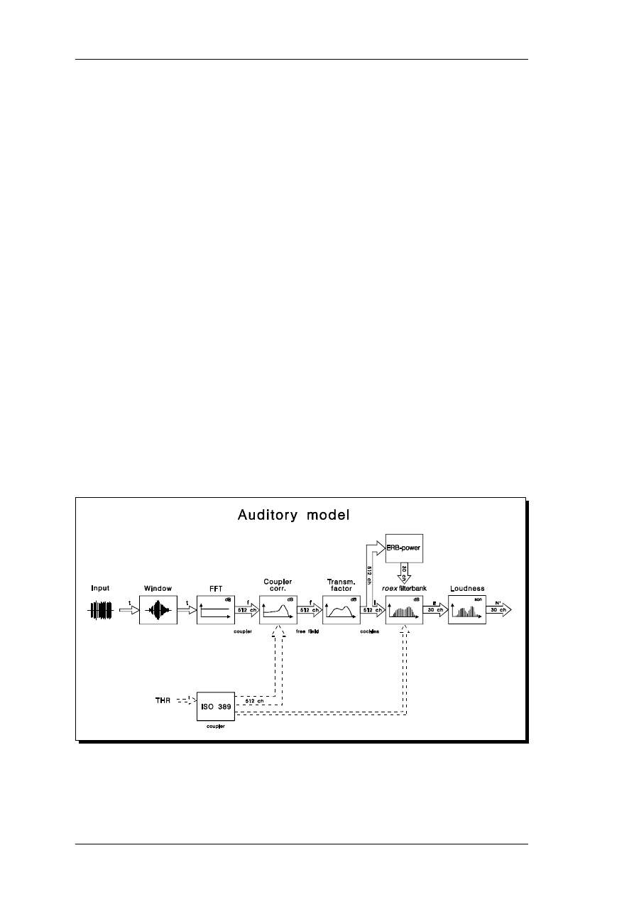
A block diagram of the complete auditory model is given in Figure 1.
1.
Block diagram of the auditory model. Solid lines indicate signal paths, dashed lines indicate
control parameters (threshold parameters for loudness initialization and to control the filter
bank). See text for details.
3
Model description.
Page 20
An auditory model with hearing loss.
3. Model description

The current model performs the following operations on the signal:
w The incoming signal (t) is windowed to a user-specified frame-size.
w An FFT analysis is performed on the windowed signal and a power spectrum
(f) is obtained.
w An equalization is then applied to the power spectrum to compensate for the
frequency response of the coupler, in which the signal was recorded.
w In the same way, a transmission factor is applied by multiplication in the
frequency domain. This factor can be interpreted as the linear transmission
characteristics of the ear canal and the middle ear.
w The signal power is determined in 1 ERB wide bands (or wider, in the
hearing-impaired case), by summing the power spectrum (f) within the limits
of each band. These power values are used to adjust the filterbank:
w The resulting power spectrum is then passed through a filterbank, consisting
of 30 auditory filters whose shape depend on hearing loss and on the signal
power. The filter bank concept is based on work from Moore, Glasberg,
Patterson and others at the University of Cambridge (see Moore & Glasberg,
1987 and Glasberg & Moore, 1990). The roex filterbank output, is also
called the excitation pattern (E).
w The parameters for hearing loss (THR) are converted from dB HL to dB SPL
and used to influence frequency selectivity in the filterbank and sensitivity in
the loudness function. These initialization parameters are indicated by dashed
lines.
w The roex filterbank output (E) is passed on to the specific loudness function
that converts excitation in each channel to specific loudness, (N') according to
Zwicker & Feldtkeller (1967) and Zwicker & Fastl (1990). The total
loudness of an incoming signal can be calculated by summing the specific
loudness across bands.
In the current configuration the auditory model represents a combination of different
"schools" and experimental results from the psychoacoustical literature. In an attempt to
create a coherent, practical and useful model, many compromises must be made. The
literature contains disparate results and focuses on separate aspects of hearing, one
model will thus not be able to unite all these results in a meaningful way. Given the large
variance in research conclusions and many remaining unanswered questions, the model
results should be interpreted with caution. When using the model, it should not be
An auditory model with hearing loss.
Page 21
3. Model description

considered the absolute truth, and the model output should be considered a qualitative
indication, more than a quantitative measure.
The processing elements in the model are further documented in the following sections.
3.2
Power spectrum calculation.
Since the roex filter bank model is based on the power spectrum, the program must
calculate the power spectrum for successive frames of the input signal. The input signal
file is in the Hypersignal Workstation .TIM format, which has a 10 integer header
containing information about sample rate, frame size, max. amplitude etc. The frame
size and overlap between successive frames for the model is specified in a .AUD
parameter text file along with other model parameters (see App. 8.1 for an example).
The parameter file can be edited, using any ASCII text editor. Since the power spectrum
is calculated by means of a Fast Fourier Transform (FFT), the input frame size must be a
power of two in the range 2
7
- 2
13
(128 - 8192). The overlap can be any number between
0 and frame size - 1, corresponding to a one-sample shift between overlapping windows.
After reading a frame of N samples, a Hann window is applied, using the window
function:
W
(
n
)=
1
+
1
−
cos
(
2
on
N
)
2
; 0
[ n [ N
−
1
(1)
A scale factor is calculated based on the window shape to scale the power spectrum up
corresponding to the power lost by applying the window.
The power spectrum is then obtained using an integer FFT and scaled to the proper
floating-point value. The spectrum is scaled according to a reference signal amplitude
and sound pressure level from the model parameter file to obtain the correct total
acoustical power of the power spectrum.
Page 22
An auditory model with hearing loss.
3. Model description

A user-specified number of power spectra can be averaged, up to all frames of the input
signal. This is useful when random signals, such as broad-band or narrow-band noise,
are examined, where several spectra must be averaged to obtain stationary results.
3.3
Equalizations and coupler corrections.
The auditory model includes two types of modifications, applied to the power spectra
before analysis in the auditory filterbank. The first is an equalization similar to the
frequency response of the outer ear, ear canal and middle ear. The second modification
is an optional coupler correction, depending on the microphone location for recording
the incoming signal (free field, IEC 711 ear simulator or IEC 303 coupler).
The auditory filter bank is assumed to be preceded by a linear system that modifies the
spectrum of the incoming sound (Glasberg and Moore, 1990). In a psychophysical
model, this term is included to model psychophysical phenomena, such as the shape of
the threshold curve and equal loudness contours, without necessarily referring to the
anatomy of the ear. A physiological interpretation of the term is that it models the
transfer function of hearing roughly according to the transformation that occurs from the
sound in free field to the oval window of the cochlea or to the basilar membrane, due to
the acoustical and mechanical systems of outer ear, ear canal and middle ear.
The threshold of hearing in free field (or MAF: Minimum Audible Field) can be
interpreted as having two components (Glasberg & Moore, 1990), a fixed part affecting
loudness at all levels (i.e. the parallel part of the equal-loudness contours (ISO 226,
1987)), and a level-dependent part with a different loudness growth function. The fixed
part is assumed to originate from the transfer function of the outer and middle ear and
should be implemented as spectrum weighting function, either as an initial filter in the
time domain or as weighting of the power spectrum subsequent to FFT analysis. This
correction will dominate at high levels, and could for instance model the 60- or 100-phon
equal loudness contour (ELC). The remaining signal-dependent part should then
account for the non-parallel equal-loudness contours and the absolute threshold curve.
An auditory model with hearing loss.
Page 23
3. Model description

The absolute threshold is implemented at a later stage in the model, namely in the
loudness-coding function.
There has been some debate concerning the correctness of the standard MAF curve (ISO
226, 1987) below 1 kHz (Killion, 1978; Berger, 1981), based on evidence that the
standard underestimates these thresholds by approximately 6 dB. Berger (1981) presents
results that are 6 dB higher, based on 1/3-octave noise measurements in a diffuse sound
field. These thresholds have been transformed to pure-tone results in free field. More
recent results (ISO/TC43/WG1/N160, 1991 and Buus & Florentine, 1992) are in
agreement with ISO226 (1987), thus this standard has been used in the current model.
The elevated thresholds from Berger may be due to the diffuse-to-free field correction or
to a different threshold criterion.
As an alternative to the ELC-based threshold corrections there is the transmission
factor, a
0
, introduced by Zwicker & Feldtkeller (1967). Meant for a binaural, free-field
listening situation, the fixed frequency-dependent term, a
0
, is used to model the shape of
the threshold of hearing and the equal-loudness contours, above 1 kHz only. Below 1
kHz, the gain of a
0
is 0 dB, i.e. the transmission system is transparent and the threshold
curve is modeled as internal (physiological) noise instead. By inspection of the
equal-loudness contours (ISO 226, 1987), we see that the level-dependent effects are
generally in the low-frequency range, plus some changes for high frequencies at high
levels (above 7 kHz and 100 phon). The basis from which a
0
is derived is not clear, but
by plotting it with the minimum audible field (MAF) data from ISO 226 (1987), it is clear
that these two curves run parallel above 1 kHz. With a
0
as a fixed term in a complex
model, it must be adjusted to obtain correct overall results for masking curves,
equal-loudness contours, loudness growth functions etc., which is probably how Zwicker
& Feldtkeller (1967) arrived at the exact shape of a
0
.
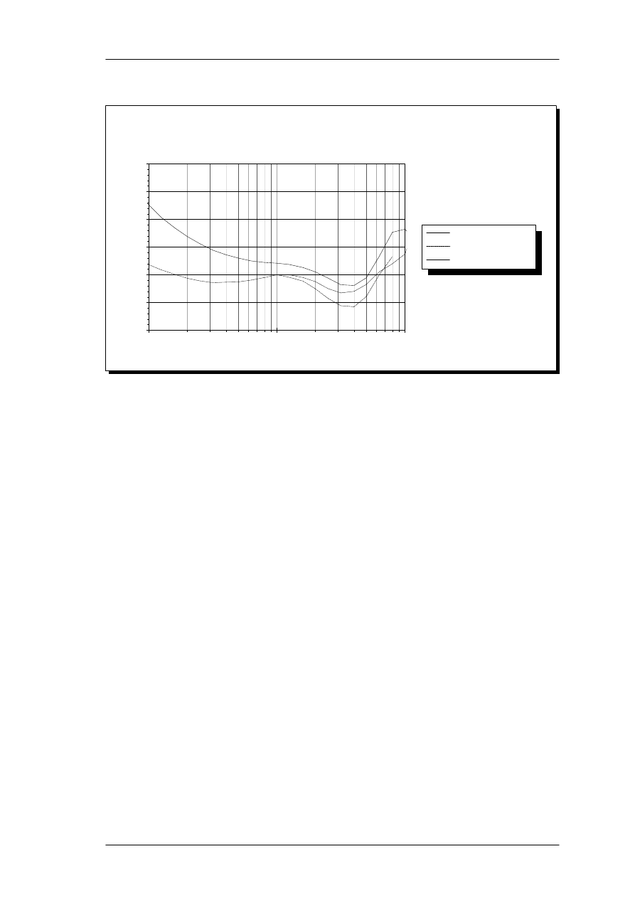
The shapes of the ELC-100 curves and a
0
curves are shown in Figure 2 along with the
ISO 226 (1987) curve for comparison.
Page 24
An auditory model with hearing loss.
3. Model description
Open ear binaural thresholds
and correction curves.
Frequency, Hz
dB SPL
-20
-10
0
10
20
30
40
100
1000
10000
MAF (ISO 226 - Bin)
100 phon (ISO 226) - 100 dB
a0 - attenuation.
2.
Various proposed threshold correction curves. The original minimum audible field curve (MAF)
and 100 phon Equal-Loudness Contour (shifted 100 dB down) are from ISO226. The a
0
curve used
by Zwicker assumes that the thresholds below 1 kHz are elevated due to internal physiological
noise in the cochlea, and that the transmission system itself has no attenuation below 1 kHz.
Glasberg and Moore (1990) use different corrections, depending on the sound delivery
system and the frequency range. A MAF correction is used in conjunction with a
free-field listening situation or a free-field equalized headphone, whereas a MAP
(Minimum Audible Pressure) correction is used with a transducer intended to produce a
flat frequency response at the eardrum (Killion, 1984). Given the non-parallel
equal-loudness contours, explained by the low-frequency internal noise in the cochlea,
the authors recommend using the 100-phon equal-loudness contour (ELC-100) instead
of MAF below 1 kHz. When used for derivation of filter shapes from notched-noise
masked threshold, this correction is also found to be the most appropriate (Moore and
Peters, 1990).
An important issue for model implementation is the choice of reference point, with two
obvious alternatives: In the free field (at the center of the head with the listener absent)
or at the tympanic membrane (TM), also referred to as the eardrum. The free field can
be considered a more physically well-defined point common to all subjects, whereas the
sound pressure level at the eardrum depends on individual variances in outer ear and ear
An auditory model with hearing loss.
Page 25
3. Model description

canal geometry and varying input impedance of the eardrum. The current model is
intended for use with hearing aids, where signals are not presented in the free field, but
rather at the eardrum or in an ear simulator (IEC 711, 1981). This points towards using
the TM as reference point. However, the choice must primarily be based on the
availability and reliability of psychophysical data. The largest amount of coherent data is
provided in the ISO 226 (1987) standard for normal-hearing subjects, listening
binaurally. Here, MAF data and equal-loudness contours are given for pure tones, and
these are used in the auditory model.
In the auditory model, the auditory thresholds for a subject are input as dB HL values
from the audiogram, as obtained on an IEC 303 (1970) coupler in standard audiometry.
These hearing level values are then converted to dB SPL (ISO 389, 1991) in the coupler
and then to equivalent free-field values, using the IEC303 - free field corrections
provided by Bentler and Pavlovic (1992). For a binaural listening situation, a threshold
correction must be subtracted. Killion (1978) suggests a monaural disadvantage of 2 dB,
while Berger (1981) suggests 3 dB. From a signal detection point of view, and assuming
that the threshold of hearing is equivalent of a noise floor and that the noise sources of
the two ears are uncorrelated, two detectors are equivalent to a 3 dB increase in
signal-to-noise ratio, and a corresponding drop in threshold value. Bentler and Pavlovic
(1989) use 1.5 dB at low frequencies, rising to 2.5 dB and 3.8 dB at 5 and 6 kHz,
respectively. In the current project it was decided to use a 3 dB flat correction, as was
also proposed by Scharf & Buus (1986), e.g. the binaural threshold power equals half the
monaural threshold power. At higher levels, power summation is not the important
factor, but rather loudness summation, so the monaural-binaural correction must be
made in the loudness domain (see section 3.5.1). In either case, the binaural model
assumes two completely identical ears, and the asymmetrical case is not accounted for.
As previously mentioned the output from a hearing aid is typically recorded in an ear
simulator (IEC 711, 1981), where the sound pressure level at the microphone represents
the level at the eardrum in an average ear. Consequently, this type of signal must be
weighted by a coupler correction frequency response, transforming it to equivalent
free-field values. The open-ear transfer function - from free-field to eardrum - has been
Page 26
An auditory model with hearing loss.
3. Model description

measured by Shaw (1974) and later presented in numerical form by Shaw & Vaillancourt
(1985). By subtracting Shaw's gain values from to the IEC 711 coupler spectra, the
equivalent free-field spectra are obtained as input to the model.
The MAF curve has a prominent dip from 1 to 8 kHz with a minimum at 4 kHz, which is
logically assumed to arise from the acoustic gain of the external ear and in particular the
ear-canal resonance. However, the open-ear transfer function (Shaw, 1974) has its peak
located at 2.6 kHz. By adding Shaw's data to the MAF curve, a threshold curve for the
sound pressure level at the tympanic membrane can be obtained. This is termed
Minimum Audible Pressure (MAP). Killion (1978) has derived MAP from MAF in this
manner. The MAP curve is not flat as would be assumed from the above hypothesis, but
exhibits a "hump" at 2500 Hz, where the open-ear transfer function is located. No clear
explanation for this hump has been offered by Killion, who suggests the
eardrum-to-basilar membrane transfer function as an explanation.
Another investigation of the open-ear transfer function (Mehrgardt & Mellert, 1977)
shows a broader peak around 3-4 kHz which is in better agreement with the dip in the
MAF curve. By adding MAF and this open-ear response, a somewhat smoother MAP
curve is obtained, with a dip at 1-1.25 kHz as the most prominent feature. This
frequency, is where the middle ear begins to attenuate the signal (Allen, 1985), which
could account for the sharp rise in the MAP curve beyond 1.25 kHz.
It turns out that most MAP data published in the literature are essentially derived from
the ISO 226 (1987) MAF data or other MAF measurements, based on an average
free-field to eardrum transfer function. The current model should therefore use the
free-field as reference, with three choices of equalization curves:
w The a
0
correction used by Zwicker & Feldtkeller (1967) and Zwicker & Fastl
(1990).
w The ELC-100 curve as proposed by Glasberg & Moore (1990).
w A combination of the two, where the ELC-100 curve is modified below 1
kHz to be flat.
An auditory model with hearing loss.
Page 27
3. Model description

When the model is then used with reference to the eardrum, or an IEC 711 ear simulator,
two MAF-MAP corrections are available:
w Shaw and Vaillancourt (1985), based on Shaw (1974).
w Mehrgardt & Mellert (1977).
It is also possible to convert signals recorded in an IEC303 (6 cm
3
) coupler, using the 6
cm
3
-free-field transformation proposed by Bentler and Pavlovic (1992).
3.4
Auditory filter bank.
The filter model originates from the work by Patterson, Moore, Glasberg and others
(Patterson et al, 1982; Moore & Glasberg, 1983, Tyler et al, 1984; Glasberg & Moore,
1986; Moore & Glasberg, 1987; Glasberg & Moore, 1990). The auditory filter model is
based on detection of pure-tone signals in symmetrical and asymmetrical notched-noise
maskers. The derivation of the filter shape is based on two assumptions: 1) The auditory
filter used for detection of the signal in the masker will be centered at the frequency
yielding the highest signal-to-masker ratio; 2) Detection threshold corresponds to a fixed
signal-to-masker ratio at the output of the filter, known as detection efficiency. Under
these assumptions, an analytical expression for the shape of the auditory filter can be
derived. The parameters in the filter expression can be determined for an individual by
means of the notched-noise masked thresholds.
Based on the auditory filter shape, excitation patterns for harmonic stimuli can be
calculated as the output of each filter in a filter bank (Moore & Glasberg, 1987). This
calculation model centers an auditory filter at each frequency component in the stimulus.
For implementation of a generalized auditory model, this concept must be modified, to
limit the number of channels and to obtain an acceptable processing speed. On the other
hand, a model with few filters at fixed center frequencies violates the first assumption of
the auditory filter model. The model should ideally focus on local or global peaks in the
power spectrum, or perhaps on local peaks in pre-defined frequency regions. Using this
Page 28
An auditory model with hearing loss.
3. Model description

approach, the entire auditory spectrum would be covered, while the auditory filters were
allowed to maximize signal-to-masker ratio locally
1
.
However, for convenience and subsequent interpretation by a neural network, the
current model uses a fixed number of channels at fixed center frequencies. When the
filter bandwidth increases as function of hearing loss (section 3.4.1) and level (section
3.4.2), the filters become overlapping, which is not a correct interpretation of the
auditory system. It should rather be modeled by a decreasing number of non-overlapping
filters. This is discussed further in section 3.5.2, and a correction for the widening filters
at fixed center frequencies is introduced.
The auditory filter shape W(g) is generalized by the function (Moore & Glasberg, 1986):
W
(
g
)=
(1
−
r)
(
1
+
pg
)
e
−
pg
+
r
(2)
This is the rounded exponential, roex(p,r), filter, with two parameters, the exponential
slope parameter, p, and the base level r. A high p indicates sharper tuning, and p is
affected by frequency, level in the band and by hearing loss. A typical value at 1 kHz and
low input levels for a normal-hearing listener is 20 - 25. The second parameter, r
determines the filter weight outside the passband, the stopband level. This is often highly
correlated to absolute threshold of hearing. g is the normalized distance from the center
frequency of the filter, f
c.
g
(
f
)=
f
−
f
c
f
c
(3)
The filter function, W(g), can also be thought of as a weight function applied to the
power spectrum of the stimulus. An example of the filter function is shown in Figure 3.
An auditory model with hearing loss.
Page 29
3. Model description
1
Since the spectrum of signal and masker cannot be estimated independently, we
make the assumption that a filter centered on a spectral peak yields the highest
signal-to-masker ratio.
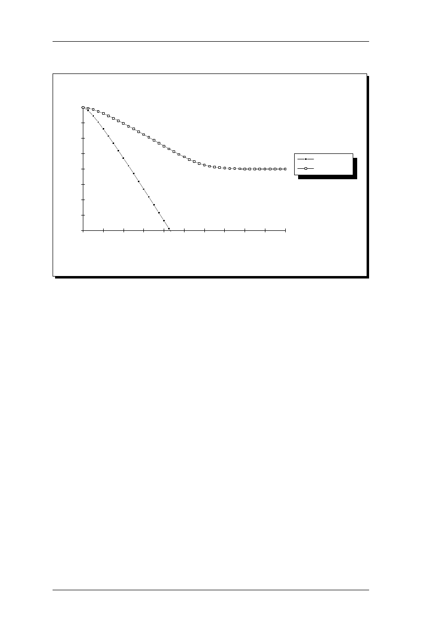
Roex filter shapes
g = (f-fc)/fc
Attenuation, dB
-80
-70
-60
-50
-40
-30
-20
-10
0
0
0.2
0.4
0.6
0.8
1
1.2
1.4
1.6
1.8
2
r = 0, p = 25
r = 0.0001, p = 10
3.
Sample plots of roex(p,r) filter shapes with different slopes, p, and tails, r.
The "tails" of the filter, characterized by r, appear to be linked to the absolute threshold
of hearing (Glasberg & Moore, 1986) and are thus omitted from the filter bank stage,
since the threshold function will be implemented in a later stage of the auditory model.
The simplified roex(p) filter equation used here is:
W
(
g
)= (
1
+
pg
)
e
−
pg
(4)
The p parameter determines the slopes of the filter and thus indirectly the bandwidth.
For moderate sound levels, the filter shape becomes asymmetrical, and p is allowed to
have different values on the two sides of the center, p
l
below f
c
and p
u
above f
c
. When
viewed on a linear frequency scale for constant p, the roex filters are symmetrical with a
widening bandwidth as center frequency increases. Viewed on a logarithmic frequency
scale, the filters are all the same width and asymmetrical. This is illustrated in Figure 4.
Page 30
An auditory model with hearing loss.
3. Model description
Roex filter shapes
f, kHz
Attenuation, dB
-80
-70
-60
-50
-40
-30
-20
-10
0
0.10
1.00
10.00
250 Hz
1 kHz
4 kHz
4.
Examples of three typical roex filter shapes at three center frequencies. The p values are the same
above and below the center frequency.
A digital filter model with logarithmically spaced center frequencies will thus be more
suited than an FFT-model with linearly spaced lines. The roex filter can be approximated
by a "gamma-tone" impulse response, as Moore et al (1989) have done in a paper on
temporal gap detection. This impulse response exhibits amplitude and phase response
similar to those derived from single neuron measurements in the cat. The result is a fixed
filter, independent of the signal power in that band, contrary to the general theory, that
auditory filters cause increased upward spread of masking with increasing level (Lutfi &
Patterson, 1984).
As an alternative and future improvement to the FFT-approach, a wavelet-based
filterbank with center-frequencies and bandwidths corresponding more closely to a
critical-band scale (Agerkvist, 1992) or an ERB-scale might be more correct. Such a
pre-processor would have high temporal resolution at high frequencies and low temporal
resolution (i.e. a long window) at low frequencies, as the auditory filterbank does, when
modeled as a series of simple resonators (de Boer, 1985).
An auditory model with hearing loss.
Page 31
3. Model description

The FFT-based model initially determines the power spectrum and subsequently corrects
the spectrum for external and middle ear transfer functions, as discussed in section 3.3.
Based on this corrected spectrum, which can be interpreted as the input spectrum to the
cochlea / filterbank, the parameters of the auditory filters can be adjusted. The adjusted
filters are then easily applied to the signal by multiplication in the frequency domain. A
disadvantage of the FFT-based model is the limited time resolution due to a block-based
analysis. With a sampling rate of 20 kHz, the time window is 12.8 and 25.6 ms for a
256- and 512-point FFT, respectively. A short-time FFT will also provide very poor
frequency resolution, wider than 78 and 39 Hz for the 256- and 512 point FFTs,
respectively. The degree of smearing in the frequency domain also depends on the
choice of window function.
Furthermore, phase information and time delays are not similar to a real ear, where a
cascade of IIR filters would provide a more realistic model due to the basilar membrane
traveling wave simulation (Lyon, 1982). Recent data (Moore & Glasberg, 1989)
indicate that the ear cannot detect phase shifts of single component in a harmonic
stimulus when phases of the components were randomized. For a speech signal it is
likely, that the power spectrum provides the major speech cues (Leijon, 1989), thus the
loss of correct phase information in a power spectrum method is acceptable. In the case
of other signals, phase sensitivity may be a concern, but the knowledge in this area is still
limited. Other power-spectrum-based methods are described by Cohen (1989) and
Hermansky (1990) - see section 2.4 for a summary.
Moore and Glasberg (1983) presented data from several authors on the equivalent
rectangular bandwidth (ERB) of the auditory filter as function of frequency in the range
0.1 - 6.5 kHz. These data were later extended (Glasberg and Moore, 1990) to cover the
range 0.1 to 10 kHz.
The ERB can be calculated as:
ERB
Hz
=
24.7(4.37f
c
+
1)
(5)
Page 32
An auditory model with hearing loss.
3. Model description

where ERB is the bandwidth in Hz, and f
c
is the center frequency of the auditory filter in
kHz. Based on this, a psychoacoustical scale, similar to the Bark scale (Zwicker &
Feldtkeller, 1967), has been derived by integrating the reciprocal of the critical-band
function. The ERB-rate, or E scale is related to frequency by:
E
=
21.4 log(4.37f
+
1)
(6)
where f is in kHz.
The inverse expression for calculating f as a function of E is:
f
=
10
E
21.4
−
1
4.37
(7)
Thus, an auditory filter bank with fixed center frequencies should have these evenly
distributed on an E-scale. The E-scale is valid in the range E = 3 to 35, corresponding to
center frequencies from 87 Hz to 9.65 kHz. This range should then be covered by 33
filters, for a fixed-center-frequency model, an appropriate channel number for subsequent
data processing by an artificial neural network. In order to model masked thresholds for
broad-band, white noise signals adequately, 2 channels/ERB are required (Buus, 1992),
i.e. 65 channels, but this will increase the complexity of the system and probably result in
a high degree of correlation between channels.
3.4.1 Filter shape as a function of level.
The low-frequency slope of the roex filter depends on the signal level in each band being
added to the filter output. With increasing signal level, the lower branch becomes more
shallow for normal-hearing subjects. By analyzing data for asymmetric notch-noise
maskers from several studies and collapsing these across center frequencies, Glasberg &
Moore (1990), have determined the following linear relationship between the slope
An auditory model with hearing loss.
Page 33
3. Model description

parameter p
l
below center frequency and the sound pressure level X, corrected for
external and middle ear transfer functions (section 3.3), in the band:
p
l
(
X, f
c
)=
p
l
(
51,f
c
)
−
0.38
p
l
(
51,fc
)
p
l
(
51,1k
)
(X
−
51)
(8)
where p
l(51,fc)
is the value of p
l
at that center frequency obtained at 51 dB SPL/ERB, and
p
l(51,1k)
is the value of p
l
at 1 kHz and a noise spectrum level of 30 dB SPL/Hz,
corresponding to 51 dB SPL/ERB at 1 kHz. The value of p
l(51,fc)
depends on the center
frequency, f
c
, and is calculated from the ERB, remembering that p
l(51,fc)
= 4f
c
/ERB, where
f
c
is in Hz. The valid range of levels for this equation is not clear, however one of the
cited studies (Lutfi & Patterson, 1984) has obtained data for spectrum levels from 20 to
50 dB SPL/Hz, corresponding to 41 - 71 dB SPL/ERB at 1 kHz. The data from these
studies has will not be presented separately in here, since the equation presented by
Moore and Glasberg (1987) includes unpublished data, and the level dependency
function thus relies on the final analysis in the follow-up paper by Glasberg & Moore
(1990).
The slope parameter above center frequency, p
u
, does not vary consistently with level
(Moore and Peters, 1990), but only with center frequency f
c
and equivalent rectangular
bandwidth, ERB:
P
u
(f
c
)
=
4000f
c
/ERB
(9)
where f
c
is in kHz and ERB is in Hz. The model for calculating filter shapes thus
determines the power in bands that are one ERB wide (eqn. 4) and subsequently sets the
filter slopes according to eqn. 8 and 9. For a high signal level in a band below center
frequency, the low-frequency slope widens, and will be weighted higher in calculating the
output of that roex filter. For a stationary stimulus, the effective response of a filter at
higher center frequency will have local peaks, where high-level components are, as
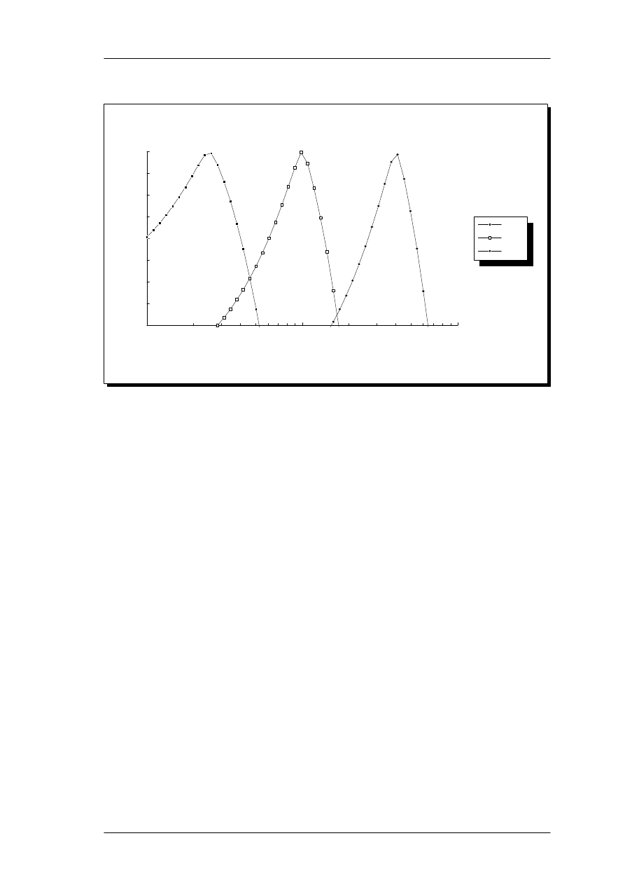
shown in Figure 5. This filter response does seem contrary to normal masking theory,
assuming monotonous filter functions. However, the significant feature of the model, the
Page 34
An auditory model with hearing loss.
3. Model description
derived excitation patterns generally assume the correct shape as indicated in Figure 13,
section 4.2.1.
Level dependent roex filter shapes
f, kHz
Power, dB SPL/ERB
40
45
50
55
60
65
70
75
80
85
1.00
1.46
2.14
3.14
4.59
6.73
9.85
-80
-70
-60
-50
-40
-30
-20
-10
0
Attenuation, dB
Signal ERB spectrum
Signal off
Signal on
5.
Effective roex filter shape at 4 kHz, when a 1 kHz pure tone signal is applied. The signal
decreases the filter slope, and is thus weighted higher. The resulting excitation patterns exhibit
increased upward spread of masking with increased level.
Since filter shape depends on the power passing through that filter, it might seem
obvious that the correct procedure for calculating the filter shape would be a series of
iterations, where the output power and the filter shape interacted. This would be a
feedback arrangement of filter shape and output power, as opposed to a feed-forward
model, where the input power is used to set the filter shape of the roex filter. Both
assumptions have been tested by calculating the excitation patterns for a 1 kHz sinusoid
at a range of levels (Moore & Glasberg, 1987), whereby only the input model
(feed-forward) produced the correct excitation patterns with increasing upward spread
of masking. For broad-band signals, on the other hand, strong components far from a
given filter should not be able to affect its shape, and an extension is proposed, where the
input power in one rectangular band, 1 ERB wide, is used to calculate the shape of that
An auditory model with hearing loss.
Page 35
3. Model description

particular filter channel. The calculation algorithm is listed in a FORTRAN program
(Moore & Glasberg, 1987), which was duplicated in the current model.
The level-dependent filter shapes are for normal-hearing subjects only. Since data were
collapsed to 1 kHz, the model is also based on the assumption that filter shape varies
with level the same way across all center frequencies. The authors emphasize, that more
data is needed to test this assumption.
Figure 12 (section 4.2.1) shows examples of excitation patterns from the model (i.e. filter
bank output) for various pure tones.
3.4.2 Filter shape as a function of hearing loss.
Glasberg & Moore (1986), measured auditory filter shapes for listeners with unilateral
and bilateral cochlear hearing impairments and found ERB and p
l
to be significantly
correlated with hearing threshold in dB SPL (on a B&K 4153/IEC 318 artificial ear) for
a 1 kHz pure tone stimulus. Additional data, including other frequencies, have later been
reported by Peters and Moore (1992) and Stone (1992). The data include unilateral and
bilateral losses of mixed origin (noise, presbycusis). In the current report, a model for
the filter shapes as function of cochlear (sensorineural) hearing loss has been determined,
based on further analysis of the published data.
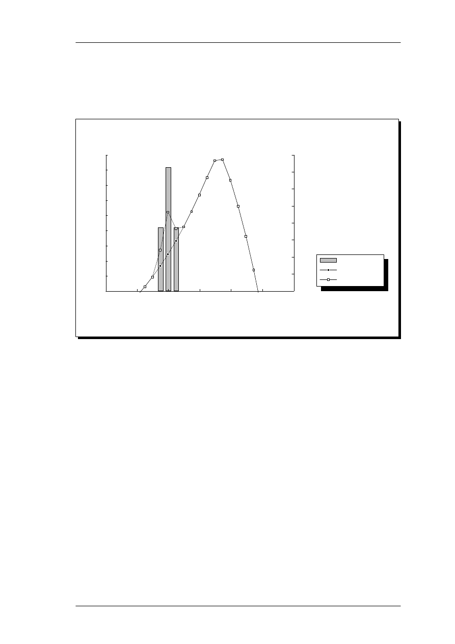
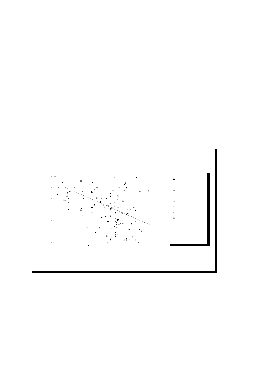
Glasberg & Moore (1986) found that the equivalent rectangular bandwidth (ERB) in
impaired ears increased for thresholds above 30 dB SPL, based on measurements at 1
kHz. With inclusion of additional data and by transforming all ERB values to a 1 kHz
equivalent, the data points for 137 filters on 50 ears can be plotted. This is shown in
figure 6.
Page 36
An auditory model with hearing loss.
3. Model description
Filter parameter ERB
transformed to 1 kHz
Threshold, dB SPL
ERB (kHz)
0.00
0.20
0.40
0.60
0.80
1.00
0
10
20
30
40
50
60
70
80
ERB(0.5) - ST92
ERB(1) - ST92
ERB(2) - ST92
ERB(4) - ST92
ERB(0.5) - G&M86
ERB(1) - G&M86
ERB(2) - G&M86
ERB(0.1) - P&M92
ERB(0.2) - P&M92
ERB(0.4) - P&M92
ERB(0.8) - P&M92
Normal (< 30 dB SPL)
Regr. line (>= 30 dB SPL)
ERB = -0.29 + 0.014*THR
6.
Equivalent rectangular bandwidth (ERB) plotted as a function of auditory threshold in dB SPL.
The data originate from Glasberg & Moore (1986), Peters and Moore (1992) and Stone (1992).
All values have been transformed to equivalent ERB at 1 kHz center frequency. The 0.1 and 0.2
kHz data were excluded prior to the regression analysis (see text).
It is clear, that there is a large spread of ERB values for a given threshold. As a simple
approximation and generalization, the current auditory model should predict the
rectangular bandwidth based on thresholds. Following the argument from Moore &
Glasberg (1986), that auditory filters are normal for thresholds below 30 dB SPL, a
linear regression analysis was performed on all data points above 30 dB SPL. At 0.1 and
0.2 kHz, however, the ERB-values are very scattered. The derivation of these filter
shapes is very sensitive to the low-frequency transfer characteristics of the transducer,
and show a large spread, even for normal-hearing listeners (Moore & Peters, 1990).
This is consistent with physiological results, showing that the low-frequency tuning
curves are very broad and poorly defined below app. 600 Hz in cats, corresponding to
300 Hz in humans (Evans & Elberling, 1982). The 0.1 and 0.2 kHz data points were
thus excluded from the analysis.
An auditory model with hearing loss.
Page 37
3. Model description

A linear regression analysis for thresholds above 30 dB SPL, excluding 0.1 and 0.2 kHz
data points, yields the following relationship at 1 kHz:
ERB
1k
(
THR
)= −
0.29
+
0.014
&THR ; THR m30.7 dB SPL
(10)
for thresholds in the range 31 to 70 dB SPL. Above this range, there is no data for
prediction of filter shapes, and practically no remaining frequency selectivity (Ludvigsen,
1985). Below this range the ERB is normal as expressed in eqn. 5 with correction for
level (see below). The regression analysis is similar to the analysis of Glasberg & Moore
(1986), who found a more shallow slope (0.0097). There is a modest and significant
correlation (r = 0.52, p < 0.0001), so the linear model was accepted. The ERB here is
expressed as proportion of center frequency, which at 1 kHz is equal to the filter
bandwidth in kHz.
The data might be better fit with a power- or exponential function, thus providing a
smooth transition from normal hearing to hearing loss. Furthermore, a data
transformation might provide a more constant spread of Y-values with increasing
threshold. For simplicity, however, a linear model was used in this and the following
analyses on change in filter shapes with threshold in dB SPL. This also allows for a
straightforward and meaningful introduction of level effects into the model, since the
level effects are also linearly dependent of dB SPL (section 3.4.3).
Consistent with summarized results from several studies (Tyler, 1986) auditory filters
broaden with increasing hearing loss, but there is a large spread around the general trend.
An alternative would be to specify the filter parameters on an individual basis, but this is
not included in the current implementation of the model. The regression suggested
above is always used. Leijon (1989) specifies typical values for widened filters for his
model, but it is unclear how these values are then interpolated between test frequencies
for each filter channel. His model is only used with a number of hearing loss cases and
not for any audiogram.
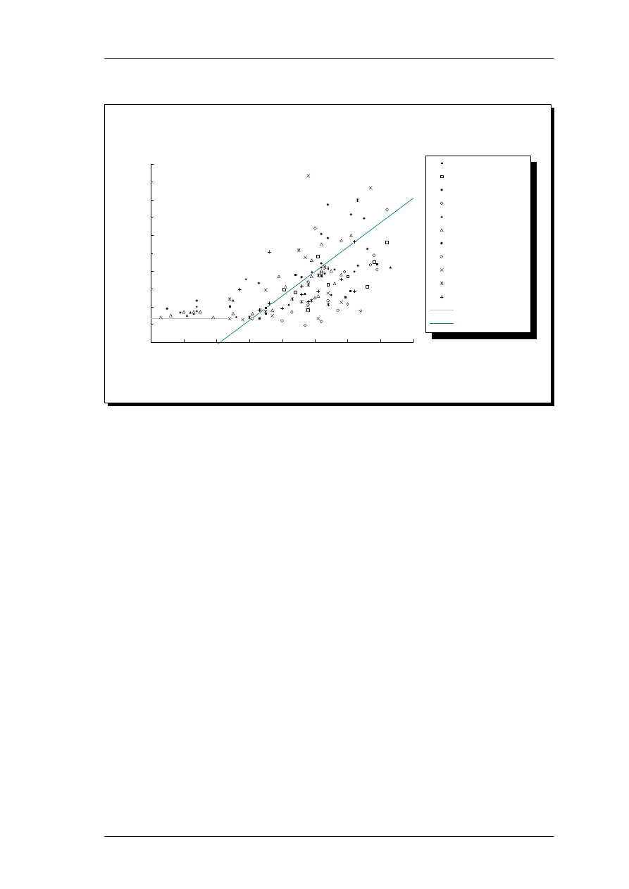
For the LF-slope (high-pass) as a function of threshold, p
l,
a scatter plot is shown in
Figure 7. There are certain data points that clearly do not fit the trend of decreasing
Page 38
An auditory model with hearing loss.
3. Model description
slope with increasing threshold. These are primarily data for low center-frequencies
(100, 200 Hz), where the filter fitting procedure tends to show larger variation across
individuals and is furthermore very sensitive to the type of threshold correction used
(Moore et al, 1990). The remaining data points can be approximated by a similar
piecewise linear function.
Filter parameter pl
transformed to 1 kHz
Threshold, dB SPL
pl
0.00
5.00
10.00
15.00
20.00
25.00
30.00
0
10
20
30
40
50
60
70
80
Pl(0.5) - ST92
Pl(1) - ST92
Pl(2) - ST92
Pl(4) - ST92
Pl(0.5) - G&M86
Pl(1) - G&M86
Pl(2) - G&M86
Pl(0.1) - P&M92
Pl(0.2) - P&M92
Pl(0.4) - P&M92
Pl(0.8) - P&M92
Normal (< 30 dB SPL)
Regr line (> 30 dB SPL)
Note: 0.1 and 0.2 kHz data points were excluded from regression analysis
pl = 28.09 - 0.33*THR
7.
The low-frequency filter slope parameter, p
l
, plotted as a function of auditory threshold in dB SPL.
The data originate from Glasberg & Moore (1986), Peters and Moore (1992) and Stone (1992).
All values have been transformed to equivalent values at 1 kHz center frequency. The regression
line was calculated after exclusion of the 0.1 and 0.2 kHz data, that showed very large spread.
Based on these selection criteria and using only points with thresholds above 30 dB SPL,
a regression analysis for p
l
transformed to 1 kHz yields:
p
l
(
1k, THR
)=
28.09
−
0.33
&THR ; THR m16.9 dB SPL
(11)
for thresholds in the range 16.9 to 70 dB SPL. No predictions are made above this
range. Since ERB, p
l
and p
u
are related (Glasberg & Moore, 1990), the regression
analysis should indicate intersections for identical threshold values (30.7 resp. 16.9 dB
SPL). The large spread of data points indicates that they could, in fact, intersect at the
An auditory model with hearing loss.
Page 39
3. Model description
same point, but without clear evidence, no modification of the analysis results was made.
The filter slope decreases with increasing hearing loss (r = -0.61, p < 0.0001). This is
consistent with the increasing ERB and furthermore leads to an increased upward spread
of masking (Tyler et al, 1984). A similar shallower slope on the low-frequency side of
psychoacoustical tuning curves has been observed by Florentine et al (1980). Even
though the model fitting was done without the 100 Hz and 200 Hz data points, it has
been extrapolated to cover these frequencies, based on the remaining data points.
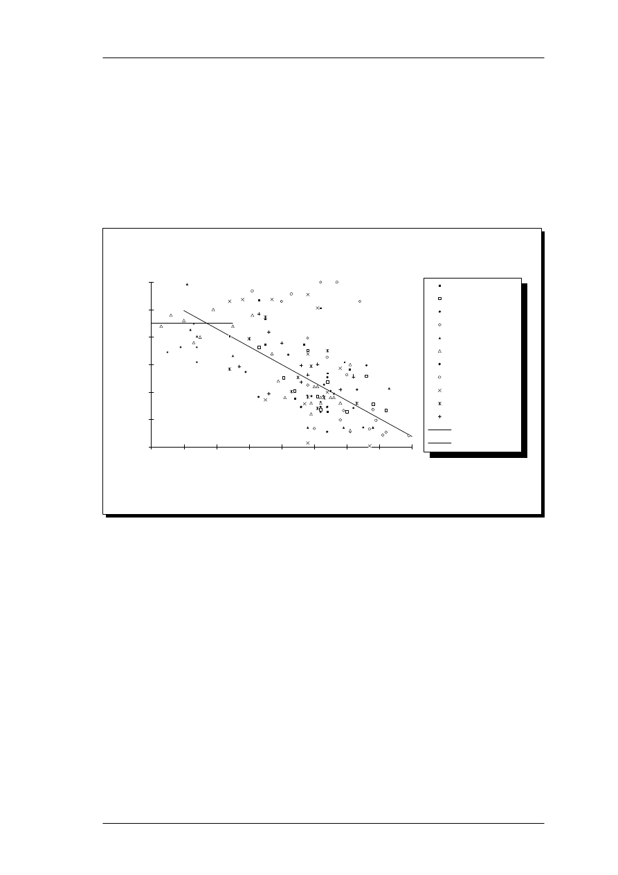
For the HF-slope (low-pass) as a function of threshold, pu has also been plotted as a
function of absolute threshold, as shown in figure 8. This plot has considerable scatter,
and no clear trend is evident.
Filter parameter pu
referred to 1 kHz
Threshold, dB SPL
pu
0.00
10.00
20.00
30.00
40.00
0
10
20
30
40
50
60
70
80
90
Pu(0.5) - ST92
Pu(1) - ST92
Pu(2) - ST92
Pu(4) - ST92
Pu(0.5) - G&M86
Pu(1) - G&M86
Pu(2) - G&M86
Pu(0.1) - P&M92
Pu(0.2) - P&M92
Pu(0.4) - P&M92
Pu(0.8) - P&M92
Reg line (>30 dB SPL)
Normal = 30.2
8.
The high-frequency filter slope parameter, p
u
, plotted as a function of auditory threshold in dB
SPL. The data originate from Glasberg & Moore (1986), Peters and Moore (1992) and Stone
(1992). All values have been transformed to equivalent values at 1 kHz center frequency.
There seems to be a weak tendency of a decreasing slope with increasing hearing loss
corresponding to increased downward spread of masking with level, although the data
show a dubious correlation (r = -0.36, p < 0.08) for thresholds above 30 dB SPL. In line
Page 40
An auditory model with hearing loss.
3. Model description

with this result, Florentine et al (1980) found no systematically increasing downward
spread of masking with hearing loss. Due to the filter-fitting process, the value of p
u
is
not well defined when the value of pl is much smaller (Glasberg & Moore, 1986), which
can serve as a partial explanation of the large spread of data points.
Based on these considerations, the value of p
u
was kept constant (= normal hearing) in
the model, and only increased upward spread of masking with hearing loss was included.
The auditory filter shape in hearing-impaired subjects may be highly variant, even normal
auditory filter can be found (Tyler, 1986). The data used for the present analysis show
significant spread. However, the present model is accepted as a reasonable
approximation with interpolation of filter shapes to other frequencies. A correction was
required, since all thresholds in the original data were expressed as absolute thresholds in
dB SPL on a B&K 4153 artificial ear (IEC 318). The audiogram, expressed in dB HL
was thus converted to dB SPL using ISO389 (1991) for the IEC 318 coupler.
3.4.3 Filter shape as a function of level and hearing loss.
In the current auditory model, the level and hearing loss effects mentioned above should
be combined in a meaningful way, that corresponds with experimental results.
In section 3.4.1 filter shapes as function of level for normal-hearing listeners were
discussed. Since no similar data has been published for hearing-impaired listeners, the
initial assumption is to add the two effects in some fashion. Florentine et al (1980)
conclude that cochlearly impaired listeners show reduced frequency selectivity compared
to normal listeners at equal absolute levels (dB SPL). The masking model described by
Ludvigsen (1985) demonstrates decreasing masking slope with increasing level. The
masked threshold is then further modified by hearing loss, i.e. level and hearing loss (<
70 dB HL) are both leading to reduced frequency resolution.
A recent investigation by Dubno and Schafer (1992) led to a similar result. In their study
the absolute thresholds of hearing impaired subjects were simulated in normal-hearing
subjects by means of a shaped broad-band noise. The masked thresholds obtained with
An auditory model with hearing loss.
Page 41
3. Model description

both a notched-noise masker and a narrow-band masker were measured at identical
Sensation and Sound Pressure Levels due to the simulated hearing loss. Under these
equal conditions, the hearing-impaired subjects still had reduced frequency selectivity.
From the notched noise masked thresholds, p (assuming symmetric filters) and ERB
values were derived (Patterson et al, 1982) - with p values below those of the simulated
hearing losses, and ERB values were similarly higher than for the masked normal-hearing
listeners. For the hearing-impaired listeners, the presented graphs indicate that masked
threshold slopes decrease with increasing level, however this is not discussed in the
paper, and the level effect in hearing-impaired listeners may be dubious.
The first level and loss effect, Alternative 1, is that the model should combine the effects
of level and hearing loss, even at high levels. The level dependency effect for p
l
(Glasberg and Moore, 1990) is based on a masker spectrum level of 30 dB SPL/Hz (51
dB SPL/ERB at 1 kHz), whereas the hearing loss effect is based on a spectrum level of
50 dB SPL/Hz (71 dB SPL/ERB at 1 kHz). The regression line is essentially the same,
but levels are referred to 71 dB SPL/ERB instead. Furthermore the values are modified
by frequency. Combining all of this, we get a set of equations, where ERB is the
equivalent rectangular bandwidth in kHz, f
c
is the band center frequency in kHz, X is the
sound pressure level in one E band, and THR is the audiogram threshold in dB SPL,
measured in an IEC 318 artificial ear:
ERB
(
f
c
, THR
)=
4.37f
c
+
1
5.37
(
−
0.29
+
0.014
&max
(
30.7, THR
)
)
(12)
For the low-frequency slope, p
l
, as function of frequency, level and hearing loss, the
formula for Alternative 1 becomes:
p
l
(
f
c
, X, THR
)=
5.37f
c
4.37f
c
+
1
(28.09
−
0.33
&max
(
16.9, THR
)−
0.38
(
X
−
71
)
)
(13)
Page 42
An auditory model with hearing loss.
3. Model description

Based on the vague results on level and loss effects on the high-frequency slope
parameter, p
u
, it was decided to make it a function of center frequency, f
c
, only:
P
u
(f
c
)
=
161.94f
c
4.37f
c
+
1
(14)
It was decided to limit hearing thresholds to 70 dB SPL, and levels to the range 20 - 100
dB SPL/ERB, since psychophysical data is not available outside of these ranges. The
auditory model assumes constant values outside the ranges equal to the values at the
limits.
Alternative 2 assumes level dependency only at normal hearing (here defined as
thresholds below 20 dB SPL, the cutoff-point for the p
l
regression curve). Here, the
level and threshold effects have been combined in a more logical way: There are no level
effects at thresholds above 20 dB SPL. For lower thresholds, the tuning is increased
with decreasing levels, down to a cut-off point, which depends on threshold. This means
that for a normal hearing threshold, there is a 20 dB range at the bottom with increasing
tuning, similar to a fully functional cochlear amplifier. This is shown schematically in
figure 9 for a number of hearing losses. Below 51 dB SPL/ERB, there is no further
increase in filter slope. In this manner, the tuning enhancement is active only at low
levels combined with little or no hearing loss. The combination of effects was done by
using the intersect and slope values corresponding to the level effect, with only a slight
decrease in goodness of fit. The effect presented here shows sharper tuning when the
hearing thresholds are normal (< 20 dB SPL) and the signal power is low, as was also
reported by Peters and Moore (1992).
An auditory model with hearing loss.
Page 43
3. Model description
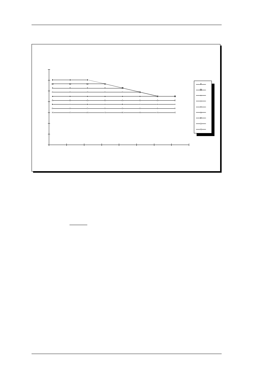
Model of pl as function of
level and hearing loss
Level, dB SPL/ERB
pl
0
5
10
15
20
25
30
35
40
45
50
55
60
65
70
75
80
0
5
10
15
20
25
30
35
40
Hearing loss
dB HL
9.
Schematical representation of the level dependent increase in filter slope for low thresholds (< 20
dB SPL) and low levels (< 71 dB SPL/ERB) as described in Alternative 2. For normal hearing,
the bottom 20 dB show increased tuning with decreased levels.
The formula for Alternative 2 is:
p
l
(
f
c
, X, TH
)=
5.37f
c
4.37f
c
+
1
(30.16
−
0.38
&
(
max
(
min
(
0, X
−
71
)
, TH
−
20
)+
20
)
)
(15)
The approach used to modify and fit this alternative was not to use an empirical
statistical procedure, such as multiple regression, but rather to carefully modify the
known models (Moore and Glasberg, 1987 and Glasberg and Moore, 1990), hereby
preserving the larger bulk of data and knowledge that has evolved.
Page 44
An auditory model with hearing loss.
3. Model description
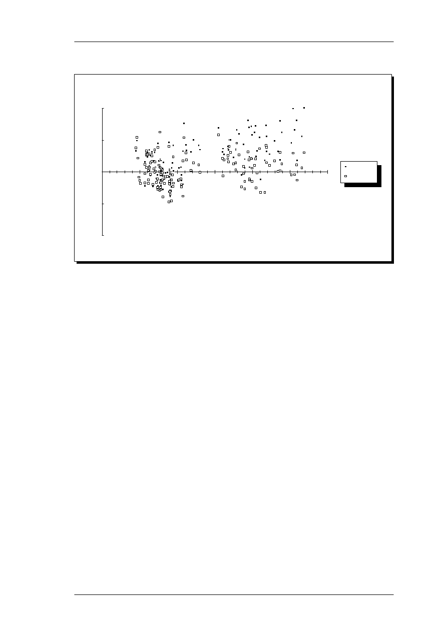
Residual pl vs. input level
Level, dB SPL/ERB
-20.00
-10.00
0.00
10.00
20.00
60.00
70.00
80.00
90.00
100.00
110.00
120.00
Alternative 1
Alternative 2
10.
Residual (actual - predicted) low-frequency filter slope parameter, p
l
, plotted as a function of
masker level in one auditory filter, where the ERB has been broadened by hearing loss. Residuals
are shown for two alternatives, 1) threshold and level in addition, and 2) no level effect for
thresholds > 20 dB SPL.
It is clear from Figure 10, that Alternative 2 fits the data better, with residuals spread
roughly symmetrically around the abscissa. Furthermore, the residuals of p
l
vs. hearing
loss (not depicted) are more evenly spread.
As described in Moore and Glasberg (1987), the filter slopes are adjusted according to
the summed energy in each E-band. With the combined loss and level effect, the ERB is
widened due to hearing loss, thus containing more energy. Consequently, the filter
slopes (p
l
, p
u
) are reduced, and reduced further due to the hearing loss. Effectively, the
hearing loss has been included twice in the model. However, with Alternative 2, this has
no effect, since ERB's stay normal up to 31 dB SPL, at which point the level-dependency
of the filter slope is no longer present.
An auditory model with hearing loss.
Page 45
3. Model description

3.5
Loudness function.
3.5.1 As a function of level and threshold.
As described in section 3.3, the shape of the normal hearing threshold curve can be
explained by a linear term, evident from the parallel parts of the equal loudness contours
and a threshold term that causes non-parallel curves at low levels. In the case of hearing
loss, the threshold curves will be shifted up vertically (expressed in dB SPL), but the 100
phon curve, for instance, may be unaltered compared to the normal-hearing case. The
loudness of a tone will thus rise to the same value, but within a much smaller dynamic
range.
One possible explanation for this abnormal loudness growth function (recruitment) for
impaired hearing are the broader excitation patterns, where the area of the pattern
expresses loudness (Evans, 1975b). This hypothesis was not confirmed by Florentine
and Zwicker (1979), who found that both recruitment and abnormal spread of masking
had to be added to their loudness summation model to explain experimental loudness
data. Other results with loudness matching in unilaterally impaired listeners (Moore et
al, 1985) support these findings. The authors present the hypothesis, that loudness is
encoded by means of nerve fibers with different thresholds, i.e. low-intensity and
high-intensity fibers. An impaired ear should then show recruitment due to loss of
low-intensity fibers. Simple experiments with the present auditory model also indicate
that broader excitation patterns alone do not account for recruitment. However, the
broadening of a fixed number of filters, causing them to overlap, requires some sort of
'normalization', for instance based on the rationale that the excitation at one point on the
basilar membrane is picked up by a fixed number of hair-cells (Leijon, 1989) - see section
3.5.2.
A separate loudness growth function incorporating the absolute threshold must thus be
formulated. Zwicker and Feldtkeller (1967) have described a model for loudness growth
in critical bands, termed specific loudness (N'). The model calculates loudness in each
Page 46
An auditory model with hearing loss.
3. Model description
critical band (1 Bark wide bands) from the excitation pattern. Total loudness, N, is then
formed as the integral of specific loudness versus critical-band rate.
N
=
°
z
=
0
24 Bark
N
Â
(
z
)
dz
(16)
In practical applications, the integral is substituted by a summation across bands. The
model is similar to Stevens' power law for high excitation levels, with a correction near
the threshold of hearing. The loudness growth function depends on the threshold in
quiet, which is interpreted as an internal noise source. The specific loudness equation for
1 kHz is presented by Zwicker & Fastl (1990), but the more general formulation of it
comes from Zwicker & Feldtkeller (1967). Here, a frequency-dependent detection term
is included, s, which is the ratio between the intensity of a just-audible test-tone and the
intensity of the internal noise appearing within one critical band around the test-tone.
N
Â
=
N
0
Â
E
TQ
sE
0
0.23
(
1
−
s
)+
sE
E
TQ
0.23
−
1
(17)
Here, N'
0
is a scaling constant, s is a detection factor, E is the excitation in the channel
caused by the input signal, E
TQ
is the excitation at threshold, and E
0
is the excitation for 0
dB SPL.
The constant N'
0
, is adjusted to meet the boundary condition, that 40 dB SPL at 1 kHz
should produce 1 sone as total loudness. At 1 kHz and for a fixed s = 0.5 (moved out
from the first set of brackets), the value should be 0.08 (Zwicker & Fastl, 1990) in
conjunction with a critical band scale, whereas the value 0.084 has been suggested by
Moore & Glasberg (1986) when an ERB-scale filterbank is employed.
The factor s indicates the signal-to-noise ratio required to detect the tone. By letting s
vary with frequency (Zwicker & Feldtkeller, 1967), the model is generalized to other
frequencies. This factor ("Schwellenfaktor" - Zwicker & Feldtkeller (1967), Bild 39,4) is
shown graphically and can be approximated as a piecewise linear function in a coordinate
An auditory model with hearing loss.
Page 47
3. Model description

system with dB and logarithmic frequency axes. This expression is converted from dB
by taking the antilog, and we thus get:
s
=
10
(
−
2
−
2.2 log
(
max
(
f/0.32,1
))
)/10
(18)
where f is the frequency in kHz. With an adjustable s, this must be included in the first
bracket term of eqn. (17), and N
0
' is instead set to 0.068 (Zwicker & Feldtkeller, 1967).
In the specific loudness equation (17), E
TQ
is the excitation at threshold in quiet, which
can also be interpreted as internal masking noise, and E
0
is the excitation that
corresponds to 0 dB SPL. These variables need to be set in the model, in order to
calculate specific loudness. In the current implementation, these two quantities are
calculated by passing a complex of pure tones, with one tone centered in each band. To
set E
0
, a 0 dB SPL pure tone is used in each channel and to set E
TQ
, the tones are set at
the hearing threshold level (dB SPL, interpolated in a dB - E coordinate system identical
to the perceptual frequency scale of the model). This approach has limitations, since it
simulates simultaneous presentation of several pure tones, instead of separate
presentation as in a hearing test. The advantage of avoiding the band interaction is, that
initialization is relatively fast. For high threshold levels, there may be a considerable
widening of the model filters, thus obtaining a very high threshold excitation. The
resulting loudness growth curve have elevated thresholds compared to the actual
thresholds. Therefore, the widening of the filters with hearing loss is disabled during
initialization, and the resulting loudness growth curves are properly aligned with the
thresholds. For subjects with very poor frequency selectivity, this approach may be
incorrect.
Since specific loudness is a power function, it should approach a straight line in a log-log
coordinate system. This is shown in Figure 11, for 6 levels of threshold excitation, 0 - 50
dB in 10dB steps. The asymptote for high excitation levels is a power law with exponent
0.23. The loudness growth model was originally based on stationary sounds, but it is
Page 48
An auditory model with hearing loss.
3. Model description
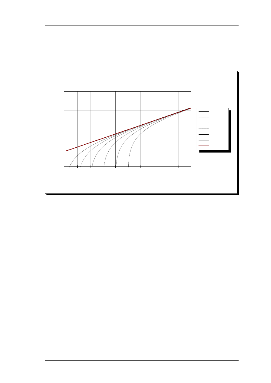
applicable to fluctuating signals as well (Zwicker & Terhardt, 1979) as in the present
model.
Idealized Loudness growth curves, 1 kHz pure tone
Excitation level, LE (dB)
Specific Loudness, N'
0.01
0.1
1
10
100
0
10
20
30
40
50
60
70
80
90
100
THR = 0
THR = 10
THR = 20
THR = 30
THR = 40
THR = 50
Exponent 0.23
11.
Theoretical growth of specific loudness for various thresholds as a function of
excitation, E in the auditory filter channel. Also shown is the asymptotic line
(E/E
0)
0.23
.
If a cochlear hearing loss can be simulated by normal hearing plus masking noise, the
above should represent impaired hearing as well. The current model thus appears
reasonable, and the loudness growth curve is qualitatively correct (Scharf, 1978a).
Other data available are individual equal loudness contours for hearing-impaired subjects
with sloping high-frequency losses from Lippman et al (1981) and Barfod (1976). The
loudness growth function for abnormal thresholds can be derived from these data under
the assumption that loudness growth is normal at low frequencies. However, these data
are all for individual subjects and are thus difficult to use for a general model.
Group results for the loudness growth function in hearing-impaired listeners have been
provided by Hellman and Meiselman (1990). Loudness growth functions were obtained
for 100 hearing-impaired listeners (primarily bilateral, noise-induced losses) by means of
absolute magnitude estimation (assigning a number to the perceived loudness), absolute
An auditory model with hearing loss.
Page 49
3. Model description
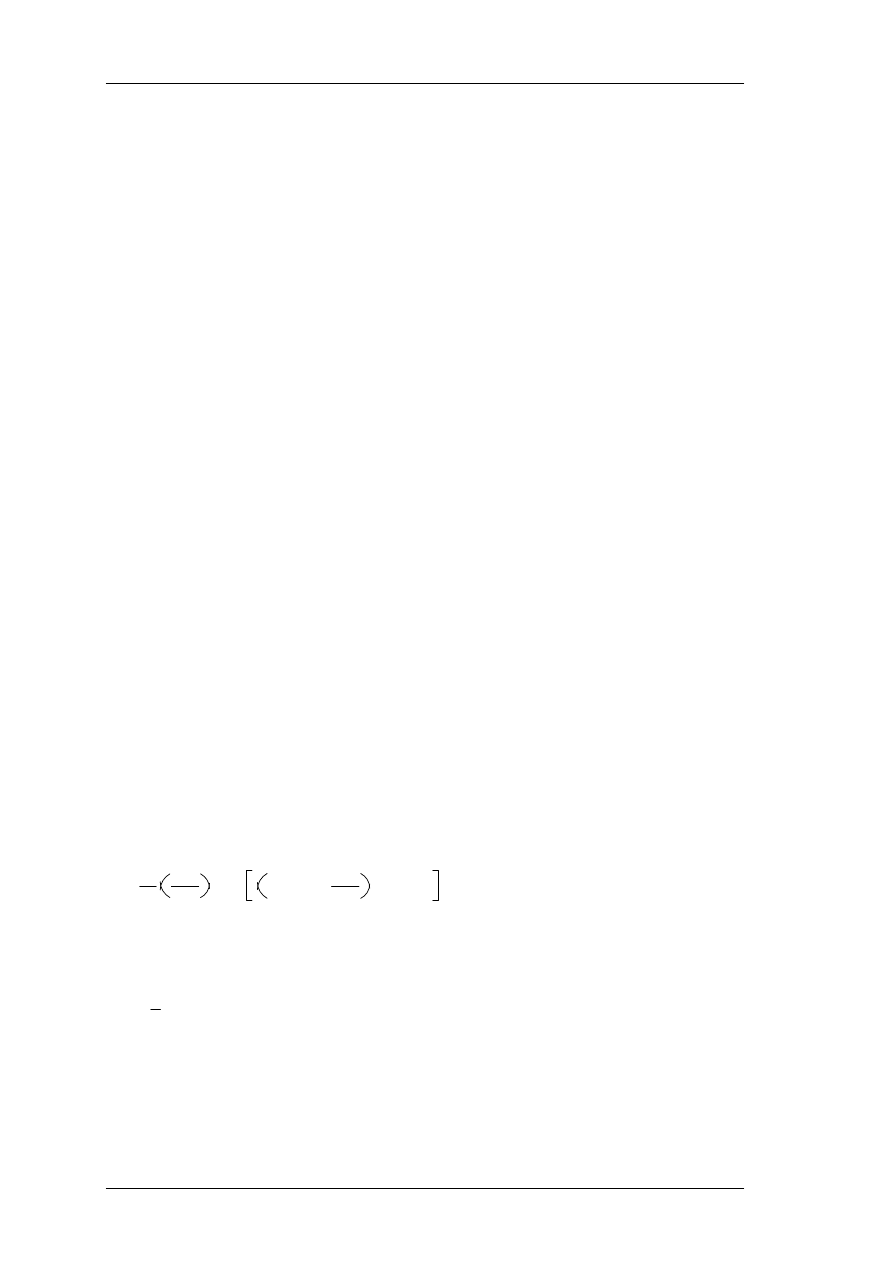
magnitude production (adjusting the level of a tone to match an assigned number) and
cross-modality matching (adjusting the level of a tone to match the perceived length of a
line on a screen). These data were well fitted by a power function (Zwislocki, 1965),
that subtracts the loudness of the internal masking noise (equivalent power of the
threshold raised by the exponent 0.27) from the loudness of the summed power of tone
and internal masking noise. This model is qualitatively identical to equation 17, which
can be seen by rearranging the terms in equation 17.
The theoretical models presented here are based on a binaural listening situation, and
must be modified for the monaural situation. At high levels, the binaural loudness
corresponds to an increase in monaural signal level by 10 dB, corresponding to a
doubling of loudness (Humes & Jesteadt, 1991). This simply implies that binaural
loudness is a simple addition of the loudness from each ear. Other results indicate that
loudness is increased by a factor between 1.7 and 2 (Scharf & Houtsma, 1986). The
current model uses a simple summation, but assumes two completely identical ears. The
asymmetrical case is not included in the model. Close to threshold, where detection is
the main effect rather than loudness rating, the loudness growth curve is much steeper.
The binaural detection threshold is improved by 3 dB (i.e. half power) as in two power
detectors with correlated input signals and uncorrelated background noise. This
corresponds to a doubling in loudness on the steep section of the curve (Scharf & Buus,
1986). Equation 16 can then be modified to monaural loudness by halving the loudness
and using the monaural threshold excitation, ETQM:
N
Â
=
N
0
Â
2
E
TQM
sE
0
0.23
(
1
−
s
)+
sE
E
TQM
0.23
−
1
(19)
In the binaural case, we then use the binaural threshold excitation instead:
E
TQ
=
1
2
E
TQM
(20)
Loudness near the uncomfortable level (UCL) is an important aspect of the model, since
loudness discomfort and output limiting are common and critical issues in hearing aid
fitting. Assuming that pure-tone UCL data is available for a subject, the model could
Page 50
An auditory model with hearing loss.
3. Model description

also somehow encode UCL, either as a separate output or as a different loudness value.
A proposed encoding of UCL is presented in Appendix 8.2, with the loudness value
rising steeply near UCL. This encoding has not been evaluated further.
For high sound levels, the acoustic reflex in the middle ear introduces a
frequency-dependent attenuation of the incoming sounds, primarily for low frequencies.
This will modify the input spectrum and thus the level-dependent masking effects and
decrease loudness. The current model does not include acoustic reflex.
3.5.2 Loudness summation in hearing-impaired listeners.
The model structure originates from the normal ear, with 33 channels representing the 33
auditory filters that are present when listening to broad-band sounds. In the impaired
ear, the broadened filters are fewer with larger spacing along the basilar membrane. In a
fixed channel model, the broadening of the auditory filters causes them to overlap, and
the same energy or 'excitation' is included more than once in the summed loudness. A
physiological interpretation is that the excitation at one point on the basilar membrane is
picked up by a fixed (but reduced due to hearing loss) number of hair-cells (Leijon,
1989).
In Zwicker's loudness model, the total loudness is formed by an integration of specific
loudness along the critical-band rate (Bark) scale (eqn. 16), which in a fixed channel
model can be approximated by a sum of the specific loudness contributions from each
filter channel:
N
=
S
i
=
0
24 Bark
N
Â
(
i
)
(21)
Leijon (1989) modifies the specific loudness by a filter widening factor that is specified
for a given subject. To make the loudness model simulate recruitment correctly, i.e.
normal loudness at high levels, the power-law exponent is also modified (not constant
0.23).
An auditory model with hearing loss.
Page 51
3. Model description

In the present model, the filter bandwidth increases with hearing loss as given by
equation 12, which can be used to compensate the loudness summation. Modifying to an
ERB-rate scale, we get:
N
=
S
i
=
0
N
ERB
N
Â
(
i
)
ERB
NH
ERB
HI
=
S
i
=
0
N
ERB
N
Â
(
i
)
−
0.29
+
0.014
&30.7
−
0.29
+
0.014 max
(
30.7,THR
)
(22)
This formulation preserves the original properties of the Zwicker & Fastl model. If this
is not sufficient, the next step would be to modify the power-law exponent. The
loudness growth function for normal and impaired hearing is evaluated in 4.3.1.
3.6
Temporal processing.
The current model is power-spectrum based and no attempt has been made to model
temporal processing, such as temporal integration or forward and backward masking.
The spectrally-based model will most likely disregard much of the fine-grain temporal
structure of speech, considered important for speech recognition. For estimation of
sound quality, however, spectral information may be adequate. Temporal processing was
thus considered a secondary factor, and within the time limits of the project, it was not
possible to implement and verify temporal factors in the auditory model.
Page 52
An auditory model with hearing loss.
3. Model description

4.1
Test design and stimuli.
The auditory model has been tested using a number of test stimuli (signals). All synthetic
signals were generated using the HyperSignal Workstation signal processing package
and stored in its .TIM time series format. Shaped noise was made from white noise by
convolving with a filter designed with the FILTSPEC program (ODIN, 1988). The
convolution was done using the CONVOL program (Nielsen, 1992).
Each model test session uses the AUDMOD.EXE program with a unique parameter text
file in the special file format required (see appendix 8.1 for an example and explanation).
4.2
Frequency selectivity.
The frequency selectivity in the literature is often characterized as either masking
patterns for narrow- or broadband stimuli, which are roughly equivalent of excitation
patterns. The difference between excitation and masking pattern depends on the
detection threshold of the probe signal in the masker within a given critical band.
Typically, the power of the pure tone is a few dB below the power of the masking noise
in one critical band. This is equivalent of the factor s (section 3.5.1 and Zwicker & Fastl,
1990), which varies with frequency, or the constant K factor deduced by Pavlovic (1987)
from Zwicker's data.
4.2.1 Excitation patterns, pure tones.
To illustrate the model behavior, the excitation patterns have been plotted for two pure
tones at increasing input levels. The excitation pattern is the output of the model across
channels. The physiological equivalent of this is the basilar membrane vibration pattern
along the place dimension. Examples of excitation patterns for 0.5 and 4 kHz pure tones
are shown in Figure 12, along with the quiet (threshold) excitation. The area between
the pure tone excitation pattern and the threshold excitation determines the loudness of
4
Verification.
An auditory model with hearing loss.
Page 53
4. Verification
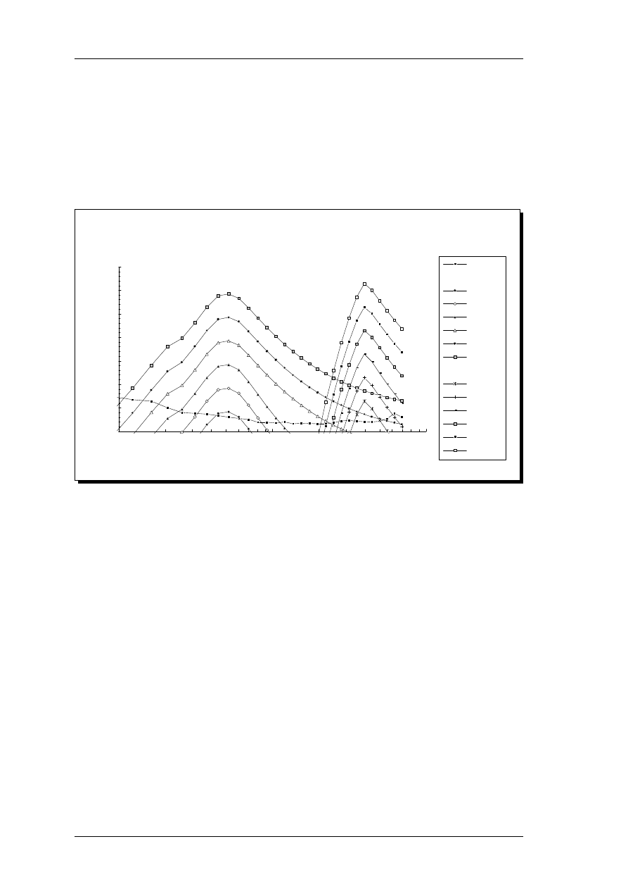
the stimulus. It is clear from the figure, that the tails of the 4 kHz patterns are missing,
thus leading to a low estimate of loudness, in particular at high levels, where a large area
is missing. This problem can be alleviated by using the model with a higher input
sampling rate and a higher upper frequency limit.
Excitation patterns, pure tones
Monaural, Normal hearing
f, kHz
Le, dB
0
20
40
60
80
100
120
140
0.1
1
10
Threshold
500 Hz:
20 dB SPL
40 dB SPL
60 dB SPL
80 dB SPL
100 dB SPL
120 dB SPL
4 kHz:
20 dB SPL
40 dB SPL
60 dB SPL
80 dB SPL
100 dB SPL
120 dB SPL
12.
Pure tone excitation patterns for 0.5 and 4 kHz pure tones at various levels compared to the
threshold excitation. The tails of the 4 kHz patterns are missing due to the upper frequency limit
in the model at 7 kHz.
For a 1 kHz pure tone at various levels, masking patterns have been presented by
Zwicker and Fastl (1990). These experimental pure tone masking patterns are irregular
close to the masker frequency and multiples of it, due to detectable beats between the
masker and the probe tone. These beats are detected by the subject, and the normal
masked threshold becomes difficult to obtain. The auditory model does not account for
beats, due to its power-spectrum foundation. Thus, it seems reasonable rather to
compare the model pure-tone excitation patterns with masked thresholds for a
narrow-band noise signal. The noise signal has a bandwidth less than one critical band (<
1 Bark), to excite only one auditory filter. This comparison of model excitation patterns
with narrow-band noise patterns is shown in Figure 13. The masked thresholds were
Page 54
An auditory model with hearing loss.
4. Verification
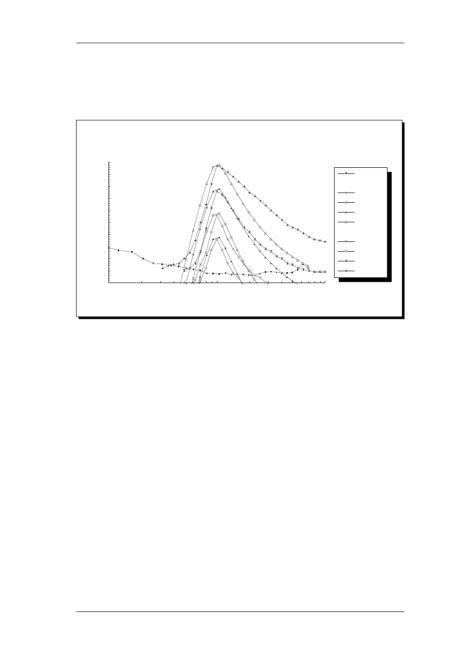
read off a graph (Zwicker & Fastl, 1990, Fig. 4.4) and entered in a spreadsheet, resulting
in not perfectly smooth curves.
Model excitation patterns
vs. experimental data.
f, kHz
Le, dB - Lt, dB SPL
0
10
20
30
40
50
60
70
80
90
100
0.1
1
10
Threshold
Model:
40 dB tone
60 dB tone
80 dB tone
100 dB tone
Experimental:
40 dB Noise
60 dB Noise
80 dB Noise
100 dB Noise
13.
A comparison of model excitation patterns for pure tones and masked thresholds for
critical-bandwide noise (Zwicker & Fastl, 1990, Fig 4.4). L
e
is the internal model excitation, and
L
t
is the level of the just-detectable test tone.
For low signal levels, the model curve coincides well with the masked thresholds. At
most levels (60-80-100 dB SPL), the model output extend further below the masker
frequency than the masked thresholds patterns. Thus, the two sets of experimental
thresholds are not identical, despite both being within the limits of one critical band. At
high levels (80-100 dB SPL), the masked threshold patterns have more shallow slopes
than the auditory model. This may be due to the upper limit for increasing filter
bandwidth in the model, at 71 dB SPL/ERB (see Figure 10), apparent from the parallel
curves at 80 and 100 dB SPL. An increase of this limit could be considered, however
this would also require an increase of the upper limit for hearing loss with enhanced
tuning at low levels (Figure 9).
An auditory model with hearing loss.
Page 55
4. Verification
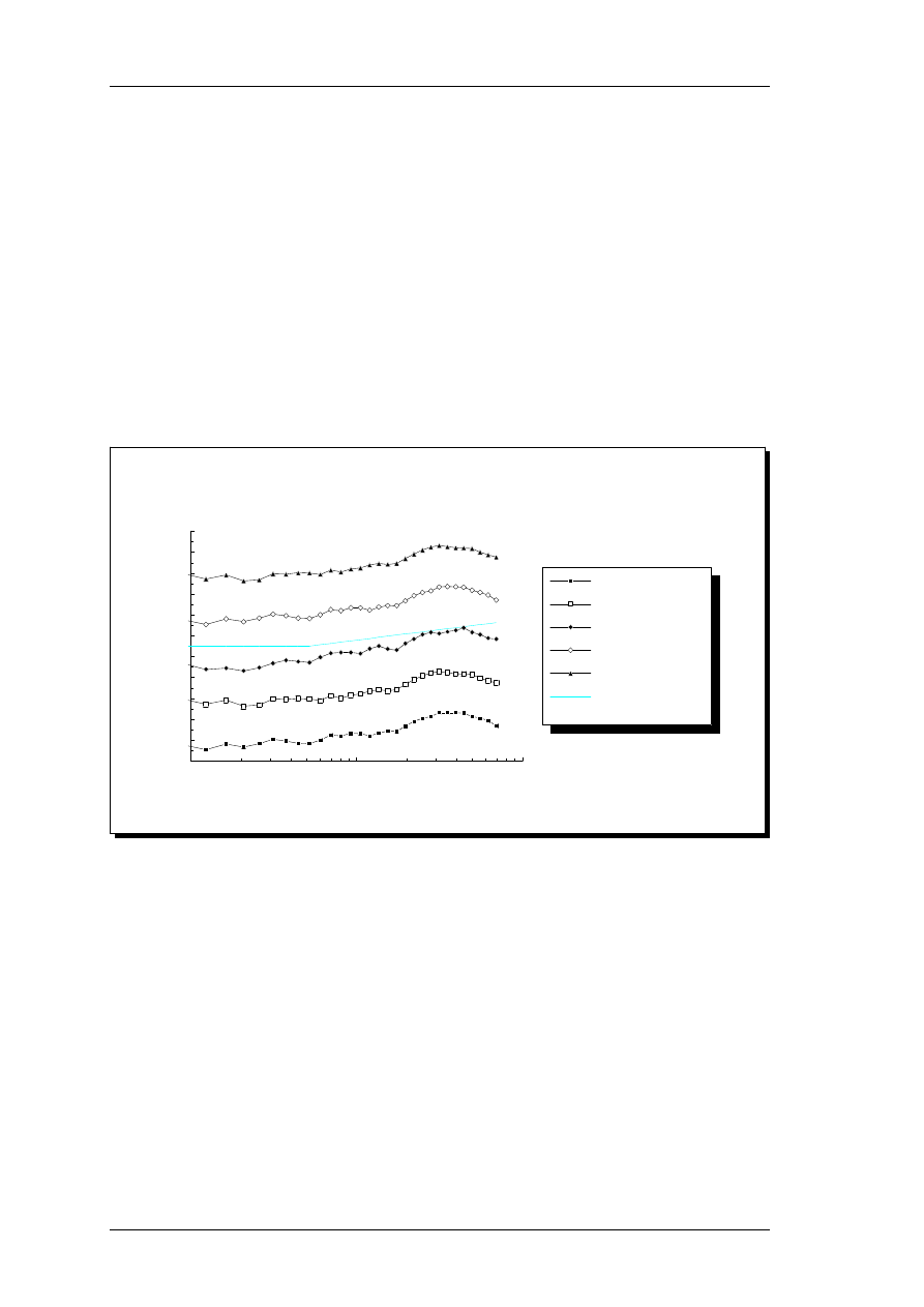
4.2.2 Noise signals.
For a white noise masking signal, the classical masked pure tone threshold (Zwicker &
Fastl, 1990, Fig. 4.1) follows a horizontal line up to approximately 500 Hz, followed by
a sloping line at +10 dB per decade (+3 dB/octave).
For white noise at varying levels, the auditory model excitation patterns are shown in
figure 14. Also shown is the masked threshold for a white noise signal at 30 dB SPL/Hz,
approximated by a two-segment line (from Zwicker & Fastl (1990), fig. 4.1).
Excitation patterns, white noise
f, kHz
Le, dB
-10
0
10
20
30
40
50
60
70
80
90
100
0.1
1
10
-10 dB SPL/Hz
10 dB SPL/Hz
30 dB SPL/Hz
50 dB SPL/Hz
70 dB SPL/Hz
30 dB SPL/Hz
(Zwicker & Fastl, 1990)
14.
Excitation patterns for a white noise signal at various levels, compared to an idealized model of
masked threshold for a 30 dB SPL/Hz white noise signal.
There is a considerable difference between the model output and the masked thresholds,
at low frequencies (~ -10 dB). The bandwidth of the ERB-filters continues to decrease
below 500 Hz, whereas the classical critical-band scale has constant bandwidth (= 100
Hz) below 500 Hz (Moore & Glasberg, 1987). Therefore, the excitation pattern
continues to drop below this frequency. The model output curve is also irregular
compared to the masking curves from Zwicker & Fastl (1990) - probably due to a
smoothing of their data.
Page 56
An auditory model with hearing loss.
4. Verification
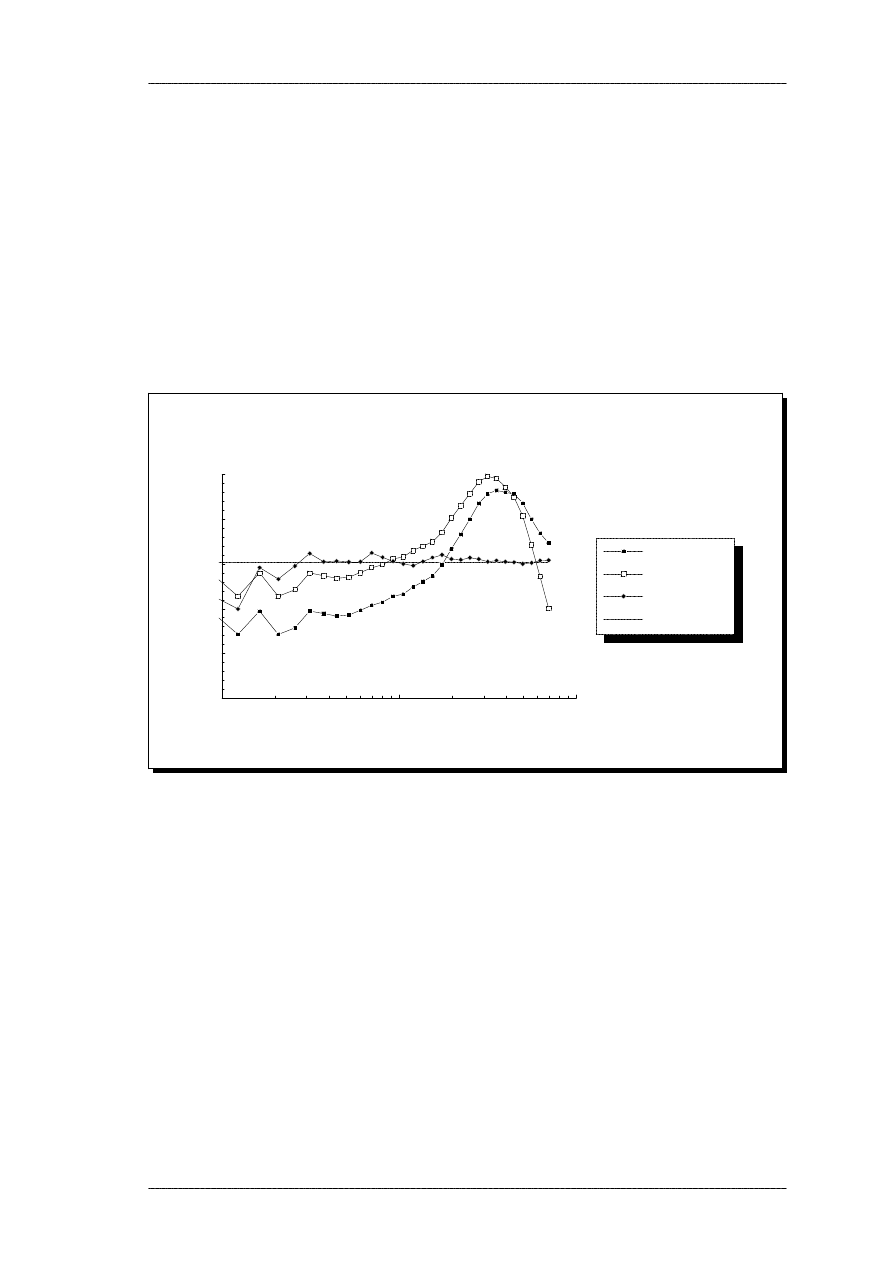
Another relevant noise signal in psychoacoustic testing is the so-called uniform exciting
noise (UEN), ie. noise that causes the same excitation in all channels. The spectrum of
such a signal has been proposed by Zwicker & Feldtkeller (1967). Their noise signal was
tested in the auditory model along with a white noise signal (see Figure 15). The
purpose of UEN is to measure psychoacoustic parameters, without misleading results
due to the spread of excitation, for instance to measure the loudness growth function in
one auditory filter channel (specific loudness - see section 3.5.1).
Excitation patterns, 80 dB SPL
f, kHz
Le, dB
50
55
60
65
70
75
0.1
1
10
White noise
UEN (Z&F, 1990)
Modified UEN
Ideal
15.
Excitation patterns for white noise, uniform exciting noise (Zwicker & Fastl, 1990) and modified
uniform exciting noise, all at 80 dB SPL. Also shown is the ideal excitation, when the signal
power is evenly distributed across channels.
The original UEN does not account for the ear-canal response around 3 kHz, as seen
from the excitation pattern.
For the purpose of further testing of the specific loudness growth function (section 4.3.1,
Figure 21), a modified UEN was then created as follows: The excitation pattern for a 80
dB SPL white noise signal (40 dB SPL/Hz) was obtained, and a 256-tap digital filter
with the inverse amplitude response was then designed by means of the FILTSPEC
program (ODIN, 1988). By convolving the white noise signal with the digital filter, the
modified UEN was obtained. At low frequencies (< 300 Hz), the FFT-analysis framesize
An auditory model with hearing loss.
Page 57
4. Verification

in the auditory model and the length of the digital filter were both too short to control
and measure the frequency response properly, as seen in the graph.
4.2.3 Impaired frequency selectivity.
Frequency selectivity in hearing impaired listeners has been the subject of several studies
- Florentine et al (1980), Ludvigsen (1985) and Dubno & Schafer (1992), to name a few.
For comparison with the auditory model, the recent results of Dubno & Schafer (1992)
have been chosen, due to a straightforward stimulus choice and results that were easily
obtained from the graphs in the paper. The subjects were six individuals with
mild-to-moderate sensorineural hearing losses, four with typical sloping, high-frequency
losses and two with flat hearing loss. Masked pure-tone thresholds were obtained with
narrow-band 200 Hz noise bands, centered at 1200 Hz. The test-tone frequencies were
0.63, 0.80, 1.00, 1.20, 1.25, 1.40, 1.60, 2.00, 2.50, 3.15, and 4.00 kHz, and all signals
were presented via a TDH-49 headphone. All threshold values are provided in dB SPL,
presumably recorded on a 6 cm
3
(IEC303) coupler.
For the model simulations, the four subjects with sloping losses were averaged to one
group, ie. absolute thresholds were averaged and masked thresholds were averaged.
Same procedure was used for the two subjects with flat losses. The 200 Hz NB-noise
signals in the experiment was slightly wider than a normal critical band centered at 1200
Hz (190 Hz, Zwicker & Fastl (1990)) and wider than one ERB-band (155 Hz, Glasberg
& Moore (1990)). It was presented at two spectrum levels, 40 dB SPL/Hz and 60 dB
SPL/Hz. For the present auditory modeling, a 1200 Hz pure-tone signal with the same
sound pressure level was used for simplicity (63 dB SPL and 83 dB SPL), which can be
justified because of the absence of beats (difference tones) in the model.
The results for the 40 dB SPL/Hz masker are shown, only for the sloping loss group, in
Figure 16.
Page 58
An auditory model with hearing loss.
4. Verification
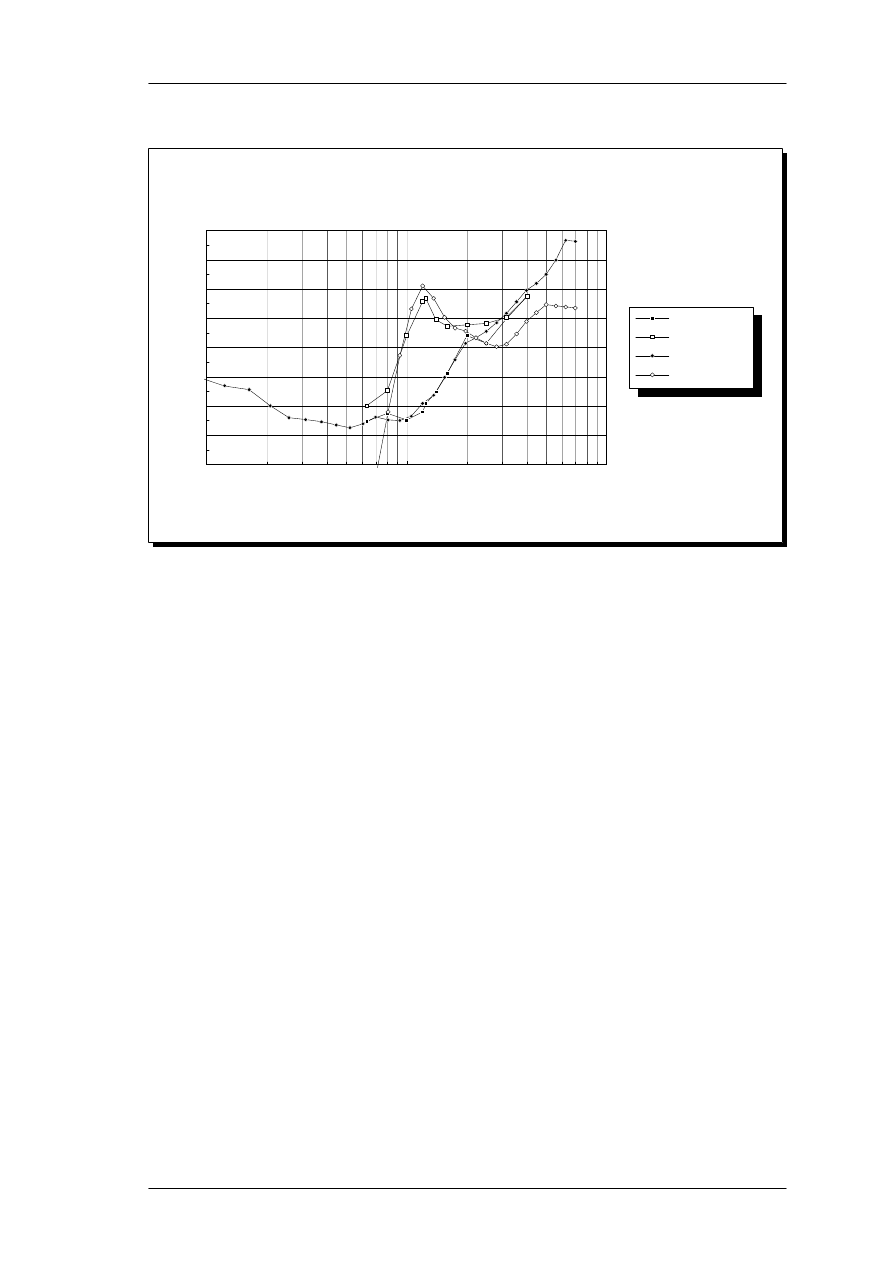
Impaired narrow-band masking
Sloping loss
f, kHz
Le, dB ; Lt, dB SPL
0
10
20
30
40
50
60
70
80
0.10
1.00
10.00
Avg thr.
Avg. masked thr.
Model thr. exc.
Model masked exc.
40 dB SPL/Hz NB noise = 63 dB SPL tone
16.
Average masked and absolute thresholds for four subjects with sloping loss (Lt, in dB SPL),
compared to the excitation in the auditory model (Le, dB). The masker was a 1200 Hz, 200
Hz-wide noise band at 40 dB SPL/Hz, and the model stimulus was a 1200 Hz pure tone at 63 dB
SPL.
The model excitation pattern for the threshold matches the absolute thresholds in the
range were they were obtained (630 Hz - 4 kHz). Outside this range, thresholds were
extrapolated to normal hearing at low frequency and increasing loss at high frequencies.
The close match was expected, since the model parameter file contained the audiometric
thresholds, expressed in dB HL.
In the masked situation, there is a good agreement between the experimental data and
the model output. The upward spread of masking is reproduced by the model, with
some deviation close to the absolute threshold. The model excitation pattern does not
approach the absolute threshold asymptotically, but simply intersects it. This deviation
could be alleviated if the threshold parameter, r, was included in the roex filter shape
(equation 2, section 3.4), instead of using threshold in the loudness function only.
For the 60 dB SPL/Hz masker and the sloping loss group, the results are shown in
Figure 17.
An auditory model with hearing loss.
Page 59
4. Verification
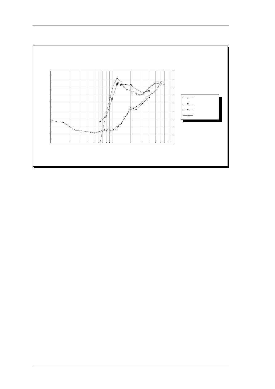
Impaired narrow-band masking
Sloping loss
f, kHz
Le, dB ; Lt, dB SPL
0
10
20
30
40
50
60
70
80
90
0.10
1.00
10.00
Avg thr.
Avg. masked thr.
Model thr. exc.
Model masked exc.
60 dB SPL/Hz NB noise = 83 dB SPL tone
17.
Average masked and absolute thresholds for four subjects with sloping loss (Lt, in dB SPL),
compared to the excitation in the auditory model (Le, dB). The masker was a 1200 Hz, 200
Hz-wide noise band at 60 dB SPL/Hz, and the model stimulus was a 1200 Hz pure tone at 83 dB
SPL.
The masked thresholds indicate a larger amount of upward spread of masking than the
model, but there is a reasonable agreement. The model excitation pattern bends upward
again above 3 kHz and runs parallel to the threshold excitation, due to almost complete
loss of frequency selectivity for the large losses present at higher frequencies. Thus, the
high-frequency filters are able to "see" the stimulus at 1200 Hz. This high-frequency
excitation may be overestimated, but no firm conclusion can be made, since the hearing
losses above 4 kHz were extrapolated for the simulations.
The same overestimated upward spread of masking is evident for the two subjects with
moderate, flat losses as shown in figure 18.
Page 60
An auditory model with hearing loss.
4. Verification
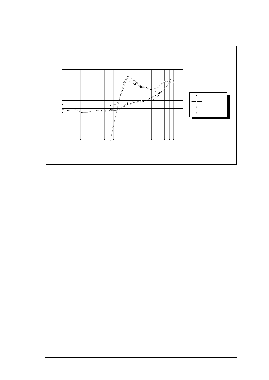
Impaired narrow-band masking
model vs. experimental data.
f, kHz
Le, dB ; Lt, dB SPL
0
10
20
30
40
50
60
70
80
90
0.10
1.00
10.00
Avg thr.
Avg. masked thr.
Model thr. exc.
Model masked exc.
60 dB SPL/Hz NB noise = 83 dB SPL tone
18.
Average masked and absolute thresholds for two subjects with flat loss (Lt, in dB SPL), compared
to the excitation in the auditory model (Le, dB). The masker was a 1200 Hz, 200 Hz-wide noise
band at 60 dB SPL/Hz, and the model stimulus was a 1200 Hz pure tone at 83 dB SPL.
Except for this discrepancy and an elevated masked threshold at 630 Hz relative to the
model, there is good agreement between the two curves.
Based on these three cases, the model appears to represent the reduced frequency
selectivity in mildly-to-moderately hearing-impaired listeners well on the average. There
may be large individual differences (Tyler, 1986), that a general model cannot represent,
unless frequency selectivity is measured on an individual basis.
4.3
Loudness.
4.3.1 Loudness growth in normal and impaired hearing.
The loudness function in the model was first compared to loudness growth functions for
normal hearing. The stimulus used for this was pure tones at octave frequencies. The
signal files contained 26 frames, with a stepwise increase of 2 dB between frames, thus
An auditory model with hearing loss.
Page 61
4. Verification
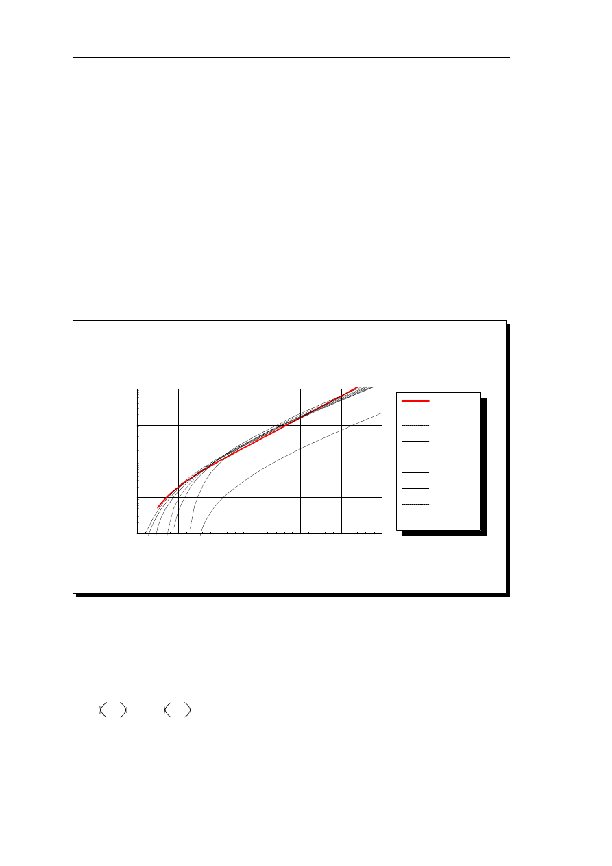
covering a 50 dB dynamic range. If necessary, two overlapping 50 dB ranges were used
(by changing the auditory model parameter file), to cover the entire dynamic range.
Data on binaural loudness in sones was obtained from Scharf (1978b). For 1 kHz, the
loudness as function of dB SPL is listed in a table, whereas the loudness growth
functions for other frequencies are derived from the ISO 226 (1987) equal loudness
contours, that originate from Robinson and Dadson (1956).
The loudness growth functions for the auditory model are shown in Figure 19 along with
the 1 kHz loudness growth function from Scharf (1978b).
Loudness growth
Binaural
dB SPL, free field
Sones
0.01
0.10
1.00
10.00
100.00
0
20
40
60
80
100
120
1 kHz
Scharf (1978)
125 Hz
250 Hz
500 Hz
1000 Hz
2000 Hz
4000 Hz
8000 Hz
19.
Binaural loudness growth
functions
for various frequencies. The 1 kHz loudness
function can be compared to actual loudness data from Scharf (1978b).
The actual loudness curve from Scharf follows the power law above 40 dB SPL:
N
=
k
P
P
0
0.6
=
k
I
I
0
0.3
(23)
which is a straight line in a dB - log sones plot. k is chosen to obtain 1 son at 40 dB
SPL. According to Scharf (1978b), all the loudness curves should coincide with this line
Page 62
An auditory model with hearing loss.
4. Verification

at high levels, except the 8 kHz curve, which is shifted down, due to a larger
transmission factor (e.g. attenuation) at this frequency. At low frequencies, we see
elevated thresholds and thus more rapid growth of loudness near the threshold.
The 1 kHz model curve drops down towards thresholds at a slightly higher level, and the
curve is shifted roughly 4 dB at 0.05 sones, an acceptable deviation. At higher levels
(40-80 dB SPL), there is a slight overshoot compared to the power law line for all
frequencies. Since the model uses a different filter shape and a higher number of critical
bands (30 in the range 87 Hz - 7 kHz vs. Zwicker's 21 in the same frequency range), the
total loudness may be higher, when no adjustment of N
0
' has been made. Without any
precise, quantitative description of loudness, there is no obvious reason to make a
modification.
At higher levels (~80 dB SPL), the loudness curve drops below the power law line, in
particular for the higher frequencies. This is probably due to the upper frequency limit
(10 kHz) that was used in the current simulations, which limits the upward spread of
masking, cutting off the high-frequency tail of the excitation pattern and resulting in an
incorrectly low loudness. These excitation patterns are shown in Figure 12. Future
simulations with higher bandwidth (ie. higher sample rate) might confirm this.
When hearing loss is introduced, the model should exhibit 'recruitment', ie. abnormally
steep growth of loudness. For a series of flat hearing losses, the 1 kHz loudness growth
function was evaluated as shown in figure 20.
2
An auditory model with hearing loss.
Page 63
4. Verification
2
The curves were obtained for a 1060 Hz pure tone, since this frequency is
centered in a filter channel of the model.
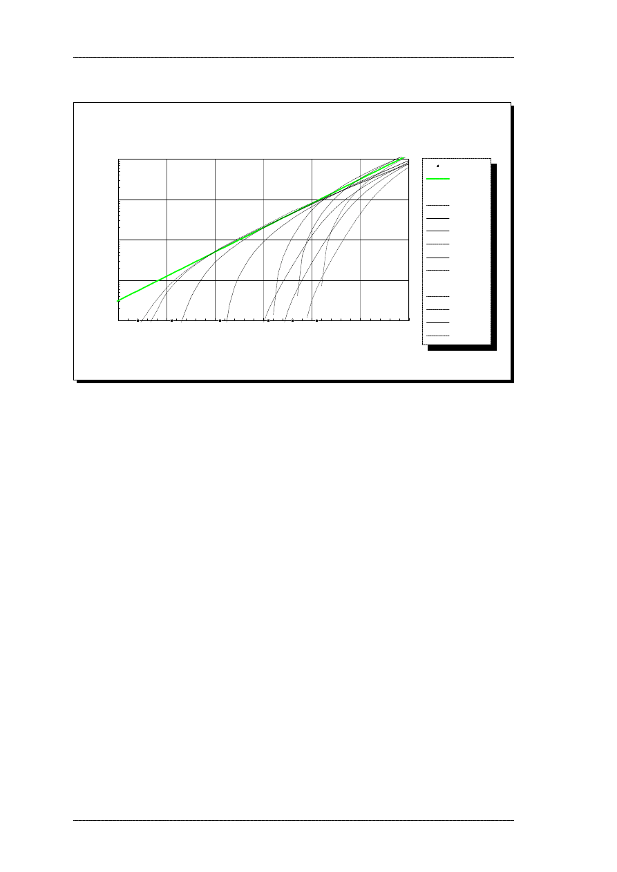
Loudness growth
1 kHz, Monaural
dB SPL, free field
Sones
0.01
0.1
1
10
100
0
20
40
60
80
100
120
MAF
Power law
Model:
0 dB HL
15 dB HL
35 dB HL
55 dB HL
65 dB HL
75 dB HL
H&M data fit:
0 dB HL
55 dB HL
65 dB HL
75 dB HL
20.
Loudness growth as a function of level and hearing loss. The heavy line represent
the 0.3 exponent power law and the markers along the abscissa indicate the
monaural free-field threshold. Also shown are the fitted loudness growth functions
to experimental data by Hellman and Meiselman (1990).
In the figure, the free-field thresholds are indicated with filled squares along the abscissa.
In a log sones plot, the loudness function should approach these levels asymptotically,
since per definition loudness is N = 0 at threshold. This is clearly the case for high
thresholds, whereas the 0 and 15 dB HL losses have more shallow slopes close to
threshold. The recruitment effect is very obvious, since all loudness functions approach
the power law line at high levels (> 100 dB SPL). A modification of the loudness growth
exponent at high levels as proposed by Leijon and discussed previously (section 3.5), is
thus not needed For small threshold values, there is a slight underestimation of loudness
for high levels, due to the aforementioned band limiting of upward spread of masking.
For high threshold values, there is a slight overestimation, which is due to the increased
spread of masking, ie. almost no frequency selectivity.
Hellman & Meiselman (1990) presented data on loudness growth functions for
hearing-impaired listeners with noise-induced losses of 55, 65 and 75 dB HL. No
detailed statistics on the audiogram shape was presented. The fitted loudness functions
Page 64
An auditory model with hearing loss.
4. Verification

(obtained from the paper) were scaled by means of a spreadsheet program to coincide
with the power law at high levels (*1.85) and plotted in Figure 20. Their loudness model
for impaired hearing is based on a loudness summation model by Zwislocki (1965).
There is a large discrepancy between these data and the model output, ie. the model
loudness functions rise more steeply than the fitted lines presented by Hellman &
Meiselman (1990). The fitted lines indicate linear growth of loudness near threshold,
with the 0.01 sones levels being below threshold, however these lines extend below the
lowest loudness value in the actual data (0.4 sones). The large difference between the
two models has implications on the degree of recruitment present for a given hearing
loss. The Zwislocki loudness model should be subject to more investigation and possibly
be implemented in the model in the future.
The correct shape of the specific loudness function is tested by using 'uniform exciting
noise' (Zwicker & Fastl, 1990), ie. a noise signal, shaped such that the resulting
excitation pattern is flat. The reason for this is that a for a flat excitation pattern, an
upward spread of masking will have little or no effect, since there is energy present in all
bands. The preparation of such a signal was presented in section 4.2.2. The noise signal
was multiplied by a 2 dB step staircase, such that the signal level increased 2 dB per each
8 frames over a 50 dB range. For none or little hearing loss, two overlapping 50 dB
ranges were used to cover the entire dynamic range. By averaging 8 power spectra prior
to the loudness calculation the result was fairly stable. The obtained loudness curves are
still not perfectly smooth as shown in figure 21. The hearing losses simulated in the
model were flat, e.g. constant dB HL across the audiometric frequencies.
An auditory model with hearing loss.
Page 65
4. Verification
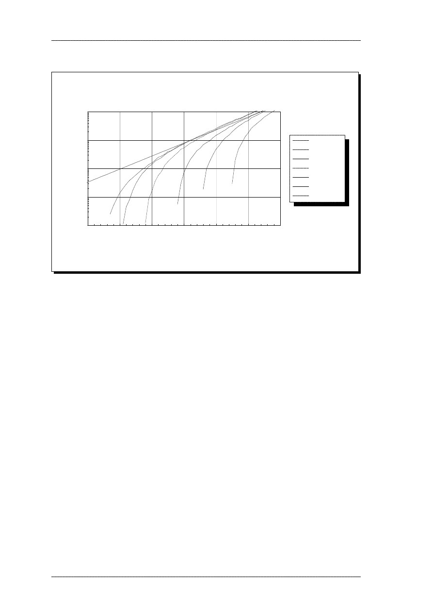
Loudness growth
UEN, Monaural
dB SPL, free field
Sones
0.01
0.10
1.00
10.00
100.00
0
20
40
60
80
100
120
Power law (0.23)
Zwicker & Fastl
0 dB HL
15 dB HL
35 dB HL
55 dB HL
75 dB HL
21.
Monaural loudness growth function for uniform exciting noise with various flat
hearing losses. Also shown are the power law line for the specific loudness growth
function and the measured loudness function near threshold (Zwicker & Fastl,
1990) .
The model loudness curves were compared to results from Zwicker and Fastl (1990).
Their original data on binaural loudness were converted to monaural values by halving
the loudness, as discussed in section 3.5.1. At high levels, the model output curves agree
reasonably well, when there is a small or no hearing loss. The actual threshold of the
model for 0 dB hearing loss is elevated by roughly 10 dB in comparison with Zwicker &
Fastl's binaural results, with at least 3 dB due to the missing binaural-to-monaural
threshold correction. Even when the model thresholds are approximately correct for
pure tone stimuli, it is difficult to predict the absolute threshold of the noise signal, since
the detection factor (s in eqn. 16) most likely will be different when broad-band noise
signals are detected in the presence of the internal background noise. No further changes
were made to the model to correct this threshold deviation.
Page 66
An auditory model with hearing loss.
4. Verification
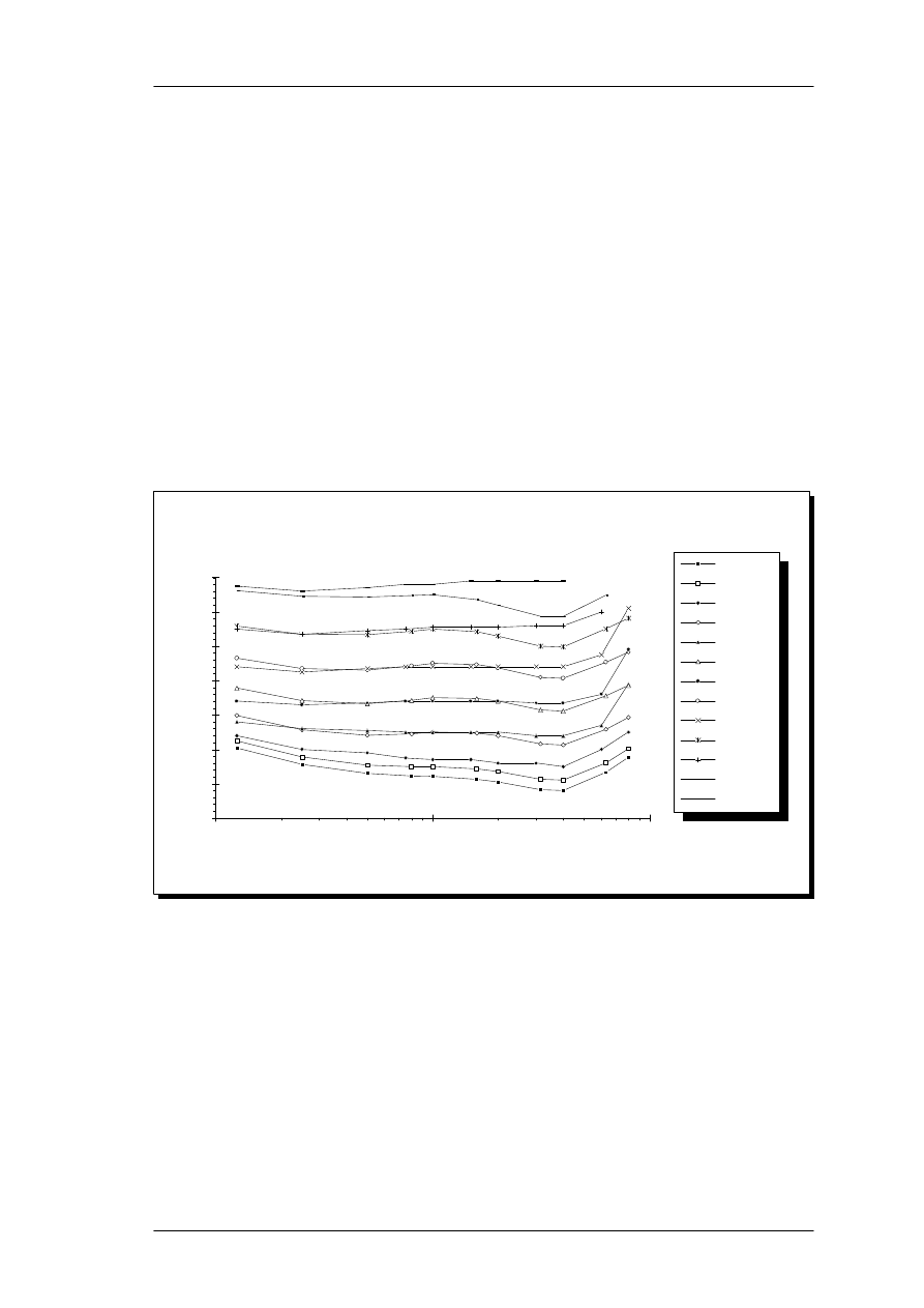
4.3.2 Equal loudness level contours.
Based on the loudness growth curves from section 4.3.1, equal loudness level contours
can be constructed, ie. the level of a pure tone at a given frequency at which the level is
equally loud as a 1 kHz tone. Thus, the 20 phon curve is the contour curve indicating
the level that a pure tone should have to be perceived as loud as a 20 dB SPL, 1 kHz
tone. Since the model output is in sones, the sone value corresponding to each 10 phon
increase can be found from the 1 kHz loudness growth curve by Scharf (1978b), shown
in Figure 19. The equal loudness curves derived in this way from the auditory model
output are shown in figure 22.
Equal loudness level contours
Binaural, Normal hearing
Frequency, Hz
dB SPL, free field
-20
0
20
40
60
80
100
120
100
1000
10000
4 phon (THR)
10 phon
10 phonM
30 phon
30 phonM
50 phon
50 phonM
70 phon
70 phonM
90 phon
90 phonM
110 phon
110 phonM
22.
Equal loudness contours derived from model loudness growth functions (indicated as phonM
curves) and reference equal loudness curves from ISO226 (indicated as phon curves). The 4 phon
curve is the absolute threshold, also termed minimum audible field (MAF).
The contours derived from the auditory model can be compared to the standard equal
loudness level contours published in ISO226. The lowest curve (10 phonM) is elevated,
but parallel to the ISO226 curve. This confirms that the effective thresholds in the model
are a little to high (figure 20 for 1 kHz). The loudness function initialization procedure
used in the model (section 3.5.1) will force the shape of the phon curve to the correct
value near threshold. At higher levels (30-50-70 phon), the two sets of curves deviate at
An auditory model with hearing loss.
Page 67
4. Verification

3-4 kHz, ie. the model fails to reproduce the dip in the curves. This could be corrected
by using the 100 phon ELC correction curve (flat below 1 kHz) shown in Figure 2,
causing the dip to be roughly 5 dB deeper. At higher levels, this difference becomes
more pronounced, along with a larger difference at 6 kHz - these differences are
equivalent of loudness curves dropping below the power law line as shown in Figure 19.
This is due to the upper frequency limit in this configuration of the model that imposes
an artificial constraint on the upward spread of masking for high-level, high-frequency
signals, as discussed in section 4.2.1. Above threshold, the 8 kHz values are very
different, since this frequency is above the highest channel in the present model
configuration (7 kHz).
4.4
Temporal resolution.
Since temporal resolution has not been included in the model specifically, the temporal
properties have not been evaluated. When the input signal is analyzed in overlapping
frames, the model excitation will obviously fade out, as a signal is turned off, thus
emulating some kind of post-masking. This will also prevent the model from detecting
gaps in the signal, when below a given size. However, a quantification of these
properties was not considered meaningful and thus not pursued.
Page 68
An auditory model with hearing loss.
4. Verification
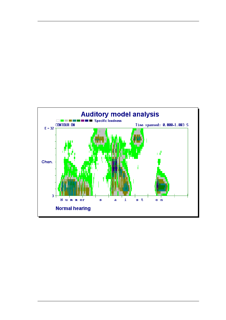
5.1
Perception of speech sounds.
The obvious advantage of a signal processing structure implemented as a program, as
opposed to a mathematical formulation of masking patterns, loudness growth functions
etc., is that it can be used to analyze complex patterns and real-world signals. One
example of such an application is shown in Figure 23.
23.
The danish utterance "Nummer saisten" (Number sixteen) processed through the auditory model
with normal hearing and viewed as a grey-scale mapping of specific loudness. The signal level
was set at 65 dB SPL. The x-axis is time and the y-axis is channel number in the model.
The 1-second utterance "Nummer saisten" ("Number sixteen") was processed through
the auditory model with 33 channels spaced between E = 3 and 32. The signal was
processed in 256-point frames with a 75% overlap. The long-term level L
eq
was set to
65 dB SPL in free field. The grey-scale in the plot is set such that black equals maximum
specific loudness and each step represents fixed decrease in specific loudness (ie. a linear
scale). Due to the power law used for loudness encoding as opposed to the
5
Processing of real-world signals.
An auditory model with hearing loss.
Page 69
5. Processing of real-world signals
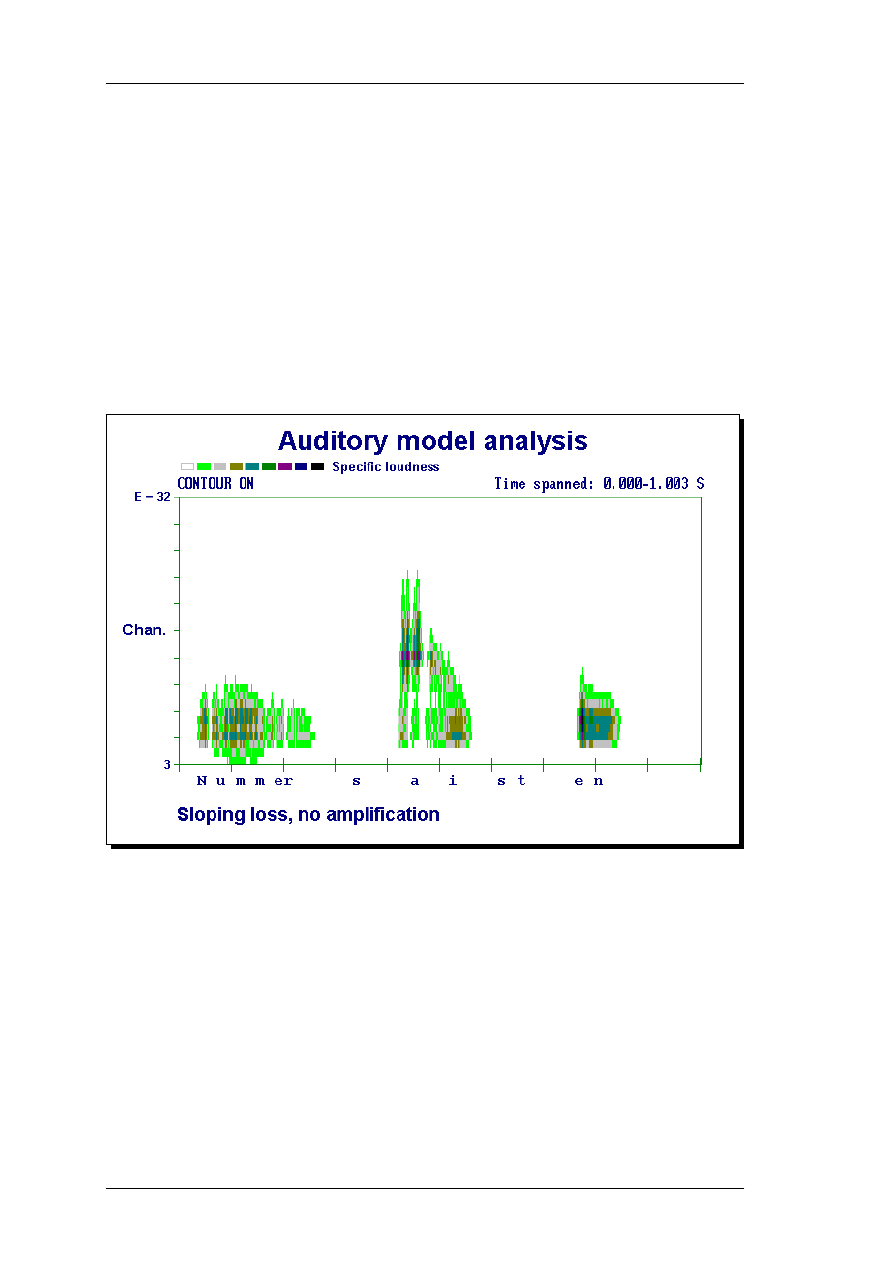
log-transformation typically used for excitation patterns, the loudness 'spectrogram' will
cover a smaller dynamic range. It is possible to distinguish formant patterns for the
vowels, and the general pattern is quite detailed.
The model was then used with a typical sensorineural sloping loss, the average loss from
a previous experiment (Nielsen, 1992) was entered. When processing the same utterance
without any amplification, the specific loudness 'spectrogram' contains less information
as shown in Figure 24.
24.
The danish utterance "Nummer saisten" (Number sixteen) processed through the auditory model
with a typical sensorineural, sloping hearing loss, and viewed as a grey-scale mapping of specific
loudness. The signal level was set at 65 dB SPL, and no amplification was applied. The x-axis is
time and the y-axis is channel number in the model.
Only the low-frequency segments of the signal are visible and the vowel 'a' has less
high-frequency information. The next step was to apply a linear amplification to the
speech signal, using the POGO II amplification rule (Schwartz et al, 1988) to specify the
insertion gain. A 64-tap filter was designed and the signal was convolved with this filter.
Page 70
An auditory model with hearing loss.
5. Processing of real-world signals
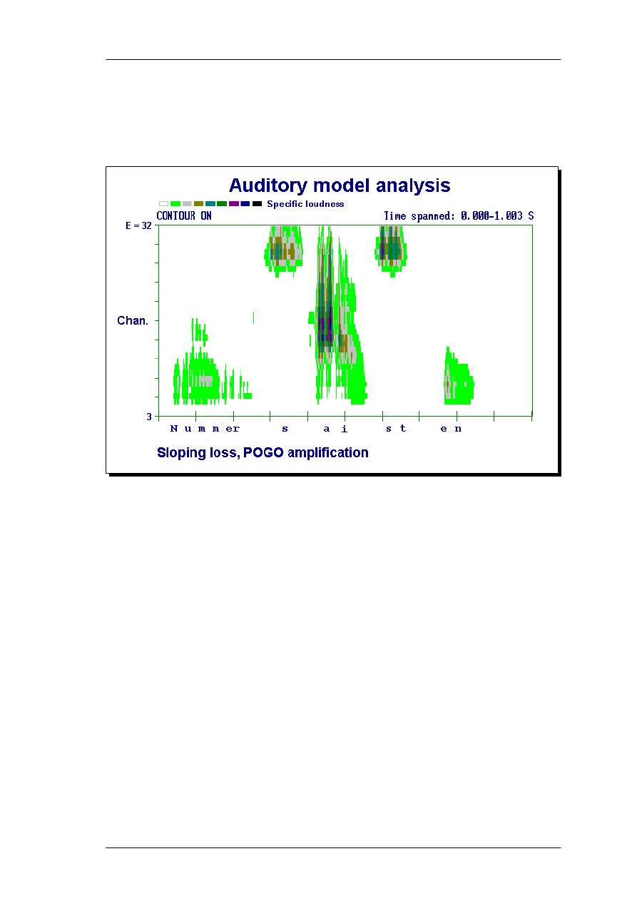
The auditory model parameter file used scaling equivalent of an L
eq
of 65 dB SPL prior
to amplification. The result is shown in Figure 25.
25.
The danish utterance "Nummer saisten" (Number sixteen) processed through the auditory model
with a typical sensorineural, sloping hearing loss, and viewed as a grey-scale mapping of specific
loudness. The signal level was set at 65 dB SPL, and amplification was applied according to the
POGO rule. The x-axis is time and the y-axis is channel number in the model.
The amplification ensures more loudness and audibility for loud sounds, but the weak
sounds are not visible. Furthermore, the increased upward spread of masking causes the
audible sounds to be spread across more channels as seen for the vowel 'a'.
5.2
Performance and future improvements.
The above examples show how the model is useful for a visualization of
hearing-impaired perception of complex sounds, and thus for a qualitative analysis of
hearing-aid processed signals. For a quantitative analysis, the current graphing program
An auditory model with hearing loss.
Page 71
5. Processing of real-world signals

(imported into HyperSignal Workstation) is not adequate, and future versions of the
model should rather include dedicated graphing functions.
The model performs the processing of this 1-second signal in 111 seconds on a 486/25
MHz PC, using 256-point signal frames that were overlapped 75%. It is thus useful for
immediate analysis of short signals. For longer signals, several signals could for instance
be processed overnight in a batch-file.
Page 72
An auditory model with hearing loss.
5. Processing of real-world signals

An auditory model based on psychoacoustic theory has been presented. The advantage
of this approach, rather than using a physiological model, was discussed. The model has
been specified, developed and implemented based on selected results from the literature.
As an attempt to unify various psychoacoustic models for filter shapes, loudness growth
etc., the model represents a compromise that can be subject to controversies.
The elements of the model are: Power spectrum calculation, equalizations and coupler
corrections, an auditory filter bank with or without hearing loss, and loudness growth
functions for normal and impaired hearing. The temporal properties of the normal and
impaired hearing system have not been included in the current implementation, due to
time limitations in the project.
The model was verified against various results from the psychoacoustic literature. For
normal hearing, the model reproduced masking patterns for narrow-band noise well,
underestimating upward spread of masking at high masker levels. For hearing-impaired
subjects, the upward spread of masking was furthermore limited by the upper frequency
limit used for the simulations. Nevertheless, the model correctly reproduced
narrow-band masked thresholds well for a small, selected group of impaired subjects.
The loudness growth function was generally correct, but loudness was underestimated at
high levels, compared to the usual 0.3 power law used at high levels. This discrepancy
was also due to the frequency limit in the model. As a consequence, the equal loudness
level contours for normal hearing were also incorrect at high levels. For impaired
hearing, the model also produced the proper loudness growth according to Zwicker &
Fastl (1990), but in disagreement with an alternative loudness model used by Hellman &
Meiselman (1990).
Based on the above simulations and verifications of the model, it can be justified, that the
model represents known psychoacoustic properties of the normal and impaired human
ear, with the exception of temporal properties.
6
Conclusion.
An auditory model with hearing loss.
Page 73
6. Conclusion

As an example of a real-world application of the model, loudness spectrograms for a
speech utterance were presented. By introducing hearing loss, the speech sounds
became less audible and less detailed, a problem that linear amplification did not solve
properly. This demonstrated how the model could be used for hearing aid development
and evaluation.
Future improvements of the model include: Models of temporal processing for normal
hearing and hearing impairment. Also graphical output and a more user-friendly
interface might be added.
Page 74
An auditory model with hearing loss.
6. Conclusion

Agerkvist, F.A. (1992). Time-frequency analysis with temporal and spectral resolution
as the human auditory system. Proc. IEEE-SP Int. Symp. on Time-Frequency and
Time-Scale analysis. Vancouver, BC, Canada, 1992.
Allen, J.B. (1985). Cochlear modeling. IEEE ASSP Magazine, January 1985.
Allen, J.B. (1990). Modeling the noise damaged cochlea. In: The Mechanics and
Biophysics of Hearing. (ed. Dallos, Geisler, Matthews, Ruggero & Steele), Springer,
Berlin, 1990.
Allen, J.B, Hall, J.L. and Jeng, P.S. (1990). Loudness growth in 1/2 octave bands
(LGOB) - A procedure for the assessment of loudness. J Acoust Soc Am, 88(2), 745 -
753.
Barfod, J. (1976). Multichannel compression hearing aids. Report no. 11, The
Acoustics Laboratory, Technical University of Denmark.
Berger, E.H. (1981). Re-examination of the low-frequency (50 - 1000 Hz) normal
thresholds of hearing in free and diffuse sound fields. J Acoust Soc Am, 70(6), 1635 -
1645.
Bentler, R.A. and Pavlovic, C.V. (1989). Transfer functions and Correction Factors
Used in Hearing Aid Evaluation and Research. Ear Hear, 10(1), 58 - 63.
Bentler, R.A. and Pavlovic, C.V. (1992). Addendum to "Transfer functions and
Correction Factors Used in Hearing Aid Evaluation and Research". Ear Hear, 13(4),
284 - 286.
Buus, S. (1992). Experiments with an auditory model and auditory filter spacing.
Personal communication.
Buus, S. & Florentine, M.(1992). Recent results on free-field monaural thresholds.
Personal communication.
Cohen, J (1989). Application of an auditory model to speech recognition. J Acoust Soc
Am, 85(6), 2623 - 2629.
de Boer, E. (1985). Auditory Time Constants: A paradox? In: Time Resolution in
Auditory Systems. (ed. Michelsen). Springer, Berlin, 1985
Dubno, J.R. & Schafer, A.B. (1992). Comparison of frequency selectivity and
consonant recognition among hearing-impaired and masked normal-hearing listeners. J
Acoust Soc Am, 91(4), 2110 - 2121.
7
References.
An auditory model with hearing loss.
Page 75
7. References

Evans, E.F. (1975a). Cochlear nerve and cochlear nucleus. Chapter 1 in: Handbook of
sensory physiology, vol. V/2: Auditory system. (ed: Keidel, W.D. and Neff, W.D).
Springer-Verlag, New York, pp. 1 - 96.
Evans, E.F. (1975b). The sharpening of cochlear frequency selectivity in the normal and
abnormal cochlea. Audiology 14, 419 - 442.
Evans, E.F. (1985). Aspects of the neural coding of time in the mammalian peripheral
auditory system relevant to temporal resolution. in: A Michelsen (ed.). Time resolution
in auditory systems. Springer, Berlin, pp. 74 -95.
Evans, E.F. and Elberling, C. (1982). Location-Specific Components of the Gross
Cochlear Action Potential. Audiology 21, 204 - 227.
Fink, F. (1989). Introduktion til auditiv modellering (Danish). Publ. R 89-8, Institute of
Electronics Systems, Aalborg University Center.
Florentine, M., Buus, S., Scharf, B. and Zwicker, E. (1980). Frequency selectivity in
normally-hearing and hearing-impaired observers. J Speech Hear Res 23, 646 - 669.
Florentine, M. and Zwicker, E. (1979). A model of loudness summation applied to
noise-induced hearing loss. Hear Res 1, 121 - 132.
Glasberg, B.R. and Moore, B.C.J. (1986). Auditory filter shapes in subjects with
unilateral and bilateral cochlear impairments. J Acoust Soc Am, 79(4), 1020 - 1033.
Glasberg, B.R. and Moore, B.C.J. (1990). Derivation of auditory filter shapes from
notched-noise data. Hear Res 47, 103 - 138.
Harrison, R.V. and Evans, E.F. (1982). Reverse correlation study of cochlear filtering in
normal and pathological guinea pig ears. Hear Res 6, 303 - 314.
Hellman, R.P. and Meiselman, C.H. (1990). Loudness relations for individuals and
groups in normal and impaired hearing. J Acoust Soc Am, 88(6), 2596 - 2606.
Hermansky, H. (1990). Perceptual linear predictive (PLP) analysis of speech. J Acoust
Soc Am, 87(4), 1738 - 1752.
Hirahara, T. and Komakine, T. (1989). A computational cochlear nonlinear
preprocessing model with adaptive Q circuits. Proc ICASSP 1989, 496 - 499.
Humes, L.E., Espinoza-Varas, B., and Watson, C.S. (1988). Modeling sensorineural
hearing loss. I. Model and retrospective evaluation. J Acoust Soc Am, 83(1), 188 -202.
Humes, L.E. and Jesteadt, W. (1991). Models of the effects of threshold on loudness
growth and summation. J Acoust Soc Am, 90(4), 1933 -1943.
Page 76
An auditory model with hearing loss.
7. References

IEC 303 (1970). IEC provisional reference coupler for the calibration of earphones used
in audiometry. 1. edition.
IEC 318 (1970). An IEC artificial ear, of the wideband type, for the calibration of
earphones used in audiometry. 1. edition.
IEC 711 (1981). Occluded-ear simulator for the measurement of earphones coupled to
the ear by ear inserts. 1. edition.
ISO 226 (1987). Acoustics - Normal equal-loudness level contours.
ISO/TC43/WG1/N160 (1991). Second Working Draft for a revision of ISO 226
(October 1991).
ISO 389 (1991). Acoustics - Standard reference zero for the calibration of pure tone air
conduction audiometers.
Karjalainen, M. (1985). A new auditory model for the evaluation of sound quality of
audio systems. Proc ICASSP 1985, Tampa.
Karjalainen, M. (1987). Auditory models for speech processing. Proc. Int. Congr. Phon.
Sciences. Tallinn.
Kates, J.M. (1991). A time-domain digital cochlear model. IEEE Trans Sig Proc ,
39(12), 2573 - 2592.
Killion, M.C. (1978). Revised estimate of minimum audible pressure: Where is the
"missing 6 dB"? J Acoust Soc Am, 63(5), 1501 - 1508.
Killion, M.C. (1984). New insert earphones for audiometry. Hearing Instruments, 35,
45 - 46.
Leijon, A. (1989). Optimization of hearing-aid gain and frequency response for cochlear
hearing losses (Ph.D. thesis). Technical report no. 189. Chalmers University of
Technology, Göteborg, Sweden.
Liberman, M.C. and Dodds, L.W. (1984). Single-neuron labeling and chronic cochlear
pathology. III. Stereocilia damage and alterations of threshold tuning curves. Hear Res
16, 55 - 74.
Lippman, R.P., Braida, L.D. and Durlach, N.I. (1981). Study of amplitude compression
and linear amplification for persons with sensorineural hearing loss. J Acoust Soc Am,
69(2), 524 - 534.
Ludvigsen, C. (1985). Relations among some psychoacoustic parameters in normal and
cochlearly impaired listeners. J Acoust Soc Am, 78(4), 1271 - 1280.
An auditory model with hearing loss.
Page 77
7. References

Lutfi, R.A. and Patterson, R.D. (1984). On the growth of masking asymmetry with
stimulus intensity. J Acoust Soc Am, 74(3), 739 - 745.
Lyon, R.F. (1982). A computational model of filtering, detection and compression in the
cochlea. Proc. ICASSP 1982, 1282 - 1285.
Lyon, R.F. and Dyer, L. (1986). Experiments with a computational model of the cochlea.
Proc. ICASSP 1986, 1975 - 1978.
Lyon, R.F. and Mead, C.A. (1988). An analog electronic cochlea. IEEE Trans ASSP ,
36(7).
Mehrgardt, S. and Mellert, V. (1977). Transformation characteristics of the external
ear. J Acoust Soc Am, 61(6), 1567 - 1576.
Moore, B.C.J. and Glasberg, B.R. (1983). Suggested formulae for calculating
auditory-filter bandwidths and excitation patterns. J Acoust Soc Am, 74(3), 750 - 753.
Moore, B.C.J., Glasberg, B.R., Hess, R.F. and Birchall, J.P. (1985). Effects of flanking
noise bands on the rate of growth of loudness of tones in normal and recruiting ears. J
Acoust Soc Am, 77(4), 1505 - 1513.
Moore, B.C.J. and Glasberg, B.R. (1986). The role of frequency selectivity in the
perception of loudness, pitch and time. In: Frequency Selectivity in Hearing - chapter 5
(ed: B.C.J. Moore), Academic Press, London.
Moore, B.C.J. and Glasberg, B.R. (1987). Formulae describing frequency selectivity as
a function of frequency and level, and their use in calculating excitation patterns. Hear
Res, 28, 209 - 225.
Moore, B.C.J. and Glasberg, B.R. (1989). Difference limens for phase in normal and
hearing-impaired subjects. J Acoust Soc Am, 86(4), 1351 - 1365.
Moore, B.C.J., Glasberg, B.R., Donaldson, E., McPherson, T. and Plack, C.J. (1989).
Detection of temporal gaps in sinusoids by normally hearing and hearing-impaired. J
Acoust Soc Am, 85(3), 1266 - 1275.
Moore, B.C.J. and Peters, R.W. (1990). Auditory filter shapes at low frequencies. J
Acoust Soc Am, 88(1), 132 - 1140.
Neely, S.T. and Kim, D.O. (1983). An active cochlear model showing sharp tuning and
high sensitivity. Hear Res, 9, 123 - 130.
Nielsen, Lars B. (1992). Subjective evaluation of sound quality for normal-hearing and
hearing-impaired listeners. Internal report no. 43-8-1, Oticon Research Unit,
Page 78
An auditory model with hearing loss.
7. References

Snekkersten, Denmark. Also published as: Technical Report no. 51, The Acoustics
Laboratory, Technical University of Denmark, Lyngby, Denmark.
ODIN (1988). FIRFILT High Speed FIR Filtering Program, revision 1.0. Report from
ODIN-project, Otwidan, Copenhagen.
Patterson, R.D., Nimmo-Smith, I., Weber, D.L. and Milroy, R. (1982). The
deterioration of hearing with age, the audiogram and speech threshold. J Acoust Soc
Am, 72(6), 1788 - 1803.
Pavlovic, C.V. (1987). Derivation of primary parameters and procedures for speech
intelligibility predictions. J Acoust Soc Am, 82(2), 413 - 422.
Peters, R.W. and Moore, B.C.J. (1992). Auditory filter shapes at low frequencies in
young and elderly hearing-impaired subjects. J Acoust Soc Am, 91(1), 256 - 266.
Pickles, J.O. (1982). An introduction to the physiology of hearing. Academic Press,
London.
Robinson, & Dadson (1956). A re-determination of the equal-loudness relation for pure
tones. Brit J Appl Phys, 7, 166 - 181.
Scharf, B. (1978a). Comparison of normal and impaired hearing I: Loudness,
localization. In: Sensorineural hearing impairment and hearing aids (eds.: Ludvigsen &
Barfod). Scand Audiol, suppl. 6.
Scharf, B. (1978b). Loudness. Chapter 6 in: Handbook of Perception. Vol. IV:
Hearing. (eds.: Carterette & Friedman). Academic Press, New York.
Scharf, B. and Buus, S. (1986). Audition I: Stimulus, Physiology, Thresholds. In:
Handbook of perception and human performance, vol. I: Sensory Processes and
Perception (eds.: Boff, K.R., Kaufmann, L. & Thomas, J.P.) Wiley-Interscience, New
York.
Scharf, B. and Houtsma, A.J.M. (1986). Audition II: Loudness, Pitch, Localization,
Aural Distortion, Pathology. In: Handbook of perception and human performance, vol.
I: Sensory Processes and Perception (eds.: Boff, K.R., Kaufmann, L. & Thomas, J.P.)
Wiley-Interscience, New York.
Schwartz, D.M., Lyregaard, P.E. & Lundh, P. (1988). Hearing aid selection for
Sever-to-Profound Hearing Loss. Hearing Journal, 39(2), 13 - 17.
Seneff, S. (1984). Pitch and spectral estimation of speech based on auditory synchrony
model. Proc. ICASSP 1984.
An auditory model with hearing loss.
Page 79
7. References

Seneff, S. (1985). Pitch and spectral analysis of speech based on an auditory synchrony
model. M.I.T. Technical Report 504, 242 pp.
Shailer, M.J., Moore, B.C.J., Glasberg, B.R., Watson, N. and Harris, S. (1990).
Auditory filter shapes at 8 and 10 kHz. J Acoust Soc Am, 88(1), 141 - 148.
Shaw, E.A.G. (1974). Transformation of sound pressure level from the free field to the
eardrum in the horizontal plane. J Acoust Soc Am, 56(6), 1848 - 1861.
Shaw, E.A.G. and Vaillancourt, M.M. (1985). Transformation of sound pressure level
from the free field to the eardrum presented in numerical form. J Acoust Soc Am,
78(3), 1120 - 1123.
Stone, M. (1992). Recent data on auditory filter shapes for hearing-impaired listeners.
Personal communication.
Tyler, R.S., Hall, J.W., Glasberg, B.R., Moore, B.C.J. and Patterson, R.D. (1984).
Auditory filter asymmetry in the hearing-impaired. J Acoust Soc Am, 76(5), 1363 -
1368.
Tyler, R.S. (1986). Frequency resolution in hearing-impaired listeners. In: Moore,
B.C.J. (ed.). Frequency selectivity in hearing. Academic Press.
Zwicker, E. & Fastl, H. (1990). Psychoacoustics - facts and models. Springer-Verlag,
Berlin.
Zwicker, E. & Feldtkeller, R. (1967). Das Ohr als Nachrichtenempfanger. Hirzel,
Stuttgart.
Zwicker, E. & Terhardt., E. (1979). Automatic speech recognition using psychoacoustic
models. J Acoust Soc Am, 65(2), 487 - 498.
Zwislocki, J.J. (1965). Analysis of some auditory characteristics. In: Luce, RD, Bush,
RR and Galanter, E (eds.). Handbook of Mathematical Psychology, Vol. III. Wiley,
New York.
Page 80
An auditory model with hearing loss.
7. References
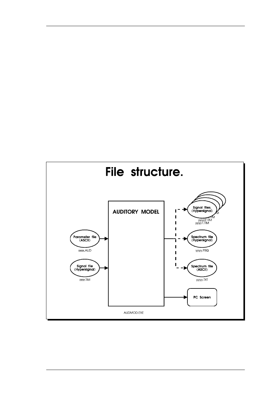
8.1
User manual.
The auditory model has been written in the C language and compiled and debugged
using the Borland Turbo C++ 1.0 compiler. It runs on any IBM PC-AT compatible
computer with a mathematical co-processor. For processing of long signals, at least a
386DX - 25 MHz is recommended due to the heavy computation load in the model. The
entire model is contained in a single executable, AUDMOD.EXE, which is provided on a
disk along with a few sample input parameter files. The flow of the program is
illustrated in figure 26.
26.
Block-diagram indicating the file structures and data flow in the auditory model. Two input files
are required: .AUD parameter file and .TIM signal file. The model output is sent to the screen
(can be redirected to a file) and to an output file in either Hypersignal binary format (.FRQ) or in
an ASCII text file (.TXT).
8
Appendices.
An auditory model with hearing loss.
Page 81
8. Appendices

8.1.1 Input parameter file format.
The .AUD input parameter file specifies all the free parameters in the model. These
parameters must be in a particular order, as shown below. A line that begins with a
non-white character (i.e. not a tab, space or new line character) is considered an input
line, whereas a line beginning with a white character is ignore. All indented lines can
thus be used for comments. A valid input line requires the accurate spelling of the
parameter, followed by one or more tabs and/or spaces, and the value of the parameter.
A sample parameter file is shown in figure 27.
Page 82
An auditory model with hearing loss.
8. Appendices

AUDITORY MODEL PARAMETERS
Filename:
test41.aud
Date:
28.12.92
Time:
15:00
Notes:
30 channel FFT-based model, using roex filters.
Excitation patterns, white noise, 10 db steps
All indented lines are ignored.
Model parameters follow in order:
No. channels:
30
Lower E limit:
3
Upper E limit:
32
Output channel:
0
0 for all channels.
Output level:
0
0 for end of model.
Input sample rate (Hz):
20000
dB SPL of cal. sinus:
60
Peak value of cal. sin:
16358
sqr(2)*noise signal rms value
Recording coupler:
1
1: Free field, 2: IEC711/KEMAR, 3: IEC303
Transmission factor:
1
1: Zwicker's A0, 2: ELC 100, 3: ELC100 flat bl. 1 kHz
Binaural:
0
0: Monaural, else binaural loudness
Output sample rate(Hz):
0
If 0, based on input sample rate, frame size and
overlap
Input frame size:
256
Must be power of two and no more than 8192
Overlap:
0
No overlap
Process:
8
0 = all frames, 1 = single frame, n = #frames to
average
Output frame size:
100
No. frames to process:
0
0 for all frames.
No. zero frames to add:
0
The input signal can be padded with zeros
if model has post-masking.
Output format:
11
Can be 1 time series per file:
or output as vectors:
Hypersignal FRQ (10), int (11) or float (12)
Audiogram (Hz):
125
250
500
750
1000
1500
2000
3000
4000
6000
8000
Audiogram (dB HL):0
0
0
0
0
0
0
0
0
0
0
UCL (dB HL):
120
120
120
120
120
120
120
120
120
120
120
27.
Sample parameter file for auditory model. All indented lines are ignored by the model, serving as
comments.
Since all indented lines are ignored by AUDMOD.EXE, the first few lines in figure 27
are comments to aid the user. The input parameters then follow:
1.
No. channels: Number of output channels in the auditory model. The
spacing between the channels in E-units is determined by the upper and
lower limits on the E-scale as defined in the following two parameters.
An auditory model with hearing loss.
Page 83
8. Appendices

The number of channels has been 30 in the current report corresponding to
roughly 7 kHz bandwidth in the model. In the case of an .FRQ output file,
the number of channels is rounded up to nearest power of two plus one
(i.e. 33 channels), and the E-spacing is consequently reduced.
2.
Lower E limit: The center E-value for the lowest band in the model. E =
3 corresponds to 87 Hz.
3.
Upper E limit: The center E-value for the highest band in the model. E
= 32 corresponds to 6.97 kHz.
4.
Output channel: Only relevant in the case of the output being specified
as one waveform file per channel (Output format: 0). One particular
channel can be selected here, if the other waveform files are irrelevant.
Usually set to 0, meaning that all channels are output.
5.
Output level: This specifies at which point in the model, the output
frames are written to the output file as follows (see figure 1):
5: ERB-power
6: Excitation from roex filterbank (E).
7: Specific loudness = end of model.
0: End of model. (could change in the future).
6.
Input sample rate: Sample rate for input file. Normally overridden by
the sample rate specified in the input waveform (.TIM) file header. Can be
checked on the output screen from the model.
7.
dB SPL of cal. sinus: For absolute sound pressure level calibration of the
model. Assume, for example, that we have recorded a calibration sine
wave to a waveform file using the same electrical gain from the
microphone to the A/D-converter as used for recording of the signals for
analysis. The actual dB SPL value of the calibration signal (typically 94
dB SPL, for a B&K 4230 calibrator) read from the measurement amplifier
should then be written down and entered here. The dB SPL parameter can
also be used for 'artificial' signals or to scale signals up or down to force a
given dB SPL-calibration.
8.
Peak value of cal. sinus: From the above example, the peak value of the
sine wave in the signal file must then be determined. This can be done in a
signal-editor (such as HyperSignal Workstation) or by means of a
peak-detecting program. If the signal is noisy, or not a sine wave, this
peak value cannot be estimated easily. In this case, it is better to
determine the long-term RMS-value and multiply it by
. The small
2
utility RMS.EXE (Nielsen, 1992) can be used to calculate RMS- and peak
values for Hypersignal .TIM waveform files.
Page 84
An auditory model with hearing loss.
8. Appendices

By means of parameters 7. and 8. a signal can be set to the desired
SPL-value by determining the long-term RMS-value of the signal file,
multiply by
to get parameter 8, and setting the dB SPL (parameter 7)
2
to the desired value.
9.
Recording coupler: If a signal was recorded by means of a microphone,
the auditory model must know at which point the signal was recorded.
There are three options available, which are set by numerical value:
1: Recorded in free field (or reverberant), i.e. a microphone in a room.
2: Recorded at the eardrum, in KEMAR, or in an IEC 711 ear simulator.
3: Recorded in an IEC 303 (6 cm
3
) coupler.
Most real-world or synthetic signals should be referred to free-field (1), as
they were recorded in a room, or assumed to be reproduced by a
loudspeaker with a flat frequency response. If the signal is referred to the
eardrum (e.g. the tympanic membrane, parameter value 2), the auditory
model must divide the input spectrum by the open-ear response. Similarly,
a coupler frequency response correction is applied in the case of an IEC
303 coupler (value 3). See section 3.3 for further discussion on coupler
corrections.
10. Transmission factor: Specifies the fixed frequency response equalization
applied to the input spectrum (after correcting for coupler response)
before passing it through the auditory filterbank. The parameter choices
are:
1: Zwicker a
0
transmission factor.
2: 100-phone equal-loudness contours.
3: 100-phone equal-loudness contours, flat below 1 kHz.
See section 3.3 for details.
11. Binaural: For selection of monaural or binaural listening. Monaural (0)
is obviously used for eardrum recordings or with hearing aid. The binaural
(1) condition applies to a symmetric binaural situation, ie. symmetric
hearing loss listening in the vertical plane only (azimuth = 0).
12. Output sample rate (Hz): Specifies the sample rate, i.e. the time
intervals between successive output frames. This is accomplished by
forcing the overlap between input frames to the right value. By setting the
output sample rate to 0, it will instead be calculated based on sample rate,
input framesize and overlap and forced to this value.
13. Input frame size: The width, in samples, of successive input frame. Due
to the FFT used for calculation of the spectrum, the frame size must be a
power of two from the following set of values: 128, 256, 512, 1024,
An auditory model with hearing loss.
Page 85
8. Appendices

2048, 4096, 8192. For the simulations in this model, 256 point frames
were used, corresponding to 12.8 ms frame width at 20 kHz sample rate.
14. Overlap: The overlap, in samples, between successive input frames. 0
means no overlap, i.e. the input frames are side-by-side. The highest value
is input frame size - 1, corresponding to a 1 sample increment in the input
signal after reading a new frame. For 75% overlap, which was used for
the speech signals in section 5.1., the overlap value must be set to 192.
15. Process: Used to specify an optional spectral averaging. 0 means that all
frames average into one long-term power spectrum. Useful for stationary
noise signals. 1 means single frame, i.e. no averaging. Any other positive
integer specifies the number of successive input frames to be averaged into
1 output frame. For instance, 8 means that 8 input frames at a time are
averaged to form one output frame.
16. Output frame size: For time-domain output files, (Output format 0), this
is the frame size of each output file. In the case of frequency-domain files
(Output format 10 or 11), this specifies how many frames are stored
internally, before being written to file. In the latter case, this number is not
critical, and a typical value of 100 can easily be used without any memory
problems.
17. No. frames to process: Number of input frames to process, before
terminating program. 0 means the entire input file, any other number is
used to specify a smaller number of frames, ie. not the entire file.
18. No. zero frames to add: Optional number of frames containing zeros,
that are padded to the input signal file. Useful for a future version of the
model that contains post-masking, so that the model is allowed to settle
after the input signal has been turned off.
19. Output format: Three choices are available for output file formats:
0: .TIM time-domain waveform files, with one channel per file. For N
channels, N output files are created, using the first six letters of the output
file name plus two digits to form the file name XXXXXXNN.TIM, where
NN is the channel number of the output file. These files are in
HyperSignal Workstation format, where they can be viewed and
manipulated.
10: .FRQ frequency domain files with consecutive frames stored in one
file. Each output 'spectrum' is stored as a 16-bit integer value in a frame.
The file can be viewed and manipulated further in HyperSignal
Workstation. The speech processing examples in figures 23, 24 and 25
have been made from Hypersignal screen outputs.
Page 86
An auditory model with hearing loss.
8. Appendices

11: .TXT text output files: This file contains header information,
followed by channel information (E-value, center frequency), followed by
the actual data, frame-by-frame. For each frame, separate lines are printed
for the ERB-power, the filterbank output (excitation), and specific
loudness. The output file can be imported into a spreadsheet, such as
Microsoft Excel, with each line forming one row. The data values in the
.TXT file are delimited by tab characters, which is converted into separate
columns in Excel.
20. Audiogram (Hz): The audiogram frequencies, listed in order. In the
current implementation, these are not optional, but must be (in order):
125, 250, 500, 750, 1000, 1500, 2000, 3000, 4000, 6000, 8000. In the
case of missing intermediate frequencies, these can be interpolated on an
audiogram form.
21. Audiogram (dB HL): The hearing loss at each of the audiogram
frequencies listed above. Normal hearing corresponds to 0 dB HL for all
frequencies.
22. UCL (dB HL): The uncomfortable levels at each of the audiogram
frequencies, expressed in dB HL. This line must be included, but the
proposed UCL encoding scheme (Appendix 8.2) has not been evaluated.
The UCL effect can effectively be disabled by specifying large values, e.g.
120 dB HL across all frequencies.
8.1.2 Command-line usage.
Many of the input file parameters can be overridden on the DOS command-line. The
command-line format is the following:
AUDMOD parmfile infile outfile [switches]
where
parmfile
is the auditory model parameter file base name (see above for format).
The file extension .AUD should not be included, since it is added by the program
automatically.
infile
is the input waveform file (.TIM - Hypersignal format). The file extension
.TIM should not be included, since it is added by the program automatically.
An auditory model with hearing loss.
Page 87
8. Appendices

outfile
is the output file base name. In the case of time waveform output files
(Output format 0), the base name is truncated to 6 letters, and the remaining two
characters are used for channel numbering. The file extension .TIM is appended
automatically. In the case of spectrum output files (.FRQ - format 10 or .TXT -
format 11), there is only one output file, and the appropriate file extension is
appended automatically.
The optional command-line switches are listed in Figure 28. In the cases where they
duplicate parameter file values, the command-line values are used.
AUDMOD : Auditory model signal processing.
Copr.(C) Lars Bramsløw Nielsen
Revision: 1.3 Date: Jan 15 1993
Usage : AUDMOD parmfile infile outfile [switches]
parmfile: ASCII file with model setup parameters (.AUD)
infile: HS time series file containing input signal (.TIM)
outfile: HS time series file name for output (max. 6 char)
2 digits appended for channel number
Optional processing switches override parmfile setttings:
/c#: Channel signal to be output, default all channels.
/l#: Output level in model, 1 = first stage etc.. , 0 = all.
/o#: Output format, 0 = .TIM, 10 = .FRQ.
/f#: Number of frames to process, default all.
/s#: Framesize, 128 - 8192 (power of two).
/t#: Number of milliseconds to process, default all.
/p#: Spectrum processing: 0 = single frame,
1 = power spectrum averaging.
/b#: Binaural/Monaural loudness: 0 = Mon., 1 = Bin.
/d : Debug mode - print more info.
28.
AUDMOD help screen specifying the required file names and the optional command-line
parameters.
Assuming that all values in the parameter file are specified correctly, the model can be
run on a given input signal. There are self-explanatory error-messages in the case of
illegal input file format or incorrect or conflicting input parameter values. A typical
session then produces the screen output shown in Figure 29:
Page 88
An auditory model with hearing loss.
8. Appendices

C:\DSP\AUDMOD\EVAL>audmod test41 uen_2db jtest > audmod.out
AUDMOD : Auditory model signal processing.
Copr.(C) Lars Bramsløw Nielsen.
Revision: 1.3 Date: Dec 28 1992
------------------------- Processing Parameters -------------------------
Parameter file: test41.AUD Recording coupler: Free field
Signal file: uen_2db.TIM Transmission factor: a0 (Zwicker)
Output file(s): test Monaural loudness.
Input sample rate: 20000.0 Hz Input frame size: 256
Overlap: 0 Number of input frames: 208
Spectrum averaging: 8 frames.
Number of channels: 30 Output channel: All
E-start, E-end: 3.0, 32.0 E-step: 1.000
Output sample rate: 78.1 Hz
Output level: End of model. Output format: 11
Hit 'Esc' to terminate processing.
Frame #
8.
Power:
1.58
dB SPL
Loudness:
0.000
son
Frame #
16.
Power:
3.50
dB SPL
Loudness:
0.000
son
Frame #
24.
Power:
1.58
dB SPL
Loudness:
0.000
son
Frame #
32.
Power:
3.50
dB SPL
Loudness:
0.000
son
Frame #
40.
Power:
5.67
dB SPL
Loudness:
0.000
son
Frame #
48.
Power:
7.20
dB SPL
Loudness:
0.000
son
Frame #
56.
Power:
9.40
dB SPL
Loudness:
0.000
son
Frame #
64.
Power:
11.33
dB SPL
Loudness:
0.000
son
Frame #
72.
Power:
13.01
dB SPL
Loudness:
0.000
son
Frame #
80.
Power:
15.43
dB SPL
Loudness:
0.000
son
Frame #
88.
Power:
17.34
dB SPL
Loudness:
0.000
son
Frame #
96.
Power:
18.98
dB SPL
Loudness:
0.000
son
Frame #
104.
Power:
21.30
dB SPL
Loudness:
0.003
son
Frame #
112.
Power:
23.63
dB SPL
Loudness:
0.041
son
Frame #
120.
Power:
25.85
dB SPL
Loudness:
0.112
son
Frame #
128.
Power:
27.66
dB SPL
Loudness:
0.175
son
Frame #
136.
Power:
29.95
dB SPL
Loudness:
0.312
son
Frame #
144.
Power:
31.36
dB SPL
Loudness:
0.418
son
Frame #
152.
Power:
34.00
dB SPL
Loudness:
0.641
son
Frame #
160.
Power:
35.39
dB SPL
Loudness:
0.819
son
Frame #
168.
Power:
36.79
dB SPL
Loudness:
0.998
son
Frame #
176.
Power:
39.36
dB SPL
Loudness:
1.363
son
Frame #
184.
Power:
41.59
dB SPL
Loudness:
1.715
son
Frame #
192.
Power:
43.33
dB SPL
Loudness:
2.055
son
Frame #
200.
Power:
45.22
dB SPL
Loudness:
2.498
son
Frame #
208.
Power:
47.10
dB SPL
Loudness:
2.942
son
Frame #
216
Power:
50.16
dB SPL
Loudness:
3.782
son
Frame #
224
Power:
51.22
dB SPL
Loudness:
4.153
son
Processing completed.
29.
Typical screen output from the auditory model. The output can be directed to a file, and columns
are separated by Tab's to facilitate import into a spreadsheet.
The screen output can be redirected to a file in the usual DOS manner:
AUDMOD parmfile infile outfile [switches] > scrnfile
An auditory model with hearing loss.
Page 89
8. Appendices

In this file, the columns are separated by tab characters, for easy import into a
spreadsheet. The redirection does not apply to error messages, thus these are always
forced to the screen (stderr, in UNIX and C terms).
8.2
Proposed UCL-encoding.
This encoding has been implemented in the model but has not been evaluated. The data
from Allen et al (1990) show a steeper section on the average loudness growth curve for
normal hearing subjects above the LOUD rating (= 6, equivalent to app. 50 sones). A
similar pattern appears for individual hearing-impaired listeners. The standard loudness
curve is thus modified by adding a steep, almost vertical, section to the specific loudness
curve near UCL:
N
UCL
Â
=
N
Â
1
−
E
EUCL
1
0.23
(23)
The modification, implemented in the denominator approaches zero rapidly when E
approaches E
UCL
. The exponent 1/0.23 has been chosen somewhat arbitrarily to obtain a
sharp transition close to UCL.
The values of E
UCL
are found in the same fashion as for E
TQ
, by presenting a shaped
spectrum equivalent to the pure-tone UCLs. As for threshold values, discrepancies
between the simultaneously presented UCL-shaped spectrum and the UCL measurement
procedure with one tone presented at a time may be of importance here. The UCL
feature has been implemented, but not tested against experimental data.
Page 90
An auditory model with hearing loss.
8. Appendices
Wyszukiwarka
Podobne podstrony:
NASA 98 acc eam GLOBAL NONLINEAR PARAMETR MODEL WITH APP TO F 16 AERODYNAMICS
Modeling computer virus prevalence with a susceptible infected susceptible model with reintroduction
Coping with Vision Loss Understanding the Psychological, Social, and Spiritual Effects by Cheri Colb
Dornbusch Fischer Samuelson Comparative Advantage, Trade, and Payments in a Ricardian Model with a
multiplex PCR and minisequencing of SNPs a model with 35 Y chromosome SNPs(1)
Farina Reproduction of auditorium spatial impression with binaural and stereophonic sound systems
0502 Refrigerant circuit Model 126 with air conditioning system
Farina Reproduction of auditorium spatial impression with binaural and stereophonic sound systems
General Training Reading Chinese Stretch to Catch up with Teenage Model
Ebsco Nolen Hoeksema Ruminative Coping With Depressed Mood Following Loss
Greater weight loss and hormonal changes after 6 months diet with carbohydrates eaten mostly at dinn
Model for energy conversion in renewable energy system with hydrogen storage
Parameters od model luminaire with high power LED diodes
Fast food diet model of NASH with ballooning, progressive fibrosis, and high physiological fidelity
Kim Control of auditory distance perception based on the auditory parallax model
Distributed Worm Simulation with a Realistic Internet Model
więcej podobnych podstron