18

P. HAZDRA, M. MAZÁNEK, L-SYSTEM TOOL FOR GENERATING FRACTAL ANTENNAS STRUCTURES WITH ABILITY …

L-System Tool for Generating Fractal Antenna

Structures with Ability to Export into EM Simulators

Pavel HAZDRA, Miloš MAZÁNEK

Department of Electromagnetic Field, Czech Technical University, Technická 2, 166 27 Praha, Czech Republic

[e-mail], [e-mail]

Abstract. An L-System (Lindenmayer system) is a scheme
primarily developed in the area of the computer science for
simulating the development of biological structures. It has
also been found very useful for generating the geometry of
various fractal antennas. A Matlab environment has been
used for both implementing an in-plane L-systems algo-
rithm and for creating appropriate files for widely used
EM simulators like the IE3D and the CST Microwave
Studio. Finally, the performance of the developed script is
demonstrated on two fractal microstrip patch antennas.

Keywords

Fractal antennas, fractals, L-Systems, EM simulation,
microstrip patch antennas.

1. Introduction

In computer science terms, an L-System [1] is a con-

text-free, recursive, text substitution scheme, followed by
a geometric interpretation. A simple L-System starts with
a seed S, say the letter F, and has one or more rules R1 to
Rn to replace the initiatory seed. A simple replacement rule
might be, for example R: F→F−F−FF+F−F−F (meaning of
used characters is described later in detail).

The rule is then recursively applied many times (de-

pending on the desired iteration level) to produce a series
of strings of the increasing complexity. In order to produce
fractals, the strings generated by L-Systems have to contain
the necessary information about the figure geometry.
A graphic interpretation of strings is based on assigning the
language to the motion of an imaginary turtle. This inter-
pretation is used to produce fractal images [2] and has been
implemented in our Matlab script. Examples are given be-
low together with an explanation of the L-System language
alphabet.

2. L-System Language

Let us describe the specific language (alphabet) used

in the presented simple L-System Matlab script.

F move forward a step of the length d;
+ turn to the left by a specified angle θ;
− turn to the right by a specified angle θ.

Moreover, advanced letters are also defined with the fol-
lowing meanings:

G move forward a step of length e;
> turn to the left by a specified angle φ;

< turn to the right by a specified angle φ;

[ push the current state of the turtle onto a stack;

] pop a state from the stack and make it the current sta-

te of the turtle.

The last two letters allow us to make a so-called bracketing
string [2] resulting in branched structures (tree like).

In order to make the usage of the script more conve-

nient, and in accordance with a common notation [2], some
advanced letters are implemented:

L =

+F−F−F+

R =

−F+F+F−

D =

−−F++F

E =

F−−F++

X, Y = do nothing

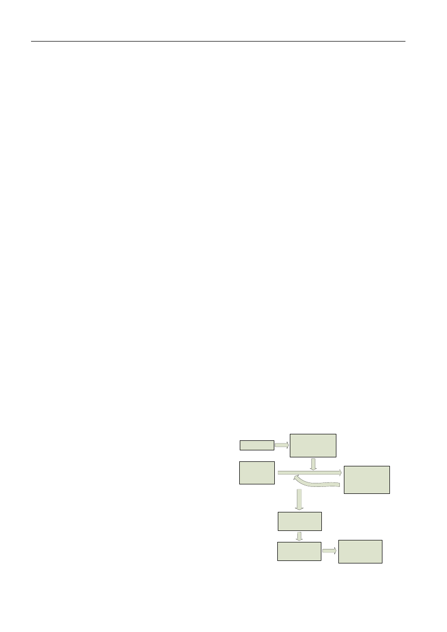
Start with

axiom

F

Apply the rule (replace

the F letter by the

following)

F - - > F-F++F-F

Get new string, after 1

st

iteration it would be:
F+F--F+F+F+F--F+F--
F+F--F+F+F+F--F+F

Repeat the rule until

desired iteration level

Given iteration

level reached

theta = 60

°

Convert the

generated string into
vector of (x,y) points

Convert the

generated string into

vector of (x,y) points

Add a z coordinate,

create matrix of (x,y,z)

points and export it as

a .3dt file for IE3D

Fig. 1. A flowchart showing the script generating the Koch curve.

RADIOENGINEERING, VOL. 15, NO. 2, JUNE 2006

19

Fig. 1 shows a flowchart demonstrating how the

script generates the Koch curve as one of the simplest
examples.

Although the above described alphabet is very simple,

it allows us to create quantities of various fractals which
are discussed in the following section.

3. Examples

Fractals can be generally divided into 3 different

groups according to their geometrical properties. Our
L-System generator is able to create all kinds of fractals in
the XY plane. Let us imagine a fractal set R with Hausdorff
[2] interior dimension D. Dimension of the boundary ∂R
will be denoted d. Then:

a) D is an integer and d is a non-integer, respectively.

A planar object with a fractal boundary like the Koch
snowflake, where D = 2 and d ~ 1.26, is an example.

b) d is an integer and D < 2 is a non-integer, resp. Frac-

tal curves like the Minkowski (D = 1.5) and the Koch
(D = 1.26) belong to this group. Also fractal trees
satisfy these conditions.

c) Both d and D are non-integers. A porous material or

a natural snowflake are examples.

In the following section, some examples of the script capa-
bility are shown.

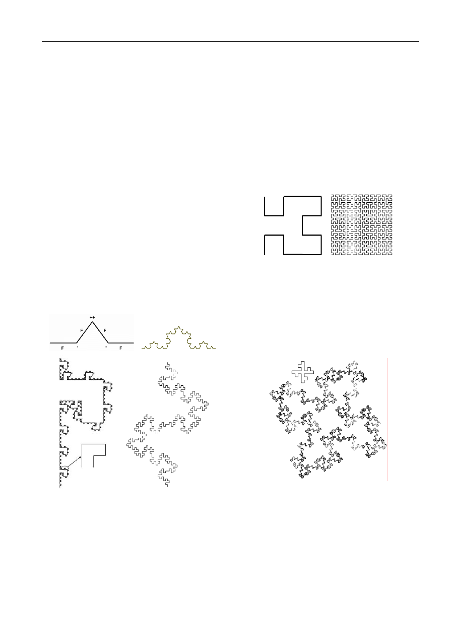
Fig. 2. Generation of Koch Curve (top), Coastline (bottom left)

and Minkowski Curve (bottom right), both iteration 3.

3.1 Fractal Curves

• Koch Curve

S: F
R: F→F−F++F−F, θ=60

°

see Fig. 2 (at the top) for generating process details.

• Coastline

S: F
R: F→FFFF+F+F−F−FF−FF+F, θ=90

°

see Fig. 2 (three iterations performed).

• Minkowski Curve

S: F
R: F→F−F+F+FF−F−F+F, θ=90

°

see Fig. 2 (three iterations performed).

• Hilbert Curve

S : L
R1: L→+RF−LFL−FR+, θ=90

°

R2: R→−LF+RFR+FL, θ=90

°

see Fig. 3 for Hilbert Curve, 1 and 4 iterations shown.

Fig. 3. Hilbert Curve, iteration 1 and 4.

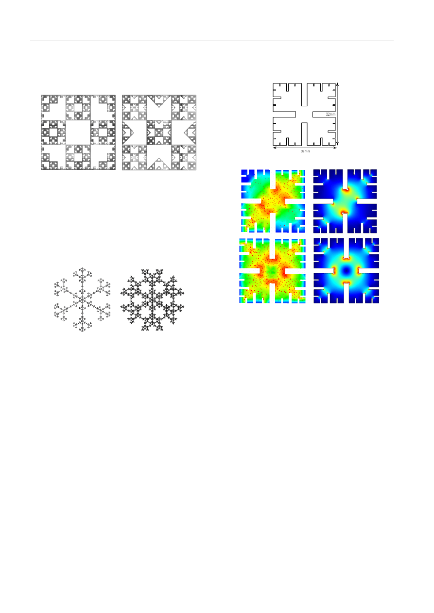
3.2 Planar Closed Sets with a Fractal

Boundary

• Quadratic Koch Island

S: F+F+F+F
R: F→F−F+F+FFF−F−F+F,
θ=90

°

, see Fig. 4 (three iterations performed).

Fig. 4. Quadratic Koch Island, iteration 3. Iteration 1 shown also

for the comparison.

3.3 Other Planar Fractals

• Tegel I

S: F−F−F−F
R: F→FF[−F−F−F]F, θ=90

°

see Fig. 5 (left).

20

P. HAZDRA, M. MAZÁNEK, L-SYSTEM TOOL FOR GENERATING FRACTAL ANTENNAS STRUCTURES WITH ABILITY …

• Tegel II

S: F−F−F−F
R: F→F[−F+F+F]FF, θ=90

°

see Fig. 5 (right).

Fig. 5. Tegel I and Tegel II, iteration 4.

• Snowflake I

S: [F]+[F]+[F]+[F]+[F]+[F]
R: F→FF[+F][ −F]F, θ=60

°

see Fig. 6 (left).

• Snowflake II,

S: [F]+[F]+[F]+[F]+[F]+[F]
R: F→FF[+F−F][ −F+F]F, θ=60

°

see Fig. 6 (right).

Fig. 6. Snowflake I and Snowflake II, iteration 4.

4. Applications

The main purpose of the presented generator is to stu-

dy various fractal antennas using numerical EM simulation.
Let us consider a fractal patch of the iteration 3 (Fig. 7) de-
fined as follows:

• S : F+F+F+F

R1: F→FF+GGGG−G−GGGG+F
R2: G→GGG
d = 1, e = 0.1, θ = φ = 90

°

The Matlab script produces the antenna geometry in a .3dt
format which can be directly imported to the full wave
simulator IE3D. The simulation was carried out with the
infinite ground-plane, the air substrate h = 1 mm and was
fed by a coaxial probe. The antenna’s first resonance ap-
peared at 3 GHz, which is approximately 65 % reduction in
frequency compared to a square patch of the same outer
dimensions. This is addressed by the fact that the fractal
geometry forces currents to flow along the patch’s diagonal
(see Fig. 8a). For verification purposes, modal currents
have been calculated by using the cavity model theory [3],

[4] implemented in the Femlab software. Except for the
fundamental mode #1, the mode #4 is also shown to check
the agreement between 2 different simulation approaches.

Fig. 7. Fractal patch antenna created by our L-system script.

a)

b)

Fig. 8. Mode #1 and #4 current densities calculated by the full-

wave model and the cavity one: a) mode #1, full-wave IE3D
(left), cavity FEMLAB (right), b) mode #4, full-wave IE3D
(left), cavity FEMLAB (right).

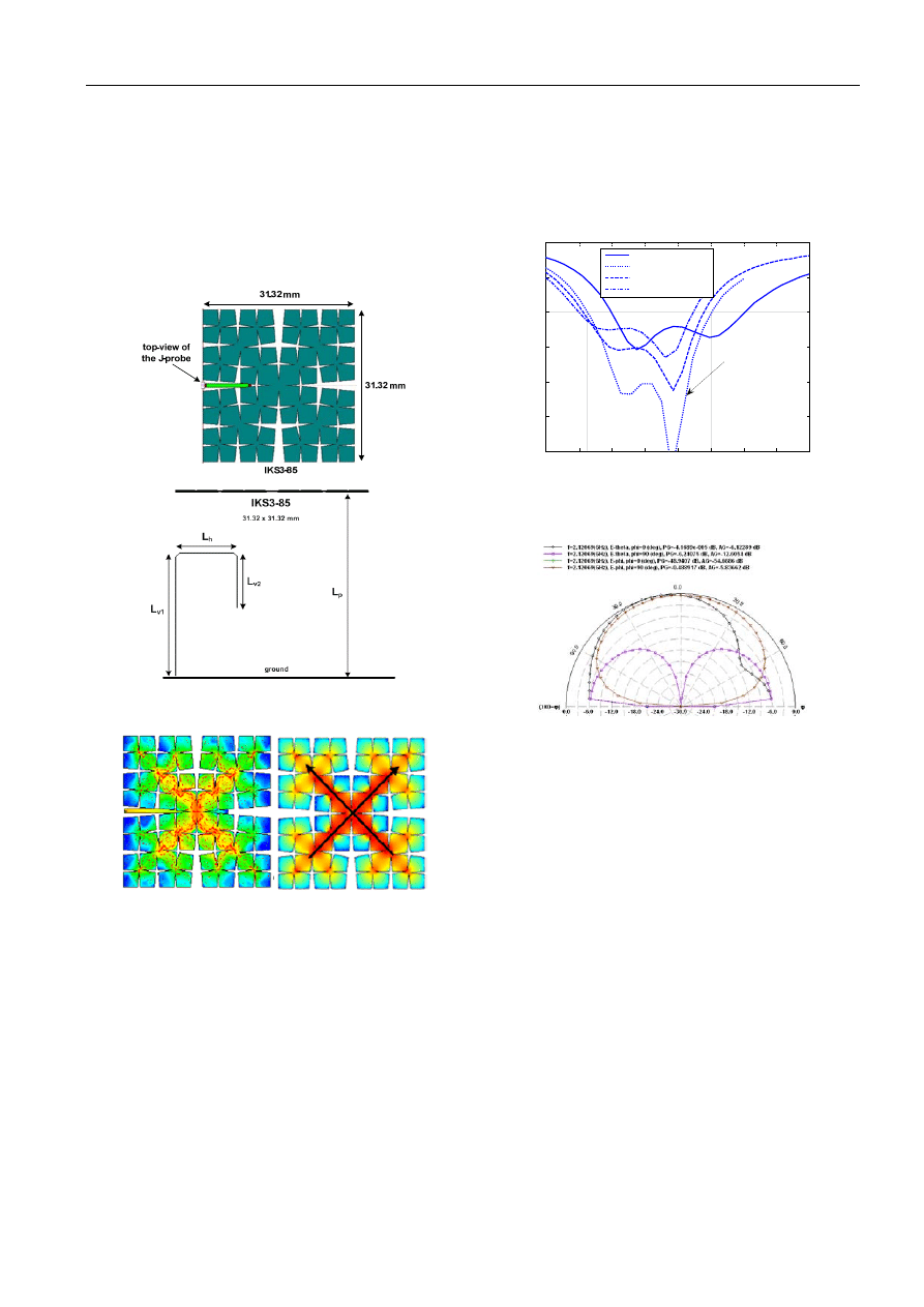
Another interesting antenna structure created with the
L-System described is a so-called Inverted Koch Square
patch [5]. The structure is obtained by the following ruling:

• S: F<F<F<F

R: F→F−F++F−F.

We use the notation IKSn-α-J (n stands for the number of
performed iterations, α is so-called indentation angle [5], J
denotes that the J-probe is used as the feeding system). The
indentation angle α is defined within the operators + and –.
The seed is a rectangle, the angle for the operator < is thus
β = 90°. For the analysis, IKS3-85-J is selected (Fig. 8).

First, the modal analysis is employed to predict reso-

nances and surface currents, and the fundamental mode
with the lowest resonant frequency is chosen. The modal
estimation predicts the resonant frequency to be lower,
~ 30 % of the rectangular patch antenna with the same
edge dimensions (31.32mm

× 31.32mm). The comparison

of surface currents obtained from full-wave analysis and
the modal one is shown in Fig. 9. Arrows clearly show two
main current paths, both being in-phase. Thus, the expected
radiation pattern should be broadside.

Second, the suitable feeding technique is employed to

provide the appropriate matching. We use the so-called J-

RADIOENGINEERING, VOL. 15, NO. 2, JUNE 2006

21

probe (see Fig. 8) and adjust the main parts of the probe
using the parametric IE3D full-wave simulation. A partial
result of the parametric study performed is shown in Fig.
10, the final dimensions of the J-probe are L

v1

= 20 mm,

L

h

= 10 mm, L

v2

= 8 mm, L

p

= 30 mm resulting in a relative

frequency bandwidth of 18 %. Let us note that dimensions
of the edges are 0.22 λ

× 0.22 λ, thus the antenna is notably

smaller than the conventional rectangular patch antenna
operating at fundamental “0.5 λ“ mode.

Fig. 8. Layout of the IKS3-85-J antenna, top and side view.

Fig. 9. IKS3-85-J. Surface currents at the fundamental mode –

full wave results (left), modal analysis (right).

The antenna exhibits directivity of 4.5 to 6.6 dBi across the
working band, the radiation pattern at the central frequency
is shown in Fig. 11. A more detailed discussion on radia-
tion properties could be found in [5].

5. Conclusion

This paper presents a widely configurable fractal

geometry generator based on an L-System algorithm im-
plemented in a Matlab environment. Various outputs from
the generator are shown together with the simplicity of
entering the input data. The script is ready to be used with-

in the optimization loop as all the parameters are simple to
access and with clear impact on the generated geometry.
Future plans are to use the modal analysis together with the
described generator to optimize the frequency response of
planar fractal antennas. Finally, two examples of microstrip
fractal patch antennas created with the script are given.

1.8

1.9

2

2.1

2.2

2.3

2.4

2.5

2.6

-30

-25

-20

-15

-10

-5

0

f [GHz]

RL [

d

B

]

Lv1=20,Lh=10,Lv2=5

Lv1=20,Lh=10,Lv2=8
Lv1=20,Lh=10,Lv2=9

Lv1=20,Lh=10,Lv2=10

Lv1=20, Lh=10, Lv2=8

Fig. 10. Return loss of IKS3-85-J antenna with L

v1

= 20 mm,

L

h

= 10 mm, L

p

= 30 mm, L

v2

being variable.

Fig. 11.

Two principal far-field cuts @ 2.12GHz for IKS3-85-J,

L

v1

= 20 mm, L

h

= 10 mm, L

v2

= 8 mm, L

p

= 30 mm.

Acknowledgements

Research described in the paper was supported by the

grant 102/03/H086 Novel Approach and Coordination of
Doctoral Education in Radioelectronics and Related Disci-
plines and by the Research program MSM 202300014.

References

[1] http://en.wikipedia.org/wiki/L-system

[2] PEITGEN, O., JURGENS, H., SAUPE, D. Chaos and Fractals, 2

nd

ed. Springer-Verlag. 2004.

[3] BAHL, I., GBARTIA, P., GARG, R., ITTIPIBOON, A. Microstrip

Antenna Design Handbook. Artech House, 2001

[4] HAZDRA, P., MAZÁNEK, M. On the modal analysis of fractal

microstrip patch antennas. In Radioelektronika 2004 Conference
Proceedings. Bratislava: STU Bratislava, 2004.

[5] HAZDRA, P., MAZÁNEK, M. The miniature fractal patch antenna.

In Radioelektronika 2005 Conference Proceedings. Brno: Brno Uni-
versity of Technology, 2005, p. 207–210. ISBN 80-214-2904-6.