Two Dimensional Truss
Introduction
This tutorial was created using ANSYS 7.0 to solve a simple 2D Truss problem. This is the first of four
introductory ANSYS tutorials.
Problem Description
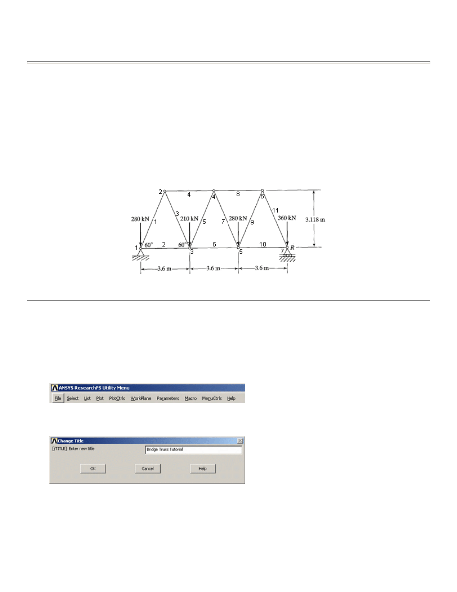
Determine the nodal deflections, reaction forces, and stress for the truss system shown below (E = 200GPa, A =
3250mm
2
).
(Modified from Chandrupatla & Belegunda, Introduction to Finite Elements in Engineering, p.123)
Preprocessing: Defining the Problem
1. Give the Simplified Version a Title (such as 'Bridge Truss Tutorial').
In the Utility menu bar select File > Change Title:
The following window will appear:
Enter the title and click 'OK'. This title will appear in the bottom left corner of the 'Graphics' Window
once you begin. Note: to get the title to appear immediately, select Utility Menu > Plot > Replot
2. Enter Keypoints
The overall geometry is defined in ANSYS using keypoints which specify various principal coordinates
University of Alberta ANSYS Tutorials - www.mece.ualberta.ca/tutorials/ansys/BT/Truss/Truss.html
Copyright © 2002 University of Alberta
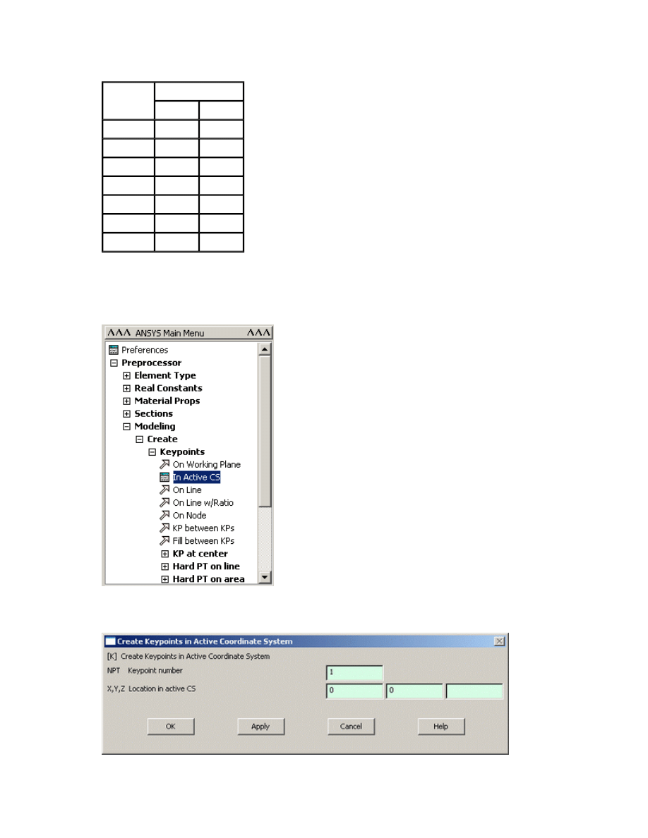
to define the body. For this example, these keypoints are the ends of each truss.
{
We are going to define 7 keypoints for the simplified structure as given in the following table
(these keypoints are depicted by numbers in the above figure)
{
From the 'ANSYS Main Menu' select:
Preprocessor > Modeling > Create > Keypoints > In Active CS
The following window will then appear:
{
To define the first keypoint which has the coordinates x = 0 and y = 0:
keypoint
coordinate
x
y
1
0
0
2
1800
3118
3
3600
0
4
5400
3118
5
7200
0
6
9000
3118
7
10800
0
University of Alberta ANSYS Tutorials - www.mece.ualberta.ca/tutorials/ansys/BT/Truss/Truss.html
Copyright © 2002 University of Alberta
Enter keypoint number
1
in the appropriate box, and enter the x,y coordinates:
0, 0
in their
appropriate boxes (as shown above).
Click 'Apply' to accept what you have typed.
{
Enter the remaining keypoints using the same method.
Note: When entering the final data point, click on 'OK' to indicate that you are finished entering
keypoints. If you first press 'Apply' and then 'OK' for the final keypoint, you will have defined it
twice!
If you did press 'Apply' for the final point, simply press 'Cancel' to close this dialog box.
Units
Note the units of measure (ie mm) were not specified. It is the responsibility of the user to ensure that a
consistent set of units are used for the problem; thus making any conversions where necessary.
Correcting Mistakes
When defining keypoints, lines, areas, volumes, elements, constraints and loads you are bound to make
mistakes. Fortunately these are easily corrected so that you don't need to begin from scratch every time an
error is made! Every 'Create' menu for generating these various entities also has a corresponding 'Delete'
menu for fixing things up.
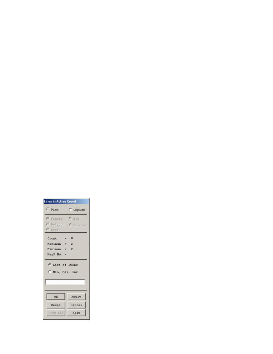
3. Form Lines
The keypoints must now be connected
We will use the mouse to select the keypoints to form the lines.
{
In the main menu select: Preprocessor > Modeling > Create > Lines > Lines > In Active Coord.
The following window will then appear:
{
Use the mouse to pick keypoint #1 (i.e. click on it). It will now be marked by a small yellow box.
University of Alberta ANSYS Tutorials - www.mece.ualberta.ca/tutorials/ansys/BT/Truss/Truss.html
Copyright © 2002 University of Alberta
{
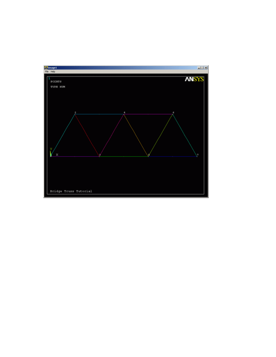
Now move the mouse toward keypoint #2. A line will now show on the screen joining these two
points. Left click and a permanent line will appear.
{
Connect the remaining keypoints using the same method.
{
When you're done, click on 'OK' in the 'Lines in Active Coord' window, minimize the 'Lines' menu
and the 'Create' menu. Your ANSYS Graphics window should look similar to the following figure.
Disappearing Lines
Please note that any lines you have created may 'disappear' throughout your analysis. However, they have
most likely NOT been deleted. If this occurs at any time from the Utility Menu select:
Plot > Lines
4. Define the Type of Element
It is now necessary to create elements. This is called 'meshing'. ANSYS first needs to know what kind of
elements to use for our problem:
{
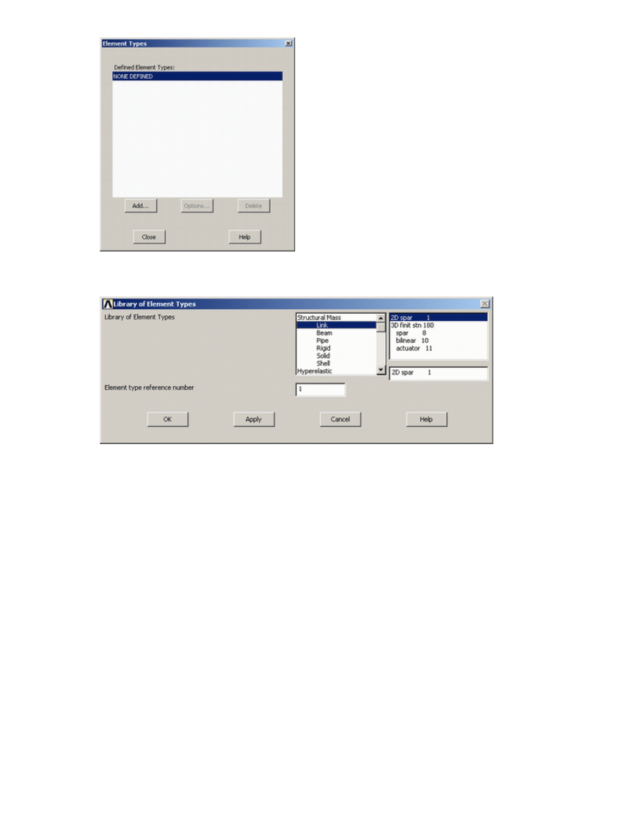
From the Preprocessor Menu, select: Element Type > Add/Edit/Delete. The following window
will then appear:
University of Alberta ANSYS Tutorials - www.mece.ualberta.ca/tutorials/ansys/BT/Truss/Truss.html
Copyright © 2002 University of Alberta
{
Click on the 'Add...' button. The following window will appear:
{
For this example, we will use the 2D spar element as selected in the above figure. Select the
element shown and click 'OK'. You should see 'Type 1 LINK1' in the 'Element Types' window.
{
Click on 'Close' in the 'Element Types' dialog box.
5. Define Geometric Properties
We now need to specify geometric properties for our elements:
{
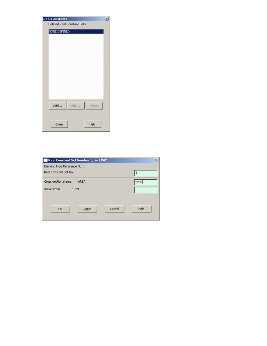
In the Preprocessor menu, select Real Constants > Add/Edit/Delete
University of Alberta ANSYS Tutorials - www.mece.ualberta.ca/tutorials/ansys/BT/Truss/Truss.html
Copyright © 2002 University of Alberta
{
Click Add... and select 'Type 1 LINK1' (actually it is already selected). Click on 'OK'. The
following window will appear:
{
As shown in the window above, enter the cross-sectional area (3250mm):
{
Click on 'OK'.
{
'Set 1' now appears in the dialog box. Click on 'Close' in the 'Real Constants' window.
6. Element Material Properties
You then need to specify material properties:
{
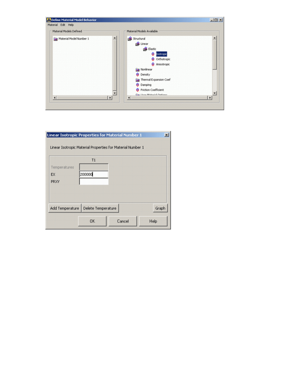
In the 'Preprocessor' menu select Material Props > Material Models
University of Alberta ANSYS Tutorials - www.mece.ualberta.ca/tutorials/ansys/BT/Truss/Truss.html
Copyright © 2002 University of Alberta
{
Double click on Structural > Linear > Elastic > Isotropic
We are going to give the properties of Steel. Enter the following field:
{
Set these properties and click on 'OK'. Note: You may obtain the note 'PRXY will be set to 0.0'.
This is poisson's ratio and is not required for this element type. Click 'OK' on the window to
continue. Close the "Define Material Model Behavior" by clicking on the 'X' box in the upper right
hand corner.
7. Mesh Size
The last step before meshing is to tell ANSYS what size the elements should be. There are a variety of
ways to do this but we will just deal with one method for now.
{
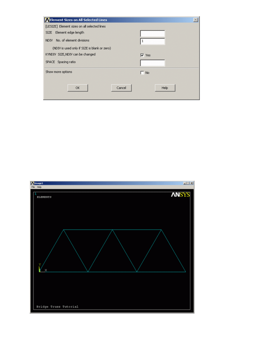
In the Preprocessor menu select Meshing > Size Cntrls > ManualSize > Lines > All Lines
EX 200000
University of Alberta ANSYS Tutorials - www.mece.ualberta.ca/tutorials/ansys/BT/Truss/Truss.html
Copyright © 2002 University of Alberta
{
In the size 'NDIV' field, enter the desired number of divisions per line. For this example we want
only 1 division per line, therefore, enter '1' and then click 'OK'. Note that we have not yet meshed
the geometry, we have simply defined the element sizes.
8. Mesh
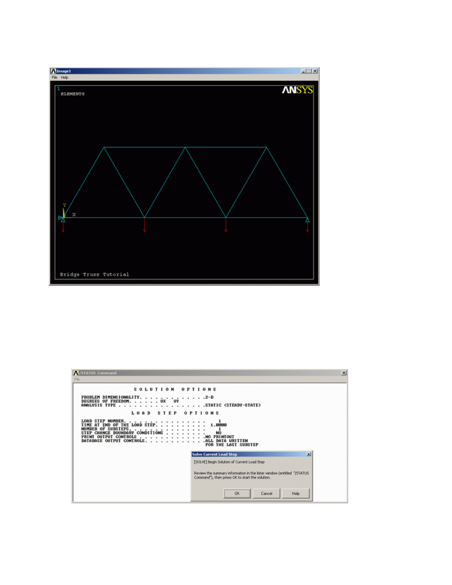
Now the frame can be meshed.
{
In the 'Preprocessor' menu select Meshing > Mesh > Lines and click 'Pick All' in the 'Mesh Lines'
Window
Your model should now appear as shown in the following window
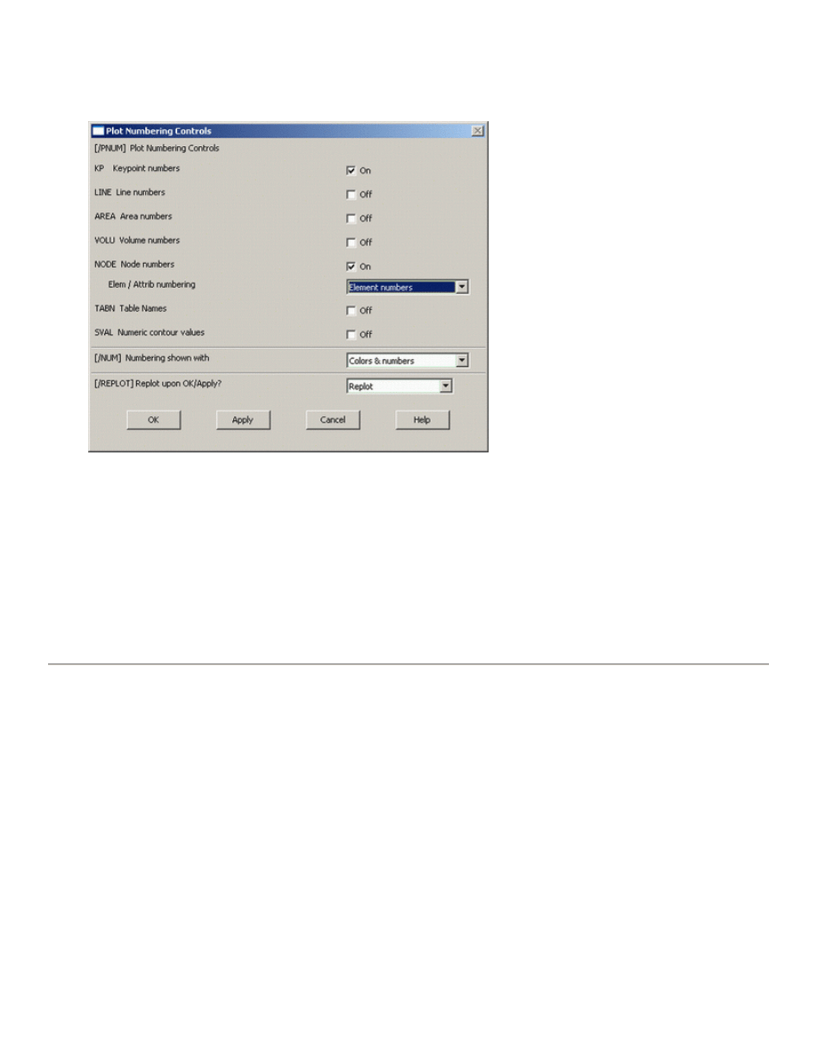
Plot Numbering
To show the line numbers, keypoint numbers, node numbers...
University of Alberta ANSYS Tutorials - www.mece.ualberta.ca/tutorials/ansys/BT/Truss/Truss.html
Copyright © 2002 University of Alberta
z
From the Utility Menu (top of screen) select PlotCtrls > Numbering...
z
Fill in the Window as shown below and click 'OK'
Now you can turn numbering on or off at your discretion
Saving Your Work
Save the model at this time, so if you make some mistakes later on, you will at least be able to come back to this
point. To do this, on the Utility Menu select File > Save as.... Select the name and location where you want to
save your file.
It is a good idea to save your job at different times throughout the building and analysis of the model to backup
your work in case of a system crash or what have you.
Solution Phase: Assigning Loads and Solving
You have now defined your model. It is now time to apply the load(s) and constraint(s) and solve the the
resulting system of equations.
Open up the 'Solution' menu (from the same 'ANSYS Main Menu').
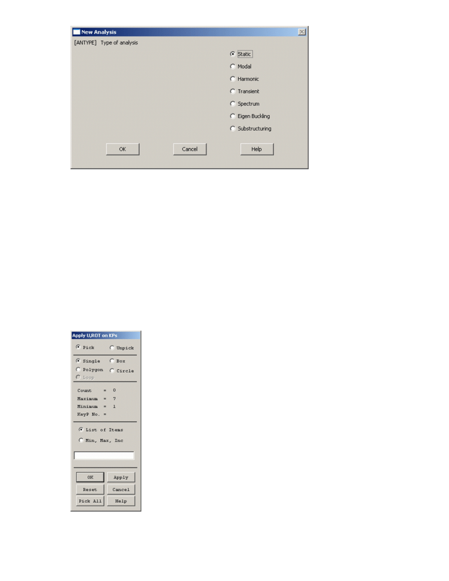
1. Define Analysis Type
First you must tell ANSYS how you want it to solve this problem:
{
From the Solution Menu, select Analysis Type > New Analysis.
University of Alberta ANSYS Tutorials - www.mece.ualberta.ca/tutorials/ansys/BT/Truss/Truss.html
Copyright © 2002 University of Alberta
{
Ensure that 'Static' is selected; i.e. you are going to do a static analysis on the truss as opposed to a
dynamic analysis, for example.
{
Click 'OK'.
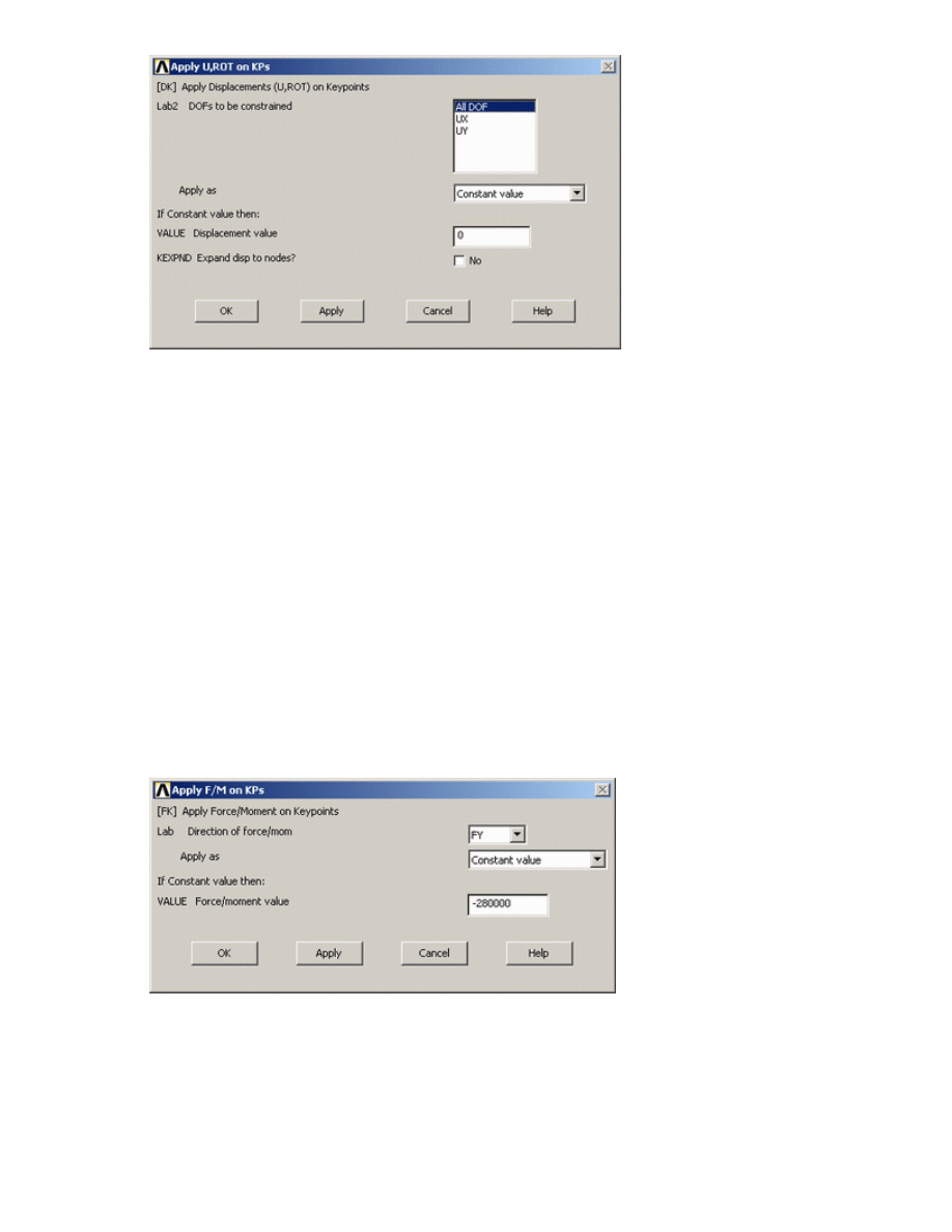
2. Apply Constraints
It is necessary to apply constraints to the model otherwise the model is not tied down or grounded and a
singular solution will result. In mechanical structures, these constraints will typically be fixed, pinned and
roller-type connections. As shown above, the left end of the truss bridge is pinned while the right end has
a roller connection.
{
In the Solution menu, select Define Loads > Apply > Structural > Displacement > On
Keypoints
{
Select the left end of the bridge (Keypoint 1) by clicking on it in the Graphics Window and click on
'OK' in the 'Apply U,ROT on KPs' window.
University of Alberta ANSYS Tutorials - www.mece.ualberta.ca/tutorials/ansys/BT/Truss/Truss.html
Copyright © 2002 University of Alberta
{
This location is fixed which means that all translational and rotational degrees of freedom (DOFs)
are constrained. Therefore, select 'All DOF' by clicking on it and enter '0' in the Value field and
click 'OK'.
You will see some blue triangles in the graphics window indicating the displacement contraints.
{
Using the same method, apply the roller connection to the right end (UY constrained). Note that
more than one DOF constraint can be selected at a time in the "Apply U,ROT on KPs" window.
Therefore, you may need to 'deselect' the 'All DOF' option to select just the 'UY' option.
3. Apply Loads
As shown in the diagram, there are four downward loads of 280kN, 210kN, 280kN, and 360kN at
keypoints 1, 3, 5, and 7 respectively.
{
Select Define Loads > Apply > Structural > Force/Moment > on Keypoints.
{
Select the first Keypoint (left end of the truss) and click 'OK' in the 'Apply F/M on KPs' window.
{
Select FY in the 'Direction of force/mom'. This indicate that we will be applying the load in the 'y'
direction
{
Enter a value of -280000 in the 'Force/moment value' box and click 'OK'. Note that we are using
units of N here, this is consistent with the previous values input.
{
The force will appear in the graphics window as a red arrow.
University of Alberta ANSYS Tutorials - www.mece.ualberta.ca/tutorials/ansys/BT/Truss/Truss.html
Copyright © 2002 University of Alberta
{
Apply the remaining loads in the same manner.
The applied loads and constraints should now appear as shown below.
4. Solving the System
We now tell ANSYS to find the solution:
{
In the 'Solution' menu select Solve > Current LS. This indicates that we desire the solution under
the current Load Step (LS).
{
The above windows will appear. Ensure that your solution options are the same as shown above
and click 'OK'.
{
Once the solution is done the following window will pop up. Click 'Close' and close the /STATUS
University of Alberta ANSYS Tutorials - www.mece.ualberta.ca/tutorials/ansys/BT/Truss/Truss.html
Copyright © 2002 University of Alberta
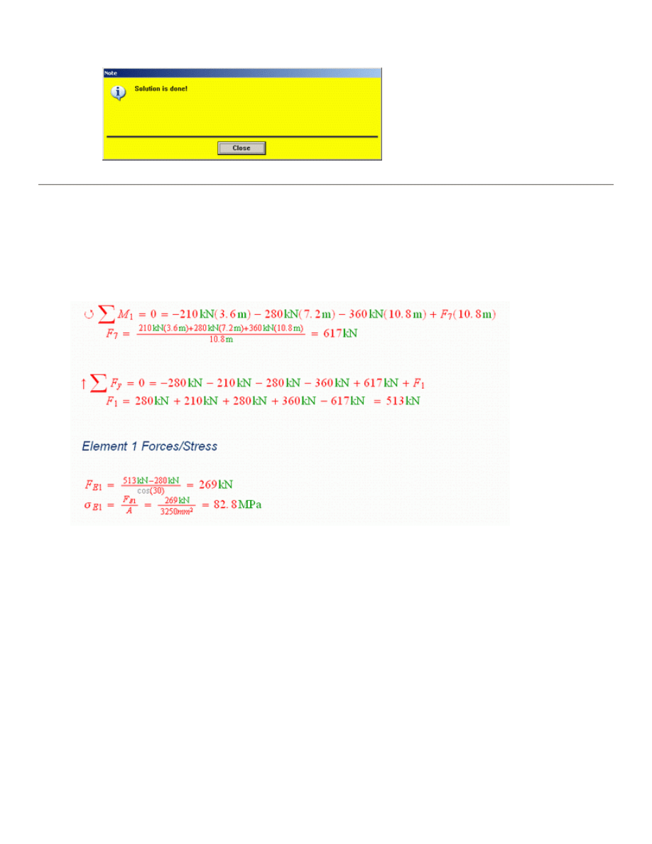
Command Window..
Postprocessing: Viewing the Results
1. Hand Calculations
We will first calculate the forces and stress in element 1 (as labeled in the problem description).
2. Results Using ANSYS
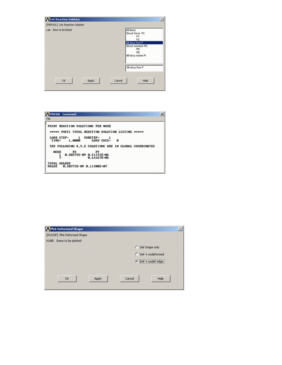
Reaction Forces
A list of the resulting reaction forces can be obtained for this element
{
from the Main Menu select General Postproc > List Results > Reaction Solu.
University of Alberta ANSYS Tutorials - www.mece.ualberta.ca/tutorials/ansys/BT/Truss/Truss.html
Copyright © 2002 University of Alberta
{
Select 'All struc forc F' as shown above and click 'OK'
These values agree with the reaction forces claculated by hand above.
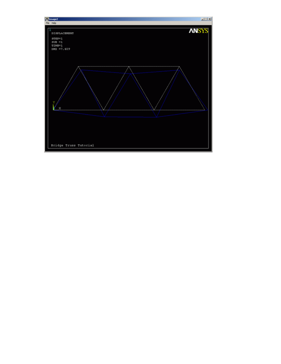
Deformation
{
In the General Postproc menu, select Plot Results > Deformed Shape. The following window will
appear.
{
Select 'Def + undef edge' and click 'OK' to view both the deformed and the undeformed object.
University of Alberta ANSYS Tutorials - www.mece.ualberta.ca/tutorials/ansys/BT/Truss/Truss.html
Copyright © 2002 University of Alberta
{
Observe the value of the maximum deflection in the upper left hand corner (DMX=7.409). One
should also observe that the constrained degrees of freedom appear to have a deflection of 0 (as
expected!)
Deflection
For a more detailed version of the deflection of the beam,
{
From the 'General Postproc' menu select Plot results > Contour Plot > Nodal Solution. The
following window will appear.
University of Alberta ANSYS Tutorials - www.mece.ualberta.ca/tutorials/ansys/BT/Truss/Truss.html
Copyright © 2002 University of Alberta
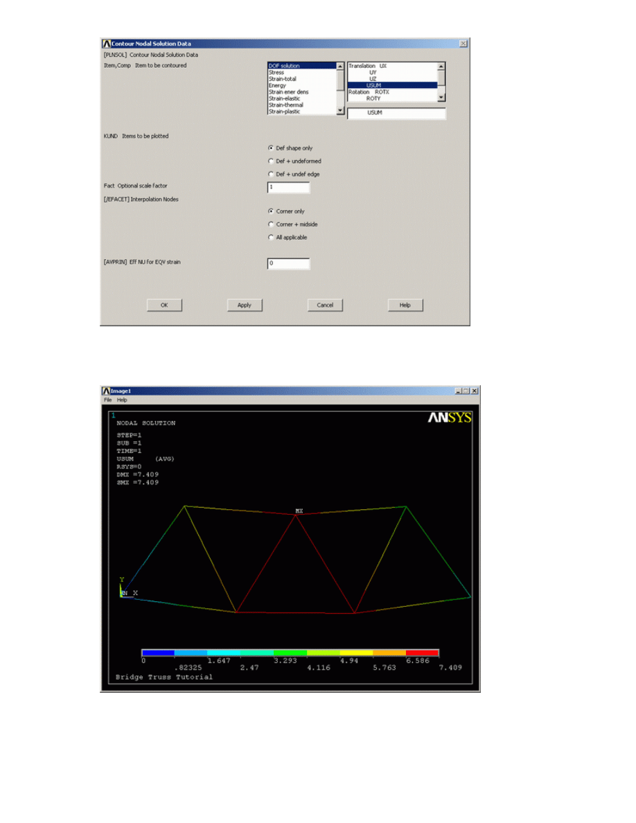
{
Select 'DOF solution' and 'USUM' as shown in the above window. Leave the other selections as the
default values. Click 'OK'.
{
Looking at the scale, you may want to use more useful intervals. From the Utility Menu select Plot
Controls > Style > Contours > Uniform Contours...
{
Fill in the following window as shown and click 'OK'.
University of Alberta ANSYS Tutorials - www.mece.ualberta.ca/tutorials/ansys/BT/Truss/Truss.html
Copyright © 2002 University of Alberta
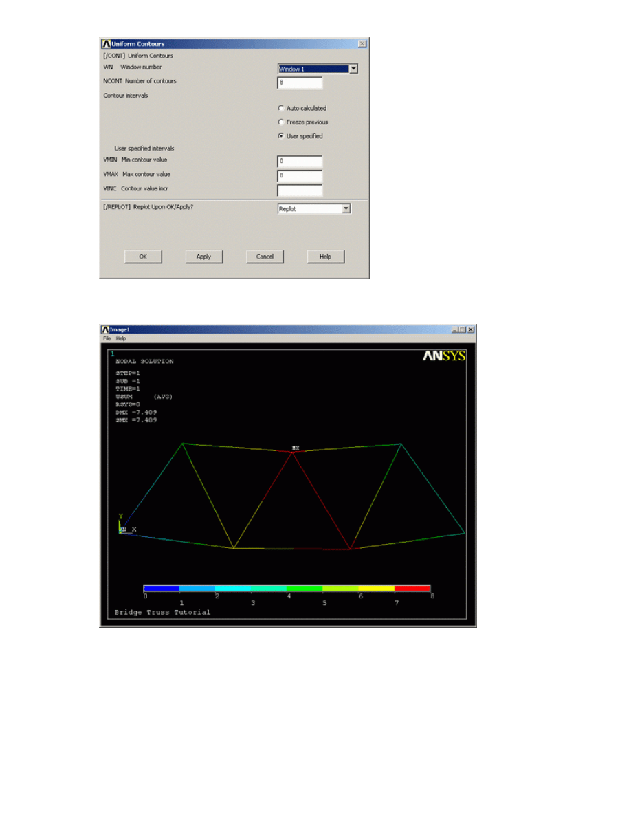
You should obtain the following.
{
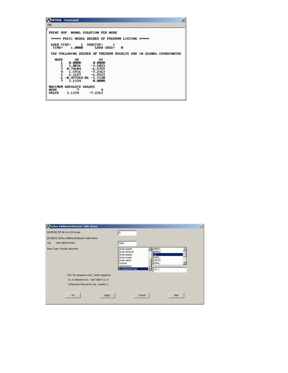
The deflection can also be obtained as a list as shown below. General Postproc > List Results >
Nodal Solution select 'DOF Solution' and 'ALL DOFs' from the lists in the 'List Nodal Solution'
window and click 'OK'. This means that we want to see a listing of all degrees of freedom from the
solution.
University of Alberta ANSYS Tutorials - www.mece.ualberta.ca/tutorials/ansys/BT/Truss/Truss.html
Copyright © 2002 University of Alberta
{
Are these results what you expected? Note that all the degrees of freedom were constrained to zero
at node 1, while UY was constrained to zero at node 7.
{
If you wanted to save these results to a file, select 'File' within the results window (at the upper left-
hand corner of this list window) and select 'Save as'.
Axial Stress
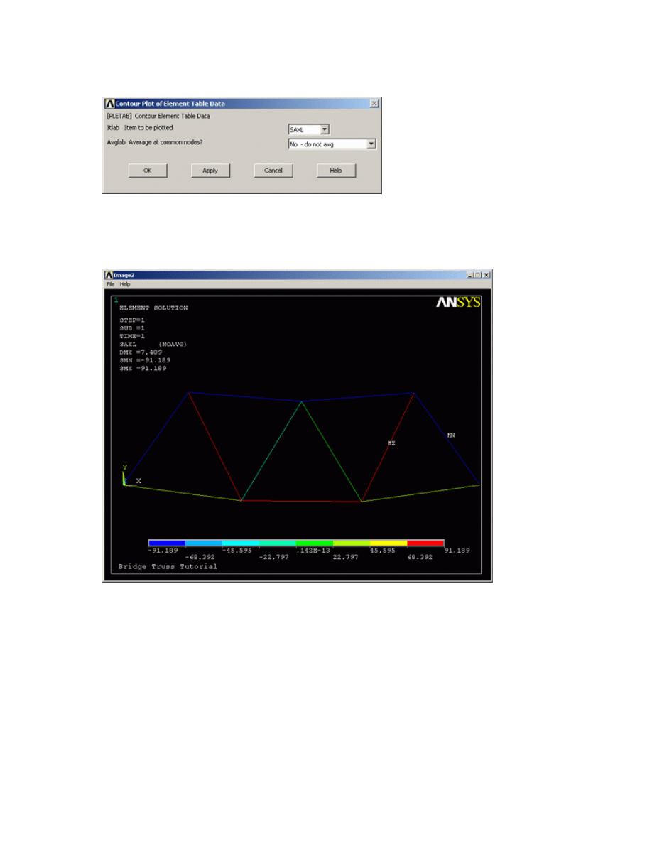
For line elements (ie links, beams, spars, and pipes) you will often need to use the Element Table to gain
access to derived data (ie stresses, strains). For this example we should obtain axial stress to compare
with the hand calculations. The Element Table is different for each element, therefore, we need to look at
the help file for LINK1 (Type
help link1
into the Input Line). From Table 1.2 in the Help file, we can
see that SAXL can be obtained through the ETABLE, using the item 'LS,1'
{
From the General Postprocessor menu select Element Table > Define Table
{
Click on 'Add...'
{
As shown above, enter 'SAXL' in the 'Lab' box. This specifies the name of the item you are
defining. Next, in the 'Item,Comp' boxes, select 'By sequence number' and 'LS,'. Then enter 1 after
LS, in the selection box
{
Click on 'OK' and close the 'Element Table Data' window.
University of Alberta ANSYS Tutorials - www.mece.ualberta.ca/tutorials/ansys/BT/Truss/Truss.html
Copyright © 2002 University of Alberta
{
Plot the Stresses by selecting Element Table > Plot Elem Table
{
The following window will appear. Ensure that 'SAXL' is selected and click 'OK'
{
Because you changed the contour intervals for the Displacement plot to "User Specified" - you
need to switch this back to "Auto calculated" to obtain new values for VMIN/VMAX.
Utility Menu > PlotCtrls > Style > Contours > Uniform Contours ...
Again, you may wish to select more appropriate intervals for the contour plot
{
List the Stresses
From the 'Element Table' menu, select 'List Elem Table'
From the 'List Element Table Data' window which appears ensure 'SAXL' is highlighted
Click 'OK'
University of Alberta ANSYS Tutorials - www.mece.ualberta.ca/tutorials/ansys/BT/Truss/Truss.html
Copyright © 2002 University of Alberta
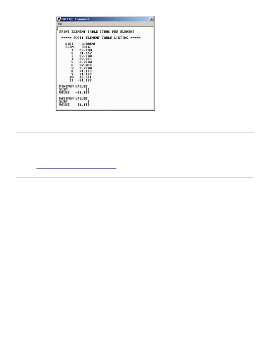
Note that the axial stress in Element 1 is 82.9MPa as predicted analytically.
Command File Mode of Solution
The above example was solved using the Graphical User Interface (or GUI). This problem has also been solved
using the
ANSYS command language interface
that you may want to browse. Open the file and save it to your
computer. Now go to 'File > Read input from...' and select the file.
Quitting ANSYS
To quit ANSYS, select 'QUIT' from the ANSYS Toolbar or select Utility Menu/File/Exit.... In the dialog box
that appears, click on 'Save Everything' (assuming that you want to) and then click on 'OK'.
University of Alberta ANSYS Tutorials - www.mece.ualberta.ca/tutorials/ansys/BT/Truss/Truss.html
Copyright © 2002 University of Alberta
Wyszukiwarka
Podobne podstrony:
1 Two Dimensional Truss
Evaporation of Two Dimensional Black Holes
Maffra, Gattass Propagation of Sound in Two Dimensional Virtual Acoustic Environments
44 611 624 Behaviour of Two New Steels Regarding Dimensional Changes
All Flesh Must Be Eaten Two Rotted Thumbs Up
P000476 D Eng Main dimensions
Brit M Two Men and a Lady Prequel [Ravenous] (pdf)
550 Dimensions35175
Mastercam creating 2 dimensio Nieznany
In literary studies literary translation is a term of two meanings rev ag
Day Two Creating Instant Confidence
Dimensioning
DIMENSIONS OF INTEGRATION MIGRANT YOUTH IN POLAND
[Strizenec] DIMENSIONS OF SPIRITUALITY [paper]
2 bedroom two storey house T shaped
worksheet two
Existence of the detonation cellular structure in two phase hybrid mixtures
A Comparison of two Poems?out Soldiers Leaving Britain
więcej podobnych podstron