Propagation of Sound in Two-Dimensional Virtual Acoustic Environments

S ´

ERGIO

A

LVARES

R.

DE

S. M

AFFRA

1

, M

ARCELO

G

ATTASS

1

, L

UIZ

H

ENRIQUE DE

F

IGUEIREDO

2

1

Tecgraf/PUC-Rio – Rua Marquˆes de S˜ao Vicente, 225, 22453-900, Rio de Janeiro, RJ, Brasil

{

sam,gattass

}

@tecgraf.puc-rio.br

2

IMPA – Instituto de Matem´atica Pura e Aplicada - Estrada Dona Castorina, 110, 22460-320, Rio de Janeiro, RJ, Brasil

[e-mail]

Abstract.

This paper describes the implementation of a system that simulates the propagation of sound in

two-dimensional virtual environments and is also capable of reproducing audio according to this simulation. The
simulation, which is a preprocessing stage, consists in creating direct, specular reflection and diffraction sound
beams that are used later for the creation of the actual propagation paths, in real-time. As the sound beams are
created in a preprocessing stage, the system treats only sound sources with fixed position and moving receivers.

1

Introduction

For a long time, the computational simulation of acoustic
phenomena has been used mainly in the design and study
of the acoustic properties of concert and lecture halls. Re-
cently, however, there has been a growing interest in the
use of such simulations in virtual environments in order to
enhance users’ immersion experience. The addition of re-
alistic simulation of acoustic phenomena to a virtual real-
ity system can, according to Funkhouser et al. [1], aid in
the localization of objects, in the separation of simultane-
ous sound events and in the spatial comprehension of the
environment.

Generally, we can say that a virtual acoustic environ-

ment must be able to accomplish two tasks: simulating the
propagation of sound in an environment and reproducing
audio with spatial content, that is, in a way that allows
its user to recognize the direction of the incoming sound
waves.

To simulate the propagation of sound, one can solve

the wave equation [2] using finite and boundary element
methods [3]. This approach, however, is not suitable for
interactive applications due to its high computational cost.
An alternative to these expensive methods is the geometric
treatment of the propagation of sound, referred to as geo-
metrical room acoustics [4]. As Kuttruff describes it, in
geometrical room acoustics the concept of a sound wave is
replaced by the concept of a sound ray.

The use of sound rays to simulate the propagation of

sound in an environment makes the algorithms created for
this purpose very similar to the ones used in the analysis
of wireless communication networks [5] and in visualiza-
tion (hidden surface removal), such as ray tracing [6] and
beam tracing [7]. This means that the same techniques
used to speed up visualization applications can also be used
in the simulation of sound propagation, as was shown by

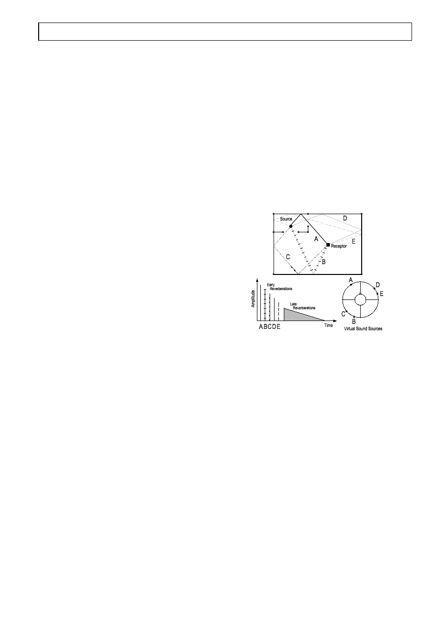
Figure 1: Propagation paths and virtual sound sources

Funkhouser et al.[1].

The reproduction of the simulated sound field is made

by superposing several virtual sound sources located around
the user. For each propagation path found between the
sound source being simulated and the receptor, a virtual
sound source is created. The position and volume of a vir-
tual source are defined (as described in Section 4) by the
properties of its corresponding propagation path (length, re-
flections, etc).

Figure 1 illustrates how a virtual acoustic environment

works. The figure contains the drawing of a simple envi-
ronment, composed of two rooms. First, propagation paths
between the sound source and the receptor are computed.
In the figure, five propagation paths were found (labeled A
to E). These propagation paths are then used to create the
virtual sound sources around the receptor. These can be
seen on the lower right corner of the figure. Each virtual

II Workshop de Teses e Dissertações em Computação Gráfica e Processamento de Imagens

source received the label of its corresponding propagation
path. Notice how they are positioned around the user ac-
cording to angle of incidence of the paths at the receptor.
The chart on the lower left corner indicates the time delay
of each propagation path.

2

Previous Work

The work of Funkhouser et al. [1, 8] address the construc-
tion of propagation paths, comprised of direct incidences
and specular reflections, in three-dimensional environments
using a beam tracing technique. Their first work [1] dealt
only with fixed sound sources but, by using a distributed
processing architecture and a few modifications in their orig-
inal algorithm, they were able to extend it to treat moving
sound sources [8] in real-time. Tsingos et al. [9] then ex-
tended the fixed source algorithm by adding diffraction to
the propagation paths.

In our work we implemented a beam tracer capable

of creating beams of specular reflection and diffraction in
two-dimensional environments. Two reasons motivated us
into restricting our system to the two-dimensional case. The
first is the simplification of data structures and operations
required to implement the algorithm, which results in an al-
gorithm that, when compared to the 3D case, is easier to im-
plement, more efficient and that requires less memory. The
second reason is the fact that 2D propagation paths can still
be usefull. It is possible, for example, to unproject these 2D
paths in order to treat 2.5D environments (environments de-
fined by the vertical sweeping of 2D shapes) [10]. Also, for
applications that do not require a rigorous acoustic simula-
tion, like computer games, the tracing of 2D paths can be a
good approximation.

As original contributions, we present an approximate

and more efficient formula to evaluate the contribution of
a propagation path to a sound field (Section 3.3.3) and a
new method to create the cellular decomposition of a two-
dimensional environment (Section 3.4).

3

Propagation of sound

There are three basic methods that can be used to enumer-
ate propagation paths comprised of specular reflection and
diffraction. Namely, the virtual source method [4], ray trac-
ing [6] and beam tracing [1].

The virtual source method is basically an exhaustive

enumeration technique. Its main problem is computational
effort wasted in the generation of a large number of invalid
paths, which must be identified and discarded. These in-
valid paths are created due to the lack of visibility informa-
tion in the method.

Ray tracing has a well known discretization (aliasing)

problem: no matter how close rays from the same source
are created near their origin, as their distance to the source

increases, so does the gap between neighboring rays. The
existence of gaps between rays creates discontinuities in the
sound field that can lead to audible artifacts.

Beam tracing algorithms fix the problems of the pre-

vious methods by dealing with beams, represented by a re-
gion of space, instead of individual rays and by using visi-
bility information in the creation of beams, as we show on
the next sections. The disadvantage of the beam tracing
technique is the complexity of the geometric primitives and
data structures necessary for its implementation.

3.1

Beam representation

We begin our brief explanation of the beam tracing method
by describing the representation of beams. As we men-
tioned before, beams are represented by a region of space.
This means that a single beam can represent an infinite
number of rays, which eliminates the aliasing that occur in
ray tracing.

In our implementation, we have used the same repre-

sentation for beams used by Heckbert and Hanrahan [7],
where beams are represented by a local coordinate system
(the beam coordinate system) and by a cross-section defined
in this coordinate system, as Figure 2 illustrates. The figure
shows on the left a beam defined in the global coordinate
system (axes x and y) with its local coordinate system (axes
x

0

and y

0

). On the right it shows the same beam (now in its

local coordinate system) and its cross-section (defined by
the position of a vertical projection plane (x

p

) and an inter-

val located on this projection plane [y

pi

, y

pf

]).

The cross-section of a beam is responsible for limiting

the area it occupies. Notice, however, that beams are actu-
ally structures with infinite area, as the cross-section only
limits how open beams are and not how far they can reach.
That is, rays defined inside the gray area shown in Figure 2
have infinite length.

An essential part of the beam tracing method, as im-

plemented in our system, is the decomposition of the en-
vironment into convex cells. This decomposition permits
the efficient traversal of the environment and also allows to
limit the range of a beam, as each beam must be associ-
ated with a single cell of the environment. This association
means that operations realized with a beam are valid only
inside the cell it is associated with. The next section defines
the basic operations that are performed on beams.

Figure 3 illustrates the association between beams and

convex cells. Notice that two different beams are created
when the original beam (a) strikes the boundary of the first
cell. Beam c is a reflection beam, created due to the inter-
section of beam a with an opaque portion of the boundary
of the cell. The intersection of the original beam with a
transparent portion of the boundary originates a transmis-
sion beam (beam b), that only differs from the original beam

Figure 2: Representation of beams

in its cross-section.

3.2

Beam operations

There are two basic operations that are frequently made
on beams during a beam tracing algorithm: determining
whether a beam contains a point in space and determining
the intersection of a beam and a segment of the boundary
of a convex cell of the environment. Both operations are
based on the projection of a vertex in the cross-section of a
beam. This projection is made along the ray defined (in the
beam coordinate system) by the origin of the beam and the
vertex.

Once the projection is made, it is enough to check if

the projected vertex lies inside the interval that limits the
cross-section to determine if the vertex being tested is lo-
cated inside the beam.

The intersection of a beam and a segment of the en-

vironment is used in the creation of transmission and re-
flection beams to determine the cross-section of the new
beams. When the newly created beams inherit the posi-
tion of the projection plane from the beam that originated
them, the intersection operation can be greatly simplified.
In this case, the only information needed for the creation of
the new beams is the interval that results from the intersec-
tion of two other intervals: the cross-section of the original
beam and the interval defined by the projection of the end-
points of the segment in the projection plane of the original
beam.

For more detail on the implementation of the basic op-

erations performed with beams, in two and three dimen-
sions, refer to the full text [11].

3.3

Beam tracing

The beam tracing method has two stages. The first stage,
implemented in our system as preprocessing stage, com-
prises the construction of the beam-tree data structure. The
beam-tree is the data structure that links all beams origi-
nating from the same source, allowing the construction of
the actual propagation paths, which is the second stage of
the method. Each node of a beam-tree represents a beam

Figure 3: Beams and their association to cells

that is linked to its parent beam (the one responsible for its
creation). Figure 3 illustrates the beam-tree created for the
beams illustrated in the figure and the association of beams
and convex cells. The next sections discuss the stages of the
beam tracing method in more detail and also how the con-
tribution of each propagation path for the simulated sound
field is calculated.

3.3.1

Beam-tree construction

As mentioned in the previous sections, whenever a beam
intersects a segment of the environment a new beam is cre-
ated. This creation involves the computation of the new
beam’s representation (local coordinate system and cross-
section), its insertion in the beam-tree and its association to
one of the convex cells of the environment.

The segments intersected by the beams can be either

opaque (represented in our figures as continuous line seg-
ments) or transparent (represented as dashed line segments).
Opaque segments represent the walls of the environment
that reflect sound waves, while transparent segments are ar-
tificial walls, commonly referred to as portals [12], that are
inserted in the environment to obtain its convex cell decom-
position.

When an opaque segment is intersected, a new reflec-

tion beam is created. Its coordinate system can be obtained
by reflecting the coordinate system on the line supporting
the segment. The cross-section of the new beam can be ob-
tained by performing the intersection of the original beam
with the segment (as described in Section 3.2). Finally,
reflection beams are always associated with the same cell
associated with its parent beam. In the case of an inter-
section with a transparent segment, the new beam inherits
the coordinate system of its parent and is associated with a
neighboring cell (the one adjacent through the intersected
segment). As with opaque segments, the cross-section of
the new beam is obtained by the intersection with the par-
ent beam.

There is also another kind of beam we have neglected

to mention until now: diffraction beams. Diffraction is the
scattering of a wave that happens when it strikes a wedge
of the environment. Figure 4 illustrates the diffraction of a
wave incident to a wedge. Notice how the scattered wave
propagates in all directions around the wedge, forming the

Figure 4: Diffraction beams

figure of a cone. As the scattered wave propagates in all
directions around the wedge, the number of beams might
explode. To avoid this increase in the number of beams we
use the same approximation adopted by Tsingos et al. [13]:
diffraction beams are traced only in the shadow region of
the wedge (the region around the wedge that is not illumi-
nated by the incident beam). This approximation is also
shown in Figure 4. The justification for using diffraction
beams that only cover the shadow region is the high at-
tenuation of the amplitude of the wave caused by diffrac-
tion. In the region around the wedge that is illuminated by
the incident wave and, occasionally, by its reflection, the
contribution of the scattered wave can be discarded without
great losses to the resulting sound field. Notice that in the
shadow region, the only contribution to the sound field is
the diffracted wave, which explains why its contribution is
accounted for.

In the beam tracing algorithm, a new diffraction beam

must be created whenever a beam intersects a wedge of the
environment, which happens when it intersects two consec-
utive segments, one opaque and the other transparent.

Regarding the construction of beam-trees, there is only

one more consideration: the termination criteria for the con-
struction of the tree. The most natural criterium for termi-
nating the expansion of a branch of the beam-tree is an audi-
tive criterium, that is, beams should not be created when the
sound becomes inaudible. Limiting the maximum number
of beams created and the maximum number of reflections
and diffractions in each branch are also commonly used.

3.3.2

Propagation path construction

The second stage of the beam tracing method is the one
executed in real-time and is responsible for the creation of
the actual propagation paths between the sound source and
the receiver. As we mentioned before, each beam stored
in the beam-tree contains a reference to its parent beam.
Therefore, given any beam b, it is possible to traverse the
beam-tree, passing through all ancestor beams of b until the
sound source is reached. It is by making this traversal that
one can build an actual propagation path between a source
and a receiver.

In order to create the propagation paths, the position

Figure 5: Constructing propagation paths on a beam-tree

occupied by the receiver must be determined (which is un-
determined during the construction of the beam-tree). Once
its position is known, to create the propagation paths the
beams that contain the receiver must be identified. This
identification can be performed quite efficiently by examin-
ing all the beams associated with the convex cell that con-
tains the receiver. Notice that for each beam that contains
the receiver, a different propagation path can be built, as for
each beam there is a different path on the beam-tree that
leads to the source.

The construction of a propagation path is illustrated in

Figure 5. The figure shows a rectangular environment with
three different beams and the resulting beam-tree. Since
the beam c contains the receiver, it is the starting point of
the path towards the sound source. Also, note that each
node along this path contributes with a segment to the prop-
agation path (the intermediary propagation paths are shown
next to the arrows that indicate the path along the beam-
tree).

3.3.3

Attenuation and delay

Once the propagation paths have been found, the contribu-
tion of each path to the resulting sound field must be calcu-
lated. Because our main interest is not the rigorous analysis
of acoustic phenomena, we have adopted several simplifi-
cations in the computation of the contribution of each prop-
agation path.

As Funkhouser et al. [1], we disregard phase informa-

tion when computing the amplitude of the wave reaching
the receiver and the phase change due to reflections, that
is modelled as a frequency independent constant factor (α
in the expression below). Phase changes due to diffraction
are also ignored. Given the complexity of the evaluation
of more rigorous formulations for diffraction, such as the
Uniform Geometrical Theory of Diffraction [14] or the Di-
rective Line Source Method [15], we have adopted an ap-

proximation (δ(θ), defined in the formulas below) that we
believe captures the essence of the effects caused by diffrac-
tion, that is the growing attenuation suffered by the ampli-
tude of the scattered wave as it goes deeper into the shadow
region around a diffracting wedge. This approximation was
obtained through a curve-fitting approach, using diffraction
charts presented by Tsingos et al. [13].

The formula below contains the expression used to

compute the amplitude of the wave at the receiver. The
propagation path modelled in the formula has suffered r re-
flections, d diffractions and has length l. P

0

is the initial

amplitude of the wave. The diffraction attenuation term of
the formula receives as parameter an angle θ that measures
how deep into the shadow region the propagation path is.

P = P

0

α

r

Q

d
i=1

δ(θ

i

)

l

δ(θ) =

1

1 + Kθ

n

K = 130

n = 1.66

The time delay associated with a propagation path is

given by l/c, where c is the velocity of propagation of sound.

For a more detailed explanation on the calculation of

the attenuation and delay suffered by a sound wave, refer to
the full text [11].

3.4

Cell partitioning of the environment

As stated previously, the decomposition of the environment
into convex cells is an essential part of the beam tracing al-
gorithm. It simplifies the representation of beams, which
can be modelled as infinite areas. It also defines an or-
der among the occluders of the environment allowing the
implementation of efficient visibility queries and efficient
traversal of the environment, which are essential for the ef-
ficient creation of beams [11].

The decomposition of an environment into convex cells

is usually made using binary space partitions (BSP) [1, 8,
16, 13, 12]. The disadvantage of this technique is the occa-
sional generation of decompositions with a large number of
cells. When a large number of cells is created unnecessar-
ily, the large number of portals (or transparent segments) in
the decomposition can cause a large increase in the number
of beams traced, since whenever a beam crosses a portal, a
new transmission beam is created [11].

To avoid this increase in the number of beams traced,

we have developed a new method, by modifying the tech-
nique used by Teller [12] to create cellular decompositions
of two-dimensional environments. Teller’s technique con-
sists in using a Constrained Delaunay Triangulation [17]
algorithm to obtain the decomposition. The triangulation,

a) Input environment

b) BSP partitioning

c) Removal of edges in decreasing length order

Partitioning

Cells

Vertices

Occluders

Portals

a

–

380

378

0

b

584

883

851

615

c

206

380

378

207

Figure 6: Comparison of cell partitioning methods

however, also has a large number of cells, not solving the
problem of the unnecessary increase in the number of beams.
We have avoided this problem by removing edges of the tri-
angulation. Once the triangulation is built, its transparent
edges (portals) are sorted in decreasing length order and
then removed from the triangulation once it is determined
that its removal will not create a concave cell in the decom-
position [11].

Figure 6 illustrates the results obtained by the tech-

niques described in the section when applied to the model
of a real residential building. As the figure illustrates, the
result obtained in this example by the simplification of a tri-
angulation is much superior to the one obtained by the BSP
technique.

4

Auralization

Auralization is a term created to describe the rendering of

Figure 7: A few propagation paths computed for the resi-
dencial building example

sound fields, in analogy to visualization. Many systems for
the auralization of sound fields have been developed along
the years. A good overview of such systems and of how the
localization of sound sources by human beings occur can be
found in the course notes created by Funkhouser et al. [18]
and in the full text [11].

The rendering of the simulated sound field is accom-

plished by using several virtual sound sources. Being a
somewhat lengthy subject, we leave the description on how
such virtual sources are implemented to the references above.

The creation of these virtual sound sources was dele-

gated to the DirectX library [19], which offers several algo-
rithms that implement virtual sound sources and also sup-
ports different reproduction systems, like headphones and
several arrangements of loudspeakers.

To auralize the simulated sound field, we create a dif-

ferent sound source for each propagation path found be-
tween the source and the receiver. The position of these
sound sources is determined, as in a polar coordinate sys-
tem, by the length of the propagation path and the incidence
angle of the wave at the receiver (which is determined by
the last segment of the propagation path). The attenuations
due to the reflections and diffractions suffered by the wave
along a propagation path were simulated by adjusting the
volume of the virtual sound source.

We used a 5.1 surround sound system [20] and head-

phones as our test reproduction systems.

5

Results

In our tests we obtained the same qualitative results ob-
tained in the literature, such as an exponential growth in
the number of traced beams with the increase of the num-
ber specular reflections in each propagation path [1] and the
acceleration of this growth [13] with the addition of diffrac-
tions. This behavior is illustrated in Figure 8, which con-
tains graphics indicating the number of beams created (and
the time spent in their creation) as a function of the num-
ber of reflections and diffractions in each propagation path
for the environment illustrated in Figure 9. Notice that, as

the attenuation of the sound wave increases with the reflec-
tions, diffractions and the length of the propagation path,
the audible propagation paths are not expected to contain
many reflections and diffractions. This means that in most
cases, the number of beams is not expected to explode. The
time results contained in Figure 8 are the result of an av-
erage of 10 experiments, performed on a Pentium 4 2 GHz
computer, with 512 MB of RAM.

We also noticed that the addition of diffraction beams

to the propagation paths results in smoother sound fields [13];
we believe that this validates the approximation used to
evaluate the attenuation of the sound wave due to diffrac-
tions. We also noticed that the addition of diffraction can
dramatically improve the coverage of the environment [11].
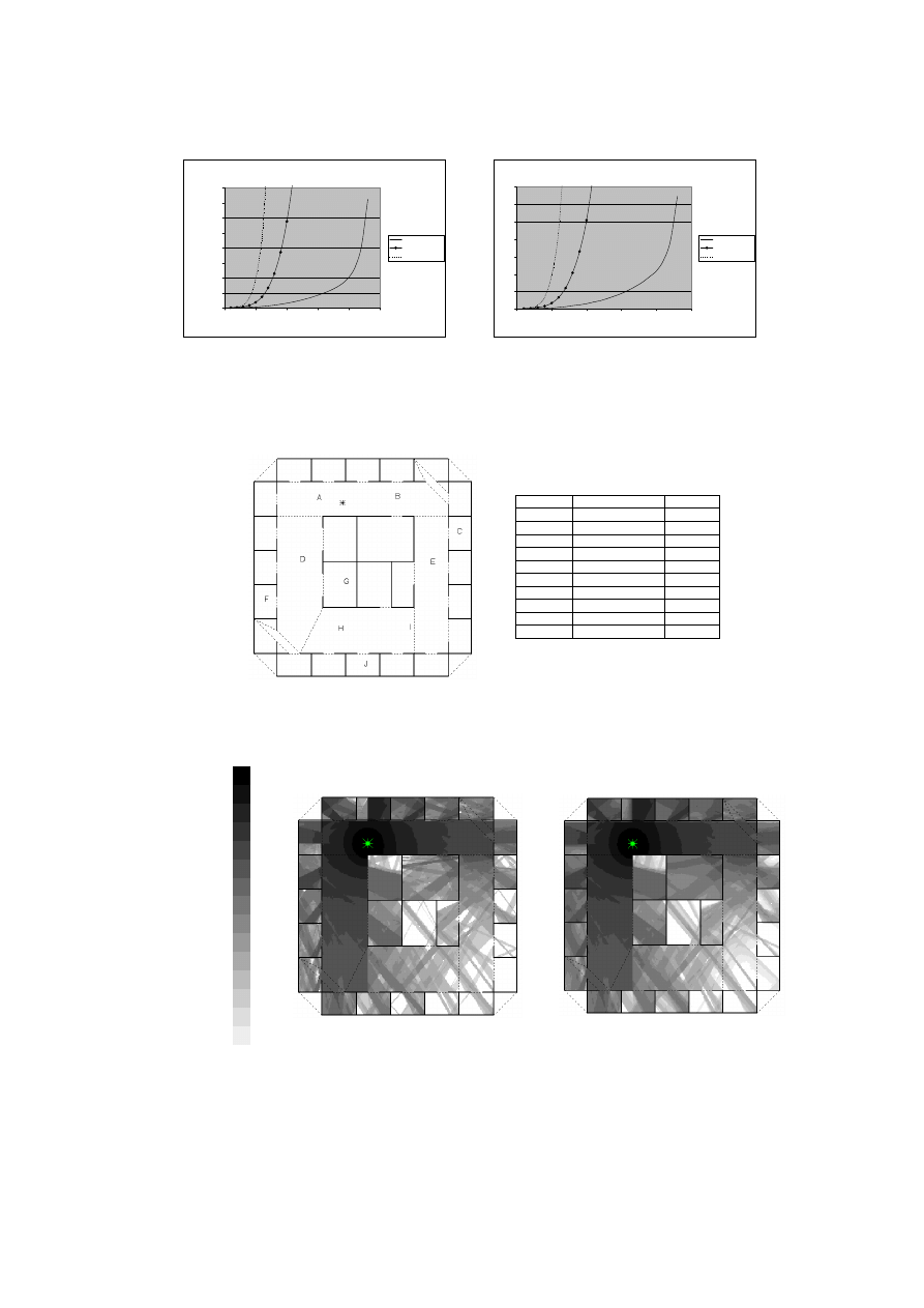
Figure 10 contains two different sound intensity level fields,
computed to illustrate the effect of diffraction. The field
without diffraction was constructed with six reflections and
the one with diffraction with five reflections and one diffrac-
tion. Notice that with diffraction, the individual beams are
more difficult to be identified, specially in the rooms near
the sound source, represented as an asterisk in the figure.

Regarding the performance of the algorithm in the sim-

ulation stage, our initial tests indicate that it is suitable for
the construction of a large number of propagation paths in
real-time. Figure 9 contains the results obtained for a test
where paths with eight reflections and 1 diffraction were
computed. Several positions were chosen in the environ-
ment to evaluate the performance of the path construction
stage. The results shown in the figure are the average of
100 experiments performed on an Athlon 1 GHz computer,
with 512 MB of RAM.

6

Conclusions and future work

The main objective when we started this work was to ob-
tain more familiarity with a subject previously unknown to
us. Given the accordance of our results to the ones existing
in the literature and the performance of the algorithm im-
plemented we believe to have successfully implemented a
simple virtual acoustic environment.

Our system can still be extended in several ways. The

transmission of sound through walls and the use of different
materials for the occluders of the environment can be eas-
ily implemented. The first can be implemented using the
same procedure used in the transmission of beams through
portals and the second consists in replacing the constant α
used in the formula that computes the attenuation of sound
by a material dependent term (Section 3.3.3). We can also
use more physically correct models to evaluate the attenu-
ation due to diffractions and reflections. Another possible
extension is the modification of the beam tracing algorithm
to treat moving sound sources, as was made by Funkhouser
et al. [8] with the use of parallel processing.

Currently, we are working on extending our system

to handle 2.5D environments [10]. We are also studying
the possibility of using our algorithm in a computer game
that is currently under development at PUC-Rio and appli-
cations of beam tracing for the propagation of radio signals.
This application can probably help determining the cover-
age of a wireless network, what could help on the design of
such networks.

Acknowledgements

We would like to PUC-Rio and CAPES for the support that
made this work possible. We would also like to thank Tec-
Graf for the resources allocated during this work.

References

[1] Thomas Funkhouser, Ingrid Carlbom, Gary Elko,

Gopal Pingali, Mohan Sondhi, and Jim West. A Beam
Tracing Approach to Acoustic Modeling for Interac-
tive Virtual Environments. In Proceedings of the 25th
annual conference on Computer graphics and inter-
active techniques, pages 21–32. ACM Press, 1998.

[2] Philip M. Morse and K. Uno Ingard.

Theoretical

Acoustics. Princeton University Press, 1986.

[3] Mendel Kleiner, Bengt-Inde Dalenb¨ack, and Peter

Svensson. Auralization – An Overview. In Journal
of the Audio Engineering Society, volume 41, pages
861–875, 1993.

[4] Heinrich Kuttruff. Room Acoustics. Spon Press, third

edition, 2000.

[5] Manuel F. Catedra and Jesus Perez. Cell Planning for

Wireless Communications. Artech House, 1999.

[6] Arthur Appel. Some techniques for shading machine

renderings of solids.

In AFIPS 1968 Spring Joint

Computer Conf., volume 32, pages 37–45, 1968.

[7] Paul S. Heckbert and Pat Hanrahan.

Beam Trac-

ing Polygonal Objects. In Hank Christiansen, editor,
Computer Graphics (SIGGRAPH ’84 Proceedings),
volume 18, pages 119–127, 1984.

[8] Thomas A. Funkhouser, Patrick Min, and Ingrid Carl-

bom. Real-Time Acoustic Modeling for Distributed
Virtual Environments.

In Alyn Rockwood, edi-

tor, Siggraph 1999, Computer Graphics Proceedings,
pages 365–374, Los Angeles, 1999. Addison Wesley
Longma.

[9] Nicolas Tsingos, Thomas Funkhouser, Addy Ngan,

and Ingrid Carlbom. Geometrical Theory of Diffrac-
tion for Modeling Acoustics in Virtual Environ-
ments.

Technical Report 10009662-000802-03TM,

Bell Labs, January 2000.

[10] S´ergio Alvares Maffra and Marcelo Gattass. Propa-

gation Paths in 2.5D Environments. In Climdiff 2003
Proceedings, 2003. Accepted for publication.

[11] S´ergio Alvares Rodrigues de Souza Maffra. Propa-

gac˜ao de som em ambientes ac´usticos virtuais bidi-
mensionais.

Master’s thesis, Departamento de In-

form´atica - Pontif´ıcia Universidade Cat´olica do Rio
de Janeiro, 2003.

[12] Seth J. Teller. Visibility Computations in Densely Oc-

cluded Polyhedral Environments. PhD thesis, Dept. of
Computer Science, University of California at Berke-
ley, 1992.

[13] Nicolas Tsingos, Thomas Funkhouser, Addy Ngan,

and Ingrid Carlbom.

Modeling Acoustics in Vir-

tual Environments Using the Uniform Theory of
Diffraction.

In Eugene Fiume, editor, SIGGRAPH

2001, Computer Graphics Proceedings, pages 545–
552, 2001.

[14] D. A. McNamara, C.W.I. Pistorius, and J. A. G. Mal-

herbe. Introduction to The Uniform Geometrical The-
ory of Diffraction. Artech House, 1990.

[15] Penelope Menounou, Ilene J. Busch-Vishniac, and

David T. Blackstock. Directive Line Source Model:
a new model for sound diffraction by half planes and
wedges. Journal of the Acoustical Society of America,
107(6):2973–2986, June 2000.

[16] Patrick Min and Thomas Funkhouser. Priority-Driven

Acoustic Modeling for Virtual Environments. Com-
puter Graphics Forum, 19(3).

[17] M. de Berg, M. van Kreveld, M. Overmars, and

O. Schwarzkopf.

Computational Geometry: Algo-

rithms and Applications. Springer Verlag, second edi-
tion, 2000.

[18] Thomas Funkhouser, Jean-Marc Jot, and Nicolas

Tsingos. Sounds Good To Me. In SIGGRAPH 2002
Course Notes, 2002.

[19] DirectX. http://www.microsoft.com/directx.

[20] Francis Rumsey. Spatial Audio. Music Technology

Series. Focal Press, 2001.

Growth of the number of beams

0

50000

100000

150000

200000

250000

300000

350000

400000

0

5

10

15

20

25

Number of Reflections

Number of Beams

No Diffraction
1 Diffraction
2 Diffraction

Time spent on the creation of beams

0

1

2

3

4

5

6

7

0

5

10

15

20

25

Number of Reflections

Time (s)

No Diffraction
1 Diffraction
2 Diffractions

Figure 8: Beam tracing performance test

Receptor

Number of Paths

Time (s)

A

414

0.012

B

478

0.012

C

117

0.003

D

338

0.013

E

303

0.010

F

174

0.005

G

199

0.005

H

159

0.006

I

143

0.005

J

40

0.001

Figure 9: Path construction performance test

91.7 a 95.0 dB

88.3 a 91.7 dB

85.0 a 88.3 dB

81.7 a 85.0 dB

78.3 a 81.7 dB

75.0 a 78.3 dB

71.7 a 75.0 dB

68.3 a 71.7 dB

65.0 a 68.3 dB

61.7 a 65.0 dB

58.3 a 61.7 dB

55.0 a 58.3 dB

51.7 a 55.0 dB

48.3 a 51.7 dB

45.0 a 48.3 dB

Figure 10: Sound intensity level fields without (left) and with (right) diffraction