
MIPS Assembly Language Programming
CS50 Discussion and Project Book
Daniel J. Ellard
September, 1994

Contents
1 Data Representation
1
1.1
Representing Integers . . . . . . . . . . . . . . . . . . . . . . . . . . .
1
1.1.1
Unsigned Binary Numbers . . . . . . . . . . . . . . . . . . . .
1
1.1.1.1
Conversion of Binary to Decimal . . . . . . . . . . .
2
1.1.1.2
Conversion of Decimal to Binary . . . . . . . . . . .
4
1.1.1.3
Addition of Unsigned Binary Numbers . . . . . . . .
4
1.1.2
Signed Binary Numbers . . . . . . . . . . . . . . . . . . . . .
6
1.1.2.1
Addition and Subtraction of Signed Binary Numbers
8
1.1.2.2
Shifting Signed Binary Numbers . . . . . . . . . . .
9
1.1.2.3
Hexadecimal Notation . . . . . . . . . . . . . . . . .
9
1.2
Representing Characters . . . . . . . . . . . . . . . . . . . . . . . . .
10
1.3
Representing Programs . . . . . . . . . . . . . . . . . . . . . . . . . .
11
1.4
Memory Organization
. . . . . . . . . . . . . . . . . . . . . . . . . .
12
1.4.1
Units of Memory . . . . . . . . . . . . . . . . . . . . . . . . .
13
1.4.1.1
Historical Perspective . . . . . . . . . . . . . . . . .
13
1.4.2
Addresses and Pointers . . . . . . . . . . . . . . . . . . . . . .
13
1.4.3
Summary . . . . . . . . . . . . . . . . . . . . . . . . . . . . .
14
1.5
Exercises . . . . . . . . . . . . . . . . . . . . . . . . . . . . . . . . . .
15
1.5.1
. . . . . . . . . . . . . . . . . . . . . . . . . . . . . . . . . . .
15
1.5.2
. . . . . . . . . . . . . . . . . . . . . . . . . . . . . . . . . . .
15
1.5.3
. . . . . . . . . . . . . . . . . . . . . . . . . . . . . . . . . . .
15
2 MIPS Tutorial
17
2.1
What is Assembly Language? . . . . . . . . . . . . . . . . . . . . . .
17
2.2
Getting Started: add.asm . . . . . . . . . . . . . . . . . . . . . . . .
18
2.2.1
Commenting . . . . . . . . . . . . . . . . . . . . . . . . . . . .
18
2.2.2
Finding the Right Instructions . . . . . . . . . . . . . . . . . .
19
i

ii
CONTENTS
2.2.3
Completing the Program . . . . . . . . . . . . . . . . . . . . .
20
2.2.3.1
Labels and main . . . . . . . . . . . . . . . . . . . .
20
2.2.3.2
Syscalls . . . . . . . . . . . . . . . . . . . . . . . . .
22
2.3
Using SPIM . . . . . . . . . . . . . . . . . . . . . . . . . . . . . . . .
23
2.4
Using syscall: add2.asm . . . . . . . . . . . . . . . . . . . . . . . .
24
2.4.1
Reading and Printing Integers . . . . . . . . . . . . . . . . . .
25
2.5
Strings: the hello Program . . . . . . . . . . . . . . . . . . . . . . .
26
2.6
Conditional Execution: the larger Program . . . . . . . . . . . . . .
28
2.7
Looping: the multiples Program . . . . . . . . . . . . . . . . . . . .
31
2.8
Loads: the palindrome.asm Program . . . . . . . . . . . . . . . . . .
33
2.9
The atoi Program . . . . . . . . . . . . . . . . . . . . . . . . . . . .
36
2.9.1
atoi-1
. . . . . . . . . . . . . . . . . . . . . . . . . . . . . . .
36
2.9.2
atoi-2
. . . . . . . . . . . . . . . . . . . . . . . . . . . . . . .
38
2.9.3
atoi-3
. . . . . . . . . . . . . . . . . . . . . . . . . . . . . . .
39
2.9.4
atoi-4
. . . . . . . . . . . . . . . . . . . . . . . . . . . . . . .
39
2.10 Exercises . . . . . . . . . . . . . . . . . . . . . . . . . . . . . . . . . .
42
2.10.1 . . . . . . . . . . . . . . . . . . . . . . . . . . . . . . . . . . .
42
2.10.2 . . . . . . . . . . . . . . . . . . . . . . . . . . . . . . . . . . .
42
2.10.3 . . . . . . . . . . . . . . . . . . . . . . . . . . . . . . . . . . .
42
3 Advanced MIPS Tutorial
43
3.1
Function Environments and Linkage . . . . . . . . . . . . . . . . . . .
43
3.1.1
Computing Fibonacci Numbers . . . . . . . . . . . . . . . . .
45
3.1.1.1
Using Saved Registers: fib-s.asm . . . . . . . . . .
45
3.1.1.2
Using Temporary Registers: fib-t.asm . . . . . . .
47
3.1.1.3
Optimization: fib-o.asm . . . . . . . . . . . . . . .
48
3.2
Structures and sbrk: the treesort Program . . . . . . . . . . . . . .
50
3.2.1
Representing Structures . . . . . . . . . . . . . . . . . . . . .
51
3.2.2
The sbrk syscall . . . . . . . . . . . . . . . . . . . . . . . . .
52
3.3
Exercises . . . . . . . . . . . . . . . . . . . . . . . . . . . . . . . . . .
53
3.3.1
. . . . . . . . . . . . . . . . . . . . . . . . . . . . . . . . . . .
53
3.3.2
. . . . . . . . . . . . . . . . . . . . . . . . . . . . . . . . . . .
53
3.3.3
. . . . . . . . . . . . . . . . . . . . . . . . . . . . . . . . . . .
53
3.3.4
. . . . . . . . . . . . . . . . . . . . . . . . . . . . . . . . . . .
53
3.3.5
. . . . . . . . . . . . . . . . . . . . . . . . . . . . . . . . . . .
54

CONTENTS
iii
4 The MIPS R2000 Instruction Set
55
4.1
A Brief History of RISC . . . . . . . . . . . . . . . . . . . . . . . . .
55
4.2
MIPS Instruction Set Overview . . . . . . . . . . . . . . . . . . . . .
56
4.3
The MIPS Register Set . . . . . . . . . . . . . . . . . . . . . . . . . .
57
4.4
The MIPS Instruction Set . . . . . . . . . . . . . . . . . . . . . . . .
57
4.4.1
Arithmetic Instructions . . . . . . . . . . . . . . . . . . . . . .
59
4.4.2
Comparison Instructions . . . . . . . . . . . . . . . . . . . . .
60
4.4.3
Branch and Jump Instructions . . . . . . . . . . . . . . . . . .
60
4.4.3.1
Branch . . . . . . . . . . . . . . . . . . . . . . . . .
60
4.4.3.2
Jump . . . . . . . . . . . . . . . . . . . . . . . . . .
61
4.4.4
Load, Store, and Data Movement . . . . . . . . . . . . . . . .
61
4.4.4.1
Load . . . . . . . . . . . . . . . . . . . . . . . . . . .
61
4.4.4.2
Store . . . . . . . . . . . . . . . . . . . . . . . . . . .
62
4.4.4.3
Data Movement . . . . . . . . . . . . . . . . . . . . .
63
4.4.5
Exception Handling . . . . . . . . . . . . . . . . . . . . . . . .
63
4.5
The SPIM Assembler . . . . . . . . . . . . . . . . . . . . . . . . . . .
64
4.5.1
Segment and Linker Directives . . . . . . . . . . . . . . . . . .
64
4.5.2
Data Directives . . . . . . . . . . . . . . . . . . . . . . . . . .
65
4.6
The SPIM Environment . . . . . . . . . . . . . . . . . . . . . . . . .
65
4.6.1
SPIM syscalls . . . . . . . . . . . . . . . . . . . . . . . . . . .
65
4.7
The Native MIPS Instruction Set . . . . . . . . . . . . . . . . . . . .
65
4.8
Exercises . . . . . . . . . . . . . . . . . . . . . . . . . . . . . . . . . .
67
4.8.1
. . . . . . . . . . . . . . . . . . . . . . . . . . . . . . . . . . .
67
5 MIPS Assembly Code Examples
69
5.1
add2.asm
. . . . . . . . . . . . . . . . . . . . . . . . . . . . . . . . .
70
5.2
hello.asm
. . . . . . . . . . . . . . . . . . . . . . . . . . . . . . . . .
71
5.3
multiples.asm
. . . . . . . . . . . . . . . . . . . . . . . . . . . . . .
72
5.4
palindrome.asm
. . . . . . . . . . . . . . . . . . . . . . . . . . . . .
74
5.5
atoi-1.asm
. . . . . . . . . . . . . . . . . . . . . . . . . . . . . . . .
76
5.6
atoi-4.asm
. . . . . . . . . . . . . . . . . . . . . . . . . . . . . . . .
78
5.7
printf.asm
. . . . . . . . . . . . . . . . . . . . . . . . . . . . . . . .
80
5.8
fib-o.asm
. . . . . . . . . . . . . . . . . . . . . . . . . . . . . . . . .
84
5.9
treesort.asm
. . . . . . . . . . . . . . . . . . . . . . . . . . . . . . .
86

iv
CONTENTS

Chapter 1
Data Representation
by Daniel J. Ellard
In order to understand how a computer is able to manipulate data and perform
computations, you must first understand how data is represented by a computer.
At the lowest level, the indivisible unit of data in a computer is a bit. A bit
represents a single binary value, which may be either 1 or 0. In different contexts, a
bit value of 1 and 0 may also be referred to as “true” and “false”, “yes” and “no”,
“high” and “low”, “set” and “not set”, or “on” and “off”.
The decision to use binary values, rather than something larger (such as decimal
values) was not purely arbitrary– it is due in a large part to the relative simplicity of
building electronic devices that can manipulate binary values.
1.1
Representing Integers
1.1.1
Unsigned Binary Numbers
While the idea of a number system with only two values may seem odd, it is actually
very similar to the decimal system we are all familiar with, except that each digit is a
bit containing a 0 or 1 rather than a number from 0 to 9. (The word “bit” itself is a
contraction of the words “binary digit”) For example, figure 1.1 shows several binary
numbers, and the equivalent decimal numbers.
In general, the binary representation of 2
k
has a 1 in binary digit k (counting from
the right, starting at 0) and a 0 in every other digit. (For notational convenience, the
1

2
CHAPTER 1.
DATA REPRESENTATION
Figure 1.1: Binary and Decimal Numbers
Binary
Decimal
0
=
0
1
=
1
10
=
2
11
=
3
100 =
4
101 =
5
110 =
6
... ...
...
11111111 =
255
i
th bit of a binary number A will be denoted as A
i
.)
The binary representation of a number that is not a power of 2 has the bits set
corresponding to the powers of two that sum to the number: for example, the decimal
number 6 can be expressed in terms of powers of 2 as 1 × 2
2
+ 1 × 2
1
+ 0 × 2
0
, so
it is written in binary as 110.
An eight-digit binary number is commonly called a byte. In this text, binary
numbers will usually be written as bytes (i.e. as strings of eight binary digits). For
example, the binary number 101 would usually be written as 00000101– a 101 padded
on the left with five zeros, for a total of eight digits.
Whenever there is any possibility of ambiguity between decimal and binary no-
tation, the base of the number system (which is 2 for binary, and 10 for decimal) is
appended to the number as a subscript. Therefore, 101
2
will always be interpreted
as the binary representation for five, and never the decimal representation of one
hundred and one (which would be written as 101
10
).
1.1.1.1
Conversion of Binary to Decimal
To convert an unsigned binary number to a decimal number, add up the decimal
values of the powers of 2 corresponding to bits which are set to 1 in the binary
number. Algorithm 1.1 shows a method to do this. Some examples of conversions
from binary to decimal are given in figure 1.2.
Since there are 2
n
unique sequences of n bits, if all the possible bit sequences of

1.1.
REPRESENTING INTEGERS
3
Algorithm 1.1
To convert a binary number to decimal.
• Let X be a binary number, n digits in length, composed of bits X
n
−
1
· · · X
0
.
• Let D be a decimal number.
• Let i be a counter.
1. Let D = 0.
2. Let i = 0.
3. While i < n do:
• If X
i
== 1 (i.e. if bit i in X is 1), then set D = (D + 2
i
).
• Set i = (i + 1).
Figure 1.2: Examples of Conversion from Binary to Decimal
Binary
Decimal
00000000 = 0
=
0
=
0
00000101 = 2
2
+ 2
0
=
4 + 1
=
5
00000110 = 2
2
+ 2
1
=
4 + 2
=
6
00101101 = 2
5
+ 2
3
+ 2
2
+ 2
0
=
32 + 8 + 4 + 1
=
45
10110000 = 2
7
+ 2
5
+ 2
4
=
128 + 32 + 16
=
176

4
CHAPTER 1.
DATA REPRESENTATION
length n are used, starting from zero, the largest number will be 2
n
− 1.
1.1.1.2
Conversion of Decimal to Binary
An algorithm for converting a decimal number to binary notation is given in algo-
rithm 1.2.
Algorithm 1.2
To convert a positive decimal number to binary.
• Let X be an unsigned binary number, n digits in length.
• Let D be a positive decimal number, no larger than 2
n
− 1.
• Let i be a counter.
1. Let X = 0 (set all bits in X to 0).
2. Let i = (n − 1).
3. While i ≥ 0 do:
(a) If D ≥ 2
i
, then
• Set X
i
= 1 (i.e. set bit i of X to 1).
• Set D = (D − 2
i
).
(b) Set i = (i − 1).
1.1.1.3
Addition of Unsigned Binary Numbers
Addition of binary numbers can be done in exactly the same way as addition of
decimal numbers, except that all of the operations are done in binary (base 2) rather
than decimal (base 10). Algorithm 1.3 gives a method which can be used to perform
binary addition.
When algorithm 1.3 terminates, if c is not 0, then an overflow has occurred– the
resulting number is simply too large to be represented by an n-bit unsigned binary
number.

1.1.
REPRESENTING INTEGERS
5
Algorithm 1.3
Addition of binary numbers (unsigned).
• Let A and B be a pair of n-bit binary numbers.
• Let X be a binary number which will hold the sum of A and B.
• Let c and ˆ
c
be carry bits.
• Let i be a counter.
• Let s be an integer.
1. Let c = 0.
2. Let i = 0.
3. While i < n do:
(a) Set s = A
i
+ B
i
+ c.
(b) Set X
i
and ˆ
c
according to the following rules:
• If s == 0, then X
i
= 0 and ˆ
c
= 0.
• If s == 1, then X
i
= 1 and ˆ
c
= 0.
• If s == 2, then X
i
= 0 and ˆ
c
= 1.
• If s == 3, then X
i
= 1 and ˆ
c
= 1.
(c) Set c = ˆ
c
.
(d) Set i = (i + 1).

6
CHAPTER 1.
DATA REPRESENTATION
1.1.2
Signed Binary Numbers
The major drawback with the representation that we’ve used for unsigned binary
numbers is that it doesn’t include a way to represent negative numbers.
There are a number of ways to extend the unsigned representation to include
negative numbers. One of the easiest is to add an additional bit to each number
that is used to represent the sign of the number– if this bit is 1, then the number is
negative, otherwise the number is positive (or vice versa). This is analogous to the
way that we write negative numbers in decimal– if the first symbol in the number is
a negative sign, then the number is negative, otherwise the number is positive.
Unfortunately, when we try to adapt the algorithm for addition to work properly
with this representation, this apparently simple method turns out to cause some
trouble. Instead of simply adding the numbers together as we do with unsigned
numbers, we now need to consider whether the numbers being added are positive or
negative. If one number is positive and the other negative, then we actually need to
do subtraction instead of addition, so we’ll need to find an algorithm for subtraction.
Furthermore, once we’ve done the subtraction, we need to compare the the unsigned
magnitudes of the numbers to determine whether the result is positive or negative.
Luckily, there is a representation that allows us to represent negative numbers in
such a way that addition (or subtraction) can be done easily, using algorithms very
similar to the ones that we already have. The representation that we will use is called
two’s complement notation.
To introduce two’s complement, we’ll start by defining, in algorithm 1.4, the
algorithm that is used to compute the negation of a two’s complement number.
Algorithm 1.4
Negation of a two’s complement number.
1. Let ¯
x
= the logical complement of x.
The logical complement (also called the one’s complement) is formed by flipping
all the bits in the number, changing all of the 1 bits to 0, and vice versa.
2. Let X = ¯
x
+ 1.
If this addition overflows, then the overflow bit is discarded.
By the definition of two’s complement, X ≡ −x.

1.1.
REPRESENTING INTEGERS
7
Figure 1.3 shows the process of negating several numbers. Note that the negation
of zero is zero.
Figure 1.3: Examples of Negation Using Two’s Complement
00000110 =
6
1’s complement
11111001
Add 1
11111010 = -6
11111010 = -6
1’s complement
00000101
Add 1
00000110 =
6
00000000 =
0
1’s complement
11111111
Add 1
00000000 =
0
This representation has several useful properties:
• The leftmost (most significant) bit also serves as a sign bit; if 1, then the number
is negative, if 0, then the number is positive or zero.
• The rightmost (least significant) bit of a number always determines whether or
not the number is odd or even– if bit 0 is 0, then the number is even, otherwise
the number is odd.
• The largest positive number that can be represented in two’s complement no-
tation in an n-bit binary number is 2
n
−
1
− 1. For example, if n = 8, then the
largest positive number is 01111111 = 2
7
− 1 = 127.
• Similarly, the “most negative” number is −2
n
−
1
, so if n = 8, then it is 10000000,
which is −2
7
=
− 128. Note that the negative of the most negative number
(in this case, 128) cannot be represented in this notation.

8
CHAPTER 1.
DATA REPRESENTATION
1.1.2.1
Addition and Subtraction of Signed Binary Numbers
The same addition algorithm that was used for unsigned binary numbers also works
properly for two’s complement numbers.
00000101 =
5
+
11110101 =
-11
11111010 =
-6
Subtraction is also done in a similar way: to subtract A from B, take the two’s
complement of A and then add this number to B.
The conditions for detecting overflow are different for signed and unsigned num-
bers, however. If we use algorithm 1.3 to add two unsigned numbers, then if c is
1 when the addition terminates, this indicates that the result has an absolute value
too large to fit the number of bits allowed. With signed numbers, however, c is not
relevant, and an overflow occurs when the signs of both numbers being added are the
same but the sign of the result is opposite. If the two numbers being added have
opposite signs, however, then an overflow cannot occur.
For example, consider the sum of 1 and −1:
00000001 =
1
+
11111111 =
-1
00000000 =
0
Correct!
In this case, the addition will overflow, but it is not an error, since the result that
we get (without considering the overflow) is exactly correct.
On the other hand, if we compute the sum of 127 and 1, then a serious error
occurs:
01111111 =
127
+
00000001 =
1
10000000 =
-128 Uh-oh!
Therefore, we must be very careful when doing signed binary arithmetic that we
take steps to detect bogus results. In general:
• If A and B are of the same sign, but A + B is of the opposite sign, then an
overflow or wraparound error has occurred.

1.1.
REPRESENTING INTEGERS
9
• If A and B are of different signs, then A + B will never overflow or wraparound.
1.1.2.2
Shifting Signed Binary Numbers
Another useful property of the two’s complement notation is the ease with which
numbers can be multiplied or divided by two. To multiply a number by two, simply
shift the number “up” (to the left) by one bit, placing a 0 in the least significant bit.
To divide a number in half, simply shift the the number “down” (to the right) by one
bit (but do not change the sign bit).
Note that in the case of odd numbers, the effect of shifting to the right one bit
is like dividing in half, rounded towards −∞, so that 51 shifted to the right one bit
becomes 25, while -51 shifted to the right one bit becomes -26.
00000001 =
1
Double
00000010 =
2
Halve
00000000 =
0
00110011 =
51
Double
01100110 =
102
Halve
00011001 =
25
11001101 =
-51
Double
10011010 =
-102
Halve
11100110 =
-26
1.1.2.3
Hexadecimal Notation
Writing numbers in binary notation can soon get tedious, since even relatively small
numbers require many binary digits to express. A more compact notation, called hex-
adecimal (base 16), is usually used to express large binary numbers. In hexadecimal,
each digit represents four unsigned binary digits.
Another notation, which is not as common currently, is called octal and uses base
eight to represent groups of three bits. Figure 1.4 show examples of binary, decimal,
octal, and hexadecimal numbers.
For example, the number 200
10
can be written as 11001000
2
, C8
16
, or 310
8
.
10
CHAPTER 1.
DATA REPRESENTATION
Figure 1.4: Hexadecimal and Octal
Binary
0000 0001 0010 0011 0100 0101 0110 0111
Decimal
0
1
2
3
4
5
6
7
Hex
0
1
2
3
4
5
6
7
Octal
0
1
2
3
4
5
6
7
Binary
1000 1001 1010 1011 1100 1101 1110 1111
Decimal
8
9
10
11
12
13
14
15
Hex
8
9
A
B
C
D
E
F
Octal
10
11
12
13
14
15
16
17
1.2
Representing Characters
Just as sequences of bits can be used to represent numbers, they can also be used to
represent the letters of the alphabet, as well as other characters.
Since all sequences of bits represent numbers, one way to think about representing
characters by sequences of bits is to choose a number that corresponds to each char-
acter. The most popular correspondence currently is the ASCII character set. ASCII,
which stands for the American Standard Code for Information Interchange, uses 7-bit
integers to represent characters, using the correspondence shown in table 1.5.
When the ASCII character set was chosen, some care was taken to organize the
way that characters are represented in order to make them easy for a computer to
manipulate. For example, all of the letters of the alphabet are arranged in order,
so that sorting characters into alphabetical order is the same as sorting in numerical
order. In addition, different classes of characters are arranged to have useful relations.
For example, to convert the code for a lowercase letter to the code for the same letter
in uppercase, simply set the 6th bit of the code to 0 (or subtract 32). ASCII is by no
means the only character set to have similar useful properties, but it has emerged as
the standard.
The ASCII character set does have some important limitations, however. One
problem is that the character set only defines the representations of the characters
used in written English. This causes problems with using ASCII to represent other
written languages. In particular, there simply aren’t enough bits to represent all the
written characters of languages with a larger number of characters (such as Chinese
1.3.
REPRESENTING PROGRAMS
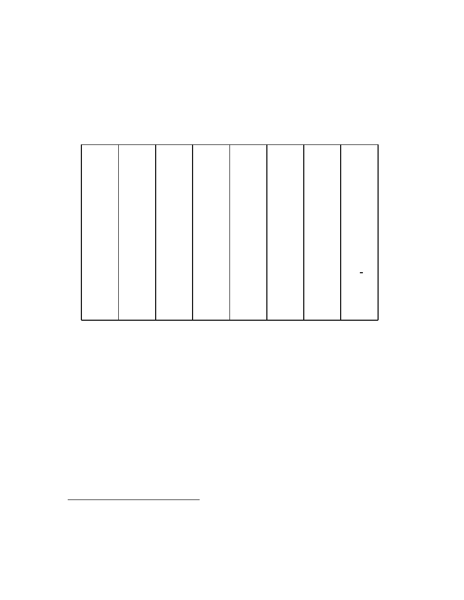
11
Figure 1.5: The ASCII Character Set
00 NUL
01 SOH
02 STX
03 ETX
04 EOT
05 ENQ
06 ACK
07 BEL
08 BS
09 HT
0A NL
0B VT
0C NP
0D CR
0E SO
0F SI
10 DLE
11 DC1
12 DC2
13 DC3
14 DC4
15 NAK
16 SYN
17 ETB
18 CAN
19 EM
1A SUB
1B ESC
1C FS
1D GS
1E RS
1F US
20 SP
21 !
22 "
23 #
24 $
25 %
26 &
27 ’
28 (
29 )
2A *
2B +
2C ,
2D -
2E .
2F /
30 0
31 1
32 2
33 3
34 4
35 5
36 6
37 7
38 8
39 9
3A :
3B ;
3C <
3D =
3E >
3F ?
40 @
41 A
42 B
43 C
44 D
45 E
46 F
47 G
48 H
49 I
4A J
4B K
4C L
4D M
4E N
4F O
50 P
51 Q
52 R
53 S
54 T
55 U
56 V
57 W
58 X
59 Y
5A Z
5B [
5C
5D ]
5E ^
5F
60 `
61 a
62 b
63 c
64 d
65 e
66 f
67 g
68 h
69 i
6A j
6B k
6C l
6D m
6E n
6F o
70 p
71 q
72 r
73 s
74 t
75 u
76 v
77 w
78 x
79 y
7A z
7B
{
7C |
7D
}
7E ~
7F DEL
or Japanese). Already new character sets which address these problems (and can be
used to represent characters of many languages side by side) are being proposed, and
eventually there will unquestionably be a shift away from ASCII to a new multilan-
guage standard
1
.
1.3
Representing Programs
Just as groups of bits can be used to represent numbers, they can also be used
to represent instructions for a computer to perform. Unlike the two’s complement
notation for integers, which is a standard representation used by nearly all computers,
the representation of instructions, and even the set of instructions, varies widely from
one type of computer to another.
The MIPS architecture, which is the focus of later chapters in this document, uses
1
This shift will break many, many existing programs. Converting all of these programs will keep
many, many programmers busy for some time.
12
CHAPTER 1.
DATA REPRESENTATION
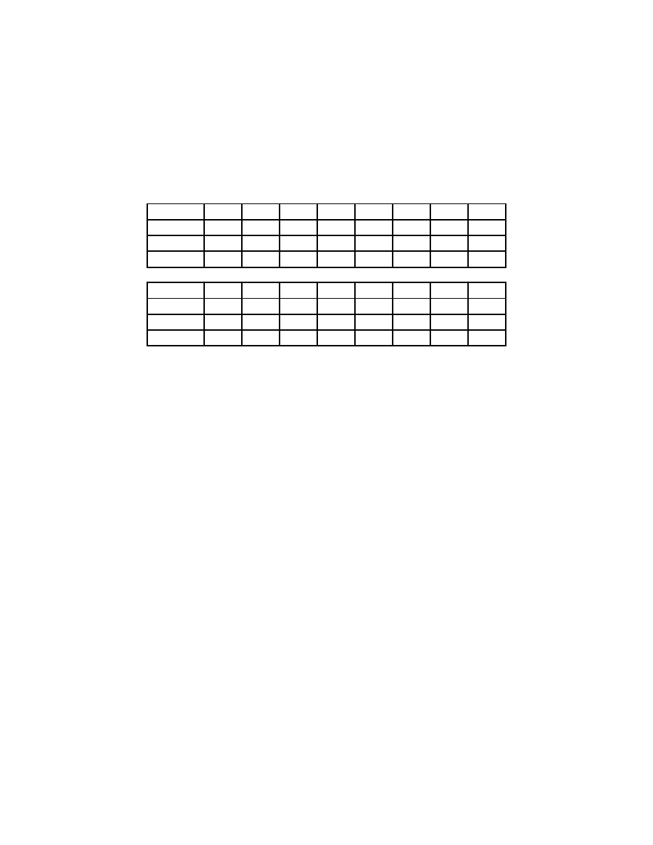
a relatively simple and straightforward representation. Each instruction is exactly 32
bits in length, and consists of several bit fields, as depicted in figure 1.6.
Figure 1.6: MIPS R2000 Instruction Formats
6 bits
5 bits
5 bits
5 bits
5 bits
6 bits
Register
op
reg1
reg2
des
shift
funct
Immediate
op
reg1
reg2
16-bit constant
Jump
op
26-bit constant
The first six bits (reading from the left, or high-order bits) of each instruction
are called the op field. The op field determines whether the instruction is a regis-
ter, immediate, or jump instruction, and how the rest of the instruction should be
interpreted. Depending on what the op is, parts of the rest of the instruction may
represent the names of registers, constant memory addresses, 16-bit integers, or other
additional qualifiers for the op.
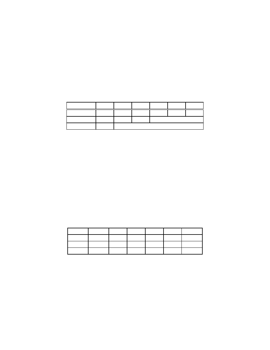
If the op field is 0, then the instruction is a register instruction, which generally
perform an arithmetic or logical operations. The funct field specifies the operation
to perform, while the reg1 and reg2 represent the registers to use as operands, and
the des field represents the register in which to store the result. For example, the
32-bit hexadecimal number 0x02918020 represents, in the MIPS instruction set, the
operation of adding the contents of registers 20 and 17 and placing the result in
register 16.
Field
op
reg1
reg2
des
shift
funct
Width
6 bits
5 bits
5 bits
5 bits
5 bits
6 bits
Values
0
20
17
16
0
add
Binary
000000 10100 10001 10000 00000 100000
If the op field is not 0, then the instruction may be either an immediate or jump
instruction, depending on the value of the op field.
1.4
Memory Organization
We’ve seen how sequences of binary digits can be used to represent numbers, char-
acters, and instructions. In a computer, these binary digits are organized and ma-

1.4.
MEMORY ORGANIZATION
13
nipulated in discrete groups, and these groups are said to be the memory of the
computer.
1.4.1
Units of Memory
The smallest of these groups, on most computers, is called a byte. On nearly all
currently popular computers a byte is composed of 8 bits.
The next largest unit of memory is usually composed of 16 bits. What this unit
is called varies from computer to computer– on smaller machines, this is often called
a word, while on newer architectures that can handle larger chunks of data, this is
called a halfword.
The next largest unit of memory is usually composed of 32 bits. Once again, the
name of this unit varies– on smaller machines, it is referred to as a long, while on
newer and larger machines it is called a word.
Finally, on the newest machines, the computer also can handle data in groups of
64 bits. On a smaller machine, this is known as a quadword, while on a larger machine
this is known as a long.
1.4.1.1
Historical Perspective
There have been architectures that have used nearly every imaginable word size– from
6-bit bytes to 9-bit bytes, and word sizes ranging from 12 bits to 48 bits. There are
even a few architectures that have no fixed word size at all (such as the CM-2) or
word sizes that can be specified by the operating system at runtime.
Over the years, however, most architectures have converged on 8-bit bytes and
32-bit longwords. An 8-bit byte is a good match for the ASCII character set (which
has some popular extensions that require 8 bits), and a 32-bit word has been, at least
until recently, large enough for most practical purposes.
1.4.2
Addresses and Pointers
Each unique byte
2
of the computer’s memory is given a unique identifier, known as
its address. The address of a piece of memory is often refered to as a pointer to that
2
In some computers, the smallest distinct unit of memory is not a byte. For the sake of simplicity,
however, this section assumes that the smallest distinct unit of memory on the computer in question
is a byte.

14
CHAPTER 1.
DATA REPRESENTATION
piece of memory– the two terms are synonymous, although there are many contexts
where one is commonly used and the other is not.
The memory of the computer itself can often be thought of as a large array (or
group of arrays) of bytes of memory. In this model, the address of each byte of
memory is simply the index of the memory array location where that byte is stored.
1.4.3
Summary
In this chapter, we’ve seen how computers represent integers using groups of bits, and
how basic arithmetic and other operations can be performed using this representation.
We’ve also seen how the integers or groups of bits can be used to represent sev-
eral different kinds of data, including written characters (using the ASCII character
codes), instructions for the computer to execute, and addresses or pointers, which
can be used to reference other data.
There are also many other ways that information can be represented using groups
of bits, including representations for rational numbers (usually by a representation
called floating point), irrational numbers, graphics, arbitrary character sets, and so
on. These topics, unfortunately, are beyond the scope of this book.
1.5.
EXERCISES
15
1.5
Exercises
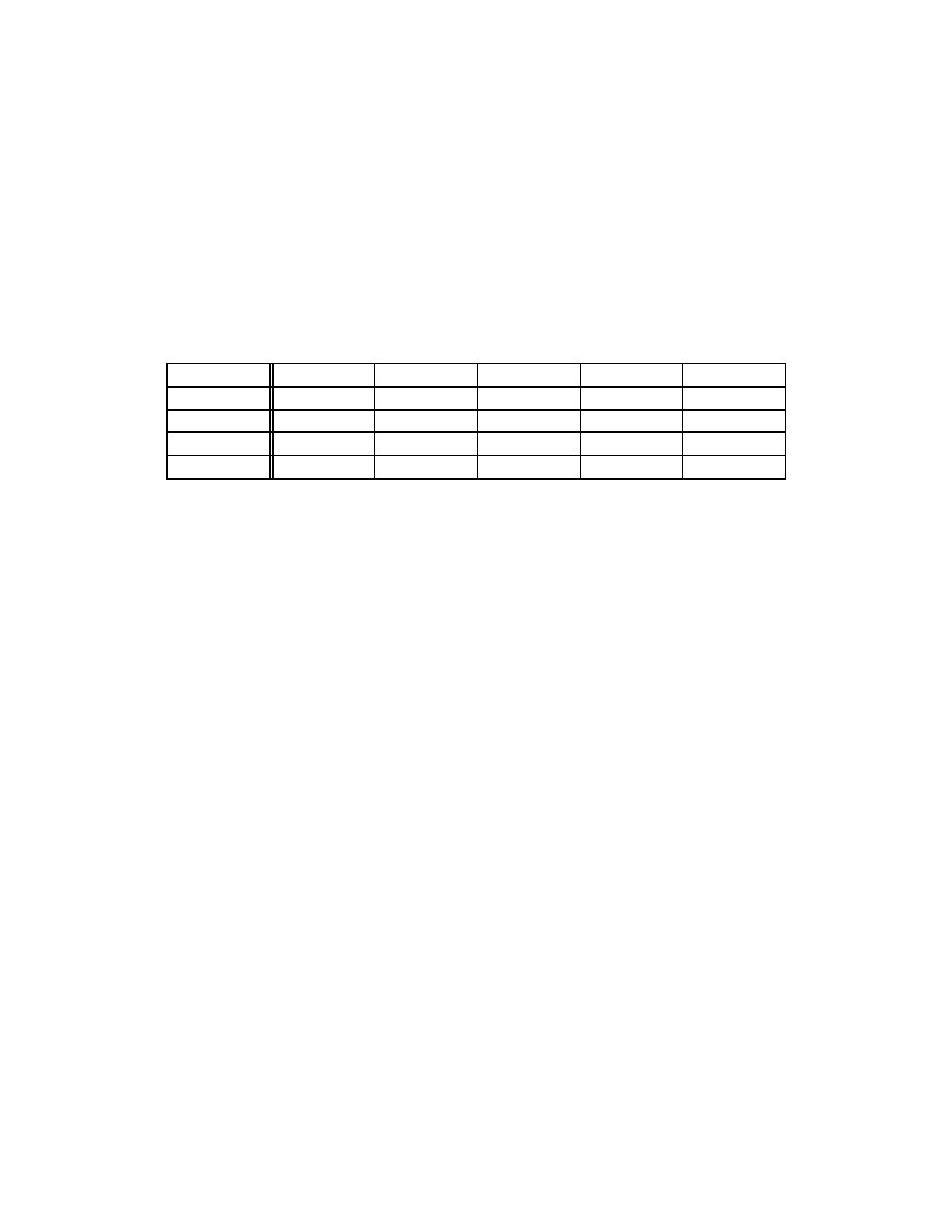
1.5.1
Complete the following table:
Decimal
123
Binary
01101100
Octal
143
Hex
3D
ASCII
Z
1.5.2
1. Invent an algorithm for multiplying two unsigned binary numbers. You may
find it easiest to start by thinking about multiplication of decimal numbers
(there are other ways as well, but you should start on familiar ground).
1.5.3
1. Invent an algorithm for dividing two unsigned binary numbers. You may find
it easiest to start by thinking about long division of decimal numbers.
2. Your TF complains that the division algorithm you invented to solve the pre-
vious part of this problem is too slow. She would prefer an algorithm that gets
an answer that is “reasonably close” to the right answer, but which may take
considerably less time to compute. Invent an algorithm that has this prop-
erty. Find the relationship between “reasonably close” and the speed of your
algorithm.

16
CHAPTER 1.
DATA REPRESENTATION

Chapter 2
MIPS Tutorial
by Daniel J. Ellard
This section is a quick tutorial for MIPS assembly language programming and the
SPIM environment
1
. This chapter covers the basics of MIPS assembly language, in-
cluding arithmetic operations, simple I/O, conditionals, loops, and accessing memory.
2.1
What is Assembly Language?
As we saw in the previous chapter, computer instructions can be represented as
sequences of bits. Generally, this is the lowest possible level of representation for a
program– each instruction is equivalent to a single, indivisible action of the CPU.
This representation is called machine language, since it is the only form that can be
“understood” directly by the machine.
A slightly higher-level representation (and one that is much easier for humans to
use) is called assembly language. Assembly language is very closely related to machine
language, and there is usually a straightforward way to translate programs written
in assembly language into machine language. (This algorithm is usually implemented
by a program called the assembler.) Because of the close relationship between ma-
1
For more detailed information about the MIPS instruction set and the SPIM environment, con-
sult chapter 4 of this book, and SPIM S20: A MIPS R2000 Simulator by James Larus. Other
references include Computer Organization and Design, by David Patterson and John Hennessy
(which includes an expanded version of James Larus’ SPIM documentation as appendix A), and
MIPS R2000 RISC Architecture
by Gerry Kane.
17

18
CHAPTER 2.
MIPS TUTORIAL
chine and assembly languages, each different machine architecture usually has its own
assembly language (in fact, each architecture may have several), and each is unique
2
.
The advantage of programming in assember (rather than machine language) is
that assembly language is much easier for a human to read and understand. For
example, the MIPS machine language instruction for adding the contents of registers
20 and 17 and placing the result in register 16 is the integer 0x02918020. This
representation is fairly impenetrable; given this instruction, it is not at all obvious
what it does– and even after you figure that out, it is not obvious, how to change the
result register to be register 12.
In the meanwhile, however, the MIPS assembly instruction for the same operation
is:
add
$16, $20, $17
This is much more readable– without knowing anything whatsoever about MIPS
assembly language, from the add it seems likely that addition is somehow involved,
and the operands of the addition are somehow related to the numbers 16, 20, and
17. A scan through the tables in the next chapter of this book confirms that add
performs addition, and that the first operand is the register in which to put the sum
of the registers indicated by the second and third operands. At this point, it is clear
how to change the result register to 12!
2.2
Getting Started: add.asm
To get our feet wet, we’ll write an assembly language program named add.asm that
computes the sum of 1 and 2, and stores the result in register $t0.
2.2.1
Commenting
Before we start to write the executable statements of program, however, we’ll need
to write a comment that describes what the program is supposed to do. In the MIPS
assembly language, any text between a pound sign (#) and the subsequent newline
2
For many years, considerable effort was spent trying to develop a portable assembly which
could generate machine language for a wide variety of architectures. Eventually, these efforts were
abandoned as hopeless.

2.2.
GETTING STARTED: ADD.ASM
19
is considered to be a comment. Comments are absolutely essential! Assembly lan-
guage programs are notoriously difficult to read unless they are properly documented.
Therefore, we start by writing the following:
# Daniel J. Ellard -- 02/21/94
# add.asm-- A program that computes the sum of 1 and 2,
#
leaving the result in register $t0.
# Registers used:
#
t0
- used to hold the result.
# end of add.asm
Even though this program doesn’t actually do anything yet, at least anyone read-
ing our program will know what this program is supposed to do, and who to blame
if it doesn’t work
3
. We are not finished commenting this program, but we’ve done
all that we can do until we know a little more about how the program will actually
work.
2.2.2
Finding the Right Instructions
Next, we need to figure out what instructions the computer will need to execute in
order to add two numbers. Since the MIPS architecture has relatively few instructions,
it won’t be long before you have memorized all of the instructions that you’ll need, but
as you are getting started you’ll need to spend some time browsing through the lists of
instructions, looking for ones that you can use to do what you want. Documentation
for the MIPS instruction set can be found in chapter 4 of this document.
Luckily, as we look through the list of arithmetic instructions, we notice the add
instruction, which adds two numbers together.
The add operation takes three operands:
1. A register that will be used to store the result of the addition. For our program,
this will be $t0.
2. A register which contains the first number to be added.
Therefore, we’re going to have to get 1 into a register before we can use it as
an operand of add. Checking the list of registers used by this program (which
3
You should put your own name on your own programs, of course; Dan Ellard shouldn’t take all
the blame.

20
CHAPTER 2.
MIPS TUTORIAL
is an essential part of the commenting) we select $t1, and make note of this in
the comments.
3. A register which holds the second number, or a 32-bit constant. In this case,
since 2 is a constant that fits in 32 bits, we can just use 2 as the third operand
of add.
We now know how we can add the numbers, but we have to figure out how to get
1 into register $t1. To do this, we can use the li (load immediate value) instruction,
which loads a 32-bit constant into a register. Therefore, we arrive at the following
sequence of instructions:
# Daniel J. Ellard -- 02/21/94
# add.asm-- A program that computes the sum of 1 and 2,
#
leaving the result in register $t0.
# Registers used:
#
t0
- used to hold the result.
#
t1
- used to hold the constant 1.
li
$t1, 1
# load 1 into $t1.
add
$t0, $t1, 2
# $t0 = $t1 + 2.
# end of add.asm
2.2.3
Completing the Program
These two instructions perform the calculation that we want, but they do not form
a complete program. Much like C, an assembly language program must contain some
additional information that tells the assembler where the program begins and ends.
The exact form of this information varies from assembler to assembler (note that
there may be more than one assembler for a given architecture, and there are several
for the MIPS architecture). This tutorial will assume that SPIM is being used as the
assembler and runtime environment.
2.2.3.1
Labels and main
To begin with, we need to tell the assembler where the program starts. In SPIM,
program execution begins at the location with the label main. A label is a symbolic
name for an address in memory. In MIPS assembly, a label is a symbol name (following
the same conventions as C symbol names), followed by a colon. Labels must be the

2.2.
GETTING STARTED: ADD.ASM
21
first item on a line. A location in memory may have more than one label. Therefore, to
tell SPIM that it should assign the label main to the first instruction of our program,
we could write the following:
# Daniel J. Ellard -- 02/21/94
# add.asm-- A program that computes the sum of 1 and 2,
#
leaving the result in register $t0.
# Registers used:
#
t0
- used to hold the result.
#
t1
- used to hold the constant 1.
main:
li
$t1, 1
# load 1 into $t1.
add
$t0, $t1, 2
# $t0 = $t1 + 2.
# end of add.asm
When a label appears alone on a line, it refers to the following memory location.
Therefore, we could also write this with the label main on its own line. This is
often much better style, since it allows the use of long, descriptive labels without
disrupting the indentation of the program. It also leaves plenty of space on the line
for the programmer to write a comment describing what the label is used for, which
is very important since even relatively short assembly language programs may have
a large number of labels.
Note that the SPIM assembler does not permit the names of instructions to be used
as labels. Therefore, a label named add is not allowed, since there is an instruction of
the same name. (Of course, since the instruction names are all very short and fairly
general, they don’t make very descriptive label names anyway.)
Giving the main label its own line (and its own comment) results in the following
program:
# Daniel J. Ellard -- 02/21/94
# add.asm-- A program that computes the sum of 1 and 2,
#
leaving the result in register $t0.
# Registers used:
#
t0
- used to hold the result.
#
t1
- used to hold the constant 1.
main:
# SPIM starts execution at main.
li
$t1, 1
# load 1 into $t1.
add
$t0, $t1, 2
# $t0 = $t1 + 2.
# end of add.asm

22
CHAPTER 2.
MIPS TUTORIAL
2.2.3.2
Syscalls
The end of a program is defined in a very different way. Similar to C, where the exit
function can be called in order to halt the execution of a program, one way to halt a
MIPS program is with something analogous to calling exit in C. Unlike C, however,
if you forget to “call exit” your program will not gracefully exit when it reaches the
end of the main function. Instead, it will blunder on through memory, interpreting
whatever it finds as instructions to execute
4
. Generally speaking, this means that
if you are lucky, your program will crash immediately; if you are unlucky, it will do
something random and then crash.
The way to tell SPIM that it should stop executing your program, and also to do
a number of other useful things, is with a special instruction called a syscall. The
syscall
instruction suspends the execution of your program and transfers control to
the operating system. The operating system then looks at the contents of register
$v0
to determine what it is that your program is asking it to do.
Note that SPIM syscalls are not real syscalls; they don’t actually transfer control to
the UNIX operating system. Instead, they transfer control to a very simple simulated
operating system that is part of the SPIM program.
In this case, what we want is for the operating system to do whatever is necessary
to exit our program. Looking in table 4.6.1, we see that this is done by placing a 10
(the number for the exit syscall) into $v0 before executing the syscall instruction.
We can use the li instruction again in order to do this:
# Daniel J. Ellard -- 02/21/94
# add.asm-- A program that computes the sum of 1 and 2,
#
leaving the result in register $t0.
# Registers used:
#
t0
- used to hold the result.
#
t1
- used to hold the constant 1.
#
v0
- syscall parameter.
main:
# SPIM starts execution at main.
li
$t1, 1
# load 1 into $t1.
add
$t0, $t1, 2
# compute the sum of $t1 and 2, and
# put it into $t0.
li
$v0, 10
# syscall code 10 is for exit.
syscall
# make the syscall.
4
You can “return” from main, just as you can in C, if you treat main as a function. See section 3.1
for more information.

2.3.
USING SPIM
23
# end of add.asm
2.3
Using SPIM
At this point, we should have a working program. Now, it’s time to try running it to
see what happens.
To run SPIM, simply enter the command spim at the commandline. SPIM will
print out a message similar to the following
5
:
% spim
SPIM Version 5.4 of Jan. 17, 1994
Copyright 1990-1994 by James R. Larus (larus@cs.wisc.edu).
All Rights Reserved.
See the file README a full copyright notice.
Loaded: /home/usr6/cs51/de51/SPIM/lib/trap.handler
(spim)
Whenever you see the (spim) prompt, you know that SPIM is ready to execute
a command. In this case, since we want to run the program that we just wrote, the
first thing we need to do is load the file containing the program. This is done with
the load command:
(spim) load "add.asm"
The load command reads and assembles a file containing MIPS assembly lan-
guage, and then loads it into the SPIM memory. If there are any errors during the
assembly, error messages with line number are displayed. You should not try to ex-
ecute a file that has not loaded successfully– SPIM will let you run the program, but
it is unlikely that it will actually work.
Once the program is loaded, you can use the run command to execute it:
(spim) run
The program runs, and then SPIM indicates that it is ready to execute another
command. Since our program is supposed to leave its result in register $t0, we can
verify that the program is working by asking SPIM to print out the contents of $t0,
using the print command, to see if it contains the result we expect:
5
The exact text will be different on different computers.

24
CHAPTER 2.
MIPS TUTORIAL
(spim) print $t0
Reg 8 = 0x00000003 (3)
The print command displays the register number followed by its contents in both
hexadecimal and decimal notation. Note that SPIM automatically translates from
the symbolic name for the register (in this case, $t0) to the actual register number
(in this case, $8).
2.4
Using syscall: add2.asm
Our program to compute 1+2 is not particularly useful, although it does demonstrate
a number of important details about programming in MIPS assembly language and
the SPIM environment. For our next example, we’ll write a program named add2.asm
that computes the sum of two numbers specified by the user at runtime, and displays
the result on the screen.
The algorithm this program will follow is:
1. Read the two numbers from the user.
We’ll need two registers to hold these two numbers. We can use $t0 and $t1
for this.
2. Compute their sum.
We’ll need a register to hold the result of this addition. We can use $t2 for this.
3. Print the sum.
4. Exit. We already know how to do this, using syscall.
Once again, we start by writing a comment. From what we’ve learned from
writing add.asm, we actually know a lot about what we need to do; the rest we’ll
only comment for now:
# Daniel J. Ellard -- 02/21/94
# add2.asm-- A program that computes and prints the sum
#
of two numbers specified at runtime by the user.
# Registers used:
#
$t0
- used to hold the first number.
#
$t1
- used to hold the second number.
#
$t2
- used to hold the sum of the $t1 and $t2.

2.4.
USING SYSCALL: ADD2.ASM
25
#
$v0
- syscall parameter.
main:
## Get first number from user, put into $t0.
## Get second number from user, put into $t1.
add
$t2, $t0, $t1
# compute the sum.
## Print out $t2.
li
$v0, 10
# syscall code 10 is for exit.
syscall
# make the syscall.
# end of add2.asm.
2.4.1
Reading and Printing Integers
The only parts of the algorithm that we don’t know how to do yet are to read the
numbers from the user, and print out the sum. Luckily, both of these operations can
be done with a syscall. Looking again in table 4.6.1, we see that syscall 5 can be
used to read an integer into register $v0, and and syscall 1 can be used to print
out the integer stored in $a0.
The syscall to read an integer leaves the result in register $v0, however, which
is a small problem, since we want to put the first number into $t0 and the second
into $t1. Luckily, in section 4.4.4.3 we find the move instruction, which copies the
contents of one register into another.
Note that there are good reasons why we need to get the numbers out of $v0
and move them into other registers: first, since we need to read in two integers, we’ll
need to make a copy of the first number so that when we read in the second number,
the first isn’t lost. In addition, when reading through the register use guidelines (in
section 4.3), we see that register $v0 is not a recommended place to keep anything,
so we know that we shouldn’t leave the second number in $v0 either.
This gives the following program:
# Daniel J. Ellard -- 02/21/94
# add2.asm-- A program that computes and prints the sum
#
of two numbers specified at runtime by the user.
# Registers used:
#
$t0
- used to hold the first number.
#
$t1
- used to hold the second number.

26
CHAPTER 2.
MIPS TUTORIAL
#
$t2
- used to hold the sum of the $t1 and $t2.
#
$v0
- syscall parameter and return value.
#
$a0
- syscall parameter.
main:
## Get first number from user, put into $t0.
li
$v0, 5
# load syscall read_int into $v0.
syscall
# make the syscall.
move
$t0, $v0
# move the number read into $t0.
## Get second number from user, put into $t1.
li
$v0, 5
# load syscall read_int into $v0.
syscall
# make the syscall.
move
$t1, $v0
# move the number read into $t1.
add
$t2, $t0, $t1
# compute the sum.
## Print out $t2.
move
$a0, $t2
# move the number to print into $a0.
li
$v0, 1
# load syscall print_int into $v0.
syscall
# make the syscall.
li
$v0, 10
# syscall code 10 is for exit.
syscall
# make the syscall.
# end of add2.asm.
2.5
Strings: the hello Program
The next program that we will write is the “Hello World” program. Looking in
table 4.6.1 once again, we note that there is a syscall to print out a string. All we
need to do is to put the address of the string we want to print into register $a0, the
constant 4 into $v0, and execute syscall. The only things that we don’t know how
to do are how to define a string, and then how to determine its address.
The string "Hello World" should not be part of the executable part of the pro-
gram (which contains all of the instructions to execute), which is called the text
segment of the program. Instead, the string should be part of the data used by the
program, which is, by convention, stored in the data segment. The MIPS assembler
allows the programmer to specify which segment to store each item in a program by
the use of several assembler directives. (see 4.5.1 for more information)

2.5.
STRINGS: THE HELLO PROGRAM
27
To put something in the data segment, all we need to do is to put a .data before
we define it. Everything between a .data directive and the next .text directive (or
the end of the file) is put into the data segment. Note that by default, the assembler
starts in the text segment, which is why our earlier programs worked properly even
though we didn’t explicitly mention which segment to use. In general, however, it is
a good idea to include segment directives in your code, and we will do so from this
point on.
We also need to know how to allocate space for and define a null-terminated string.
In the MIPS assembler, this can be done with the .asciiz (ASCII, zero terminated
string) directive. For a string that is not null-terminated, the .ascii directive can
be used (see 4.5.2 for more information).
Therefore, the following program will fulfill our requirements:
# Daniel J. Ellard -- 02/21/94
# hello.asm-- A "Hello World" program.
# Registers used:
#
$v0
- syscall parameter and return value.
#
$a0
- syscall parameter-- the string to print.
.text
main:
la
$a0, hello_msg
# load the addr of hello_msg into $a0.
li
$v0, 4
# 4 is the print_string syscall.
syscall
# do the syscall.
li
$v0, 10
# 10 is the exit syscall.
syscall
# do the syscall.
# Data for the program:
.data
hello_msg:
.asciiz "Hello World\n"
# end hello.asm
Note that data in the data segment is assembled into adjacent locations. There-
fore, there are many ways that we could have declared the string "Hello World\n"
and gotten the same exact output. For example we could have written our string as:
.data
hello_msg:
.ascii
"Hello" # The word "Hello"
.ascii
" "
# the space.

28
CHAPTER 2.
MIPS TUTORIAL
.ascii
"World" # The word "World"
.ascii
"\n"
# A newline.
.byte
0
# a 0 byte.
If we were in a particularly cryptic mood, we could have also written it as:
.data
hello_msg:
.byte 0x48
# hex for ASCII "H"
.byte 0x65
# hex for ASCII "e"
.byte 0x6C
# hex for ASCII "l"
.byte 0x6C
# hex for ASCII "l"
.byte 0x6F
# hex for ASCII "o"
...
# and so on...
.byte 0xA
# hex for ASCII newline
.byte 0x0
# hex for ASCII NUL
You can use the .data and .text directives to organize the code and data in
your programs in whatever is most stylistically appropriate. The example programs
generally have the all of the .data items defined at the end of the program, but this
is not necessary. For example, the following code will assemble to exactly the same
program as our original hello.asm:
.text
# put things into the text segment...
main:
.data
# put things into the data segment...
hello_msg:
.asciiz "Hello World\n"
.text
# put things into the text segment...
la
$a0, hello_msg
# load the addr of hello_msg into $a0.
li
$v0, 4
# 4 is the print_string syscall.
syscall
# do the syscall.
li
$v0, 10
# 10 is the exit syscall.
syscall
# do the syscall.
2.6
Conditional Execution: the larger Program
The next program that we will write will explore the problems of implementing condi-
tional execution in MIPS assembler language. The actual program that we will write
will read two numbers from the user, and print out the larger of the two.
One possible algorithm for this program is exactly the same as the one used
by add2.asm, except that we’re computing the maximum rather than the sum of

2.6.
CONDITIONAL EXECUTION: THE LARGER PROGRAM
29
two numbers. Therefore, we’ll start by copying add2.asm, but replacing the add
instruction with a placeholder comment:
# Daniel J. Ellard -- 02/21/94
# larger.asm-- prints the larger of two numbers specified
#
at runtime by the user.
# Registers used:
#
$t0
- used to hold the first number.
#
$t1
- used to hold the second number.
#
$t2
- used to store the larger of $t1 and $t2.
.text
main:
## Get first number from user, put into $t0.
li
$v0, 5
# load syscall read_int into $v0.
syscall
# make the syscall.
move
$t0, $v0
# move the number read into $t0.
## Get second number from user, put into $t1.
li
$v0, 5
# load syscall read_int into $v0.
syscall
# make the syscall.
move
$t1, $v0
# move the number read into $t1.
## put the larger of $t0 and $t1 into $t2.
## (placeholder comment)
## Print out $t2.
move
$a0, $t2
# move the number to print into $a0.
li
$v0, 1
# load syscall print_int into $v0.
syscall
# make the syscall.
## exit the program.
li
$v0, 10
# syscall code 10 is for exit.
syscall
# make the syscall.
# end of larger.asm.
Browsing through the instruction set again, we find in section 4.4.3.1 a description
of the MIPS branching instructions. These allow the programmer to specify that
execution should branch (or jump) to a location other than the next instruction. These
instructions allow conditional execution to be implemented in assembler language
(although in not nearly as clean a manner as higher-level languages provide).

30
CHAPTER 2.
MIPS TUTORIAL
One of the branching instructions is bgt. The bgt instruction takes three argu-
ments. The first two are numbers, and the last is a label. If the first number is larger
than the second, then execution should continue at the label, otherwise it continues
at the next instruction. The b instruction, on the other hand, simply branches to the
given label.
These two instructions will allow us to do what we want. For example, we could
replace the placeholder comment with the following:
# If $t0 > $t1, branch to t0_bigger,
bgt
$t0, $t1, t0_bigger
move
$t2, $t1
# otherwise, copy $t1 into $t2.
b
endif
# and then branch to endif
t0_bigger:
move
$t2, $t0
# copy $t0 into $t2
endif:
If $t0 is larger, then execution will branch to the t0_bigger label, where $t0 will
be copied to $t2. If it is not, then the next instructions, which copy $t1 into $t2
and then branch to the endif label, will be executed.
This gives us the following program:
# Daniel J. Ellard -- 02/21/94
# larger.asm-- prints the larger of two numbers specified
#
at runtime by the user.
# Registers used:
#
$t0
- used to hold the first number.
#
$t1
- used to hold the second number.
#
$t2
- used to store the larger of $t1 and $t2.
#
$v0
- syscall parameter and return value.
#
$a0
- syscall parameter.
.text
main:
## Get first number from user, put into $t0.
li
$v0, 5
# load syscall read_int into $v0.
syscall
# make the syscall.
move
$t0, $v0
# move the number read into $t0.
## Get second number from user, put into $t1.
li
$v0, 5
# load syscall read_int into $v0.
syscall
# make the syscall.
move
$t1, $v0
# move the number read into $t1.

2.7.
LOOPING: THE MULTIPLES PROGRAM
31
## put the larger of $t0 and $t1 into $t2.
bgt
$t0, $t1, t0_bigger
# If $t0 > $t1, branch to t0_bigger,
move
$t2, $t1
# otherwise, copy $t1 into $t2.
b
endif
# and then branch to endif
t0_bigger:
move
$t2, $t0
# copy $t0 into $t2
endif:
## Print out $t2.
move
$a0, $t2
# move the number to print into $a0.
li
$v0, 1
# load syscall print_int into $v0.
syscall
# make the syscall.
## exit the program.
li
$v0, 10
# syscall code 10 is for exit.
syscall
# make the syscall.
# end of larger.asm.
2.7
Looping: the multiples Program
The next program that we will write will read two numbers A and B, and print out
multiples of A from A to A × B. The algorithm that our program will use is given in
algorithm 2.1. This algorithm translates easily into MIPS assembly. Since we already
know how to read in numbers and print them out, we won’t bother to implement
these steps here– we’ll just leave these as comments for now.
# Daniel J. Ellard -- 02/21/94
# multiples.asm-- takes two numbers A and B, and prints out
#
all the multiples of A from A to A * B.
#
If B <= 0, then no multiples are printed.
# Registers used:
#
$t0
- used to hold A.
#
$t1
- used to hold B.
#
$t2
- used to store S, the sentinel value A * B.
#
$t3
- used to store m, the current multiple of A.
.text
main:
## read A into $t0, B into $t1 (omitted).

32
CHAPTER 2.
MIPS TUTORIAL
Algorithm 2.1
The multiples program.
1. Get A from the user.
2. Get B from the user. If B ≤ 0, terminate.
3. Set sentinel value S = A × B.
4. Set multiple m = A.
5. Loop:
(a) Print m.
(b) If m == S, then go to the next step.
(c) Otherwise, set m = m + A, and then repeat the loop.
6. Terminate.

2.8.
LOADS: THE PALINDROME.ASM PROGRAM
33
blez
$t1, exit
# if B <= 0, exit.
mul
$t2, $t0, $t1
# S = A * B.
move
$t3, $t0
# m = A
loop:
## print out $t3 (omitted)
beq
$t2, $t3, endloop
# if m == S, we’re done.
add
$t3, $t3, $t0
# otherwise, m = m + A.
## print a space (omitted)
b
loop
endloop:
## exit (omitted)
# end of multiples.asm
The complete code for this program is listed in section 5.3.
2.8
Loads: the palindrome.asm Program
The next program that we write will read a line of text and determine whether or
not the text is a palindrome. A palindrome is a word or sentence that spells exactly
the same thing both forward and backward. For example, the string “anna” is a
palindrome, while “ann” is not. The algorithm that we’ll be using to determine
whether or not a string is a palindrome is given in algorithm 2.2.
Note that in the more common definition of a palindrome, whitespace, capitaliza-
tion, and punctuation are ignored, so the string “Able was I ere I saw Elba.” would
be considered a palindrome, but by our definition it is not. (In exercise 2.10.2, you
get to fix this oversight.)
Once again, we start with a comment:
## Daniel J. Ellard -- 02/21/94
## palindrome.asm -- reads a line of text and tests if it is a palindrome.
## Register usage:
##
$t1
- A.
##
$t2
- B.
##
$t3
- the character at address A.
##
$t4
- the character at address B.
##
$v0
- syscall parameter / return values.

34
CHAPTER 2.
MIPS TUTORIAL
Algorithm 2.2
To determine if the string that starts at address S is a palindrome.
This algorithm is appropriate for the strings that end with a newline followed by a
0 character, as strings read in by the read string syscall do. (See exercise 2.10.1 to
generalize this algorithm.)
Note that in this algorithm, the operation of getting the character located at address
X
is written as ∗X.
1. Let A = S.
2. Let B = a pointer to the last character of S. To find the last character in S,
use the following algorithm:
(a) Let B = S.
(b) Loop:
• If ∗B == 0 (i.e. the character at address B is 0), then B has gone
past the end of the string. Set B = B − 2 (to move B back past the
0 and the newline), and continue with the next step.
• Otherwise, set B = (B + 1).
3. Loop:
(a) If A ≥ B, then the string is a palindrome. Halt.
(b) If ∗A 6= ∗B, then the string is not a palindrome. Halt.
(c) Set A = (A + 1).
(d) Set B = (B − 1).

2.8.
LOADS: THE PALINDROME.ASM PROGRAM
35
##
$a0
- syscall parameters.
##
$a1
- syscall parameters.
The first step of the algorithm is to read in the string from the user. This can be
done with the read_string syscall (syscall number 8), which is similar in function
to the fgets function in the C standard I/O library. To use this syscall, we need to
load into register $a0 the pointer to the start of the memory that we have set aside
to hold the string. We also need to load into register $a1 the maximum number of
bytes to read.
To set aside the space that we’ll need to need to store the string, the .space
directive can be used. This gives the following code:
.text
main:
# SPIM starts by jumping to main.
## read the string S:
la
$a0, string_space
li
$a1, 1024
li
$v0, 8
# load "read_string" code into $v0.
syscall
.data
string_space:
.space
1024
# set aside 1024 bytes for the string.
Once we’ve got the string, then we can use algorithm 2.2 (on page 34). The first
step is simple enough; all we need to do is load the address of string_space into
register $t1, the register that we’ve set aside to represent A:
la
$t1, string_space
# A = S.
The second step is more complicated. In order to compare the character pointed
to by B with 0, we need to load this character into a register. This can be done with
the lb (load byte) instruction:
la
$t2, string_space
## we need to move B to the end
length_loop:
#
of the string:
lb
$t3, ($t2)
# load the byte at B into $t3.
beqz
$t3, end_length_loop
# if $t3 == 0, branch out of loop.
addu
$t2, $t2, 1
# otherwise, increment B,
b
length_loop
#
and repeat
end_length_loop:
subu
$t2, $t2, 2
## subtract 2 to move B back past
#
the ’\0’ and ’\n’.

36
CHAPTER 2.
MIPS TUTORIAL
Note that the arithmetic done on the pointer B is done using unsigned arithmetic
(using addu and subu). Since there is no way to know where in memory a pointer
will point, the numerical value of the pointer may well be a “negative” number if it
is treated as a signed binary number .
When this step is finished, A points to the first character of the string and B points
to the last. The next step determines whether or not the string is a palindrome:
test_loop:
bge
$t1, $t2, is_palin
# if A >= B, it’s a palindrome.
lb
$t3, ($t1)
# load the byte at address A into $t3,
lb
$t4, ($t2)
# load the byte at address B into $t4.
bne
$t3, $t4, not_palin
# if $t3 != $t4, not a palindrome.
# Otherwise,
addu
$t1, $t1, 1
#
increment A,
subu
$t2, $t2, 1
#
decrement B,
b
test_loop
#
and repeat the loop.
The complete code for this program is listed in section 5.4 (on page 74).
2.9
The atoi Program
The next program that we’ll write will read a line of text from the terminal, interpret
it as an integer, and then print it out. In effect, we’ll be reimplementing the read_int
system call (which is similar to the GetInteger function in the Roberts libraries).
2.9.1
atoi-1
We already know how to read a string, and how to print out a number, so all we need
is an algorithm to convert a string into a number. We’ll start with the algorithm
given in 2.3 (on page 37).
Let’s assume that we can use register $t0 as S, register $t2 as D, and register
$t1
is available as scratch space. The code for this algorithm then is simply:
li
$t2, 0
# Initialize sum = 0.
sum_loop:
lb
$t1, ($t0)
# load the byte *S into $t1,
addu
$t0, $t0, 1
# and increment S.

2.9.
THE ATOI PROGRAM
37
Algorithm 2.3
To convert an ASCII string representation of a integer into the cor-
responding integer.
Note that in this algorithm, the operation of getting the character at address X is
written as ∗X.
• Let S be a pointer to start of the string.
• Let D be the number.
1. Set D = 0.
2. Loop:
(a) If ∗S == ’\n’, then continue with the next step.
(b) Otherwise,
i. S = (S + 1)
ii. D = (D × 10)
iii. D = (D + (∗S − ’0’))
In this step, we can take advantage of the fact that ASCII puts the
numbers with represent the digits 0 through 9 are arranged consecu-
tively, starting at 0. Therefore, for any ASCII character x, the number
represented by x is simply x − ’0’.

38
CHAPTER 2.
MIPS TUTORIAL
## use 10 instead of ’\n’ due to SPIM bug!
beq
$t1, 10, end_sum_loop
# if $t1 == \n, branch out of loop.
mul
$t2, $t2, 10
# t2 *= 10.
sub
$t1, $t1, ’0’
# t1 -= ’0’.
add
$t2, $t2, $t1
# t2 += t1.
b
sum_loop
#
and repeat the loop.
end_sum_loop:
Note that due to a bug in the SPIM assembler, the beq must be given the con-
stant 10 (which is the ASCII code for a newline) rather than the symbolic character
code ’\n’, as you would use in C. The symbol ’\n’ does work properly in strings
declarations (as we saw in the hello.asm program).
A complete program that uses this code is in atoi-1.asm.
2.9.2
atoi-2
Although the algorithm used by atoi-1 seems reasonable, it actually has several
problems. The first problem is that this routine cannot handle negative numbers.
We can fix this easily enough by looking at the very first character in the string, and
doing something special if it is a ’-’. The easiest thing to do is to introduce a new
variable, which we’ll store in register $t3, which represents the sign of the number. If
the number is positive, then $t3 will be 1, and if negative then $t3 will be -1. This
makes it possible to leave the rest of the algorithm intact, and then simply multiply
the result by $t3 in order to get the correct sign on the result at the end:
li
$t2, 0
# Initialize sum = 0.
get_sign:
li
$t3, 1
lb
$t1, ($t0)
# grab the "sign"
bne
$t1, ’-’, positive
# if not "-", do nothing.
li
$t3, -1
# otherwise, set t3 = -1, and
addu
$t0, $t0, 1
#
skip over the sign.
positive:
sum_loop:
## sum_loop is the same as before.

2.9.
THE ATOI PROGRAM
39
end_sum_loop:
mul
$t2, $t2, $t3
# set the sign properly.
A complete program that incorporates these changes is in atoi-2.asm.
2.9.3
atoi-3
While the algorithm in atoi-2.asm is better than the one used by atoi-1.asm, it is
by no means free of bugs. The next problem that we must consider is what happens
when S does not point to a proper string of digits, but instead points to a string that
contains erroneous characters.
If we want to mimic the behavior of the UNIX atoi library function, then as
soon as we encounter any character that isn’t a digit (after an optional ’-’) then we
should stop the conversion immediately and return whatever is in D as the result. In
order to implement this, all we need to do is add some extra conditions to test on
every character that gets read in inside sum_loop:
sum_loop:
lb
$t1, ($t0)
# load the byte *S into $t1,
addu
$t0, $t0, 1
# and increment S,
## use 10 instead of ’\n’ due to SPIM bug!
beq
$t1, 10, end_sum_loop
# if $t1 == \n, branch out of loop.
blt
$t1, ’0’, end_sum_loop
# make sure 0 <= t1
bgt
$t1, ’9’, end_sum_loop
# make sure 9 >= t1
mul
$t2, $t2, 10
# t2 *= 10.
sub
$t1, $t1, ’0’
# t1 -= ’0’.
add
$t2, $t2, $t1
# t2 += t1.
b
sum_loop
# and repeat the loop.
end_sum_loop:
A complete program that incorporates these changes is in atoi-3.asm.
2.9.4
atoi-4
While the algorithm in atoi-3.asm is nearly correct (and is at least as correct as the
one used by the standard atoi function), it still has an important bug. The problem

40
CHAPTER 2.
MIPS TUTORIAL
is that algorithm 2.3 (and the modifications we’ve made to it in atoi-2.asm and
atoi-3.asm
) is generalized to work with any number. Unfortunately, register $t2,
which we use to represent D, can only represent 32-bit binary number. Although
there’s not much that we can do to prevent this problem, we definitely want to detect
this problem and indicate that an error has occurred.
There are two spots in our routine where an overflow might occur: when we
multiply the contents of register $t2 by 10, and when we add in the value represented
by the current character.
Detecting overflow during multiplication is not hard. Luckily, in the MIPS archi-
tecture, when multiplication and division are performed, the result is actually stored
in two 32-bit registers, named lo and hi. For division, the quotient is stored in lo
and the remainder in hi. For multiplication, lo contains the low-order 32 bits and
hi
contains the high-order 32 bits of the result. Therefore, if hi is non-zero after we
do the multiplication, then the result of the multiplication is too large to fit into a
single 32-bit word, and we can detect the error.
We’ll use the mult instruction to do the multiplication, and then the mfhi (move
from hi) and mflo (move from lo) instructions to get the results.
To implement this we need to replace the single line that we used to use to do the
multiplication with the following:
# Note-- $t4 contains the constant 10.
mult
$t2, $t4
# multiply $t2 by 10.
mfhi
$t5
# check for overflow;
bnez
$t5, overflow
#
if so, then report an overflow.
mflo
$t2
# get the result of the multiply
There’s another error that can occur here, however: if the multiplication makes
the number too large to be represented as a positive two’s complement number, but
not quite large enough to require more than 32 bits. (For example, the number
3000000000 will be converted to -1294967296 by our current routine.) To detect
whether or not this has happened, we need to check whether or not the number in
register $t2 appears to be negative, and if so, indicate an error. This can be done by
adding the following instruction immediately after the mflo:
blt
$t2, $0, overflow
# make sure that it isn’t negative.
This takes care of checking that the multiplication didn’t overflow. We can detect
whether an addition overflowed in much the same manner, by adding the same test
immediately after the addition.

2.9.
THE ATOI PROGRAM
41
The resulting code, along with the rest of the program, can be found in section 5.6
(on page 78).

42
CHAPTER 2.
MIPS TUTORIAL
2.10
Exercises
2.10.1
In the palindrome algorithm 2.2, the algorithm for moving B to the end of the string
is incorrect if the string does not end with a newline.
Fix algorithm 2.2 so that it behaves properly whether or not there is a newline on
the end of the string. Once you have fixed the algorithm, fix the code as well.
2.10.2
Modify the palindrome.asm program so that it ignores whitespace, capitalization,
and punctuation.
Your program must be able to recognize the following strings as palindromes:
1. ”1 2 321”
2. ”Madam, I’m Adam.”
3. ”Able was I, ere I saw Elba.”
4. ”A man, a plan, a canal– Panama!”
5. ”Go hang a salami; I’m a lasagna hog.”
2.10.3
Write a MIPS assembly language program that asks the user for 20 numbers, bub-
blesorts them, and then prints them out in ascending order.

Chapter 3
Advanced MIPS Tutorial
by Daniel J. Ellard
This chapter continues the tutorial for MIPS assembly language programming and
the SPIM environment
1
. This chapter introduces more advanced topics, such as
how functions and advanced data structures can be implemented in MIPS assembly
language.
3.1
Function Environments and Linkage
One of the most important benefits of a high-level language such as C is the notion
of a function. In C, a function provides several useful abstractions:
• The mapping of actual parameters to formal parameters.
• Allocation and initialization of temporary local storage. This is particularly
important in languages which allow recursion: each call to the function must
get its own copy of any local variables, to prevent one call to a recursive function
from clobbering the values of a surrounding call to the same function.
1
For more detailed information about the MIPS instruction set and the SPIM environment, con-
sult chapter 4 of this book, and SPIM S20: A MIPS R2000 Simulator by James Larus. Other
references include Computer Organization and Design, by David Patterson and John Hennessy
(which includes an expanded version of James Larus’ SPIM documentation as appendix A), and
MIPS R2000 RISC Architecture
by Gerry Kane.
43

44
CHAPTER 3.
ADVANCED MIPS TUTORIAL
The information that describes the state of a function during execution (i.e. the
actual parameters, the value of all of the local variables, and which statement is
being executed) is called the environment of the function. (Note that the values of
any global variables referenced by the function are not part of the environment.) For
a MIPS assembly program, the environment of a function consists of the values of all
of the registers that are referenced in the function (see exercise 3.3.1).
In order to implement the ability to save and restore a function’s environment,
most architectures, including the MIPS, use the stack to store each of the environ-
ments.
In general, before a function A calls function B, it pushes its environment onto
the stack, and then jumps to function B. When the function B returns, function
A
restores its environment by popping it from the stack. In the MIPS software
architecture, this is accomplished with the following procedure:
1. The caller must:
(a) Put the parameters into $a0-$a3. If there are more than four parameters,
the additional parameters are pushed onto the stack.
(b) Save any of the caller-saved registers ($t0 - $t9) which are used by the
caller.
(c) Execute a jal (or jalr) to jump to the function.
2. The callee must, as part of the function preamble:
(a) Create a stack frame, by subtracting the frame size from the stack pointer
($sp).
Note that the minimum stack frame size in the MIPS software architecture
is 32 bytes, so even if you don’t need all of this space, you should still make
your stack frames this large.
(b) Save any callee-saved registers ($s0 - $s7, $fp, $ra) which are used by the
callee. Note that the frame pointer ($fp) must always be saved. The return
address ($ra) needs to be saved only by functions which make function calls
themselves.
(c) Set the frame pointer to the stack pointer, plus the frame size.
3. The callee then executes the body of the function.
4. To return from a function, the callee must:

3.1.
FUNCTION ENVIRONMENTS AND LINKAGE
45
(a) Put the return value, if any, into register $v0.
(b) Restore callee-saved registers.
(c) Jump back to $ra, using the jr instruction.
5. To clean up after a function call, the caller must:
(a) Restore the caller-saved registers.
(b) If any arguments were passed on the stack (instead of in $a0-$a3), pop
them off of the stack.
(c) Extract the return value, if any, from register $v0.
The convention used by the programs in this document is that a function stores
$fp
at the top of its stack frame, followed by $ra, then any of the callee-saved registers
($s0 - $s7), and finally any of the caller-saved registers ($t0 - $t9) that need to be
preserved.
3.1.1
Computing Fibonacci Numbers
The Fibonacci sequence has the following recursive definition: let F (n) be the nth
element (where n ≥ 0) in the sequence:
• If n < 2, then F (n) ≡ 1. (the base case)
• Otherwise, F (n) = F (n − 1) + F (n − 2). (the recursive case)
This definition leads directly to a recursive algorithm for computing the nth Fi-
bonacci number. As you may have realized, particularly if you’ve seen this sequence
before, there are much more efficient ways to compute the nth Fibonacci number.
Nevertheless, this algorithm is often used to demonstrate recursion– so here we go
again.
In order to demonstrate a few different aspects of the MIPS function calling con-
ventions, however, we’ll implement the fib function in a few different ways.
3.1.1.1
Using Saved Registers: fib-s.asm
The first way that we’ll code this will use callee-saved registers to hold all of the local
variables.

46
CHAPTER 3.
ADVANCED MIPS TUTORIAL
# fib-- (callee-save method)
# Registers used:
#
$a0
- initially n.
#
$s0
- parameter n.
#
$s1
- fib (n - 1).
#
$s2
- fib (n - 2).
.text
fib:
subu
$sp, $sp, 32
# frame size = 32, just because...
sw
$ra, 28($sp)
# preserve the Return Address.
sw
$fp, 24($sp)
# preserve the Frame Pointer.
sw
$s0, 20($sp)
# preserve $s0.
sw
$s1, 16($sp)
# preserve $s1.
sw
$s2, 12($sp)
# preserve $s2.
addu
$fp, $sp, 32
# move Frame Pointer to base of frame.
move
$s0, $a0
# get n from caller.
blt
$s0, 2, fib_base_case
# if n < 2, then do base case.
sub
$a0, $s0, 1
# compute fib (n - 1)
jal
fib
#
move
$s1, $v0
# s1 = fib (n - 1).
sub
$a0, $s0, 2
# compute fib (n - 2)
jal
fib
move
$s2, $v0
# $s2 = fib (n - 2).
add
$v0, $s1, $s2
# $v0 = fib (n - 1) + fib (n - 2).
b
fib_return
fib_base_case:
# in the base case, return 1.
li
$v0, 1
fib_return:
lw
$ra, 28($sp)
# restore the Return Address.
lw
$fp, 24($sp)
# restore the Frame Pointer.
lw
$s0, 20($sp)
# restore $s0.
lw
$s1, 16($sp)
# restore $s1.
lw
$s2, 12($sp)
# restore $s2.
addu
$sp, $sp, 32
# restore the Stack Pointer.
jr
$ra
# return.
As a baseline test, let’s time the execution of this program computing the F (20):

3.1.
FUNCTION ENVIRONMENTS AND LINKAGE
47
% echo 20 | /bin/time spim -file fib-s.asm
SPIM Version 5.4 of Jan. 17, 1994
Copyright 1990-1994 by James R. Larus (larus@cs.wisc.edu).
All Rights Reserved.
See the file README a full copyright notice.
Loaded: /home/usr6/cs51/de51/SPIM/lib/trap.handler
10946
5.1 real
4.8 user
0.2 sys
3.1.1.2
Using Temporary Registers: fib-t.asm
If you trace through the execution of the fib function in fib-s.asm, you’ll see that
roughly half of the function calls are leaf calls. Therefore, it is often unnecessary to
go to all of the work of saving all of the registers in each call to fib, since half the
time fib doesn’t call itself again. We can take advantage of this fact by using caller
saved registers (in this case $t0-$t2) instead of callee saved registers. Since it is the
responsibility of the caller to save these registers, the code gets somewhat rearranged:
# fib-- (caller-save method)
# Registers used:
#
$a0
- initially n.
#
$t0
- parameter n.
#
$t1
- fib (n - 1).
#
$t2
- fib (n - 2).
.text
fib:
subu
$sp, $sp, 32
# frame size = 32, just because...
sw
$ra, 28($sp)
# preserve the Return Address.
sw
$fp, 24($sp)
# preserve the Frame Pointer.
addu
$fp, $sp, 32
# move Frame Pointer to base of frame.
move
$t0, $a0
# get n from caller.
blt
$t0, 2, fib_base_case
# if n < 2, then do base case.
# call function fib (n - 1):
sw
$t0, 20($sp)
# save n.
sub
$a0, $t0, 1
# compute fib (n - 1)
jal
fib
move
$t1, $v0
# $t1 = fib (n - 1)
lw
$t0, 20($sp)
# restore n.
# call function fib (n - 2);
sw
$t0, 20($sp)
# save n.

48
CHAPTER 3.
ADVANCED MIPS TUTORIAL
sw
$t1, 16($sp)
# save $t1.
sub
$a0, $t0, 2
# compute fib (n - 2)
jal
fib
move
$t2, $v0
# $t2 = fib (n - 2)
lw
$t0, 20($sp)
# restore n.
lw
$t1, 16($sp)
# restore $t1.
add
$v0, $t1, $t2
# $v0 = fib (n - 1) + fib (n - 2).
b
fib_return
fib_base_case:
# in the base case, return 1.
li
$v0, 1
fib_return:
lw
$ra, 28($sp)
# Restore the Return Address.
lw
$fp, 24($sp)
# restore the Frame Pointer.
addu
$sp, $sp, 32
# restore the Stack Pointer.
jr
$ra
# return.
Once again, we can time the execution of this program in order to see if this
change has made any improvement:
% echo 20 | /bin/time spim -file fib-t.asm
SPIM Version 5.4 of Jan. 17, 1994
Copyright 1990-1994 by James R. Larus (larus@cs.wisc.edu).
All Rights Reserved.
See the file README a full copyright notice.
Loaded: /home/usr6/cs51/de51/SPIM/lib/trap.handler
10946
4.5 real
4.1 user
0.1 sys
In these tests, the user time is what we want to measure, and as we can see,
fib-s.asm
is approximately 17% slower than fib-t.asm.
3.1.1.3
Optimization: fib-o.asm
Warning! Hacks ahead! There are still more tricks we can try in order to increase the
performance of this program. Of course, the best way to increase the performance of
this program would be to use a better algorithm, but for now we’ll concentrate on
optimizing our assembly implementation of the algorithm we’ve been using.
Starting with the observation that about half the calls to fib have an argument n
of 1 or 0, and therefore do not need to do anything except return a 1, we can simplify
the program considerably: this base case doesn’t require building a stack frame, or

3.1.
FUNCTION ENVIRONMENTS AND LINKAGE
49
using any registers except $a0 and $v0. Therefore, we can postpone the work of
building a stack frame until after we’ve tested to see if we’re going to do the base
case.
In addition, we can further trim down the number of instructions that are executed
by saving fewer registers. For example, in the second recursive call to fib it is not
necessary to preserve n– we don’t care if it gets clobbered, since it isn’t used anywhere
after this call.
## fib-- (hacked-up caller-save method)
## Registers used:
##
$a0
- initially n.
##
$t0
- parameter n.
##
$t1
- fib (n - 1).
##
$t2
- fib (n - 2).
.text
fib:
bgt
$a0, 1, fib_recurse
# if n < 2, then just return a 1,
li
$v0, 1
# don’t bother to build a stack frame.
jr
$ra
# otherwise, set things up to handle
fib_recurse:
# the recursive case:
subu
$sp, $sp, 32
# frame size = 32, just because...
sw
$ra, 28($sp)
# preserve the Return Address.
sw
$fp, 24($sp)
# preserve the Frame Pointer.
addu
$fp, $sp, 32
# move Frame Pointer to base of frame.
move
$t0, $a0
# get n from caller.
# compute fib (n - 1):
sw
$t0, 20($sp)
# preserve n.
sub
$a0, $t0, 1
# compute fib (n - 1)
jal
fib
move
$t1, $v0
# t1 = fib (n - 1)
lw
$t0, 20($sp)
# restore n.
# compute fib (n - 2):
sw
$t1, 16($sp)
# preserve $t1.
sub
$a0, $t0, 2
# compute fib (n - 2)
jal
fib
move
$t2, $v0
# t2 = fib (n - 2)
lw
$t1, 16($sp)
# restore $t1.
add
$v0, $t1, $t2
# $v0 = fib (n - 1) + fib (n - 2)

50
CHAPTER 3.
ADVANCED MIPS TUTORIAL
lw
$ra, 28($sp)
# restore Return Address.
lw
$fp, 24($sp)
# restore Frame Pointer.
addu
$sp, $sp, 32
# restore Stack Pointer.
jr
$ra
# return.
Let’s time this and see how it compares:
% echo 20 | /bin/time spim -file fib-o.asm
SPIM Version 5.4 of Jan. 17, 1994
Copyright 1990-1994 by James R. Larus (larus@cs.wisc.edu).
All Rights Reserved.
See the file README a full copyright notice.
Loaded: /home/usr6/cs51/de51/SPIM/lib/trap.handler
10946
3.1 real
2.8 user
0.2 sys
This is clearly much faster. In fact, it’s nearly twice as fast as the original
fib-s.asm
. This makes sense, since we have eliminated building and destroying
about half of the stack frames, and a large percentage of the fib function does noth-
ing but set up and dismantle the stack frame.
Note that the reason that optimizing the base case of the recursion helps so much
with this algorithm is because it occurs about half of the time– but this is not charac-
teristic of all recursive algorithms. For example, in a recursive algorithm to compute
the factorial of n, the recursive case will occur about n − 1 times, while the base case
will only occur once. Therefore, it makes more sense to optimize the recursive case
in that situation.
There’s still more that can be done, however; see exercise 3.3.3 to pursue this
farther. A complete listing of a program that uses this implementation of the fib
function can be found in section 5.8 (on page 84).
3.2
Structures and sbrk: the treesort Program
Included in section 5.9 of this document is the source code for a SPIM program that
reads a list of numbers from the user and prints out the list in ascending order. The
input is read one number per line, using the read_int syscall, until the user types in
the sentinel value. The sentinel value is currently 0, but can be changed in the code
to any 32-bit integer.
The treesort algorithm should be familiar to anyone who has used ordered binary
trees. The general algorithm is shown in 3.1.

3.2.
STRUCTURES AND SBRK: THE TREESORT PROGRAM
51
Algorithm 3.1
The treesort algorithm.
1. Build an ordered binary tree T containing all the values to be sorted.
2. Do an inorder traversal of T , printing out the values of each node.
Since we already have seen how to write functions (including recursive functions),
doing the inorder traversal won’t be much of a problem. Building the tree, however,
will require several new techniques: we need to learn how to represent structures
(in particular the structure of each node), and we need to learn how to dynamically
allocate memory, so we can construct binary trees of arbitrary size.
3.2.1
Representing Structures
In C, we would use a definition such as the the following for our tree node structures:
typedef struct
_tree_t {
int
val;
/* the value of this node.
*/
struct
_tree_t *left;
/* pointer to the left child.
*/
struct
_tree_t *right;
/* pointer to the right child.
*/
} tree_t;
We’d complete our definition of this representation by specifying that a NULL
pointer will be used as the value of the left field when the node does not have a left
child, and as the value of right field when the node does not have a right child.
In assembly language, unfortunately, we need to deal with things on a lower level
2
.
If we take a look at this structure, we note that in the MIPS architecture it will require
exactly three words (twelve bytes) to represent this structure: a word to represent the
val
, another for the left pointer, and the last for the right pointer (in the MIPS
R2000 architecture, a pointer is 32 bits in length, so it will fit in a single word. This
is not necessarily the case for other architectures, however.). Therefore, we can use
a three-word chunk of memory to represent a node, as long as we keep track of what
each word in the chunk represents. For example,
2
Some assemblers do have features that allow C-like structure definitions. Unfortunately, SPIM
is not one of them, so you need to keep track of this information yourself.

52
CHAPTER 3.
ADVANCED MIPS TUTORIAL
#
MIPS assembly:
C equivalent:
lw
$s0, 0($t1)
# a = foo->val;
lw
$s1, 4($t1)
# b = foo->left;
lw
$s2, 8($t1)
# c = foo->right;
sw
$s0, 0($t1)
# foo->val
= a;
sw
$s1, 4($t1)
# foo->left
= b;
sw
$s2, 8($t1)
# foo->right = c;
Needless to say, once you choose a representation you must fully comment it in
your code. In addition, any functions or routines that depend on the details of a
structure representation should mention this fact explicitly, so that if you change the
representation later you’ll know exactly which functions you will also need to change.
3.2.2
The sbrk syscall
Now that we’ve solved the problem of representing structures, we need to solve the
problem of how to dynamically allocate them. Luckily, there is a syscall named sbrk
that can be used to allocate memory (see section 4.6.1).
Unfortunately, sbrk behaves much more like its namesake (the UNIX sbrk system
call) than like malloc– it extends the data segment by the number of bytes requested,
and then returns the location of the previous end of the data segment (which is the
start of the freshly allocated memory). The problem with sbrk is that it can only be
used to allocate memory, never to give it back.

3.3.
EXERCISES
53
3.3
Exercises
3.3.1
In section 3.1, a function’s environment is defined to be the values of all of the registers
that are referenced in the function. If we use this definition, we may include more
registers than are strictly necessary. Write a more precise definition, which may in
some cases include fewer registers.
3.3.2
Write a MIPS assembly language program named fib-iter.asm that asks the user for
n
, and then computes and prints the nth Fibonacci sequence using an O(n) iterative
algorithm.
3.3.3
The fib-o.asm program (shown in 3.1.1.3) is not completely optimized.
1. Find at least one more optimization, and time your resulting program to see if
it is faster than fib-o.asm. Call your program fib-o+.asm.
2. Since you know that fib will never call any function other than fib, can you
make use of this to optimize the calling convention for this particular function?
You should be able discover (at least) two instructions in fib that are not
necessary. With some thought, you may be able to find others.
Design a calling convention optimized for the fib program, and write a program
named fib-o++.asm that implements it. Time your resulting program and see
how much faster it is than fib-o.asm and your fib-o+.asm program.
3. Time the program from question 3.3.2 and compare times with fib-o.asm,
fib-o+.asm
, and fib-o++.asm. What conclusion do you draw from your re-
sults?
3.3.4
Starting with the routine from atoi-4.asm, write a MIPS assembly language function
named atoi that behaves in the same manner as the atoi function in the C library.

54
CHAPTER 3.
ADVANCED MIPS TUTORIAL
Your function must obey the MIPS calling conventions, so that it can be used in
any program. How should your function indicate to its caller that an overflow has
occurred?
3.3.5
Write a MIPS assembly language program that asks the user for 20 numbers, merge-
sorts them, and then prints them out in ascending order.

Chapter 4
The MIPS R2000 Instruction Set
by Daniel J. Ellard
4.1
A Brief History of RISC
In the beginning of the history of computer programming, there were no high-level
languages. All programming was initially done in the native machine language and
later the native assembly language of whatever machine was being used.
Unfortunately, assembly language is almost completely nonportable from one ar-
chitecture to another, so every time a new and better architecture was developed,
every program anyone wanted to run on it had to be rewritten almost from scratch.
Because of this, computer architects tried hard to design systems that were backward-
compatible with their previous systems, so that the new and improved models could
run the same programs as the previous models. For example, the current generation
of PC-clones are compatible with their 1982 ancestors, and current IBM 390-series
machines will run the same software as the legendary IBM mainframes of the 1960’s.
To make matters worse, programming in assembly language is time-consuming
and difficult. Early software engineering studies indicated that programmers wrote
about as many lines of code per year no matter what language they used. Therefore, a
programmer who used a high-level language, in which a single line of code was equiva-
lent to five lines of assembly language code, could be about five times more productive
than a programmer working in assembly language. It’s not surprising, therefore, that
a great deal of energy has been devoted to developing high-level languages where a
single statement might represent dozens of lines of assembly language, and will run
55

56
CHAPTER 4.
THE MIPS R2000 INSTRUCTION SET
without modification on many different computers.
By the mid-1980s, the following trends had become apparent:
• Few people were doing assembly language programming any longer if they could
possibly avoid it.
• Compilers for high-level languages only used a fraction of the instructions avail-
able in the assembly languages of the more complex architectures.
• Computer architects were discovering new ways to make computers faster, using
techniques that would be difficult to implement in existing architectures.
At various times, experimental computer architectures that took advantage of
these trends were developed. The lessons learned from these architectures eventually
evolved into the RISC (Reduced Instruction Set Computer) philosophy.
The exact definition of RISC is difficult to state
1
, but the basic characteristic of
a RISC architecture, from the point of view of an assembly language programmer,
is that the instruction set is relatively small and simple compared to the instruction
sets of more traditional architectures (now often referred to as CISC, or Complex
Instruction Set Computers).
The MIPS architecture is one example of a RISC architecture, but there are many
others.
4.2
MIPS Instruction Set Overview
In this and the following sections we will give details of the MIPS architecture and
SPIM environment sufficient for many purposes. Readers who want even more detail
should consult SPIM S20: A MIPS R2000 Simulator by James Larus, Appendix A,
Computer Organization and Design by David Patterson and John Hennessy (this
appendix is an expansion of the SPIM S20 document by James Larus), or MIPS
R2000 RISC Architecture by Gerry Kane.
The MIPS architecture is a register architecture. All arithmetic and logical oper-
ations involve only registers (or constants that are stored as part of the instructions).
The MIPS architecture also includes several simple instructions for loading data from
memory into registers and storing data from registers in memory; for this reason, the
1
It seems to be an axiom of Computer Science that for every known definition of RISC, there
exists someone who strongly disagrees with it.

4.3.
THE MIPS REGISTER SET
57
MIPS architecture is called a load/store architecture. In a load/store (or load and
store) architecture, the only instructions that can access memory are the load and
store instructions– all other instructions access only registers.
4.3
The MIPS Register Set
The MIPS R2000 CPU has 32 registers. 31 of these are general-purpose registers that
can be used in any of the instructions. The last one, denoted register zero, is defined
to contain the number zero at all times.
Even though any of the registers can theoretically be used for any purpose, MIPS
programmers have agreed upon a set of guidelines that specify how each of the regis-
ters should be used. Programmers (and compilers) know that as long as they follow
these guidelines, their code will work properly with other MIPS code.
Symbolic Name
Number
Usage
zero
0
Constant 0.
at
1
Reserved for the assembler.
v0 - v1
2 - 3
Result Registers.
a0 - a3
4 - 7
Argument Registers 1 · · · 4.
t0 - t9
8 - 15, 24 - 25 Temporary Registers 0 · · · 9.
s0 - s7
16 - 23
Saved Registers 0 · · · 7.
k0 - k1
26 - 27
Kernel Registers 0 · · · 1.
gp
28
Global Data Pointer.
sp
29
Stack Pointer.
fp
30
Frame Pointer.
ra
31
Return Address.
4.4
The MIPS Instruction Set
This section briefly describes the MIPS assembly language instruction set.
In the description of the instructions, the following notation is used:
• If an instruction description begins with an ◦, then the instruction is not a
member of the native MIPS instruction set, but is available as a pseudoin-
struction. The assembler translates pseudoinstructions into one or more native
instructions (see section 4.7 and exercise 4.8.1 for more information).

58
CHAPTER 4.
THE MIPS R2000 INSTRUCTION SET
• If the op contains a (u), then this instruction can either use signed or unsigned
arithmetic, depending on whether or not a u is appended to the name of the
instruction. For example, if the op is given as add(u), then this instruction can
either be add (add signed) or addu (add unsigned).
• des must always be a register.
• src1 must always be a register.
• reg2 must always be a register.
• src2 may be either a register or a 32-bit integer.
• addr must be an address. See section 4.4.4 for a description of valid addresses.

4.4.
THE MIPS INSTRUCTION SET
59
4.4.1
Arithmetic Instructions
Op
Operands
Description
◦ abs
des, src1
des gets the absolute value of src1.
add(u)
des, src1, src2
des gets src1 + src2.
and
des, src1, src2
des gets the bitwise and of src1 and src2.
div(u)
src1, reg2
Divide src1 by reg2, leaving the quotient in register
lo
and the remainder in register hi.
◦ div(u)
des, src1, src2
des gets src1 / src2.
◦ mul
des, src1, src2
des gets src1 × src2.
◦ mulo
des, src1, src2
des gets src1 × src2, with overflow.
mult(u)
src1, reg2
Multiply src1 and reg2, leaving the low-order word
in register lo and the high-order word in register
hi
.
◦ neg(u)
des, src1
des gets the negative of src1.
nor
des, src1, src2
des gets the bitwise logical nor of src1 and src2.
◦ not
des, src1
des gets the bitwise logical negation of src1.
or
des, src1, src2
des gets the bitwise logical or of src1 and src2.
◦ rem(u)
des, src1, src2
des gets the remainder of dividing src1 by src2.
◦ rol
des, src1, src2
des gets the result of rotating left the contents of
src1 by src2 bits.
◦ ror
des, src1, src2
des gets the result of rotating right the contents of
src1 by src2 bits.
sll
des, src1, src2
des gets src1 shifted left by src2 bits.
sra
des, src1, src2
Right shift arithmetic.
srl
des, src1, src2
Right shift logical.
sub(u)
des, src1, src2
des gets src1 - src2.
xor
des, src1, src2
des gets the bitwise exclusive or of src1 and src2.

60
CHAPTER 4.
THE MIPS R2000 INSTRUCTION SET
4.4.2
Comparison Instructions
Op
Operands
Description
◦ seq
des, src1, src2 des ← 1 if src1 = src2, 0 otherwise.
◦ sne
des, src1, src2 des ← 1 if src1 6= src2, 0 otherwise.
◦ sge(u)
des, src1, src2 des ← 1 if src1 ≥ src2, 0 otherwise.
◦ sgt(u)
des, src1, src2 des ← 1 if src1 > src2, 0 otherwise.
◦ sle(u)
des, src1, src2 des ← 1 if src1 ≤ src2, 0 otherwise.
slt(u)
des, src1, src2 des ← 1 if src1 < src2, 0 otherwise.
4.4.3
Branch and Jump Instructions
4.4.3.1
Branch
Op
Operands
Description
b
lab
Unconditional branch to lab.
beq
src1, src2, lab Branch to lab if src1 ≡ src2 .
bne
src1, src2, lab Branch to lab if src1 6= src2 .
◦ bge(u)
src1, src2, lab Branch to lab if src1 ≥ src2 .
◦ bgt(u)
src1, src2, lab Branch to lab if src1 > src2 .
◦ ble(u)
src1, src2, lab Branch to lab if src1 ≤ src2 .
◦ blt(u)
src1, src2, lab Branch to lab if src1 < src2 .
◦ beqz
src1, lab
Branch to lab if src1 ≡ 0.
◦ bnez
src1, lab
Branch to lab if src1 6= 0.
bgez
src1, lab
Branch to lab if src1 ≥ 0.
bgtz
src1, lab
Branch to lab if src1 > 0.
blez
src1, lab
Branch to lab if src1 ≤ 0.
bltz
src1, lab
Branch to lab if src1 < 0.
bgezal
src1, lab
If src1 ≥ 0, then put the address of the next instruc-
tion into $ra and branch to lab.
bgtzal
src1, lab
If src1 > 0, then put the address of the next instruc-
tion into $ra and branch to lab.
bltzal
src1, lab
If src1 < 0, then put the address of the next instruc-
tion into $ra and branch to lab.
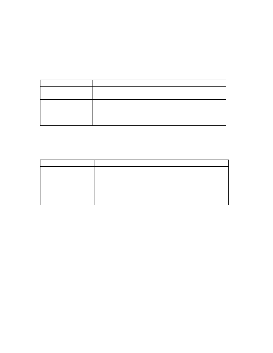
4.4.
THE MIPS INSTRUCTION SET
61
4.4.3.2
Jump
Op
Operands
Description
j
label
Jump to label lab.
jr
src1
Jump to location src1.
jal
label
Jump to label lab, and store the address of the next in-
struction in $ra.
jalr
src1
Jump to location src1, and store the address of the next
instruction in $ra.
4.4.4
Load, Store, and Data Movement
The second operand of all of the load and store instructions must be an address. The
MIPS architecture supports the following addressing modes:
Format
Meaning
◦ (reg)
Contents of reg.
◦ const
A constant address.
const(reg)
const + contents of reg.
◦ symbol
The address of symbol.
◦ symbol+const
The address of symbol + const.
◦ symbol+const(reg) The address of symbol + const + contents of reg.
4.4.4.1
Load
The load instructions, with the exceptions of li and lui, fetch a byte, halfword, or
word from memory and put it into a register. The li and lui instructions load a
constant into a register.
All load addresses must be aligned on the size of the item being loaded. For
example, all loads of halfwords must be from even addresses, and loads of words from
addresses cleanly divisible by four. The ulh and ulw instructions are provided to load
halfwords and words from addresses that might not be aligned properly.

62
CHAPTER 4.
THE MIPS R2000 INSTRUCTION SET
Op
Operands
Description
◦ la
des, addr
Load the address of a label.
lb(u)
des, addr
Load the byte at addr into des.
lh(u)
des, addr
Load the halfword at addr into des.
◦ li
des, const
Load the constant const into des.
lui
des, const
Load the constant const into the upper halfword of des,
and set the lower halfword of des to 0.
lw
des, addr
Load the word at addr into des.
lwl
des, addr
lwr
des, addr
◦ ulh(u)
des, addr
Load the halfword starting at the (possibly unaligned)
address addr into des.
◦ ulw
des, addr
Load the word starting at the (possibly unaligned) ad-
dress addr into des.
4.4.4.2
Store
The store instructions store a byte, halfword, or word from a register into memory.
Like the load instructions, all store addresses must be aligned on the size of the
item being stored. For example, all stores of halfwords must be from even addresses,
and loads of words from addresses cleanly divisible by four. The swl, swr, ush and
usw
instructions are provided to store halfwords and words to addresses which might
not be aligned properly.
Op
Operands
Description
sb
src1, addr
Store the lower byte of register src1 to addr.
sh
src1, addr
Store the lower halfword of register src1 to addr.
sw
src1, addr
Store the word in register src1 to addr.
swl
src1, addr
Store the upper halfword in src to the (possibly un-
aligned) address addr.
swr
src1, addr
Store the lower halfword in src to the (possibly unaligned)
address addr.
◦ ush
src1, addr
Store the lower halfword in src to the (possibly unaligned)
address addr.
◦ usw
src1, addr
Store the word in src to the (possibly unaligned) address
addr.
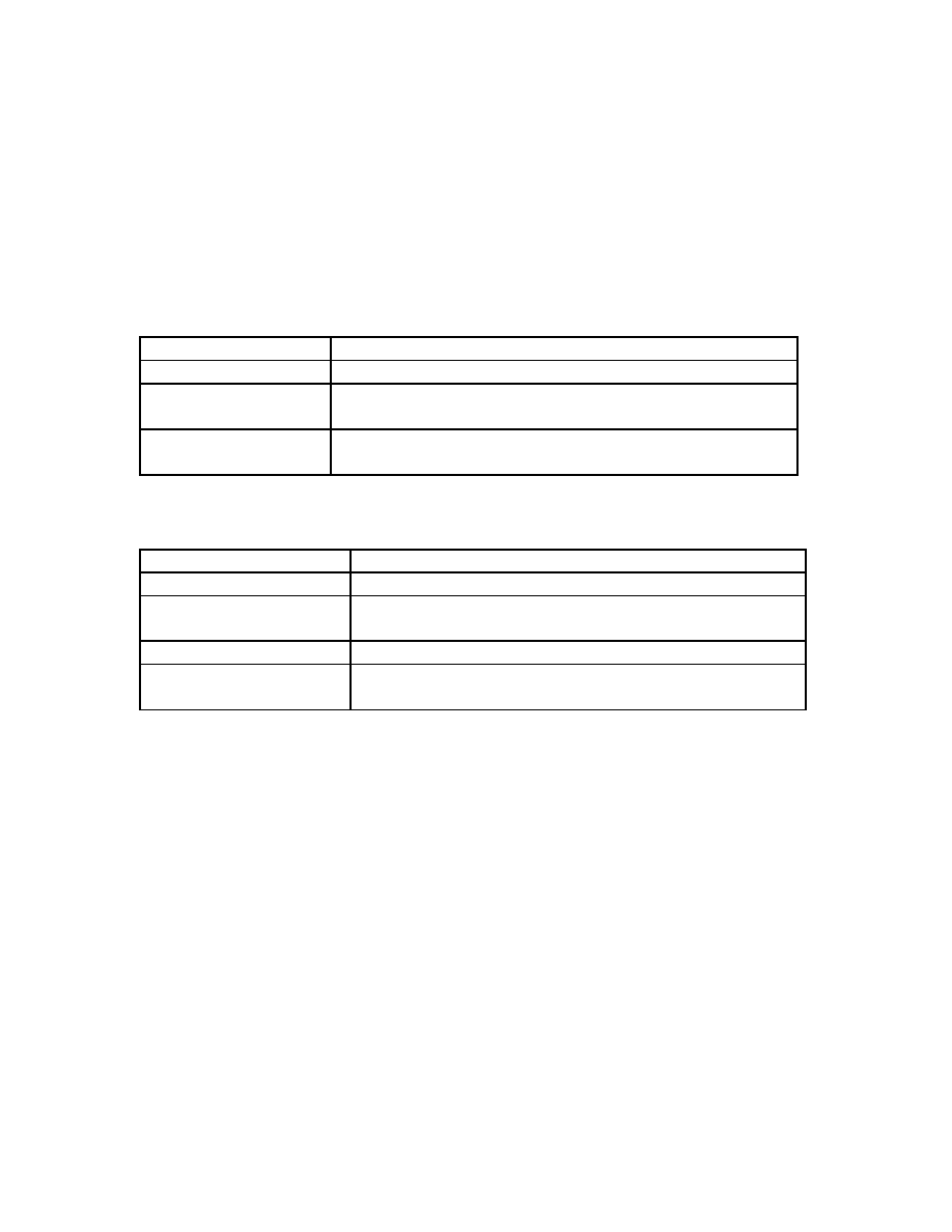
4.4.
THE MIPS INSTRUCTION SET
63
4.4.4.3
Data Movement
The data movement instructions move data among registers. Special instructions are
provided to move data in and out of special registers such as hi and lo.
Op
Operands
Description
◦ move
des, src1
Copy the contents of src1 to des.
mfhi
des
Copy the contents of the hi register to des.
mflo
des
Copy the contents of the lo register to des.
mthi
src1
Copy the contents of the src1 to hi.
mtlo
src1
Copy the contents of the src1 to lo.
4.4.5
Exception Handling
Op
Operands
Description
rfe
Return from exception.
syscall
Makes a system call. See 4.6.1 for a list of the SPIM
system calls.
break
const
Used by the debugger.
nop
An instruction which has no effect (other than taking a
cycle to execute).

64
CHAPTER 4.
THE MIPS R2000 INSTRUCTION SET
4.5
The SPIM Assembler
4.5.1
Segment and Linker Directives
Name
Parameters
Description
.data
addr
The following items are to be assembled into the data
segment. By default, begin at the next available address
in the data segment. If the optional argument addr is
present, then begin at addr.
.text
addr
The following items are to be assembled into the text
segment. By default, begin at the next available ad-
dress in the text segment. If the optional argument
addr is present, then begin at addr. In SPIM, the only
items that can be assembled into the text segment are
instructions and words (via the .word directive).
.kdata
addr
The kernel data segment. Like the data segment, but
used by the Operating System.
.ktext
addr
The kernel text segment. Like the text segment, but
used by the Operating System.
.extern
sym size
Declare as global the label sym, and declare that it is
size bytes in length (this information can be used by
the assembler).
.globl
sym
Declare as global the label sym.
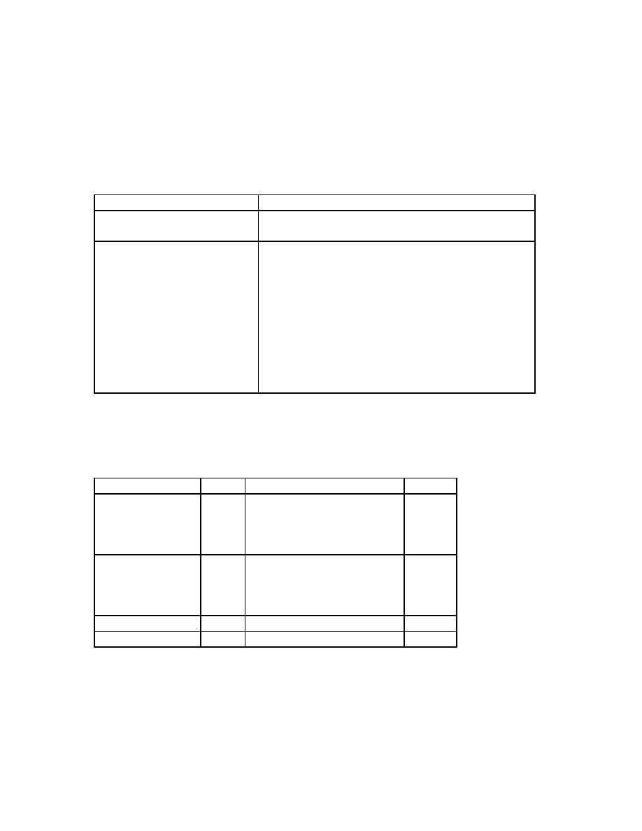
4.6.
THE SPIM ENVIRONMENT
65
4.5.2
Data Directives
Name
Parameters
Description
.align
n
Align the next item on the next 2
n
-byte boundary.
.align 0
turns off automatic alignment.
.ascii
str
Assemble the given string in memory. Do not null-
terminate.
.asciiz
str
Assemble the given string in memory. Do null-
terminate.
.byte
byte1 · · · byteN
Assemble the given bytes (8-bit integers).
.half
half1 · · · halfN
Assemble the given halfwords (16-bit integers).
.space
size
Allocate n bytes of space in the current seg-
ment. In SPIM, this is only permitted in the data
segment.
.word
word1 · · · wordN
Assemble the given words (32-bit integers).
4.6
The SPIM Environment
4.6.1
SPIM syscalls
Service
Code
Arguments
Result
print_int
1
$a0
none
print_float
2
$f12
none
print_double
3
$f12
none
print_string
4
$a0
none
read_int
5
none
$v0
read_float
6
none
$f0
read_double
7
none
$f0
read_string
8
$a0
(address), $a1 (length)
none
sbrk
9
$a0
(length)
$v0
exit
10
none
none
4.7
The Native MIPS Instruction Set
Many of the instructions listed here are not native MIPS instructions. Instead, they
are pseudoinstructions– macros that the assembler knows how to translate into native

66
CHAPTER 4.
THE MIPS R2000 INSTRUCTION SET
MIPS instructions. Instead of programming the “real” hardware, MIPS programmers
generally use the virtual machine implemented by the MIPS assembler, which is much
easier to program than the native machine.
For example, in most cases, the SPIM assembler will allow src2 to be a 32-bit
integer constant. Of course, since the MIPS instructions are all exactly 32 bits in
length, there’s no way that a 32-bit constant can fit in a 32-bit instruction word and
have any room left over to specify the operation and the operand registers! When
confronted with a 32-bit constant, the assembler uses a table of rules to generate a
sequence of native instructions that will do what the programmer has asked.
The assembler also performs some more intricate transformations to translate your
programs into a sequence of native MIPS instructions, but these will not be discussed
in this text.
By default, the SPIM environment implements the same virtual machine that the
MIPS assembler uses. It also implements the bare machine, if invoked with the -bare
option enabled.

4.8.
EXERCISES
67
4.8
Exercises
4.8.1
Many of the instructions available to the MIPS assembly language programmer are
not really instructions at all, but are translated by the assembler into one or more
instructions.
For example, the move instruction can be implemented using the add instruction.
Making use of register $0, which always contains the constant zero, and the fact that
the for any number x, x + 0 ≡ x, we can rewrite
move
des, src1
as
add
des, src1, $0
Similarly, since either the exclusive or or inclusive or of any number and 0 gives
the number, we could also write this as either of the following:
or
des, src1, $0
xor
des, src1, $0
Show how you could implement the following instructions, using other instructions
in the native MIPS instruction set:
1. rem des, src1, src2
2. mul des, src1, src2
3. li des, const
4. lui des, const
Keep in mind that the register $at is reserved for use by the assembler, so you
can feel free to use this register for scratch space. You must not clobber any other
registers, however.

68
CHAPTER 4.
THE MIPS R2000 INSTRUCTION SET

Chapter 5
MIPS Assembly Code Examples
by Daniel J. Ellard
The following sections include the source code for several of the programs referenced
by the tutorial. All of this source code is also available online.
For the convenience of the reader, the source code is listed here along with line
numbers in the left margin. These line numbers do not appear in the original code,
and it would be an error to include them in your own code.
69

70
CHAPTER 5.
MIPS ASSEMBLY CODE EXAMPLES
5.1
add2.asm
This program is described in section 2.4.
1
## Daniel J. Ellard -- 02/21/94
2
## add2.asm-- A program that computes and prints the sum
3
##
of two numbers specified at runtime by the user.
4
## Registers used:
5
##
$t0
- used to hold the first number.
6
##
$t1
- used to hold the second number.
7
##
$t2
- used to hold the sum of the $t1 and $t2.
8
##
$v0
- syscall parameter and return value.
9
##
$a0
- syscall parameter.
10
11
main:
12
## Get first number from user, put into $t0.
13
li
$v0, 5
# load syscall read_int into $v0.
14
syscall
# make the syscall.
15
move
$t0, $v0
# move the number read into $t0.
16
17
## Get second number from user, put into $t1.
18
li
$v0, 5
# load syscall read_int into $v0.
19
syscall
# make the syscall.
20
move
$t1, $v0
# move the number read into $t1.
21
22
add
$t2, $t0, $t1
# compute the sum.
23
24
## Print out $t2.
25
move
$a0, $t2
# move the number to print into $a0.
26
li
$v0, 1
# load syscall print_int into $v0.
27
syscall
# make the syscall.
28
29
li
$v0, 10
# syscall code 10 is for exit.
30
syscall
# make the syscall.
31
32
## end of add2.asm.

5.2.
HELLO.ASM
71
5.2
hello.asm
This program is described in section 2.5.
1
## Daniel J. Ellard -- 02/21/94
2
## hello.asm-- A "Hello World" program.
3
## Registers used:
4
##
$v0
- syscall parameter and return value.
5
##
$a0
- syscall parameter-- the string to print.
6
7
.text
8
main:
9
la
$a0, hello_msg
# load the addr of hello_msg into $a0.
10
li
$v0, 4
# 4 is the print_string syscall.
11
syscall
# do the syscall.
12
13
li
$v0, 10
# 10 is the exit syscall.
14
syscall
# do the syscall.
15
16
## Data for the program:
17
.data
18
hello_msg:
.asciiz "Hello World\n"
19
20
## end hello.asm

72
CHAPTER 5.
MIPS ASSEMBLY CODE EXAMPLES
5.3
multiples.asm
This program is described in section 2.7. The algorithm used is algorithm 2.1 (shown
on page 32).
1
## Daniel J. Ellard -- 02/21/94
2
## multiples.asm-- takes two numbers A and B, and prints out
3
##
all the multiples of A from A to A * B.
4
##
If B <= 0, then no multiples are printed.
5
## Registers used:
6
##
$t0
- used to hold A.
7
##
$t1
- used to hold B.
8
##
$t2
- used to store S, the sentinel value A * B.
9
##
$t3
- used to store m, the current multiple of A.
10
11
.text
12
main:
13
## read A into $t0, B into $t1.
14
li
$v0, 5
# syscall 5 = read_int
15
syscall
16
move
$t0, $v0
# A = integer just read
17
18
li
$v0, 5
# syscall 5 = read_int
19
syscall
20
move
$t1, $v0
# B = integer just read
21
22
blez
$t1, exit
# if B <= 0, exit.
23
24
mul
$t2, $t0, $t1
# S = A * B.
25
move
$t3, $t0
# m = A
26
27
loop:
28
move
$a0, $t3
# print m.
29
li
$v0, 1
# syscall 1 = print_int
30
syscall
# make the system call.
31
32
beq
$t2, $t3, endloop
# if m == S, we’re done.
33
add
$t3, $t3, $t0
# otherwise, m = m + A.
34
35
la
$a0, space
# print a space.
36
li
$v0, 4
# syscall 4 = print_string
37
syscall
38

5.3.
MULTIPLES.ASM
73
39
b
loop
# iterate.
40
endloop:
41
la
$a0, newline
# print a newline:
42
li
$v0, 4
# syscall 4 = print_string
43
syscall
44
45
exit:
# exit the program:
46
li
$v0, 10
# syscall 10 = exit
47
syscall
# we’re outta here.
48
49
## Here’s where the data for this program is stored:
50
.data
51
space:
.asciiz " "
52
newline:
.asciiz "\n"
53
54
## end of multiples.asm

74
CHAPTER 5.
MIPS ASSEMBLY CODE EXAMPLES
5.4
palindrome.asm
This program is described in section 2.8. The algorithm used is algorithm 2.2 (shown
on page 34).
1
## Daniel J. Ellard -- 02/21/94
2
## palindrome.asm -- read a line of text and test if it is a palindrome.
3
## Register usage:
4
##
$t1
- A.
5
##
$t2
- B.
6
##
$t3
- the character at address A.
7
##
$t4
- the character at address B.
8
##
$v0
- syscall parameter / return values.
9
##
$a0
- syscall parameters.
10
##
$a1
- syscall parameters.
11
12
.text
13
main:
# SPIM starts by jumping to main.
14
## read the string S:
15
la
$a0, string_space
16
li
$a1, 1024
17
li
$v0, 8
# load "read_string" code into $v0.
18
syscall
19
20
la
$t1, string_space
# A = S.
21
22
la
$t2, string_space
## we need to move B to the end
23
length_loop:
#
of the string:
24
lb
$t3, ($t2)
# load the byte at addr B into $t3.
25
beqz
$t3, end_length_loop
# if $t3 == 0, branch out of loop.
26
addu
$t2, $t2, 1
# otherwise, increment B,
27
b
length_loop
#
and repeat the loop.
28
end_length_loop:
29
subu
$t2, $t2, 2
## subtract 2 to move B back past
30
#
the ’\0’ and ’\n’.
31
test_loop:
32
bge
$t1, $t2, is_palin
# if A >= B, it’s a palindrome.
33
34
lb
$t3, ($t1)
# load the byte at addr A into $t3,
35
lb
$t4, ($t2)
# load the byte at addr B into $t4.
36
bne
$t3, $t4, not_palin
# if $t3 != $t4, not a palindrome.
37
# Otherwise,
38
addu
$t1, $t1, 1
#
increment A,

5.4.
PALINDROME.ASM
75
39
subu
$t2, $t2, 1
#
decrement B,
40
b
test_loop
#
and repeat the loop.
41
42
is_palin:
## print the is_palin_msg, and exit.
43
la
$a0, is_palin_msg
44
li
$v0, 4
45
syscall
46
b
exit
47
48
not_palin:
49
la
$a0, not_palin_msg
## print the is_palin_msg, and exit.
50
li
$v0, 4
51
syscall
52
b
exit
53
54
exit:
## exit the program:
55
li
$v0, 10
# load "exit" into $v0.
56
syscall
# make the system call.
57
58
## Here’s where the data for this program is stored:
59
.data
60
string_space:
.space
1024
# reserve 1024 bytes for the string.
61
is_palin_msg:
.asciiz "The string is a palindrome.\n"
62
not_palin_msg:
.asciiz "The string is not a palindrome.\n"
63
64
## end of palindrome.asm

76
CHAPTER 5.
MIPS ASSEMBLY CODE EXAMPLES
5.5
atoi-1.asm
This program is described in section 2.9.1. The algorithm used is algorithm 2.3 (shown
on page 37).
1
## Daniel J. Ellard -- 03/02/94
2
## atoi-1.asm -- reads a line of text, converts it to an integer, and
3
##
prints the integer.
4
## Register usage:
5
##
$t0
- S.
6
##
$t1
- the character pointed to by S.
7
##
$t2
- the current sum.
8
9
.text
10
main:
11
la
$a0, string_space
## read the string S:
12
li
$a1, 1024
13
li
$v0, 8
# load "read_string" code into $v0.
14
syscall
15
16
la
$t0, string_space
# Initialize S.
17
li
$t2, 0
# Initialize sum = 0.
18
19
sum_loop:
20
lb
$t1, ($t0)
# load the byte at addr S into $t1,
21
addu
$t0, $t0, 1
# and increment S.
22
23
## use 10 instead of ’\n’ due to SPIM bug!
24
beq
$t1, 10, end_sum_loop
# if $t1 == \n, branch out of loop.
25
26
mul
$t2, $t2, 10
# t2 *= 10.
27
28
sub
$t1, $t1, ’0’
# t1 -= ’0’.
29
add
$t2, $t2, $t1
# t2 += t1.
30
31
b
sum_loop
#
and repeat the loop.
32
end_sum_loop:
33
move
$a0, $t2
# print out the answer (t2).
34
li
$v0, 1
35
syscall
36
37
la
$a0, newline
# and then print out a newline.
38
li
$v0, 4

5.5.
ATOI-1.ASM
77
39
syscall
40
41
exit:
## exit the program:
42
li
$v0, 10
# load "exit" into $v0.
43
syscall
# make the system call.
44
45
.data
## Start of data declarations:
46
newline:
.asciiz "\n"
47
string_space:
.space
1024
# reserve 1024 bytes for the string.
48
49
## end of atoi-1.asm

78
CHAPTER 5.
MIPS ASSEMBLY CODE EXAMPLES
5.6
atoi-4.asm
This program is described in section 2.9.4. The algorithm used is algorithm 2.3 (shown
on page 37), modified as described in section 2.9.4.
1
## Daniel J. Ellard -- 03/04/94
2
## atoi-4.asm -- reads a line of text, converts it to an integer,
3
##
and prints the integer.
4
##
Handles signed numbers, detects bad characters, and overflow.
5
## Register usage:
6
##
$t0
- S.
7
##
$t1
- the character pointed to by S.
8
##
$t2
- the current sum.
9
##
$t3
- the "sign" of the sum.
10
##
$t4
- holds the constant 10.
11
##
$t5
- used to test for overflow.
12
.text
13
main:
14
la
$a0, string_space
# read the string S:
15
li
$a1, 1024
16
li
$v0, 8
# load "read_string" code into $v0.
17
syscall
18
19
la
$t0, string_space
# Initialize S.
20
li
$t2, 0
# Initialize sum = 0.
21
22
get_sign:
23
li
$t3, 1
# assume the sign is positive.
24
lb
$t1, ($t0)
# grab the "sign"
25
bne
$t1, ’-’, positive
# if not "-", do nothing.
26
li
$t3, -1
# otherwise, set t3 = -1, and
27
addu
$t0, $t0, 1
#
skip over the sign.
28
positive:
29
li
$t4, 10
# store the constant 10 in $t4.
30
sum_loop:
31
lb
$t1, ($t0)
# load the byte at addr S into $t1,
32
addu
$t0, $t0, 1
# and increment S,
33
34
## use 10 instead of ’\n’ due to SPIM bug!
35
beq
$t1, 10, end_sum_loop
# if $t1 == \n, branch out of loop.
36
37
blt
$t1, ’0’, end_sum_loop
# make sure 0 <= t1
38
bgt
$t1, ’9’, end_sum_loop
# make sure 9 >= t1

5.6.
ATOI-4.ASM
79
39
40
mult
$t2, $t4
# multiply $t2 by 10.
41
mfhi
$t5
# check for overflow;
42
bnez
$t5, overflow
#
if so, then report an overflow.
43
mflo
$t2
# get the result of the multiply
44
blt
$t2, $0, overflow
# make sure that it isn’t negative.
45
46
sub
$t1, $t1, ’0’
# t1 -= ’0’.
47
add
$t2, $t2, $t1
# t2 += t1.
48
blt
$t2, $0, overflow
49
50
b
sum_loop
#
and repeat the loop.
51
end_sum_loop:
52
mul
$t2, $t2, $t3
# set the sign properly.
53
54
move
$a0, $t2
# print out the answer (t2).
55
li
$v0, 1
56
syscall
57
58
la
$a0, newline
# and then print out a newline.
59
li
$v0, 4
60
syscall
61
62
b
exit
63
64
overflow:
# indicate that an overflow occurred.
65
la
$a0, overflow_msg
66
li
$v0, 4
67
syscall
68
b
exit
69
70
exit:
# exit the program:
71
li
$v0, 10
# load "exit" into $v0.
72
syscall
# make the system call.
73
74
.data
## Start of data declarations:
75
newline:
.asciiz "\n"
76
overflow_msg:
.asciiz "Overflow!\n"
77
string_space:
.space
1024
# reserve 1024 bytes for the string.
78
79
## end of atoi-4.asm

80
CHAPTER 5.
MIPS ASSEMBLY CODE EXAMPLES
5.7
printf.asm
Using syscalls for output can quickly become tedious, and output routines can quickly
muddy up even the neatest code, since it requires several assembly instructions just
to print out a number. To make matters worse, there is no syscall which prints out a
single ASCII character.
To help my own coding, I wrote the following printf function, which behaves
like a simplified form of the printf function in the standard C library. It implements
only a fraction of the functionality of the real printf, but enough to be useful. See
the comments in the code for more information.
1
## Daniel J. Ellard -- 03/13/94
2
## printf.asm--
3
##
an implementation of a simple printf work-alike.
4
5
## printf--
6
##
A simple printf-like function.
Understands just the basic forms
7
##
of the %s, %d, %c, and %% formats, and can only have 3 embedded
8
##
formats (so that all of the parameters are passed in registers).
9
##
If there are more than 3 embedded formats, all but the first 3 are
10
##
completely ignored (not even printed).
11
## Register Usage:
12
##
$a0,$s0 - pointer to format string
13
##
$a1,$s1 - format argument 1 (optional)
14
##
$a2,$s2 - format argument 2 (optional)
15
##
$a3,$s3 - format argument 3 (optional)
16
##
$s4
- count of formats processed.
17
##
$s5
- char at $s4.
18
##
$s6
- pointer to printf buffer
19
##
20
.text
21
.globl
printf
22
printf:
23
subu
$sp, $sp, 36
# set up the stack frame,
24
sw
$ra, 32($sp)
# saving the local environment.
25
sw
$fp, 28($sp)
26
sw
$s0, 24($sp)
27
sw
$s1, 20($sp)
28
sw
$s2, 16($sp)
29
sw
$s3, 12($sp)
30
sw
$s4, 8($sp)
31
sw
$s5, 4($sp)

5.7.
PRINTF.ASM
81
32
sw
$s6, 0($sp)
33
addu
$fp, $sp, 36
34
35
# grab the arguments:
36
move
$s0, $a0
# fmt string
37
move
$s1, $a1
# arg1 (optional)
38
move
$s2, $a2
# arg2 (optional)
39
move
$s3, $a3
# arg3 (optional)
40
41
li
$s4, 0
# set # of formats = 0
42
la
$s6, printf_buf
# set s6 = base of printf buffer.
43
44
printf_loop:
# process each character in the fmt:
45
lb
$s5, 0($s0)
# get the next character, and then
46
addu
$s0, $s0, 1
# bump up $s0 to the next character.
47
48
beq
$s5, ’%’, printf_fmt
# if the fmt character, then do fmt.
49
beq
$0, $s5, printf_end
# if zero, then go to end.
50
51
printf_putc:
52
sb
$s5, 0($s6)
# otherwise, just put this char
53
sb
$0, 1($s6)
# into the printf buffer,
54
move
$a0, $s6
# and then print it with the
55
li
$v0, 4
# print_str syscall
56
syscall
57
58
b
printf_loop
# loop on.
59
60
printf_fmt:
61
lb
$s5, 0($s0)
# see what the fmt character is,
62
addu
$s0, $s0, 1
# and bump up the pointer.
63
64
beq
$s4, 3, printf_loop
# if we’ve already processed 3 args,
65
# then *ignore* this fmt.
66
beq
$s5, ’d’, printf_int
# if ’d’, print as a decimal integer.
67
beq
$s5, ’s’, printf_str
# if ’s’, print as a string.
68
beq
$s5, ’c’, printf_char
# if ’c’, print as a ASCII char.
69
beq
$s5, ’%’, printf_perc
# if ’%’, print a ’%’
70
b
printf_loop
# otherwise, just continue.
71
72
printf_shift_args:
# shift over the fmt args,
73
move
$s1, $s2
# $s1 = $s2
74
move
$s2, $s3
# $s2 = $s3
75

82
CHAPTER 5.
MIPS ASSEMBLY CODE EXAMPLES
76
add
$s4, $s4, 1
# increment # of args processed.
77
78
b
printf_loop
# and continue the main loop.
79
80
printf_int:
# deal with a %d:
81
move
$a0, $s1
# do a print_int syscall of $s1.
82
li
$v0, 1
83
syscall
84
b
printf_shift_args
# branch to printf_shift_args
85
86
printf_str:
# deal with a %s:
87
move
$a0, $s1
# do a print_string syscall of $s1.
88
li
$v0, 4
89
syscall
90
b
printf_shift_args
# branch to printf_shift_args
91
92
printf_char:
# deal with a %c:
93
sb
$s1, 0($s6)
# fill the buffer in with byte $s1,
94
sb
$0, 1($s6)
# and then a null.
95
move
$a0, $s6
# and then do a print_str syscall
96
li
$v0, 4
#
on the buffer.
97
syscall
98
b
printf_shift_args
# branch to printf_shift_args
99
100
printf_perc:
# deal with a %%:
101
li
$s5, ’%’
# (this is redundant)
102
sb
$s5, 0($s6)
# fill the buffer in with byte %,
103
sb
$0, 1($s6)
# and then a null.
104
move
$a0, $s6
# and then do a print_str syscall
105
li
$v0, 4
#
on the buffer.
106
syscall
107
b
printf_loop
# branch to printf_loop
108
109
printf_end:
110
lw
$ra, 32($sp)
# restore the prior environment:
111
lw
$fp, 28($sp)
112
lw
$s0, 24($sp)
113
lw
$s1, 20($sp)
114
lw
$s2, 16($sp)
115
lw
$s3, 12($sp)
116
lw
$s4, 8($sp)
117
lw
$s5, 4($sp)
118
lw
$s6, 0($sp)
119
addu
$sp, $sp, 36
# release the stack frame.

5.7.
PRINTF.ASM
83
120
jr
$ra
# return.
121
122
.data
123
printf_buf:
.space
2
124
125
## end of printf.asm

84
CHAPTER 5.
MIPS ASSEMBLY CODE EXAMPLES
5.8
fib-o.asm
This program is described in section 3.1.1.3.
This is a (somewhat) optimized version of a program which computes Fibonacci
numbers. The optimization involves not building a stack frame unless absolutely
necessary. I wouldn’t recommend that you make a habit of optimizing your code in
this manner, but it can be a useful technique.
1
## Daniel J. Ellard -- 02/27/94
2
## fib-o.asm-- A program to compute Fibonacci numbers.
3
##
An optimized version of fib-t.asm.
4
## main--
5
## Registers used:
6
##
$v0
- syscall parameter and return value.
7
##
$a0
- syscall parameter-- the string to print.
8
.text
9
main:
10
subu
$sp, $sp, 32
# Set up main’s stack frame:
11
sw
$ra, 28($sp)
12
sw
$fp, 24($sp)
13
addu
$fp, $sp, 32
14
15
## Get n from the user, put into $a0.
16
li
$v0, 5
# load syscall read_int into $v0.
17
syscall
# make the syscall.
18
move
$a0, $v0
# move the number read into $a0.
19
jal
fib
# call fib.
20
21
move
$a0, $v0
22
li
$v0, 1
# load syscall print_int into $v0.
23
syscall
# make the syscall.
24
25
la
$a0, newline
26
li
$v0, 4
27
syscall
# make the syscall.
28
29
li
$v0, 10
# 10 is the exit syscall.
30
syscall
# do the syscall.
31
32
## fib-- (hacked-up caller-save method)
33
## Registers used:
34
##
$a0
- initially n.

5.8.
FIB-O.ASM
85
35
##
$t0
- parameter n.
36
##
$t1
- fib (n - 1).
37
##
$t2
- fib (n - 2).
38
.text
39
fib:
40
bgt
$a0, 1, fib_recurse
# if n < 2, then just return a 1,
41
li
$v0, 1
# don’t build a stack frame.
42
jr
$ra
43
# otherwise, set things up to handle
44
fib_recurse:
# the recursive case:
45
subu
$sp, $sp, 32
# frame size = 32, just because...
46
sw
$ra, 28($sp)
# preserve the Return Address.
47
sw
$fp, 24($sp)
# preserve the Frame Pointer.
48
addu
$fp, $sp, 32
# move Frame Pointer to new base.
49
50
move
$t0, $a0
# get n from caller.
51
52
# compute fib (n - 1):
53
sw
$t0, 20($sp)
# preserve n.
54
sub
$a0, $t0, 1
# compute fib (n - 1)
55
jal
fib
56
move
$t1, $v0
# t1 = fib (n - 1)
57
lw
$t0, 20($sp)
# restore n.
58
59
# compute fib (n - 2):
60
sw
$t1, 16($sp)
# preserve $t1.
61
sub
$a0, $t0, 2
# compute fib (n - 2)
62
jal
fib
63
move
$t2, $v0
# t2 = fib (n - 2)
64
lw
$t1, 16($sp)
# restore $t1.
65
66
add
$v0, $t1, $t2
# $v0 = fib (n - 1) + fib (n - 2)
67
lw
$ra, 28($sp)
# restore Return Address.
68
lw
$fp, 24($sp)
# restore Frame Pointer.
69
addu
$sp, $sp, 32
# restore Stack Pointer.
70
jr
$ra
# return.
71
72
## data for fib-o.asm:
73
.data
74
newline:
.asciiz "\n"
75
76
## end of fib-o.asm

86
CHAPTER 5.
MIPS ASSEMBLY CODE EXAMPLES
5.9
treesort.asm
This program is outlined in section 3.2. The treesort algorithm is given in algo-
rithm 3.1 (shown on page 51).
1
## Daniel J. Ellard -- 03/05/94
2
## tree-sort.asm -- some binary tree routines, in MIPS assembly.
3
##
4
##
The tree nodes are 3-word structures.
The first word is the
5
##
integer value of the node, and the second and third are the
6
##
left and right pointers.
7
##
&&&
NOTE-- the functions in this file assume this
8
##
&&&
representation!
9
10
## main --
11
##
1. Initialize the tree by creating a root node, using the
12
##
sentinel value as the value.
13
##
2. Loop, reading numbers from the user.
If the number is equal
14
##
to the sentinel value, break out of the loop; otherwise
15
##
insert the number into the tree (using tree_insert).
16
##
3. Print out the contents of the tree (skipping the root node),
17
##
by calling tree_print on the left and right
18
##
children of the root node.
19
## Register usage:
20
##
$s0
- the root of the tree.
21
##
$s1
- each number read in from the user.
22
##
$s2
- the sentinel value (right now, this is 0).
23
.text
24
main:
25
li
$s2, 0
# $s2 = the sentinel value.
26
27
## Step 1: create the root node.
28
## root = tree_node_create ($s2, 0, 0);
29
move
$a0, $s2
# val
= $s2
30
li
$a1, 0
# left
= NULL
31
li
$a2, 0
# right = NULL
32
jal
tree_node_create
# call tree_node_create
33
move
$s0, $v0
# and put the result into $s0.
34
35
36
## Step 2: read numbers and add them to the tree, until
37
## we see the sentinel value.
38
## register $s1 holds the number read.

5.9.
TREESORT.ASM
87
39
input_loop:
40
li
$v0, 5
# syscall 5 == read_int.
41
syscall
42
move
$s1, $v0
# $s1 = read_int
43
44
beq
$s1, $s2, end_input
# if we read the sentinel, break.
45
46
# tree_insert (number, root);
47
move
$a0, $s1
# number= $s1
48
move
$a1, $s0
# root
= $s0
49
jal
tree_insert
# call tree_insert.
50
51
b
input_loop
# repeat input loop.
52
end_input:
53
54
## Step 3: print out the left and right subtrees.
55
lw
$a0, 4($s0)
# print the root’s left child.
56
jal
tree_print
57
58
lw
$a0, 8($s0)
# print the root’s right child.
59
jal
tree_print
60
61
b
exit
# exit.
62
## end of main.
63
64
## tree_node_create (val, left, right): make a new node with the given
65
##
val and left and right descendants.
66
## Register usage:
67
##
$s0
- val
68
##
$s1
- left
69
##
$s2
- right
70
tree_node_create:
71
# set up the stack frame:
72
subu
$sp, $sp, 32
73
sw
$ra, 28($sp)
74
sw
$fp, 24($sp)
75
sw
$s0, 20($sp)
76
sw
$s1, 16($sp)
77
sw
$s2, 12($sp)
78
sw
$s3, 8($sp)
79
addu
$fp, $sp, 32
80
# grab the parameters:
81
move
$s0, $a0
# $s0 = val
82
move
$s1, $a1
# $s1 = left

88
CHAPTER 5.
MIPS ASSEMBLY CODE EXAMPLES
83
move
$s2, $a2
# $s2 = right
84
85
li
$a0, 12
# need 12 bytes for the new node.
86
li
$v0, 9
# sbrk is syscall 9.
87
syscall
88
move
$s3, $v0
89
90
beqz
$s3, out_of_memory
# are we out of memory?
91
92
sw
$s0, 0($s3)
# node->number
= number
93
sw
$s1, 4($s3)
# node->left
= left
94
sw
$s2, 8($s3)
# node->right
= right
95
96
move
$v0, $s3
# put return value into v0.
97
# release the stack frame:
98
lw
$ra, 28($sp)
# restore the Return Address.
99
lw
$fp, 24($sp)
# restore the Frame Pointer.
100
lw
$s0, 20($sp)
# restore $s0.
101
lw
$s1, 16($sp)
# restore $s1.
102
lw
$s2, 12($sp)
# restore $s2.
103
lw
$s3, 8($sp)
# restore $s3.
104
addu
$sp, $sp, 32
# restore the Stack Pointer.
105
jr
$ra
# return.
106
## end of tree_node_create.
107
108
## tree_insert (val, root): make a new node with the given val.
109
## Register usage:
110
##
$s0
- val
111
##
$s1
- root
112
##
$s2
- new_node
113
##
$s3
- root->val (root_val)
114
##
$s4
- scratch pointer (ptr).
115
tree_insert:
116
# set up the stack frame:
117
subu
$sp, $sp, 32
118
sw
$ra, 28($sp)
119
sw
$fp, 24($sp)
120
sw
$s0, 20($sp)
121
sw
$s1, 16($sp)
122
sw
$s2, 12($sp)
123
sw
$s3, 8($sp)
124
sw
$s3, 4($sp)
125
addu
$fp, $sp, 32
126

5.9.
TREESORT.ASM
89
127
# grab the parameters:
128
move
$s0, $a0
# $s0 = val
129
move
$s1, $a1
# $s1 = root
130
131
# make a new node:
132
# new_node = tree_node_create (val, 0, 0);
133
move
$a0, $s0
# val
= $s0
134
li
$a1, 0
# left
= 0
135
li
$a2, 0
# right = 0
136
jal
tree_node_create
# call tree_node_create
137
move
$s2, $v0
# save the result.
138
139
## search for the correct place to put the node.
140
## analogous to the following C code:
141
##
for (;;) {
142
##
root_val = root->val;
143
##
if (val <= root_val) {
144
##
ptr = root->left;
145
##
if (ptr != NULL) {
146
##
root = ptr;
147
##
continue;
148
##
}
149
##
else {
150
##
root->left = new_node;
151
##
break;
152
##
}
153
##
}
154
##
else {
155
##
/* the right side is symmetric. */
156
##
}
157
##
}
158
##
159
##
Commented with equivalent C code (you will lose many
160
##
style points if you ever write C like this...).
161
search_loop:
162
lw
$s3, 0($s1)
# root_val = root->val;
163
ble
$s0, $s3, go_left
# if (val <= s3) goto go_left;
164
b
go_right
# goto go_right;
165
166
go_left:
167
lw
$s4, 4($s1)
# ptr = root->left;
168
beqz
$s4, add_left
# if (ptr == 0) goto add_left;
169
move
$s1, $s4
# root = ptr;
170
b
search_loop
# goto search_loop;

90
CHAPTER 5.
MIPS ASSEMBLY CODE EXAMPLES
171
172
add_left:
173
sw
$s2, 4($s1)
# root->left = new_node;
174
b
end_search_loop
# goto end_search_loop;
175
176
go_right:
177
lw
$s4, 8($s1)
# ptr = root->right;
178
beqz
$s4, add_right
# if (ptr == 0) goto add_right;
179
move
$s1, $s4
# root = ptr;
180
b
search_loop
# goto search_loop;
181
182
add_right:
183
sw
$s2, 8($s1)
# root->right = new_node;
184
b
end_search_loop
# goto end_search_loop;
185
186
end_search_loop:
187
188
# release the stack frame:
189
lw
$ra, 28($sp)
# restore the Return Address.
190
lw
$fp, 24($sp)
# restore the Frame Pointer.
191
lw
$s0, 20($sp)
# restore $s0.
192
lw
$s1, 16($sp)
# restore $s1.
193
lw
$s2, 12($sp)
# restore $s2.
194
lw
$s3, 8($sp)
# restore $s3.
195
lw
$s4, 4($sp)
# restore $s4.
196
addu
$sp, $sp, 32
# restore the Stack Pointer.
197
jr
$ra
# return.
198
## end of node_create.
199
200
## tree_walk (tree):
201
##
Do an inorder traversal of the tree, printing out each value.
202
##
Equivalent C code:
203
##
void
tree_print (tree_t *tree)
204
##
{
205
##
if (tree != NULL) {
206
##
tree_print (tree->left);
207
##
printf ("%d\n", tree->val);
208
##
tree_print (tree->right);
209
##
}
210
##
}
211
## Register usage:
212
##
s0
- the tree.
213
tree_print:
214
# set up the stack frame:

5.9.
TREESORT.ASM
91
215
subu
$sp, $sp, 32
216
sw
$ra, 28($sp)
217
sw
$fp, 24($sp)
218
sw
$s0, 20($sp)
219
addu
$fp, $sp, 32
220
# grab the parameter:
221
move
$s0, $a0
# $s0 = tree
222
223
beqz
$s0, tree_print_end
# if tree == NULL, then return.
224
225
lw
$a0, 4($s0)
# recurse left.
226
jal
tree_print
227
228
# print the value of the node:
229
lw
$a0, 0($s0)
# print the value, and
230
li
$v0, 1
231
syscall
232
la
$a0, newline
# also print a newline.
233
li
$v0, 4
234
syscall
235
236
lw
$a0, 8($s0)
# recurse right.
237
jal
tree_print
238
239
tree_print_end:
# clean up and return:
240
lw
$ra, 28($sp)
# restore the Return Address.
241
lw
$fp, 24($sp)
# restore the Frame Pointer.
242
lw
$s0, 20($sp)
# restore $s0.
243
addu
$sp, $sp, 32
# restore the Stack Pointer.
244
jr
$ra
# return.
245
## end of tree_print.
246
247
248
## out_of_memory --
249
##
The routine to call when sbrk fails.
Jumps to exit.
250
out_of_memory:
251
la
$a0, out_of_mem_msg
252
li
$v0, 4
253
syscall
254
j
exit
255
## end of out_of_memory.
256
257
## exit --
258
##
The routine to call to exit the program.

92
CHAPTER 5.
MIPS ASSEMBLY CODE EXAMPLES
259
exit:
260
li
$v0, 10
# 10 is the exit syscall.
261
syscall
262
## end of program!
263
## end of exit.
264
265
## Here’s where the data for this program is stored:
266
.data
267
newline:
.asciiz "\n"
268
out_of_mem_msg: .asciiz "Out of memory!\n"
269
270
## end of tree-sort.asm
Wyszukiwarka
Podobne podstrony:
KM W assembly ENG stud mod
P000718 A Eng Vertical shaft assembly
M001882 B Eng Lower assembly
P000724 A Eng Lower assembly
P000720 D Eng Upper assembly
M001886 B Eng Lower assembly
P000729 D Eng Upper assembly
M001840 B Eng Oil tank assembly
P000726 A Eng Stem tube assembly
P000716 A Eng Pinion assembly
M001809 A Eng Vertical shaft assembly
M001791 B Eng Pinion assembly
P000720 C Eng Upper assembly
M001807 B Eng Propeller shaft assembly
M003913 A Eng Pinion shaft assembly
więcej podobnych podstron