Geometric and

Brightness Image

Interpolation

Professor

Valery Starovoitov

Digital Image Processing

Cyfrowe Przetwarzanie Obrazów

2

Geometric Transforms –

Whay?

• Geometric transforms permit the elimination of geometric

distortion that occurs when an image is captured.

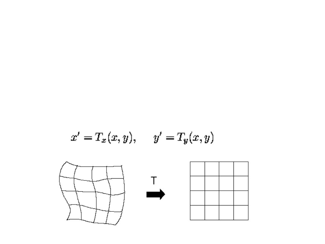
• A geometric transform is a vector function T that maps the

pixel (x,y) to a new position (x',y').

3

• The transformation equations are either known in advance

or

can be determined from known original and

transformed images.

• Several pixels in both images with known correspondence

are used to derive the unknown transformation.

• A geometric transform consists of two basic steps

:

1. Determin the pixel co-ordinate transform

 mapping of the co-ordinates of the input image pixel
to the point in the output image,

 the output point co-ordinates should be computed as
real numbers as the position does not necessarily match

the

digital grid after the transform.
2.

Find the point in the digital raster

which matches the

transformed point and determining its brightness.

Brightness is computed by interpolation of the

brightnesses of several points in the neighborhood.

4

Pixel co-ordinate

transforms

• It is a general case of finding the co-ordinates of a point

in the output image after a geometric transform.

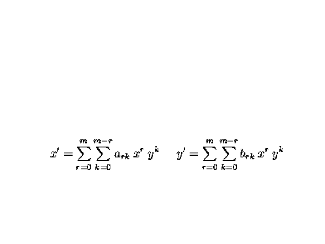
• Usually it is approximated by a polynomial equation.

5

• If pairs of corresponding points (x,y), (x',y') in both

images are known, it is possible to determine ark, brk

by solving a set of linear equations.

• More points than coefficients are usually used to get

robustness.

• If the geometric transform does not change rapidly

depending on position in the image, low order

approximating polynomials, m=2 or m=3, are used,

needing at least 6 or 10 pairs of corresponding points.

• The corresponding points should be distributed in the

image in a way that can express the geometric

transformation - usually they are spread uniformly.

• The higher the degree of the approximating

polynomial, the more sensitive to the distribution of

the pairs of corresponding points the geometric

transform.

6

•

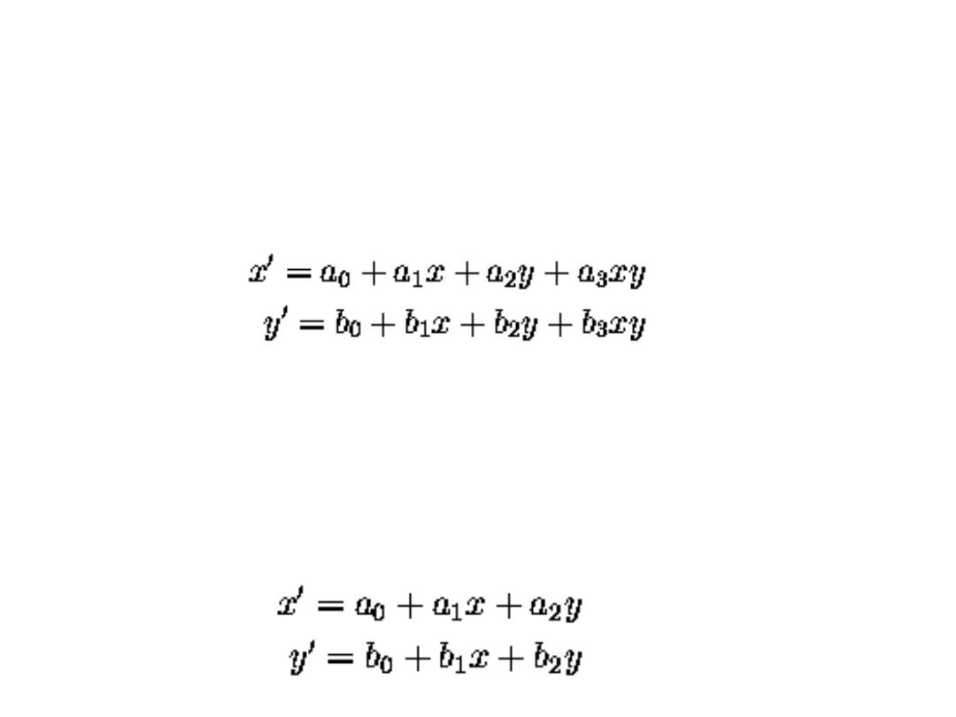
In practice, the geometric transform is often approximated
by the

bilinear transform

and

4 pairs

of corresponding

points are sufficient to find transform coefficients.

•

Simpler is the

affine transform

for which

3 pairs

of

corresponding points are sufficient to find the coefficients.

It includes rotation, translation, scaling and skewing.

7

More complex geometry?

In the case of complex geometric transforms do:

 approximation by

partitioning

an image into

smaller rectangular subimages;

 for each subimage, a simple geometric

transformation, such as the affine, is estimated
using pairs of corresponding pixels.

 simple geometric transform is then performed

separately in each subimage.

8

Brightness

interpolation

–

whay?

• After a planar image transformation the position of

a pixel does not

in general

fit the discrete raster

of the output image.

• Values on the integer grid are needed.

• Each pixel value in the output image raster can be

obtained by brightness interpolation of some
neighbors.

9

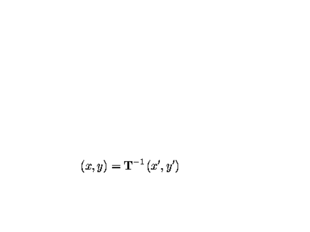
• The brightness interpolation problem is usually

expressed in a dual way

(by determining the brightness of the original point in

the input image that corresponds to the point in the

output image lying on the discrete raster).

• Computing the brightness value of the pixel (x',y') in the

output image where x' and y' lie on the discrete raster

10

•

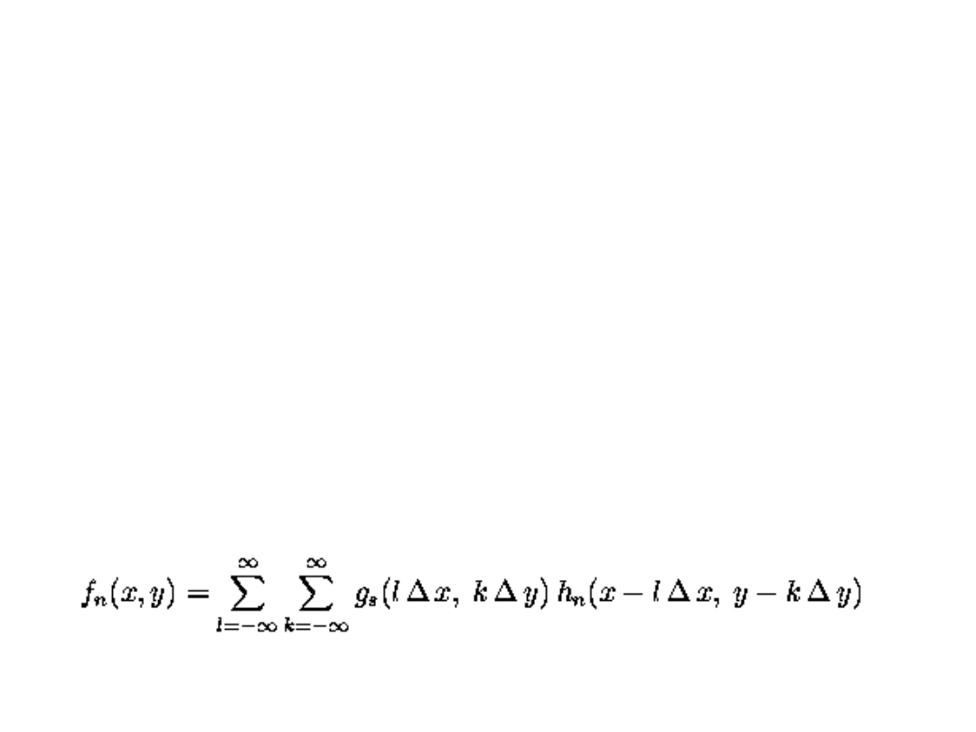
In general the real co-ordinates after inverse transformation
(dashed lines in Figures below) do not fit the input image
discrete raster (solid lines), and so brightness is not known.

•

To get the brightness value f of the point (x,y) the input
image is resampled.

fn(x,y) - result of interpolation
hn -

the interpolation kernel

Usually, a small neighborhood is used, outside which hn =

0.

11

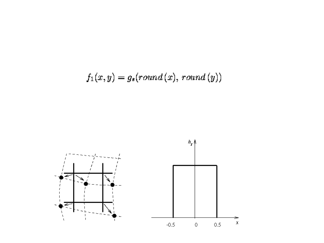
Nearest neighbor

interpolation

• We assign to the point (x,y) the brightness value of the nearest

point g in the discrete raster (the kernel contains

1 pixel

)

• The right side of Figure shows how the new brightness is

assigned. Dashed lines show how the inverse planar
transformation maps the raster of the output image into the
input image - full lines show the raster of the input image.

12

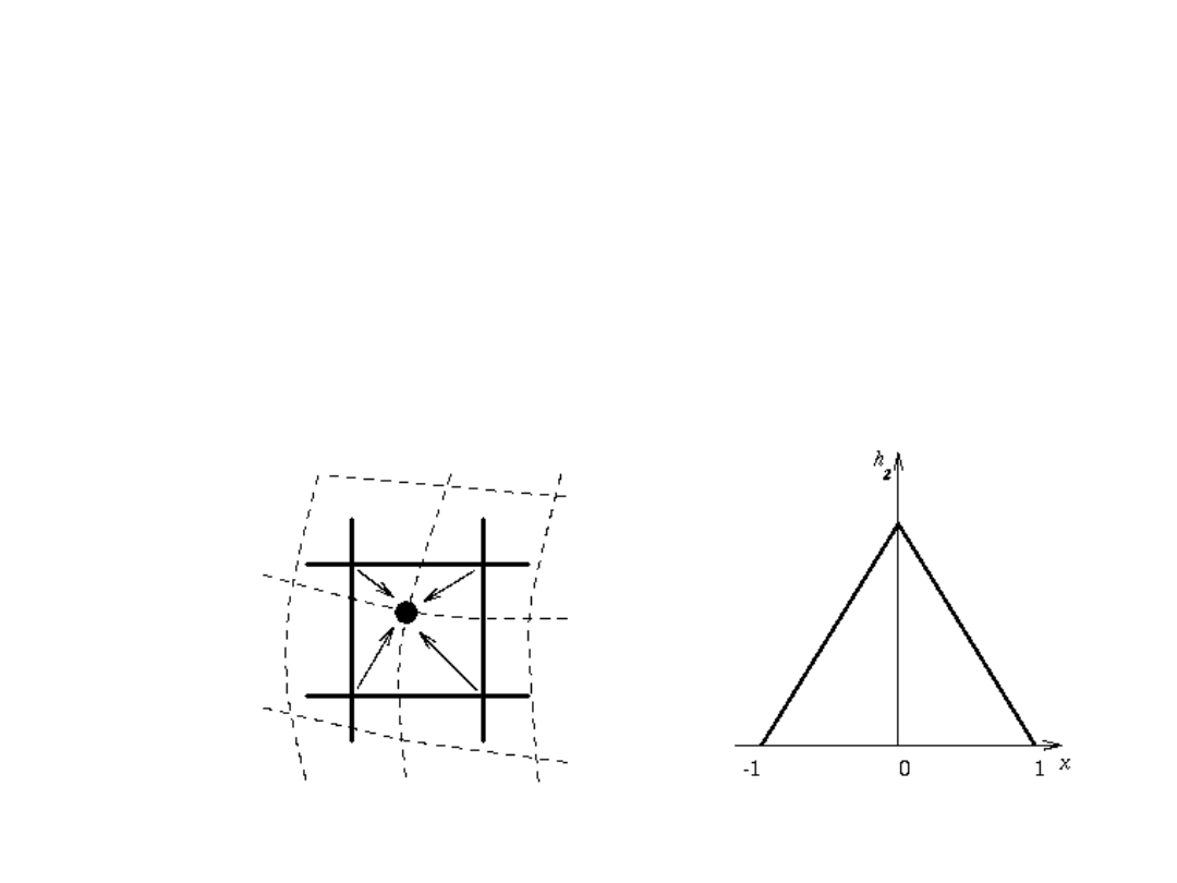
Bilinear interpolation

•

It explores four points neighboring the point (x,y), and
assumes that the brightness function is linear in this
neighborhood (the kernel contains 2x2=

4 pixels

).

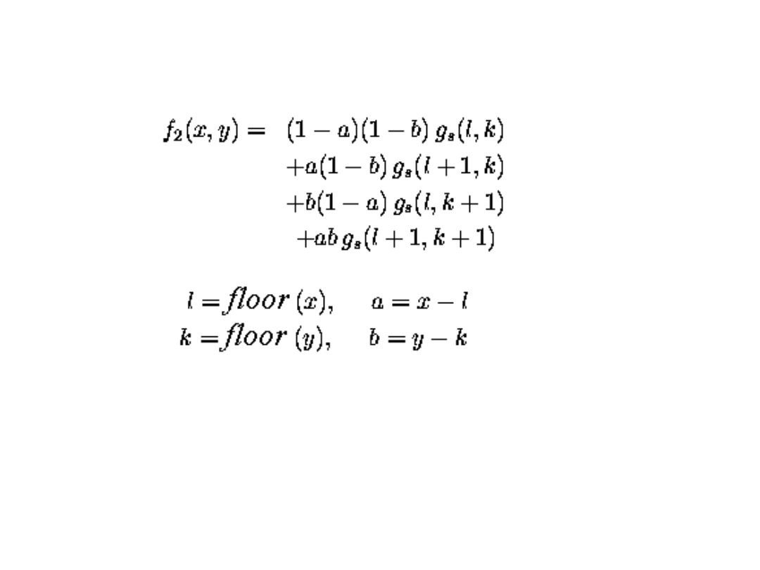
13

Linear interpolation is given by the equation

Linear interpolation can cause a small decrease in
resolution and blurring due to its averaging nature.

The problem of step like straight boundaries with the
nearest neighborhood interpolation is reduced.

14

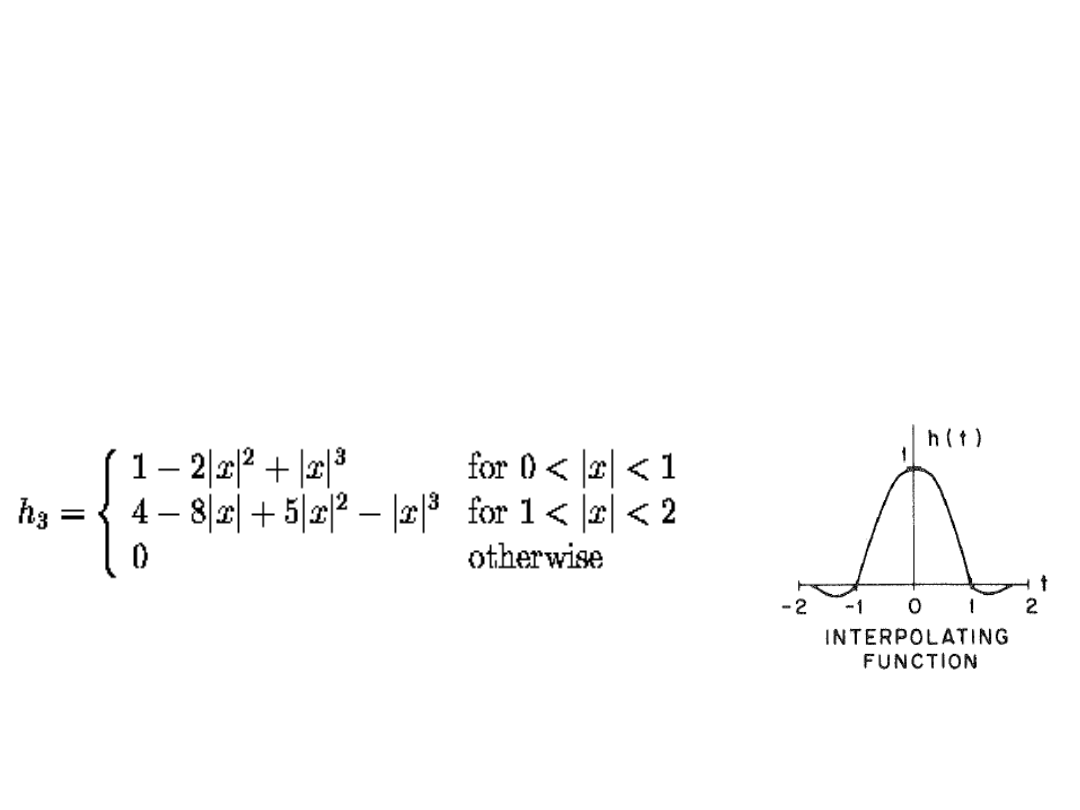
Bicubic interpolation

• It improves the model of the brightness function by

approximating it locally by a bicubic polynomial surface

(the kernel contains 4x4=

16 neighboring pixels

).

• Interpolation kernel (`Mexican hat') is given for x

15

• Bicubic interpolation does not suffer from the step-like

boundary problem of nearest neighborhood

interpolation, and copes with linear interpolation

blurring as well.

• Bicubic interpolation is often used in raster displays

that enable zooming with respect to an arbitrary point

-- if the nearest neighborhood method were used, areas

of the same brightness would increase.

• Bicubic interpolation preserves fine details in the image

very well, but has higher computational compelxity.

16

Image resized in 4 times by
nearest,
bilinear, and bicubic
interpolation

17

What to read?

 Milan Sonka, Image Pre-processing,

http://www.icaen.uiowa.edu/~dip/LECTURE/PreProcessing

2.html