Teaching Feynman’s sum-over-paths quantum theory

Edwin F. Taylor,

a

!

Stamatis Vokos,

b

!

and John M. O’Meara

c

!

Department of Physics, University of Washington, Seattle, Washington 98195-1560

Nora S. Thornber

d

!

Department of Mathematics, Raritan Valley Community College, Somerville, New Jersey 08876-1265

(Received 30 July 1997; accepted 25 November 1997)

We outline an introduction to quantum mechanics based on the sum-over-paths method originated
by Richard P. Feynman. Students use software with a graphics interface to model sums associated
with multiple paths for photons and electrons, leading to the concepts of electron wavefunction, the
propagator, bound states, and stationary states. Material in the first portion of this outline has been
tried with an audience of high-school science teachers. These students were enthusiastic about the
treatment, and we feel that it has promise for the education of physicists and other scientists, as
well as for distribution to a wider audience.

© 1998 American Institute of Physics.

@S0894-1866~98!01602-2#

Thirty-one years ago, Dick Feynman told me about his
‘‘sum over histories’’ version of quantum mechanics. ‘‘The
electron does anything it likes,’’ he said. ‘‘It just goes in
any direction at any speed, . . . however it likes, and then
you add up the amplitudes and it gives you the wave-
function.’’ I said to him, ‘‘You’re crazy.’’ But he wasn’t.

--Freeman Dyson, 1980

1

INTRODUCTION

The electron is a free spirit. The electron knows nothing of
the complicated postulates or partial differential equation of
nonrelativistic quantum mechanics. Physicists have known
for decades that the ‘‘wave theory’’ of quantum mechanics
is neither simple nor fundamental. Out of the study of
quantum electrodynamics

~QED! comes Nature’s simple,

fundamental three-word command to the electron: ‘‘Ex-
plore all paths.’’ The electron is so free-spirited that it re-
fuses to choose which path to follow—so it tries them all.
Nature’s succinct command not only leads to the results of
nonrelativistic quantum mechanics but also opens the door
to exploration of elementary interactions embodied in
QED.

Fifty years ago Richard Feynman

2

published the

theory of quantum mechanics generally known as ‘‘the path
integral method’’ or ‘‘the sum over histories method’’ or
‘‘the sum-over-paths method’’

~as we shall call it here!.

Thirty-three years ago Feynman wrote, with A. R. Hibbs,

3

a

more complete treatment in the form of a text suitable for
study at the upper undergraduate and graduate level. To-
ward the end of his career Feynman developed an elegant,
brief, yet completely honest, presentation in a popular book

written with Ralph Leighton.

4

Feynman did not use his

powerful sum-over-paths formulation in his own introduc-
tory text on quantum mechanics.

5

The sum-over-paths

method is sparsely represented in the physics-education
literature

6

and has not entered the mainstream of standard

undergraduate textbooks.

7

Why not? Probably because until

recently the student could not track the electron’s explora-
tion of alternative paths without employing complex math-
ematics. The basic idea is indeed simple, but its use and
application can be technically formidable. With current
desktop computers, however, a student can command the
modeled electron directly, pointing and clicking to select
paths for it to explore. The computer then mimics Nature to
sum the results for these alternative paths, in the process
displaying the strangeness of the quantum world. This use
of computers complements the mathematical approach used
by Feynman and Hibbs and often provides a deeper sense
of the phenomena involved.

This article describes for potential instructors the cur-

riculum for a new course on quantum mechanics, built
around a collection of software that implements Feynman’s
sum-over-paths formulation. The presentation begins with
the first half of Feynman’s popular QED book, which treats
the addition of quantum arrows for alternative photon paths
to analyze multiple reflections, single- and multiple-slit in-
terference, refraction, and the operation of lenses, followed
by introduction of the spacetime diagram and application of
the sum-over-paths theory to electrons. Our course then
leaves the treatment in Feynman’s book to develop the non-
relativistic wavefunction, the propagator, and bound states.
In a later section of this article we report on the response of
a small sample of students

~mostly high-school science

teachers

! to the first portion of this approach ~steps 1–11 in

the outline

!, tried for three semesters in an Internet com-

puter

conference

course

based

at

Montana

State

University.

8

a

!

Now at the Center for Innovation in Learning, Carnegie Mellon Univer-
sity, 4800 Forbes Ave., Pittsburgh, PA 15213; E-mail: [e-mail]

b

!

[e-mail]

c

!

[e-mail]

d

!

[e-mail]

190

COMPUTERS IN PHYSICS, VOL. 12, NO. 2, MAR/APR 1998

© 1998 AMERICAN INSTITUTE OF PHYSICS 0894-1866/98/12

~2!/190/10/$15.00

I. OUTLINE OF THE PRESENTATION

Below we describe the ‘‘logic line’’ of the presentation,
which takes as the fundamental question of quantum me-
chanics: Given that a particle is located at x

a

at time t

a

,

what is the probability that it will be located at x

b

at a later

time t

b

? We answer this question by tracking the rotating

hand of an imaginary quantum stopwatch as the particle
explores each possible path between the two events. The
entire course can be thought of as an elaboration of the
fruitful consequences of this single metaphor.

Almost every step in the following sequence is accom-

panied by draft software

9

with which the student explores

the logic of that step without using explicit mathematical
formalism. Only some of the available software is illus-
trated in the figures. The effects of spin are not included in
the present analysis.

A. The photon

Here are the steps in our presentation.

„1… Partial reflection of light: An everyday observa-

tion.

In his popular book QED, The Strange Theory of

Light and Matter, Feynman begins with the photon inter-
pretation of an everyday observation regarding light: partial
reflection of a stream of photons incident perpendicular to
the surface of a sheet of glass. Approximately 4% of inci-
dent photons reflect from the front surface of the glass and
another 4% from the back surface. For monochromatic
light incident on optically flat and parallel glass surfaces,
however, the net reflection from both surfaces taken to-
gether is typically not 8%. Instead, it varies from nearly 0%
to 16%, depending on the thickness of the glass. Classical
wave optics treats this as an interference effect.

„2… Partial reflection as sum over paths using quan-

tum stopwatches. The results of partial reflection can also
be correctly predicted by assuming that the photon explores
all paths between emitter and detector, paths that include
single and multiple reflections from each glass surface. The
hand of an imaginary ‘‘quantum stopwatch’’ rotates as the
photon explores each path.

10

Into the concept of this imagi-

nary stopwatch are compressed the fundamental strange-
ness and simplicity of quantum theory.

„3… Rotation rate for the hand of the photon quan-

tum stopwatch. How fast does the hand of the imaginary
photon quantum stopwatch rotate? Students recover all the
results of standard wave optics by assuming that it rotates
at the frequency of the corresponding classical wave.

11

„4… Predicting probability from the sum over paths.

The resulting arrow at the detector is the vector sum of the
final stopwatch hands for all alternative paths. The prob-
ability that the photon will be detected at a detector is pro-
portional to the square of the length of the resulting arrow
at that detector. This probability depends on the thickness
of the glass.

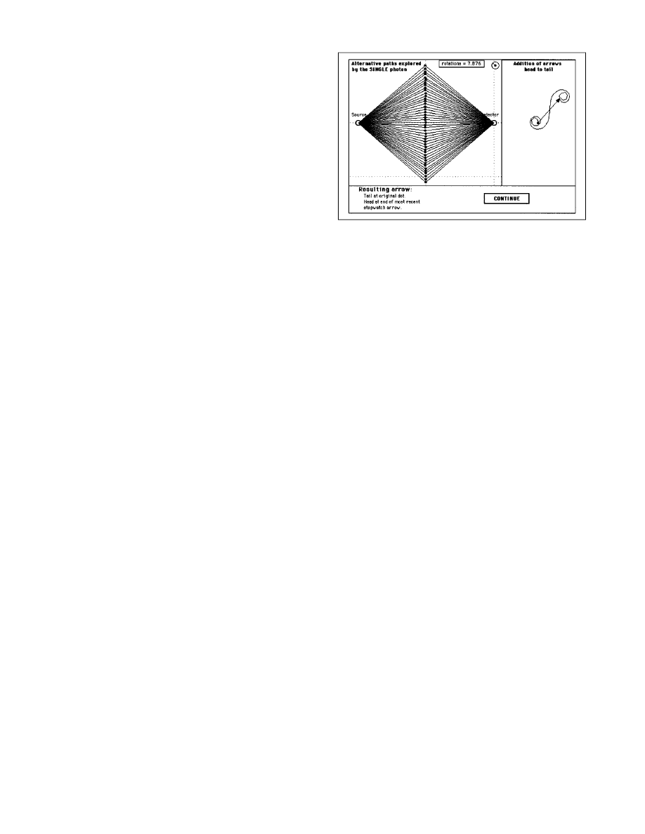
„5… Using the computer to sum selected paths for

the photon. Steps 1–4 embody the basic sum-over-paths
formulation. Figure 1 shows the computer interface for a
later task, in which the student selects paths in two space
dimensions between an emitter and a detector. The student
clicks with a mouse to place an intermediate point that
determines one of the paths between source and detector.
The computer then connects that point to source and detec-

tor, calculates rotation of the quantum stopwatch along the
path, and adds the small arrow from each path

~length

shown in the upper right corner of the left-hand panel

!

head-to-tail to arrows from all other selected paths to yield
the resulting arrow at the detector, shown at the right. The
figure in the right-hand panel approximates the Cornu spi-
ral. The resulting arrow is longer

12

than the initial arrow at

the emitter and is rotated approximately 45° with respect to
the arrow for the direct path. These properties of the Cornu
spiral are important in the later normalization of the arrow
that results from the sum over all paths between emitter and
detector

~step 16!.

B. The electron

„6… Goal: Find the rotation rate for the hand of the

electron quantum stopwatch.

The similarity between

electron interference and photon interference suggests that
the behavior of the electron may also be correctly predicted
by assuming that it explores all paths between emission and
detection.

~The remainder of this article will examine par-

ticle motion in only a single spatial dimension.

! As before,

exploration along each path is accompanied by the rotating
hand of an imaginary stopwatch. How rapidly does the
hand of the quantum stopwatch rotate for the electron? In
this case there is no obvious classical analog. Instead, we
prepare to answer the question by summarizing the classi-
cal mechanics of a single particle using the principle of
least action

~Fig. 2!.

„7… The classical principle of least action. Feynman

gives his own unique treatment of the classical principle of
least action in his book, The Feynman Lectures on
Physics.

13

A particle in a potential follows the path of least

action

~strictly speaking, extremal action! between the

events of launch and arrival. Action is defined as the time
integral of the quantity

~KE

2

PE

! along the path of the

particle, namely,

Figure 1. A single photon exploring alternative paths in two space dimen-
sions. The student clicks to choose intermediate points between source and
detector; the computer calculates the stopwatch rotation for each path and
adds the little arrows head-to-tail to yield the resulting arrow at the de-
tector, shown at the right.

COMPUTERS IN PHYSICS, VOL. 12, NO. 2, MAR/APR 1998

191

action

5S[

E

along the

worldline

~KE2PE!dt.

~1!

Here KE and PE are the kinetic and potential energies of
the particle, respectively. See Fig. 2.

This step introduces the spacetime diagram

~a plot of

the position of the stone as a function of time

!. Emission

and detection now become events, located in both space
and time on the spacetime diagram, and the idea of path
generalizes to that of the worldline that traces out on the
spacetime diagram the motion of the stone between these
endpoints. The expression for action is the first equation
required in the course.

„8… From the action comes the rotation rate of the

electron stopwatch. According to quantum theory,

14

the

number of rotations that the quantum stopwatch makes as
the particle explores a given path is equal to the action S
along that path divided by Planck’s constant h.

15

This fun-

damental

~and underived! postulate tells us that the fre-

quency f with which the electron stopwatch rotates as it
explores each path is given by the expression

16

f

5

KE

2PE

h

.

~2!

„9… Seamless transition between quantum and clas-

sical mechanics. In the absence of a potential

~Figs. 3 and

4

!, the major contributions to the resulting arrow at the

detector come from those worldlines along which the num-
ber of rotations differs by one-half rotation or less from that
of the classical path, the direct worldline

~Fig. 5!. Arrows

from all other paths differ greatly from one another in di-
rection and tend to cancel out. The greater the particle
mass, the more rapidly the quantum clock rotates

@for a

given speed in Eq.

~2!# and the nearer to the classical path

are those worldlines that contribute significantly to the final
arrow. In the limit of large mass, the only noncanceling
path is the single classical path of least action. Figures 3, 4,
and 5 illustrate the seamless transition between quantum
mechanics and classical mechanics in the sum-over-paths
approach.

C. The wavefunction

„10… Generalizing beyond emission and detection at

single events.

Thus far we have described an electron

emitted from a single initial event; we sample alternative
paths to construct a resulting arrow at a later event. But this
later event can be in one of several locations at a given later
time, and we can construct a resulting arrow for each of
these later events. This set of arrows appears along a single
horizontal ‘‘line of simultaneity’’ in a spacetime diagram,

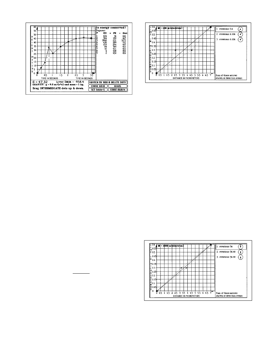
Figure 2. Computer display illustrating the classical principle of least
action for a 1-kg stone launched vertically near the Earth’s surface. A
trial worldline of the stone is shown on a spacetime diagram with the time
axis horizontal (as Feynman draws it in his introduction to action in Ref.
13). The student chooses points on the worldline and drags these points up
and down to find the minimum for the value of the action S, calculated by
the computer and displayed at the bottom of the screen. The table of
numbers on the right verifies (approximately) that energy is conserved for
the minimum-action worldline but is not conserved for segments 3 and 4,
which deviate from the minimum-action worldline.

Figure 3. Illustrating the ‘‘fuzziness’’ of worldlines around the classical
path for a hypothetical particle of mass 100 times that of the electron
moving in a region of zero potential. Worldlines are drawn on a spacetime
diagram with the time axis vertical (the conventional choice). The particle
is initially located at the event dot at the lower left and has a probability
of being located later at the event dot in the upper right. The three world-
lines shown span a pencil-shaped bundle of worldlines along which the
stopwatch rotations differ by half a revolution or less from that of the
straight-line classical path. This pencil of worldlines makes the major
contribution to the resulting arrow at the detector (Fig. 5).

Figure 4. Reduced ‘‘fuzziness’’ of the pencil of worldlines around the
classical path for a particle of mass 1000 times that of the electron (10
times the mass of the particle whose motion is pictured in Fig. 3). Both
this and Fig. 3 illustrate the seamless transition between quantum and
classical mechanics provided by the sum-over-paths formulation.

192

COMPUTERS IN PHYSICS, VOL. 12, NO. 2, MAR/APR 1998

as shown in Fig. 6. In Fig. 6 the emission event is at the
lower left and a finite packet is formed by selecting a short
sequence of the arrows along the line of simultaneity at
time 5.5 units. A later row of arrows

~shown at time 11.6

units

! can be constructed from the earlier set of arrows by

the usual method of summing the final stopwatch arrows
along paths connecting each point on the wavefunction at
the earlier time to each point on the wavefunction at the
later time. In carrying out this propagation from the earlier
to the later row of dots, details of the original single emis-
sion event

~in the lower left of Fig. 6! need no longer be

known.

In Figs. 6 and 7 the computer calculates and draws

each arrow in the upper row

~time near 12 units in both

figures

! by simple vector addition of every arrow

propagated/rotated from the lower row

~time 5.5 units in

Fig. 6, time 3 units in Fig. 7

!. Each such propagation/

rotation takes place only along the SINGLE direct world-
line between the initial point and the detection point—NOT
along ALL worldlines between each lower and each upper
event, as required by the sum-over-paths formulation. Typi-
cally students do not notice this simplification. Steps 12–16
repair this omission, but to look ahead we remark that for a
free particle the simpler

~and incomplete! formulation illus-

trated in Fig. 7 still approximates the correct relative prob-
abilities of finding the particle at different places at the later
time.

„11… The wavefunction as a discrete set of arrows.

We give the name

~nonrelativistic! wavefunction to the col-

lection of arrows that represent the electron at various
points in space at a given time. In analogy to the intensity
in wave optics, the probability of finding the electron at a
given time and place is proportional to the squared magni-
tude of the arrow at that time and place. We can now in-
vestigate the propagation forward in time of an arbitrary
initial wavefunction

~Fig. 7!. The sum-over-paths proce-

dure uses the initial wavefunction to predict the wavefunc-
tion at a later time.

Representing a continuous wavefunction with a finite

series of equally spaced arrows can lead to computational
errors, most of which are avoidable or can be made insig-
nificant for pedagogic purposes.

18

The process of sampling alternative paths

~steps 1–11

and their elaboration

! has revealed essential features of

quantum mechanics and provides a self-contained, largely
nonmathematical introduction to the subject for those who
do not need to use quantum mechanics professionally. This
has been tried with students, with the results described later
in this article. The following steps are the result of a year’s
thought about how to extend the approach to include cor-
rectly ALL paths between emission and detection.

D. The propagator

„12… Goal: Sum ALL paths using the ‘‘propaga-

tor.’’ Thus far we have been sampling alternative paths

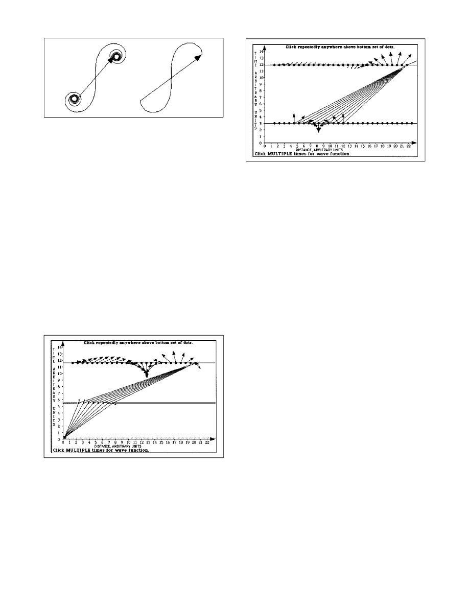
Figure 5. Addition of arrows for alternative paths, as begun in Fig. 1. The
resulting arrow for a (nearly) complete Cornu spiral (left) is approxi-
mated (right) by contributions from only those worldlines along which the
number of rotations differs by one-half rotation or less from that of the
direct worldline. This approximation is used in Figs. 3 and 4 and in our
later normalization process (step 16 below).

Figure 6. The concept of ‘‘wavefunction’’ arises from the application of
the sum-over-paths formulation to a particle at two sequential times. The
student clicks at the lower left to create the emission event, clicks to select
the endpoints of an intermediate finite packet of arrows, then clicks once
above these to choose a later time. The computer samples worldlines from
the emission (whose initial stopwatch arrow is assumed to be vertical)
through the intermediate packet, constructing a later series of arrows at
possible detection events along the upper line. We call this series of ar-
rows at a given time the ‘‘wavefunction.’’ This final wavefunction can be
derived from the arrows in the intermediate packet, without considering
the original emission (Ref. 17).

Figure 7. An extended arbitrary initial wavefunction now has a life of its
own, with the sum-over-paths formulation telling it how to propagate for-
ward in time. Here a packet moves to the right.

COMPUTERS IN PHYSICS, VOL. 12, NO. 2, MAR/APR 1998

193

between emitter and detector. Figures 1, 3, and 4 imply the
use of only a few alternative paths between a single emis-
sion event and a single detection event. Each arrow in the
final wavefunction of Fig. 7 sums the contributions along
just a single straight worldline from each arrow in the ini-
tial wavefunction. But Nature tells the electron

~in the cor-

rected form of our command

!: Explore ALL worldlines. To

draw Fig. 7 correctly we need to take into account propa-
gation along ALL worldlines—including those that zigzag
back and forth in space—between every initial dot on the
earlier wavefunction and each final dot on the later wave-
function. If Nature is good to us, there will be a simple
function that summarizes the all-paths result. This function
accepts as input the arrow at a single initial dot on the
earlier wavefunction and delivers as output the correspond-
ing arrow at a single dot on the later wavefunction due to
propagation via ALL intermediate worldlines. If it exists,
this function answers the fundamental question of quantum
mechanics: Given that a particle is located at x

a

at time t

a

,

what is the probability

~derived from the squared magni-

tude of the resulting arrow

! that it will be located at x

b

at a

later time t

b

? It turns out that Nature is indeed good to us;

such a function exists. The modern name for this function
is the ‘‘propagator,’’ the name we adopt here because the
function tells how a quantum arrow propagates from one
event to a later event. The function is sometimes called the
‘‘transition function’’; Feynman and Hibbs call it the ‘‘ker-
nel,’’ leading to the symbol K in the word equation

S

arrow at

later event b

D

5K~b,a!

S

arrow at

earlier event a

D

.

~3!

The propagator K(b,a) in Eq.

~3! changes the magni-

tude and direction of the initial arrow at event a to create
the later arrow at event b via propagation along ALL
worldlines. This contrasts with the method used to draw
Fig. 7, in which each contribution to a resulting upper ar-
row is constructed by rotating an arrow from the initial
wavefunction along the SINGLE direct worldline only. In
what follows, we derive the propagator by correcting the
inadequacies in the construction of Fig. 7, but for a simpler
initial wavefunction.

„13… Demand that a uniform wavefunction stay uni-

form. We derive the free-particle propagator heuristically
by demanding that an initial wavefunction uniform in space
propagate forward in time without change.

19

The initial

wavefunction, the central portion of which is shown at the
bottom of Fig. 8, is composed of vertical arrows of equal
length. The equality of the squared magnitudes of these
arrows implies an initial probability distribution uniform in
x. Because of the very wide extent of this initial wavefunc-
tion along the x direction, we expect that any diffusion of
probability will leave local probability near the center con-
stant for a long time. This analysis does not tell us that the
arrows will also stay vertical with time, but we postulate
this result as well.

20

The student applies a trial propagator

function between every dot in the initial wavefunction and
every dot in the final wavefunction, modifying the propa-
gator until the wavefunction does not change with time, as
shown in Fig. 10.

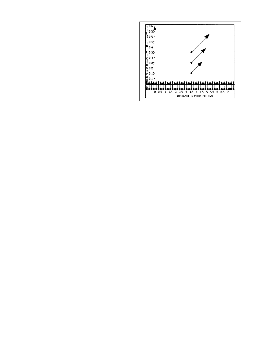
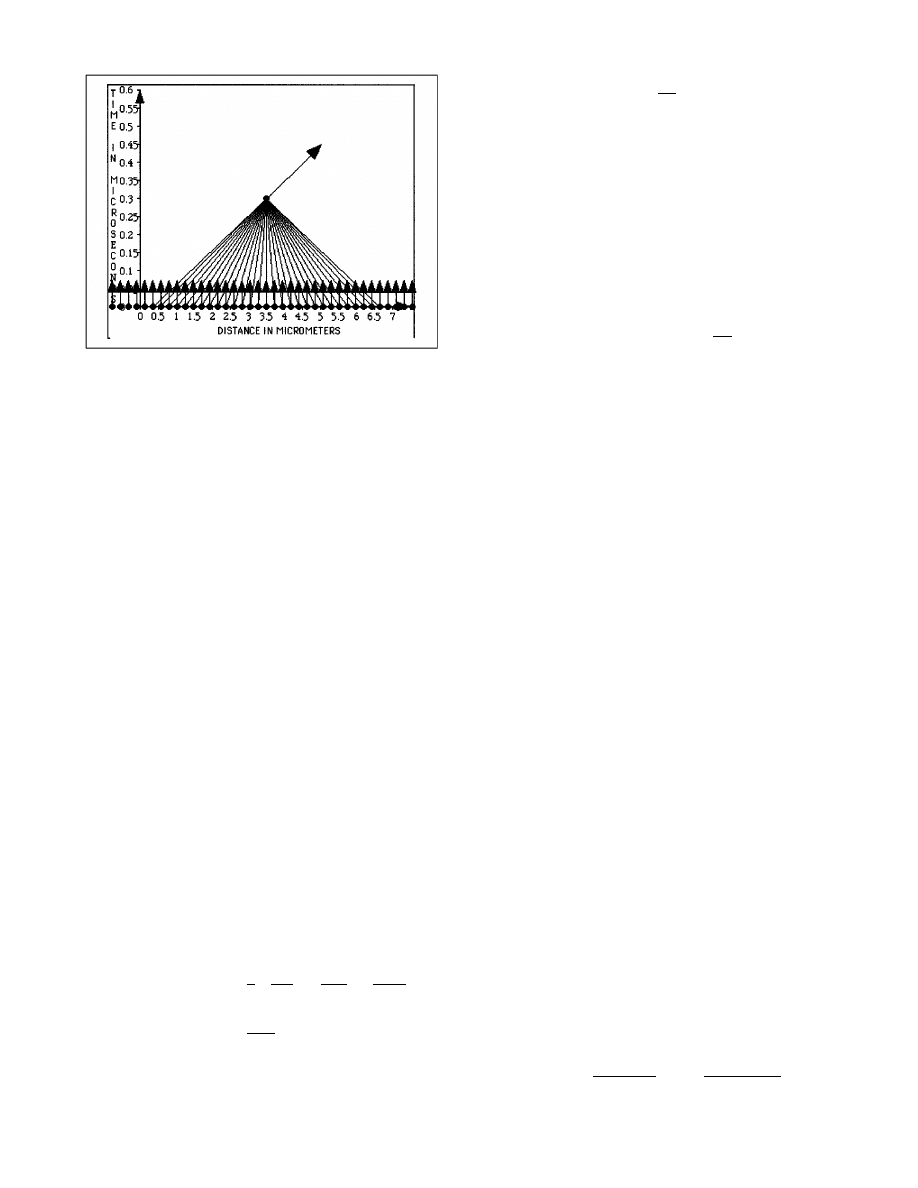
„14… Errors introduced by sampling paths. In Fig.

8, we turn the computer loose, asking it to construct single

arrows at three later times from an initially uniform wave-
function shown along the bottom. The computer derives
each later arrow incorrectly by propagating/rotating the
contribution from each lower arrow along a SINGLE direct
worldline, then summing the results from all these direct
worldlines, as it did in constructing Fig. 7. The resulting
arrows at three later times are shown in Fig. 8 at one-fifth
their actual lengths. These lengths are much too great to
represent a wavefunction that does not change with time.
This is the first lack shown by these resulting arrows. The
second is that they do not point upward as required. The
reason for this net rotation can be found in the Cornu spiral

~Fig. 5!, which predicts the same net rotation for all later
times. The third deficiency is that the resulting arrows in-
crease in length with time. All of these deficiencies spring
from the failure of the computer program to properly sum
the results over ALL paths

~all worldlines! between each

initial arrow and the final arrow. We will now correct these
insufficiencies to construct the free-particle propagator.

„15… Predicting the properties of the propagator.

From a packaged list, the student chooses

~and may

modify

! a trial propagator function. The computer then ap-

plies it to EACH arrow in the initial wavefunction of Fig. 8
as this arrow influences the resulting arrow at the single
detection event later in time, then sums the results for all
initial arrows. What can we predict about the properties of
this propagator function?

~a! By trial and error, the student will find that the propa-

gator must include an initial angle of minus 45° in
order to cancel the rotation of the resultant arrow
shown in Fig. 8.

~b! We assume that the rotation rate in space and time for

Figure 8. Resulting arrows at different times, derived naively from an
initial wavefunction that is uniform in profile and very wide along the x
axis (extending in both directions beyond the segment shown as parallel
arrows at the bottom of the screen). The resulting arrows at three later
times, shown at one-fifth of their actual lengths, are each calculated by
rotating every initial arrow along the single direct worldline connecting it
with the detection event and summing the results. The resulting arrows are
(1) too long, (2) point in the wrong direction, and (3) incorrectly increase
in length with time.

194

COMPUTERS IN PHYSICS, VOL. 12, NO. 2, MAR/APR 1998

the trial free-particle propagator is given by frequency
Eq.

~2! with PE equal to zero, applied along the direct

worldline.

~c! The propagator must have a magnitude that decreases

with time to counteract the time increase in magni-
tude displayed in Fig. 8.

„16… Predicting the magnitude of the propagator.

The following argument leads to a trial value for the mag-
nitude of the propagator: Figs. 3–5 suggest that most of the
contributions to the arrow at the detector come from world-
lines along which the quantum stopwatch rotation differs
by half a revolution or less from that of the direct world-
line. A similar argument leads us to assume that the major
influence that the initial wavefunction has at the detection
event results from those initial arrows, each of which ex-
ecutes one-half rotation or less along the direct worldline to
the detection event. The ‘‘pyramid’’ in Fig. 9 displays
those worldlines that satisfy this criterion.

@The vertical

worldline to the apex of this pyramid corresponds to zero
particle velocity, so zero kinetic energy, and therefore zero
net rotation according to Eq.

~2!.#

Let X be the half-width of the base of the pyramid

shown in Fig. 9, and let T be the time between the initial
wavefunction and the detection event. Then Eq.

~2! yields

an expression that relates these quantities to the assumed
one-half rotation of the stopwatch along the pyramid’s
slanting right-hand worldline, namely,

number of rotations

5

1

2

5

KE

h

T

5

m

v

2

2h

T

5

mX

2

2hT

2

T

5

mX

2

2hT

.

~4!

Solving for 2X, we find the width of the pyramid base

in Fig. 9 to be

2X

52

S

hT

m

D

1/2

.

~5!

The arrows in the initial wavefunction that contribute sig-
nificantly to the resulting arrow at the detection event lie
along the base of this pyramid. The number of these arrows
is proportional to the width of this base. To correct the
magnitude of the resulting arrow, then, we divide by this
width and insert a constant of proportionality B. The con-
stant B allows for the arbitrary spacing of the initial arrows

~spacing chosen by the student! and provides a correction
to our rough estimate. The resulting normalization constant
for the magnitude of the resulting arrow at the detector is

S

normalization

constant for

magnitude of

resulting arrow

D

5B

S

m

hT

D

1/2

.

~6!

The square-root expression on the right-side of Eq.

~6!

has the units of inverse length. In applying the normaliza-
tion, we multiply it by the spatial separation between adja-
cent arrows in the wavefunction.

The student determines the value of the dimensionless

constant B by trial and error, as described in the following
step.

„17… Heuristic derivation of the free-particle propa-

gator. Using an interactive computer program, the student
tries a propagator that gives each initial arrow a twist of

245°, then rotates it along the direct worldline at a rate
computed using Eq.

~2! with PE50. The computer applies

this trial propagator for the time T to EVERY spatial sepa-
ration between EACH arrow in the initial wavefunction and
the desired detection event, summing these contributions to
yield a resulting arrow at the detection event. The computer
multiplies the magnitude of the resulting arrow at the de-
tector by the normalization constant given in Eq.

~6!. The

student then checks that for a uniform initial wavefunction
the resulting arrow points in the same direction as the initial
arrows. Next the student varies the value of the constant B
in Eq.

~6! until the resulting arrow has the same length as

each initial arrow,

21

thereby discovering that B

51. ~Nature

is very good to us.

! The student continues to use the com-

puter to verify this procedure for different time intervals T
and different particle masses m, and to construct wavefunc-
tions

~many detection events! at several later times from the

initial wavefunction

~Fig. 10!.

„18… Mathematical form of the propagator. The

summation carried out between all the arrows in the initial
wavefunction and each single detection event approximates
the integral in which the propagator function K is usually
employed

22

for a continuous wavefunction,

c

~x

b

,t

b

!5

E

2`

1`

K

~b,a!

c

~x

a

,t

a

!dx

a

.

~7!

Here the label a refers to a point in the initial wavefunc-
tion, while the label b applies to a point on a later wave-
function. The free-particle propagator K is usually written

23

K

~b,a!5

S

m

ih

~t

b

2t

a

!

D

1/2

exp

im

~x

b

2x

a

!

2

2

\~t

b

2t

a

!

,

~8!

Figure 9. Similar to Fig. 8. Here the ‘‘pyramid’’ indicates those direct
worldlines from the initial wavefunction to the detection event for which
the number of rotations of the quantum stopwatch differs by one-half
revolution or less compared with that of the shortest (vertical) worldline.
(The central vertical worldline implies zero rotation.)

COMPUTERS IN PHYSICS, VOL. 12, NO. 2, MAR/APR 1998

195

where the conventional direction of rotation is counter-
clockwise, zero angle being at a rightward orientation of
the arrow. Notice the difference between h in the normal-
ization constant and

\ in the exponent. The square-root

coefficient on the right side of this equation embodies not
only the normalization constant of Eq.

~6! but also the ini-

tial twist of

245°, expressed in the quantity i

21/2

. This

coefficient is not a function of x, so it ‘‘passes through’’
the integral of Eq.

~7! and can be thought of as normalizing

the summation as a whole. Students may or may not be
given Eqs.

~7! and ~8! at the discretion of the instructor.

The physical content has been made explicit anyway, and
the computer will now generate consequences as the stu-
dent directs.

E. Propagation in time of a nonuniform wavefunction

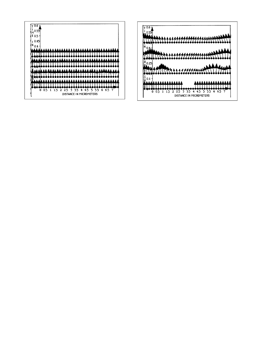
„19… Time development of the wavefunction. With

a verified free-particle propagator, the student can now pre-
dict the time development of any initial one-dimensional
free-particle wavefunction by having the computer apply
this propagator to all arrows in the initial wavefunction to
create each arrow in the wavefunction at later times. Figure
11 shows an example of such a change with time.

„20… Moving toward the Schro¨dinger equation.

Students can be encouraged to notice that an initial wave-
function very wide in extent with a ramp profile

~constant

slope, i.e., constant first x derivative

! propagates forward in

time without change. We can then challenge the student to
construct for a free particle an initial wavefunction of finite
extent in the x direction that does not change with time.
Attempting this impossible task is instructive. Why is the
task impossible? Because the profile of an initial wavefunc-
tion finite in extent necessarily includes changes in slope,

that is, a second x derivative. The stage is now set for
development of the Schro¨dinger equation, which relates the
time derivative of a free-particle wavefunction to its second
space derivative. We do not pursue this development in the
present article.

24

F. Wavefunction in a potential

„21… Time development in the presence of a poten-

tial. Equation

~2! describes the rotation rate of the quan-

tum stopwatch when a potential is present. A constant po-
tential uniform in space simply changes everywhere the
rotation rate of the quantum clock hand, as the student can
verify from the display. Expressions for propagators in
various potentials, such as the infinitely deep square well
and the simple harmonic oscillator potential, have been de-
rived by specialists.

25

It is too much to ask students to

search out these more complicated propagators by trial and
error. Instead, such propagators are simply built into the
computer program and the student uses them to explore the
consequences for the time development of the wavefunc-
tion.

G. Bound states and stationary states

„22… Bound states. Once the propagator for a one-

dimensional binding potential has been programmed into
the computer, the student can investigate how any wave-
function develops with time in that potential. Typically, the
probability peaks slosh back and forth with time. Now we
can again challenge the student to find wavefunctions that
do not change with time

~aside from a possible overall ro-

tation

!. One or two examples provided for a given potential

prove the existence of these stationary states, challenging
the student to construct others for the same potential. The
student will discover that for each stationary state all ar-
rows of the wavefunction rotate in unison, and that the

Figure 10. Propagation of an initially uniform wavefunction of very wide
spatial extent (a portion shown in the bottom row of arrows) forward to
various later times (upper three rows of arrows), using the correct free-
particle propagator to calculate the arrow at each later point from all of
the arrows in the initial wavefunction. The student chooses the wavefunc-
tion in the bottom row, then clicks once above the bottom row for each
later time. The computer then uses the propagator to construct the new
wavefunction.

Figure 11. Time propagation of an initial wavefunction with a ‘‘hole’’ in
it, using the verified free-particle propagator. The student chooses the
initial wavefunction and clicks once for each later time. The computer
then uses the correct free-particle propagator to propagate the initial
wavefunction forward to this later time, showing that the ‘‘hole’’ spreads
outward.

196

COMPUTERS IN PHYSICS, VOL. 12, NO. 2, MAR/APR 1998

more probability peaks the stationary-state wavefunction
has, the more rapid is this unison rotation. This leads to
discrete energies as a characteristic of stationary states.

Spin must be added as a separate consideration in this

treatment, as it must in all conventional introductions to
nonrelativistic quantum mechanics.

II. EARLY TRIALS AND STUDENT RESPONSE

For three semesters, fall and spring of the academic year
1995–96 and fall of 1996, Feynman’s popular QED book
was the basis of an online-computer-conference college
course called ‘‘Demystifying Quantum Mechanics,’’ taken
by small groups of mostly high-school science teachers.
The course covered steps 1–11 that were described earlier.
The computer-conference format is described elsewhere.

26

Students used early draft software to interact with Fey-

nman’s sum-over-paths model to enrich their class discus-
sions and to solve homework exercises.

Because the computer displays and analyzes paths ex-

plored by the particle, no equations are required for the first
third of the semester. Yet, from the very first week, discus-
sions showed students to be deeply engaged in fundamental
questions about quantum mechanics. Moreover, the soft-
ware made students accountable in detail: exercises could
be completed only by properly using the software.

How did students respond to the sum-over-paths for-

mulation? Listen to comments of students enrolled in the
fall 1995 course.

~Three periods separate comments by dif-

ferent students.

!

‘‘The reading was incredible . . . I really get a
kick out of Feynman’s totally off-wall way of
describing

this

stuff . . . Truly

a

ground-

breaker! . . . He brings up some REALLY in-
teresting ideas that I am excited to discuss with
the rest of the class . . . I’m learning twice as
much as I ever hoped to, and we have just
scratched the surface . . . It’s all so profound. I
find myself understanding ‘physics’ at a more
fundamental level . . . I enjoy reading him be-
cause he seems so honest about what he

~and

everyone else

! does not know . . . Man, it made

me feel good to read that Feynman couldn’t
understand this stuff either . . . it occurs to me
that the reading is easy because of the software
simulations we have run . . . the software plays
a very strong role in helping us understand the
points being made by Feynman.’’

During the spring 1996 semester, a student remarked

in a postscript:

‘‘PS—Kudos for this course. I got an A in my
intro qm class without having even a fraction of
the understanding I have now . . . This all
makes so much more sense now, and I owe a
large part of that to the software. I never

@had#

such compelling and elucidating simulations in
my former course. Thanks again!!!’’

At the end of the spring 1996 class, participants com-

pleted an evaluative questionnaire. There were no substan-
tial negative comments.

27

Feynman’s treatment and the

software were almost equally popular:

Q5. I found Feynman’s approach to quantum mechanics to
be

boring/irritating

1

2

3

4

5

fascinating/
stimulating

student choices:

0

0

0

2

11

~average: 4.85!.

Q18. For my understanding of the material, the software
was

not important

1

2

3

4

5 very important

student choices:

0

0

1

1

11

~average: 4.77!.

Student enthusiasm encourages us to continue the de-

velopment of this approach to quantum mechanics. We rec-
ognize, of course, that student enthusiasm may be gratify-
ing, but it does not tell us in any detail what they have
learned. We have not tested comprehensively what students
understand after using this draft material, or what new mis-
conceptions it may have introduced into their mental pic-
ture of quantum mechanics. Indeed, we will not have a
basis for setting criteria for testing student mastery of the
subject until our ‘‘story line’’ and accompanying software
are further developed.

28

III. ADVANTAGES AND DISADVANTAGES OF THE SUM-OVER-PATHS
FORMULATION

The advantages of introducing quantum mechanics using
the sum-over-paths formulation include the following.

~i!

The basic idea is simple, easy to visualize, and
quickly executed by computer.

~ii!

The sum-over-paths formulation begins with a free
particle moving from place to place, a natural exten-
sion of motions studied in classical mechanics.

~iii!

The process of sampling alternative paths

~steps

1–11 and their elaboration

! reveals essential features

of quantum mechanics and can provide a self-
contained, largely nonmathematical introduction to
the subject for those who do not need to use quan-
tum mechanics professionally.

~iv!

Summing all paths with the propagator permits nu-
merically accurate results of free-particle motion
and bound states

~steps 12–22!.

~v!

One can move seamlessly back and forth between
classical and quantum mechanics

~see Figs. 3 and 4!.

~vi!

Paradoxically, although little mathematical formal-
ism is required to introduce the sum-over-paths for-
mulation, it leads naturally to important mathemati-
cal tools used in more advanced physics. ‘‘Feynman
diagrams,’’ part of an upper undergraduate or gradu-
ate course, can be thought of as extensions of the
meaning of ‘‘paths.’’

29

The propagator is actually an

example of a Green’s function, useful throughout
theoretical physics, as are variational methods

30

in-

cluding the method of stationary phase. When
formalism is introduced later, the propagator in
Dirac

notation

has

a

simple

form:

K(b,a)

5

^

x

b

,t

b

ux

a

,t

a

&

.

The major disadvantages of introducing quantum me-

chanics using the sum-over-paths formulation include the
following.

COMPUTERS IN PHYSICS, VOL. 12, NO. 2, MAR/APR 1998

197

~i!

It is awkward in analyzing bound states in arbitrary
potentials. Propagators in analytic form have been
worked out for only simple one-dimensional binding
potentials.

~ii!

Many instructors are not acquainted with teaching
the sum-over-paths formulation, so they will need to
expend more time and effort in adopting it.

~iii!

It requires more time to reach analysis of bound
states.

IV. SOME CONCLUSIONS FOR TEACHING QUANTUM MECHANICS

The sum-over-paths formulation

~steps 1–11! allows physi-

cists to present quantum mechanics to the entire intellectual
community at a fundamental level with minimum manipu-
lation of equations.

The enthusiasm of high-school science teachers par-

ticipating in the computer conference courses tells us that
the material is motivating for those who have already had
contact with basic notions of quantum mechanics.

The full sum-over-paths formulation

~steps 1–22!

does not fit conveniently into the present introductory treat-
ments of quantum mechanics for the physics major. It con-
stitutes a long introduction before derivation of the Schro¨-
dinger equation. We consider this incompatibility to be a
major advantage; the attractiveness of the sum-over-paths
formulation should force reexamination of the entire intro-
ductory quantum sequence.

ACKNOWLEDGMENTS

Portions of this article were adapted from earlier writing in
collaboration with Paul Horwitz, who has also given much
advice on the approach and on the software. Philip Morri-
son encouraged the project. Lowell Brown and Ken
Johnson have given advice and helped guard against errors
in the treatment

~not always successfully!!. A. P. French,

David Griffiths, Jon Ogborn, and Daniel Styer offered use-
ful critiques of the article. Detailed comments on an earlier
draft were provided also by Larry Sorensen and by students
in his class at the University of Washington: Kelly Barry,
Jeffery Broderick, David Cameron, Matthew Carson,
Christopher Cross, David DeBruyne, James Enright, Robert
Jaeger, Kerry Kimes, Shaun Leach, Mark Mendez, and Dev
Sen. One of the authors

~E.F.T.! would like to thank the

members of the Physics Education Group for their hospi-
tality during the academic year 1996–97. In addition, the
authors would like to thank Lillian C. McDermott and the
other members of the Physics Education Group, especially
Bradley S. Ambrose, Paula R. L. Heron, Chris Kautz,
Rachel E. Scherr, and Peter S. Shaffer for providing them
with valuable feedback. The article was significantly im-
proved following suggestions from David M. Cook, an As-
sociate Editor of this journal. This work was supported in
part by NSF Grant No. DUE-9354501, which includes sup-
port from the Division of Undergraduate Education, other
Divisions of EHR, and the Physics Division of MPS.

REFERENCES

1. F. Dyson, in Some Strangeness in the Proportion, edited by H. Woolf

~Addison–Wesley, Reading, MA, 1980!, p. 376.

2. R. P. Feynman, Rev. Mod. Phys. 20, 367

~1948!.

3. R. P. Feynman and A. R. Hibbs, Quantum Mechanics and Path Inte-

grals

~McGraw–Hill, New York, 1965!.

4. R. P. Feynman, QED, The Strange Theory of Light and Matter

~Prin-

ceton University Press, Princeton, 1985

!.

5. R. P. Feynman, R. B. Leighton, and M. Sands, The Feynman Lectures

on Physics

~Addison–Wesley, Reading, MA, 1964!, Vol. III.

6. See, for example, N. J. Dowrick, Eur. J. Phys. 18, 75

~1997!. Titles of

articles on this subject in the Am. J. Phys. may be retrieved online at
http://www.amherst.edu/

;ajp.

7. R. Shankar, Principles of Quantum Mechanics, 2nd ed.

~Plenum, New

York, 1994

!. This text includes a nice introduction of the sum-over-

paths theory and many applications, suitable for an upper undergradu-
ate or graduate course.

8. For a description of the National Teachers Enhancement Network at

Montana State University and a listing of current courses, see the Web
site http://www.montana.edu//wwwxs.

9. Draft software written by Taylor in the computer language cT.

For a description of this language, see the Web site http://
cil.andrew.cum.edu/ct.html.

10. To conform to the ‘‘stopwatch’’ picture, rotation is taken to be clock-

wise, starting with the stopwatch hand straight up. We assume that
later

@for example, with Eq. ~8! in step 18# this convention will be

‘‘professionalized’’ to the standard counterclockwise rotation, starting
with initial orientation in the rightward direction. The choice of either
convention, consistently applied, has no effect on probabilities calcu-
lated using the theory.

11. Feynman explains later in his popular QED book

~page 104 of Ref. 4!

that the photon stopwatch hand does not rotate while the photon is in
transit. Rather, the little arrows summed at the detection event arise
from a series of worldlines originating from a ‘‘rotating’’ source.

12. In Fig. 1, the computer simply adds up stopwatch-hand arrows for a

sampling of alternative paths in two spatial dimensions. The resulting
arrow at the detector is longer than the original arrow at the emitter.
Yet the probability of detection

~proportional to the square of the

length of the arrow at the detector

! cannot be greater than unity.

Students do not seem to worry about this at the present stage in the
argument.

13. R. P. Feynman, R. B. Leighton, and M. Sands, The Feynman Lectures

on Physics

~Addison–Wesley, Reading, MA, 1964!, Vol. II, Chap. 19.

14. See, Ref. 2, Sec. 4, postulate II.
15. The classical principle of least action assumes fixed initial and final

events. This is exactly what the sum-over-paths formulation of quan-
tum mechanics needs also, with fixed events of emission and detec-
tion. The classical principle of least action is valid only when dissi-
pative forces

~such as friction! are absent. This condition is also

satisfied by quantum mechanics, since there are no dissipative forces
at the atomic level.

16. A naive reading of Eq.

~2! seems to be inconsistent with the deBroglie

relation when one makes the substitutions f

5v/l5p/(ml) and KE

5p

2

/(2m) and PE

50. In Ref. 3, pp. 44–45, Feynman and Hibbs

resolve this apparent inconsistency, which reflects the difference be-
tween group velocity and phase velocity of a wave.

17. See a similar figure in Ref. 3, Fig. 3-3, p. 48.
18. We have found three kinds of errors that result from representing a

continuous wavefunction with a finite series of equally spaced arrows.
~1! Representing a wavefunction of wide x extension with a narrower
width of arrows along the x direction leads to propagation of edge
effects into the body of the wavefunction. The region near the center
changes a negligible amount if the elapsed time is sufficiently short.
~2! The use of discrete arrows can result in a Cornu spiral that does
not complete its inward scroll to the theoretically predicted point at
each end. For example, in the Cornu spiral in the left-hand panel of
Fig. 5, the use of discrete arrows leads to repeating small circles at
each end, rather than convergence to a point. The overall resulting
arrow

~from the tail of the first little arrow to the head of the final

arrow

! can differ slightly in length from the length it would have if the

scrolls at both ends wound to their centers. The fractional error is
typically reduced by increasing the number of arrows, thereby in-
creasing the ratio of resulting arrow length to the length of the little

198

COMPUTERS IN PHYSICS, VOL. 12, NO. 2, MAR/APR 1998

component arrows.

~3! The formation of a smooth Cornu spiral at the

detection event requires that the difference in rotation to a point on the
final wavefunction be small between arrows that are adjacent in the
original wavefunction. But for very short times between the initial and
later wavefunctions, some of the connecting worldlines are nearly
horizontal in spacetime diagrams similar to Figs. 3 and 4, correspond-
ing to large values of kinetic energy KE, and therefore high rotation
frequency f

5KE/h. Under such circumstances, the difference in ro-

tation at an event on the final wavefunction can be great between
arrows from adjacent points in the initial wavefunction. This may lead
to distortion of the Cornu spiral or even its destruction. In summary, a
finite series of equally spaced arrows can adequately represent a con-
tinuous wavefunction provided the number of arrows

~for a given total

x extension

! is large and the time after the initial wavefunction is

neither too small nor too great. We have done a preliminary quanti-
tative analysis of these effects showing that errors can be less than 2%
for a total number of arrows easily handled by desktop computers.
This accuracy is adequate for teaching purposes.

19. In Ref. 3, p. 42ff, Feynman and Hibbs carry out a complicated inte-

gration to find the propagator for a free electron. However, the nor-
malization constant used in their integration is determined only later
in their treatment

~Ref. 3, p. 78! in the course of deriving the Schro¨-

dinger equation.

20. This is verified by the usual Schro¨dinger analysis. The initial free-

particle wavefunction shown in Figs. 8–10 has zero second x deriva-
tive, so it will also have a zero time derivative.

21. We add a linear taper to each end of the initial wavefunctions used in

constructing Figs. 8–11 to suppress ‘‘high-frequency components’’
that otherwise appear along the entire length of a later wavefunction
when a finite initial wavefunction has a sharp space termination. The
tapered portions lie outside the views shown in these figures.

22. In Ref. 3, Eq.

~3-42!, p. 57.

23. In Ref. 3, Eq.

~3-3!, p. 42.

24. In Refs. 2 and 3; see also D. Derbes, Am. J. Phys. 64, 881

~1996!.

25. In Ref. 3; L. S. Schulman, Techniques and Applications of Path Inte-

gration

~Wiley, New York, 1981!.

26. R. C. Smith and E. F. Taylor, Am. J. Phys. 63, 1090

~1995!.

27. A complete tabulation of the spring 1996 questionnaire results is

available from Taylor.

28. To obtain draft exercises and software, see the Web site http://

cil.andrew.cmu.edu/people/edwin.taylor.html.

29. Feynman implies this connection in his popular presentation

~Ref. 4!.

30. For example, the principle of extremal aging can be used to derive

expressions for energy and angular momentum of a satellite moving
in the Schwarzschild metric. See, for example, E. F. Taylor and J. A.
Wheeler, Scouting Black Holes, desktop published, Chap. 11. Avail-
able from Taylor

~Website in Ref. 28!.

COMPUTERS IN PHYSICS, VOL. 12, NO. 2, MAR/APR 1998

199