
Path Integrals in Quantum
Field Theory
Sanjeev S. Seahra
Department of Physics
University of Waterloo
May 11, 2000

Abstract
We discuss the path integral formulation of quantum mechanics and use it to derive
the S matrix in terms of Feynman diagrams. We generalize to quantum field theory,
and derive the generating functional Z[J] and n-point correlation functions for free
scalar field theory. We develop the generating functional for self-interacting fields
and discuss φ
4
and φ
3
theory.

1
Introduction
Thirty-one years ago, Dick Feynman told me about his ‘sum over histo-
ries’ version of quantum mechanics. ‘The electron does anything it likes’,
he said. ‘It goes in any direction at any speed, forward and backward in
time, however it likes, and then you add up the amplitudes and it gives
you the wavefunction.’ I said to him, ‘You’re crazy’. But he wasn’t.
F.J. Dyson
1
When we write down Feynman diagrams in quantum field theory, we proceed with
the mind-set that our system will take on every configuration imaginable in traveling
from the initial to final state. Photons will split in to electrons that recombine
into different photons, leptons and anti-leptons will annihilate one another and the
resulting energy will be used to create leptons of a different flavour; anything that
can happen, will happen. Each distinct history can be thought of as a path through
the configuration space that describes the state of the system at any given time.
For quantum field theory, the configuration space is a Fock space where each vector
represents the number of each type of particle with momentum k. The key to
the whole thing, though, is that each path that the system takes comes with a
probabilistic amplitude. The probability that a system in some initial state will end
up in some final state is given as a sum over the amplitudes associated with each path
connecting the initial and final positions in the Fock space. Hence the perturbative
expansion of scattering amplitudes in terms of Feynman diagrams, which represent
all the possible ways the system can behave.
But quantum field theory is rooted in ordinary quantum mechanics; the essen-
tial difference is just the number of degrees of freedom. So what is the analogue of
this “sum over histories” in ordinary quantum mechanics? The answer comes from
the path integral formulation of quantum mechanics, where the amplitude that a
particle at a given point in ordinary space will be found at some other point in the
future is a sum over the amplitudes associated with all possible trajectories joining
the initial and final positions. The amplitude associated with any given path is
just e
iS
, where S is the classical action S =
R
L(q, ˙q) dt. We will derive this result
from the canonical formulation of quantum mechanics, using, for example, the time-
dependent Schr¨odinger equation. However, if one defines the amplitude associated
with a given trajectory as e
iS
, then it is possible to derive the Schr¨odinger equation
2
.
We can even “derive” the classical principle of least action from the quantum am-
plitude e
iS
. In other words, one can view the amplitude of traveling from one point
to another, usually called the propagator, as the fundamental object in quantum
theory, from which the wavefunction follows. However, this formalism is of little
1
Shamelessly lifted from page 154 of Ryder [1].
2
Although, the procedure is only valid for velocity-independent potentials, see below.
1

use in quantum mechanics because state-vector methods are so straightforward; the
path integral formulation is a little like using a sledge-hammer to kill a fly.
However, the situation is a lot different when we consider field theory. The
generalization of path integrals leads to a powerful formalism for calculating various
observables of quantum fields. In particular, the idea that the propagator Z is the
central object in the theory is fleshed out when we discover that all of the n-point
functions of an interacting field theory can be derived by taking derivatives of Z.
This gives us an easy way of calculating scattering amplitudes that has a natural
interpretation in terms of Feynman diagrams. All of this comes without assuming
commutation relations, field decompositions or anything else associated with the
canonical formulation of field theory. Our goal in this paper will to give an account
of how path integrals arise in ordinary quantum mechanics and then generalize these
results to quantum field theory and show how one can derive the Feynman diagram
formalism in a manner independent of the canonical formalism.
2
Path integrals in quantum mechanics
To motivate our use of the path integral formalism in quantum field theory, we
demonstrate how path integrals arise in ordinary quantum mechanics. Our work
is based on section 5.1 of Ryder [1] and chapter 3 of Baym [2]. We consider a
quantum system represented by the Heisenberg state vector |ψi with one coordinate
degree of freedom q and its conjugate momentum p. We adopt the notation that
the Schr¨odinger representation of any given state vector |φi is given by
|φ, ti = e
−iHt
|φi,
(1)
where H = H(q, p) is the system Hamiltonian. According to the probability inter-
pretation of quantum mechanics, the wavefunction ψ(q, t) is the projection of |ψ, ti
onto an eigenstate of position |qi. Hence
ψ(q, t) = hq|ψ, ti = hq, t|ψi,
(2)
where we have defined
|q, ti = e
iHt
|qi.
(3)
|qi satisfies the completeness relation
hq|q
0
i = δ(q − q
0
),
(4)
which implies
hq|ψi =
Z
dq
0
hq|q
0
ihq
0
|ψi,
(5)
or
1 =
Z
dq
0
|q
0
ihq
0
|.
(6)
2
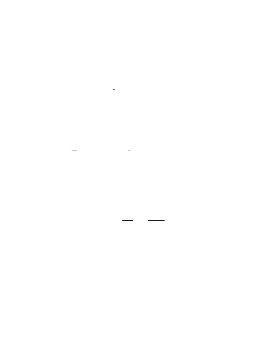
(
)
q ,t
f
f
(
)
q ,t
i
i
t = t
1
q
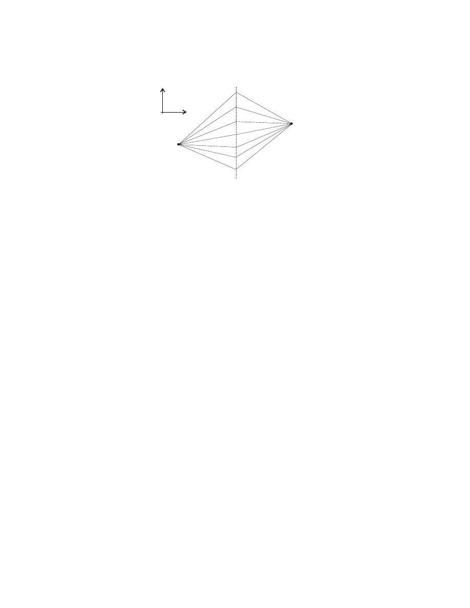
t
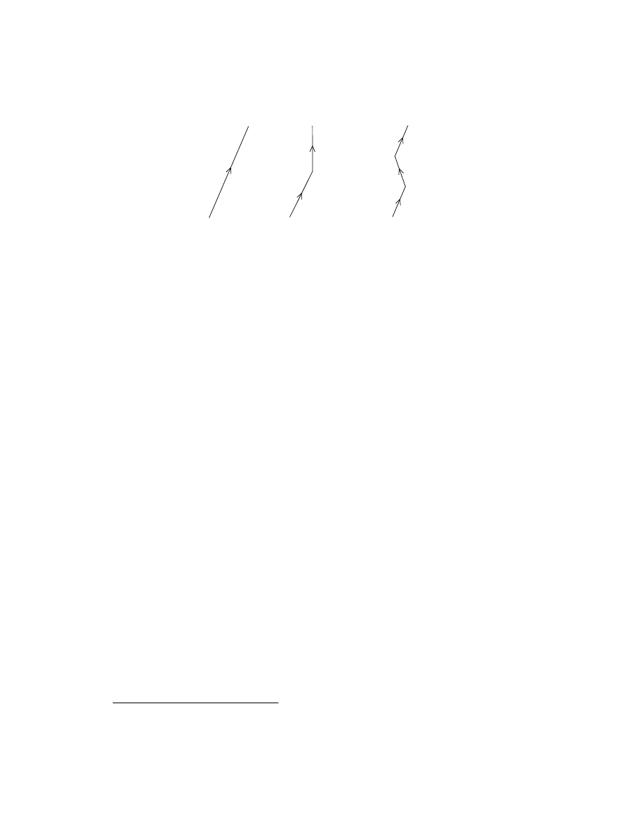
Figure 1: The various two-legged paths that are considered in the calculation of
hq
f
, t
f
|q
i
, t
i
i
Multiplying by e
iHt
0
on the left and e
−iHt
0
on the right yields that
1 =
Z
dq
0
|q
0
, t
0
ihq
0
, t
0
|.
(7)
Now, using the completeness of the |q, ti basis, we may write
ψ(q
f
, t
f
) =
Z
dq
i
hq
f
, t
f
|q
i
, t
i
ihq
i
, t
i
|ψi
=
Z
dq
i
hq
f
, t
f
|q
i
, t
i
iψ(q
i
, t
i
).
(8)
The quantity hq
f
, t
f
|q
i
, t
i
i is called the propagator and it represents the probability
amplitudes (expansion coefficients) associated with the decomposition of ψ(q
f
, t
f
)
in terms of ψ(q
i
, t
i
). If ψ(q
i
, t
i
) has the form of a spatial delta function δ(q
0
), then
ψ(q
f
, t
f
) = hq
f
, t
f
|q
0
, t
i
i. That is, if we know that the particle is at q
0
at some time
t
i
, then the probability that it will be later found at a position q
f
at a time t
f
is
P (q
f
, t
f
; q
0
, t
i
) = |hq
f
, t
f
|q
i
, t
0
i|
2
.
(9)
It is for this reason that we sometimes call the propagator a correlation function.
Now, using completeness, it is easily seen that the propagator obeys a composi-
tion equation:
hq
f
, t
f
|q
i
, t
i
i =
Z
dq
1
hq
f
, t
f
|q
1
, t
1
ihq
1
, t
1
|q
i
, t
i
i.
(10)
This can be understood by saying that the probability amplitude that the position
of the particle is q
i
at time t
i
and q
f
at time t
f
is equal to the sum over q
1
of the
probability that the particle traveled from q
i
to q
1
(at time t
1
) and then on to q
f
.
In other words, the probability amplitude that a particle initially at q
i
will later
be seen at q
f
is the sum of the probability amplitudes associated with all possible
3
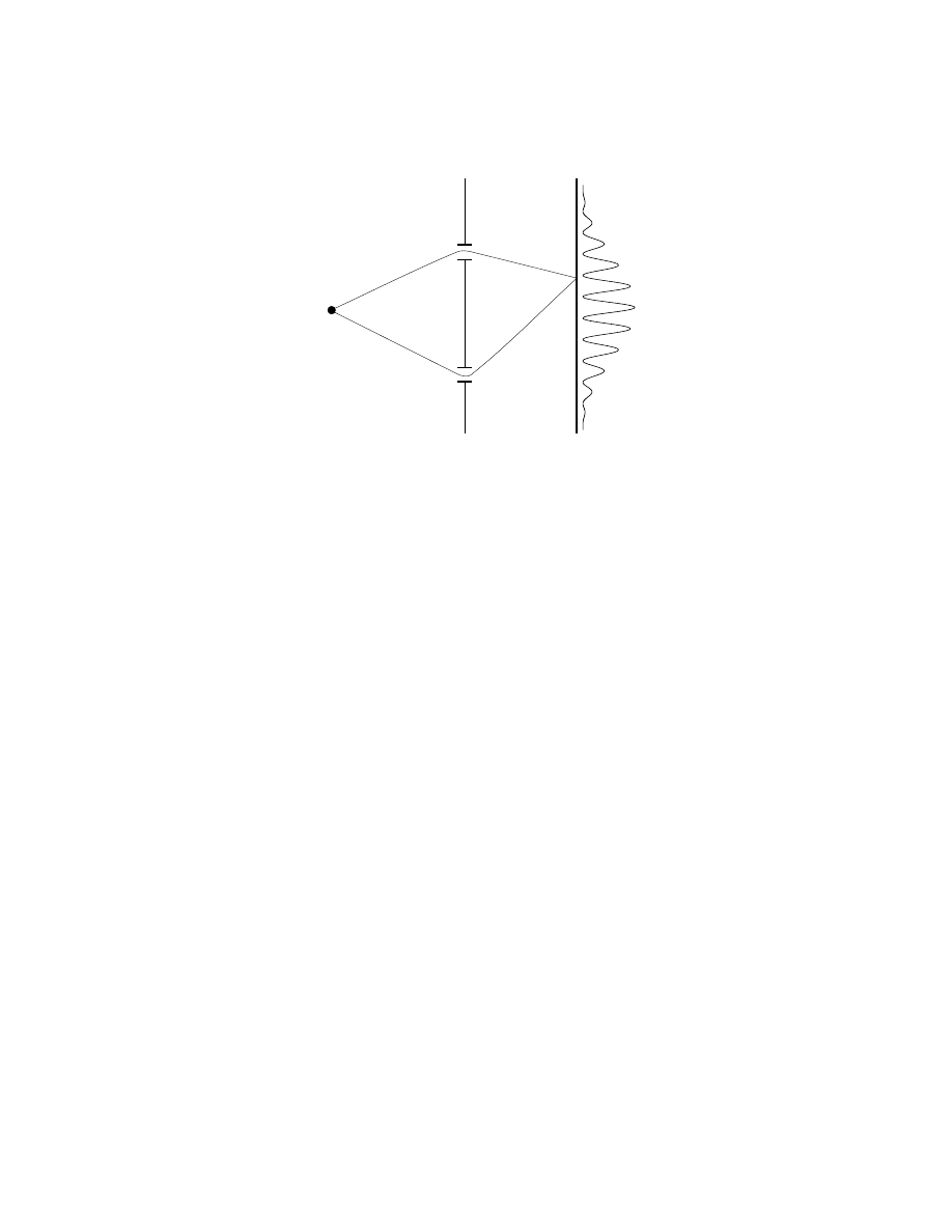
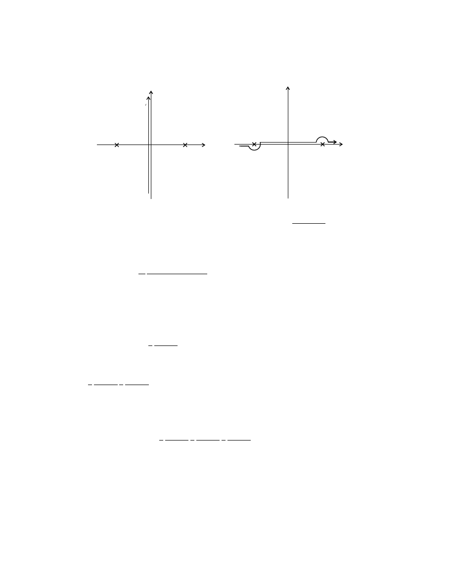
1
2
A
B
Figure 2: The famous double-slit experiment
two-legged paths between q
i
and q
f
, as seen in figure 1. This is the meaning of
the oft-quoted phrase: “motion in quantum mechanics is considered to be a sum
over paths”. A particularly neat application comes from the double slit experiment
that introductory texts use to demonstrate the wave nature of elementary particles.
The situation is sketched in figure 2. We label the initial point (q
i
, t
i
) as 1 and the
final point (q
f
, t
f
) as 2. The amplitude that the particle (say, an electron) will be
found at 2 is the sum of the amplitude of the particle traveling from 1 to A and
then to 2 and the amplitude of the particle traveling from 1 to B and then to 2.
Mathematically, we say that
h2|1i = h2|AihA|1i + h2|BihB|1i.
(11)
The presence of the double-slit ensures that the integral in (10) reduces to the two-
part sum in (11). When the probability |h2|1i|
2
is calculated, interference between
the h2|AihA|1i and h2|BihB|1i terms will create the classic intensity pattern on the
screen.
There is no reason to stop at two-legged paths. We can just as easily separate
the time between t
i
and t
f
into n equal segments of duration τ = (t
f
− t
i
)/n. It
then makes sense to relabel t
0
= t
i
and t
n
= t
f
. The propagator can be written as
hq
n
, t
n
|q
0
, t
0
i =
Z
dq
1
· · · dq
n−1
hq
n
, t
n
|q
n−1
, t
n−1
i · · · hq
1
, t
1
|q
0
, t
0
i.
(12)
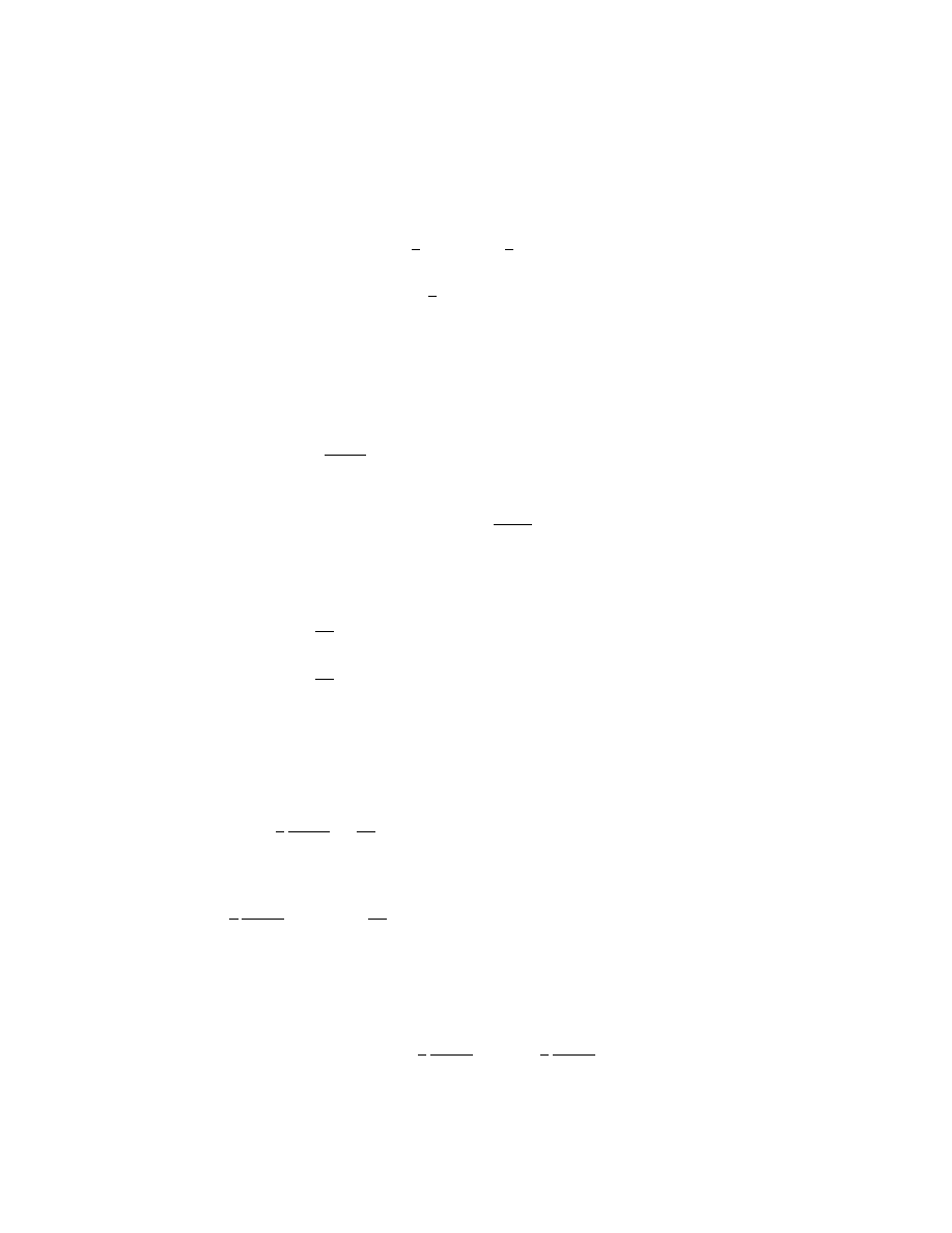
We take the limit n → ∞ to obtain an expression for the propagator as a sum over
infinite-legged paths, as seen in figure 3. We can calculate the propagator for small
time intervals τ = t
j+1
− t
j
for some j between 1 and n − 1. We have
hq
j+1
, t
j+1
|q
j
, t
j
i = hq
j+1
|e
−iHt
j+1
e
+iHt
j
|q
j
i
4
t
0
t
1
t
2
t
3
t
4
t
5
q
i
q
f
q
i
q
f
n
OO
Figure 3: The continuous limit of a collection of paths with a finite number of legs
= hq
j+1
|(1 − iHτ + O(τ
2
)|q
j
i
= δ(q
j+1
− q
j
) − iτ hq
j+1
|H|q
j
i
=
1
2π
Z
dp e
ip(q
j+1
−q
j
)
−
iτ
2m
hq
j+1
|p
2
|q
j
i
−iτ hq
j+1
|V (q)|q
j
i,
(13)
where we have assumed a Hamiltonian of the form
H(p, q) =
p
2
2m
+ V (q).
(14)
Now,
hq
j+1
|p
2
|q
j
i =
Z
dp dp
0
hq
j+1
|p
0
ihp
0
|p
2
|pihp|q
j
i,
(15)
where |pi is an eigenstate of momentum such that
p|pi = |pip,
hq|pi =
1
√
2π
e
ipq
,
hp|p
0
i = δ(p − p
0
).
(16)
Putting these expressions into (15) we get
hq
j+1
|p
2
|q
j
i =
1
2π
Z
dp p
2
e
ip(q
j+1
−q
j
)
,
(17)
where we should point out that p
2
is a number, not an operator. Working on the
other matrix element in (13), we get
hq
j+1
|V (q)|q
j
i = hq
j+1
|q
j
iV (q
j
)
= δ(q
j+1
− q
j
)V (q
j
)
=
1
2π
Z
dp e
ip(q
j+1
−q
j
)
V (q
j
).
5

Putting it all together
hq
j+1
, t
j+1
|q
j
, t
j
i =
1
2π
Z
dp e
ip(q
j+1
−q
j
)
£
1 − iτ H(p, q
j
) + O(τ
2
)
¤
=
1
2π
Z
dp exp
·
iτ
µ
p
∆q
j
τ
− H(p, q
j
)
¶¸
,
where ∆q
j
≡ q
j+1
− q
j
. Substituting this expression into (12) we get
hq
n
, t
n
|q
0
, t
0
i =
Z
dp
0
n−1
Y
i=1
dq
i
dp
i
2π
exp
i
n−1
X
j=0
τ
µ
p
j
∆q
j
τ
− H(p
j
, q
j
)
.
(18)
In the limit n → ∞, τ → 0, we have
n−1
X
j=0
τ →
Z
t
n
t
0
dt,
∆q
j
τ
→
dq
dt
= ˙q,
dp
0
n
Y
i=1
dq
i
dp
i
2π
→ [dq] [dp],
(19)
and
hq
n
, t
n
|q
0
, t
0
i =
Z
[dq] [dp] exp
½
i
Z
t
n
t
0
dt [p ˙q − H(p, q)]
¾
.
(20)
The notation [dq] [dp] is used to remind us that we are integrating over all possible
paths q(t) and p(t) that connect the points (q
0
, t
0
) and (q
n
, t
n
). Hence, we have
succeed in writing the propagator hq
n
, t
n
|q
0
, t
0
i as a functional integral over the
all the phase space trajectories that the particle can take to get from the initial
to the final points. It is at this point that we fully expect the reader to scratch
their heads and ask: what exactly is a functional integral? The simple answer is a
quantity that arises as a result of the limiting process we have already described.
The more complicated answer is that functional integrals are beasts of a rather
vague mathematical nature, and the arguments as to their standing as well-behaved
entities are rather nebulous. The philosophy adopted here is in the spirit of many
mathematically controversial manipulations found in theoretical physics: we assume
that everything works out alright.
The argument of the exponential in (20) ought to look familiar. We can bring
this out by noting that
1
2π
Z
dp
i
e
iτ
h
p
i
∆qi
τ
−H(p
i
,q
i
)
i
=
1
2π
exp
(
iτ
"
m
2
µ
∆q
i
τ
2
− V (q
i
)
#)
×
Z
dp
i
exp
"
−
iτ
2m
µ
p −
m∆q
i
τ
2
#
=
³ m
2πiτ
´
1/2
exp
(
iτ
"
m
2
µ
∆q
i
τ
2
− V (q
i
)
#)
.
6
Using this result in (18) we obtain
hq
n
, t
n
|q
0
, t
0
i =
³ m
2πiτ
´
n/2
Z
n−1
Y
i=1
dq
i
exp
i
n−1
X
j=0
τ
"
m
2
µ
∆q
j
τ
2
− V (q
j
)
#
→ N
Z
[dq] exp
·
i
Z
t
n
t
0
dt
µ
1
2
m ˙q
2
− V (q)
¶¸
,
(21)
where the limit is taken, as usual, for n → ∞ and τ → 0. Here, N is an infinite
constant given by
N = lim
n→∞
³ m
2πiτ
´
n/2
.
(22)
We won’t worry too much about the fact that N diverges because we will later
normalize our transition amplitudes to be finite. Recognizing the Lagrangian L =
T − V in equation (21), we have
hq
n
, t
n
|q
0
, t
0
i = N
Z
[dq] exp
·
i
Z
t
n
t
0
L(q, ˙q) dt
¸
= N
Z
[dq] e
iS[q]
,
(23)
where S is the classical action, given as a functional of the trajectory q = q(t).
Hence, we see that the propagator is the sum over paths of the amplitude e
iS[q]
,
which is the amplitude that the particle follows a given trajectory q(t). Historically,
Feynman demonstrated that the Schr¨odinger equation could be derived from equa-
tion (23) and tended to regard the relation as the fundamental quantity in quantum
mechanics. However, we have assumed in our derivation that the potential is a
function of q and not p. If we do indeed have velocity-dependent potentials, (23)
fails to recover the Schr¨odinger equation. We will not go into the details of how to
fix the expression here, we will rather heuristically adopt the generalization of (23)
for our later work in with quantum fields
3
.
An interesting consequence of (23) is seen when we restore ~. Then
hq
n
, t
n
|q
0
, t
0
i = N
Z
[dq] e
iS[q]/
~
.
(24)
The classical limit is obtained by taking ~ → 0. Now, consider some trajectory q
0
(t)
and neighbouring trajectory q
0
(t)+δq(t), as shown in figure 4. The action evaluated
along q
0
is S
0
while the action along q
0
+δq is S
0
+δS. The two paths will then make
contributions exp(iS
0
/~) and exp[i(S
0
+ δS)/~] to the propagator. For ~ → 0, the
phases of the exponentials will become completely disjoint and the contributions
will in general destructively interfere. That is, unless δS = 0 in which case all
neighbouring paths will constructively interfere. Therefore, in the classical limit
the propagator will be non-zero for points that may be connected by a trajectory
3
The generalization of velocity-dependent potentials to field theory involves the quantization of
non-Abelian gauge fields
7

q t
( )
q t
q t
( ) +
( )
d
q
q
i
f
Figure 4: Neighbouring particle trajectories. If the action evaluated along q(t) is
stationary (i.e. δS = 0), then the contribution of q(t) and it’s neighbouring paths
q(t) + δq(t) to the propagator will constructively interfere and reconstruct the clas-
sical trajectory in the limit ~ → 0
.
satisfying δS[q]|
q=q
0
; i.e. for paths connected by classical trajectories determined by
Newton’s 2
nd
law. We have hence seen how the classical principle of least action
can be understood in terms of the path integral formulation of quantum mechanics
and a corresponding principle of stationary phase.
3
Perturbation theory, the scattering matrix
and Feynman rules
In practical calculations, it is often impossible to solve the Schr¨odinger equation
exactly. In a similar manner, it is often impossible to write down analytic expressions
for the propagator hq
f
, t
f
|q
i
, t
i
i for general potentials V (q). However, if one assumes
that the potential is small and that the particle is nearly free, one makes good
headway by using perturbation theory. We follow section 5.2 in Ryder [1].
In this section, we will go over from the general configuration coordinate q to
the more familiar x, which is just the position of the particle in a one-dimensional
space. The extension to higher dimensions, while not exactly trivial, is not difficult
to do. We assume that the potential that appears in (23) is “small”, so we may
perform an expansion
exp
·
−i
Z
t
n
t
0
V (x, t) dt
¸
= 1 − i
Z
t
n
t
0
V (x, t) dt −
1
2!
·Z
t
n
t
0
V (x, t) dt
¸
2
+ · · · .
(25)
We adopt the notation that K = K(x
n
, t
n
; x
0
, t
0
) = hx
n
, t
n
|x
0
, t
0
i. Inserting the
expansion (25) into the propagator, we see that K possesses and expansion of the
form:
K = K
0
+ K
1
+ K
2
+ · · ·
(26)
8

The K
0
term is
K
0
= N
Z
[dx] exp
·
i
Z
1
2
m ˙x
2
dt
¸
.
(27)
If we turned off the potential, the full propagator would reduce to K
0
. It is for this
reason that we call K
0
the free particle propagator, it represents the amplitude that
a free particle known to be at x
0
at time t
0
will later be found at x
n
at time t
n
.
Going back to the discrete expression:
K
0
= lim
n→∞
³ m
2πiτ
´
n/2
Z
n−1
Y
i=1
dx
i
exp
imτ
2
n−1
X
j=0
(x
j+1
− x
j
)
2
.
(28)
This is a doable integral because the argument of the exponential is a simple
quadratic form. We can hence diagonalize it by choosing an appropriate rotation of
the x
j
Cartesian variables of integration. Conversely, we can start calculating for
n = 2 and solve the general n case using induction. The result is
K
0
= lim
n→∞
³ m
2πiτ
´
n/2
1
n
1/2
µ
2πiτ
m
(n−1)/2
exp
·
im(x
n
− x
0
)
2
2nτ
¸
.
(29)
Now, (t
n
− t
0
)/n = τ , so we finally have
K
0
(x
n
− x
0
, t
n
− t
0
) =
·
m
2πi(t
n
− t
0
)
¸
1/2
exp
·
im(x
n
− x
0
)
2
2(t
n
− t
0
)
¸
,
t
n
> t
0
.
(30)
Here, we’ve noted that the substitution nτ = (t
n
− t
0
) is only valid for t
n
> t
0
. In
fact, if K
0
is non-zero for t
n
> t
0
it must be zero for t
0
> t
n
. To see this, we note
that the calculation of K
0
involved integrations of the form:
Z
∞
−∞
e
iαx
2
dx =
1
2
Z
∞
0
e
iαx
2
dx
=
i
−1/2
4
Z
i∞
0
e
αs
s
1/2
ds
=
i
−1/2
4
Z
i∞
−i∞
Θ(−is)
e
αs
s
1/2
ds,
where α ∝ sign(τ ) = sign(t
n
− t
0
). Now, we can either choose the branch of s
−1/2
to be in either the left- or righthand part of the complex s-plane. But, we need
to complete the contour in the lefthand plane if α > 0 and the righthand plane if
α < 0. Hence, the integral can only be non-zero for one case of the sign of α. The
choice we have implicitly made is the the integral is non-zero for α ∝ (t
n
− t
0
) > 0,
hence it must vanish for t
n
< t
0
. When we look at equation (8) we see that K
0
is little more than a type of kernel for the integral solution of the free-particle
Schr¨odinger equation, which is really a statement about Huygen’s principle. Our
9

choice of K
0
obeys causality in that the configuration of the field at prior times
determines the form of the field in the present. We have hence found a retarded
propagator. The other choice for the boundary conditions obeyed by K
0
yields
the advanced propagator and a version of Huygen’s principle where future field
configurations determine the present state. The moral of the story is that, if we
choose a propagator that obeys casuality, we are justified in writing
K
0
(x, t) = Θ(t)
h m
2πit
i
1/2
exp
·
imx
2
2t
¸
.
(31)
Now, we turn to the calculation of K
1
:
K
1
= −iN
Z
[dx] exp
·
i
Z
1
2
m ˙x
2
dt
¸ Z
dt V (x(t), t).
(32)
Moving again to the discrete case:
K
1
= −iβ
n/2
Z
dx
1
· · · dx
n−1
exp
imτ
2
n−1
X
j=0
(x
j+1
− x
j
)
2
n−1
X
i=1
τ V (x
i
, t
i
),
(33)
where β = m/2πiτ and the limit n → ∞ is understood. Let’s take the sum over i
(which has replaced the integral over t) in front of the spatial integrals. Also, let’s
split up the sum over j in the exponential to a sum running from 0 to i − 1 and a
sum running from i to n − 1. Then
K
1
= −i
n−1
X
i=1
τ
Z
dx
i
β
i/2
Z
dx
1
· · · dx
i−1
exp
imτ
2
i−1
X
j=0
(x
j+1
− x
j
)
2
V (x
i
, t
i
)
×β
(n−i)/2
Z
dx
i+1
· · · dx
n−1
exp
imτ
2
n−1
X
j=i
(x
j+1
− x
j
)
2
.
(34)
We recognize two factors of the free-particle propagator in this expression, which
allows us to write
K
1
= −i
n−1
X
i=1
τ
Z
dx K
0
(x − x
0
, t
i
− t
0
)V (x, t
i
)K
0
(x
n
− x, t
n
− t
i
).
(35)
Now, we can replace
P
n−1
i=1
τ by
R
t
n
t
0
dt and t
i
→ t in the limit n → ∞. Since
K
0
(x − x
0
, t − t
0
) = 0 for t < t
0
and K
0
(x
n
− x, t
n
− t) for t > t
n
, we can extend the
limits on the time integration to ±∞. Hence,
K
1
= −i
Z
dx dt K
0
(x
n
− x, t
n
− t)V (x, t)K
0
(x − x
0
, t − t
0
).
(36)
10

In a similar fashion, we can derive the expression for K
2
:
K
2
=
(−i)
2
2!
β
n/2
Z
dx
1
· · · dx
n−1
exp
imτ
2
n−1
X
j=0
(x
j+1
− x
j
)
2
(37)
×
n−1
X
i=1
τ V (x
i
, t
i
)
n−1
X
k=1
τ V (x
k
, t
k
).
(38)
We would like to play the same trick that we did before by splitting the sum over
j into three parts with the potential terms sandwiched in between. We need to
construct the middle j sum to go from an early time to a late time in order to replace
it with a free-particle propagator. But the problem is, we don’t know whether t
i
comes before or after t
k
. To remedy this, we split the sum over k into a sum from
1 to i − 1 and then a sum from i to n − 1. In each of those sums, we can easily
determine which comes first: t
i
or t
k
. Going back to the continuum limit:
K
2
=
(−i)
2
2!
Z
dx
1
dx
2
Z
t
n
t
0
dt
1
·Z
t
1
t
0
dt
2
K
0
(x
n
− x
1
, t
n
− t
1
)
×V (x
1
, t
1
)K
0
(x
1
− x
2
, t
1
− t
2
)V (x
2
, t
2
)K
0
(x
2
− x
0
, t
2
− t
0
)
+
Z
t
n
t
1
dt
2
K
0
(x
n
− x
2
, t
n
− t
2
)V (x
2
, t
2
)K
0
(x
2
− x
1
, t
2
− t
1
)
×V (x
1
, t
1
)K
0
(x
1
− x
0
, t
1
− t
0
)
¸
(39)
But, we can extend the limits on the t
2
integration to t
0
→ t
n
by noting the middle
propagator is zero for t
2
> t
1
. Similarly, the t
2
limits on the second integral can
be extended by observing the middle propagator vanishes for t
1
> t
2
. Hence, both
integrals are the same, which cancels the 1/2! factor. Using similar arguments, the
limits of both of the remaining time integrals can be extended to ±∞ yielding our
final result:
K
2
= (−i)
2
Z
dx
1
dx
2
dt
1
dt
2
K
0
(x
n
− x
2
, t
n
− t
2
)V (x
2
, t
2
)
×K
0
(x
2
− x
1
, t
2
− t
1
)V (x
1
, t
1
)K
0
(x
1
− x
0
, t
1
− t
0
).
(40)
Higher order contributions to the propagator follow in a similar fashion. The general
j
th
order correction to the free propagator is
K
j
= (−i)
j
Z
dx
1
. . . dx
j
dt
1
. . . dt
j
K
0
(x
n
− x
j
, t
n
− t
j
)
×V (x
j
) · · · V (x
1
)K
0
(x
1
− x
0
, t
1
− t
0
).
(41)
We would like to apply this formalism to scattering problems where we assume
that the particle is initially in a plane wave state incident on some localized potential.
11

As t → ±∞, we assume the potential goes to zero, which models the fact that the
particle is far away from the scattering region in the distant past and the distant
future. We go over from one to three dimensions and write
ψ(x
f
, t
f
) =
Z
dx
i
K
0
(x
f
− x
i
, t
f
− t
i
)ψ(x
i
, t
i
)
−i
Z
dx
i
dx dt K
0
(x
f
− x, t
f
− t)
×V (x, t)K
0
(x − x
i
, t − t
i
)ψ(x
i
, t
i
) + · · ·
(42)
We push t
i
into the distant past, where the effects of the potential may be ignored,
and take the particle to be in a plane wave state:
ψ
in
(x
i
, t
i
) =
1
√
V
e
−ip
i
·x
i
,
(43)
where we have used a box normalization with V being the volume of the box and
p
i
· x = E
i
t
i
− p
i
· x
i
. The “in” label on the wavefunction is meant to emphasize that
it is the form of ψ before the particle moves into the scattering region. We want to
calculate the first integral in (42) using the 3D generalization of (31):
K
0
(x, t) = −iΘ(t)
µ
λ
π
3/2
e
λx
2
,
(44)
where λ = im/2t. Hence,
Z
dx
i
K
0
(x
f
− x
i
, t
f
− t
i
)ψ
in
(x
i
, t
i
) = −
i
√
V
µ
λ
π
3/2
×e
−iE
i
t
i
Z
dx
i
e
λ(x
f
−x
i
)
2
+ip
i
·x
i
.
(45)
This integral reduces to ψ
in
(x
f
, t
f
) as should have been expected, because K
0
is the
free particle propagator and must therefore propagate plane waves into the future
without altering their form. We also push t
f
into the infinite future where the effects
of the potential can be ignored. Then,
ψ
+
(x
f
, t
f
) = ψ
in
(x
f
, t
f
) − i
Z
dx
i
dx dt K
0
(x
f
− x, t
f
− t)
×V (x, t)K
0
(x − x
i
, t − t
i
)ψ
in
(x
i
, t
i
) + · · ·
(46)
The “+” notation on ψ is there to remind us that ψ
+
is the form of the wave function
after it interacts with the potential. What we really want to do is Fourier analyze
ψ
+
(x
f
, t
f
) into momentum eigenstates to determine the probability amplitude for
a particle of momentum p
i
becoming a particle of momentum p
f
after interacting
12

with the potential. Defining ψ
out
(x
f
, t
f
) as a state of momentum p
f
in the distant
future:
ψ
out
(x
f
, t
f
) =
1
√
V
e
−ip
f
·x
f
,
(47)
we can write the amplitude for a transition from p
i
to p
f
as
S
f i
= hψ
out
|ψ
+
i.
(48)
Inserting the unit operator 1 =
R
dx
f
|x
f
, t
f
ihx
f
, t
f
| into (48) and using the propa-
gator expansion (46), we obtain
S
f i
= δ(p
f
− p
i
) − i
Z
dx
i
dx
f
dx dt ψ
∗
out
(x
f
, t
f
)K
0
(x
f
− x, t
f
− t)
×V (x, t)K
0
(x − x
i
, t − t
i
)ψ
in
(x
i
, t
i
) + · · ·
(49)
The amplitude S
f i
is the f i component of what is known as the S or scattering
matrix. This object plays a central rˆole in scattering theory because it answers all
the questions that one can experimentally ask about a physical scattering process.
What we have done is expand these matrix elements in terms of powers of the
scattering potential. Our expansion can be given in terms of Feynman diagrams
according to the rules:
1. The vertex of this theory is attached to two legs and a spacetime point (x, t).
2. Each vertex comes with a factor of −iV (x, t).
3. The arrows on the lines between vertices point from the past to the future.
4. Each line going from (x, t) to (x
0
, t
0
) comes with a propagator K
0
(x
0
−x, t
0
−t).
5. The past external point comes with the wavefunction ψ
in
(x
i
, t
i
), the future
one comes with ψ
∗
out
(x
f
, t
f
).
6. All spatial coordinates and internal times are integrated over.
Using these rules, the S matrix element may be represented pictorially as in figure 5.
We note that these rules are for configuration space only, but we could take Fourier
transforms of all the relevant quantities to get momentum space rules. Obviously,
the Feynman rules for the Schr¨odinger equation do not result in a significant sim-
plification over the raw expression (49), but it is important to notice how they were
derived: using simple and elegant path integral methods.
13
x , t
i
i
x , t
f
f
x , t
i
i
x , t
f
f
x , t
1
1
x , t
2
2
x , t
i
i
x , t
f
f
x , t
1
1
S
fi
=
+
+
+
…
Figure 5: The expansion of S
f i
in terms of Feynman diagrams
4
Sources, vacuum-to-vacuum transitions and
time-ordered products
We now consider a alteration of the system Lagrangian that models the presence
of a time-dependent “source”. Our discussion follows section 5.5 of Ryder [1] and
chapters 1 and 2 of Brown [3]. In this context, we call any external agent that
may cause a non-relativistic system to make a transition from one energy eigenstate
to another a “source”. For example, a time-dependent electric field may induce a
charged particle in a one dimensional harmonic oscillator potential to go from one
eigenenergy to another. In the context of field theory, a time-dependent source may
result in spontaneous particle creation
4
. In either case, the source can be modeled
by altering the Lagrangian such that
L(q, ˙q) → L(q, ˙q) + J(t)q(t).
(50)
The source J(t) will be assumed to be non-zero in a finite interval t ∈ [t
1
, t
2
]. We
take T
2
> t
2
and T
1
< t
1
. Given that the particle was in it’s ground state at
T
1
→ −∞, what is the amplitude that the particle will still be in the ground state
at time T
2
→ ∞?
To answer that question, consider
hQ
2
, T
2
|Q
1
, T
1
i
J
=
Z
dq
1
dq
2
hQ
2
, T
2
|q
2
, t
2
ihq
2
, t
2
|q
1
, t
1
i
J
hq
1
, t
1
|Q
1
, T
1
i
=
Z
dq
1
dq
2
hQ
2
|e
−iHT
2
e
iHt
2
|q
2
ihq
2
, t
2
|q
1
, t
1
i
J
×hq
1
|e
−iHt
1
e
iHT
1
|Q
1
i
=
X
mn
Z
dq
1
dq
2
hQ
2
|e
−iHT
2
|mihm|e
iHt
2
|q
2
ihq
2
, t
2
|q
1
, t
1
i
J
×hq
1
|e
−iHT
1
|nihn|e
iHt
1
|Q
1
i
4
cf. PHYS 703 March 14, 2000 lecture
14
T
Te
-id
-d
-d
J = 0
J = 0
J = 0
t
2
t
1
Figure 6: The rotation of the time axis needed to isolate the ground state contribu-
tion to the propagator
=
X
mn
e
−i(E
n
T
2
−E
m
T
1
)
φ
m
(Q
2
)φ
∗
n
(Q
1
)
×
Z
dq
1
dq
2
φ
∗
m
(q
2
, t
2
)hq
2
, t
2
|q
1
, t
1
i
J
φ
n
(q
1
, t
1
),
where we have introduced a basis of energy eigenstates H|ni = E
n
|ni and energy
eigenfunctions φ
n
(q, t) = e
−iE
n
t
hq|mi with φ
n
(q) = hq|ni. The J subscripts on the
propagators remind us that the source is to be accounted for. It is important to
note that φ
n
(q) is only a true eigenfunction for times when the source is not acting;
i.e. prior to t
1
and later than t
2
. The integral on the last line can be thought of
as a wavefunction, φ
n
(q
1
, t
1
), that is propagated through the time when the source
is acting by hq
2
, t
2
|q
1
, t
1
i
J
, and is then dotted with a wavefunction φ
∗
m
(q
2
, t
2
). But,
φ
n
(q
1
, t
1
) and φ
∗
m
(q
2
, t
2
) are energy eigenfunctions for times before and after the
source, respectively. Hence, the integral is the amplitude that an energy eigenstate
|ni will become an energy eigenstate |mi through the action of the source. Now,
let’s perform a rotation of the time-axis in the complex plane by some small angle
−δ (δ > 0), as shown in figure 6. Under such a transformation
T
1
→ T
1
+ i|T
1
|δ
(51)
T
2
→ T
2
− i|T
2
|δ,
(52)
where we have chosen the axis of rotation to lie between T
1
and T
2
. We see
that the exponential term e
−i(E
n
T
2
−E
m
T
1
)
will acquire a damping that goes like
e
−δ(E
n
|T
2
|+E
m
|T
1
|)
. As we push T
1
→ −∞ and T
2
→ ∞, the damping will become
infinite for each term in the sum, except for the ground state which we can set to
have an energy of E
0
≥ 0. Therefore,
lim
T →∞ e
−iδ
hQ
2
, T |Q
1
, −T i
J
= e
−iE
0
(T
2
−T
1
)
φ
0
(Q
2
)φ
∗
0
(Q
1
)
(53)
×
Z
dq
1
dq
2
φ
∗
0
(q
2
, t
2
)hq
2
, t
2
|q
1
, t
1
i
J
φ
0
(q
1
, t
1
),
δ > 0,
where we have set T
2
= −T
1
= T for convenience. Now, if we take t
2
and t
1
to ±∞
respectively, the integral reduces to the amplitude that a wavefunction which has
15
the form of φ
0
(q) in the distant past will still have the form of φ
0
(q) in the distant
future. In other words, it is the ground-to-ground state transition amplitude, which
we denote by
h0, ∞|0, −∞i
J
∝
lim
T →∞ e
−iδ
hQ
2
, T |Q
1
, −T i
J
,
(54)
where the constant of proportionality depends on Q
1
, Q
2
and T . Now, instead
of rotating the contour of the the time-integration, we could have added a small
term −i²q
2
/2 to the Hamiltonian. Using first order perturbation theory, this shifts
the energy levels by an amount δE
n
= −i²hn|q
2
|ni/2. For most problems (i.e. the
harmonic oscillator, hydrogen atom), the expectation value of q
2
increases with
increasing energy. Assuming that this is the case for the problem we are doing, we
see that the first order shift in the eigenenergy accomplishes the same thing as the
rotation of the time axis in (54). But, subtracting i²q
2
/2 from H is the same thing
as adding i²q
2
/2 from L
5
. Therefore,
h0, ∞|0, −∞i
J
∝
Z
[dQ] exp
½
i
Z
∞
−∞
dt
·
L(Q, ˙
Q) + JQ +
1
2
i²q
2
¸¾
.
(55)
Finally, want to normalize this result such that if the source is turned off, the
amplitude h0, ∞|0, −∞i is unity. Defining
Z[J] =
R
[dQ] exp
n
i
R
∞
−∞
dt
h
L(Q, ˙
Q) + JQ +
1
2
i²Q
2
io
R
[dQ] exp
n
i
R
∞
−∞
dt
h
L(Q, ˙
Q) +
1
2
i²Q
2
io
,
(56)
we have
h0, ∞|0, −∞i
J
= Z[J].
(57)
Before moving on the the next section, we would like to establish a result that will
prove very useful later when we consider field theories. We first define the functional
derivative of Z[J] with respect to J(t
0
). Essentially, the functional derivative of a
functional f [y], where y = y(x), is the derivative of the discrete expression with
respect to the value of y at a given x. For example, the discrete version of Z[J] is
Z (τ J(t
0
), τ J(t
1
) . . . τ J(t
n−1
)) ∝
Z
exp
iτ
n−1
X
j=0
h
L(Q
j
, ˙
Q
j
)
+ J(t
j
)Q
j
+
1
2
i²Q
2
j
¸)
n−1
Y
i=1
dQ
i
,
(58)
where we have indicated that the discrete version of Z[J] is an ordinary function of n
variables τ J(t
j
) and omitted the normalization factor. We have explicitly included
5
An alternative procedure for singling out the ground state contribution comes from considering
t to be purely imaginary, i.e. consideration of Euclidean space. This is discussed in the next section.
16
the weighting factor τ with each of the discrete variables to account for the fact
that as n → ∞, each J(t
k
) covers a smaller and smaller portion of the integration
interval. The functional derivative of Z[J] with respect to J(t
k
) is then the partial
derivative of the discrete expression with respect to τ J(t
k
). Going back to the
continuum limit, we write the functional derivative of Z[J] with respect to Q(t
1
) as:
δZ[J]
δJ(t
1
)
∝ i
Z
[dQ]Q(t
1
) exp
½
i
Z
∞
−∞
dt
·
L(Q, ˙
Q) + JQ +
1
2
i²Q
2
¸¾
.
(59)
In a similar fashion, we have
δ
n
Z[J]
δJ(t
1
) · · · δJ(t
n
)
∝ i
n
Z
[dQ]Q(t
1
) · · · Q(t
n
)
× exp
½
i
Z
∞
−∞
dt
·
L(Q, ˙
Q) + JQ +
1
2
i²Q
2
¸¾
.
(60)
We notice a similarity between this expression and the expression from statistical
mechanics that gives the average value of a microscopic variable in the canonical
ensemble. We argue that equation (60) gives the exact same thing: the expectation
value of Q(t
1
) · · · Q(t
n
). There is one wrinkle, however, which we now proceed to
outline. Consider, with t
k
> t
k
0
,
hq
f
, t
f
|q(t
k
)q(t
k
0
)|q
i
, t
i
i =
Z
dq
1
· · · dq
n−1
hq
f
, t
f
|q
n−1
, t
n−1
i · · ·
hq
k
, t
k
|q(t
k
)|q
k−1
, t
k−1
i · · · hq
k
0
, t
k
0
|q(t
k
0
)|q
k
0
−1
, t
k
0
−1
i
· · · hq
1
, t
1
|q
i
, t
i
i
=
Z
dq
1
· · · dq
n−1
q(t
k
)q(t
k
0
)hq
f
, t
f
|q
n−1
, t
n−1
i · · ·
hq
1
, t
1
|q
i
, t
i
i.
(61)
By pushing t
i
→ −∞ e
−iδ
and t
f
→ ∞ e
−iδ
, we can repeat our previous manipula-
tions to show that
Z
dq
1
· · · dq
n−1
q(t
k
)q(t
k
0
)hq
f
, ∞ e
−iδ
|q
n−1
, t
n−1
i · · · hq
1
, t
1
|q
i
, −∞ e
−iδ
i
= N
Z
[dq]q(t
k
)q(t
k
0
) exp
"
i
Z
∞ e
−iδ
−∞ e
−iδ
dt L(Q, ˙
Q)
#
,
(62)
which follows directly from the arguments of section 2, and
hq
f
, ∞ e
−iδ
|q(t
k
)q(t
k
0
)|q
i
, −∞ e
−iδ
i ∝ h0|q(t
k
)q(t
k
0
)|0i,
(63)
which follows from an argument similar to the one we used to calculate the matrix
element h0, ∞|0, −∞i
J
with t
1
= t
k
0
, t
2
= t
k
and J = 0. Just as before, the
17

rotation of the time axis can be achieved by adding i²q
2
/2 to the Lagrangian. This
calculation cannot be repeated for the case t
k
> t
k
0
because the order of q(t
k
)q(t
k
0
)
in hq
f
, t
f
|q(t
k
)q(t
k
0
)|q
i
, t
i
i cannot be switched without introducing terms involving
the commutator of H and q. But, in order to perform the decomposition (61), we
need the late q operator appearing to the left of the earlier q operator. What this
means is that we must be considering the time-ordered product of q(t
k
) and q(t
k
0
).
Putting all of this together along with the expression for the functional derivatives
of Z[J], we get
δ
2
Z[J]
δJ(t
k
)δJ(t
k
0
)
¯
¯
¯
¯
J=0
= i
2
h0|T [q(t
k
)q(t
k
0
)]|0i.
(64)
This is easily generalized to the time order product of many q operators:
δ
n
Z[J]
δJ(t
1
) · · · δJ(t
n
)
¯
¯
¯
¯
J=0
= i
n
h0|T [q(t
1
) · · · q(t
n
)]|0i.
(65)
We have demanded strict equality in these expression to ensure that the n = 0 case
returns h0|0i = 1. This is a very important formula for what follows.
5
Free scalar fields
We now move on to the quantum field theory of a scalar field φ(x). In this section
we draw on sections 6.1 and 6.3 of Ryder [1], chapter 2 of Popov [4] and section 3.2
of Brown [3]. The classical field φ is assumed to satisfy the Klein-Gordon equation
(¤ + m
2
)φ = 0.
(66)
We define the vacuum to vacuum transition probability for this theory by
h0, ∞|0, −∞i
J
= Z[J],
(67)
where
Z[J] =
1
Z
0
Z
[dφ] exp
½
i
Z
d
4
x
·
L(φ) + J(x)φ +
1
2
i²φ
2
¸¾
,
(68)
with
Z
0
=
Z
[dφ] exp
½
i
Z
d
4
x
·
L(φ) +
1
2
i²φ
2
¸¾
.
(69)
In this expressions, the measure [dφ] is meant to convey an integration over all field
configurations, which can be achieved in practice by dividing spacetime into N
4
points (t
m
, x
i
, y
j
, z
k
), with m, i, j, k = 1 . . . N . We can schematically merge all of
these indices into a single one n = 1 . . . N
4
. The field is considered to be a collection
of N
4
independent variables, and the functional integration [dφ] becomes
R Q
i
dφ
i
.
The functional Z[J] represents the fundamental object in the theory. Knowledge of
the form of Z[J] allows us to derive all the results that we could hope to obtain from
18

experiments involving the field φ. Such grandiose statements need to be justified,
which we now proceed to do.
We first substitute the Lagrangian appropriate to the Klein-Gordon equation
into the expression for Z[J]:
Z[J] =
1
Z
0
Z
[dφ] exp
µ
i
Z
d
4
x
½
1
2
£
∂
α
φ∂
α
φ − (m
2
− i²)φ
2
¤
+ φJ
¾
.
(70)
Integrating the ∂
α
φ∂
α
φ term by parts and using Gauss’ theorem to discard the
boundary term (assuming φ → 0 at infinity) gives
Z[J] =
1
Z
0
Z
[dφ] exp
µ
−i
Z
d
4
x
½
1
2
φ(¤ + m
2
− i²)φ − φJ
¾
.
(71)
Regarding φ as an integration variable, we can change variables according to
φ(x) → φ(x) + φ
0
(x).
(72)
Noting that
Z
d
4
x φ¤φ
0
=
Z
d
4
x φ
0
¤φ
(73)
using Gauss’ theorem and demanding that φ
0
→ 0 at infinity, we obtain
Z[J] =
1
Z
0
Z
[dφ] exp
µ
−i
Z
d
4
x
½
1
2
φ(¤ + m
2
− i²)φ
+φ(¤ + m
2
− i²)φ
0
+
1
2
φ
0
(¤ + m
2
− i²)φ
0
− (φ + φ
0
)J
¾
.
(74)
Let us demand that
(¤ + m
2
− i²)φ
0
= J(x).
(75)
We can solve this equation by introducing the Feynman propagator, which satisfies
(¤ + m
2
− i²)∆
F
(x) = −δ
4
(x).
(76)
Hence,
φ
0
= −
Z
∆
F
(x − y)J(y) d
4
y.
(77)
We then obtain for Z[J]:
Z[J] =
1
Z
0
exp
·
−
i
2
Z
J(x)∆
F
(x − y)J(y) d
4
x d
4
y
¸
×
Z
[dφ] exp
·
−
i
2
Z
φ(¤ + m
2
− i²)φ d
4
x
¸
.
(78)
19
But we know Z[0] = 1, so we must have
Z
0
=
Z
[dφ] exp
·
−
i
2
Z
φ(¤ + m
2
− i²)φ d
4
x
¸
.
(79)
This leads to our final expression:
Z[J] = exp
·
−
i
2
Z
J(x)∆
F
(x − y)J(y) d
4
x d
4
y
¸
.
(80)
Before we move forward, we would like to make a comment on the inclusion of the
i²φ
2
/2 term in our expression for Z[J]. The reader will recall that the reason that we
added this term was to simulate the effects of rotating the time axis by a small angle
−δ in the complex plane. Instead of adding the ²-term, we can instead rotate the
t axis by −π/2 so that t = −iτ . The metric becomes η
αβ
= diag(−1, −1, −1, −1),
which means that we are considering a Euclidean, not Lorentzian, manifold. In that
case, the vacuum-to-vacuum transition amplitude is
Z[J] =
1
Z
0
Z
[dφ] exp
µ
−
Z
dτ dx
½
1
2
£
(∂
τ
φ)
2
+ ∇φ
2
+ m
2
φ
2
¤
− φJ
¾
,
(81)
where ∇ is the del-operator of 3D vector calculus. For J = 0, the argument of
the exponential is negative definite and the integral converges absolutely. So, in
some sense, the rotation of the time axis ensures that the integrals in Z[J] are well
behaved. Another aspect the Euclidean manifold comes from the Euclidean version
of Feynman propagator, which satisfies:
(∂
2
τ
+ ∇
2
− m
2
)∆
F
(x) = δ
4
(x).
(82)
Solving this in Euclidean Fourier space, we get
∆
F
(x) = −
i
(2π)
4
Z
d
4
κ
e
−iκ·x
κ
2
+ m
2
,
(83)
where κ · x = κ
0
τ + k · x and κ
2
= (κ
0
)
2
+ k
2
(the i is there for convenience). If we
change variables according to κ
0
= −ik
0
and τ = it, we get
∆
F
(x) = −
1
(2π)
4
Z
C
0
d
4
k
e
−ik·x
k
2
− m
2
,
(84)
where the k
0
integration is to be performed along the contour C
0
shown in figure
7. But, we can rotate the contour by 90
o
clockwise to C, which is the standard
contour used to calculate the Lorentzian Feynman propagator, defined by (76). To
some extent, this explains why the Feynman propagator has the form that it does:
it is a direct consequence of the need to rotate the time axis to isolate the vacuum
contributions to transition amplitudes and make path integrals converge.
20
=
+w
+w
-w
-w
Re( )
k
0
Re( )
k
0
Im( )
k
0
Im( )
k
0
C
C
Figure 7: Equivalent contours of integration for the calculation of Feynman propa-
gator in the complex k
0
plane. Note the poles at ±ω = ±
p
|k|
2
+ m
2
.
We want to calculate the time-ordered products given by
1
i
n
δ
n
Z[J]
δJ(x
1
) · · · δJ(x
n
)
¯
¯
¯
¯
J=0
= h0|T [φ(x
1
) · · · φ(x
n
)]|0i.
(85)
We recall from the canonical formulation of field theory that h0|T [φ(x)φ(y)]|0i is
the amplitude for the creation of a particle at y and its later destruction at x (or
vice versa, depending on the times associated with x and y). Using (80) and our
previously mentioned notions of functional differentiation, we have
1
i
δ
δJ(x
1
)
Z[J] = −Z[J]
Z
dy ∆
F
(x
1
− y)J(y).
(86)
The second order derivative is
1
i
δ
δJ(x
2
)
1
i
δ
δJ(x
1
)
Z[J] = Z[J]
Z
dy
1
∆
F
(x
1
− y
1
)J(y
1
)
Z
dy
2
∆
F
(x
2
− y
2
)J(y
2
)
+ i∆
F
(x
1
− x
2
)Z[J].
Continuing,
1
i
δ
δJ(x
3
)
1
i
δ
δJ(x
2
)
1
i
δ
δJ(x
1
)
Z[J] =
− i∆
F
(x
1
− x
2
)Z[J]
Z
dy
3
∆
F
(x
3
− y
3
)J(y
3
)
− i∆
F
(x
1
− x
3
)Z[J]
Z
dy
2
∆
F
(x
2
− y
2
)J(y
2
)
− i∆
F
(x
2
− x
3
)Z[J]
Z
dy
1
∆
F
(x
1
− y
1
)J(y
1
)
21

− Z[J]
Z
dy
1
dy
2
dy
3
∆
F
(x
1
− y
1
)J(y
1
)
× ∆
F
(x
2
− y
2
)J(y
2
)∆
F
(x
3
− y
3
)J(y
3
)
Finally, we write down the fourth order derivative:
1
i
δ
δJ(x
4
)
1
i
δ
δJ(x
3
)
1
i
δ
δJ(x
2
)
1
i
δ
δJ(x
1
)
Z[J] = i∆
F
(x
1
− x
2
)i∆
F
(x
3
− x
4
)Z[J]
+ i∆
F
(x
1
− x
3
)i∆
F
(x
2
− x
4
)Z[J]
+ i∆
F
(x
2
− x
3
)i∆
F
(x
1
− x
4
)Z[J]
+ other terms that vanish when J = 0.
When J = 0, these expression give us the following time-ordered products:
h0|T [φ(x
1
)]|0i = 0
(87)
h0|T [φ(x
1
)φ(x
2
)]|0i = i∆
F
(x
1
− x
2
)
(88)
h0|T [φ(x
1
)φ(x
2
)φ(x
3
)]|0i = 0
(89)
h0|T [φ(x
1
)φ(x
2
)φ(x
3
)φ(x
4
)]|0i = i∆
F
(x
1
− x
2
)i∆
F
(x
3
− x
4
)
+ i∆
F
(x
1
− x
3
)i∆
F
(x
2
− x
4
)
+ i∆
F
(x
1
− x
4
)i∆
F
(x
2
− x
3
)
(90)
We call h0|T [φ(x
1
) · · · φ(x
n
)]|0i an n-point correlation function. Generalizing the
pattern above to T products of more field operators, we find that if n is odd, the
n-point function vanishes. On the other hand, if n is even, the correlation func-
tion reduces to the sum all possible permutations of products of 2-point functions
i∆
F
(x − y) with x, y ∈ {x
1
, . . . , x
n
}, x 6= y. When this result is derived from
canonical methods, it is know as Wick’s Theorem.
It is interesting to interpret these results in terms of the Taylor series expansion
of Z[J] about J = 0. To make sense of this object, recall that the Taylor series
expansion of a function of a finite number of variables is
F (y
1
, . . . , y
k
) =
∞
X
n=0
k
X
i
1
=1
· · ·
k
X
i
n
=1
1
n!
y
i
1
. . . y
i
k
∂
n
F
∂y
i
1
. . . ∂y
i
n
¯
¯
¯
¯
y
i
=0
.
(91)
This is expansion is taken about the zero of all of the independent variables. As-
suming the variables are weighted appropriately, when we go to the continuum limit
k → ∞ we obtain that
F [y] =
∞
X
n=0
1
n!
Z
dx
1
· · · dx
n
y(x
1
) · · · y(x
n
)
δ
n
F
δy(x
1
) . . . δy(x
n
)
¯
¯
¯
¯
y=0
.
(92)
Using this expansion, we obtain
22

Z J
[ ] = 1 + x
1
x
2
x
1
x
2
x
3
x
4
+
+
+
+
(
(
x
1
x
2
x
3
x
4
x
1
x
2
x
3
x
4
…
Figure 8: Pictorial representation of the free field generating functional Z[J]
Z[J] = 1 +
i
2
2!
Z
dx
1
dx
2
J(x
1
)J(x
2
)i∆
F
(x
1
− x
2
)
+
i
4
4!
Z
dx
1
dx
2
dx
3
dx
4
J(x
1
)J(x
2
)J(x
3
)J(x
4
)
×
·
i∆
F
(x
1
− x
2
)i∆
F
(x
3
− x
4
) + i∆
F
(x
1
− x
3
)i∆
F
(x
2
− x
4
)
+ i∆
F
(x
1
− x
4
)i∆
F
(x
2
− x
3
)
¸
+ · · ·
(93)
This result is depicted diagrammatically in figure 8. In this figure, we use the
following Feynman rules:
1. Each line is connected to a sink and a source.
2. Each sink or a source is labeled with a spacetime point.
3. A line running between x and y comes with a propagator i∆
F
(x − y).
4. Each source or sink attached to x comes with a factor iJ(x).
5. The collection of all graphs with n sources and sinks is multiplied by 1/n!.
6. All spacetimes coordinates are integrated over.
This first rule ensures that we only include diagrams with an even number of vertices
and that we only consider disconnected graphs. The Feynman diagrams illustrate
the correspondence of Z[J] to the vacuum-to-vacuum transition probability beauti-
fully. Each term in the graph involves the creation of a particle at some point and
its destruction at a later point. The three terms in the 4-vertex graph account for
all possible permutations of particle being created/destroyed at a pair of x
1
, x
2
, x
3
or x
4
. What we would like to do now is move on to the more interesting case of
interacting fields.
6
The generating functional for self-interacting fields
While free field theory has a certain amount of elegance to it, it is not terribly
interesting. In this section, we consider a self-interacting field whose Lagrangian is
23

given by
L(φ) =
1
2
∂
α
φ ∂
α
φ −
1
2
m
2
φ
2
+ L
int
(φ) = L
0
(φ) + L
int
(φ).
(94)
The discussion follows section 6.4 of Ryder [1]. Here, L
int
(φ) is the Lagrangian
describing the self interaction. The generating functional is
Z[J] =
R
[dφ] exp
¡
iS + i
R
d
4
x Jφ
¢
R
[dφ]e
iS
,
(95)
where S is the classical action
S =
Z
d
4
x [L
0
(φ) + L
int
(φ)] = S
0
+ S
int
.
(96)
We have dropped the i²φ
2
/2 term used to single out the ground state, which we can
rationalize by the rotation of the time axis. In this section, we will write the free
field propagator as
Z
0
[J] =
R
[dφ] exp
¡
iS
0
+ i
R
d
4
x Jφ
¢
R
[dφ]e
iS
0
.
(97)
We would like to write Z[J] in a form particularly useful for calculations. We
can’t really reproduce the manipulations of the last section because the L
int
in the
action S introduces difficulties when the shift φ → φ + φ
0
is performed. We will
instead derive a differential equation satisfied by Z[J] and then solve it in terms
of J(x) and the Feynman propagator. The result will be something that we might
have guessed intuitively. What is the equation satisfied by the free field propagator?
Now, we know that
1
i
δ
δJ(x)
Z
0
[J] = −Z
0
[J]
Z
dy ∆
F
(x − y)J(y).
(98)
We operate on both sides with ¤
x
+m
2
and use the defining relation for the Feynman
propagator (76) to get:
(¤
x
+ m
2
)
1
i
δ
δJ(x)
Z
0
[J] = J(x)Z
0
[J].
(99)
The is the differential equation satisfied by Z
0
[J]. In order to find the differential
equation satisfied by Z[J], let us define the functional
ˆ
Z[φ] =
e
iS
R
[dφ] e
iS
.
(100)
Then
Z[J] =
Z
[dφ] ˆ
Z[φ] exp
µ
i
Z
d
4
x Jφ
,
(101)
24
which is the functional equivalent of the Fourier transform. We can functionally
differentiate ˆ
Z[φ] with respect to φ using
S =
Z
d
4
x
·
1
2
∂
α
φ ∂
α
φ −
1
2
m
2
φ
2
+ L
int
(φ)
¸
= −
Z
d
4
x
·
1
2
φ(¤ + m
2
)φ − L
int
¸
,
(102)
where Gauss’ theorem has been used. The superiority of the latter form is that we
can integrate twice by parts to change φ
−
→
¤ φ into φ
←
−
¤ φ. So, when we functionally
differentiate, we can make sure that the φ being acted on by the ¤ operator is
different from the φ being acted on by the δ/δφ. We get
i
δ ˆ
Z[φ]
δφ(x)
= (¤ + m
2
)φ(x) ˆ
Z[φ] − L
0
int
(φ) ˆ
Z[φ],
(103)
where
L
0
int
(φ) =
∂L
int
∂φ
(104)
and ¤ = ¤
x
. We multiply both sides of (103) by exp[i
R
J(y)φ(y) d
4
y] and integrate
over φ, i.e. we take the Fourier transform. The RHS of (103) becomes
RHS =
1
Z
0
(¤ + m
2
)
Z
[dφ]φ(x) exp
·
iS + i
Z
J(y)φ(y) d
4
y
¸
−
1
Z
0
Z
[dφ]L
0
int
(φ) exp
·
iS + i
Z
J(y)φ(y) d
4
y
¸
,
(105)
where we have written
Z
0
=
Z
[dφ]e
iS
.
(106)
Now, it’s easy to see
1
i
δZ[J]
δJ(x)
=
1
Z
0
Z
[dφ] φ(x) exp
·
iS + i
Z
J(y)φ(y) d
4
y
¸
,
(107)
which leads to
µ
1
i
δ
δJ(x)
n
Z[J] =
1
Z
0
Z
[dφ] φ
n
(x) exp
·
iS + i
Z
J(y)φ(y) d
4
y
¸
.
(108)
Now, we assume that L
0
int
(φ) possesses a Taylor series expansion in φ. We can then
reproduce the second term in (105) by adding together a series of contributions of
the form of (108). Hence,
RHS = (¤ + m
2
)
1
i
δZ[J]
δJ(x)
− L
0
int
µ
1
i
δ
δJ(x)
Z[J].
(109)
25

The Fourier transform of the LHS of (103) becomes
LHS = i
Z
[dφ]
δ ˆ
Z(φ)
δφ(x)
exp
·
i
Z
J(y)φ(y) d
4
y
¸
= i ˆ
Z(φ) exp
·
i
Z
J(y)φ(y) d
4
y
¸ ¯
¯
¯
¯
φ→∞
−i
Z
[dφ] ˆ
Z(φ)
δ
δφ(x)
exp
·
i
Z
J(y)φ(y) d
4
y
¸
=
Z
[dφ]J(x) ˆ
Z(φ) exp
·
i
Z
J(y)φ(y) d
4
y
¸
= J(x)Z[J].
(110)
In the second line we have performed a functional integration by parts, which follows
from the fact that the functional derivative satisfies the product rule and functional
integral obeys the fundamental theorem of calculus. The boundary term must vanish
as φ → ∞ because if it didn’t, the integral for Z[J] would diverge. Putting together
our formulae for the LHS and RHS of the Fourier transform of (103):
(¤ + m
2
)
1
i
δZ[J]
δJ(x)
− L
0
int
µ
1
i
δ
δJ(x)
Z[J] = J(x)Z[J].
(111)
This is the differential equation satisfied by Z[J]. We see that if the interacting
Lagrangian is set to zero, the result reduces to (99).
We will assume a solution of the differential equation of the form
Z[J] = N exp
·
i
Z
d
4
x L
int
µ
1
i
δ
δJ
¶¸
Z
0
[J]
(112)
partly because this is what we might expect from L = L
0
+L
int
if we replace −iδ/δJ
with φ, as we usually do, partly because we know it’s the right answer. As usual,
N is a normalizing factor. Let’s first establish and identity:
exp
h
−i
R
d
4
y L
int
³
1
i
δ
δJ(y)
´i
J(x) exp
h
i
R
d
4
y L
int
³
1
i
δ
δJ(y)
´i
= J(x) − L
0
int
³
1
i
δ
δJ(x)
´
.
(113)
The first step is to notice that the commutator of J
i
and ∂/∂J
k
when acting on a
function of (J
1
, . . . , J
n
) is given by the well known relation
·
J
i
,
1
i
∂
∂J
k
¸
= iδ
ik
.
(114)
The continuum limit (n → ∞) of this is
·
J(x),
1
i
δ
δJ(y)
¸
= iδ(x − y).
(115)
26
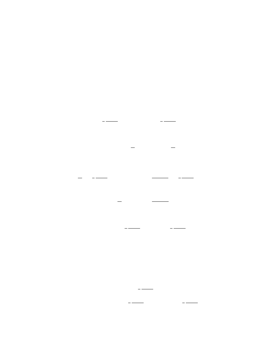
Now, it’s not hard to see that if A and B are operators whose commutator is a
number a, then
[A, B] = a,
[A, B
2
] = 2aB,
[A, B
3
] = 3aB
2
,
..
.
[A, B
n
] = naB
n−1
.
Hence,
·
J(x),
µ
1
i
δ
δJ(y)
n
¸
= iδ(x − y)n
µ
1
i
δ
δJ(y)
n−1
.
(116)
Assume that L
int
(φ) possesses a Taylor series expansion
L
int
(φ) = c
0
+ c
1
φ +
1
2!
c
2
φ
2
+ · · · =
∞
X
n=0
1
n!
c
n
φ
n
.
(117)
Since [A, (B + C)] = [A, B] + [A, C], we can write
"
J(x),
∞
X
n=0
1
n!
c
n
µ
1
i
δ
δJ(y)
n
#
= iδ(x − y)
∞
X
n=1
1
(n − 1)!
c
n
µ
1
i
δ
δJ(y)
n−1
.
(118)
But
L
0
int
(φ) =
∞
X
n=0
n
n!
c
n
φ
n−1
=
∞
X
n=1
1
(n − 1)!
c
n
φ
n−1
.
(119)
Using this an integrating (118) with respect to y gives
·
J(x), i
Z
d
4
y L
int
µ
1
i
δ
δJ(y)
¶¸
= −L
0
int
µ
1
i
δ
δJ(x)
.
(120)
where we have scaled L
int
by i. Finally, note that the Hausdorff formula gives
e
−B
Ae
B
= A + [A, B]
(121)
when [A, B] is a number. Putting (120) into (121) with A = J(x) and B =
i
R
d
4
y L
int
(−iδ/δJ(y)) yields (113).
Using our assumed form for Z[J] (112) and the identity (113) we get
J(x)Z[J] = N J(x) exp
·
i
Z
d
4
y L
int
µ
1
i
δ
δJ(y)
¶¸
Z
0
[J]
= N exp
·
i
Z
d
4
y L
int
µ
1
i
δ
δJ(y)
¶¸ ·
J(x) − L
0
int
µ
1
i
δ
δJ(x)
¶¸
Z
0
[J]
27

= N exp
·
i
Z
d
4
y L
int
µ
1
i
δ
δJ(y)
¶¸
(¤
x
+ m
2
)
1
i
δ
δJ(x)
Z
0
[J]
−L
0
int
µ
1
i
δ
δJ(x)
N exp
·
i
Z
d
4
y L
int
µ
1
i
δ
δJ(y)
¶¸
Z
0
[J]
= (¤
x
+ m
2
)
1
i
δZ[J]
δJ(x)
− L
0
int
µ
1
i
δ
δJ(x)
Z[J].
In going from the second to the third line, we have used the differential equation
satisfied by Z
0
[J] (99). This result is just the differential equation (111), which
confirms that we can write
Z[J] =
exp
h
i
R
d
4
x L
int
³
1
i
δ
δJ(x)
´i
Z
0
[J]
exp
h
i
R
d
4
x L
int
³
1
i
δ
δJ(x)
´i
Z
0
[J]
¯
¯
¯
J=0
(122)
where we have
Z
0
[J] = exp
·
−
i
2
Z
J(x)∆
F
(x − y)J(y) d
4
x d
4
y
¸
.
(123)
With these two equations, we have succeeding in writing down the generating func-
tional entirely in terms of the source J and the Feynman propagator ∆
F
.
7
φ
4
and φ
3
theory
We would like to demonstrate the calculation of the generating functional Z[J] and
some n-point functions in the case of self-interacting φ
4
and φ
3
theory. We follow
section 6.5 of Ryder [1] and chapter 2 of Popov [4]. We first consider φ
4
theory,
which has the interacting Lagrangian:
L
int
(φ) = −
λ
4!
φ
4
.
(124)
It goes without saying that λ is small. The generating functional Z
4
[J] for φ
4
is
Z
4
[J] =
exp
·
−
iλ
4!
R
d
4
z
³
1
i
δ
δJ(z)
´
4
¸
Z
0
[J]
exp
·
−
iλ
4!
R
d
4
z
³
1
i
δ
δJ(x)
´
4
¸
Z
0
[J]
¯
¯
¯
J=0
(125)
The numerator of Z
4
[J] is, to first order in λ, is:
num Z
4
[J] =
"
1 −
iλ
4!
Z
d
4
z
µ
1
i
δ
δJ(z)
4
+ · · ·
#
Z
0
[J].
(126)
28

Performing the functional differentiation, we obtain
num Z
4
[J] =
(
1 −
iλ
4!
Z
d
4
z
"
−3∆
2
F
(0) + 6i∆
F
(0)
µZ
d
4
x ∆
F
(z − x)J(x)
2
+
µZ
d
4
x ∆
F
(z − x)J(x)
4
#
+ · · ·
)
Z
0
[J],
(127)
where we have written ∆
F
(z − z) = ∆
F
(0)
6
. We also get
denom Z
4
[J] = num Z
4
[J]
¯
¯
¯
¯
J=0
=
½
1 −
iλ
4!
Z
d
4
z
£
−3∆
2
F
(0)
¤
+ · · ·
¾
Z
0
[J].
(128)
Putting the two results together yields, to order λ, we have:
Z
4
[J] =
(
1 −
iλ
4!
Z
d
4
z
"
6i∆
F
(0)
µZ
d
4
x ∆
F
(z − x)J(x)
2
+
µZ
d
4
x ∆
F
(z − x)J(x)
4
#
+ · · ·
)
Z
0
[J],
(129)
Now, let’s do the same thing for φ
3
theory, where the interacting Lagrangian is
L
int
(φ) = −
λ
3!
φ
3
.
(130)
The numerator of the generating functional is
num Z
3
[J] = exp
"
−
iλ
3!
Z
d
4
z
µ
1
i
δ
δJ(z)
3
#
Z
0
[J].
(131)
Expanding to order λ, we get
num Z
3
[J] =
½
1 −
iλ
3!
Z
d
4
z
·
−3i∆
F
(0)
Z
d
4
x ∆
F
(z − x)J(x)
−
µZ
d
4
x ∆
F
(z − x)J(x)
3
#
+ · · ·
)
Z
0
[J].
(132)
If we set J = 0, the above reduces to unity. So, the denominator of Z
3
[J] is 1, to
first order in λ, which yields:
Z
3
[J] =
½
1 −
iλ
3!
Z
d
4
z
·
−3i∆
F
(0)
Z
d
4
x ∆
F
(z − x)J(x)
−
µZ
d
4
x ∆
F
(z − x)J(x)
3
#
+ · · ·
)
Z
0
[J].
(133)
6
The Feynman propagator evaluated at zero is, of course, infinite. It’s inclusion in the generating
functional represents the infinite self-energy of particles in the theory and must be regulated by
renormalization, which we will not consider here.
29
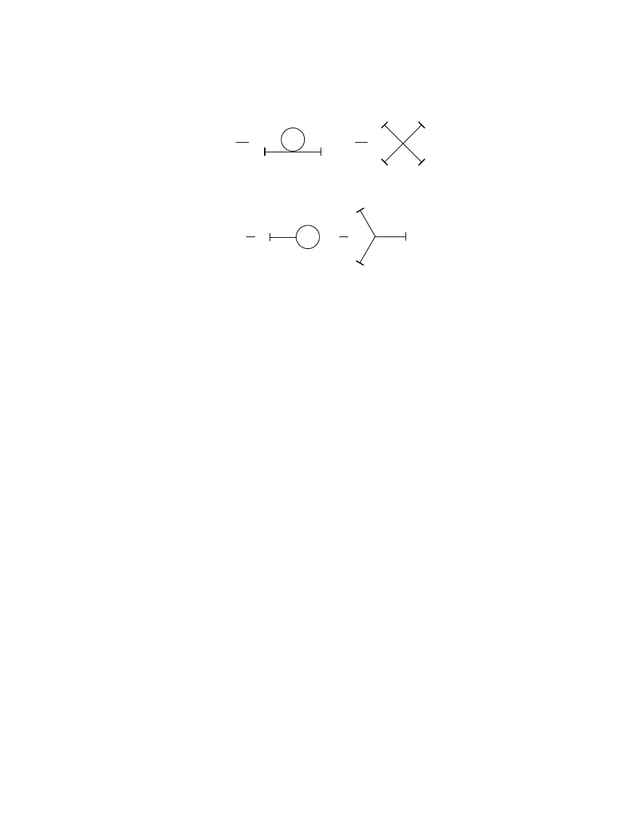
…
il
6
-
+
l
2
x
1
z
+
Z J
[ ] = 1
3
z
x
1
x
2
x
3
l
4
+
x
1
x
2
z
z
…
+
Z J
[ ] = 1
4
x
1
x
2
x
3
x
4
il
24
-
Figure 9: Pictorial representation of the generating functional for φ
4
and φ
3
theory
respectively
We can represent the two generating functionals Z
4
[J] and Z
3
[J] diagrammati-
cally with the following Feynman rules:
1. The spacetime point z
i
is associated with internal points, all other variables
go with external points (recall that z
i
is the coordinate that occurred in the
interacting Lagrangian).
2. A line between x and z comes with a propagator ∆
F
(x − z).
3. Each internal point comes with a factor of iλ/4! for φ
4
theory, iλ/3! for φ
3
theory.
4. External points x come with a factor J(x).
5. Terms of the form ∆
F
(0) represent closed loops, or propagators who begin
and end at the same point, joined to internal points.
6. All spacetime points are integrated over.
7. Each term in the series is multiplied by the free particle propagator Z
0
[J].
These rules give the pictures in figure 9 for Z
4
[J] and Z
3
[J]. These diagrams stress
the general structure of the two theories. Because of the power of 4 in the interact-
ing Lagrangian in φ
4
theory, the vertices in the associated Feynman diagrams are
attached to 4 legs. Similarly, the vertices in φ
3
theory are attached to 3 legs. A
peculiarity of φ
3
theory is the diagram with only one external point. As we will see
below, this gives rise to a one point correlation function which means that particles
in φ
3
can spontaneously self-destruct.
30
l
2
-
x
1
x
2
z
x
1
x
2
…
+
i
il
4
x
1
z
…
+
Figure 10: Pictorial representation of the two-point function h0|T [φ(x
1
)φ(x
2
)]|0i
4
for
φ
4
theory (top) and of the one-point function h0|T [φ(x
1
)]|0i
3
for φ
3
theory (bottom)
Let’s calculate the 2-point function for φ
4
theory:
h0|T [φ(x
1
)φ(x
2
)]|0i
4
= −
δ
2
Z
4
[J]
δJ(x
2
)δJ(x
1
)
¯
¯
¯
¯
J=0
.
(134)
The functional differentiation is easy to do from (129) using the our previously
derived formulae for derivatives of the free field propagator (87) – (90). The result
is
h0|T [φ(x
1
)φ(x
2
)]|0i
4
= i∆
F
(x
1
− x
2
) −
λ
2
∆
F
(0)
Z
d
4
z ∆
F
(x
1
− z)∆
F
(z − x
2
)
+ O(λ
2
).
(135)
This can be turned into a Feynman diagram, as in figure 10, using rules similar
to the ones for Z[J], except now the only the internal points are integrated over.
Figure 10 shows how the amplitude for the creation of a particle at point x
1
and its
later destruction at x
2
is modified by an (infinite) loop diagram to first-order in λ
in φ
4
theory.
Now, let’s get the 2-point function in φ
3
theory. It is simply calculated
h0|T [φ(x
1
)φ(x
2
)]|0i
3
= −
δ
2
Z
3
[J]
δJ(x
2
)δJ(x
1
)
¯
¯
¯
¯
J=0
= i∆
F
(x
1
− x
2
) + O(λ
2
).
(136)
This isn’t terribly interesting, we see that there are no corrections to the free field
result to this level in perturbation theory. We shouldn’t be surprised, there is no
way to connect to external lines to a single vertex if the vertex must be attached
to three lines. However, there is a way to connect a vertex to one external line and
one internal line, as shown in figure 10. This is borne out by the calculation of the
one-point function:
h0|T [φ(x
1
)]|0i
3
= −i
δ
2
Z
3
[J]
δJ(x
1
)
¯
¯
¯
¯
J=0
=
iλ
4
∆
F
(0)
Z
d
4
z ∆
F
(z − x
1
) + O(λ
2
).
(137)
31
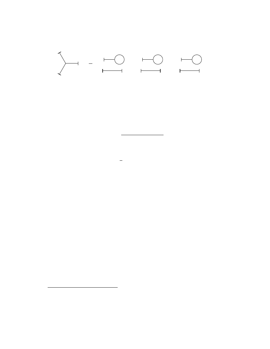
…
l
4
+
+
+
+
x
1
z
x
2
x
3
x
2
z
x
3
x
1
x
3
z
x
1
x
2
-l
z
x
1
x
2
x
3
(
(
Figure 11: Pictorial representation of h0|T [φ(x
1
)φ(x
2
)φ(x
3
)]|0i
3
, the three point
function, for φ
3
theory
Certainly a strange beast, this represents the amplitude of a particle being sponta-
neously created out of the vacuum, all by itself
7
. We can also calculate the three
point function
h0|T [φ(x
1
)φ(x
2
)φ(x
3
)]|0i
3
= i
δ
2
Z
3
[J]
δJ(x
3
)δJ(x
2
)δJ(x
1
)
¯
¯
¯
¯
J=0
= −λ
Z
d
4
z ∆
F
(z − x
1
)∆
F
(z − x
2
)∆
F
(z − x
3
)
+
λ
4
∆
F
(0)
Z
d
4
z [∆
F
(z − x
1
)∆
F
(x
2
− x
3
)
+ ∆
F
(z − x
2
)∆
F
(x
3
− x
1
)
+ ∆
F
(z − x
3
)∆
F
(x
1
− x
2
)].
(138)
The first integral involves all the external legs attached to the same point, i.e. two
particles merging into one or one particle splitting in two. The second integral
is the product of free 2-point functions and the 1-point function we have already
calculated. The diagram is in figure 11.
We have hence shown how the generating functional and n-point functions can
be found from simple functional differentiation of equations (122) and (123) and
expressed in terms of Feynman diagrams. These diagrams can be converted into
scattering amplitudes via the LSZ reduction formula
8
:
hp
1
, . . . , p
n
, +∞|q
1
, . . . , q
m
, −∞i = disconnected terms
+ (i)
n+m
Z
dy
1
· · · dy
n
dx
1
· · · dx
m
× e
i(p
1
·y
1
+···+p
n
·y
n
−q
1
·x
1
−···−q
m
·x
m
)
× (¤
y
1
+ m
2
) · · · (¤
y
n
+ m
2
)
× (¤
x
1
+ m
2
) · · · (¤
x
m
+ m
2
)
× h0|T [φ(y
1
) · · · φ(y
n
)φ(x
1
) . . . φ(x
m
)]|0i.
7
However, such a process would be forbidden on energy grounds
8
cf. PHYS 703 March 16, 2000. Brown [3] claims that this formula can be obtained via path
integral methods, by he presents a proof using the canonical formalism.
32

In practice, these scattering amplitudes are the only meaningful quantities in quan-
tum field theory since they are the only things that can be directly measured. So,
having arrived at a point where we can calculate hp
1
, . . . , p
n
, +∞|q
1
, . . . , q
m
, −∞i
using the generating functional, we have completed our formulation of self-interacting
field theories in terms of path integrals.
More complicated theories, such as QED, can be quantized in terms of path-
integrals, but there are several issues that need to be addressed when writing down
Z[J] for gauge fields. One finds that Z[J] is infinite for gauge fields A
α
, because the
R
[dA
α
] integration includes an infinite number of contributions from fields related
by a simple gauge transformation. The resolution is the addition of gauge fixing
terms to the Lagrangian and the appearance of non-physical “ghost fields”. Such
things are beyond the scope of this paper.
8
Conclusions
We have demonstrated how quantum mechanics can be formulated in terms of the
propagator that represents the amplitude of a particle travels from some initial
position to some final position. We have determined the form of the propagator to
be a sum over paths of the amplitudes associated with the particle traveling along
a given trajectory. The amplitude associated with the path q(t) was shown to be
e
iS[q]
, where S[q] is the classical Lagrangian. We used this form of the propagator
to derive Feynman rules for the S
f i
matrix in non-relativistic scattering problems.
Then, we showed that by adding a source J(t) to the Lagrangian and rotating the
time axis in the complex plane, the propagator Z[J] reduces to the ground state-
to-ground state transition amplitude. Functional derivatives of Z[J] with respect
to the source J(t) were shown to give the time-ordered product of configuration
operators q(t).
We generalized the propagator to free scalar fields and expanded Z[J] in terms
of Feynman diagrams by expressing it in terms of the Feynman propagator and
the source J(x). In the process, we derived some n-point correlation functions by
differentiating Z[J]. We discussed how the rotation of the time axis needed to
isolate the vacuum-to-vacuum transition probability is directly responsible for the
prominent role that the Feynman propagator plays in field theory. We developed a
formalism to deal with self-interacting fields and expressed Z[J] entirely in terms of
∆
F
(x), J(x), and the series expansion of the interacting Lagrangian. For both φ
4
and φ
3
theory, we expressed Z[J] and some n-point functions in terms of Feynman
diagrams. Since the scattering problem is essentially solved once the procedure
for calculating n-point functions is specified (ignoring issues of renormalization), we
have hence shown how all of the theory of self-interacting scalar fields can be derived
from path integrals.
33

References
[1] Lewis H. Ryder. Quantum Field Theory, 2
nd
ed.. Cambridge: 1996.
[2] Gordon Baym. Lecture Notes on Quantum Mechanics. Benjamin/Cummings:
1969.
[3] Lowell S. Brown. Quantum Field Theory. Cambridge: 1992.
[4] Viktor N. Poppv. Functional Integrals in Quantum Field Theory and Statistical
Physics. Reidel: 1983.
34
Wyszukiwarka
Podobne podstrony:
Feynman s Path Integral in Quantum Theory
Modanese Inertial Mass and Vacuum Fluctuations in Quantum Field Theory (2003)
Reid H Solved problems from Peskin Schroeder QFT, chapters 2 to 5 (web draft, 2002)(40s) PQft
Srednicki M Quantum field theory, part 2 spin one half (web draft, 2005)(146s) PQtb
Alvarez Gaume L , Introductory Lectures on Quantum Field Theory
Norbury Quantum field theory (Wisconsin lecture notes, 2000)(107s)
Quantum field theory
Rajeev S G Geometrical methods in physics (lecture notes, web draft, 2004)(97s)
Walet N Mathematics for Physicists (web draft, 2002)(81s) MCet
Rajeev S G Advanced classical mechanics chaos (Rochester lecture notes, web draft, 2002)(100s) PCtm
Walet N Further Maths 2C1 Lecture Notes(web draft, 2002)(79s) MCde
Field M , Nicol M Ergodic theory of equivariant diffeomorphisms (web draft, 2004)(94s) PD
Petkov Nature of force acting on charged classical particle deviated from its geodesic path in grav
Escobedo M , Mischler S , Valle M A Homogeneous Boltzmann equation in quantum relativistic kinetic t
Haisch et al Advances in the Proposed Electromagnetic Zero Point Field Theory of Inertia (1998)
Margaret May Business Process Management Integration in a Web Enabled Environment 2003 (By Laxxu
Clinical Advances in Cognitive Psychotherapy Theory and Application R Leahy, E Dowd (Springer, 200
Freitag Several complex variables local theory (lecture notes, web draft, 2001)(74s) MCc
więcej podobnych podstron