
arXiv:hep-th/0510040v3 12 Feb 2010
Introductory Lectures on Quantum Field Theory
∗
Luis ´
Alvarez-Gaum´e
a,
†
and Miguel A. V´azquez-Mozo
b, c,
‡
a
Physics Department, Theory Division, CERN, CH-1211 Geneva 23, Switzerland
b
Departamento de F´ısica Fundamental, Universidad de Salamanca, Plaza de la Merced s/n,
E-37008 Salamanca, Spain
c
Instituto Universitario de F´ısica Fundamental y Matem´aticas (IUFFyM), Universidad de
Salamanca, Salamanca, Spain
Abstract
In these lectures we present a few topics in Quantum Field Theory in detail.
Some of them are conceptual and some more practical. They have been
selected because they appear frequently in current applications to Particle
Physics and String Theory.
∗
Based on lectures delivered by L.A.-G. at the 3rd. CERN-CLAF School of High-Energy Physics, Malarg ¨ue (Ar-
gentina), February 27th-March 12th, 2005 and at the 5th. CERN-CLAF School of High-Energy Physics, Medell´ın
(Colombia), 15th-28th March, 2009
†
Luis.Alvarez-Gaume@cern.ch
‡
Miguel.Vazquez-Mozo@cern.ch, vazquez@usal.es
1

C
ONTENTS
1
Introduction
3
1.1
A note about notation . . . . . . . . . . . . . . . . . . . . . . . . . . . . . . . . . . .
4
2
Why do we need Quantum Field Theory after all?
4
3
From classical to quantum fields
10
3.1
Canonical quantization . . . . . . . . . . . . . . . . . . . . . . . . . . . . . . . . . .
16
3.2
The Casimir effect
. . . . . . . . . . . . . . . . . . . . . . . . . . . . . . . . . . . .
19
4
Theories and Lagrangians
21
4.1
Representations of the Lorentz group . . . . . . . . . . . . . . . . . . . . . . . . . . .
21
4.2
Spinors . . . . . . . . . . . . . . . . . . . . . . . . . . . . . . . . . . . . . . . . . .
23
4.3
Gauge fields . . . . . . . . . . . . . . . . . . . . . . . . . . . . . . . . . . . . . . . .
29
4.4
Understanding gauge symmetry
. . . . . . . . . . . . . . . . . . . . . . . . . . . . .
36
5
Towards computational rules: Feynman diagrams
43
5.1
Cross sections and S-matrix amplitudes . . . . . . . . . . . . . . . . . . . . . . . . .
43
5.2
Feynman rules . . . . . . . . . . . . . . . . . . . . . . . . . . . . . . . . . . . . . . .
46
5.3
An example: Compton scattering . . . . . . . . . . . . . . . . . . . . . . . . . . . . .
52
6
Symmetries
56
6.1
Noether’s theorem . . . . . . . . . . . . . . . . . . . . . . . . . . . . . . . . . . . . .
56
6.2
Symmetries in the quantum theory . . . . . . . . . . . . . . . . . . . . . . . . . . . .
59
7
Anomalies
66
7.1
Axial anomaly . . . . . . . . . . . . . . . . . . . . . . . . . . . . . . . . . . . . . . .
66
7.2
Chiral symmetry in QCD . . . . . . . . . . . . . . . . . . . . . . . . . . . . . . . . .
72
8
Renormalization
79
8.1
Removing infinities . . . . . . . . . . . . . . . . . . . . . . . . . . . . . . . . . . . .
79
8.2
The beta-function and asymptotic freedom . . . . . . . . . . . . . . . . . . . . . . . .
83
8.3
The renormalization group . . . . . . . . . . . . . . . . . . . . . . . . . . . . . . . .
89
9
Special topics
97
9.1
Creation of particles by classical fields . . . . . . . . . . . . . . . . . . . . . . . . . .
97
9.2
Supersymmetry . . . . . . . . . . . . . . . . . . . . . . . . . . . . . . . . . . . . . . 103
2

1
Introduction
These notes summarize the lectures presented at the 2005 CERN-CLAF school in Malarg¨ue, Ar-
gentina and the 2009 CERN-CLAF school in Medell´ın, Colombia. The audience in both occasions
was composed to a large extent by students in experimental High Energy Physics with an important
minority of theorists. In nearly ten hours it is quite difficult to give a reasonable introduction to a
subject as vast as Quantum Field Theory. For this reason the lectures were intended to provide a re-
view of those parts of the subject to be used later by other lecturers. Although a cursory acquaitance
with th subject of Quantum Field Theory is helpful, the only requirement to follow the lectures it is
a working knowledge of Quantum Mechanics and Special Relativity.
The guiding principle in choosing the topics presented (apart to serve as introductions to later
courses) was to present some basic aspects of the theory that present conceptual subtleties. Those
topics one often is uncomfortable with after a first introduction to the subject. Among them we have
selected:
- The need to introduce quantum fields, with the great complexity this implies.
- Quantization of gauge theories and the rˆole of topology in quantum phenomena. We have in-
cluded a brief study of the Aharonov-Bohm effect and Dirac’s explanation of the quantization
of the electric charge in terms of magnetic monopoles.
- Quantum aspects of global and gauge symmetries and their breaking.
- Anomalies.
- The physical idea behind the process of renormalization of quantum field theories.
- Some more specialized topics, like the creation of particle by classical fields and the very
basics of supersymmetry.
These notes have been written following closely the original presentation, with numerous
clarifications. Sometimes the treatment given to some subjects has been extended, in particular the
discussion of the Casimir effect and particle creation by classical backgrounds. Since no group
theory was assumed, we have included an Appendix with a review of the basics concepts.
By lack of space and purpose, few proofs have been included. Instead, very often we illustrate
a concept or property by describing a physical situation where it arises. Full details and proofs
can be found in the many textbooks in the subject, and in particular in the ones provided in the
bibliography [1–10]. Specially modern presentations, very much in the spirit of these lectures, can
be found in references [4, 5, 9, 10]. We should nevertheless warn the reader that we have been a bit
cavalier about references. Our aim has been to provide mostly a (not exhaustive) list of reference
for further reading. We apologize to those authors who feel misrepresented.
Acknowlegments. It is a great pleasure to thank the organizers of the CERN-CLAF 2005 and
2009 Schools, and in particular Teresa Dova, Marta Losada and Enrico Nardi, for the opportunity to
present this material, and for the wonderful atmosphere they created during the schools. The work
of M.A.V.-M. has been partially supported by Spanish Science Ministry Grants FPA2002-02037,
FPA2005-04823 and BFM2003-02121.
3
1.1
A note about notation
Before starting it is convenient to review the notation used. Through these notes we will be using
the metric
η
µν
= diag (1,
−1, −1, −1). Derivatives with respect to the four-vector x
µ
= (ct, ~x) will
be denoted by the shorthand
∂
µ
≡
∂
∂x
µ
=
1
c
∂
∂t
, ~
∇
.
(1.1)
As usual space-time indices will be labelled by Greek letters (
µ, ν, . . . = 0, 1, 2, 3) while Latin
indices will be used for spatial directions (
i, j, . . . = 1, 2, 3). In many expressions we will use the
notation
σ
µ
= (1, σ
i
) where σ
i
are the Pauli matrices
σ
1
=
0 1
1 0
,
σ
2
=
0
−i
i
0
,
σ
3
=
1
0
0
−1
.
(1.2)
Sometimes we use of the Feynman’s slash notation
/a = γ
µ
a
µ
. Finally, unless stated otherwise, we
work in natural units ~
= c = 1.
2
Why do we need Quantum Field Theory after all?
In spite of the impressive success of Quantum Mechanics in describing atomic physics, it was
immediately clear after its formulation that its relativistic extension was not free of difficulties.
These problems were clear already to Schr¨odinger, whose first guess for a wave equation of a free
relativistic particle was the Klein-Gordon equation
∂
2
∂t
2
− ∇
2
+ m
2
ψ(t, ~x) = 0.
(2.1)
This equation follows directly from the relativistic “mass-shell” identity
E
2
= ~p
2
+ m
2
using the
correspondence principle
E
→ i
∂
∂t
,
~p
→ −i~∇.
(2.2)
Plane wave solutions to the wave equation (2.1) are readily obtained
ψ(t, ~x) = e
−ip
µ
x
µ
= e
−iEt+i~p·~x
with
E =
±ω
p
≡ ±
p
~p
2
+ m
2
.
(2.3)
In order to have a complete basis of functions, one must include plane wave with both
E > 0 and
E < 0. This implies that given the conserved current
j
µ
=
i
2
ψ
∗
∂
µ
ψ
− ∂
µ
ψ
∗
ψ
,
(2.4)
its time-component is
j
0
= E and therefore does not define a positive-definite probability density.
4
Energy
m
0
−m
Fig. 1: Spectrum of the Klein-Gordon wave equation
A complete, properly normalized, continuous basis of solutions of the Klein-Gordon equation
(2.1) labelled by the momentum
~p can be defined as
f
p
(t, ~x) =
1
(2π)
2
p
2ω
p
e
−iω
p
t
+i~
p
·~x
,
f
−p
(t, ~x) =
1
(2π)
2
p
2ω
p
e
iω
p
t
−i~p·~x
.
(2.5)
Given the inner product
hψ
1
|ψ
2
i = i
Z
d
3
x
ψ
∗
1
∂
0
ψ
2
− ∂
0
ψ
∗
1
ψ
2
the states (2.5) form an orthonormal basis
hf
p
|f
p
′
i = δ(~p − ~p
′
),
hf
−p
|f
−p
′
i = −δ(~p − ~p
′
),
(2.6)
hf
p
|f
−p
′
i = 0.
(2.7)
The wave functions
f
p
(t, x) describes states with momentum ~p and energy given by ω
p
=
p
~p
2
+ m
2
. On the other hand, the states
|f
−p
i not only have a negative scalar product but they
actually correspond to negative energy states
i∂
0
f
−p
(t, ~x) =
−
p
~p
2
+ m
2
f
−p
(t, ~x).
(2.8)
5
Therefore the energy spectrum of the theory satisfies
|E| > m and is unbounded from below (see
Fig. 1). Although in a case of a free theory the absence of a ground state is not necessarily a fatal
problem, once the theory is coupled to the electromagnetic field this is the source of all kinds of
disasters, since nothing can prevent the decay of any state by emission of electromagnetic radiation.
The problem of the instability of the “first-quantized” relativistic wave equation can be heuris-
tically tackled in the case of spin-
1
2
particles, described by the Dirac equation
−iβ
∂
∂t
+ ~
α
· ~
∇ − m
ψ(t, ~x) = 0,
(2.9)
where
~
α and β are 4
× 4 matrices
α
i
=
0
iσ
i
−iσ
i
0
,
β =
0 1
1
0
,
(2.10)
with
σ
i
the Pauli matrices, and the wave function
ψ(t, ~x) has four components. The wave equation
(2.9) can be thought of as a kind of “square root” of the Klein-Gordon equation (2.1), since the latter
can be obtained as
−iβ
∂
∂t
+ ~
α
· ~
∇ − m
†
−iβ
∂
∂t
+ ~
α
· ~
∇ − m
ψ(t, ~x) =
∂
2
∂t
2
− ∇
2
+ m
2
ψ(t, ~x). (2.11)
An analysis of Eq. (2.9) along the lines of the one presented above for the Klein-Gordon
equation leads again to the existence of negative energy states and a spectrum unbounded from
below as in Fig. 1. Dirac, however, solved the instability problem by pointing out that now the
particles are fermions and therefore they are subject to Pauli’s exclusion principle. Hence, each
state in the spectrum can be occupied by at most one particle, so the states with
E = m can be made
stable if we assume that all the negative energy states are filled.
If Dirac’s idea restores the stability of the spectrum by introducing a stable vacuum where all
negative energy states are occupied, the so-called Dirac sea, it also leads directly to the conclusion
that a single-particle interpretation of the Dirac equation is not possible. Indeed, a photon with
enough energy (
E > 2m) can excite one of the electrons filling the negative energy states, leaving
behind a “hole” in the Dirac see (see Fig. 2). This hole behaves as a particle with equal mass
and opposite charge that is interpreted as a positron, so there is no escape to the conclusion that
interactions will produce pairs particle-antiparticle out of the vacuum.
In spite of the success of the heuristic interpretation of negative energy states in the Dirac
equation this is not the end of the story. In 1929 Oskar Klein stumbled into an apparent paradox
when trying to describe the scattering of a relativistic electron by a square potential using Dirac’s
wave equation [11] (for pedagogical reviews see [12, 13]). In order to capture the essence of the
problem without entering into unnecessary complication we will study Klein’s paradox in the con-
text of the Klein-Gordon equation.
Let us consider a square potential with height
V
0
> 0 of the type showed in Fig. 3. A solution
to the wave equation in regions I and II is given by
ψ
I
(t, x) = e
−iEt+ip
1
x
+ Re
−iEt−ip
1
x
,
ψ
II
(t, x) = T e
−iEt+p
2
x
,
(2.12)
6
Energy
m
−m
particle
antiparticle (hole)
photon
Dirac Sea
Fig. 2: Creation of a particle-antiparticle pair in the Dirac see picture
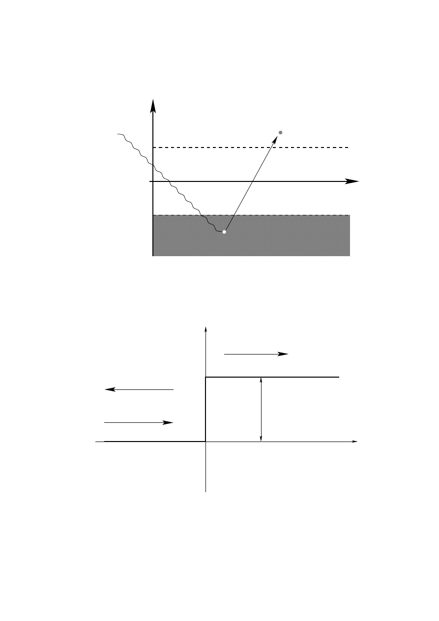
x
V(x)
V
0
Incoming
Reflected
Transmited
Fig. 3: Illustration of the Klein paradox.
7
where the mass-shell condition implies that
p
1
=
√
E
2
− m
2
,
p
2
=
p
(E
− V
0
)
2
− m
2
.
(2.13)
The constants
R and T are computed by matching the two solutions across the boundary x = 0.
The conditions
ψ
I
(t, 0) = ψ
II
(t, 0) and ∂
x
ψ
I
(t, 0) = ∂
x
ψ
II
(t, 0) imply that
T =
2p
1
p
1
+ p
2
,
R =
p
1
− p
2
p
1
+ p
2
.
(2.14)
At first sight one would expect a behavior similar to the one encountered in the nonrelativistic
case. If the kinetic energy is bigger than
V
0
both a transmitted and reflected wave are expected,
whereas when the kinetic energy is smaller than
V
0
one only expect to find a reflected wave, the
transmitted wave being exponentially damped within a distance of a Compton wavelength inside
the barrier.
Indeed this is what happens if
E
− m > V
0
. In this case both
p
1
and
p
2
are real and we have a
partly reflected, and a partly transmitted wave. In the same way, if
E
−m < V
0
and
E
−m < V
0
−2m
then
p
2
is imaginary and there is total reflection.
However, in the case when
V
0
> 2m and the energy is in the range V
0
− 2m < E − m < V
0
a
completely different situation arises. In this case one finds that both
p
1
and
p
2
are real and therefore
the incoming wave function is partially reflected and partially transmitted across the barrier. This is
a shocking result, since it implies that there is a nonvanishing probability of finding the particle at
any point across the barrier with negative kinetic energy (
E
− m − V
0
< 0)! This weird result is
known as Klein’s paradox.
As with the negative energy states, the Klein paradox results from our insistence in giving a
single-particle interpretation to the relativistic wave function. Actually, a multiparticle analysis of
the paradox [12] shows that what happens when
E
− m > V
0
− 2m is that the reflection of the
incoming particle by the barrier is accompanied by the creation of pairs particle-antiparticle out of
the energy of the barrier (notice that for this to happen it is required that
V
0
> 2m, the threshold for
the creation of a particle-antiparticle pair).
Actually, this particle creation can be understood by noticing that the sudden potential step in
Fig. 3 localizes the incoming particle with mass
m in distances smaller than its Compton wavelength
λ =
1
m
. This can be seen by replacing the square potential by another one where the potential varies
smoothly from
0 to V
0
> 2m in distances scales larger than 1/m. This case was worked out by
Sauter shortly after Klein pointed out the paradox [14]. He considered a situation where the regions
with
V = 0 and V = V
0
are connected by a region of length
d with a linear potential V (x) =
V
0
x
d
.
When
d >
1
m
he found that the transmission coefficient is exponentially small
1
.
The creation of particles is impossible to avoid whenever one tries to locate a particle of mass
m within its Compton wavelength. Indeed, from Heisenberg uncertainty relation we find that if
∆x
∼
1
m
, the fluctuations in the momentum will be of order
∆p
∼ m and fluctuations in the energy
of order
∆E
∼ m
(2.15)
1
In section (9.1) we will see how, in the case of the Dirac field, this exponential behavior can be associated with the
creation of electron-positron pairs due to a constant electric field (Schwinger effect).
8
00000
00000
00000
00000
00000
00000
00000
11111
11111
11111
11111
11111
11111
11111
0000
0000
0000
0000
0000
0000
1111
1111
1111
1111
1111
1111
R
1
R
2
x
t
Fig. 4: Two regions R
1
, R
2
that are causally disconnected.
can be expected. Therefore, in a relativistic theory, the fluctuations of the energy are enough to
allow the creation of particles out of the vacuum. In the case of a spin-
1
2
particle, the Dirac sea
picture shows clearly how, when the energy fluctuations are of order
m, electrons from the Dirac
sea can be excited to positive energy states, thus creating electron-positron pairs.
It is possible to see how the multiparticle interpretation is forced upon us by relativistic invari-
ance. In non-relativistic Quantum Mechanics observables are represented by self-adjoint operator
that in the Heisenberg picture depend on time. Therefore measurements are localized in time but
are global in space. The situation is radically different in the relativistic case. Because no signal
can propagate faster than the speed of light, measurements have to be localized both in time and
space. Causality demands then that two measurements carried out in causally-disconnected regions
of space-time cannot interfere with each other. In mathematical terms this means that if
O
R
1
and
O
R
2
are the observables associated with two measurements localized in two causally-disconnected
regions
R
1
,
R
2
(see Fig. 4), they satisfy
[
O
R
1
,
O
R
2
] = 0,
if
(x
1
− x
2
)
2
< 0, for all x
1
∈ R
1
,
x
2
∈ R
2
.
(2.16)
Hence, in a relativistic theory, the basic operators in the Heisenberg picture must depend on
the space-time position
x
µ
. Unlike the case in non-relativistic quantum mechanics, here the position
~x is not an observable, but just a label, similarly to the case of time in ordinary quantum mechanics.
Causality is then imposed microscopically by requiring
[
O(x), O(y)] = 0,
if
(x
− y)
2
< 0.
(2.17)
A smeared operator
O
R
over a space-time region
R can then be defined as
O
R
=
Z
d
4
x
O(x) f
R
(x)
(2.18)
9
where
f
R
(x) is the characteristic function associated with R,
f
R
(x) =
1
x
∈ R
0
x /
∈ R
.
(2.19)
Eq. (2.16) follows now from the microcausality condition (2.17).
Therefore, relativistic invariance forces the introduction of quantum fields. It is only when
we insist in keeping a single-particle interpretation that we crash against causality violations. To
illustrate the point, let us consider a single particle wave function
ψ(t, ~x) that initially is localized
in the position
~x = 0
ψ(0, ~x) = δ(~x).
(2.20)
Evolving this wave function using the Hamiltonian
H =
√
−∇
2
+ m
2
we find that the wave func-
tion can be written as
ψ(t, ~x) = e
−it
√
−∇
2
+m
2
δ(~x) =
Z
d
3
k
(2π)
3
e
i~
k
·~x−it
√
k
2
+m
2
.
(2.21)
Integrating over the angular variables, the wave function can be recast in the form
ψ(t, ~x) =
1
2π
2
|~x|
Z
∞
−∞
k dk e
ik
|~x|
e
−it
√
k
2
+m
2
.
(2.22)
The resulting integral can be evaluated using the complex integration contour
C shown in Fig. 5.
The result is that, for any
t > 0, one finds that ψ(t, ~x)
6= 0 for any ~x. If we insist in interpreting the
wave function
ψ(t, ~x) as the probability density of finding the particle at the location ~x in the time t
we find that the probability leaks out of the light cone, thus violating causality.
3
From classical to quantum fields
We have learned how the consistency of quantum mechanics with special relativity forces us to
abandon the single-particle interpretation of the wave function. Instead we have to consider quantum
fields whose elementary excitations are associated with particle states, as we will see below.
In any scattering experiment, the only information available to us is the set of quantum number
associated with the set of free particles in the initial and final states. Ignoring for the moment other
quantum numbers like spin and flavor, one-particle states are labelled by the three-momentum
~p and
span the single-particle Hilbert space
H
1
|~pi ∈ H
1
,
h~p|~p
′
i = δ(~p − ~p
′
) .
(3.1)
The states
{|~pi} form a basis of H
1
and therefore satisfy the closure relation
Z
d
3
p
|~pih~p| = 1
(3.2)
10
k
m
i
C
Fig. 5: Complex contour C for the computation of the integral in Eq. (2.22).
The group of spatial rotations acts unitarily on the states
|~pi. This means that for every rotation
R
∈ SO(3) there is a unitary operator U(R) such that
U(R)|~pi = |R~pi
(3.3)
where
R~p represents the action of the rotation on the vector ~k, (R~p)
i
= R
i
j
k
j
. Using a spectral
decomposition, the momentum operator b
P
i
can be written as
b
P
i
=
Z
d
3
p
|~pi p
i
h~p|
(3.4)
With the help of Eq. (3.3) it is straightforward to check that the momentum operator transforms as
a vector under rotations:
U(R)
−1
b
P
i
U(R) =
Z
d
3
p
|R
−1
~p
i p
i
hR
−1
~p
| = R
i
j
b
P
j
,
(3.5)
where we have used that the integration measure is invariant under SO
(3).
Since, as we argued above, we are forced to deal with multiparticle states, it is convenient to
introduce creation-annihilation operators associated with a single-particle state of momentum
~p
[a(~p), a
†
(~p
′
)] = δ(~p
− ~p
′
),
[a(~p), a(~p
′
)] = [a
†
(~p), a
†
(~p
′
)] = 0,
(3.6)
such that the state
|~pi is created out of the Fock space vacuum |0i (normalized such that h0|0i = 1)
by the action of a creation operator
a
†
(~p)
|~pi = a
†
(~p)
|0i,
a(~p)
|0i = 0 ∀~p.
(3.7)
11
Covariance under spatial rotations is all we need if we are interested in a nonrelativistic theory.
However in a relativistic quantum field theory we must preserve more that SO
(3), actually we
need the expressions to be covariant under the full Poincar´e group ISO
(1, 3) consisting in spatial
rotations, boosts and space-time translations. Therefore, in order to build the Fock space of the
theory we need two key ingredients: first an invariant normalization for the states, since we want a
normalized state in one reference frame to be normalized in any other inertial frame. And secondly
a relativistic invariant integration measure in momentum space, so the spectral decomposition of
operators is covariant under the full Poincar´e group.
Let us begin with the invariant measure. Given an invariant function
f (p) of the four-momen-
tum
p
µ
of a particle of mass
m with positive energy p
0
> 0, there is an integration measure which
is invariant under proper Lorentz transformations
2
Z
d
4
p
(2π)
4
(2π)δ(p
2
− m
2
) θ(p
0
) f (p),
(3.8)
where
θ(x) represent the Heaviside step function. The integration over p
0
can be easily done using
the
δ-function identity
δ[f (x)] =
X
x
i
=zeros of f
1
|f
′
(x
i
)
|
δ(x
− x
i
),
(3.9)
which in our case implies that
δ(p
2
− m
2
) =
1
2p
0
δ
p
0
−
p
~p
2
+ m
2
+
1
2p
0
δ
p
0
+
p
~p
2
+ m
2
.
(3.10)
The second term in the previous expression correspond to states with negative energy and therefore
does not contribute to the integral. We can write then
Z
d
4
p
(2π)
4
(2π)δ(p
2
− m
2
) θ(p
0
) f (p) =
Z
d
3
p
(2π)
3
1
2
p
~p
2
+ m
2
f
p
~p
2
+ m
2
, ~p
.
(3.11)
Hence, the relativistic invariant measure is given by
Z
d
3
p
(2π)
3
1
2ω
p
with
ω
p
≡
p
~p
2
+ m
2
.
(3.12)
Once we have an invariant measure the next step is to find an invariant normalization for the
states. We work with a basis
{|pi} of eigenstates of the four-momentum operator b
P
µ
b
P
0
|pi = ω
p
|pi,
b
P
i
|pi = ~p
i
|pi.
(3.13)
Since the states
|pi are eigenstates of the three-momentum operator we can express them in terms
of the non-relativistic states
|~pi that we introduced in Eq. (3.1)
|pi = N(~p)|~pi
(3.14)
2
The factors of
2π are introduced for later convenience.
12

with
N(~p) a normalization to be determined now. The states
{|pi} form a complete basis, so they
should satisfy the Lorentz invariant closure relation
Z
d
4
p
(2π)
4
(2π)δ(p
2
− m
2
) θ(p
0
)
|pi hp| = 1
(3.15)
At the same time, this closure relation can be expressed, using Eq. (3.14), in terms of the nonrela-
tivistic basis of states
{|~pi} as
Z
d
4
p
(2π)
4
(2π)δ(p
2
− m
2
) θ(p
0
)
|pi hp| =
Z
d
3
p
(2π)
3
1
2ω
p
|N(p)|
2
|~pi h~p|.
(3.16)
Using now Eq. (3.4) for the nonrelativistic states, expression (3.15) follows provided
|N(~p)|
2
= (2π)
3
(2ω
p
).
(3.17)
Taking the overall phase in Eq. (3.14) so that
N(p) is real, we define the Lorentz invariant states
|pi
as
|pi = (2π)
3
2
p
2ω
p
|~pi,
(3.18)
and given the normalization of
|~pi we find the normalization of the relativistic states to be
hp|p
′
i = (2π)
3
(2ω
p
)δ(~p
− ~p
′
).
(3.19)
Although not obvious at first sight, the previous normalization is Lorentz invariant. Although
it is not difficult to show this in general, here we consider the simpler case of 1+1 dimensions where
the two components
(p
0
, p
1
) of the on-shell momentum can be parametrized in terms of a single
hyperbolic angle
λ as
p
0
= m cosh λ,
p
1
= m sinh λ.
(3.20)
Now, the combination
2ω
p
δ(p
1
− p
1′
) can be written as
2ω
p
δ(p
1
− p
1′
) = 2m cosh λ δ(m sinh λ
− m sinh λ
′
) = 2δ(λ
− λ
′
),
(3.21)
where we have made use of the property (3.9) of the
δ-function. Lorentz transformations in 1 + 1
dimensions are labelled by a parameter
ξ
∈ R and act on the momentum by shifting the hyperbolic
angle
λ
→ λ + ξ. However, Eq. (3.21) is invariant under a common shift of λ and λ
′
, so the whole
expression is obviously invariant under Lorentz transformations.
To summarize what we did so far, we have succeed in constructing a Lorentz covariant basis
of states for the one-particle Hilbert space
H
1
. The generators of the Poincar´e group act on the
states
|pi of the basis as
b
P
µ
|pi = p
µ
|pi,
U(Λ)|pi = |Λ
µ
ν
p
ν
i ≡ |Λpi
with
Λ
∈ SO(1, 3).
(3.22)
13
This is compatible with the Lorentz invariance of the normalization that we have checked above
hp|p
′
i = hp|U(Λ)
−1
U(Λ)|p
′
i = hΛp|Λp
′
i.
(3.23)
On
H
1
the operator b
P
µ
admits the following spectral representation
b
P
µ
=
Z
d
3
p
(2π)
3
1
2ω
p
|pi p
µ
hp| .
(3.24)
Using (3.23) and the fact that the measure is invariant under Lorentz transformation, one can easily
show that b
P
µ
transform covariantly under SO
(1, 3)
U(Λ)
−1
b
P
µ
U(Λ) =
Z
d
3
p
(2π)
3
1
2ω
p
|Λ
−1
p
i p
µ
hΛ
−1
p
| = Λ
µ
ν
b
P
ν
.
(3.25)
A set of covariant creation-annihilation operators can be constructed now in terms of the
operators
a(~p), a
†
(~p) introduced above
α(~p)
≡ (2π)
3
2
p
2ω
p
a(~p),
α
†
(~p)
≡ (2π)
3
2
p
2ω
p
a
†
(~p)
(3.26)
with the Lorentz invariant commutation relations
[α(~p), α
†
(~p
′
)] = (2π)
3
(2ω
p
)δ(~p
− ~p
′
),
[α(~p), α(~p
′
)] = [α
†
(~p), α
†
(~p
′
)] = 0.
(3.27)
Particle states are created by acting with any number of creation operators
α(~p) on the Poincar´e
invariant vacuum state
|0i satisfying
h0|0i = 1,
b
P
µ
|0i = 0,
U(Λ)|0i = |0i,
∀Λ ∈ SO(1, 3).
(3.28)
A general one-particle state
|fi ∈ H
1
can be then written as
|fi =
Z
d
3
p
(2π)
3
1
2ω
p
f (~p)α
†
(~p)
|0i,
(3.29)
while a
n-particle state
|fi ∈ H
⊗ n
1
can be expressed as
|fi =
Z
n
Y
i
=1
d
3
p
i
(2π)
3
1
2ω
p
i
f (~p
1
, . . . , ~p
n
)α
†
(~p
1
) . . . α
†
(~p
n
)
|0i.
(3.30)
That this states are Lorentz invariant can be checked by noticing that from the definition of the
creation-annihilation operators follows the transformation
U(Λ)α(~p)U(Λ)
†
= α(Λ~p)
(3.31)
and the corresponding one for creation operators.
As we have argued above, the very fact that measurements have to be localized implies the
necessity of introducing quantum fields. Here we will consider the simplest case of a scalar quantum
field
φ(x) satisfying the following properties:
14

- Hermiticity.
φ
†
(x) = φ(x).
(3.32)
- Microcausality. Since measurements cannot interfere with each other when performed in
causally disconnected points of space-time, the commutator of two fields have to vanish out-
side the relative ligth-cone
[φ(x), φ(y)] = 0,
(x
− y)
2
< 0.
(3.33)
- Translation invariance.
e
i b
P
·a
φ(x)e
−i b
P
·a
= φ(x
− a).
(3.34)
- Lorentz invariance.
U(Λ)
†
φ(x)
U(Λ) = φ(Λ
−1
x).
(3.35)
- Linearity. To simplify matters we will also assume that
φ(x) is linear in the creation-
annihilation operators
α(~p), α
†
(~p)
φ(x) =
Z
d
3
p
(2π)
3
1
2ω
p
f (~p, x)α(~p) + g(~p, x)α
†
(~p)
.
(3.36)
Since
φ(x) should be hermitian we are forced to take f (~p, x)
∗
= g(~p, x). Moreover, φ(x)
satisfies the equations of motion of a free scalar field,
(∂
µ
∂
µ
+ m
2
)φ(x) = 0, only if f (~p, x)
is a complete basis of solutions of the Klein-Gordon equation. These considerations leads to
the expansion
φ(x) =
Z
d
3
p
(2π)
3
1
2ω
p
e
−iω
p
t
+i~
p
·~x
α(~p) + e
iω
p
t
−i~p·~x
α
†
(~p)
.
(3.37)
Given the expansion of the scalar field in terms of the creation-annihilation operators it can be
checked that
φ(x) and ∂
t
φ(x) satisfy the equal-time canonical commutation relations
[φ(t, ~x), ∂
t
φ(t, ~y)] = iδ(~x
− ~y)
(3.38)
The general commutator
[φ(x), φ(y)] can be also computed to be
[φ(x), φ(x
′
)] = i∆(x
− x
′
).
(3.39)
The function
∆(x
− y) is given by
i∆(x
− y) = −Im
Z
d
3
p
(2π)
3
1
2ω
p
e
−iω
p
(t−t
′
)+i~
p
·(~x−~x
′
)
=
Z
d
4
p
(2π)
4
(2π)δ(p
2
− m
2
)ε(p
0
)e
−ip·(x−x
′
)
,
(3.40)
15

where
ε(x) is defined as
ε(x)
≡ θ(x) − θ(−x) =
1 x > 0
−1 x < 0
.
(3.41)
Using the last expression in Eq. (3.40) it is easy to show that
i∆(x
− x
′
) vanishes when x
and
x
′
are space-like separated. Indeed, if
(x
− x
′
)
2
< 0 there is always a reference frame in which
both events are simultaneous, and since
i∆(x
− x
′
) is Lorentz invariant we can compute it in this
reference frame. In this case
t = t
′
and the exponential in the second line of (3.40) does not depend
on
p
0
. Therefore, the integration over
k
0
gives
Z
∞
−∞
dp
0
ε(p
0
)δ(p
2
− m
2
) =
Z
∞
−∞
dp
0
1
2ω
p
ε(p
0
)δ(p
0
− ω
p
) +
1
2ω
p
ε(p
0
)δ(p
0
+ ω
p
)
=
1
2ω
p
−
1
2ω
p
= 0.
(3.42)
So we have concluded that
i∆(x
− x
′
) = 0 if (x
− x
′
)
2
< 0, as required by microcausality. Notice
that the situation is completely different when
(x
− x
′
)
2
≥ 0, since in this case the exponential
depends on
p
0
and the integration over this component of the momentum does not vanish.
3.1
Canonical quantization
So far we have contented ourselves with requiring a number of properties to the quantum scalar field:
existence of asymptotic states, locality, microcausality and relativistic invariance. With these only
ingredients we have managed to go quite far. The previous can also be obtained using canonical
quantization. One starts with a classical free scalar field theory in Hamiltonian formalism and
obtains the quantum theory by replacing Poisson brackets by commutators. Since this quantization
procedure is based on the use of the canonical formalism, which gives time a privileged rˆole, it
is important to check at the end of the calculation that the resulting quantum theory is Lorentz
invariant. In the following we will briefly overview the canonical quantization of the Klein-Gordon
scalar field.
The starting point is the action functional
S[φ(x)] which, in the case of a free real scalar field
of mass
m is given by
S[φ(x)]
≡
Z
d
4
x
L(φ, ∂
µ
φ) =
1
2
Z
d
4
x ∂
µ
φ∂
µ
φ
− m
2
φ
2
.
(3.43)
The equations of motion are obtained, as usual, from the Euler-Lagrange equations
∂
µ
∂
L
∂(∂
µ
φ)
−
∂
L
∂φ
= 0
=
⇒
(∂
µ
∂
µ
+ m
2
)φ = 0.
(3.44)
The momentum canonically conjugated to the field
φ(x) is given by
π(x)
≡
∂
L
∂(∂
0
φ)
=
∂φ
∂t
.
(3.45)
16
In the Hamiltonian formalism the physical system is described not in terms of the generalized coor-
dinates and their time derivatives but in terms of the generalized coordinates and their canonically
conjugated momenta. This is achieved by a Legendre transformation after which the dynamics of
the system is determined by the Hamiltonian function
H
≡
Z
d
3
x
π
∂φ
∂t
− L
=
1
2
Z
d
3
x
h
π
2
+ (~
∇φ)
2
+ m
2
i
.
(3.46)
The equations of motion can be written in terms of the Poisson rackets. Given two functional
A[φ, π], B[φ, π] of the canonical variables
A[φ, π] =
Z
d
3
x
A(φ, π),
B[φ, π] =
Z
d
3
x
B(φ, π).
(3.47)
Their Poisson bracket is defined by
{A, B} ≡
Z
d
3
x
δA
δφ
δB
δπ
−
δA
δπ
δB
δφ
,
(3.48)
where
δ
δφ
denotes the functional derivative defined as
δA
δφ
≡
∂
A
∂φ
− ∂
µ
∂
A
∂(∂
µ
φ)
(3.49)
Then, the canonically conjugated fields satisfy the following equal time Poisson brackets
{φ(t, ~x), φ(t, ~x
′
)
} = {π(t, ~x), π(t, ~x
′
)
} = 0,
{φ(t, ~x), π(t, ~x
′
)
} = δ(~x − ~x
′
).
(3.50)
Canonical quantization proceeds now by replacing classical fields with operators and Poisson
brackets with commutators according to the rule
i
{·, ·} −→ [·, ·].
(3.51)
In the case of the scalar field, a general solution of the field equations (3.44) can be obtained by
working with the Fourier transform
(∂
µ
∂
µ
+ m
2
)φ(x) = 0
=
⇒
(
−p
2
+ m
2
)e
φ(p) = 0,
(3.52)
whose general solution can be written as
3
φ(x) =
Z
d
4
p
(2π)
4
(2π)δ(p
2
− m
2
)θ(p
0
)
α(p)e
−ip·x
+ α(p)
∗
e
ip
·x
=
Z
d
3
p
(2π)
3
1
2ω
p
α(~p )e
−iω
p
t
+~
p
·~x
+ α(~p )
∗
e
iω
p
t
−~p·~x
(3.53)
3
In momentum space, the general solution to this equation is e
φ
(p) = f (p)δ(p
2
− m
2
), with f (p) a completely
general function of p
µ
. The solution in position space is obtained by inverse Fourier transform.
17

and we have required
φ(x) to be real. The conjugate momentum is
π(x) =
−
i
2
Z
d
3
p
(2π)
3
α(~p )e
−iω
p
t
+~
p
·~x
+ α(~p )
∗
e
iω
p
t
−~p·~x
.
(3.54)
Now
φ(x) and π(x) are promoted to operators by replacing the functions α(~p), α(~p)
∗
by the
corresponding operators
α(~p )
−→ b
α(~p ),
α(~p )
∗
−→ b
α
†
(~p ).
(3.55)
Moreover, demanding
[φ(t, ~x), π(t, ~x
′
)] = iδ(~x
− ~x
′
) forces the operators b
α(~p), b
α(~p)
†
to have
the commutation relations found in Eq. (3.27). Therefore they are identified as a set of creation-
annihilation operators creating states with well-defined momentum
~p out of the vacuum
|0i. In the
canonical quantization formalism the concept of particle appears as a result of the quantization of a
classical field.
Knowing the expressions of b
φ and b
π in terms of the creation-annihilation operators we can
proceed to evaluate the Hamiltonian operator. After a simple calculation one arrives to the expres-
sion
b
H =
Z
d
3
p
ω
p
b
α
†
(~p)b
α(~p) +
1
2
ω
p
δ(~0)
.
(3.56)
The first term has a simple physical interpretation since
b
α
†
(~p)b
α(~p) is the number operator of par-
ticles with momentum
~p. The second divergent term can be eliminated if we defined the normal-
ordered Hamiltonian
: b
H: with the vacuum energy subtracted
: b
H:
≡ b
H
− h0| b
H
|0i =
Z
d
3
p ω
p
b
α
†
(~p ) b
α(~p )
(3.57)
It is interesting to try to make sense of the divergent term in Eq. (3.56). This term have two
sources of divergence. One is associated with the delta function evaluated at zero coming from the
fact that we are working in a infinite volume. It can be regularized for large but finite volume by
replacing
δ(~0)
∼ V . Hence, it is of infrared origin. The second one comes from the integration of
ω
p
at large values of the momentum and it is then an ultraviolet divergence. The infrared divergence
can be regularized by considering the scalar field to be living in a box of finite volume
V . In this
case the vacuum energy is
E
vac
≡ h0| b
H
|0i =
X
~
p
1
2
ω
p
.
(3.58)
Written in this way the interpretation of the vacuum energy is straightforward. A free scalar quantum
field can be seen as a infinite collection of harmonic oscillators per unit volume, each one labelled
by
~p. Even if those oscillators are not excited, they contribute to the vacuum energy with their zero-
point energy, given by
1
2
ω
p
. This vacuum contribution to the energy add up to infinity even if we
work at finite volume, since even then there are modes with arbitrary high momentum contributing
to the sum,
p
i
=
n
i
π
L
i
, with
L
i
the sides of the box of volume
V and n
i
an integer. Hence, this
divergence is of ultraviolet origin.
18
Region I
Region II
Conducting plates
Region III
d
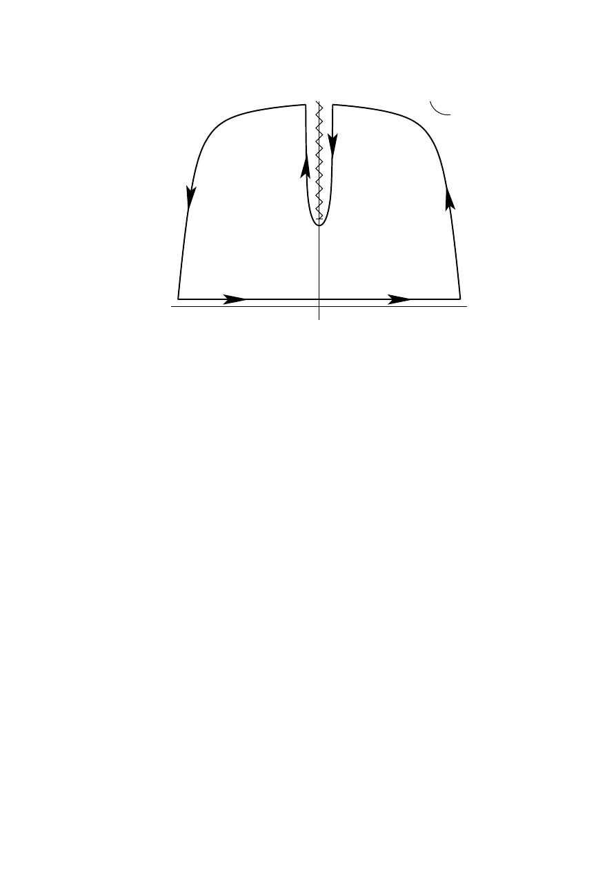
Fig. 6: Illustration of the Casimir effect. In regions I and II the spetrum of modes of the momentum p
⊥
is
continuous, while in the space between the plates (region II) it is quantized in units of
π
d
.
3.2
The Casimir effect
The presence of a vacuum energy is not characteristic of the scalar field. It is also present in other
cases, in particular in quantum electrodynamics. Although one might be tempted to discarding this
infinite contribution to the energy of the vacuum as unphysical, it has observable consequences. In
1948 Hendrik Casimir pointed out [15] that although a formally divergent vacuum energy would
not be observable, any variation in this energy would be (see [16] for comprehensive reviews).
To show this he devised the following experiment. Consider a couple of infinite, perfectly
conducting plates placed parallel to each other at a distance
d (see Fig. 6). Because the conducting
plates fix the boundary condition of the vacuum modes of the electromagnetic field these are discrete
in between the plates (region II), while outside there is a continuous spectrum of modes (regions
I and III). In order to calculate the force between the plates we can take the vacuum energy of
the electromagnetic field as given by the contribution of two scalar fields corresponding to the two
polarizations of the photon. Therefore we can use the formulas derived above.
A naive calculation of the vacuum energy in this system gives a divergent result. This infinity
can be removed, however, by substracting the vacuum energy corresponding to the situation where
the plates are removed
E(d)
reg
= E(d)
vac
− E(∞)
vac
(3.59)
This substraction cancels the contribution of the modes outside the plates. Because of the bound-
ary conditions imposed by the plates the momentum of the modes perpendicular to the plates are
19

quantized according to
p
⊥
=
nπ
d
, with
n a non-negative integer. If we consider that the size of the
plates is much larger than their separation
d we can take the momenta parallel to the plates ~p
k
as
continuous. For
n > 0 we have two polarizations for each vacuum mode of the electromagnetic
field, each contributing like
1
2
q
~p
2
k
+ p
2
⊥
to the vacuum energy. On the other hand, when
p
⊥
= 0 the
corresponding modes of the field are effectively (2+1)-dimensional and therefore there is only one
polarization. Keeping this in mind, we can write
E(d)
reg
= S
Z
d
2
p
k
(2π)
2
1
2
|~p
k
| + 2S
Z
d
2
p
k
(2π)
2
∞
X
n
=1
1
2
r
~p
2
k
+
nπ
d
2
− 2Sd
Z
d
3
p
(2π)
3
1
2
|~p |
(3.60)
where
S is the area of the plates. The factors of 2 take into account the two propagating degrees
of freedom of the electromagnetic field, as discussed above. In order to ensure the convergence of
integrals and infinite sums we can introduce an exponential damping factor
4
E(d)
reg
=
1
2
S
Z
d
2
p
⊥
(2π)
2
e
−
1
Λ
|~p
k
|
|~p
k
| + S
∞
X
n
=1
Z
d
2
p
k
(2π)
2
e
−
1
Λ
r
~
p
2
k
+
(
nπ
d
)
2
r
~p
2
k
+
nπ
d
2
− Sd
Z
∞
−∞
dp
⊥
2π
Z
d
2
p
k
(2π)
2
e
−
1
Λ
q
~
p
2
k
+p
2
⊥
q
~p
2
k
+ p
2
⊥
(3.61)
where
Λ is an ultraviolet cutoff. It is now straightforward to see that if we define the function
F (x) =
1
2π
Z
∞
0
y dy e
−
1
Λ
q
y
2
+
(
xπ
d
)
2
r
y
2
+
xπ
d
2
=
1
4π
Z
∞
(
xπ
d
)
2
dz e
−
√
z
Λ
√
z
(3.62)
the regularized vacuum energy can be written as
E(d)
reg
= S
"
1
2
F (0) +
∞
X
n
=1
F (n)
−
Z
∞
0
dx F (x)
#
(3.63)
This expression can be evaluated using the Euler-MacLaurin formula [18]
∞
X
n
=1
F (n)
−
Z
∞
0
dx F (x) =
−
1
2
[F (0) + F (
∞)] +
1
12
[F
′
(
∞) − F
′
(0)]
−
1
720
[F
′′′
(
∞) − F
′′′
(0)] + . . .
(3.64)
Since for our function
F (
∞) = F
′
(
∞) = F
′′′
(
∞) = 0 and F
′
(0) = 0, the value of E(d)
reg
is
determined by
F
′′′
(0). Computing this term and removing the ultraviolet cutoff, Λ
→ ∞ we find
the result
E(d)
reg
=
S
720
F
′′′
(0) =
−
π
2
S
720d
3
.
(3.65)
4
Actually, one could introduce any cutoff function f
(p
2
⊥
+ p
2
k
) going to zero fast enough as p
⊥
, p
k
→ ∞. The result
is independent of the particular function used in the calculation.
20

Then, the force per unit area between the plates is given by
P
Casimir
=
−
π
2
240
1
d
4
.
(3.66)
The minus sign shows that the force between the plates is attractive. This is the so-called Casimir
effect. It was experimentally measured in 1958 by Sparnaay [17] and since then the Casimir effect
has been checked with better and better precission in a variety of situations [16].
4
Theories and Lagrangians
Up to this point we have used a scalar field to illustrate our discussion of the quantization procedure.
However, nature is richer than that and it is necessary to consider other fields with more complicated
behavior under Lorentz transformations. Before considering other fields we pause and study the
properties of the Lorentz group.
4.1
Representations of the Lorentz group
In four dimensions the Lorentz group has six generators. Three of them correspond to the generators
of the group of rotations in three dimensions SO(3). In terms of the generators
J
i
of the group a
finite rotation of angle
ϕ with respect to an axis determined by a unitary vector ~e can be written as
R(~e, ϕ) = e
−iϕ ~e· ~
J
,
~
J =
J
1
J
2
J
3
.
(4.1)
The other three generators of the Lorentz group are associated with boosts
M
i
along the three spatial
directions. A boost with rapidity
λ along a direction ~u is given by
B(~u, λ) = e
−iλ ~u· ~
M
,
~
M =
M
1
M
2
M
3
.
(4.2)
These six generators satisfy the algebra
[J
i
, J
j
] = iǫ
ijk
J
k
,
[J
i
, M
k
] = iǫ
ijk
M
k
,
(4.3)
[M
i
, M
j
] =
−iǫ
ijk
J
k
,
The first line corresponds to the commutation relations of SO(3), while the second one implies that
the generators of the boosts transform like a vector under rotations.
At first sight, to find representations of the algebra (4.3) might seem difficult. The problem is
greatly simplified if we consider the following combination of the generators
J
±
k
=
1
2
(J
k
± iM
k
).
(4.4)
21
Representation
Type of field
(0, 0)
Scalar
(
1
2
, 0)
Right-handed spinor
(0,
1
2
)
Left-handed spinor
(
1
2
,
1
2
)
Vector
(1, 0)
Selfdual antisymmetric 2-tensor
(0, 1)
Anti-selfdual antisymmetric 2-tensor
Table 1: Representations of the Lorentz group
Using (4.3) it is easy to prove that the new generators
J
±
k
satisfy the algebra
[J
±
i
, J
±
j
] = iǫ
ijk
J
±
k
,
[J
+
i
, J
−
j
] = 0.
(4.5)
Then the Lorentz algebra (4.3) is actually equivalent to two copies of the algebra of
SU(2)
≈ SO(3).
Therefore the irreducible representations of the Lorentz group can be obtained from the well-known
representations of SU(2). Since the latter ones are labelled by the spin s
= k +
1
2
, k (with k
∈ N),
any representation of the Lorentz algebra can be identified by specifying
(s
+
, s
−
), the spins of the
representations of the two copies of SU(2) that made up the algebra (4.3).
To get familiar with this way of labelling the representations of the Lorentz group we study
some particular examples. Let us start with the simplest one
(s
+
, s
−
) = (0, 0). This state is a singlet
under
J
±
i
and therefore also under rotations and boosts. Therefore we have a scalar.
The next interesting cases are
(
1
2
, 0) and (0,
1
2
). They correspond respectively to a right-
handed and a left-handed Weyl spinor. Their properties will be studied in more detail below. In
the case of
(
1
2
,
1
2
), since from Eq. (4.4) we see that J
i
= J
+
i
+ J
−
i
the rules of addition of angular
momentum tell us that there are two states, one of them transforming as a vector and another one as
a scalar under three-dimensional rotations. Actually, a more detailed analysis shows that the singlet
state corresponds to the time component of a vector and the states combine to form a vector under
the Lorentz group.
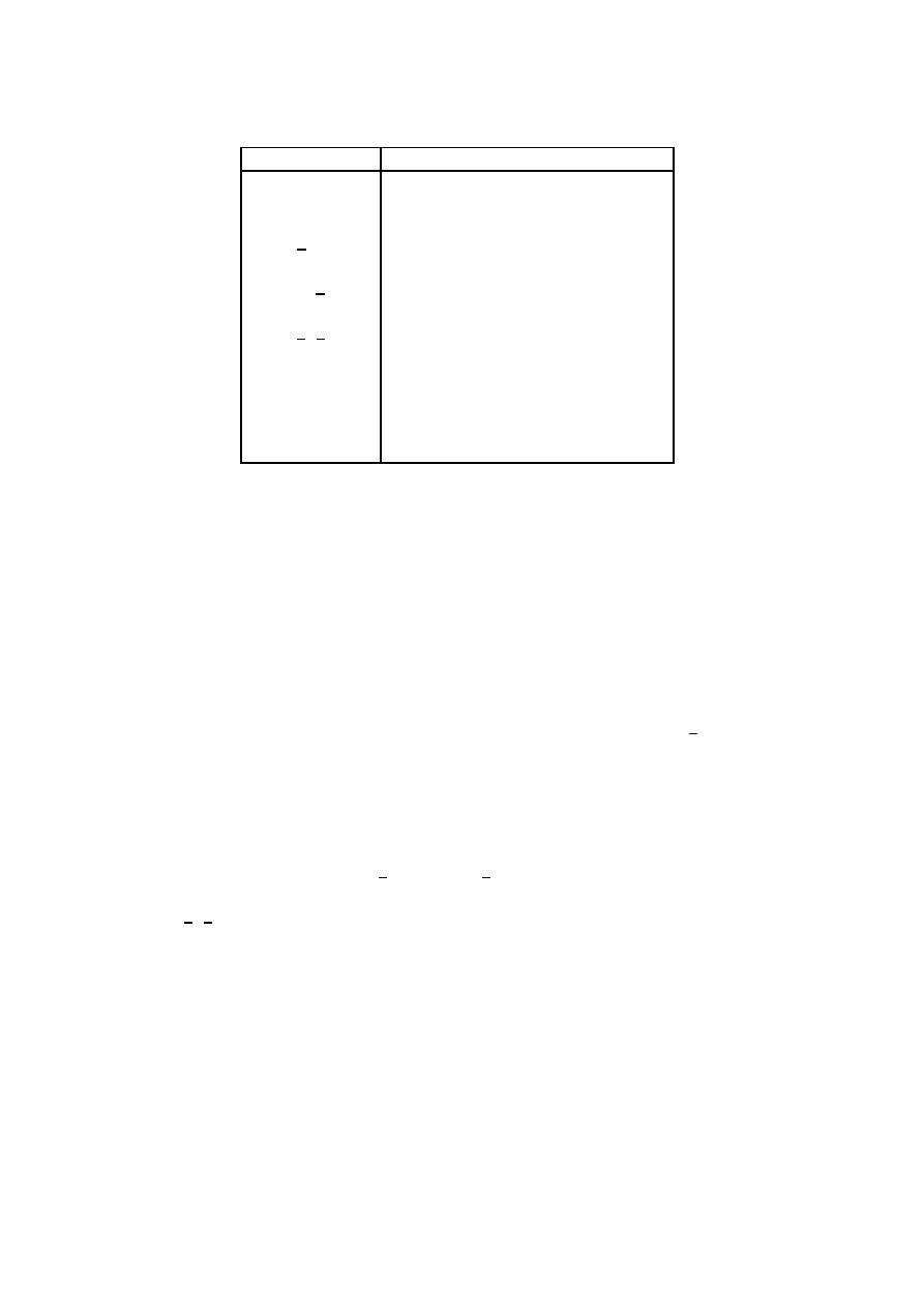
There are also more “exotic” representations. For example we can consider the
(1, 0) and
(0, 1) representations corresponding respectively to a selfdual and an anti-selfdual rank-two anti-
symmetric tensor. In Table 1 we summarize the previous discussion.
To conclude our discussion of the representations of the Lorentz group we notice that under a
22
parity transformation the generators of SO(1,3) transform as
P : J
i
−→ J
i
,
P : M
i
−→ −M
i
(4.6)
this means that
P : J
±
i
−→ J
∓
i
and therefore a representation
(s
1
, s
2
) is transformed into (s
2
, s
1
).
This means that, for example, a vector
(
1
2
,
1
2
) is invariant under parity, whereas a left-handed Weyl
spinor
(
1
2
, 0) transforms into a right-handed one (0,
1
2
) and vice versa.
4.2
Spinors
Weyl spinors. Let us go back to the two spinor representations of the Lorentz group, namely
(
1
2
, 0)
and
(0,
1
2
). These representations can be explicitly constructed using the Pauli matrices as
J
+
i
=
1
2
σ
i
,
J
−
i
= 0
for
(
1
2
, 0),
J
+
i
= 0,
J
−
i
=
1
2
σ
i
for
(0,
1
2
).
(4.7)
We denote by
u
±
a complex two-component object that transforms in the representation s
±
=
1
2
of
J
i
±
. If we define
σ
µ
±
= (1,
±σ
i
) we can construct the following vector quantities
u
†
+
σ
µ
+
u
+
,
u
†
−
σ
µ
−
u
−
.
(4.8)
Notice that since
(J
±
i
)
†
= J
∓
i
the hermitian conjugated fields
u
†
±
are in the
(0,
1
2
) and (
1
2
, 0) respec-
tively.
To construct a free Lagrangian for the fields
u
±
we have to look for quadratic combinations
of the fields that are Lorentz scalars. If we also demand invariance under global phase rotations
u
±
−→ e
iθ
u
±
(4.9)
we are left with just one possibility up to a sign
L
±
Weyl
= iu
†
±
∂
t
± ~σ · ~
∇
u
±
= iu
†
±
σ
µ
±
∂
µ
u
±
.
(4.10)
This is the Weyl Lagrangian. In order to grasp the physical meaning of the spinors
u
±
we write the
equations of motion
∂
0
± ~σ · ~∇
u
±
= 0.
(4.11)
Multiplying this equation on the left by
∂
0
∓ ~σ · ~∇
and applying the algebraic properties of the
Pauli matrices we conclude that
u
±
satisfies the massless Klein-Gordon equation
∂
µ
∂
µ
u
±
= 0,
(4.12)
whose solutions are:
u
±
(x) = u
±
(k)e
−ik·x
,
with
k
0
=
|~k|.
(4.13)
23
Plugging these solutions back into the equations of motion (4.11) we find
|~k| ∓ ~k · ~σ
u
±
= 0,
(4.14)
which implies
u
+
:
~σ
· ~k
|~k|
= 1,
u
−
:
~σ
· ~k
|~k|
=
−1.
(4.15)
Since the spin operator is defined as
~s =
1
2
~σ, the previous expressions give the chirality of the states
with wave function
u
±
, i.e. the projection of spin along the momentum of the particle. Therefore
we conclude that
u
+
is a Weyl spinor of positive helicity
λ =
1
2
, while
u
−
has negative helicity
λ =
−
1
2
. This agrees with our assertion that the representation
(
1
2
, 0) corresponds to a right-handed
Weyl fermion (positive chirality) whereas
(0,
1
2
) is a left-handed Weyl fermion (negative chirality).
For example, in the Standard Model neutrinos are left-handed Weyl spinors and therefore transform
in the representation
(0,
1
2
) of the Lorentz group.
Nevertheless, it is possible that we were too restrictive in constructing the Weyl Lagrangian
(4.10). There we constructed the invariants from the vector bilinears (4.8) corresponding to the
product representations
(
1
2
,
1
2
) = (
1
2
, 0)
⊗ (0,
1
2
)
and
(
1
2
,
1
2
) = (0,
1
2
)
⊗ (
1
2
, 0).
(4.16)
In particular our insistence in demanding the Lagrangian to be invariant under the global symmetry
u
±
→ e
iθ
u
±
rules out the scalar term that appears in the product representations
(
1
2
, 0)
⊗ (
1
2
, 0) = (1, 0)
⊕ (0, 0),
(0,
1
2
)
⊗ (0,
1
2
) = (0, 1)
⊕ (0, 0).
(4.17)
The singlet representations corresponds to the antisymmetric combinations
ǫ
ab
u
a
±
u
b
±
,
(4.18)
where
ǫ
ab
is the antisymmetric symbol
ǫ
12
=
−ǫ
21
= 1.
At first sight it might seem that the term (4.18) vanishes identically because of the antisym-
metry of the
ǫ-symbol. However we should keep in mind that the spin-statistic theorem (more on
this later) demands that fields with half-integer spin have to satisfy the Fermi-Dirac statistics and
therefore satisfy anticommutation relations, whereas fields of integer spin follow the statistic of
Bose-Einstein and, as a consequence, quantization replaces Poisson brackets by commutators. This
implies that the components of the Weyl fermions
u
±
are anticommuting Grassmann fields
u
a
±
u
b
±
+ u
b
±
u
a
±
= 0.
(4.19)
It is important to realize that, strictly speaking, fermions (i.e., objects that satisfy the Fermi-Dirac
statistics) do not exist classically. The reason is that they satisfy the Pauli exclusion principle and
24

therefore each quantum state can be occupied, at most, by one fermion. Therefore the na¨ıve defini-
tion of the classical limit as a limit of large occupation numbers cannot be applied. Fermion field
do not really make sense classically.
Since the combination (4.18) does not vanish and we can construct a new Lagrangian
L
±
Weyl
= iu
†
±
σ
µ
±
∂
µ
u
±
+
1
2
mǫ
ab
u
a
±
u
b
±
+ h.c.
(4.20)
This mass term, called of Majorana type, is allowed if we do not worry about breaking the global
U(1) symmetry
u
±
→ e
iθ
u
±
. This is not the case, for example, of charged chiral fermions, since the
Majorana mass violates the conservation of electric charge or any other gauge U(1) charge. In the
Standard Model, however, there is no such a problem if we introduce Majorana masses for right-
handed neutrinos, since they are singlet under all standard model gauge groups. Such a term will
break, however, the global U(1) lepton number charge because the operator
ǫ
ab
ν
a
R
ν
b
R
changes the
lepton number by two units
Dirac spinors. We have seen that parity interchanges the representations
(
1
2
, 0) and (0,
1
2
),
i.e. it changes right-handed with left-handed fermions
P : u
±
−→ u
∓
.
(4.21)
An obvious way to build a parity invariant theory is to introduce a pair or Weyl fermions
u
+
and
u
+
.
Actually, these two fields can be combined in a single four-component spinor
ψ =
u
+
u
−
(4.22)
transforming in the reducible representation
(
1
2
, 0)
⊕ (0,
1
2
).
Since now we have both
u
+
and
u
−
simultaneously at our disposal the equations of motion
for
u
±
,
iσ
µ
±
∂
µ
u
±
= 0 can be modified, while keeping them linear, to
iσ
µ
+
∂
µ
u
+
= mu
−
iσ
µ
−
∂
µ
u
−
= mu
+
=
⇒
i
σ
µ
+
0
0
σ
µ
−
∂
µ
ψ = m
0 1
1
0
ψ.
(4.23)
These equations of motion can be derived from the Lagrangian density
L
Dirac
= iψ
†
σ
µ
+
0
0
σ
µ
−
∂
µ
ψ
− mψ
†
0 1
1
0
ψ.
(4.24)
To simplify the notation it is useful to define the Dirac
γ-matrices as
γ
µ
=
0
σ
µ
−
σ
µ
+
0
(4.25)
and the Dirac conjugate spinor
ψ
ψ
≡ ψ
†
γ
0
= ψ
†
0 1
1
0
.
(4.26)
25

Now the Lagrangian (4.24) can be written in the more compact form
L
Dirac
= ψ (iγ
µ
∂
µ
− m) ψ.
(4.27)
The associated equations of motion give the Dirac equation (2.9) with the identifications
γ
0
= β,
γ
i
= iα
i
.
(4.28)
In addition, the
γ-matrices defined in (4.25) satisfy the Clifford algebra
{γ
µ
, γ
ν
} = 2η
µν
.
(4.29)
In
D dimensions this algebra admits representations of dimension 2
[
D
2
]
. When
D is even the Dirac
fermions
ψ transform in a reducible representation of the Lorentz group. In the case of interest,
D = 4 this is easy to prove by defining the matrix
γ
5
=
−iγ
0
γ
1
γ
2
γ
3
=
1
0
0
−1
.
(4.30)
We see that
γ
5
anticommutes with all other
γ-matrices. This implies that
[γ
5
, σ
µν
] = 0,
with
σ
µν
=
−
i
4
[γ
µ
, γ
ν
].
(4.31)
Because of Schur’s lemma (see Appendix) this implies that the representation of the Lorentz group
provided by
σ
µν
is reducible into subspaces spanned by the eigenvectors of
γ
5
with the same eigen-
value. If we define the projectors
P
±
=
1
2
(1
± γ
5
) these subspaces correspond to
P
+
ψ =
u
+
0
,
P
−
ψ =
0
u
−
,
(4.32)
which are precisely the Weyl spinors introduced before.
Our next task is to quantize the Dirac Lagrangian. This will be done along the lines used for
the Klein-Gordon field, starting with a general solution to the Dirac equation and introducing the
corresponding set of creation-annihilation operators. Therefore we start by looking for a complete
basis of solutions to the Dirac equation. In the case of the scalar field the elements of the basis were
labelled by their four-momentum
k
µ
. Now, however, we have more degrees of freedom since we
are dealing with a spinor which means that we have to add extra labels. Looking back at Eq. (4.15)
we can define the helicity operator for a Dirac spinor as
λ =
1
2
~σ
·
~k
|~k|
1
0
0 1
.
(4.33)
Hence, each element of the basis of functions is labelled by its four-momentum
k
µ
and the corre-
sponding eigenvalue
s of the helicity operator. For positive energy solutions we then propose the
ansatz
u(k, s)e
−ik·x
,
s =
±
1
2
,
(4.34)
26
where
u
α
(k, s) (α = 1, . . . , 4) is a four-component spinor. Substituting in the Dirac equation we
obtain
(/k
− m)u(k, s) = 0.
(4.35)
In the same way, for negative energy solutions we have
v(k, s)e
ik
·x
,
s =
±
1
2
,
(4.36)
where
v(k, s) has to satisfy
(/k + m)v(k, s) = 0.
(4.37)
Multiplying Eqs. (4.35) and (4.37) on the left respectively by
(/k
∓ m) we find that the momentum
is on the mass shell,
k
2
= m
2
. Because of this, the wave function for both positive- and negative-
energy solutions can be labeled as well using the three-momentum ~
k of the particle, u(~k, s), v(~k, s).
A detailed analysis shows that the functions
u(~k, s), v(~k, s) satisfy the properties
u(~k, s)u(~k, s) = 2m,
v(~k, s)v(~k, s) =
−2m,
u(~k, s)γ
µ
u(~k, s) = 2k
µ
,
v(~k, s)γ
µ
v(~k, s) = 2k
µ
,
(4.38)
X
s
=±
1
2
u
α
(~k, s)u
β
(~k, s) = (/k + m)
αβ
,
X
s
=±
1
2
v
α
(~k, s)v
β
(~k, s) = (/k
− m)
αβ
,
with
k
0
= ω
k
=
p
~k
2
+ m
2
. Then, a general solution to the Dirac equation including creation and
annihilation operators can be written as:
b
ψ(t, ~x) =
Z
d
3
k
(2π)
3
1
2ω
k
X
s
=±
1
2
h
u(~k, s) bb(~k, s)e
−iω
k
t
+i~k·~x
+ v(~k, s) b
d
†
(~k, s)e
iω
k
t
−i~k·~x
i
.
(4.39)
The operators b
b
†
α
(~k, s), bb
α
(~k) respectively create and annihilate a spin-
1
2
particle (for example,
an electron) out of the vacuum with momentum ~
k and helicity s. Because we are dealing with
half-integer spin fields, the spin-statistics theorem forces canonical anticommutation relations for b
ψ
which means that the creation-annihilation operators satisfy the algebra
5
{b
α
(~k, s), b
†
β
(~k
′
, s
′
)
} = δ(~k − ~k
′
)δ
αβ
δ
ss
′
,
{b
α
(~k, s), b
β
(~k
′
, s
′
)
} = {b
†
α
(~k, s), b
†
β
(~k
′
, s
′
)
} = 0.
(4.40)
In the case of
d
a
(~k, s), d
†
a
(~k, s) we have a set of creation-annihilation operators for the corre-
sponding antiparticles (for example positrons). This is clear if we notice that
d
†
a
(~k, s) can be seen
as the annihilation operator of a negative energy state of the Dirac equation with wave function
5
To simplify notation, and since there is no risk of confusion, we drop from now on the hat to indicate operators.
27

v
a
(~k, s). As we saw, in the Dirac sea picture this corresponds to the creation of an antiparticle out
of the vacuum (see Fig. 2). The creation-annihilation operators for antiparticles also satisfy the
fermionic algebra
{d
α
(~k, s), d
†
β
(~k
′
, s
′
)
} = δ(~k − ~k
′
)δ
αβ
δ
ss
′
,
{d
α
(~k, s), d
β
(~k
′
, s
′
)
} = {d
†
α
(~k, s), d
†
β
(~k
′
, s
′
)
} = 0.
(4.41)
All other anticommutators between
b
α
(~k, s), b
†
α
(~k, s) and d
α
(~k, s), d
†
α
(~k, s) vanish.
The Hamiltonian operator for the Dirac field is
b
H =
X
s
=±
1
2
Z
d
3
k
h
ω
k
b
†
α
(~k, s)b
α
(~k, s)
− ω
k
d
α
(~k, s)d
†
α
(~k, s)
i
.
(4.42)
At this point we realize again of the necessity of quantizing the theory using anticommutators in-
stead of commutators. Had we use canonical commutation relations, the second term inside the
integral in (4.42) would give the number operator
d
†
α
(~k, s)d
α
(~k, s) with a minus sign in front. As a
consequence the Hamiltonian would be unbounded from below and we would be facing again the
instability of the theory already noticed in the context of relativistic quantum mechanics. However,
because of the anticommutation relations (4.41), the Hamiltonian (4.42) takes the form
b
H =
X
s
=±
1
2
Z
d
3
k
h
ω
k
b
†
α
(~k, s)b
α
(~k, s) + ω
k
d
†
α
(~k, s)d
α
(~k, s)
− ω
k
δ(~0)
i
.
(4.43)
As with the scalar field, we find a divergent vacuum energy contribution due to the zero-point energy
of the infinite number of harmonic oscillators. Unlike the Klein-Gordon field, the vacuum energy
is negative. In section 9.2 we will see that in certain type of theories called supersymmetric, where
the number of bosonic and fermionic degrees of freedom is the same, there is a cancellation of the
vacuum energy. The divergent contribution can be removed by the normal order prescription
: b
H:=
X
s
=±
1
2
Z
d
3
k
h
ω
k
b
†
α
(~k, s)b
α
(~k, s) + ω
k
d
†
α
(~k, s)d
α
(~k, s)
i
.
(4.44)
Finally, let us mention that using the Dirac equation it is easy to prove that there is a conserved
four-current given by
j
µ
= ψγ
µ
ψ,
∂
µ
j
µ
= 0.
(4.45)
As we will explain further in sec. 6 this current is associated to the invariance of the Dirac La-
grangian under the global phase shift
ψ
→ e
iθ
ψ. In electrodynamics the associated conserved
charge
Q = e
Z
d
3
x j
0
(4.46)
is identified with the electric charge.
28

4.3
Gauge fields
In classical electrodynamics the basic quantities are the electric and magnetic fields ~
E, ~
B. These
can be expressed in terms of the scalar and vector potential
(ϕ, ~
A)
~
E =
−~∇ϕ −
∂ ~
A
∂t
,
~
B = ~
∇ × ~
A.
(4.47)
From these equations it follows that there is an ambiguity in the definition of the potentials given by
the gauge transformations
ϕ(t, ~x)
→ ϕ(t, ~x) +
∂
∂t
ǫ(t, ~x),
~
A(t, ~x)
→ ~
A(t, ~x) + ~
∇ǫ(t, ~x).
(4.48)
Classically
(ϕ, ~
A) are seen as only a convenient way to solve the Maxwell equations, but without
physical relevance.
The equations of electrodynamics can be recast in a manifestly Lorentz invariant form using
the four-vector gauge potential
A
µ
= (ϕ, ~
A) and the antisymmetric rank-two tensor: F
µν
= ∂
µ
A
ν
−
∂
ν
A
µ
. Maxwell’s equations become
∂
µ
F
µν
= j
µ
,
ǫ
µνση
∂
ν
F
ση
= 0,
(4.49)
where the four-current
j
µ
= (ρ, ~) contains the charge density and the electric current. The field
strength tensor
F
µν
and the Maxwell equations are invariant under gauge transformations (4.48),
which in covariant form read
A
µ
−→ A
µ
+ ∂
µ
ǫ.
(4.50)
Finally, the equations of motion of charged particles are given, in covariant form, by
m
du
µ
dτ
= eF
µν
u
ν
,
(4.51)
where
e is the charge of the particle and u
µ
(τ ) its four-velocity as a function of the proper time.
The physical rˆole of the vector potential becomes manifest only in Quantum Mechanics. Us-
ing the prescription of minimal substitution
~p
→ ~p − e ~
A, the Schr¨odinger equation describing a
particle with charge
e moving in an electromagnetic field is
i∂
t
Ψ =
−
1
2m
~
∇ − ie ~
A
2
+ eϕ
Ψ.
(4.52)
Because of the explicit dependence on the electromagnetic potentials
ϕ and ~
A, this equation seems
to change under the gauge transformations (4.48). This is physically acceptable only if the ambi-
guity does not affect the probability density given by
|Ψ(t, ~x)|
2
. Therefore, a gauge transformation
29

of the electromagnetic potential should amount to a change in the (unobservable) phase of the wave
function. This is indeed what happens: the Schr¨odinger equation (4.52) is invariant under the gauge
transformations (4.48) provided the phase of the wave function is transformed at the same time
according to
Ψ(t, ~x)
−→ e
−ie ǫ(t,~x)
Ψ(t, ~x).
(4.53)
Aharonov-Bohm effect. This interplay between gauge transformations and the phase of the
wave function give rise to surprising phenomena. The first evidence of the rˆole played by the
electromagnetic potentials at the quantum level was pointed out by Yakir Aharonov and David
Bohm [19]. Let us consider a double slit experiment as shown in Fig. 7, where we have placed a
shielded solenoid just behind the first screen. Although the magnetic field is confined to the interior
of the solenoid, the vector potential is nonvanishing also outside. Of course the value of ~
A outside
the solenoid is a pure gauge, i.e. ~
∇ × ~
A = ~0, however because the region outside the solenoid is not
simply connected the vector potential cannot be gauged to zero everywhere. If we denote by
Ψ
(0)
1
and
Ψ
(0)
2
the wave functions for each of the two electron beams in the absence of the solenoid, the
total wave function once the magnetic field is switched on can be written as
Ψ = e
ie
R
Γ1
~
A
·d~x
Ψ
(0)
1
+ e
ie
R
Γ2
~
A
·d~x
Ψ
(0)
2
= e
ie
R
Γ1
~
A
·d~x
h
Ψ
(0)
1
+ e
ie
H
Γ
~
A
·d~x
Ψ
(0)
2
i
,
(4.54)
where
Γ
1
and
Γ
2
are two curves surrounding the solenoid from different sides, and
Γ is any closed
loop surrounding it. Therefore the relative phase between the two beams gets an extra term depend-
ing on the value of the vector potential outside the solenoid as
U = exp
ie
I
Γ
~
A
· d~x
.
(4.55)
Because of the change in the relative phase of the electron wave functions, the presence of the
vector potential becomes observable even if the electrons do not feel the magnetic field. If we
perform the double-slit experiment when the magnetic field inside the solenoid is switched off we
will observe the usual interference pattern on the second screen. However if now the magnetic field
is switched on, because of the phase (4.54), a change in the interference pattern will appear. This is
the Aharonov-Bohm effect.
The first question that comes up is what happens with gauge invariance. Since we said that
~
A can be changed by a gauge transformation it seems that the resulting interference patters might
depend on the gauge used. Actually, the phase
U in (4.55) is independent of the gauge although,
unlike other gauge-invariant quantities like ~
E and ~
B, is nonlocal. Notice that, since ~
∇ × ~
A = ~0
outside the solenoid, the value of
U does not change under continuous deformations of the closed
curve
Γ, so long as it does not cross the solenoid.
The Dirac monopole. It is very easy to check that the vacuum Maxwell equations remain
invariant under the transformation
~
E
− i ~
B
−→ e
iθ
( ~
E
− i ~
B),
θ
∈ [0, 2π]
(4.56)
30
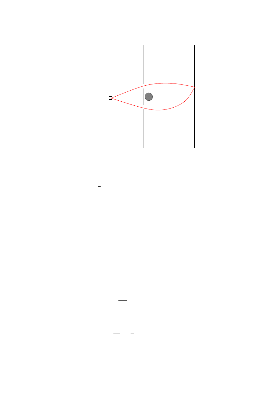
Γ
1
Γ
2
Screen
Electron
S
source
Fig. 7: Illustration of an interference experiment to show the Aharonov-Bohm effect. S represent the solenoid
in whose interior the magnetic field is confined.
which, in particular, for
θ =
π
2
interchanges the electric and the magnetic fields: ~
E
→ ~
B, ~
B
→ − ~
E.
This duality symmetry is however broken in the presence of electric sources. Nevertheless the
Maxwell equations can be “completed” by introducing sources for the magnetic field
(ρ
m
, ~
m
) in
such a way that the duality (4.56) is restored when supplemented by the transformation
ρ
− iρ
m
−→ e
iθ
(ρ
− iρ
m
),
~
− i~
m
−→ e
iθ
(~
− i~
m
).
(4.57)
Again for
θ = π/2 the electric and magnetic sources get interchanged.
In 1931 Dirac [20] studied the possibility of finding solutions of the completed Maxwell
equation with a magnetic monopoles of charge
g, i.e. solutions to
~
∇ · ~
B = g δ(~x).
(4.58)
Away from the position of the monopole ~
∇ · ~
B = 0 and the magnetic field can be still derived
locally from a vector potential ~
A according to ~
B = ~
∇ × ~
A. However, the vector potential cannot
be regular everywhere since otherwise Gauss law would imply that the magnetic flux threading a
closed surface around the monopole should vanish, contradicting (4.58).
We look now for solutions to Eq. (4.58). Working in spherical coordinates we find
B
r
=
g
|~x|
2
,
B
ϕ
= B
θ
= 0.
(4.59)
Away from the position of the monopole (
~x
6= ~0) the magnetic field can be derived from the vector
potential
A
ϕ
=
g
|~x|
tan
θ
2
,
A
r
= A
θ
= 0.
(4.60)
31
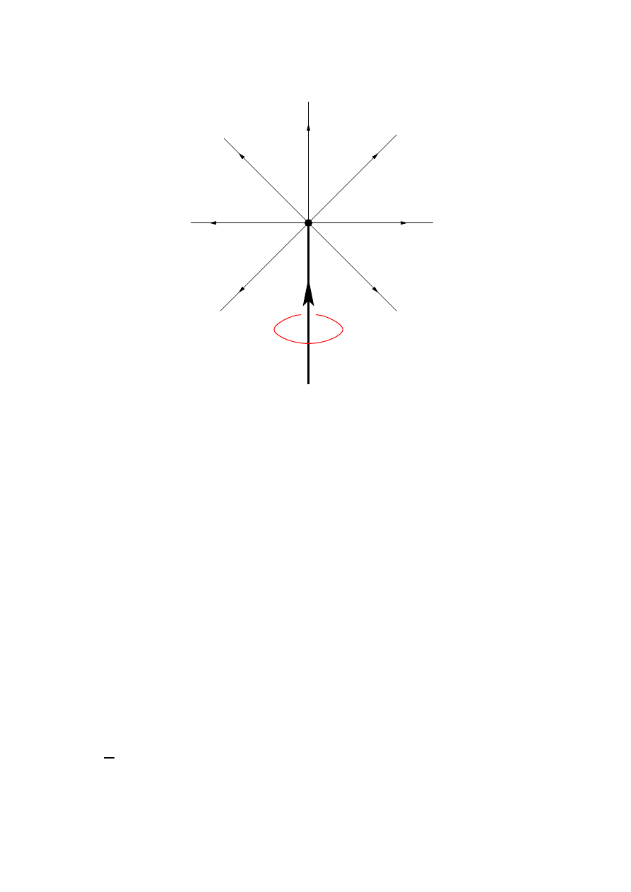
Dirac string
Γ
g
Fig. 8: The Dirac monopole.
As expected we find that this vector potential is actually singular around the half-line
θ = π (see
Fig. 8). This singular line starting at the position of the monopole is called the Dirac string and
its position changes with a change of gauge but cannot be eliminated by any gauge transformation.
Physically we can see it as an infinitely thin solenoid confining a magnetic flux entering into the
magnetic monopole from infinity that equals the outgoing magnetic flux from the monopole.
Since the position of the Dirac string depends on the gauge chosen it seems that the presence
of monopoles introduces an ambiguity. This would be rather strange, since Maxwell equations
are gauge invariant also in the presence of magnetic sources. The solution to this apparent riddle
lies in the fact that the Dirac string does not pose any consistency problem as far as it does not
produce any physical effect, i.e. if its presence turns out to be undetectable. From our discussion
of the Aharonov-Bohm effect we know that the wave function of charged particles pick up a phase
(4.55) when surrounding a region where magnetic flux is confined (for example the solenoid in the
Aharonov-Bohm experiment). As explained above, the Dirac string associated with the monopole
can be seen as a infinitely thin solenoid. Therefore the Dirac string will be unobservable if the phase
picked up by the wave function of a charged particle is equal to one. A simple calculation shows
that this happens if
e
i e g
= 1
=
⇒
e g = 2πn with n
∈ Z.
(4.61)
Interestingly, this discussion leads to the conclusion that the presence of a single magnetic mono-
poles somewhere in the Universe implies for consistency the quantization of the electric charge in
units of
2π
g
, where
g the magnetic charge of the monopole.
32
Quantization of the electromagnetic field. We now proceed to the quantization of the elec-
tromagnetic field in the absence of sources
ρ = 0, ~ = ~0. In this case the Maxwell equations (4.49)
can be derived from the Lagrangian density
L
Maxwell
=
−
1
4
F
µν
F
µν
=
1
2
~
E
2
− ~
B
2
.
(4.62)
Although in general the procedure to quantize the Maxwell Lagrangian is not very different from
the one used for the Klein-Gordon or the Dirac field, here we need to deal with a new ingredient:
gauge invariance. Unlike the cases studied so far, here the photon field
A
µ
is not unambiguously
defined because the action and the equations of motion are insensitive to the gauge transformations
A
µ
→ A
µ
+ ∂
µ
ε. A first consequence of this symmetry is that the theory has less physical degrees
of freedom than one would expect from the fact that we are dealing with a vector field.
The way to tackle the problem of gauge invariance is to fix the freedom in choosing the
electromagnetic potential before quantization. This can be done in several ways, for example by
imposing the Lorentz gauge fixing condition
∂
µ
A
µ
= 0.
(4.63)
Notice that this condition does not fix completely the gauge freedom since Eq. (4.63) is left invariant
by gauge transformations satisfying
∂
µ
∂
µ
ε = 0. One of the advantages, however, of the Lorentz
gauge is that it is covariant and therefore does not pose any danger to the Lorentz invariance of the
quantum theory. Besides, applying it to the Maxwell equation
∂
µ
F
µν
= 0 one finds
0 = ∂
µ
∂
µ
A
ν
− ∂
ν
(∂
µ
A
µ
) = ∂
µ
∂
µ
A
ν
,
(4.64)
which means that since
A
µ
satisfies the massless Klein-Gordon equation the photon, the quantum
of the electromagnetic field, has zero mass.
Once gauge invariance is fixed
A
µ
is expanded in a complete basis of solutions to (4.64) and
the canonical commutation relations are imposed
b
A
µ
(t, ~x) =
X
λ
=±1
Z
d
3
k
(2π)
3
1
2
|~k|
h
ǫ
µ
(~k, λ)ba(~k, λ)e
−i|~k|t+i~k·~x
+ ǫ
µ
(~k, λ)
∗
ba
†
(~k, λ)e
i
|~k|t−i~k·~x
i
(4.65)
where
λ =
±1 represent the helicity of the photon, and ǫ
µ
(~k, λ) are solutions to the equations of
motion with well defined momentum an helicity. Because of (4.63) the polarization vectors have to
be orthogonal to
k
µ
k
µ
ǫ
µ
(~k, λ) = k
µ
ǫ
µ
(~k, λ)
∗
= 0.
(4.66)
The canonical commutation relations imply that
[ba(~k, λ), ba
†
(~k
′
, λ
′
)] = iδ(~k
− ~k
′
)δ
λλ
′
[ba(~k, λ), ba(~k
′
, λ
′
)] = [ba
†
(~k, λ), ba
†
(~k
′
, λ
′
)] = 0.
(4.67)
33
Therefore
ba(~k, λ), ba
†
(~k, λ) form a set of creation-annihilation operators for photons with momentum
~k and helicity λ.
Behind the simple construction presented above there are a number of subleties related with
gauge invariance. In particular the gauge freedom seem to introduce states in the Hilbert space with
negative probability. A careful analysis shows that when gauge invariance if properly handled these
spurious states decouple from physical states and can be eliminated. The details can be found in
standard textbooks [1–10].
Coupling gauge fields to matter. Once we know how to quantize the electromagnetic field
we consider theories containing electrically charged particles, for example electrons. To couple
the Dirac Lagrangian to electromagnetism we use as guiding principle what we learned about the
Schr¨odinger equation for a charged particle. There we saw that the gauge ambiguity of the electro-
magnetic potential is compensated with a U(1) phase shift in the wave function. In the case of the
Dirac equation we know that the Lagrangian is invariant under
ψ
→ e
ieε
ψ, with ε a constant. How-
ever this invariance is broken as soon as one identifies
ε with the gauge transformation parameter of
the electromagnetic field which depends on the position.
Looking at the Dirac Lagrangian (4.27) it is easy to see that in order to promote the global
U(1) symmetry into a local one,
ψ
→ e
ieε
(x)
ψ, it suffices to replace the ordinary derivative ∂
µ
by a
covariant one
D
µ
satisfying
D
µ
e
ieε
(x)
ψ
= e
ieε
(x)
D
µ
ψ.
(4.68)
This covariant derivative can be constructed in terms of the gauge potential
A
µ
as
D
µ
= ∂
µ
− ieA
µ
.
(4.69)
The Lagrangian of a spin-
1
2
field coupled to electromagnetism is written as
L
QED
=
−
1
4
F
µν
F
µν
+ ψ(i/
D
− m)ψ,
(4.70)
invariant under the gauge transformations
ψ
−→ e
ieε
(x)
ψ,
A
µ
−→ A
µ
+ ∂
µ
ε(x).
(4.71)
Unlike the theories we have seen so far, the Lagrangian (4.70) describe an interacting theory.
By plugging (4.69) into the Lagrangian we find that the interaction between fermions and photons
to be
L
(int)
QED
=
−eA
µ
ψγ
µ
ψ.
(4.72)
As advertised above, in the Dirac theory the electric current four-vector is given by
j
µ
= eψγ
µ
ψ.
The quantization of interacting field theories poses new problems that we did not meet in the
case of the free theories. In particular in most cases it is not possible to solve the theory exactly.
When this happens the physical observables have to be computed in perturbation theory in powers
34
of the coupling constant. An added problem appears when computing quantum corrections to the
classical result, since in that case the computation of observables are plagued with infinities that
should be taken care of. We will go back to this problem in section 8.
Nonabelian gauge theories. Quantum electrodynamics (QED) is the simplest example of a
gauge theory coupled to matter based in the abelian gauge symmetry of local U(1) phase rotations.
However, it is possible also to construct gauge theories based on nonabelian groups. Actually, our
knowledge of the strong and weak interactions is based on the use of such nonabelian generalizations
of QED.
Let us consider a gauge group
G with generators T
a
,
a = 1, . . . , dim G satisfying the Lie
algebra
6
[T
a
, T
b
] = if
abc
T
c
.
(4.73)
A gauge field taking values on the Lie algebra of
G can be introduced A
µ
≡ A
a
µ
T
a
which transforms
under a gauge transformations as
A
µ
−→
1
ig
U∂
µ
U
−1
+ UA
µ
U
−1
,
U = e
iχ
a
(x)T
a
,
(4.74)
where
g is the coupling constant. The associated field strength is defined as
F
a
µν
= ∂
µ
A
a
ν
− ∂
ν
A
a
µ
− gf
abc
A
b
µ
A
c
ν
.
(4.75)
Notice that this definition of the
F
a
µν
reduces to the one used in QED in the abelian case when
f
abc
= 0. In general, however, unlike the case of QED the field strength is not gauge invariant. In
terms of
F
µν
= F
a
µν
T
a
it transforms as
F
µν
−→ UF
µν
U
−1
.
(4.76)
The coupling of matter to a nonabelian gauge field is done by introducing again a covariant
derivative. For a field in a representation of
G
Φ
−→ UΦ
(4.77)
the covariant derivative is given by
D
µ
Φ = ∂
µ
Φ
− igA
a
µ
T
a
Φ.
(4.78)
With the help of this we can write a generic Lagrangian for a nonabelian gauge field coupled to
scalars
φ and spinors ψ as
L = −
1
4
F
a
µν
F
µν a
+ iψ/
Dψ + D
µ
φD
µ
φ
− ψ [M
1
(φ) + iγ
5
M
2
(φ)] ψ
− V (φ).
(4.79)
In order to keep the theory renormalizable we have to restrict
M
1
(φ) and M
2
(φ) to be at most linear
in
φ whereas V (φ) have to be at most of quartic order. The Lagrangian of the Standard Model is of
the form (4.79).
6
Some basics facts about Lie groups have been summarized in Appendix A.
35

4.4
Understanding gauge symmetry
In classical mechanics the use of the Hamiltonian formalism starts with the replacement of general-
ized velocities by momenta
p
i
≡
∂L
∂ ˙q
i
=
⇒
˙q
i
= ˙q
i
(q, p).
(4.80)
Most of the times there is no problem in inverting the relations
p
i
= p
i
(q, ˙q). However in some
systems these relations might not be invertible and result in a number of constraints of the type
f
a
(q, p) = 0,
a = 1, . . . , N
1
.
(4.81)
These systems are called degenerate or constrained [22, 23].
The presence of constraints of the type (4.81) makes the formulation of the Hamiltonian for-
malism more involved. The first problem is related to the ambiguity in defining the Hamiltonian,
since the addition of any linear combination of the constraints do not modify its value. Secondly,
one has to make sure that the constraints are consistent with the time evolution in the system. In the
language of Poisson brackets this means that further constraints have to be imposed in the form
{f
a
, H
} ≈ 0.
(4.82)
Following [22] we use the symbol
≈ to indicate a “weak” equality that holds when the constraints
f
a
(q, p) = 0 are satisfied. Notice however that since the computation of the Poisson brackets
involves derivatives, the constraints can be used only after the bracket is computed. In principle
the conditions (4.82) can give rise to a new set of constraints
g
b
(q, p) = 0, b = 1, . . . , N
2
. Again
these constraints have to be consistent with time evolution and we have to repeat the procedure.
Eventually this finishes when a set of constraints is found that do not require any further constraint
to be preserved by the time evolution
7
.
Once we find all the constraints of a degenerate system we consider the so-called first class
constraints
φ
a
(q, p) = 0, a = 1, . . . , M, which are those whose Poisson bracket vanishes weakly
{φ
a
, φ
b
} = c
abc
φ
c
≈ 0.
(4.83)
The constraints that do not satisfy this condition, called second class constraints, can be eliminated
by modifying the Poisson bracket [22]. Then the total Hamiltonian of the theory is defined by
H
T
= p
i
q
i
− L +
M
X
a
=1
λ(t)φ
a
.
(4.84)
What has all this to do with gauge invariance? The interesting answer is that for a singular
system the first class constraints
φ
a
generate gauge transformations. Indeed, because
{φ
a
, φ
b
} ≈
7
In principle it is also possible that the procedure finishes because some kind of inconsistent identity is found. In
this case the system itself is inconsistent as it is the case with the Lagrangian L
(q, ˙q) = q.
36
0
≈ {φ
a
, H
} the transformations
q
i
−→ q
i
+
M
X
a
ε
a
(t)
{q
i
, φ
a
},
p
i
−→ p
i
+
M
X
a
ε
a
(t)
{p
i
, φ
a
}
(4.85)
leave invariant the state of the system. This ambiguity in the description of the system in terms of the
generalized coordinates and momenta can be traced back to the equations of motion in Lagrangian
language. Writing them in the form
∂
2
L
∂ ˙q
i
∂ ˙q
j
¨
q
j
=
−
∂
2
L
∂ ˙q
i
∂q
j
˙q
j
+
∂L
∂q
i
,
(4.86)
we find that order to determine the accelerations in terms of the positions and velocities the matrix
∂
2
L
∂
˙q
i
∂
˙q
j
has to be invertible. However, the existence of constraints (4.81) precisely implies that the
determinant of this matrix vanishes and therefore the time evolution is not uniquely determined in
terms of the initial conditions.
Let us apply this to Maxwell electrodynamics described by the Lagrangian
L =
−
1
4
Z
d
3
F
µν
F
µν
.
(4.87)
The generalized momentum conjugate to
A
µ
is given by
π
µ
=
δL
δ(∂
0
A
µ
)
= F
0µ
.
(4.88)
In particular for the time component we find the constraint
π
0
= 0. The Hamiltonian is given by
H =
Z
d
3
x [π
µ
∂
0
A
µ
− L] =
Z
d
3
x
1
2
~
E
2
+ ~
B
2
+ π
0
∂
0
A
0
+ A
0
~
∇ · ~
E
.
(4.89)
Requiring the consistency of the constraint
π
0
= 0 we find a second constraint
{π
0
, H
} ≈ ∂
0
π
0
+ ~
∇ · ~
E = 0.
(4.90)
Together with the first constraint
π
0
= 0 this one implies Gauss’ law ~
∇· ~
E = 0. These two constrains
have vanishing Poisson bracket and therefore they are first class. Therefore the total Hamiltonian is
given by
H
T
= H +
Z
d
3
x
h
λ
1
(x)π
0
+ λ
2
(x)~
∇ · ~
E
i
,
(4.91)
where we have absorbed
A
0
in the definition of the arbitrary functions
λ
1
(x) and λ
2
(x). Actually,
we can fix part of the ambiguity taking
λ
1
= 0. Notice that, because A
0
has been included in the
37

multipliers, fixing
λ
1
amounts to fixing the value of
A
0
and therefore it is equivalent to taking a
temporal gauge. In this case the Hamiltonian is
H
T
=
Z
d
3
x
1
2
~
E
2
+ ~
B
2
+ ε(x)~
∇ · ~
E
(4.92)
and we are left just with Gauss’ law as the only constraint. Using the canonical commutation
relations
{A
i
(t, ~x), E
j
(t, ~x
′
)
} = δ
ij
δ(~x
− ~x
′
)
(4.93)
we find that the remaining gauge transformations are generated by Gauss’ law
δA
i
=
{A
i
,
Z
d
3
x
′
ε ~
∇ · ~
E
} = ∂
i
ε,
(4.94)
while leaving
A
0
invariant, so for consistency with the general gauge transformations the function
ε(x) should be independent of time. Notice that the constraint ~
∇ · ~
E = 0 can be implemented by
demanding ~
∇ · ~
A = 0 which reduces the three degrees of freedom of ~
A to the two physical degrees
of freedom of the photon.
So much for the classical analysis. In the quantum theory the constraint ~
∇ · ~
E = 0 has to be
imposed on the physical states
|physi. This is done by defining the following unitary operator on
the Hilbert space
U(ε) ≡ exp
i
Z
d
3
x ε(~x) ~
∇ · ~
E
.
(4.95)
By definition, physical states should not change when a gauge transformations is performed. This
is implemented by requiring that the operator
U(ε) acts trivially on a physical state
U(ε)|physi = |physi
=
⇒
(~
∇ · ~
E)
|physi = 0.
(4.96)
In the presence of charge density
ρ, the condition that physical states are annihilated by Gauss’ law
changes to
(~
∇ · ~
E
− ρ)|physi = 0.
The role of gauge transformations in the quantum theory is very illuminating in understanding
the real rˆole of gauge invariance [24]. As we have learned, the existence of a gauge symmetry in a
theory reflects a degree of redundancy in the description of physical states in terms of the degrees
of freedom appearing in the Lagrangian. In Classical Mechanics, for example, the state of a system
is usually determined by the value of the canonical coordinates
(q
i
, p
i
). We know, however, that
this is not the case for constrained Hamiltonian systems where the transformations generated by the
first class constraints change the value of
q
i
and
p
i
withoug changing the physical state. In the case
of Maxwell theory for every physical configuration determined by the gauge invariant quantities ~
E,
~
B there is an infinite number of possible values of the vector potential that are related by gauge
transformations
δA
µ
= ∂
µ
ε.
In the quantum theory this means that the Hilbert space of physical states is defined as the
result of identifying all states related by the operator
U(ε) with any gauge function ε(x) into a
38
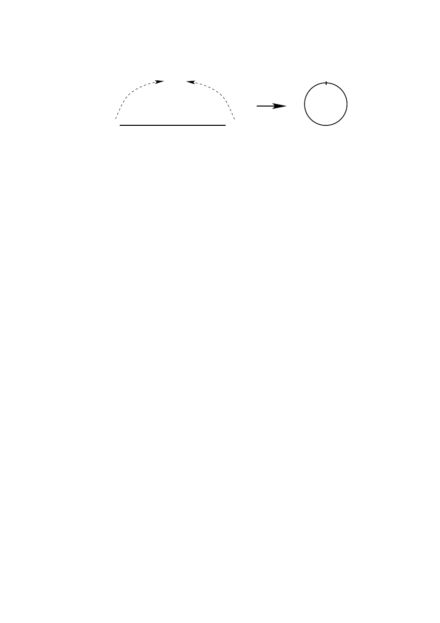
...
...
.
8
8
(a)
(b)
Fig. 9: Compactification of the real line (a) into the circumference S
1
(b) by adding the point at infinity.
single physical state
|physi. In other words, each physical state corresponds to a whole orbit of
states that are transformed among themselves by gauge transformations.
This explains the necessity of gauge fixing. In order to avoid the redundancy in the states a
further condition can be given that selects one single state on each orbit. In the case of Maxwell
electrodynamics the conditions
A
0
= 0, ~
∇ · ~
A = 0 selects a value of the gauge potential among all
possible ones giving the same value for the electric and magnetic fields.
Since states have to be identified by gauge transformations the topology of the gauge group
plays an important physical rˆole. To illustrate the point let us first deal with a toy model of a U(1)
gauge theory in 1+1 dimensions. Later we will be more general. In the Hamiltonian formalism
gauge transformations
g(~x) are functions defined on R with values on the gauge group U(1)
g : R
−→ U(1).
(4.97)
We assume that
g(x) is regular at infinity. In this case we can add to the real line R the point at
infinity to compactify it into the circumference
S
1
(see Fig. 9). Once this is done
g(x) are functions
defined on
S
1
with values on
U(1) = S
1
that can be parametrized as
g : S
1
−→ U(1),
g(x) = e
iα
(x)
,
(4.98)
with
x
∈ [0, 2π].
Because
S
1
does have a nontrivial topology,
g(x) can be divided into topological sectors.
These sectors are labelled by an integer number
n
∈ Z and are defined by
α(2π) = α(0) + 2π n .
(4.99)
Geometrically
n gives the number of times that the spatial S
1
winds around the
S
1
defining the
gauge group U(1). This winding number can be written in a more sophisticated way as
I
S
1
g(x)
−1
dg(x) = 2πn ,
(4.100)
where the integral is along the spatial
S
1
.
39

In R
3
a similar situation happens with the gauge group
8
SU(2). If we demand
g(~x)
∈ SU(2)
to be regular at infinity
|~x| → ∞ we can compactify R
3
into a three-dimensional sphere
S
3
, exactly
as we did in 1+1 dimensions. On the other hand, the function
g(~x) can be written as
g(~x) = a
0
(x)1 + ~a(x)
· ~σ
(4.101)
and the conditions
g(x)
†
g(x) = 1, det g = 1 implies that (a
0
)
2
+ ~a
2
= 1. Therefore SU(2) is a
three-dimensional sphere and
g(x) defines a function
g : S
3
−→ S
3
.
(4.102)
As it was the case in 1+1 dimensions here the gauge transformations
g(x) are also divided into
topological sectors labelled this time by the winding number
n =
1
24π
2
Z
S
3
d
3
x ǫ
ijk
Tr
g
−1
∂
i
g
g
−1
∂
i
g
g
−1
∂
i
g
∈ Z.
(4.103)
In the two cases analyzed we find that due to the nontrivial topology of the gauge group
manifold the gauge transformations are divided into different sectors labelled by an integer
n. Gauge
transformations with different values of
n cannot be smoothly deformed into each other. The sector
with
n = 0 corresponds to those gauge transformations that can be connected with the identity.
Now we can be a bit more formal. Let us consider a gauge theory in 3+1 dimensions with
gauge group
G and let us denote by
G the set of all gauge transformations G = {g : S
3
→ G}. At
the same time we define
G
0
as the set of transformations in
G that can be smoothly deformed into
the identity. Our theory will have topological sectors if
G/G
0
6= 1.
(4.104)
In the case of the electromagnetism we have seen that Gauss’ law annihilates physical states. For a
nonabelian theory the analysis is similar and leads to the condition
U(g
0
)
|physi ≡ exp
i
Z
d
3
x χ
a
(~x)~
∇ · ~
E
a
|physi = |physi,
(4.105)
where
g
0
(~x) = e
iχ
a
(~
x
)T
a
is in the connected component of the identity
G
0
. The important point
to realize here is that only the elements of
G
0
can be written as exponentials of the infinitesimal
generators. Since this generators annihilate the physical states this implies that
U(g
0
)
|physi =
|physi only when g
0
∈ G
0
.
What happens then with the other topological sectors? If
g
∈ G/G
0
there is still a unitary
operator
U(g) that realizes gauge transformations on the Hilbert space of the theory. However since
g is not in the connected component of the identity, it cannot be written as the exponential of Gauss’
law. Still gauge invariance is preserved if
U(g) only changes the overall global phase of the physical
states. For example, if
g
1
is a gauge transformation with winding number
n = 1
U(g
1
)
|physi = e
iθ
|physi.
(4.106)
8
Although we present for simplicity only the case of SU(2), similar arguments apply to any simple group.
40

It is easy to convince oneself that all transformations with winding number
n = 1 have the same
value of
θ modulo 2π. This can be shown by noticing that if g(~x) has winding number n = 1 then
g(~x)
−1
has opposite winding number
n =
−1. Since the winding number is additive, given two
transformations
g
1
,
g
2
with winding number 1,
g
−1
1
g
2
has winding number
n = 0. This implies that
|physi = U(g
−1
1
g
2
)
|physi = U(g
1
)
†
U(g
2
)
|physi = e
i
(θ
2
−θ
1
)
|physi
(4.107)
and we conclude that
θ
1
= θ
2
mod
2π. Once we know this it is straightforward to conclude that a
gauge transformation
g
n
(~x) with winding number n has the following action on physical states
U(g
n
)
|physi = e
inθ
|physi,
n
∈ Z.
(4.108)
To find a physical interpretation of this result we are going to look for similar things in other
physical situations. One of then is borrowed from condensed matter physics and refers to the quan-
tum states of electrons in the periodic potential produced by the ion lattice in a solid. For simplicity
we discuss the one-dimensional case where the minima of the potential are separated by a distance
a. When the barrier between consecutive degenerate vacua is high enough we can neglect tunnel-
ing between different vacua and consider the ground state
|nai of the potential near the minimum
located at
x = na (n
∈ Z) as possible vacua of the theory. This vacuum state is, however, not
invariant under lattice translations
e
ia b
P
|nai = |(n + 1)ai.
(4.109)
However, it is possible to define a new vacuum state
|ki =
X
n
∈Z
e
−ikna
|nai,
(4.110)
which under
e
ia b
P
transforms by a global phase
e
ia b
P
|ki =
X
n
∈Z
e
−ikna
|(n + 1)ai = e
ika
|ki.
(4.111)
This ground state is labelled by the momentum
k and corresponds to the Bloch wave function.
This looks very much the same as what we found for nonabelian gauge theories. The vacuum
state labelled by
θ plays a rˆole similar to the Bloch wave function for the periodic potential with
the identification of
θ with the momentum k. To make this analogy more precise let us write the
Hamiltonian for nonabelian gauge theories
H =
1
2
Z
d
3
x
~π
a
· ~π
a
+ ~
B
a
· ~
B
a
=
1
2
Z
d
3
x
~
E
a
· ~
E
a
+ ~
B
a
· ~
B
a
,
(4.112)
where we have used the expression of the canonical momenta
π
i
a
and we assume that the Gauss’ law
constraint is satisfied. Looking at this Hamiltonian we can interpret the first term within the brackets
as the kinetic energy
T =
1
2
~π
a
· ~π
a
and the second term as the potential energy
V =
1
2
~
B
a
· ~
B
a
.
Since
V
≥ 0 we can identify the vacua of the theory as those ~
A for which V = 0, modulo gauge
41

transformations. This happens wherever ~
A is a pure gauge. However, since we know that the gauge
transformations are labelled by the winding number we can have an infinite number of vacua which
cannot be continuously connected with one another using trivial gauge transformations. Taking a
representative gauge transformation
g
n
(~x) in the sector with winding number n, these vacua will be
associated with the gauge potentials
~
A =
1
ig
g
n
(~x)
−1
~
∇g
n
(~x),
(4.113)
modulo topologically trivial gauge transformations. Therefore the theory is characterized by an
infinite number of vacua
|ni labelled by the winding number. These vacua are not gauge invariant.
Indeed, a gauge transformation with
n = 1 will change the winding number of the vacua in one unit
U(g
1
)
|ni = |n + 1i.
(4.114)
Nevertheless a gauge invariant vacuum can be defined as
|θi =
X
n
∈Z
e
−inθ
|ni,
with
θ
∈ R
(4.115)
satisfying
U(g
1
)
|θi = e
iθ
|θi.
(4.116)
We have concluded that the nontrivial topology of the gauge group have very important phys-
ical consequences for the quantum theory. In particular it implies an ambiguity in the definition of
the vacuum. Actually, this can also be seen in a Lagrangian analysis. In constructing the Lagrangian
for the nonabelian version of Maxwell theory we only consider the term
F
a
µν
F
µν a
. However this is
not the only Lorentz and gauge invariant term that contains just two derivatives. We can write the
more general Lagrangian
L = −
1
4
F
a
µν
F
µν a
+
θ
32π
2
F
a
µν
e
F
µν a
,
(4.117)
where e
F
a
µν
is the dual of the field strength defined by
e
F
a
µν
=
1
2
ǫ
µνσλ
F
σλ
.
(4.118)
The extra term in (4.117), proportional to ~
E
a
· ~
B
a
, is actually a total derivative and does not change
the equations of motion or the quantum perturbation theory. Nevertheless it has several important
physical consequences. One of them is that it violates both parity
P and the combination of charge
conjugation and parity
CP . This means that since strong interactions are described by a nonabelian
gauge theory with group SU(3) there is an extra source of
CP violation which puts a strong bound
on the value of
θ. One of the consequences of a term like (4.117) in the QCD Lagrangian is a
42

nonvanishing electric dipole moment for the neutron [25]. The fact that this is not observed impose
a very strong bound on the value of the
θ-parameter
|θ| < 10
−9
(4.119)
From a theoretical point of view it is still to be fully understood why
θ either vanishes or has a very
small value.
Finally, the
θ-vacuum structure of gauge theories that we found in the Hamiltonian formalism
can be also obtained using path integral techniques form the Lagrangian (4.117). The second term
in Eq. (4.117) gives then a contribution that depends on the winding number of the corresponding
gauge configuration.
5
Towards computational rules: Feynman diagrams
As the basic tool to describe the physics of elementary particles, the final aim of Quantum Field
Theory is the calculation of observables. Most of the information we have about the physics of
subatomic particles comes from scattering experiments. Typically, these experiments consist of
arranging two or more particles to collide with a certain energy and to setup an array of detectors,
sufficiently far away from the region where the collision takes place, that register the outgoing
products of the collision and their momenta (together with other relevant quantum numbers).
Next we discuss how these cross sections can be computed from quantum mechanical ampli-
tudes and how these amplitudes themselves can be evaluated in perturbative Quantum Field Theory.
We keep our discussion rather heuristic and avoid technical details that can be found in standard
texts [1–10]. The techniques described will be illustrated with the calculation of the cross section
for Compton scattering at low energies.
5.1
Cross sections and S-matrix amplitudes
In order to fix ideas let us consider the simplest case of a collision experiment where two particles
collide to produce again two particles in the final state. The aim of such an experiments is a direct
measurement of the number of particles per unit time
dN
dt
(θ, ϕ) registered by the detector flying
within a solid angle
dΩ in the direction specified by the polar angles θ, ϕ (see Fig. 10). On general
grounds we know that this quantity has to be proportional to the flux of incoming particles
9
,
f
in
.
The proportionality constant defines the differential cross section
dN
dt
(θ, ϕ) = f
in
dσ
dΩ
(θ, ϕ).
(5.1)
In natural units
f
in
has dimensions of (length)
−3
, and then the differential cross section has dimen-
sions of (length)
2
. It depends, apart from the direction
(θ, ϕ), on the parameters of the collision
(energy, impact parameter, etc.) as well as on the masses and spins of the incoming particles.
Differential cross sections measure the angular distribution of the products of the collision.
It is also physically interesting to quantify how effective the interaction between the particles is to
9
This is defined as the number of particles that enter the interaction region per unit time and per unit area perpen-
dicular to the direction of the beam.
43
detector
00000000
00000000
00000000
00000000
00000000
00000000
00000000
00000000
00000000
00000000
00000000
00000000
00000000
00000000
00000000
00000000
00000000
00000000
00000000
00000000
00000000
00000000
00000000
11111111
11111111
11111111
11111111
11111111
11111111
11111111
11111111
11111111
11111111
11111111
11111111
11111111
11111111
11111111
11111111
11111111
11111111
11111111
11111111
11111111
11111111
11111111
00000000
00000000
00000000
00000000
00000000
00000000
00000000
00000000
00000000
00000000
00000000
00000000
00000000
00000000
00000000
00000000
00000000
00000000
00000000
00000000
00000000
00000000
00000000
11111111
11111111
11111111
11111111
11111111
11111111
11111111
11111111
11111111
11111111
11111111
11111111
11111111
11111111
11111111
11111111
11111111
11111111
11111111
11111111
11111111
11111111
11111111
0000000
0000000
0000000
0000000
0000000
0000000
0000000
0000000
0000000
0000000
0000000
0000000
0000000
0000000
1111111
1111111
1111111
1111111
1111111
1111111
1111111
1111111
1111111
1111111
1111111
1111111
1111111
1111111
Ω(θ,ϕ)
d
Interaction
region
detector
Fig. 10: Schematic setup of a two-to-two-particles single scattering event in the center of mass reference
frame.
produce a nontrivial dispersion. This is measured by the total cross section, which is obtained by
integrating the differential cross section over all directions
σ =
Z
1
−1
d(cos θ)
Z
2π
0
dϕ
dσ
dΩ
(θ, ϕ).
(5.2)
To get some physical intuition of the meaning of the total cross section we can think of the classical
scattering of a point particle off a sphere of radius
R. The particle undergoes a collision only when
the impact parameter is smaller than the radius of the sphere and a calculation of the total cross
section yields
σ = πR
2
. This is precisely the cross area that the sphere presents to incoming
particles.
In Quantum Mechanics in general and in Quantum Field Theory in particular the starting point
for the calculation of cross sections is the probability amplitude for the corresponding process. In a
scattering experiment one prepares a system with a given number of particles with definite momenta
~p
1
, . . . , ~p
n
. In the Heisenberg picture this is described by a time independent state labelled by the
incoming momenta of the particles (to keep things simple we consider spinless particles) that we
denote by
|~p
1
, . . . , ~p
n
; in
i.
(5.3)
On the other hand, as a result of the scattering experiment a number
k of particles with momenta
~p
1
′
, . . . , ~p
k
′
are detected. Thus, the system is now in the “out” Heisenberg picture state
|~p
1
′
, . . . , ~p
k
′
; out
i
(5.4)
44

labelled by the momenta of the particles detected at late times. The probability amplitude of detect-
ing
k particles in the final state with momenta ~p
1
′
, . . . , ~p
k
′
in the collision of
n particles with initial
momenta
~p
1
, . . . , ~p
n
defines the
S-matrix amplitude
S(in
→ out) = h~p
1
′
, . . . , ~p
k
′
; out
|~p
1
, . . . , ~p
n
; in
i.
(5.5)
It is very important to keep in mind that both the (5.3) and (5.4) are time-independent states
in the Hilbert space of a very complicated interacting theory. However, since both at early and late
times the incoming and outgoing particles are well apart from each other, the “in” and “out” states
can be thought as two states
|~p
1
, . . . , ~p
n
i and |~p
1
′
, . . . , ~p
k
′
i of the Fock space of the corresponding
free theory in which the coupling constants are zero. Then, the overlaps (5.5) can be written in terms
of the matrix elements of an
S-matrix operator b
S acting on the free Fock space
h~p
1
′
, . . . , ~p
k
′
; out
|~p
1
, . . . , ~p
n
; in
i = h~p
1
′
, . . . , ~p
k
′
| b
S
|~p
1
, . . . , ~p
n
i.
(5.6)
The operator b
S is unitary, b
S
†
= b
S
−1
, and its matrix elements are analytic in the external momenta.
In any scattering experiment there is the possibility that the particles do not interact at all and
the system is left in the same initial state. Then it is useful to write the
S-matrix operator as
b
S = 1 + i b
T ,
(5.7)
where 1 represents the identity operator. In this way, all nontrivial interactions are encoded in the
matrix elements of the
T -operator
h~p
1
′
, . . . , ~p
k
′
|i b
T
|~p
1
, . . . , ~p
n
i. Since momentum has to be con-
served, a global delta function can be factored out from these matrix elements to define the invariant
scattering amplitude
i
M
h~p
1
′
, . . . , ~p
k
′
|i b
T
|~p
1
, . . . , ~p
n
i = (2π)
4
δ
(4)
X
initial
p
i
−
X
final
p
′
f
!
i
M(~p
1
, . . . , ~p
n
; ~p
1
′
, . . . , ~p
k
′
)
(5.8)
Total and differential cross sections can be now computed from the invariant amplitudes. Here
we consider the most common situation in which two particles with momenta
~p
1
and
~p
2
collide to
produce a number of particles in the final state with momenta
~p
i
′
. In this case the total cross section
is given by
σ =
1
(2ω
p
1
)(2ω
p
2
)
|~v
12
|
Z " Y
final
states
d
3
p
′
i
(2π)
3
1
2ω
p
′
i
#
M
i
→f
2
(2π)
4
δ
(4)
p
1
+ p
2
−
X
final
states
p
′
i
!
,
(5.9)
where
~v
12
is the relative velocity of the two scattering particles. The corresponding differential cross
section can be computed by dropping the integration over the directions of the final momenta. We
will use this expression later in Section 5.3 to evaluate the cross section of Compton scattering.
We seen how particle cross sections are determined by the invariant amplitude for the corre-
sponding proccess, i.e.
S-matrix amplitudes. In general, in Quantum Field Theory it is not possible
to compute exactly these amplitudes. However, in many physical situations it can be argued that in-
teractions are weak enough to allow for a perturbative evaluation. In what follows we will describe
how
S-matrix elements can be computed in perturbation theory using Feynman diagrams and rules.
These are very convenient bookkeeping techniques allowing both to keep track of all contributions
to a process at a given order in perturbation theory, and computing the different contributions.
45
5.2
Feynman rules
The basic quantities to be computed in Quantum Field Theory are vacuum expectation values of
products of the operators of the theory. Particularly useful are time-ordered Green functions,
hΩ|T
h
O
1
(x
1
) . . .
O
n
(x
n
)
i
|Ωi,
(5.10)
where
|Ωi is the the ground state of the theory and the time ordered product is defined
T
h
O
i
(x)
O
j
(y)
i
= θ(x
0
− y
0
)
O
i
(x)
O
j
(y) + θ(y
0
− x
0
)
O
j
(y)
O
i
(x).
(5.11)
The generalization to products with more than two operators is straightforward: operators are always
multiplied in time order, those evaluated at earlier times always to the right. The interest of these
kind of correlation functions lies in the fact that they can be related to
S-matrix amplitudes through
the so-called reduction formula. To keep our discussion as simple as possible we will not derived
it or even write it down in full detail. Its form for different theories can be found in any textbook.
Here it suffices to say that the reduction formula simply states that any
S-matrix amplitude can be
written in terms of the Fourier transform of a time-ordered correlation function. Morally speaking
h~p
1
′
, . . . , ~p
m
′
; out
|~p
1
, . . . , ~p
n
; in
i
⇓
(5.12)
Z
d
4
x
1
. . .
Z
d
4
y
n
hΩ|T
h
φ(x
1
)
†
. . . φ(x
m
)
†
φ(y
1
) . . . φ(y
n
)
i
|Ωi e
ip
1′
·x
1
. . . e
−ip
n
·y
n
,
where
φ(x) is the field whose elementary excitations are the particles involved in the scattering.
The reduction formula reduces the problem of computing
S-matrix amplitudes to that of eval-
uating time-ordered correlation functions of field operators. These quantities are easy to compute
exactly in the free theory. For an interacting theory the situation is more complicated, however.
Using path integrals, the vacuum expectation value of the time-ordered product of a number of
operators can be expressed as
hΩ|T
h
O
1
(x
1
) . . .
O
n
(x
n
)
i
|Ωi =
Z
D
φDφ
†
O
1
(x
1
) . . .
O
n
(x
n
) e
iS
[φ,φ
†
]
Z
D
φDφ
†
e
iS
[φ,φ
†
]
.
(5.13)
For an theory with interactions, neither the path integral in the numerator or in the denominator is
Gaussian and they cannot be calculated exactly. However, Eq. (5.13) is still very useful. The action
S[φ, φ
†
] can be split into the free (quadratic) piece and the interaction part
S[φ, φ
†
] = S
0
[φ, φ
†
] + S
int
[φ, φ
†
].
(5.14)
All dependence in the coupling constants of the theory comes from the second piece. Expanding
now
exp[iS
int
] in power series of the coupling constant we find that each term in the series expansion
of both the numerator and the denominator has the structure
Z
D
φDφ
†
h
. . .
i
e
iS
0
[φ,φ
†
]
,
(5.15)
46
where “
. . .” denotes certain monomial of fields. The important point is that now the integration
measure only involves the free action, and the path integral in (5.15) is Gaussian and therefore can
be computed exactly. The same conclusion can be reached using the operator formalism. In this case
the correlation function (5.10) can be expressed in terms of correlation functions of operators in the
interaction picture. The advantage of using this picture is that the fields satisfy the free equations of
motion and therefore can be expanded in creation-annihilation operators. The correlations functions
are then easily computed using Wick’s theorem.
Putting together all the previous ingredients we can calculate
S-matrix amplitudes in a per-
turbative series in the coupling constants of the field theory. This can be done using Feynman
diagrams and rules, a very economical way to compute each term in the perturbative expansion of
the
S-matrix amplitude for a given process. We will not detail the the construction of Feynman rules
but just present them heuristically.
For the sake of concreteness we focus on the case of QED first. Going back to Eq. (4.70) we
expand the covariant derivative to write the action
S
QED
=
Z
d
4
x
−
1
4
F
µν
F
µν
+ ψ(i/∂
− m)ψ + eψγ
µ
ψA
µ
.
(5.16)
The action contains two types of particles, photons and fermions, that we represent by straight and
wavy lines respectively
The arrow in the fermion line does not represent the direction of the momentum but the flux of
(negative) charge. This distinguishes particles form antiparticles: if the fermion propagates from
left to right (i.e. in the direction of the charge flux) it represents a particle, whereas when it does
from right to left it corresponds to an antiparticle. Photons are not charged and therefore wavy lines
do not have orientation.
Next we turn to the interaction part of the action containing a photon field, a spinor and its
conjugate. In a Feynman diagram this corresponds to the vertex
Now, in order to compute an
S-matrix amplitude to a given order in the coupling constant e for a
process with certain number of incoming and outgoing asymptotic states one only has to draw all
possible diagrams with as many vertices as the order in perturbation theory, and the corresponding
number and type of external legs. It is very important to keep in mind that in joining the fermion
lines among the different building blocks of the diagram one has to respect their orientation. This
47

reflects the conservation of the electric charge. In addition one should only consider diagrams
that are topologically non-equivalent, i.e. that they cannot be smoothly deformed into one another
keeping the external legs fixed
10
.
To show in a practical way how Feynman diagrams are drawn, we consider Bhabha scattering,
i.e. the elastic dispersion of an electron and a positron:
e
+
+ e
−
−→ e
+
+ e
−
.
Our problem is to compute the
S-matrix amplitude to the leading order in the electric charge. Be-
cause the QED vertex contains a photon line and our process does not have photons either in the
initial or the final states we find that drawing a Feynman diagram requires at least two vertices.
In fact, the leading contribution is of order
e
2
and comes from the following two diagrams, each
containing two vertices:
e
−
e
+
e
−
e
+
+ (
−1) ×
e
−
e
+
e
−
e
+
Incoming and outgoing particles appear respectively on the left and the right of this diagram. Notice
how the identification of electrons and positrons is done comparing the direction of the charge
flux with the direction of propagation. For electrons the flux of charges goes in the direction of
propagation, whereas for positrons the two directions are opposite. These are the only two diagrams
that can be drawn at this order in perturbation theory. It is important to include a relative minus sign
between the two contributions. To understand the origin of this sign we have to remember that in
the operator formalism Feynman diagrams are just a way to encode a particular Wick contraction
of field operators in the interaction picture. The factor of
−1 reflects the relative sign in Wick
contractions represented by the two diagrams, due to the fermionic character of the Dirac field.
We have learned how to draw Feynman diagrams in QED. Now one needs to compute the
contribution of each one to the corresponding amplitude using the so-called Feynman rules. The
idea is simple: given a diagram, each of its building blocks (vertices as well as external and internal
lines) has an associated contribution that allows the calculation of the corresponding diagram. In the
case of QED in the Feynman gauge, we have the following correspondence for vertices and internal
propagators:
10
From the point of view of the operator formalism, the requirement of considering only diagrams that are topo-
logically nonequivalent comes from the fact that each diagram represents a certain Wick contraction in the correlation
function of interaction-picture operators.
48
α
β
=
⇒
i
/p
− m + iε
βα
µ
ν
=
⇒
−iη
µν
p
2
+ iε
α
β
µ
=
⇒
−ieγ
µ
βα
(2π)
4
δ
(4)
(p
1
+ p
2
+ p
3
).
A change in the gauge would reflect in an extra piece in the photon propagator. The delta function
implementing conservation of momenta is written using the convention that all momenta are enter-
ing the vertex. In addition, one has to perform an integration over all momenta running in internal
lines with the measure
Z
d
d
p
(2π)
4
,
(5.17)
and introduce a factor of
−1 for each fermion loop in the diagram
11
.
In fact, some of the integrations over internal momenta can actually be done using the delta
function at the vertices, leaving just a global delta function implementing the total momentum con-
servation in the diagram [cf. Eq. (5.8)]. It is even possible that all integrations can be eliminated
in this way. This is the case when we have tree level diagrams, i.e. those without closed loops.
In the case of diagrams with loops there will be as many remaining integrations as the number of
independent loops in the diagram.
The need to perform integrations over internal momenta in loop diagrams has important con-
sequences in Quantum Field Theory. The reason is that in many cases the resulting integrals are
ill-defined, i.e. are divergent either at small or large values of the loop momenta. In the first case
one speaks of infrared divergences and usually they cancel once all contributions to a given pro-
cess are added together. More profound, however, are the divergences appearing at large internal
momenta. These ultraviolet divergences cannot be cancelled and have to be dealt through the renor-
malization procedure. We will discuss this problem in some detail in Section 8.
Were we computing time-ordered (amputated) correlation function of operators, this would
be all. However, in the case of
S-matrix amplitudes this is not the whole story. In addition to the
11
The contribution of each diagram comes also multiplied by a degeneracy factor that takes into account in how many
ways a given Wick contraction can be done. In QED, however, these factors are equal to 1 for many diagrams.
49
previous rules here one needs to attach contributions also to the external legs in the diagram. These
are the wave functions of the corresponding asymptotic states containing information about the spin
and momenta of the incoming and outgoing particles. In the case of QED these contributions are:
Incoming fermion:
α
=
⇒
u
α
(~p, s)
Incoming antifermion:
α
=
⇒
v
α
(~p, s)
Outgoing fermion:
α
=
⇒
u
α
(~p, s)
Outgoing antifermion:
α
=
⇒
v
α
(p, s)
Incoming photon:
µ
=
⇒
ǫ
µ
(~k, λ)
Outgoing photon:
Æ
µ
=
⇒
ǫ
µ
(~k, λ)
∗
Here we have assumed that the momenta for incoming (resp. outgoing) particles are entering (resp.
leaving) the diagram. It is important also to keep in mind that in the computation of
S-matrix
amplitudes all external states are on-shell. In Section 5.3 we illustrate the use of the Feynman rules
for QED with the case of the Compton scattering.
The application of Feynman diagrams to carry out computations in perturbation theory is ex-
tremely convenient. It provides a very useful bookkeeping technique to account for all contributions
to a process at a given order in the coupling constant. This does not mean that the calculation of
Feynman diagrams is an easy task. The number of diagrams contributing to the process grows very
fast with the order in perturbation theory and the integrals that appear in calculating loop diagrams
also get very complicated. This means that, generically, the calculation of Feynman diagrams be-
yond the first few orders very often requires the use of computers.
50

Above we have illustrated the Feynman rules with the case of QED. Similar rules can be
computed for other interacting quantum field theories with scalar, vector or spinor fields. In the
case of the nonabelian gauge theories introduced in Section 4.3 we have:
α, i
β, j
=
⇒
i
/p
− m + iε
βα
δ
ij
µ, a
ν, b
=
⇒
−iη
µν
p
2
+ iε
δ
ab
α, i
β, j
µ, a
=
⇒
−igγ
µ
βα
t
a
ij
ν, b
σ, c
µ, a
=
⇒
g f
abc
h
η
µν
(p
σ
1
− p
σ
2
) + permutations
i
µ, a
σ, c
ν, b
λ, d
=
⇒
−ig
2
h
f
abe
f
cde
η
µσ
η
νλ
− η
µλ
η
νσ
+ permutations
i
It is not our aim here to give a full and detailed description of the Feynman rules for nonabelian
gauge theories. It suffices to point out that, unlike the case of QED, here the gauge fields can interact
among themselves. Indeed, the three and four gauge field vertices are a consequence of the cubic
and quartic terms in the action
S =
−
1
4
Z
d
4
x F
a
µν
F
µν a
,
(5.18)
where the nonabelian gauge field strength
F
a
µν
is given in Eq. (4.75). The self-interaction of the
51

nonabelian gauge fields has crucial dynamical consequences and its at the very heart of its success
in describing the physics of elementary particles.
5.3
An example: Compton scattering
To illustrate the use of Feynman diagrams and Feynman rules we compute the cross section for the
dispersion of photons by free electrons, the so-called Compton scattering:
γ(k, λ) + e
−
(p, s)
−→ γ(k
′
, λ
′
) + e
−
(p
′
, s
′
).
In brackets we have indicated the momenta for the different particles, as well as the polarizations and
spins of the incoming and outgoing photon and electrons respectively. The first step is to identify
all the diagrams contributing to the process at leading order. Taking into account that the vertex
of QED contains two fermion and one photon leg, it is straightforward to realize that any diagram
contributing to the process at hand must contain at least two vertices. Hence the leading contribution
is of order
e
2
. A first diagram we can draw is:
k, λ
p, s
k
′
, λ
′
p
′
, s
′
This is, however, not the only possibility. Indeed, there is a second possible diagram:
k, λ
p, s
p
′
, s
′
k
′
, λ
′
It is important to stress that these two diagrams are topologically nonequivalent, since deforming
one into the other would require changing the label of the external legs. Therefore the leading
O(e
2
)
amplitude has to be computed adding the contributions from both of them.
Using the Feynman rules of QED we find
+
= (ie)
2
u(~p
′
, s
′
)/ǫ
′
(~k
′
, λ
′
)
∗
/p + /k + m
e
(p + k)
2
− m
2
e
/ǫ(~k, λ)u(~p, s)
+ (ie)
2
u(~p
′
, s
′
)/ǫ(~k, λ)
/p
− /k
′
+ m
e
(p
− k
′
)
2
− m
2
e
/ǫ
′
(~k
′
, λ
′
)
∗
u(~p, s).
(5.19)
Because the leading order contributions only involve tree-level diagrams, there is no integration over
internal momenta and therefore we are left with a purely algebraic expression for the amplitude. To
52

get an explicit expression we begin by simplifying the numerators. The following simple identity
turns out to be very useful for this task
/a/b =
−/b/a + 2(a · b)1.
(5.20)
Indeed, looking at the first term in Eq. (5.19) we have
(/p + /k + m
e
)/ǫ(~k, λ)u(~p, s) =
−/ǫ(~k, λ)(/p − m
e
)u(~p, s) + /k/ǫ(~k, λ)u(~p, s)
+ 2p
· ǫ(~k, λ)u(~p, s),
(5.21)
where we have applied the identity (5.20) on the first term inside the parenthesis. The first term
on the right-hand side of this equation vanishes identically because of Eq. (4.35). The expression
can be further simplified if we restrict our attention to the Compton scattering at low energy when
electrons are nonrelativistic. This means that all spatial momenta are much smaller than the electron
mass
|~p|, |~k|, |~p
′
|, |~k
′
| ≪ m
e
.
(5.22)
In this approximation we have that
p
µ
, p
′µ
≈ (m
e
,~0) and therefore
p
· ǫ(~k, λ) = 0.
(5.23)
This follows from the absence of temporal photon polarization. Then we conclude that at low
energies
(/p + /k + m
e
)/ǫ(~k, λ)u(~p, s) = /k/ǫ(~k, λ)u(~p, s)
(5.24)
and similarly for the second term in Eq. (5.19)
(/p
− /k
′
+ m
e
)/ǫ
′
(~k
′
, λ
′
)
∗
u(~p, s) =
−/k
′
/ǫ
′
(~k
′
, λ
′
)
∗
u(~p, s).
(5.25)
Next, we turn to the denominators in Eq. (5.19). As it was explained in Section 5.2, in
computing scattering amplitudes incoming and outgoing particles should have on-shell momenta,
p
2
= m
2
e
= p
′2
and
k
2
= 0 = k
′2
.
(5.26)
Then, the two denominator in Eq. (5.19) simplify respectively to
(p + k)
2
− m
2
e
= p
2
+ k
2
+ 2p
· k − m
2
e
= 2p
· k = 2ω
p
|~k| − 2~p · ~k
(5.27)
and
(p
− k
′
)
2
− m
2
e
= p
2
+ k
′2
+ 2p
· k
′
− m
2
e
=
−2p · k
′
=
−2ω
p
|~k
′
| + 2~p · ~k
′
.
(5.28)
Working again in the low energy approximation (5.22) these two expressions simplify to
(p + k)
2
− m
2
e
≈ 2m
e
|~k|,
(p
− k
′
)
2
− m
2
e
≈ −2m
e
|~k
′
|.
(5.29)
53

Putting together all these expressions we find that at low energies
+
≈
(ie)
2
2m
e
u(~p
′
, s
′
)
"
/ǫ
′
(~k
′
λ
′
)
∗
/k
|~k|
ǫ(~k, λ) + ǫ(~k, λ)
/k
′
|~k
′
|
/ǫ
′
(~k
′
λ
′
)
∗
#
u(~p, s).
(5.30)
Using now again the identity (5.20) a number of times as well as the transversality condition of the
polarization vectors (4.66) we end up with a handier equation
+
≈
e
2
m
e
h
ǫ(~k, λ)
· ǫ
′
(~k
′
, λ
′
)
∗
i
u(~p
′
, s
′
)
/k
|~k|
u(~p, s)
+
e
2
2m
e
u(~p
′
, s
′
)/ǫ(~k, λ)/ǫ
′
(~k
′
, λ
′
)
∗
/k
|~k|
−
/k
′
|~k
′
|
!
u(~p, s).
(5.31)
With a little bit of effort we can show that the second term on the right-hand side vanishes. First
we notice that in the low energy limit
|~k| ≈ |~k
′
|. If in addition we make use the conservation of
momentum
k
− k
′
= p
′
− p and the identity (4.35)
u(~p
′
, s
′
)/ǫ(~k, λ)/ǫ
′
(~k
′
, λ
′
)
∗
/k
|~k|
−
/k
′
|~k
′
|
!
u(~p, s)
≈
1
|~k|
u(~p
′
, s
′
)/ǫ(~k, λ)/ǫ
′
(~k
′
, λ
′
)
∗
(/p
′
− m
e
)u(~p, s).
(5.32)
Next we use the identity (5.20) to take the term
(/p
′
− m
e
) to the right. Taking into account that in
the low energy limit the electron four-momenta are orthogonal to the photon polarization vectors
[see Eq. (5.23)] we conclude that
u(~p
′
, s
′
)/ǫ(~k, λ)/ǫ
′
(~k
′
, λ
′
)
∗
(/p
′
− m
e
)u(~p, s)
= u(~p
′
, s
′
)(/p
′
− m
e
)/ǫ(~k, λ)/ǫ
′
(~k
′
, λ
′
)
∗
u(~p, s) = 0
(5.33)
where the last identity follows from the equation satisfied by the conjugate positive-energy spinor,
u(~p
′
, s
′
)(/p
′
− m
e
) = 0.
After all these lengthy manipulations we have finally arrived at the expression of the invariant
amplitude for the Compton scattering at low energies
i
M =
e
2
m
e
h
ǫ(~k, λ)
· ǫ
′
(~k
′
, λ
′
)
∗
i
u(~p
′
, s
′
)
/k
|~k|
u(~p, s).
(5.34)
The calculation of the cross section involves computing the modulus squared of this quantity. For
many physical applications, however, one is interested in the dispersion of photons with a given po-
larization by electrons that are not polarized, i.e. whose spins are randomly distributed. In addition
in many situations either we are not interested, or there is no way to measure the final polarization
54
of the outgoing electron. This is for example the situation in cosmology, where we do not have
any information about the polarization of the free electrons in the primordial plasma before or after
the scattering with photons (although we have ways to measure the polarization of the scattered
photons).
To describe this physical situations we have to average over initial electron polarization (since
we do not know them) and sum over all possible final electron polarization (because our detector is
blind to this quantum number),
|iM|
2
=
1
2
e
2
m
e
|~k|
!
2
ǫ(~k, λ) · ǫ
′
(~k
′
, λ
′
)
∗
2
X
s
=±
1
2
X
s
′
=±
1
2
u(~p
′
, s
′
)/ku(~p, s)
2
.
(5.35)
The factor of
1
2
comes from averaging over the two possible polarizations of the incoming electrons.
The sums in this expression can be calculated without much difficulty. Expanding the absolute value
explicitly
X
s
=±
1
2
X
s
′
=±
1
2
u(~p
′
, s
′
)/ku(~p, s)
2
=
X
s
=±
1
2
X
s
′
=±
1
2
h
u(~p, s)
†
/k
†
u(~p
′
, s
′
)
†
ih
u(~p
′
, s
′
)/ku(~p, s)
i
,
(5.36)
using that
γ
µ
†
= γ
0
γ
µ
γ
0
and after some manipulation one finds that
X
s
=±
1
2
X
s
′
=±
1
2
u(~p
′
, s
′
)/ku(~p, s)
2
=
X
s
=±
1
2
u
α
(~p, s)u
β
(~p, s)
(/k)
βσ
X
s
′
=±
1
2
u
σ
(~p
′
, s
′
)u
ρ
(~p
′
, s
′
)
(/k)
ρα
= Tr
h
(/p + m
e
)/k(/p
′
+ m
e
)/k
i
,
(5.37)
where the final expression has been computed using the completeness relations in Eq. (4.38). The
final evaluation of the trace can be done using the standard Dirac matrices identities. Here we
compute it applying again the relation (5.20) to commute
/p
′
and
/k. Using that k
2
= 0 and that we
are working in the low energy limit we have
12
Tr
h
(/p + m
e
)/k(/p
′
+ m
e
)/k
i
= 2(p
· k)(p
′
· k)Tr 1 ≈ 8m
2
e
|~k|
2
.
(5.38)
This gives the following value for the invariant amplitude
|iM|
2
= 4e
4
ǫ(~k, λ) · ǫ
′
(~k
′
, λ
′
)
∗
2
(5.39)
Plugging
|iM|
2
into the formula for the differential cross section we get
dσ
dΩ
=
1
64π
2
m
2
e
|iM|
2
=
e
2
4πm
e
2
ǫ(~k, λ) · ǫ
′
(~k
′
, λ
′
)
∗
2
.
(5.40)
12
We use also the fact that the trace of the product of an odd number of Dirac matrices is always zero.
55
The prefactor of the last equation is precisely the square of the so-called classical electron radius
r
cl
. In fact, the previous differential cross section can be rewritten as
dσ
dΩ
=
3
8π
σ
T
ǫ(~k, λ) · ǫ
′
(~k
′
, λ
′
)
∗
2
,
(5.41)
where
σ
T
is the total Thomson cross section
σ
T
=
e
4
6πm
2
e
=
8π
3
r
2
cl
.
(5.42)
The result (5.41) is relevant in many areas of Physics, but its importance is paramount in the
study of the cosmological microwave background (CMB). Just before recombination the universe is
filled by a plasma of electrons interacting with photons via Compton scattering, with temperatures
of the order of 1 keV. Electrons are then nonrelativistic (
m
e
∼ 0.5 MeV) and the approximations
leading to Eq. (5.41) are fully valid. Because we do not know the polarization state of the photons
before being scattered by electrons we have to consider the cross section averaged over incoming
photon polarizations. From Eq. (5.41) we see that this is proportional to
1
2
X
λ
=1,2
ǫ(~k, λ) · ǫ
′
(~k
′
, λ
′
)
∗
2
=
"
1
2
X
λ
=1,2
ǫ
i
(~k, λ)ǫ
j
(~k, λ)
∗
#
ǫ
j
(~k
′
, λ
′
)ǫ
i
(~k
′
, λ
′
)
∗
.
(5.43)
The sum inside the brackets can be computed using the normalization of the polarization vectors,
|~ǫ (~k, λ)|
2
= 1, and the transversality condition ~k
· ~ǫ(~k, λ) = 0
1
2
X
λ
=1,2
ǫ(~k, λ) · ǫ
′
(~k
′
, λ
′
)
∗
2
=
1
2
δ
ij
−
k
i
k
j
|~k|
2
!
ǫ
′
j
(~k
′
, λ
′
)ǫ
′
i
(~k
′
, λ
′
)
∗
=
1
2
h
1
− |~ℓ · ~ǫ
′
(~k
′
, λ
′
)
|
2
i
,
(5.44)
where ~
ℓ =
~
k
|~k|
is the unit vector in the direction of the incoming photon.
From the last equation we conclude that Thomson scattering suppresses all polarizations par-
allel to the direction of the incoming photon ~
ℓ, whereas the differential cross section reaches the
maximum in the plane normal to ~
ℓ. If photons would collide with the electrons in the plasma with
the same intensity from all directions, the result would be an unpolarized CMB radiation. The
fact that polarization is actually measured in the CMB carries crucial information about the physics
of the plasma before recombination and, as a consequence, about the very early universe (see for
example [21] for a throughout discussion).
6
Symmetries
6.1
Noether’s theorem
In Classical Mechanics and Classical Field Theory there is a basic result that relates symmetries and
conserved charges. This is called Noether’s theorem and states that for each continuous symmetry
56
of the system there is conserved current. In its simplest version in Classical Mechanics it can be
easily proved. Let us consider a Lagrangian
L(q
i
, ˙q
i
) which is invariant under a transformation
q
i
(t)
→ q
′
i
(t, ǫ) labelled by a parameter ǫ. This means that L(q
′
, ˙q
′
) = L(q, ˙q) without using the
equations of motion
13
. If
ǫ
≪ 1 we can consider an infinitesimal variation of the coordinates δ
ǫ
q
i
(t)
and the invariance of the Lagrangian implies
0 = δ
ǫ
L(q
i
, ˙q
i
) =
∂L
∂q
i
δ
ǫ
q
i
+
∂L
∂ ˙q
i
δ
ǫ
˙q
i
=
∂L
∂q
i
−
d
dt
∂L
∂ ˙q
i
δ
ǫ
q
i
+
d
dt
∂L
∂ ˙q
i
δ
ǫ
q
i
.
(6.1)
When
δ
ǫ
q
i
is applied on a solution to the equations of motion the term inside the square brackets
vanishes and we conclude that there is a conserved quantity
˙
Q = 0
with
Q
≡
∂L
∂ ˙q
i
δ
ǫ
q
i
.
(6.2)
Notice that in this derivation it is crucial that the symmetry depends on a continuous parameter since
otherwise the infinitesimal variation of the Lagrangian in Eq. (6.1) does not make sense.
In Classical Field Theory a similar result holds. Let us consider for simplicity a theory of
a single field
φ(x). We say that the variations δ
ǫ
φ depending on a continuous parameter ǫ are a
symmetry of the theory if, without using the equations of motion, the Lagrangian density changes
by
δ
ǫ
L = ∂
µ
K
µ
.
(6.3)
If this happens then the action remains invariant and so do the equations of motion. Working out
now the variation of
L under δ
ǫ
φ we find
∂
µ
K
µ
=
∂
L
∂(∂
µ
φ)
∂
µ
δ
ǫ
φ +
∂
L
∂φ
δ
ǫ
φ = ∂
µ
∂
L
∂(∂
µ
φ)
δ
ǫ
φ
+
∂
L
∂φ
− ∂
µ
∂
L
∂(∂
µ
φ)
δ
ǫ
φ.
(6.4)
If
φ(x) is a solution to the equations of motion the last terms disappears, and we find that there is a
conserved current
∂
µ
J
µ
= 0
with
J
µ
=
∂
L
∂(∂
µ
φ)
δ
ǫ
φ
− K
µ
.
(6.5)
Actually a conserved current implies the existence of a charge
Q
≡
Z
d
3
x J
0
(t, ~x)
(6.6)
which is conserved
dQ
dt
=
Z
d
3
x ∂
0
J
0
(t, ~x) =
−
Z
d
3
x ∂
i
J
i
(t, ~x) = 0,
(6.7)
13
The following result can be also derived a more general situations where the Lagrangian changes by a total time
derivative.
57
provided the fields vanish at infinity fast enough. Moreover, the conserved charge
Q is a Lorentz
scalar. After canonical quantization the charge
Q defined by Eq. (6.6) is promoted to an operator
that generates the symmetry on the fields
δφ = i[φ, Q].
(6.8)
As an example we can consider a scalar field
φ(x) which under a coordinate transformation
x
→ x
′
changes as
φ
′
(x
′
) = φ(x). In particular performing a space-time translation x
µ
′
= x
µ
+ a
µ
we have
φ
′
(x)
− φ(x) = −a
µ
∂
µ
φ +
O(a
2
)
=
⇒
δφ =
−a
µ
∂
µ
φ.
(6.9)
Since the Lagrangian density is also a scalar quantity, it transforms under translations as
δ
L = −a
µ
∂
µ
L.
(6.10)
Therefore the corresponding conserved charge is
J
µ
=
−
∂
L
∂(∂
µ
φ)
a
ν
∂
ν
φ + a
µ
L ≡ −a
ν
T
µν
,
(6.11)
where we introduced the energy-momentum tensor
T
µν
=
∂
L
∂(∂
µ
φ)
∂
ν
φ
− η
µν
L.
(6.12)
We find that associated with the invariance of the theory with respect to space-time translations
there are four conserved currents defined by
T
µν
with
ν = 0, . . . , 3, each one associated with the
translation along a space-time direction. These four currents form a rank-two tensor under Lorentz
transformations satisfying
∂
µ
T
µν
= 0.
(6.13)
The associated conserved charges are given by
P
ν
=
Z
d
3
x T
0ν
(6.14)
and correspond to the total energy-momentum content of the field configuration. Therefore the
energy density of the field is given by
T
00
while
T
0i
is the momentum density. In the quantum
theory the
P
µ
are the generators of space-time translations.
Another example of a symmetry related with a physically relevant conserved charge is the
global phase invariance of the Dirac Lagrangian (4.27),
ψ
→ e
iθ
ψ. For small θ this corresponds to
variations
δ
θ
ψ = iθψ, δ
θ
ψ =
−iθψ which by Noether’s theorem result in the conserved charge
j
µ
= ψγ
µ
ψ,
∂
µ
j
µ
= 0.
(6.15)
58
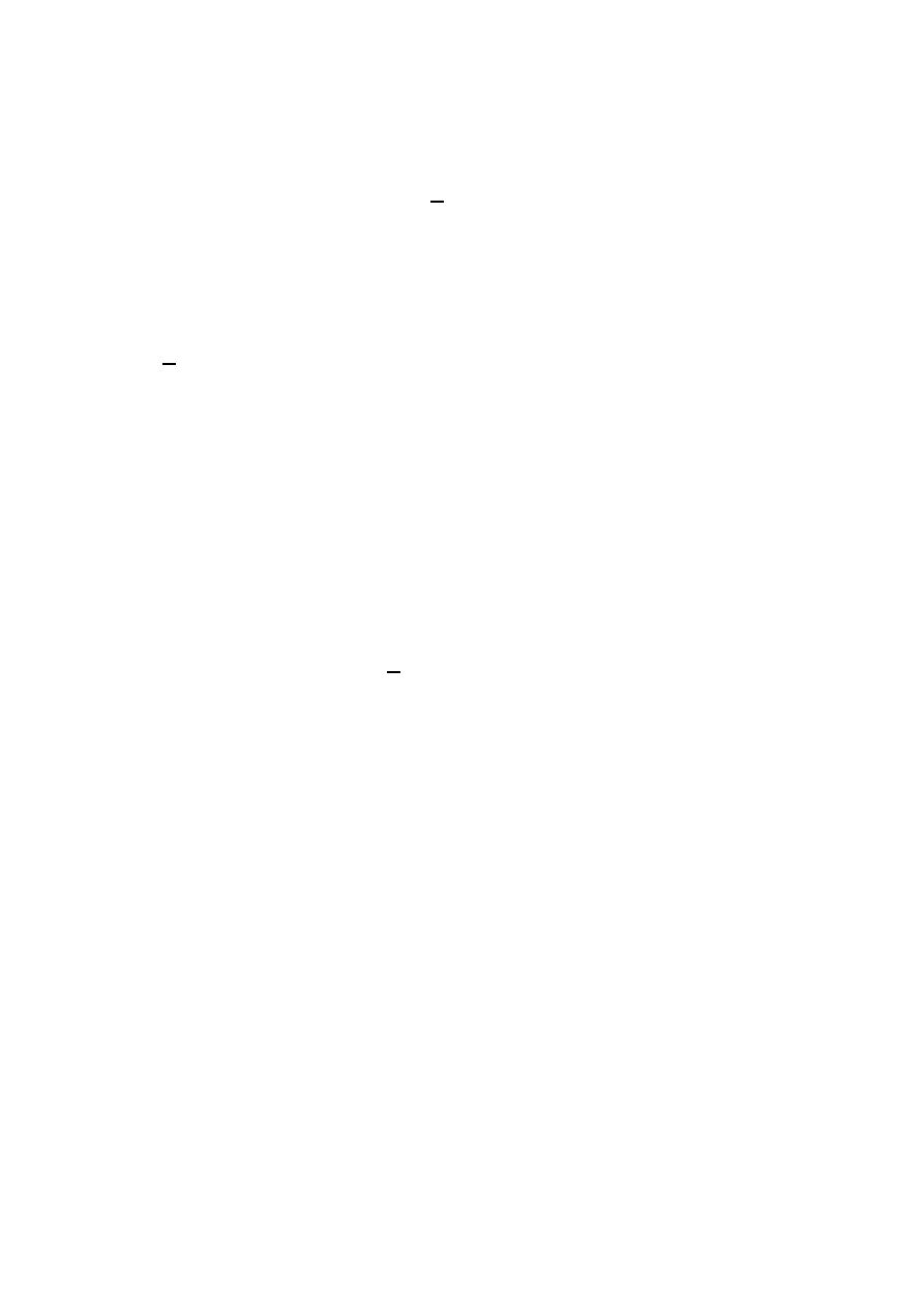
Thus implying the existence of a conserved charge
Q =
Z
d
3
xψγ
0
ψ =
Z
d
3
xψ
†
ψ.
(6.16)
In physics there are several instances of global U(1) symmetries that act as phase shifts on spinors.
This is the case, for example, of the baryon and lepton number conservation in the Standard Model.
A more familiar case is the U(1) local symmetry associated with electromagnetism. Notice that
although in this case we are dealing with a local symmetry,
θ
→ eα(x), the invariance of the
Lagrangian holds in particular for global transformations and therefore there is a conserved current
j
µ
= eψγ
µ
ψ. In Eq. (4.72) we saw that the spinor is coupled to the photon field precisely through
this current. Its time component is the electric charge density
ρ, while the spatial components are
the current density vector
~.
This analysis can be carried over also to nonabelian unitary global symmetries acting as
ψ
i
−→ U
ij
ψ
j
,
U
†
U = 1
(6.17)
and leaving invariant the Dirac Lagrangian when we have several fermions. If we write the matrix
U in terms of the hermitian group generators T
a
as
U = exp (iα
a
T
a
) ,
(T
a
)
†
= T
a
,
(6.18)
we find the conserved current
j
µ a
= ψ
i
T
a
ij
γ
µ
ψ
j
,
∂
µ
j
µ
= 0.
(6.19)
This is the case, for example of the approximate flavor symmetries in hadron physics. The simplest
example is the isospin symmetry that mixes the quarks
u and d
u
d
−→ M
u
d
,
M
∈ SU(2).
(6.20)
Since the proton is a bound state of two quarks
u and one quark d while the neutron is made out
of one quark
u and two quarks d, this isospin symmetry reduces at low energies to the well known
isospin transformations of nuclear physics that mixes protons and neutrons.
6.2
Symmetries in the quantum theory
We have seen that in canonical quantization the conserved charges
Q
a
associated to symmetries
by Noether’s theorem are operators implementing the symmetry at the quantum level. Since the
charges are conserved they must commute with the Hamiltonian
[Q
a
, H] = 0.
(6.21)
There are several possibilities in the quantum mechanical realization of a symmetry:
59
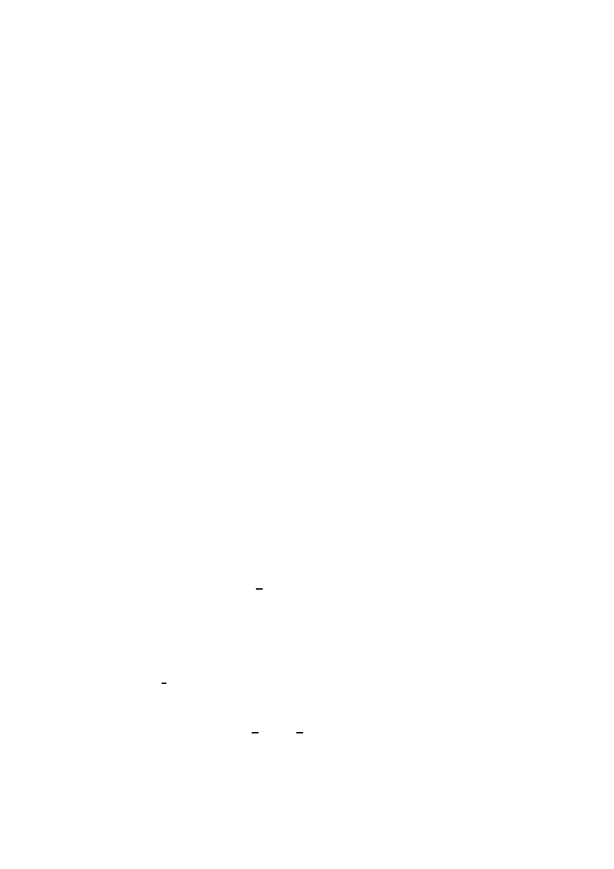
Wigner-Weyl realization. In this case the ground state of the theory
|0i is invariant under the
symmetry. Since the symmetry is generated by
Q
a
this means that
U(α)|0i ≡ e
iα
a
Q
a
|0i = |0i
=
⇒
Q
a
|0i = 0.
(6.22)
At the same time the fields of the theory have to transform according to some irreducible represen-
tation of the group generated by the
Q
a
. From Eq. (6.8) it is easy to prove that
U(α)φ
i
U(α)
−1
= U
ij
(α)φ
j
,
(6.23)
where
U
ij
(α) is an element of the representation in which the field φ
i
transforms. If we consider
now the quantum state associated with the operator
φ
i
|ii = φ
i
|0i
(6.24)
we find that because of the invariance of the vacuum (6.22) the states
|ii transform in the same
representation as
φ
i
U(α)|ii = U(α)φ
i
U(α)
−1
U(α)|0i = U
ij
(α)φ
j
|0i = U
ij
(α)
|ji.
(6.25)
Therefore the spectrum of the theory is classified in multiplets of the symmetry group. In addition,
since
[H,
U(α)] = 0 all states in the same multiplet have the same energy. If we consider one-
particle states, then going to the rest frame we conclude that all states in the same multiplet have
exactly the same mass.
Nambu-Goldstone realization. In our previous discussion the result that the spectrum of
the theory is classified according to multiplets of the symmetry group depended crucially on the
invariance of the ground state. However this condition is not mandatory and one can relax it to
consider theories where the vacuum state is not left invariant by the symmetry
e
iα
a
Q
a
|0i 6= |0i
=
⇒
Q
a
|0i 6= 0.
(6.26)
In this case it is also said that the symmetry is spontaneously broken by the vacuum.
To illustrate the consequences of (6.26) we consider the example of a number scalar fields
ϕ
i
(
i = 1, . . . , N) whose dynamics is governed by the Lagrangian
L =
1
2
∂
µ
ϕ
i
∂
µ
ϕ
i
− V (ϕ),
(6.27)
where we assume that
V (φ) is bounded from below. This theory is globally invariant under the
transformations
δϕ
i
= ǫ
a
(T
a
)
i
j
ϕ
j
,
(6.28)
with
T
a
,
a = 1, . . . ,
1
2
N(N
− 1) the generators of the group SO(N).
To analyze the structure of vacua of the theory we construct the Hamiltonian
H =
Z
d
3
x
1
2
π
i
π
i
+
1
2
~
∇ϕ
i
· ~∇ϕ
i
+ V (ϕ)
(6.29)
60
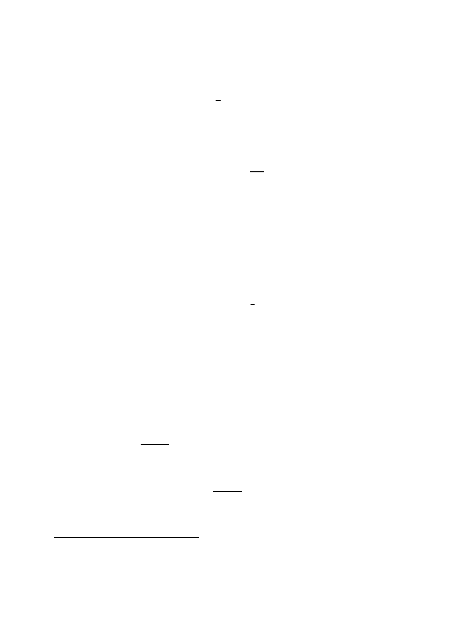
and look for the minimum of
V(ϕ) =
Z
d
3
x
1
2
~
∇ϕ
i
· ~∇ϕ
i
+ V (ϕ)
.
(6.30)
Since we are interested in finding constant field configurations, ~
∇ϕ = ~0 to preserve translational
invariance, the vacua of the potential
V(ϕ) coincides with the vacua of V (ϕ). Therefore the minima
of the potential correspond to the vacuum expectation values
14
hϕ
i
i :
V (
hϕ
i
i) = 0,
∂V
∂ϕ
i
ϕ
i
=hϕ
i
i
= 0.
(6.31)
We divide the generators
T
a
of SO(
N) into two groups: Those denoted by H
α
(
α = 1, . . . , h)
that satisfy
(H
α
)
i
j
hϕ
j
i = 0.
(6.32)
This means that the vacuum configuration
hϕ
i
i is left invariant by the transformation generated
by
H
α
. For this reason we call them unbroken generators. Notice that the commutator of two
unbroken generators also annihilates the vacuum expectation value,
[H
α
, H
β
]
ij
hϕ
j
i = 0. Therefore
the generators
{H
α
} form a subalgebra of the algebra of the generators of SO(N). The subgroup of
the symmetry group generated by them is realized `a la Wigner-Weyl.
The remaining generators
K
A
, with
A = 1, . . . ,
1
2
N(N
− 1) − h, by definition do not preserve
the vacuum expectation value of the field
(K
A
)
i
j
hϕ
j
i 6= 0.
(6.33)
These will be called the broken generators. Next we prove a very important result concerning
the broken generators known as the Goldstone theorem: for each generator broken by the vacuum
expectation value there is a massless excitation.
The mass matrix of the excitations around the vacuum
hϕ
i
i is determined by the quadratic
part of the potential. Since we assumed that
V (
hϕi) = 0 and we are expanding around a minimum,
the first term in the expansion of the potential
V (ϕ) around the vacuum expectation values is given
by
V (ϕ) =
∂
2
V
∂ϕ
i
∂ϕ
j
ϕ
=hϕi
(ϕ
i
− hϕ
i
i)(ϕ
j
− hϕ
j
i) + O
(ϕ
− hϕi)
3
(6.34)
and the mass matrix is:
M
2
ij
≡
∂
2
V
∂ϕ
i
∂ϕ
j
ϕ
=hϕi
.
(6.35)
In order to avoid a cumbersome notation we do not show explicitly the dependence of the mass
matrix on the vacuum expectation values
hϕ
i
i.
14
For simplicity we consider that the minima of V
(φ) occur at zero potential.
61
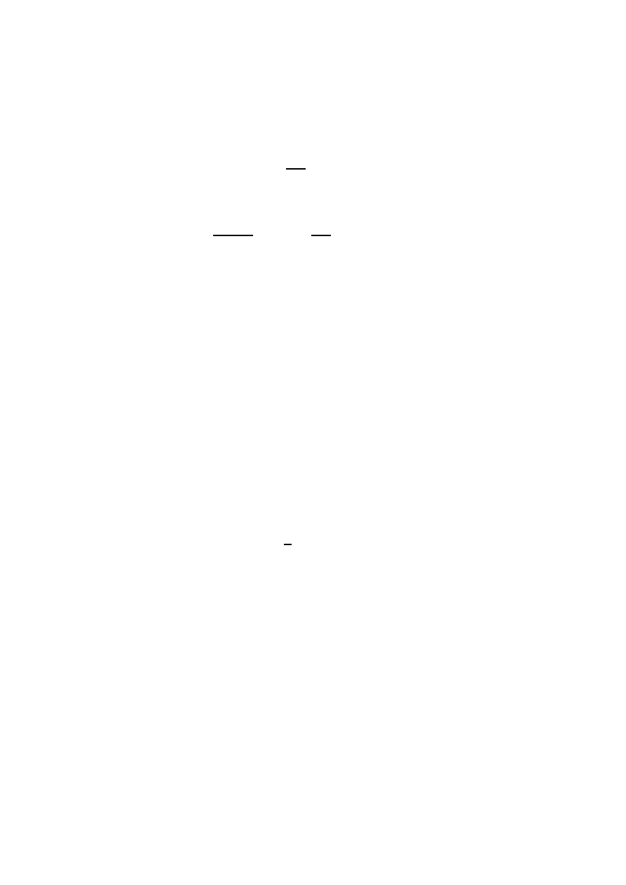
To extract some information about the possible zero modes of the mass matrix, we write down
the conditions that follow from the invariance of the potential under
δϕ
i
= ǫ
a
(T
a
)
i
j
ϕ
j
. At first order
in
ǫ
a
δV (ϕ) = ǫ
a
∂V
∂ϕ
i
(T
a
)
i
j
ϕ
j
= 0.
(6.36)
Differentiating this expression with respect to
ϕ
k
we arrive at
∂
2
V
∂ϕ
i
∂ϕ
k
(T
a
)
i
j
ϕ
j
+
∂V
∂ϕ
i
(T
a
)
i
k
= 0.
(6.37)
Now we evaluate this expression in the vacuum
ϕ
i
=
hϕ
i
i. Then the derivative in the second term
cancels while the second derivative in the first one gives the mass matrix. Hence we find
M
2
ik
(T
a
)
i
j
hϕ
j
i = 0.
(6.38)
Now we can write this expression for both broken and unbroken generators. For the unbroken ones,
since
(H
α
)
i
j
hϕ
j
i = 0, we find a trivial identity 0 = 0. On the other hand for the broken generators
we have
M
2
ik
(K
A
)
i
j
hϕ
j
i = 0.
(6.39)
Since
(K
A
)
i
j
hϕ
j
i 6= 0 this equation implies that the mass matrix has as many zero modes as broken
generators. Therefore we have proven Goldstone’s theorem: associated with each broken symmetry
there is a massless mode in the theory. Here we have presented a classical proof of the theorem. In
the quantum theory the proof follows the same lines as the one presented here but one has to consider
the effective action containing the effects of the quantum corrections to the classical Lagrangian.
As an example to illustrate this theorem, we consider a SO(3) invariant scalar field theory with
a “mexican hat” potential
V (~
ϕ) =
λ
4
~
ϕ
2
− a
2
2
.
(6.40)
The vacua of the theory correspond to the configurations satisfying
h~ϕi
2
= a
2
. In field space
this equation describes a two-dimensional sphere and each solution is just a point in that sphere.
Geometrically it is easy to visualize that a given vacuum field configuration, i.e. a point in the
sphere, is preserved by SO(2) rotations around the axis of the sphere that passes through that point.
Hence the vacuum expectation value of the scalar field breaks the symmetry according to
h~ϕi :
SO(3)
−→ SO(2).
(6.41)
Since SO(3) has three generators and SO(2) only one we see that two generators are broken and
therefore there are two massless Goldstone bosons. Physically this massless modes can be thought
of as corresponding to excitations along the surface of the sphere
h~ϕi
2
= a
2
.
Once a minimum of the potential has been chosen we can proceed to quantize the excitations
around it. Since the vacuum only leaves invariant a SO(2) subgroup of the original SO(3) symmetry
62

group it seems that the fact that we are expanding around a particular vacuum expectation value of
the scalar field has resulted in a lost of symmetry. This is however not the case. The full quantum
theory is symmetric under the whole symmetry group SO(3). This is reflected in the fact that the
physical properties of the theory do not depend on the particular point of the sphere
h~ϕi
2
= a
2
that
we have chosen. Different vacua are related by the full SO(3) symmetry and therefore should give
the same physics.
It is very important to realize that given a theory with a vacuum determined by
h~ϕi all other
possible vacua of the theory are unaccessible in the infinite volume limit. This means that two
vacuum states
|0
1
i, |0
2
i corresponding to different vacuum expectation values of the scalar field are
orthogonal
h0
1
|0
2
i = 0 and cannot be connected by any local observable Φ(x), h0
1
|Φ(x)|0
2
i = 0.
Heuristically this can be understood by noticing that in the infinite volume limit switching from one
vacuum into another one requires changing the vacuum expectation value of the field everywhere
in space at the same time, something that cannot be done by any local operator. Notice that this is
radically different to our expectations based on the Quantum Mechanics of a system with a finite
number of degrees of freedom.
In High Energy Physics the typical example of a Goldstone boson is the pion, associated with
the spontaneous breaking of the global chiral isospin
SU(2)
L
× SU(2)
R
symmetry. This symmetry
acts independently in the left- and right-handed spinors as
u
L,R
d
L,R
−→ M
L,R
u
L,R
d
L,R
,
M
L,R
∈ SU(2)
L,R
(6.42)
Presumably since the quarks are confined at low energies this symmetry is spontaneously broken
down to the diagonal SU(2) acting in the same way on the left- and right-handed components of
the spinors. Associated with this symmetry breaking there is a Goldstone mode which is identified
as the pion. Notice, nevertheless, that the SU(2)
L
×SU(2)
R
would be an exact global symmetry of
the QCD Lagrangian only in the limit when the masses of the quarks are zero
m
u
, m
d
→ 0. Since
these quarks have nonzero masses the chiral symmetry is only approximate and as a consequence
the corresponding Goldstone boson is not massless. That is why pions have masses, although they
are the lightest particle among the hadrons.
Symmetry breaking appears also in many places in condensed matter. For example, when a
solid crystallizes from a liquid the translational invariance that is present in the liquid phase is broken
to a discrete group of translations that represent the crystal lattice. This symmetry breaking has
Goldstone bosons associated which are identified with phonons which are the quantum excitation
modes of the vibrational degrees of freedom of the lattice.
The Higgs mechanism. Gauge symmetry seems to prevent a vector field from having a mass.
This is obvious once we realize that a term in the Lagrangian like
m
2
A
µ
A
µ
is incompatible with
gauge invariance.
However certain physical situations seem to require massive vector fields. This happened for
example during the 1960s in the study of weak interactions. The Glashow model gave a common
description of both electromagnetic and weak interactions based on a gauge theory with group
SU(2)
×U(1) but, in order to reproduce Fermi’s four-fermion theory of the β-decay it was necessary
that two of the vector fields involved would be massive. Also in condensed matter physics massive
63
vector fields are required to describe certain systems, most notably in superconductivity.
The way out to this situation is found in the concept of spontaneous symmetry breaking dis-
cussed previously. The consistency of the quantum theory requires gauge invariance, but this in-
variance can be realized `a la Nambu-Goldstone. When this is the case the full gauge symmetry is
not explicitly present in the effective action constructed around the particular vacuum chosen by the
theory. This makes possible the existence of mass terms for gauge fields without jeopardizing the
consistency of the full theory, which is still invariant under the whole gauge group.
To illustrate the Higgs mechanism we study the simplest example, the Abelian Higgs model:
a U(1) gauge field coupled to a self-interacting charged complex scalar field
Φ with Lagrangian
L = −
1
4
F
µν
F
µν
+ D
µ
ΦD
µ
Φ
−
λ
4
ΦΦ
− µ
2
2
,
(6.43)
where the covariant derivative is given by Eq. (4.69). This theory is invariant under the gauge
transformations
Φ
→ e
iα
(x)
Φ,
A
µ
→ A
µ
+ ∂
µ
α(x).
(6.44)
The minimum of the potential is defined by the equation
|Φ| = µ. We have a continuum of different
vacua labelled by the phase of the scalar field. None of these vacua, however, is invariant under the
gauge symmetry
hΦi = µe
iϑ
0
→ µe
iϑ
0
+iα(x)
(6.45)
and therefore the symmetry is spontaneously broken Let us study now the theory around one of
these vacua, for example
hΦi = µ, by writing the field Φ in terms of the excitations around this
particular vacuum
Φ(x) =
µ +
1
√
2
σ(x)
e
iϑ
(x)
.
(6.46)
Independently of whether we are expanding around a particular vacuum for the scalar field we
should keep in mind that the whole Lagrangian is still gauge invariant under (6.44). This means that
performing a gauge transformation with parameter
α(x) =
−ϑ(x) we can get rid of the phase in
Eq. (6.46). Substituting then
Φ(x) = µ +
1
√
2
σ(x) in the Lagrangian we find
L = −
1
4
F
µν
F
µν
+ e
2
µ
2
A
µ
A
µ
+
1
2
∂
µ
σ∂
µ
σ
−
1
2
λµ
2
σ
2
− λµσ
3
−
λ
4
σ
4
+ e
2
µA
µ
A
µ
σ + e
2
A
µ
A
µ
σ
2
.
(6.47)
What are the excitation of the theory around the vacuum
hΦi = µ? First we find a massive real
scalar field
σ(x). The important point however is that the vector field A
µ
now has a mass given by
m
2
γ
= 2e
2
µ
2
.
(6.48)
64

The remarkable thing about this way of giving a mass to the photon is that at no point we have given
up gauge invariance. The symmetry is only hidden. Therefore in quantizing the theory we can still
enjoy all the advantages of having a gauge theory but at the same time we have managed to generate
a mass for the gauge field.
It is surprising, however, that in the Lagrangian (6.47) we did not found any massless mode.
Since the vacuum chosen by the scalar field breaks the
U(1) generator of U(1) we would have
expected one masless particle from Goldstone’s theorem. To understand the fate of the missing
Goldstone boson we have to revisit the calculation leading to Eq. (6.47). Were we dealing with a
global U(1) theory, the Goldstone boson would correspond to excitation of the scalar field along the
valley of the potential and the phase
ϑ(x) would be the massless Goldstone boson. However we have
to keep in mind that in computing the Lagrangian we managed to get rid of
ϑ(x) by shifting it into
A
µ
using a gauge transformation. Actually by identifying the gauge parameter with the Goldstone
excitation we have completely fixed the gauge and the Lagrangian (6.47) does not have any gauge
symmetry left.
A massive vector field has three polarizations: two transverse ones ~
k
· ~ǫ (~k, ±1) = 0 plus a
longitudinal one
~ǫ
L
(~k)
∼ ~k. In gauging away the massless Goldstone boson ϑ(x) we have trans-
formed it into the longitudinal polarization of the massive vector field. In the literature this is usually
expressed saying that the Goldstone mode is “eaten up” by the longitudinal component of the gauge
field. It is important to realize that in spite of the fact that the Lagrangian (6.47) looks pretty dif-
ferent from the one we started with we have not lost any degrees of freedom. We started with the
two polarizations of the photon plus the two degrees of freedom associated with the real and imag-
inary components of the complex scalar field. After symmetry breaking we end up with the three
polarizations of the massive vector field and the degree of freedom of the real scalar field
σ(x).
We can also understand the Higgs mechanism in the light of our discussion of gauge symme-
try in section 4.4. In the Higgs mechanism the invariance of the theory under infinitesimal gauge
transformations is not explicitly broken, and this implies that Gauss’ law is satisfied quantum me-
chanically, ~
∇ · ~
E
a
|physi = 0. The theory remains invariant under gauge transformations in the
connected component of the identity
G
0
, the ones generated by Gauss’ law. This does not pose any
restriction on the possible breaking of the invariance of the theory with respect to transformations
that cannot be continuously deformed to the identity. Hence in the Higgs mechanism the invariance
under gauge transformation that are not in the connected component of the identity,
G/G
0
, can be
broken. Let us try to put it in more precise terms. As we learned in section 4.4, in the Hamiltonian
formulation of the theory finite energy gauge field configurations tend to a pure gauge at spatial
infinity
~
A
µ
(~x)
−→
1
ig
g(~x)
−1
~
∇g(~x),
|~x| → ∞
(6.49)
The set transformations
g
0
(~x)
∈ G
0
that tend to the identity at infinity are the ones generated by
Gauss’ law. However, one can also consider in general gauge transformations
g(~x) which, as
|~x| →
∞, approach any other element g ∈ G. The quotient G
∞
≡ G/G
0
gives a copy of the gauge group
at infinity. There is no reason, however, why this group should not be broken, and in general it is if
the gauge symmetry is spontaneously broken. Notice that this is not a threat to the consistency of
65
the theory. Properties like the decoupling of unphysical states are guaranteed by the fact that Gauss’
law is satisfied quantum mechanically and are not affected by the breaking of
G
∞
.
The Abelian Higgs model discussed here can be regarded as a toy model of the Higgs mech-
anism responsible for giving mass to the
W
±
and
Z
0
gauge bosons in the Standard Model. In
condensed matter physics the symmetry breaking described by the nonrelativistic version of the
Abelian Higgs model can be used to characterize the onset of a superconducting phase in the BCS
theory, where the complex scalar field
Φ is associated with the Cooper pairs. In this case the param-
eter
µ
2
depends on the temperature. Above the critical temperature
T
c
,
µ
2
(T ) > 0 and there is only
a symmetric vacuum
hΦi = 0. When, on the other hand, T < T
c
then
µ
2
(T ) < 0 and symmetry
breaking takes place. The onset of a nonzero mass of the photon (6.48) below the critical tem-
perature explains the Meissner effect: the magnetic fields cannot penetrate inside superconductors
beyond a distance of the order
1
m
γ
.
7
Anomalies
So far we did not worry too much about how classical symmetries of a theory are carried over to the
quantum theory. We have implicitly assumed that classical symmetries are preserved in the process
of quantization, so they are also realized in the quantum theory.
This, however, does not have to be necessarily the case. Quantizing an interacting field theory
is a very involved process that requires regularization and renormalization and sometimes, it does
not matter how hard we try, there is no way for a classical symmetry to survive quantization. When
this happens one says that the theory has an anomaly (for a review see [27]). It is important to avoid
here the misconception that anomalies appear due to a bad choice of the way a theory is regularized
in the process of quantization. When we talk about anomalies we mean a classical symmetry that
cannot be realized in the quantum theory, no matter how smart we are in choosing the regularization
procedure.
In the following we analyze some examples of anomalies associated with global and local
symmetries of the classical theory. In Section 8 we will encounter yet another example of an
anomaly, this time associated with the breaking of classical scale invariance in the quantum the-
ory.
7.1
Axial anomaly
Probably the best known examples of anomalies appear when we consider axial symmetries. If we
consider a theory of two Weyl spinors
u
±
L = iψ∂/ψ = iu
†
+
σ
µ
+
∂
µ
u
+
+ iu
†
−
σ
µ
−
∂
µ
u
−
with
ψ =
u
+
u
−
(7.1)
the Lagrangian is invariant under two types of global U(1) transformations. In the first one both
helicities transform with the same phase, this is a vector transformation:
U(1)
V
: u
±
−→ e
iα
u
±
,
(7.2)
66

whereas in the second one, the axial
U(1), the signs of the phases are different for the two chiralities
U(1)
A
: u
±
−→ e
±iα
u
±
.
(7.3)
Using Noether’s theorem, there are two conserved currents, a vector current
J
µ
V
= ψγ
µ
ψ = u
†
+
σ
µ
+
u
+
+ u
†
−
σ
µ
−
u
−
=
⇒
∂
µ
J
µ
V
= 0
(7.4)
and an axial vector current
J
µ
A
= ψγ
µ
γ
5
ψ = u
†
+
σ
µ
+
u
+
− u
†
−
σ
µ
−
u
−
=
⇒
∂
µ
J
µ
A
= 0.
(7.5)
The theory described by the Lagrangian (7.1) can be coupled to the electromagnetic field.
The resulting classical theory is still invariant under the vector and axial U(1) symmetries (7.2) and
(7.3). Surprisingly, upon quantization it turns out that the conservation of the axial current (7.5) is
spoiled by quantum effects
∂
µ
J
µ
A
∼ ~ ~
E
· ~
B.
(7.6)
To understand more clearly how this result comes about we study first a simple model in
two dimensions that captures the relevant physics involved in the four-dimensional case [28]. We
work in Minkowski space in two dimensions with coordinates
(x
0
, x
1
)
≡ (t, x) and where the
spatial direction is compactified to a circle
S
1
. In this setup we consider a fermion coupled to the
electromagnetic field. Notice that since we are living in two dimensions the field strength
F
µν
only
has one independent component that corresponds to the electric field along the spatial direction,
F
01
≡ E (in two dimensions there are no magnetic fields!).
To write the Lagrangian for the spinor field we need to find a representation of the algebra of
γ-matrices
{γ
µ
, γ
ν
} = 2η
µν
with
η =
1
0
0
−1
.
(7.7)
In two dimensions the dimension of the representation of the
γ-matrices is 2
[
2
2
]
= 2. Here take
γ
0
≡ σ
1
=
0 1
1 0
,
γ
1
≡ iσ
2
=
0 1
−1 0
.
(7.8)
This is a chiral representation since the matrix
γ
5
is diagonal
15
γ
5
≡ −γ
0
γ
1
=
1
0
0
−1
(7.9)
Writing the two-component spinor
ψ as
ψ =
u
+
u
−
(7.10)
15
In any even number of dimensions γ
5
is defined to satisfy the conditions γ
2
5
= 1 and
{γ
5
, γ
µ
} = 0.
67
+
−
p
p
E
E
v
v
Fig. 11: Spectrum of the massless two-dimensional Dirac field.
and defining as usual the projectors
P
±
=
1
2
(1
± γ
5
) we find that the components u
±
of
ψ are
respectively a right- and left-handed Weyl spinor in two dimensions.
Once we have a representation of the
γ-matrices we can write the Dirac equation. Expressing
it in terms of the components
u
±
of the Dirac spinor we find
(∂
0
− ∂
1
)u
+
= 0,
(∂
0
+ ∂
1
)u
−
= 0.
(7.11)
The general solution to these equations can be immediately written as
u
+
= u
+
(x
0
+ x
1
),
u
−
= u
−
(x
0
− x
1
).
(7.12)
Hence
u
±
are two wave packets moving along the spatial dimension respectively to the left
(u
+
)
and to the right
(u
−
). Notice that according to our convention the left-moving u
+
is a right-handed
spinor (positive helicity) whereas the right-moving
u
−
is a left-handed spinor (negative helicity).
If we want to interpret (7.11) as the wave equation for two-dimensional Weyl spinors we have
the following wave functions for free particles with well defined momentum
p
µ
= (E, p).
u
(E)
±
(x
0
± x
1
) =
1
√
L
e
−iE(x
0
±x
1
)
with
p =
∓E.
(7.13)
As it is always the case with the Dirac equation we have both positive and negative energy solutions.
For
u
+
, since
E =
−p, we see that the solutions with positive energy are those with negative
momentum
p < 0, whereas the negative energy solutions are plane waves with p > 0. For the
left-handed spinor
u
−
the situation is reversed. Besides, since the spatial direction is compact with
length
L the momentum p is quantized according to
p =
2πn
L
,
n
∈ Z.
(7.14)
68
p
E
E
p
0,+
0,−
Fig. 12: Vacuum of the theory.
The spectrum of the theory is represented in Fig. 11.
Once we have the spectrum of the theory the next step is to obtain the vacuum. As with the
Dirac equation in four dimensions we fill all the states with
E
≤ 0 (Fig. 12). Exciting of a particle
in the Dirac see produces a positive energy fermion plus a hole that is interpreted as an antiparticle.
This gives us the clue on how to quantize the theory. In the expansion of the operator
u
±
in terms of
the modes (7.13) we associate positive energy states with annihilation operators whereas the states
with negative energy are associated with creation operators for the corresponding antiparticle
u
±
(x) =
X
E>
0
h
a
±
(E)v
(E)
±
(x) + b
†
±
(E)v
(E)
±
(x)
∗
i
.
(7.15)
The operator
a
±
(E) acting on the vacuum
|0, ±i annihilates a particle with positive energy E and
momentum
∓E. In the same way b
†
±
(E) creates out of the vacuum an antiparticle with positive
energy
E and spatial momentum
∓E. In the Dirac sea picture the operator b
±
(E)
†
is originally an
annihilation operator for a state of the sea with negative energy
−E. As in the four-dimensional
case the problem of the negative energy states is solved by interpreting annihilation operators for
negative energy states as creation operators for the corresponding antiparticle with positive energy
(and vice versa). The operators appearing in the expansion of
u
±
in Eq. (7.15) satisfy the usual
algebra
{a
λ
(E), a
†
λ
′
(E
′
)
} = {b
λ
(E), b
†
λ
′
(E
′
)
} = δ
E,E
′
δ
λλ
′
,
(7.16)
where we have introduced the label
λ, λ
′
=
±. Also, a
λ
(E), a
†
λ
(E) anticommute with b
λ
′
(E
′
),
b
†
λ
′
(E
′
).
The Lagrangian of the theory
L = iu
†
+
(∂
0
+ ∂
1
)u
+
+ iu
†
−
(∂
0
− ∂
1
)u
−
(7.17)
69

is invariant under both U(1)
V
, Eq. (7.2), and U(1)
A
, Eq. (7.3). The associated Noether currents are
in this case
J
µ
V
=
u
†
+
u
+
+ u
†
−
u
−
−u
†
+
u
+
+ u
†
−
u
−
,
J
µ
A
=
u
†
+
u
+
− u
†
−
u
−
−u
†
+
u
+
− u
†
−
u
−
.
(7.18)
The associated conserved charges are given, for the vector current by
Q
V
=
Z
L
0
dx
1
u
†
+
u
+
+ u
†
−
u
−
(7.19)
and for the axial current
Q
A
=
Z
L
0
dx
1
u
†
+
u
+
− u
†
−
u
−
.
(7.20)
Using the orthonormality relations for the modes
v
(E)
±
(x)
Z
L
0
dx
1
v
(E)
±
(x) v
(E
′
)
±
(x) = δ
E,E
′
(7.21)
we find for the conserved charges:
Q
V
=
X
E>
0
h
a
†
+
(E)a
+
(E)
− b
†
+
(E)b
+
(E) + a
†
−
(E)a
−
(E)
− b
†
−
(E)b
−
(E)
i
,
Q
A
=
X
E>
0
h
a
†
+
(E)a
+
(E)
− b
†
+
(E)b
+
(E)
− a
†
−
(E)a
−
(E) + b
†
−
(E)b
−
(E)
i
.
(7.22)
We see that
Q
V
counts the net number (particles minus antiparticles) of positive helicity states plus
the net number of states with negative helicity. The axial charge, on the other hand, counts the
net number of positive helicity states minus the number of negative helicity ones. In the case of
the vector current we have subtracted a formally divergent vacuum contribution to the charge (the
“charge of the Dirac sea”).
In the free theory there is of course no problem with the conservation of either
Q
V
or
Q
A
,
since the occupation numbers do not change. What we want to study is the effect of coupling the
theory to electric field
E. We work in the gauge A
0
= 0. Instead of solving the problem exactly we
are going to simulate the electric field by adiabatically varying in a long time
τ
0
the vector potential
A
1
from zero value to
−Eτ
0
. From our discussion in section 4.3 we know that the effect of the
electromagnetic coupling in the theory is a shift in the momentum according to
p
−→ p − eA
1
,
(7.23)
where
e is the charge of the fermions. Since we assumed that the vector potential varies adiabati-
cally, we can assume it to be approximately constant at each time.
Then, we have to understand what is the effect of (7.23) on the vacuum depicted in Fig.
(12). What we find is that the two branches move as shown in Fig. (13) resulting in some of
70
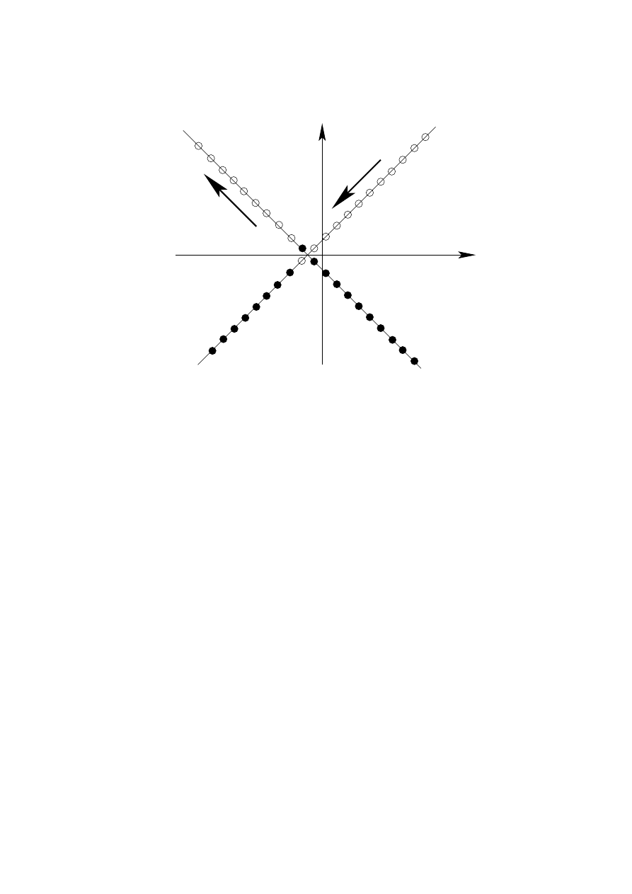
p
E
Fig. 13: Effect of the electric field.
the negative energy states of the
v
+
branch acquiring positive energy while the same number of
the empty positive energy states of the other branch
v
−
will become empty negative energy states.
Physically this means that the external electric field
E creates a number of particle-antiparticle pairs
out of the vacuum. Denoting by
N
∼ eE the number of such pairs created by the electric field per
unit time, the final values of the charges
Q
V
and
Q
A
are
Q
A
(τ
0
) = (N
− 0) + (0 − N) = 0,
Q
V
(τ
0
) = (N
− 0) − (0 − N) = 2N.
(7.24)
Therefore we conclude that the coupling to the electric field produces a violation in the conservation
of the axial charge per unit time given by
∆Q
A
∼ eE. This implies that
∂
µ
J
µ
A
∼ e~E,
(7.25)
where we have restored ~ to make clear that the violation in the conservation of the axial current is
a quantum effect. At the same time
∆Q
V
= 0 guarantees that the vector current remains conserved
also quantum mechanically,
∂
µ
J
µ
V
= 0.
We have just studied a two-dimensional example of the Adler-Bell-Jackiw axial anomaly [29].
The heuristic analysis presented here can be made more precise by computing the quantity
C
µν
=
h0|T [J
µ
A
(x)J
ν
V
(0)]
|0i =
J
µ
A
γ
(7.26)
71

The anomaly is given then by
∂
µ
C
µν
. A careful calculation yields the numerical prefactor missing
in Eq. (7.25) leading to the result
∂
µ
J
µ
A
=
e~
2π
ε
νσ
F
νσ
,
(7.27)
with
ε
01
=
−ε
10
= 1.
The existence of an anomaly in the axial symmetry that we have illustrated in two dimensions
is present in all even dimensional of space-times. In particular in four dimensions the axial anomaly
it is given by
∂
µ
J
µ
A
=
−
e
2
16π
2
ε
µνσλ
F
µν
F
σλ
.
(7.28)
This result has very important consequences in the physics of strong interactions as we will see in
what follows
7.2
Chiral symmetry in QCD
Our knowledge of the physics of strong interactions is based on the theory of Quantum Chromo-
dynamics (QCD) [31]. This is a nonabelian gauge theory with gauge group SU(
N
c
) coupled to a
number
N
f
of quarks. These are spin-
1
2
particles
Q
i f
labelled by two quantum numbers: color
i = 1, . . . , N
c
and flavor
f = 1, . . . , N
f
. The interaction between them is mediated by the
N
2
c
− 1
gauge bosons, the gluons
A
a
µ
,
a = 1, . . . , N
2
c
− 1. In the real world N
c
= 3 and the number of
flavors is six, corresponding to the number of different quarks: up (
u), down (d), charm (c), strange
(
s), top (t) and bottom (b).
For the time being we are going to study a general theory of QCD with
N
c
colors and
N
f
flavors. Also, for reasons that will be clear later we are going to work in the limit of vanishing quark
masses,
m
f
→ 0. In this cases the Lagrangian is given by
L
QCD
=
−
1
4
F
a
µν
F
a µν
+
N
f
X
f
=1
h
iQ
f
L
D
/ Q
f
L
+ iQ
f
R
D
/ Q
f
R
i
,
(7.29)
where the subscripts
L and R indicate respectively left and right-handed spinors, Q
f
L,R
≡ P
±
Q
f
,
and the field strength
F
a
µν
and the covariant derivative
D
µ
are respectively defined in Eqs. (4.75)
and (4.78). Apart from the gauge symmetry, this Lagrangian is also invariant under a global
U(
N
f
)
L
×U(N
f
)
R
acting on the flavor indices and defined by
U(
N
f
)
L
:
Q
f
L
→
P
f
′
(U
L
)
f f
′
Q
f
′
L
Q
f
R
→ Q
f
R
U(
N
f
)
R
:
Q
f
L
→ Q
f
L
Q
r
R
→
P
f
′
(U
R
)
f f
′
Q
f
′
R
(7.30)
with
U
L
, U
R
∈ U(N
f
). Actually, since U(N)=U(1)
×SU(N) this global symmetry group can be
written as SU(
N
f
)
L
× SU(N
f
)
R
× U(1)
L
× U(1)
R
. The abelian subgroup U(1)
L
× U(1)
R
can be now
72
decomposed into their vector U(1)
B
and axial U(1)
A
subgroups defined by the transformations
U(1)
B
:
Q
f
L
→ e
iα
Q
f
L
Q
f
R
→ e
iα
Q
f
R
U(1)
A
:
Q
f
L
→ e
iα
Q
f
L
Q
f
R
→ e
−iα
Q
f
R
(7.31)
According to Noether’s theorem, associated with these two abelian symmetries we have two con-
served currents:
J
µ
V
=
N
f
X
f
=1
Q
f
γ
µ
Q
f
,
J
µ
A
=
N
f
X
f
=1
Q
f
γ
µ
γ
5
Q
f
.
(7.32)
The conserved charge associated with vector charge
J
µ
V
is actually the baryon number defined as
the number of quarks minus number of antiquarks.
The nonabelian part of the global symmetry group SU(
N
f
)
L
×SU(N
f
)
R
can also be decom-
posed into its vector and axial subgroups, SU(
N
f
)
V
× SU(N
f
)
A
, defined by the following transfor-
mations of the quarks fields
SU(
N
f
)
V
:
Q
f
L
→
P
f
′
(U
L
)
f f
′
Q
f
′
L
Q
f
R
→
P
f
′
(U
L
)
f f
′
Q
f
′
R
SU(
N
f
)
A
:
Q
f
L
→
P
f
′
(U
L
)
f f
′
Q
f
′
L
Q
f
R
→
P
f
′
(U
−1
R
)
f f
′
Q
f
′
R
(7.33)
Again, the application of Noether’s theorem shows the existence of the following nonabelian con-
served charges
J
I µ
V
≡
N
f
X
f,f
′
=1
Q
f
γ
µ
(T
I
)
f f
′
Q
f
′
,
J
I µ
A
≡
N
f
X
f,f
′
=1
Q
f
γ
µ
γ
5
(T
I
)
f f
′
Q
f
′
.
(7.34)
To summarize, we have shown that the initial chiral symmetry of the QCD Lagrangian (7.29) can
be decomposed into its chiral and vector subgroups according to
U(
N
f
)
L
× U(N
f
)
R
= SU(N
f
)
V
× SU(N
f
)
A
× U(1)
B
× U(1)
A
.
(7.35)
The question to address now is which part of the classical global symmetry is preserved by the
quantum theory.
As argued in section 7.1, the conservation of the axial currents
J
µ
A
and
J
a µ
A
can in principle be
spoiled due to the presence of an anomaly. In the case of the abelian axial current
J
µ
A
the relevant
quantity is the correlation function
C
µνσ
≡ h0|T
J
µ
A
(x)j
a ν
gauge
(x
′
)j
b σ
gauge
(0)
|0i =
N
f
X
f
=1
J
µ
A
Q
f
g
Q
f
g
Q
f
symmetric
(7.36)
73

Here
j
a µ
gauge
is the nonabelian conserved current coupling to the gluon field
j
a µ
gauge
≡
N
f
X
f
=1
Q
f
γ
µ
τ
a
Q
f
,
(7.37)
where, to avoid confusion with the generators of the global symmetry we have denoted by
τ
a
the
generators of the gauge group SU(
N
c
). The anomaly can be read now from
∂
µ
C
µνσ
. If we impose
Bose symmetry with respect to the interchange of the two outgoing gluons and gauge invariance of
the whole expression,
∂
ν
C
µνσ
= 0 = ∂
σ
C
µνσ
, we find that the axial abelian global current has an
anomaly given by
16
∂
µ
J
µ
A
=
−
g
2
N
f
32π
2
ε
µνσλ
F
a
µν
F
a µν
.
(7.38)
In the case of the nonabelian axial global symmetry SU(
N
f
)
A
the calculation of the anomaly
is made as above. The result, however, is quite different since in this case we conclude that the non-
abelian axial current
J
a µ
A
is not anomalous. This can be easily seen by noticing that associated with
the axial current vertex we have a generator
T
I
of SU(
N
f
), whereas for the two gluon vertices we
have the generators
τ
a
of the gauge group SU(
N
c
). Therefore, the triangle diagram is proportional
to the group-theoretic factor
J
Iµ
A
Q
f
g
Q
f
g
Q
f
symmetric
∼ tr T
I
tr
{τ
a
, τ
b
} = 0
(7.39)
which vanishes because the generators of SU(
N
f
) are traceless.
From here we would conclude that the nonabelian axial symmetry SU(
N
f
)
A
is nonanomalous.
However this is not the whole story since quarks are charged particles that also couple to photons.
Hence there is a second potential source of an anomaly coming from the the one-loop triangle
diagram coupling
J
I µ
A
to two photons
h0|T
h
J
I µ
A
(x)j
ν
em
(x
′
)j
σ
em
(0)
i
|0i =
N
f
X
f
=1
J
Iµ
A
Q
f
γ
Q
f
γ
Q
f
symmetric
(7.40)
where
j
µ
em
is the electromagnetic current
j
µ
em
=
N
f
X
f
=1
q
f
Q
f
γ
µ
Q
f
,
(7.41)
16
The normalization of the generators T
I
of the global SU(N
f
) is given by
tr (T
I
T
J
) =
1
2
δ
IJ
.
74
with
q
f
the electric charge of the
f -th quark flavor. A calculation of the diagram in (7.40) shows the
existence of an Adler-Bell-Jackiw anomaly given by
∂
µ
J
I µ
A
=
−
N
c
16π
2
N
f
X
f
=1
(T
I
)
f f
q
2
f
ε
µνσλ
F
µν
F
σλ
,
(7.42)
where
F
µν
is the field strength of the electromagnetic field coupling to the quarks. The only chance
for the anomaly to cancel is that the factor between brackets in this equation be identically zero.
Before proceeding let us summarize the results found so far. Because of the presence of
anomalies the axial part of the global chiral symmetry, SU(
N
f
)
A
and U(1)
A
are not realized quantum
mechanically in general. We found that U(1)
A
is always affected by an anomaly. However, because
the right-hand side of the anomaly equation (7.38) is a total derivative, the anomalous character of
J
µ
A
does not explain the absence of U(1)
A
multiplets in the hadron spectrum, since a new current
can be constructed which is conserved. In addition, the nonexistence of candidates for a Goldstone
boson associated with the right quantum numbers indicates that U(1)
A
is not spontaneously broken
either, so it has be explicitly broken somehow. This is the so-called U(1)-problem which was solved
by ’t Hooft [32], who showed how the contribution of quantum transitions between vacua with
topologically nontrivial gauge field configurations (instantons) results in an explicit breaking of this
symmetry.
Due to the dynamics of the SU(
N
c
) gauge theory the axial nonabelian symmetry is sponta-
neously broken due to the presence at low energies of a vacuum expectation value for the fermion
bilinear
Q
f
Q
f
h0|Q
f
Q
f
|0i 6= 0
(No summation in
f !).
(7.43)
This nonvanishing vacuum expectation value for the quark bilinear actually breaks chiral invari-
ance spontaneously to the vector subgroup SU(
N
f
)
V
, so the only subgroup of the original global
symmetry that is realized by the full theory at low energy is
U(
N
f
)
L
× U(N
f
)
R
−→ SU(N
f
)
V
× U(1)
B
.
(7.44)
Associated with this breaking a Goldstone boson should appear with the quantum numbers of the
broken nonabelian current. For example, in the case of QCD the Goldstone bosons associated
with the spontaneously symmetry breaking induced by the vacuum expectation values
huui, hddi
and
h(ud − du)i have been identified as the pions π
0
,
π
±
. These bosons are not exactly massless
because of the nonvanishing mass of the
u and d quarks. Since the global chiral symmetry is already
slightly broken by mass terms in the Lagrangian, the associated Goldstone bosons also have masses
although they are very light compared to the masses of other hadrons.
In order to have a better physical understanding of the role of anomalies in the physics of
strong interactions we particularize now our analysis of the case of real QCD. Since the
u and d
quarks are much lighter than the other four flavors, QCD at low energies can be well described
by including only these two flavors and ignoring heavier quarks. In this approximation, from our
previous discussion we know that the low energy global symmetry of the theory is SU(2)
V
×U(1)
B
,
75
where now the vector group SU(2)
V
is the well-known isospin symmetry. The axial U(1)
A
current
is anomalous due to Eq. (7.38) with
N
f
= 2. In the case of the nonabelian axial symmetry SU(2)
A
,
taking into account that
q
u
=
2
3
e and q
d
=
−
1
3
e and that the three generators of SU(2) can be written
in terms of the Pauli matrices as
T
K
=
1
2
σ
K
we find
X
f
=u,d
(T
1
)
f f
q
2
f
=
X
f
=u,d
(T
1
)
f f
q
2
f
= 0,
X
f
=u,d
(T
3
)
f f
q
2
f
=
e
2
6
.
(7.45)
Therefore
J
3 µ
A
is anomalous.
Physically, the anomaly in the axial current
J
3 µ
A
has an important consequence. In the quark
model, the wave function of the neutral pion
π
0
is given in terms of those for the
u and d quark by
|π
0
i =
1
√
2
|¯ui|ui − | ¯
d
i|di
.
(7.46)
The isospin quantum numbers of
|π
0
i are those of the generator T
3
. Actually the analogy goes
further since
∂
µ
J
3 µ
A
is the operator creating a pion
π
0
out of the vacuum
|π
0
i ∼ ∂
µ
J
3 µ
A
|0i.
(7.47)
This leads to the physical interpretation of the triangle diagram (7.40) with
J
3 µ
A
as the one loop
contribution to the decay of a neutral pion into two photons
π
0
−→ 2γ .
(7.48)
This is an interesting piece of physics. In 1967 Sutherland and Veltman [33] presented a
calculation, using current algebra techniques, according to which the decay of the pion into two
photons should be suppressed. This however contradicted the experimental evidence that showed
the existence of such a decay. The way out to this paradox, as pointed out in [29], is the axial
anomaly. What happens is that the current algebra analysis overlooks the ambiguities associated
with the regularization of divergences in Quantum Field Theory. A QED evaluation of the triangle
diagram leads to a divergent integral that has to be regularized somehow. It is in this process that
the Adler-Bell-Jackiw axial anomaly appears resulting in a nonvanishing value for the
π
0
→ 2γ
amplitude
17
.
The existence of anomalies associated with global currents does not necessarily mean diffi-
culties for the theory. On the contrary, as we saw in the case of the axial anomaly it is its existence
what allows for a solution of the Sutherland-Veltman paradox and an explanation of the electromag-
netic decay of the pion. The situation, however, is very different if we deal with local symmetries.
A quantum mechanical violation of gauge symmetry leads to all kinds of problems, from lack of
renormalizability to nondecoupling of negative norm states. This is because the presence of an
anomaly in the theory implies that the Gauss’ law constraint ~
∇ · ~
E
a
= ρ
a
cannot be consistently
17
An early computation of the triangle diagram for the electromagnetic decay of the pion was made by Steinberger
in [30].
76
implemented in the quantum theory. As a consequence states that classically are eliminated by the
gauge symmetry become propagating fields in the quantum theory, thus spoiling the consistency of
the theory.
Anomalies in a gauge symmetry can be expected only in chiral theories where left and right-
handed fermions transform in different representations of the gauge group. Physically, the most
interesting example of such theories is the electroweak sector of the Standard Model where, for
example, left handed fermions transform as doublets under SU(2) whereas right-handed fermions
are singlets. On the other hand, QCD is free of gauge anomalies since both left- and right-handed
quarks transform in the fundamental representation of SU(3).
We consider the Lagrangian
L = −
1
4
F
a µν
F
a
µν
+ i
N
+
X
i
=1
ψ
i
+
D
/
(+)
ψ
i
+
+ i
N
−
X
j
=1
ψ
j
−
D
/
(−)
ψ
j
−
,
(7.49)
where the chiral fermions
ψ
i
±
transform according to the representations
τ
a
i,
±
of the gauge group
G
(
a = 1, . . . , dim G). The covariant derivatives D
(±)
µ
are then defined by
D
(±)
µ
ψ
i
±
= ∂
µ
ψ
i
±
+ igA
K
µ
τ
K
i,
±
ψ
i
±
.
(7.50)
As for global symmetries, anomalies in the gauge symmetry appear in the triangle diagram with one
axial and two vector gauge current vertices
h0|T
j
a µ
A
(x)j
b ν
V
(x
′
)j
c σ
V
(0)
|0i =
j
aµ
A
j
bν
V
j
cσ
V
symmetric
(7.51)
where gauge vector and axial currents
j
a µ
V
,
j
a µ
A
are given by
j
aµ
V
=
N
+
X
i
=1
ψ
i
+
τ
a
+
γ
µ
ψ
i
+
+
N
−
X
j
=1
ψ
j
−
τ
a
−
γ
µ
ψ
j
−
,
j
aµ
A
=
N
+
X
i
=1
ψ
i
+
τ
a
+
γ
µ
ψ
i
+
−
N
−
X
i
=1
ψ
j
−
τ
a
−
γ
µ
ψ
j
−
.
(7.52)
Luckily, we do not have to compute the whole diagram in order to find an anomaly cancellation
condition, it is enough if we calculate the overall group theoretical factor. In the case of the diagram
in Eq. (7.51) for every fermion species running in the loop this factor is equal to
tr
τ
a
i,
±
{τ
b
i,
±
, τ
c
i,
±
}
,
(7.53)
77
where the sign
± corresponds respectively to the generators of the representation of the gauge group
for the left and right-handed fermions. Hence the anomaly cancellation condition reads
N
+
X
i
=1
tr
τ
a
i,
+
{τ
b
i,
+
, τ
c
i,
+
}
−
N
−
X
j
=1
tr
τ
a
j,
−
{τ
b
j,
−
, τ
c
j,
−
}
= 0.
(7.54)
Knowing this we can proceed to check the anomaly cancellation in the Standard Model
SU(3)
×SU(2)×U(1). Left handed fermions (both leptons and quarks) transform as doublets with
respect to the SU(2) factor whereas the right-handed components are singlets. The charge with
respect to the U(1) part, the hypercharge
Y , is determined by the Gell-Mann-Nishijima formula
Q = T
3
+ Y,
(7.55)
where
Q is the electric charge of the corresponding particle and T
3
is the eigenvalue with respect
to the third generator of the SU(2) group in the corresponding representation:
T
3
=
1
2
σ
3
for the
doublets and
T
3
= 0 for the singlets. For the first family of quarks (u, d) and leptons (e, ν
e
) we have
the following field content
quarks:
u
α
d
α
L,
1
6
u
α
R,
2
3
d
α
R,
2
3
leptons:
ν
e
e
L,
−
1
2
e
R,
−1
(7.56)
where
α = 1, 2, 3 labels the color quantum number and the subscript indicates the value of the weak
hypercharge
Y . Denoting the representations of SU(3)
×SU(2)×U(1) by (n
c
, n
w
)
Y
, with
n
c
and
n
w
the representations of SU(3) and SU(2) respectively and
Y the hypercharge, the matter content of
the Standard Model consists of a three family replication of the representations:
left-handed fermions:
(3, 2)
L
1
6
(1, 2)
L
−
1
2
(7.57)
right-handed fermions:
(3, 1)
R
2
3
(3, 1)
R
−
1
3
(1, 1)
R
−1
.
In computing the triangle diagram we have 10 possibilities depending on which factor of the gauge
group SU(3)
×SU(2)×U(1) couples to each vertex:
SU(3)
3
SU(2)
3
U(1)
3
SU(3)
2
SU(2)
SU(2) U(1)
SU(3)
2
U(1)
SU(2) U(1)
2
SU(3) SU(2)
2
SU(3) SU(2) U(1)
SU(3) U(1)
2
78
It is easy to check that some of them do not give rise to anomalies. For example the anomaly for
the SU(3)
3
case cancels because left and right-handed quarks transform in the same representation.
In the case of SU(2)
3
the cancellation happens term by term because of the Pauli matrices identity
σ
a
σ
b
= δ
ab
+ iε
abc
σ
c
that leads to
tr
σ
a
{σ
b
, σ
c
}
= 2 (tr σ
a
) δ
bc
= 0.
(7.58)
However the hardest anomaly cancellation condition to satisfy is the one with three U(1)’s. In this
case the absence of anomalies within a single family is guaranteed by the nontrivial identity
X
left
Y
3
+
−
X
right
Y
3
−
= 3
× 2 ×
1
6
3
+ 2
×
−
1
2
3
− 3 ×
2
3
3
− 3 ×
−
1
3
3
− (−1)
3
=
−
3
4
+
3
4
= 0.
(7.59)
It is remarkable that the anomaly exactly cancels between leptons and quarks. Notice that this result
holds even if a right-handed sterile neutrino is added since such a particle is a singlet under the whole
Standard Model gauge group and therefore does not contribute to the triangle diagram. Therefore
we see how the matter content of the Standard Model conspires to yield a consistent quantum field
theory.
In all our discussion of anomalies we only considered the computation of one-loop diagrams.
It may happen that higher loop orders impose additional conditions. Fortunately this is not so: the
Adler-Bardeen theorem [34] guarantees that the axial anomaly only receives contributions from one
loop diagrams. Therefore, once anomalies are canceled (if possible) at one loop we know that there
will be no new conditions coming from higher-loop diagrams in perturbation theory.
The Adler-Bardeen theorem, however, only applies in perturbation theory. It is nonetheless
possible that nonperturbative effects can result in the quantum violation of a gauge symmetry. This
is precisely the case pointed out by Witten [35] with respect to the SU(2) gauge symmetry of the
Standard Model. In this case the problem lies in the nontrivial topology of the gauge group SU(2).
The invariance of the theory with respect to gauge transformations which are not in the connected
component of the identity makes all correlation functions equal to zero. Only when the number of
left-handed SU(2) fermion doublets is even gauge invariance allows for a nontrivial theory. It is
again remarkable that the family structure of the Standard Model makes this anomaly to cancel
3
×
u
d
L
+ 1
×
ν
e
e
L
= 4 SU(2)-doublets,
(7.60)
where the factor of 3 comes from the number of colors.
8
Renormalization
8.1
Removing infinities
From its very early stages, Quantum Field Theory was faced with infinities. They emerged in the
calculation of most physical quantities, such as the correction to the charge of the electron due to
79

the interactions with the radiation field. The way these divergences where handled in the 1940s,
starting with Kramers, was physically very much in the spirit of the Quantum Theory emphasis in
observable quantities: since the observed magnitude of physical quantities (such as the charge of the
electron) is finite, this number should arise from the addition of a “bare” (unobservable) value and
the quantum corrections. The fact that both of these quantities were divergent was not a problem
physically, since only its finite sum was an observable quantity. To make thing mathematically
sound, the handling of infinities requires the introduction of some regularization procedure which
cuts the divergent integrals off at some momentum scale
Λ. Morally speaking, the physical value of
an observable
O
physical
is given by
O
physical
= lim
Λ→∞
[
O(Λ)
bare
+ ∆
O(Λ)
~
] ,
(8.1)
where
∆
O(Λ)
~
represents the regularized quantum corrections.
To make this qualitative discussion more precise we compute the corrections to the elec-
tric charge in Quantum Electrodynamics. We consider the process of annihilation of an electron-
positron pair to create a muon-antimuon pair
e
−
e
+
→ µ
+
µ
−
. To lowest order in the electric charge
e the only diagram contributing is
!
e
−
µ
+
e
+
γ
µ
−
However, the corrections at order
e
4
to this result requires the calculation of seven more diagrams
"
e
−
µ
+
e
+
µ
−
+
#
e
−
µ
+
e
+
µ
−
+
$
µ
+
e
−
µ
−
e
+
+
%
e
−
µ
+
e
+
µ
−
+
&
e
−
µ
+
e
+
µ
−
+
'
µ
+
e
+
µ
−
e
−
+
(
µ
+
e
+
µ
−
e
−
In order to compute the renormalization of the charge we consider the first diagram which
takes into account the first correction to the propagator of the virtual photon interchanged between
80

the pairs due to vacuum polarization. We begin by evaluating
)
=
−iη
µα
q
2
+ iǫ
*
α
β
−iη
βν
q
2
+ iǫ
,
(8.2)
where the diagram between brackets is given by
+
α
β
≡ Π
αβ
(q) = i
2
(
−ie)
2
(
−1)
Z
d
4
k
(2π)
4
Tr (/k + m
e
)γ
α
(/k + /q + m
e
)γ
β
[k
2
− m
2
e
+ iǫ] [(k + q)
2
− m
2
e
+ iǫ]
.
(8.3)
Physically this diagram includes the correction to the propagator due to the polarization of the vac-
uum, i.e. the creation of virtual electron-positron pairs by the propagating photon. The momentum
q is the total momentum of the electron-positron pair in the intermediate channel.
It is instructive to look at this diagram from the point of view of perturbation theory in non-
relativistic Quantum Mechanics. In each vertex the interaction consists of the annihilation (resp.
creation) of a photon and the creation (resp. annihilation) of an electron-positron pair. This can be
implemented by the interaction Hamiltonian
H
int
= e
Z
d
3
x ψγ
µ
ψA
µ
.
(8.4)
All fields inside the integral can be expressed in terms of the corresponding creation-annihilation
operators for photons, electrons and positrons. In Quantum Mechanics, the change in the wave
function at first order in the perturbation
H
int
is given by
|γ, ini = |γ, ini
0
+
X
n
hn|H
int
|γ, ini
0
E
in
− E
n
|ni
(8.5)
and similarly for
|γ, outi, where we have denoted symbolically by |ni all the possible states of the
electron-positron pair. Since these states are orthogonal to
|γ, ini
0
,
|γ, outi
0
, we find torder
e
2
hγ, in|γ
′
, out
i =
0
hγ, in|γ
′
, out
i
0
+
X
n
0
hγ, in|H
int
|ni hn|H
int
|γ
′
, out
i
0
(E
in
− E
n
)(E
out
− E
n
)
+
O(e
4
).
(8.6)
Hence, we see that the diagram of Eq. (8.2) really corresponds to the order-
e
2
correction to the
81

photon propagator
hγ, in|γ
′
, out
i
,
γ
γ
′
−→
0
hγ, in|γ
′
, out
i
0
-
γ
γ
′
−→
X
n
hγ, in|H
int
|ni hn|H
int
|γ
′
, out
i
(E
in
− E
n
)(E
out
− E
n
)
.
(8.7)
Once we understood the physical meaning of the Feynman diagram to be computed we pro-
ceed to its evaluation. In principle there is no problem in computing the integral in Eq. (8.2) for
nonzero values of the electron mass. However since here we are going to be mostly interested in
seeing how the divergence of the integral results in a scale-dependent renormalization of the electric
charge, we will set
m
e
= 0. This is something safe to do, since in the case of this diagram we are
not inducing new infrared divergences in taking the electron as massless. Doing some
γ-matrices
gymnastics it is not complicated to show that the polarization tensor
Π
µν
(q) defined in Eq. (8.3) can
be written as
Π
µν
(q) = q
2
η
µν
− q
µ
q
ν
Π(q
2
)
(8.8)
with
Π(q
2
) =
4e
2
3q
2
Z
d
4
k
(2π)
4
k
2
+ k
· q
[k
2
+ iǫ] [(k + q)
2
+ iǫ]
.
(8.9)
Although by na¨ıve power counting we could conclude that the previous integral is quadratically
divergent, it can be seen that the quadratic divergence actually cancels leaving behind only a log-
arithmic one. In order to handle this divergent integral we have to figure out some procedure to
render it finite. This can be done in several ways, but here we choose to cut the integrals off at a
high energy scale
Λ, where new physics might be at work,
|p| < Λ. This gives the result
Π(q
2
)
≃
e
2
12π
2
log
q
2
Λ
2
+ finite terms.
(8.10)
If we would send the cutoff to infinity
Λ
→ ∞ the divergence blows up and something has to be
done about it.
If we want to make sense out of this, we have to go back to the physical question that led us
to compute Eq. (8.2). Our primordial motivation was to compute the corrections to the annihilation
of two electrons into two muons. Including the correction to the propagator of the virtual photon
82
we have
.
=
/
+
0
= η
αβ
(v
e
γ
α
u
e
)
e
2
4πq
2
v
µ
γ
β
u
µ
+ η
αβ
(v
e
γ
α
u
e
)
e
2
4πq
2
Π(q
2
) v
µ
γ
β
u
µ
= η
αβ
(v
e
γ
α
u
e
)
e
2
4πq
2
1 +
e
2
12π
2
log
q
2
Λ
2
v
µ
γ
β
u
µ
.
(8.11)
Now let us imagine that we are performing a
e
−
e
+
→ µ
−
µ
+
with a center of mass energy
µ. From
the previous result we can identify the effective charge of the particles at this energy scale
e(µ) as
1
=
η
αβ
(v
e
γ
α
u
e
)
e(µ)
2
4πq
2
v
µ
γ
β
u
µ
.
(8.12)
This charge,
e(µ), is the quantity that is physically measurable in our experiment. Now we can make
sense of the formally divergent result (8.11) by assuming that the charge appearing in the classical
Lagrangian of QED is just a “bare” value that depends on the scale
Λ at which we cut off the theory,
e
≡ e(Λ)
bare
. In order to reconcile (8.11) with the physical results (8.12) we must assume that the
dependence of the bare (unobservable) charge
e(Λ)
bare
on the cutoff
Λ is determined by the identity
e(µ)
2
= e(Λ)
2
bare
1 +
e(Λ)
2
bare
12π
2
log
µ
2
Λ
2
.
(8.13)
If we still insist in removing the cutoff,
Λ
→ ∞ we have to send the bare charge to zero e(Λ)
bare
→ 0
in such a way that the effective coupling has the finite value given by the experiment at the energy
scale
µ. It is not a problem, however, that the bare charge is small for large values of the cutoff, since
the only measurable quantity is the effective charge that remains finite. Therefore all observable
quantities should be expressed in perturbation theory as a power series in the physical coupling
e(µ)
2
and not in the unphysical bare coupling
e(Λ)
bare
.
8.2
The beta-function and asymptotic freedom
We can look at the previous discussion, an in particular Eq. (8.13), from a different point of view.
In order to remove the ambiguities associated with infinities we have been forced to introduce a
dependence of the coupling constant on the energy scale at which a process takes place. From the
expression of the physical coupling in terms of the bare charge (8.13) we can actually eliminate
the cutoff
Λ, whose value after all should not affect the value of physical quantities. Taking into
account that we are working in perturbation theory in
e(µ)
2
, we can express the bare charge
e(Λ)
2
bare
in terms of
e(µ)
2
as
e(Λ)
2
= e(µ)
2
1 +
e(µ)
2
12π
2
log
µ
2
Λ
2
+
O[e(µ)
6
].
(8.14)
83

This expression allow us to eliminate all dependence in the cutoff in the expression of the effective
charge at a scale
µ by replacing e(Λ)
bare
in Eq. (8.13) by the one computed using (8.14) at a given
reference energy scale
µ
0
e(µ)
2
= e(µ
0
)
2
1 +
e(µ
0
)
2
12π
2
log
µ
2
µ
2
0
.
(8.15)
From this equation we can compute, at this order in perturbation theory, the effective value of
the coupling constant at an energy
µ, once we know its value at some reference energy scale µ
0
. In
the case of the electron charge we can use as a reference Thompson’s scattering at energies of the
order of the electron mass
m
e
≃ 0.5 MeV, at where the value of the electron charge is given by the
well known value
e(m
e
)
2
≃
1
137
.
(8.16)
With this we can compute
e(µ)
2
at any other energy scale applying Eq. (8.15), for example at the
electron mass
µ = m
e
≃ 0.5 MeV. However, in computing the electromagnetic coupling constant
at any other scale we must take into account the fact that other charged particles can run in the loop
in Eq. (8.11). Suppose, for example, that we want to calculate the fine structure constant at the
mass of the
Z
0
-boson
µ = M
Z
≡ 92 GeV. Then we should include in Eq. (8.15) the effect of other
fermionic Standard Model fields with masses below
M
Z
. Doing this, we find
18
e(M
Z
)
2
= e(m
e
)
2
"
1 +
e(m
e
)
2
12π
2
X
i
q
2
i
!
log
M
2
Z
m
2
e
#
,
(8.17)
where
q
i
is the charge in units of the electron charge of the
i-th fermionic species running in the
loop and we sum over all fermions with masses below the mass of the
Z
0
boson. This expression
shows how the electromagnetic coupling grows with energy. However, in order to compare with the
experimental value of
e(M
Z
)
2
it is not enough with including the effect of fermionic fields, since
also the
W
±
bosons can run in the loop (
M
W
< M
Z
). Taking this into account, as well as threshold
effects, the value of the electron charge at the scale
M
Z
is found to be [36]
e(M
Z
)
2
≃
1
128.9
.
(8.18)
This growing of the effective fine structure constant with energy can be understood heuris-
tically by remembering that the effect of the polarization of the vacuum shown in the diagram of
Eq. (8.2) amounts to the creation of a plethora of electron-positron pairs around the location of the
charge. These virtual pairs behave as dipoles that, as in a dielectric medium, tend to screen this
charge and decreasing its value at long distances (i.e. lower energies).
18
In the first version of these notes the argument used to show the growing of the electromagnetic coupling constant
could have led to confusion to some readers. To avoid this potential problem we include in the equation for the running
coupling e
(µ)
2
the contribution of all fermions with masses below M
Z
. We thank Lubos Motl for bringing this issue to
our attention.
84
The variation of the coupling constant with energy is usually encoded in Quantum Field The-
ory in the beta function defined by
β(g) = µ
dg
dµ
.
(8.19)
In the case of QED the beta function can be computed from Eq. (8.15) with the result
β(e)
QED
=
e
3
12π
2
.
(8.20)
The fact that the coefficient of the leading term in the beta-function is positive
β
0
≡
1
6π
> 0 gives
us the overall behavior of the coupling as we change the scale. Eq. (8.20) means that, if we start
at an energy where the electric coupling is small enough for our perturbative treatment to be valid,
the effective charge grows with the energy scale. This growing of the effective coupling constant
with energy means that QED is infrared safe, since the perturbative approximation gives better and
better results as we go to lower energies. Actually, because the electron is the lighter electrically
charged particle and has a finite nonvanishing mass the running of the fine structure constant stops
at the scale
m
e
in the well-known value
1
137
. Would other charged fermions with masses below
m
e
be present in Nature, the effective value of the fine structure constant in the interaction between
these particles would run further to lower values at energies below the electron mass.
On the other hand if we increase the energy scale
e(µ)
2
grows until at some scale the coupling
is of order one and the perturbative approximation breaks down. In QED this is known as the
problem of the Landau pole but in fact it does not pose any serious threat to the reliability of QED
perturbation theory: a simple calculation shows that the energy scale at which the theory would
become strongly coupled is
Λ
Landau
≃ 10
277
GeV. However, we know that QED does not live that
long! At much lower scales we expect electromagnetism to be unified with other interactions, and
even if this is not the case we will enter the uncharted territory of quantum gravity at energies of the
order of
10
19
GeV.
So much for QED. The next question that one may ask at this stage is whether it is possible
to find quantum field theories with a behavior opposite to that of QED, i.e. such that they become
weakly coupled at high energies. This is not a purely academic question. In the late 1960s a series of
deep-inelastic scattering experiments carried out at SLAC showed that the quarks behave essentially
as free particles inside hadrons. The apparent problem was that no theory was known at that time
that would become free at very short distances: the example set by QED seem to be followed by
all the theories that were studied. This posed a very serious problem for Quantum Field Theory
as a way to describe subnuclear physics, since it seemed that its predictive power was restricted to
electrodynamics but failed miserably when applied to describe strong interactions.
Nevertheless, this critical time for Quantum Field Theory turned out to be its finest hour. In
1973 David Gross and Frank Wilczek [37] and David Politzer [38] showed that nonabelian gauge
theories can actually display the required behavior. For the QCD Lagrangian in Eq. (7.29) the beta
85

g
g
β( )
g
g
*
1
g
*
2
*
3
Fig. 14: Beta function for a hypothetical theory with three fixed points g
∗
1
, g
∗
2
and g
∗
3
. A perturbative analysis
would capture only the regions shown in the boxes.
function is given by
19
β(g) =
−
g
3
16π
2
11
3
N
c
−
2
3
N
f
.
(8.21)
In particular, for real QCD (
N
C
= 3, N
f
= 6) we have that β(g) =
−
7g
3
16π
2
< 0. This means that
for a theory that is weakly coupled at an energy scale
µ
0
the coupling constant decreases as the
energy increases
µ
→ ∞. This explain the apparent freedom of quarks inside the hadrons: when
the quarks are very close together their effective color charge tend to zero. This phenomenon is
called asymptotic freedom.
Asymptotic free theories display a behavior that is opposite to that found above in QED. At
high energies their coupling constant approaches zero whereas at low energies they become strongly
coupled (infrared slavery). This features are at the heart of the success of QCD as a theory of strong
interactions, since this is exactly the type of behavior found in quarks: they are quasi-free particles
inside the hadrons but the interaction potential potential between them increases at large distances.
Although asymptotic free theories can be handled in the ultraviolet, they become extremely
complicated in the infrared. In the case of QCD it is still to be understood (at least analytically) how
the theory confines color charges and generates the spectrum of hadrons, as well as the breaking of
the chiral symmetry (7.43).
In general, the ultraviolet and infrared properties of a theory are controlled by the fixed points
of the beta function, i.e. those values of the coupling constant
g for which it vanishes
β(g
∗
) = 0.
(8.22)
19
The expression of the beta function of QCD was also known to ’t Hooft [39]. There are even earlier computations
in the russian literature [40].
86

Using perturbation theory we have seen that for both QED and QCD one of such fixed points
occurs at zero coupling,
g
∗
= 0. However, our analysis also showed that the two theories present
radically different behavior at high and low energies. From the point of view of the beta function,
the difference lies in the energy regime at which the coupling constant approaches its critical value.
This is in fact governed by the sign of the beta function around the critical coupling.
We have seen above that when the beta function is negative close to the fixed point (the case of
QCD) the coupling tends to its critical value,
g
∗
= 0, as the energy is increased. This means that the
critical point is ultraviolet stable, i.e. it is an attractor as we evolve towards higher energies. If, on
the contrary, the beta function is positive (as it happens in QED) the coupling constant approaches
the critical value as the energy decreases. This is the case of an infrared stable fixed point.
This analysis that we have motivated with the examples of QED and QCD is completely
general and can be carried out for any quantum field theory. In Fig. 14 we have represented the
beta function for a hypothetical theory with three fixed points located at couplings
g
∗
1
,
g
∗
2
and
g
∗
3
.
The arrows in the line below the plot represent the evolution of the coupling constant as the energy
increases. From the analysis presented above we see that
g
∗
1
= 0 and g
∗
3
are ultraviolet stable fixed
points, while the fixed point
g
∗
2
is infrared stable.
In order to understand the high and low energy behavior of a quantum field theory it is then
crucial to know the structure of the beta functions associated with its couplings. This can be a very
difficult task, since perturbation theory only allows the study of the theory around “trivial” fixed
points, i.e. those that occur at zero coupling like the case of
g
∗
1
in Fig. 14. On the other hand, any
“nontrivial” fixed point occurring in a theory (like
g
∗
2
and
g
∗
3
) cannot be captured in perturbation
theory and requires a full nonperturbative analysis.
The moral to be learned from our discussion above is that dealing with the ultraviolet di-
vergences in a quantum field theory has the consequence, among others, of introducing an energy
dependence in the measured value of the coupling constants of the theory (for example the elec-
tric charge in QED). This happens even in the case of renormalizable theories without mass terms.
These theories are scale invariant at the classical level because the action does not contain any di-
mensionful parameter. In this case the running of the coupling constants can be seen as resulting
from a quantum breaking of classical scale invariance: different energy scales in the theory are dis-
tinguished by different values of the coupling constants. Remembering what we learned in Section
7, we conclude that classical scale invariance is an anomalous symmetry. One heuristic way to see
how the conformal anomaly comes about is to notice that the regularization of an otherwise scale
invariant field theory requires the introduction of an energy scale (e.g. a cutoff). This breaking of
scale invariance cannot be restored after renormalization.
Nevertheless, scale invariance is not lost forever in the quantum theory. It is recovered at the
fixed points of the beta function where, by definition, the coupling does not run. To understand how
this happens we go back to a scale invariant classical field theory whose field
φ(x) transform under
coordinate rescalings as
x
µ
−→ λx
µ
,
φ(x)
−→ λ
−∆
φ(λ
−1
x),
(8.23)
where
∆ is called the canonical scaling dimension of the field. An example of such a theory is a
87
massless
φ
4
theory in four dimensions
L =
1
2
∂
µ
φ ∂
µ
φ
−
g
4!
φ
4
,
(8.24)
where the scalar field has canonical scaling dimension
∆ = 1. The Lagrangian density transforms
as
L −→ λ
−4
L[φ]
(8.25)
and the classical action remains invariant
20
.
We look at the free theory
g = 0 for a moment. Now there are no divergences and all corre-
lation functions can be exactly computed. In particular we consider the momentum space
n-point
correlation function
G
0
(p
1
, . . . , p
n
)(2π)
4
δ
(4)
(p
1
+ . . . + p
n
)
=
Z
d
4
x
1
. . . d
4
x
n
e
ip
1
·x
1
+...+ip
n
·x
n
h0|T
h
φ
0
(x
1
) . . . φ
0
(x
n
)
i
|0i,
(8.26)
where by
φ
0
(x) we denote the free field operator. Applying the rescaling (8.23) we find the follow-
ing transformation for the correlation function
G
0
(p
1
, . . . , p
n
)
−→ λ
4(n−1)−n∆
G
0
(λp
1
, . . . , λp
n
).
(8.27)
For the free theory the only relevant correlation function is the two-point function, where we have
(remember that we are dealing with a massless theory)
G
0
(p
2
) =
i
p
2
−→ λ
2
G
0
(λ
2
p
2
) =
i
p
2
.
(8.28)
The transformation of any other correlation function follows from this result and Wick’s theorem,
that allows to write any the
2n-correlation function as sum of products of n 2-point correlation
functions (correlations functions with an odd number of fields are identically zero).
We turn to the interacting theory. Things now get much more complicated, since correlation
functions cannot be exactly computed in general. However, when the theory sits at the critical
coupling we can use a few useful facts. For example, since the critical theory is scale invariant, it
should either contain only massless one-particle states or have continuous spectrum. To keep the
argument simple, we consider the first possibility. Hence, the exact two-point function should have
a pole at
p
2
= 0, and close to this pole the correlation function has the form
G(p
2
; µ)
≈
iZ(µ)
p
2
,
(8.29)
20
In a D-dimensional theory the canonical scaling dimensions of the fields coincide with its engineering dimension:
∆ =
D
−2
2
for bosonic fields and
∆ =
D
−1
2
for fermionic ones. For a Lagrangian with no dimensionful parameters
classical scale invariance follows then from dimensional analysis.
88

where
Z(µ), called the field renormalization, depends on the scale. The anomalous dimension γ(g)
is then defined by the equation
γ(g) =
1
2
µ
d
dµ
log Z.
(8.30)
This new function is the analog of the beta function (8.19) for the field renormalization
Z(µ).
Moreover, at the critical point
g(µ) = g
∗
and the anomalous dimension is independent of the energy,
γ
∗
= γ(g
∗
). In this case Eq. (8.30) can be integrated to give
Z(µ) = Z
0
µ
µ
0
2γ
∗
,
(8.31)
where
Z
0
and
µ
0
are some reference values. Then, we find that the two-point function at the critical
point is invariant under the rescaling
G(p
2
; µ)
−→ λ
2(1−γ
∗
)
G(λ
2
p
2
; λµ).
(8.32)
Here we have presented a rather sketchy and heuristic argument. A more thorough analysis
(using for example the Callan-Symanzik equation [1–10]) shows that at the critical point all
n-point
correlation functions are invariant under the rescaling
G(p
1
, . . . , p
n
; µ)
−→ λ
4(n−1)−n(∆+γ
∗
)
G(λp
1
, . . . , λp
n
; λµ).
(8.33)
Comparing (8.32) and (8.33) with (8.27) we see that this invariance is analogous to the one of the
free (scale invariant) theory. Now, however, the fields transform under rescalings with an anomalous
scaling dimension given by
∆
anom
= ∆ + γ
∗
,
(8.34)
with
∆ the canonical scaling dimension of the corresponding field. This justifies the name given to
the function
γ(g) defined in Eq. (8.30). Notice, however, that strictly speaking γ(g) only represents
an anomalous dimension for the theory at the critical coupling
g
∗
.
The previous discussion clarifies a little bit the high-energy properties of an asymptotically
free theories like QCD. The fact that the fixed point occurs at zero coupling might give the wrong
impression that the theory at the critical point is just the one obtains by setting
g = 0 in the action.
Life, however, is more complicated than that. What we have seen above shows that although the
critical theory is a free scale invariant field theory, the fields have anomalous scaling dimensions
which are different from the ones of the “naive” free theory. These anomalous dimensions carry the
dynamical information about the high-energy behavior of the asymptotically free theory.
8.3
The renormalization group
In spite of its successes, the renormalization procedure presented above can be seen as some kind
of prescription or recipe to get rid of the divergences in an ordered way. This discomfort about
renormalization was expressed in occasions by comparing it with “sweeping the infinities under
89
Fig. 15: Systems of spins in a two-dimensional square lattice.
the rug”. However thanks to Ken Wilson to a large extent [41] the process of renormalization is
now understood in a very profound way as a procedure to incorporate the effects of physics at high
energies by modifying the value of the parameters that appear in the Lagrangian.
Statistical mechanics. Wilson’s ideas are both simple and profound and consist in thinking
about Quantum Field Theory as the analog of a thermodynamical description of a statistical system.
To be more precise, let us consider an Ising spin system in a two-dimensional square lattice as the
one depicted in Fig 15. In terms of the spin variables
s
i
=
±
1
2
, where
i labels the lattice site, the
Hamiltonian of the system is given by
H =
−J
X
hi,ji
s
i
s
j
,
(8.35)
where
hi, ji indicates that the sum extends over nearest neighbors and J is the coupling constant
between neighboring spins (here we consider that there is no external magnetic field). The starting
point to study the statistical mechanics of this system is the partition function defined as
Z =
X
{s
i
}
e
−βH
,
(8.36)
where the sum is over all possible configurations of the spins and
β =
1
T
is the inverse temperature.
For
J > 0 the Ising model presents spontaneous magnetization below a critical temperature T
c
,
in any dimension higher than one. Away from this temperature correlations between spins decay
exponentially at large distances
hs
i
s
j
i ∼ e
−
|xij |
ξ
,
(8.37)
with
|x
ij
| the distance between the spins located in the i-th and j-th sites of the lattice. This ex-
pression serves as a definition of the correlation length
ξ which sets the characteristic length scale
at which spins can influence each other by their interaction through their nearest neighbors.
Suppose now that we are interested in a macroscopic description of this spin system. We can
capture the relevant physics by integrating out somehow the physics at short scales. A way in which
90
Fig. 16: Decimation of the spin lattice. Each block in the upper lattice is replaced by an effective spin
computed according to the rule (8.39). Notice also that the size of the lattice spacing is doubled in the
process.
this can be done was proposed by Leo Kadanoff [42] and consists in dividing our spin system in
spin-blocks like the ones showed in Fig 16. Now we can construct another spin system where each
spin-block of the original lattice is replaced by an effective spin calculated according to some rule
from the spins contained in each block
B
a
{s
i
: i
∈ B
a
}
−→
s
(1)
a
.
(8.38)
For example we can define the effective spin associated with the block
B
a
by taking the majority
rule with an additional prescription in case of a draw
s
(1)
a
=
1
2
sgn
X
i
∈B
a
s
i
!
,
(8.39)
where we have used the sign function,
sign(x)
≡
x
|x|
, with the additional definition
sgn(0) = 1. This
procedure is called decimation and leads to a new spin system with a doubled lattice space.
The idea now is to rewrite the partition function (8.36) only in terms of the new effective spins
s
(1)
a
. Then we start by splitting the sum over spin configurations into two nested sums, one over the
spin blocks and a second one over the spins within each block
Z =
X
{~s}
e
−βH[s
i
]
=
X
{~s
(1)
}
X
{~s∈B
a
}
δ
"
s
(1)
a
− sign
X
i
∈B
a
s
i
!#
e
−βH[s
i
]
.
(8.40)
91

The interesting point now is that the sum over spins inside each block can be written as the expo-
nential of a new effective Hamiltonian depending only on the effective spins,
H
(1)
[s
(1)
a
]
X
{s∈B
a
}
δ
"
s
(1)
a
− sign
X
i
∈B
a
s
i
!#
e
−βH[s
i
]
= e
−βH
(1)
[s
(1)
a
]
.
(8.41)
The new Hamiltonian is of course more complicated
H
(1)
=
−J
(1)
X
hi,ji
s
(1)
i
s
(1)
j
+ . . .
(8.42)
where the dots stand for other interaction terms between the effective block spins. This new terms
appear because in the process of integrating out short distance physics we induce interactions be-
tween the new effective degrees of freedom. For example the interaction between the spin block
variables
s
(1)
i
will in general not be restricted to nearest neighbors in the new lattice. The impor-
tant point is that we have managed to rewrite the partition function solely in terms of this new
(renormalized) spin variables
s
(1)
interacting through a new Hamiltonian
H
(1)
Z =
X
{s
(1)
}
e
−βH
(1)
[s
(1)
a
]
.
(8.43)
Let us now think about the space of all possible Hamiltonians for our statistical system includ-
ing all kinds of possible couplings between the individual spins compatible with the symmetries of
the system. If denote by
R the decimation operation, our previous analysis shows that R defines a
map in this space of Hamiltonians
R : H → H
(1)
.
(8.44)
At the same time the operation
R replaces a lattice with spacing a by another one with double
spacing
2a. As a consequence the correlation length in the new lattice measured in units of the
lattice spacing is divided by two,
R : ξ →
ξ
2
.
Now we can iterate the operation
R an indefinite number of times. Eventually we might reach
a Hamiltonian
H
⋆
that is not further modified by the operation
R
H
R
−→ H
(1)
R
−→ H
(2)
R
−→ . . .
R
−→ H
⋆
.
(8.45)
The fixed point Hamiltonian
H
⋆
is scale invariant because it does not change as
R is performed.
Notice that because of this invariance the correlation length of the system at the fixed point do not
change under
R. This fact is compatible with the transformation ξ →
ξ
2
only if
ξ = 0 or ξ =
∞.
Here we will focus in the case of nontrivial fixed points with infinite correlation length.
The space of Hamiltonians can be parametrized by specifying the values of the coupling
constants associated with all possible interaction terms between individual spins of the lattice. If
we denote by
O
a
[s
i
] these (possibly infinite) interaction terms, the most general Hamiltonian for the
spin system under study can be written as
H[s
i
] =
∞
X
a
=1
λ
a
O
a
[s
i
],
(8.46)
92

where
λ
a
∈ R are the coupling constants for the corresponding operators. These constants can be
thought of as coordinates in the space of all Hamiltonians. Therefore the operation
R defines a
transformation in the set of coupling constants
R : λ
a
−→ λ
(1)
a
.
(8.47)
For example, in our case we started with a Hamiltonian in which only one of the coupling constants
is different from zero (say
λ
1
=
−J). As a result of the decimation λ
1
≡ −J → −J
(1)
while some
of the originally vanishing coupling constants will take a nonzero value. Of course, for the fixed
point Hamiltonian the coupling constants do not change under the scale transformation
R.
Physically the transformation
R integrates out short distance physics. The consequence for
physics at long distances is that we have to replace our Hamiltonian by a new one with different
values for the coupling constants. That is, our ignorance of the details of the physics going on
at short distances result in a renormalization of the coupling constants of the Hamiltonian that
describes the long range physical processes. It is important to stress that although
R is sometimes
called a renormalization group transformation in fact this is a misnomer. Transformations between
Hamiltonians defined by
R do not form a group: since these transformations proceed by integrating
out degrees of freedom at short scales they cannot be inverted.
In statistical mechanics fixed points under renormalization group transformations with
ξ =
∞
are associated with phase transitions. From our previous discussion we can conclude that the space
of Hamiltonians is divided in regions corresponding to the basins of attraction of the different fixed
points. We can ask ourselves now about the stability of those fixed points. Suppose we have a
statistical system described by a fixed-point Hamiltonian
H
⋆
and we perturb it by changing the
coupling constant associated with an interaction term
O. This is equivalent to replace H
⋆
by the
perturbed Hamiltonian
H = H
⋆
+ δλ
O,
(8.48)
where
δλ is the perturbation of the coupling constant corresponding to
O (we can also consider per-
turbations in more than one coupling constant). At the same time thinking of the
λ
a
’s as coordinates
in the space of all Hamiltonians this corresponds to moving slightly away from the position of the
fixed point.
The question to decide now is in which direction the renormalization group flow will take the
perturbed system. Working at first order in
δλ there are three possibilities:
– The renormalization group flow takes the system back to the fixed point. In this case the
corresponding interaction
O is called irrelevant.
–
R takes the system away from the fixed point. If this is what happens the interaction is called
relevant.
– It is possible that the perturbation actually does not take the system away from the fixed point
at first order in
δλ. In this case the interaction is said to be marginal and it is necessary to go
to higher orders in
δλ in order to decide whether the system moves to or away the fixed point,
or whether we have a family of fixed points.
93
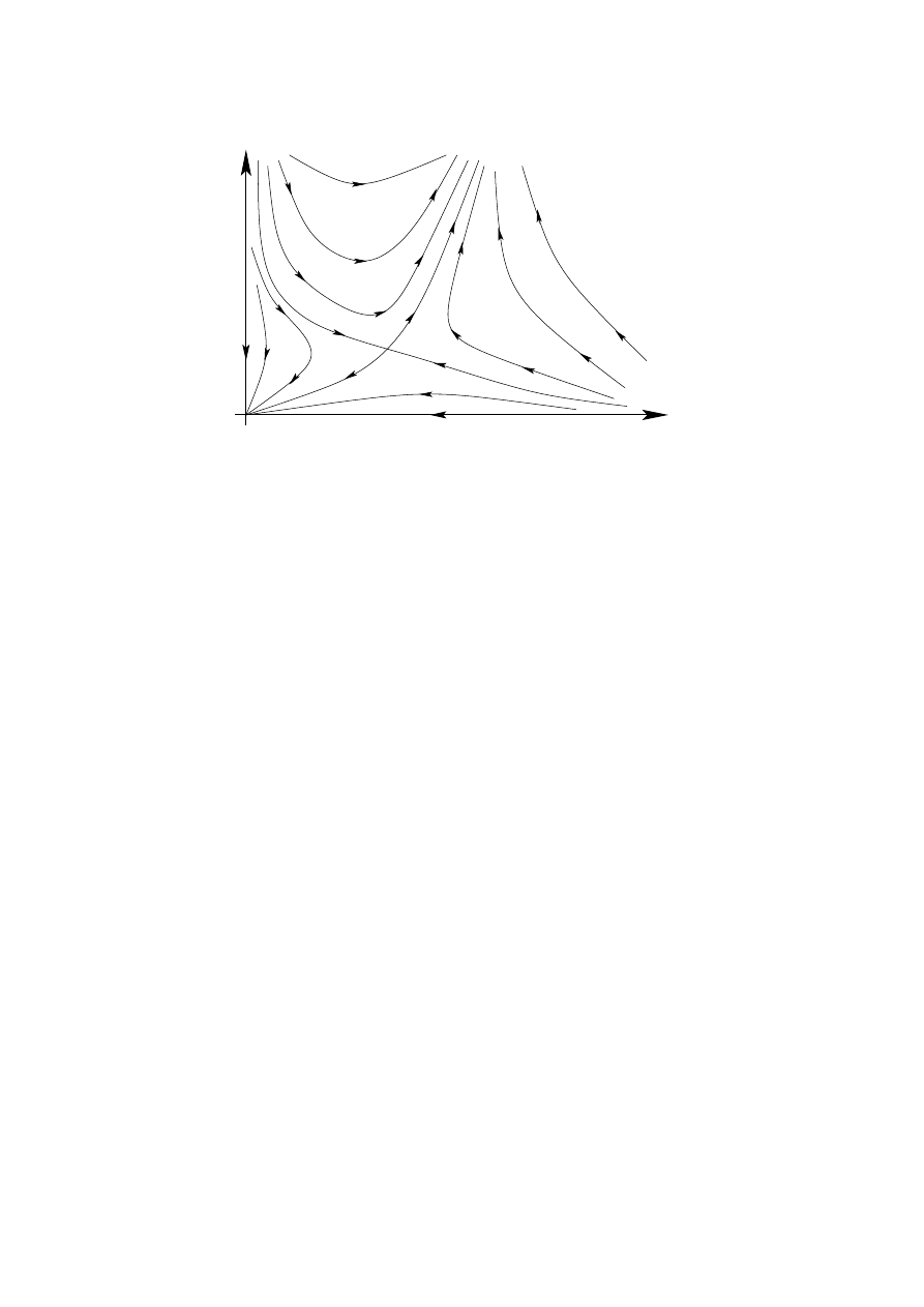
λ
λ
2
1
F
O
Fig. 17: Example of a renormalization group flow.
Therefore we can picture the action of the renormalization group transformation as a flow in
the space of coupling constants. In Fig. 17 we have depicted an example of such a flow in the case
of a system with two coupling constants
λ
1
and
λ
2
. In this example we find two fixed points, one at
the origin
O and another at F for a finite value of the couplings. The arrows indicate the direction
in which the renormalization group flow acts. The free theory at
λ
1
= λ
2
= 0 is a stable fix point
since any perturbation
δλ
1
, δλ
2
> 0 makes the theory flow back to the free theory at long distances.
On the other hand, the fixed point
F is stable with respect to certain type of perturbations (along the
line with incoming arrows) whereas for any other perturbations the system flows either to the free
theory at the origin or to a theory with infinite values for the couplings.
Quantum field theory. Let us see now how these ideas of the renormalization group apply to
Field Theory. Let us begin with a quantum field theory defined by the Lagrangian
L[φ
a
] =
L
0
[φ
a
] +
X
i
g
i
O
i
[φ
a
],
(8.49)
where
L
0
[φ
a
] is the kinetic part of the Lagrangian and g
i
are the coupling constants associated
with the operators
O
i
[φ
a
]. In order to make sense of the quantum theory we introduce a cutoff in
momenta
Λ. In principle we include all operators
O
i
compatible with the symmetries of the theory.
In section 8.2 we saw how in the cases of QED and QCD, the value of the coupling constant
changed with the scale from its value at the scale
Λ. We can understand now this behavior along the
lines of the analysis presented above for the Ising model. If we would like to compute the effective
dynamics of the theory at an energy scale
µ < Λ we only have to integrate out all physical models
with energies between the cutoff
Λ and the scale of interest µ. This is analogous to what we did in
the Ising model by replacing the original spins by the block spins. In the case of field theory the
94

effective action
S[φ
a
, µ] at scale µ can be written in the language of functional integration as
e
iS
[φ
′
a
,µ
]
=
Z
µ<p<
Λ
Y
a
Dφ
a
e
iS
[φ
a
,
Λ]
.
(8.50)
Here
S[φ
a
, Λ] is the action at the cutoff scale
S[φ
a
, Λ] =
Z
d
4
x
(
L
0
[φ
a
] +
X
i
g
i
(Λ)
O
i
[φ
a
]
)
(8.51)
and the functional integral in Eq. (8.50) is carried out only over the field modes with momenta in
the range
µ < p < Λ. The action resulting from integrating out the physics at the intermediate
scales between
Λ and µ depends not on the original field variable φ
a
but on some renormalized
field
φ
′
a
. At the same time the couplings
g
i
(µ) differ from their values at the cutoff scale g
i
(Λ).
This is analogous to what we learned in the Ising model: by integrating out short distance physics
we ended up with a new Hamiltonian depending on renormalized effective spin variables and with
renormalized values for the coupling constants. Therefore the resulting effective action at scale
µ
can be written as
S[φ
′
a
, µ] =
Z
d
4
x
(
L
0
[φ
′
a
] +
X
i
g
i
(µ)
O
i
[φ
′
a
]
)
.
(8.52)
This Wilsonian interpretation of renormalization sheds light to what in section 8.1 might have
looked just a smart way to get rid of the infinities. The running of the coupling constant with
the energy scale can be understood now as a way of incorporating into an effective action at scale
µ
the effects of field excitations at higher energies
E > µ.
As in statistical mechanics there are also quantum field theories that are fixed points of the
renormalization group flow, i.e. whose coupling constants do not change with the scale. We have
encountered them already in Section 8.2 when studying the properties of the beta function. The
most trivial example of such theories are massless free quantum field theories, but there are also
examples of four-dimensional interacting quantum field theories which are scale invariant. Again
we can ask the question of what happens when a scale invariant theory is perturbed with some
operator. In general the perturbed theory is not scale invariant anymore but we may wonder whether
the perturbed theory flows at low energies towards or away the theory at the fixed point.
In quantum field theory this can be decided by looking at the canonical dimension
d[
O] of the
operator
O[φ
a
] used to perturb the theory at the fixed point. In four dimensions the three possibilities
are defined by:
–
d[
O] > 4: irrelevant perturbation. The running of the coupling constants takes the theory
back to the fixed point.
–
d[
O] < 4: relevant perturbation. At low energies the theory flows away from the scale-
invariant theory.
–
d[
O] = 4: marginal deformation. The direction of the flow cannot be decided only on dimen-
sional grounds.
95

As an example, let us consider first a massless fermion theory perturbed by a four-fermion
interaction term
L = iψ∂/ψ −
1
M
2
(ψψ)
2
.
(8.53)
This is indeed a perturbation by an irrelevant operator, since in four-dimensions
[ψ] =
3
2
. Inter-
actions generated by the extra term are suppressed at low energies since typically their effects are
weighted by the dimensionless factor
E
2
M
2
, where
E is the energy scale of the process. This means
that as we try to capture the relevant physics at lower and lower energies the effect of the pertur-
bation is weaker and weaker rendering in the infrared limit
E
→ 0 again a free theory. Hence, the
irrelevant perturbation in (8.53) makes the theory flow back to the fixed point.
On the other hand relevant operators dominate the physics at low energies. This is the case,
for example, of a mass term. As we lower the energy the mass becomes more important and once
the energy goes below the mass of the field its dynamics is completely dominated by the mass term.
This is, for example, how Fermi’s theory of weak interactions emerges from the Standard Model at
energies below the mass of the
W
±
boson
2
u
e
+
d
W
+
ν
e
=
⇒
3
u
e
+
d
ν
e
At energies below
M
W
= 80.4 GeV the dynamics of the W
+
boson is dominated by its mass term
and therefore becomes nonpropagating, giving rise to the effective four-fermion Fermi theory.
To summarize our discussion so far, we found that while relevant operators dominate the dy-
namics in the infrared, taking the theory away from the fixed point, irrelevant perturbations become
suppressed in the same limit. Finally we consider the effect of marginal operators. As an example
we take the interaction term in massless QED,
O = ψγ
µ
ψ A
µ
. Taking into account that in
d = 4 the
dimension of the electromagnetic potential is
[A
µ
] = 1 the operator
O is a marginal perturbation.
In order to decide whether the fixed point theory
L
0
=
−
1
4
F
µν
F
µν
+ iψD
/ ψ
(8.54)
is restored at low energies or not we need to study the perturbed theory in more detail. This we have
done in section 8.1 where we learned that the effective coupling in QED decreases at low energies.
Then we conclude that the perturbed theory flows towards the fixed point in the infrared.
As an example of a marginal operator with the opposite behavior we can write the Lagrangian
for a SU(
N
c
) gauge theory,
L = −
1
4
F
a
µν
F
a µν
, as
L = −
1
4
∂
µ
A
a
ν
− ∂
ν
A
a
µ
(∂
µ
A
a ν
− ∂
ν
A
a µ
)
− 4gf
abc
A
a
µ
A
b
ν
∂
µ
A
c ν
+ g
2
f
abc
f
ade
A
b
µ
A
c
ν
A
d µ
A
e ν
≡ L
0
+
O
g
,
(8.55)
96
i.e. a marginal perturbation of the free theory described by
L
0
, which is obviously a fixed point
under renormalization group transformations. Unlike the case of QED we know that the full theory
is asymptotically free, so the coupling constant grows at low energies. This implies that the operator
O
g
becomes more and more important in the infrared and therefore the theory flows away the fixed
point in this limit.
It is very important to notice here that in the Wilsonian view the cutoff is not necessarily
regarded as just some artifact to remove infinities but actually has a physical origin. For example in
the case of Fermi’s theory of
β-decay there is a natural cutoff Λ = M
W
at which the theory has to
be replaced by the Standard Model. In the case of the Standard Model itself the cutoff can be taken
at Planck scale
Λ
≃ 10
19
GeV or the Grand Unification scale
Λ
≃ 10
16
GeV, where new degrees
of freedom are expected to become relevant. The cutoff serves the purpose of cloaking the range of
energies at which new physics has to be taken into account.
Provided that in the Wilsonian approach the quantum theory is always defined with a physical
cutoff, there is no fundamental difference between renormalizable and nonrenormalizable theories.
Actually, a renormalizable field theory, like the Standard Model, can generate nonrenormalizable
operators at low energies such as the effective four-fermion interaction of Fermi’s theory. They
are not sources of any trouble if we are interested in the physics at scales much below the cutoff,
E
≪ Λ, since their contribution to the amplitudes will be suppressed by powers of
E
Λ
.
9
Special topics
9.1
Creation of particles by classical fields
Particle creation by a classical source. In a free quantum field theory the total number of particles
contained in a given state of the field is a conserved quantity. For example, in the case of the quantum
scalar field studied in section 3 we have that the number operator commutes with the Hamiltonian
b
n
≡
Z
d
3
k
(2π)
3
α
†
(~k)α(~k),
[ b
H, bn] = 0.
(9.1)
This means that any states with a well-defined number of particle excitations will preserve this
number at all times. The situation, however, changes as soon as interactions are introduced, since in
this case particles can be created and/or destroyed as a result of the dynamics.
Another case in which the number of particles might change is if the quantum theory is cou-
pled to a classical source. The archetypical example of such a situation is the Schwinger effect,
in which a classical strong electric field produces the creation of electron-positron pairs out of the
vacuum. However, before plunging into this more involved situation we can illustrate the relevant
physics involved in the creation of particles by classical sources with the help of the simplest ex-
ample: a free scalar field theory coupled to a classical external source
J(x). The action for such a
theory can be written as
S =
Z
d
4
x
1
2
∂
µ
φ(x)∂
µ
φ(x)
−
m
2
2
φ(x)
2
+ J(x)φ(x)
,
(9.2)
where
J(x) is a real function of the coordinates. Its identification with a classical source is obvious
97
once we calculate the equations of motion
∇
2
+ m
2
φ(x) = J(x).
(9.3)
Our plan is to quantize this theory but, unlike the case analyzed in section 3, now the presence of
the source
J(x) makes the situation a bit more involved. The general solution to the equations of
motion can be written in terms of the retarded Green function for the Klein-Gordon equation as
φ(x) = φ
0
(x) + i
Z
d
4
x
′
G
R
(x
− x
′
)J(x
′
),
(9.4)
where
φ
0
(x) is a general solution to the homogeneous equation and
G
R
(t, ~x) =
Z
d
4
k
(2π)
4
i
k
2
− m
2
e
−ik·x
= i θ(t)
Z
d
3
k
(2π)
3
1
2ω
k
e
−iω
k
t
+~k·~x
− e
iω
k
t
−i~p·~x
,
(9.5)
with
θ(x) the Heaviside step function. The integration contour to evaluate the integral over p
0
surrounds the poles at
p
0
=
±ω
k
from above. Since
G
R
(t, ~x) = 0 for t < 0, the function φ
0
(x)
corresponds to the solution of the field equation at
t
→ −∞, before the interaction with the external
source
21
To make the argument simpler we assume that
J(x) is switched on at t = 0, and only last for
a time
τ , that is
J(t, ~x) = 0
if
t < 0 or t > τ .
(9.6)
We are interested in a solution of (9.3) for times after the external source has been switched off,
t > τ . In this case the expression (9.5) can be written in terms of the Fourier modes e
J(ω, ~k) of the
source as
φ(t, ~x) = φ
0
(x) + i
Z
d
3
k
(2π)
3
1
2ω
k
h
e
J(ω
k
, ~k)e
−iω
k
t
+i~k·~x
− e
J(ω
k
, ~k)
∗
e
iω
k
t
−i~k·~x
i
.
(9.7)
On the other hand, the general solution
φ
0
(x) has been already computed in Eq. (3.53). Combining
this result with Eq. (9.7) we find the following expression for the late time general solution to the
Klein-Gordon equation in the presence of the source
φ(t, x) =
Z
d
3
k
(2π)
3
1
√
2ω
k
α(~k) +
i
√
2ω
k
e
J(ω
k
, ~k)
e
−iω
k
t
+i~k·~x
+
α
∗
(~k)
−
i
√
2ω
k
e
J (ω
k
, ~k)
∗
e
iω
k
t
−i~k·~x
.
(9.8)
We should not forget that this is a solution valid for times
t > τ , i.e. once the external source has
been disconnected. On the other hand, for
t < 0 we find from Eqs. (9.4) and (9.5) that the general
solution is given by Eq. (3.53).
21
We could have taken instead the advanced propagator G
A
(x) in which case φ
0
(x) would correspond to the solution
to the equation at large times, after the interaction with J
(x).
98
Now we can proceed to quantize the theory. The conjugate momentum
π(x) = ∂
0
φ(x) can
be computed from Eqs. (3.53) and (9.8). Imposing the canonical equal time commutation relations
(3.50) we find that
α(~k), α
†
(~k) satisfy the creation-annihilation algebra (3.27). From our previous
calculation we find that for
t > τ the expansion of the operator φ(x) in terms of the creation-
annihilation operators
α(~k), α
†
(~k) can be obtained from the one for t < 0 by the replacement
α(~k)
−→ β(~k) ≡ α(~k) +
i
√
2ω
k
e
J(ω
k
, ~k),
α
†
(~k)
−→ β
†
(~k)
≡ α
†
(~k)
−
i
√
2ω
k
e
J (ω
k
, ~k)
∗
.
(9.9)
Actually, since e
J (ω
k
, ~k) is a c-number, the operators β(~k), β
†
(~k) satisfy the same algebra as α(~k),
α
†
(~k) and therefore can be interpreted as well as a set of creation-annihilation operators. This means
that we can define two vacuum states,
|0
−
i, |0
+
i associated with both sets of operators
α(~k)
|0
−
i = 0
β(~k)
|0
+
i = 0
∀ ~k.
(9.10)
For an observer at
t < 0, α(~k) and α(~k) are the natural set of creation-annihilation operators
in terms of which to expand the field operator
φ(x). After the usual zero-point energy subtraction
the Hamiltonian is given by
b
H
(−)
=
Z
d
3
k ω
k
α
†
(~k)α(~k)
(9.11)
and the ground state of the spectrum for this observer is the vacuum
|0
−
i. At the same time, a
second observer at
t > τ will also see a free scalar quantum field (the source has been switched
off at
t = τ ) and consequently will expand φ in terms of the second set of creation-annihilation
operators
β(~k), β
†
(~k). In terms of this operators the Hamiltonian is written as
b
H
(+)
=
Z
d
3
k ω
k
β
†
(~k)β(~k).
(9.12)
Then for this late-time observer the ground state of the Hamiltonian is the second vacuum state
|0
+
i.
In our analysis we have been working in the Heisenberg picture, where states are time-
independent and the time dependence comes in the operators. Therefore the states of the theory
are globally defined. Suppose now that the system is in the “in” ground state
|0
−
i. An observer at
t < 0 will find that there are no particles
bn
(−)
|0
−
i = 0.
(9.13)
However the late-time observer will find that the state
|0
−
i contains an average number of particles
given by
h0
−
|bn
(+)
|0
−
i =
Z
d
3
k
(2π)
3
1
2ω
k
e
J(ω
k
, ~k)
2
.
(9.14)
99
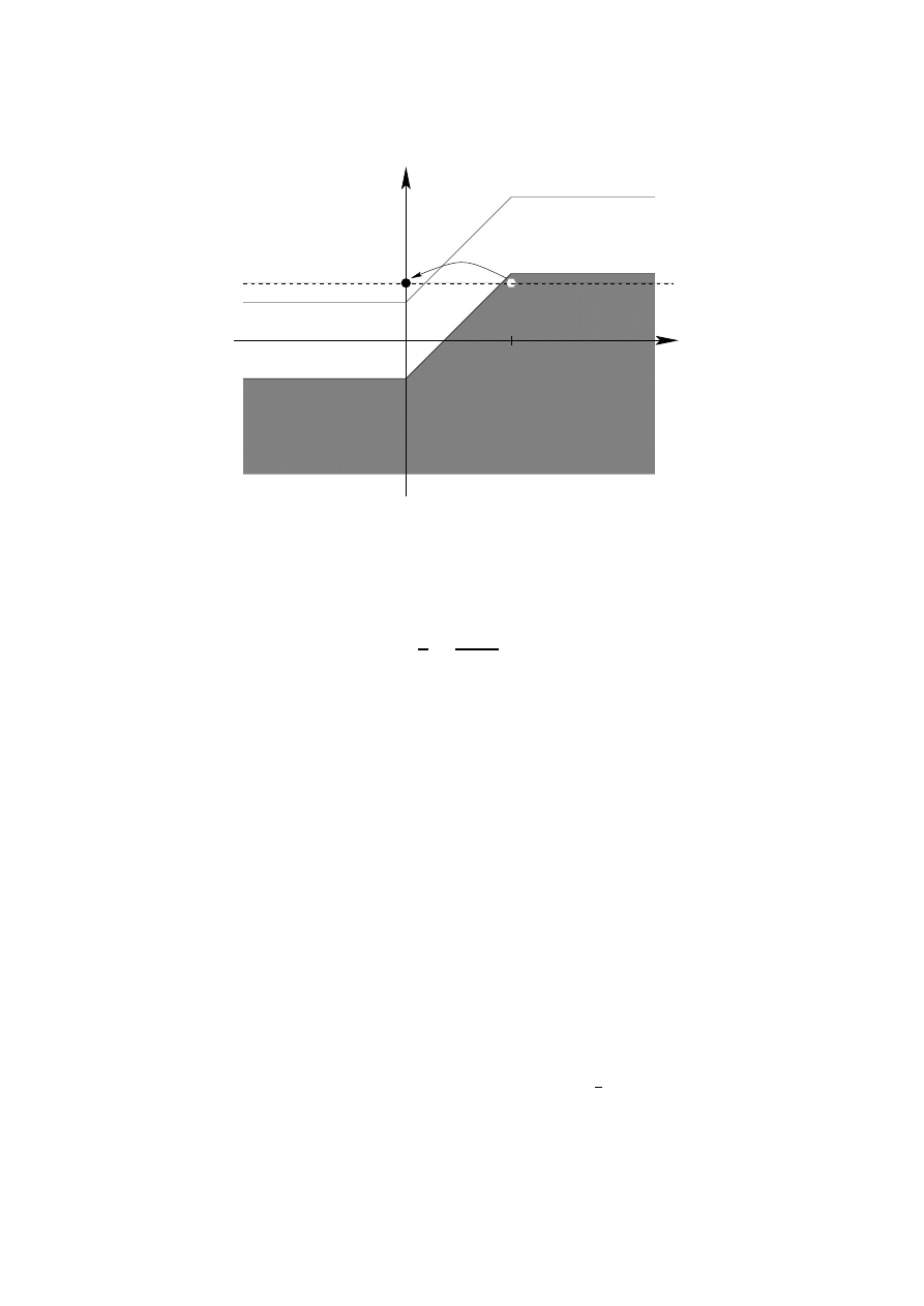
E
x
e +
0
Dirac sea
e −
−m
m
E
0
L
Fig. 18: Pair creation by a electric field in the Dirac sea picture.
Moreover,
|0
−
i is no longer the ground state for the “out” observer. On the contrary, this state have
a vacuum expectation value for b
H
(+)
h0
−
| b
H
(+)
|0
−
i =
1
2
Z
d
3
k
(2π)
3
˜
J(ω
k
, ~k)
2
.
(9.15)
The key to understand what is going on here lies in the fact that the external source breaks
the invariance of the theory under space-time translations. In the particular case we have studied
here where
J(x) has support over a finite time interval 0 < t < τ , this implies that the vacuum is
not invariant under time translations, so observers at different times will make different choices of
vacuum that will not necessarily agree with each other. This is clear in our example. An observer in
t < τ will choose the vacuum to be the lowest energy state of her Hamiltonian,
|0
−
i. On the other
hand, the second observer at late times
t > τ will naturally choose
|0
+
i as the vacuum. However,
for this second observer, the state
|0
−
i is not the vacuum of his Hamiltonian, but actually an excited
state that is a superposition of states with well-defined number of particles. In this sense it can be
said that the external source has the effect of creating particles out of the “in” vacuum. Besides,
this breaking of time translation invariance produces a violation in the energy conservation as we
see from Eq. (9.15). Particles are actually created from the energy pumped into the system by the
external source.
The Schwinger effect. A classical example of creation of particles by a external field was
pointed out by Schwinger [43] and consists of the creation of electron-positron pairs by a strong
electric field. In order to illustrate this effect we are going to follow a heuristic argument based on
the Dirac sea picture and the WKB approximation.
In the absence of an electric field the vacuum state of a spin-
1
2
field is constructed by filling
all the negative energy states as depicted in Fig. 2. Let us now connect a constant electric field
100
~
E = −E~u
x
in the range
0 < x < L created by a electrostatic potential
V (~r) =
0
x < 0
E(x − x
0
)
0 < x < L
EL
x > L
(9.16)
After the field has been switched on, the Dirac sea looks like in Fig. 18. In particular we find that
if
EL > 2m there are negative energy states at x > L with the same energy as the positive energy
states in the region
x < 0. Therefore it is possible for an electron filling a negative energy state
with energy close to
−2m to tunnel through the forbidden region into a positive energy state. The
interpretation of such a process is the production of an electron-positron pair out of the electric field.
We can compute the rate at which such pairs are produced by using the WKB approximation.
Focusing for simplicity on an electron on top of the Fermi surface near
x = L with energy E
0
, the
transmission coefficient in this approximation is given by
22
T
WKB
= exp
"
−2
Z
1
e
E
E
0
+
√
m
2
+~
p
2
T
1
e
E
E
0
−
√
m
2
+~
p
2
T
dx
q
m
2
− [E
0
− eE(x − x
0
)]
2
+ ~p
2
T
#
= exp
h
−
π
e
E
~p
2
T
+ m
2
i
,
(9.17)
where
p
2
T
≡ p
2
y
+ p
2
z
. This gives the transition probability per unit time and per unit cross section
dydz for an electron in the Dirac sea with transverse momentum ~p
T
and energy
E
0
. To get the total
probability per unit time and per unit volume we have to integrate over all possible values of
~p
T
and
E
0
. Actually, in the case of the energy, because of the relation between
E
0
and the coordinate
x at
which the particle penetrates into the barrier we can write
dE
0
2π
=
e
E
2π
dx and the total probability per
unit time and per unit volume for the creation of a pair is given by
W = 2
e
E
2π
Z
d
2
p
T
(2π)
2
e
−
π
e
E
(
~
p
2
T
+m
2
) = e
2
E
2
4π
3
e
−
π m2
e
E
,
(9.18)
where the factor of
2 accounts for the two polarizations of the electron.
Then production of electron-positron pairs is exponentially suppressed and it is only sizeable
for strong electric fields. To estimate its order of magnitude it is useful to restore the powers of
c
and ~ in (9.18)
W =
e
2
E
2
4π
3
c~
2
e
−
π m2c3
~
e
E
(9.19)
The exponential suppression of the pair production disappears when the electric field reaches the
critical value
E
crit
at which the exponent is of order one
E
crit
=
m
2
c
3
~
e
≃ 1.3 × 10
16
V cm
−1
.
(9.20)
22
Notice that the electron satisfy the relativistic dispersion relation E
=
p
~
p
2
+ m
2
+ V and therefore
−p
2
x
=
m
2
− (E − V )
2
+ ~
p
2
T
. The integration limits are set by those values of x at which p
x
= 0.
101
This is indeed a very strong field which is extremely difficult to produce. A similar effect, however,
takes place also in a time-varying electric field [44] and there is the hope that pair production could
be observed in the presence of the alternating electric field produced by a laser.
The heuristic derivation that we followed here can be made more precise in QED. There the
decay of the vacuum into electron-positron pairs can be computed from the imaginary part of the
effective action
Γ[A
µ
] in the presence of a classical gauge potential A
µ
iΓ[A
µ
]
≡
4
+
5
+
6
+ . . .
= log det
1
− ie/
A
1
i∂/
− m
.
(9.21)
This determinant can be computed using the standard heat kernel techniques. The probability of
pair production is proportional to the imaginary part of
iΓ[A
µ
] and gives
W =
e
2
E
2
4π
3
∞
X
n
=1
1
n
2
e
−n
π m2
e
E
.
(9.22)
Our simple argument based on tunneling in the Dirac sea gave only the leading term of Schwinger’s
result (9.22). The remaining terms can be also captured in the WKB approximation by taking into
account the probability of production of several pairs, i.e. the tunneling of more than one electron
through the barrier.
Here we have illustrated the creation of particles by semiclassical sources in Quantum Field
Theory using simple examples. Nevertheless, what we learned has important applications to the
study of quantum fields in curved backgrounds. In Quantum Field Theory in Minkowski space-time
the vacuum state is invariant under the Poincar´e group and this, together with the covariance of
the theory under Lorentz transformations, implies that all inertial observers agree on the number of
particles contained in a quantum state. The breaking of such invariance, as happened in the case of
coupling to a time-varying source analyzed above, implies that it is not possible anymore to define
a state which would be recognized as the vacuum by all observers.
This is precisely the situation when fields are quantized on curved backgrounds. In particular,
if the background is time-dependent (as it happens in a cosmological setup or for a collapsing star)
different observers will identify different vacuum states. As a consequence what one observer call
the vacuum will be full of particles for a different observer. This is precisely what is behind the
phenomenon of Hawking radiation [45]. The emission of particles by a physical black hole formed
from gravitational collapse of a star is the consequence of the fact that the vacuum state in the
asymptotic past contain particles for an observer in the asymptotic future. As a consequence, a
detector located far away from the black hole detects a stream of thermal radiation with temperature
T
Hawking
=
~
c
3
8πG
N
k M
(9.23)
102
where
M is the mass of the black hole, G
N
is Newton’s constant and
k is Boltzmann’s constant.
There are several ways in which this results can be obtained. A more heuristic way is perhaps to
think of this particle creation as resulting from quantum tunneling of particles across the potential
barrier posed by gravity [46].
9.2
Supersymmetry
One of the things that we have learned in our journey around the landscape of Quantum Field
Theory is that our knowledge of the fundamental interactions in Nature is based on the idea of
symmetry, and in particular gauge symmetry. The Lagrangian of the Standard Model can be written
just including all possible renormalizable terms (i.e. with canonical dimension smaller o equal to 4)
compatible with the gauge symmetry SU(3)
×SU(2)×U(1) and Poincar´e invariance. All attempts to
go beyond start with the question of how to extend the symmetries of the Standard Model.
As explained in Section 5.1, in a quantum field theoretical description of the interaction of
elementary particles the basic observable quantity to compute is the scattering or
S-matrix giving the
probability amplitude for the scattering of a number of incoming particles with a certain momentum
into some final products
A(in −→ out) = h~p
1
′
, . . . ; out
|~p
1
, . . . ; in
i.
(9.24)
An explicit symmetry of the theory has to be necessarily a symmetry of the
S-matrix. Hence it is
fair to ask what is the largest symmetry of the
S-matrix.
Let us ask this question in the simple case of the scattering of two particles with four-momenta
p
1
and
p
2
in the
t-channel
7
p
1
p
2
p
′
1
p
′
2
We will make the usual assumptions regarding positivity of the energy and analyticity. Invariance
of the theory under the Poincar´e group implies that the amplitude can only depend on the scattering
angle
ϑ through
t = (p
′
1
− p
1
)
2
= 2 m
2
1
− p
1
· p
′
1
= 2 m
2
1
− E
1
E
′
1
+
|~p
1
||~p
1
′
| cos ϑ
.
(9.25)
If there would be any extra bosonic symmetry of the theory it would restrict the scattering angle to a
set of discrete values. In this case the
S-matrix cannot be analytic since it would vanish everywhere
except for the discrete values selected by the extra symmetry.
Actually, the only way to extend the symmetry of the theory without renouncing to the ana-
lyticity of the scattering amplitudes is to introduce “fermionic” symmetries, i.e. symmetries whose
generators are anticommuting objects [47]. This means that in addition to the generators of the
Poincar´e group
23
P
µ
,
M
µν
and the ones for the internal gauge symmetries
G, we can introduce a
23
The generators M
µν
are related with the ones for boost and rotations introduced in section 4.1 by J
i
≡ M
0
i
,
M
i
=
1
2
ε
ijk
M
jk
. In this section we also use the “dotted spinor” notation, in which spinors in the
(
1
2
, 0
) and (0,
1
2
)
representations of the Lorentz group are indicated respectively by undotted (a, b, . . .) and dotted (
˙a, ˙b, . . .) indices.
103
number of fermionic generators
Q
I
a
,
Q
˙a I
(
I = 1, . . . ,
N ), where Q
˙a I
= (Q
I
a
)
†
. The most general
algebra that these generators satisfy is the
N -extended supersymmetry algebra [48]
{Q
I
a
, Q
˙b J
} = 2σ
µ
a˙b
P
µ
δ
I
J
,
{Q
I
a
, Q
J
b
} = 2ε
ab
Z
IJ
,
(9.26)
{Q
I
˙a
, Q
J
˙b
} = −2ε
˙a˙b
Z
IJ
,
(9.27)
where
Z
IJ
∈ C commute with any other generator and satisfies Z
IJ
=
−Z
J I
. Besides we have the
commutators that determine the Poincar´e transformations of the fermionic generators
Q
I
a
,
Q
˙a J
[Q
I
a
, P
µ
] = [Q
˙a I
, P
µ
] = 0,
[Q
I
a
, M
µν
] =
1
2
(σ
µν
)
b
a
Q
I
b
,
(9.28)
[Q
a I
, M
µν
] =
−
1
2
(σ
µν
)
˙b
˙a
Q
˙b I
,
where
σ
0i
=
−iσ
i
,
σ
ij
= ε
ijk
σ
k
and
σ
µν
= (σ
µν
)
†
. These identities simply mean that
Q
I
a
,
Q
˙a J
transform respectively in the
(
1
2
, 0) and (0,
1
2
) representations of the Lorentz group.
We know that the presence of a global symmetry in a theory implies that the spectrum can be
classified in multiplets with respect to that symmetry. In the case of supersymmetry start with the
case case
N = 1 in which there is a single pair of supercharges Q
a
,
Q
˙a
satisfying the algebra
{Q
a
, Q
˙b
} = 2σ
µ
a˙b
P
µ
,
{Q
a
, Q
b
} = {Q
˙a
, Q
˙b
} = 0.
(9.29)
Notice that in the
N = 1 case there is no possibility of having central charges.
We study now the representations of the supersymmetry algebra (9.29), starting with the mass-
less case. Given a state
|ki satisfying k
2
= 0, we can always find a reference frame where the
four-vector
k
µ
takes the form
k
µ
= (E, 0, 0, E). Since the theory is Lorentz covariant we can obtain
the representation of the supersymmetry algebra in this frame where the expressions are simpler. In
particular, the right-hand side of the first anticommutator in Eq. (9.29) is given by
2σ
µ
a˙b
P
µ
= 2(P
0
− σ
3
P
3
) =
0
0
0 4E
.
(9.30)
Therefore the algebra of supercharges in the massless case reduces to
{Q
1
, Q
†
1
} = {Q
1
, Q
†
2
} = 0,
{Q
2
, Q
†
2
} = 4E.
(9.31)
The commutator
{Q
1
, Q
†
1
} = 0 implies that the action of Q
1
on any state gives a zero-norm state of
the Hilbert space
||Q
1
|Ψi|| = 0. If we want the theory to preserve unitarity we must eliminate these
null states from the spectrum. This is equivalent to setting
Q
1
≡ 0. On the other hand, in terms of
the second generator
Q
2
we can define the operators
a =
1
2
√
E
Q
2
,
a
†
=
1
2
√
E
Q
†
2
,
(9.32)
104
which satisfy the algebra of a pair of fermionic creation-annihilation operators,
{a, a
†
} = 1, a
2
=
(a
†
)
2
= 0. Starting with a vacuum state a
|λi = 0 with helicity λ we can build the massless multiplet
|λi,
|λ +
1
2
i ≡ a
†
|λi.
(9.33)
Here we consider two important cases:
– Scalar multiplet: we take the vacuum state to have zero helicity
|0
+
i so the multiplet consists
of a scalar and a helicity-
1
2
state
|0
+
i,
|
1
2
i ≡ a
†
|0
+
i.
(9.34)
However, this multiplet is not invariant under the CPT transformation which reverses the sign
of the helicity of the states. In order to have a CPT-invariant theory we have to add to this
multiplet its CPT-conjugate which can be obtain from a vacuum state with helicity
λ =
−
1
2
|0
−
i,
| −
1
2
i.
(9.35)
Putting them together we can combine the two zero helicity states with the two fermionic
ones into the degrees of freedom of a complex scalar field and a Weyl (or Majorana) spinor.
– Vector multiplet: now we take the vacuum state to have helicity
λ =
1
2
, so the multiplet
contains also a massless state with helicity
λ = 1
|
1
2
i,
|1i ≡ a
†
|
1
2
i.
(9.36)
As with the scalar multiplet we add the CPT conjugated obtained from a vacuum state with
helicity
λ =
−1
| −
1
2
i,
| − 1i,
(9.37)
which together with (9.36) give the propagating states of a gauge field and a spin-
1
2
gaugino.
In both cases we see the trademark of supersymmetric theories: the number of bosonic and fermionic
states within a multiplet are the same.
In the case of extended supersymmetry we have to repeat the previous analysis for each su-
persymmetry charge. At the end, we have
N sets of fermionic creation-annihilation operators
{a
I
, a
†
I
} = δ
I
J
,
(a
I
)
2
= (a
†
I
)
2
= 0. Let us work out the case of
N = 8 supersymmetry. Since
for several reasons we do not want to have states with helicity larger than
2, we start with a vacuum
state
| − 2i of helicity λ = −2. The rest of the states of the supermultiplet are obtained by applying
105
the eight different creation operators
a
†
I
to the vacuum:
λ = 2 :
a
†
1
. . . a
†
8
| − 2i
8
8
= 1 state,
λ =
3
2
:
a
†
I
1
. . . a
†
I
7
| − 2i
8
7
= 8 states,
λ = 1 :
a
†
I
1
. . . a
†
I
6
| − 2i
8
6
= 28 states,
λ =
1
2
:
a
†
I
1
. . . a
†
I
5
| − 2i
8
5
= 56 states,
λ = 0 :
a
†
I
1
. . . a
†
I
4
| − 2i
8
4
= 70 states,
(9.38)
λ =
−
1
2
:
a
†
I
1
a
†
I
2
a
†
I
3
| − 2i
8
3
= 56 states,
λ =
−1 :
a
†
I
1
a
†
I
2
| − 2i
8
2
= 28 states,
λ =
−
3
2
:
a
†
I
1
| − 2i
8
1
= 8 states,
λ =
−2 :
| − 2i
1 state
.
Putting together the states with opposite helicity we find that the theory contains:
– 1 spin-2 field
g
µν
(a graviton),
– 8 spin-
3
2
gravitino fields
ψ
I
µ
,
– 28 gauge fields
A
[IJ]
µ
,
– 56 spin-
1
2
fermions
ψ
[IJK]
,
– 70 scalars
φ
[IJKL]
,
where by
[IJ...] we have denoted that the indices are antisymmetrized. We see that, unlike the
massless multiplets of
N = 1 supersymmetry studied above, this multiplet is CPT invariant by
itself. As in the case of the massless
N = 1 multiplet, here we also find as many bosonic as
fermionic states:
bosons:
1 + 28 + 70 + 28 + 1 = 128 states,
fermions:
8 + 56 + 56 + 8 = 128 states.
Now we study briefly the case of massive representations
|ki, k
2
= M
2
. Things become
simpler if we work in the rest frame where
P
0
= M and the spatial components of the momentum
vanish. Then, the supersymmetry algebra becomes:
{Q
I
α
, Q
˙
β J
} = 2Mδ
α ˙
β
δ
I
J
.
(9.39)
106
We proceed now in a similar way to the massless case by defining the operators
a
I
α
≡
1
√
2M
Q
I
α
,
a
†
˙
α I
≡
1
√
2M
Q
˙
α I
.
(9.40)
The multiplets are found by choosing a vacuum state with a definite spin. For example, for
N = 1
and taking a spin-0 vacuum
|0i we find three states in the multiplet transforming irreducibly with
respect to the Lorentz group:
|0i,
a
†
˙
α
|0i,
ε
˙
α ˙
β
a
†
˙
α
a
†
˙
β
|0i,
(9.41)
which, once transformed back from the rest frame, correspond to the physical states of two spin-0
bosons and one spin-
1
2
fermion. For
N -extended supersymmetry the corresponding multiplets can
be worked out in a similar way.
The equality between bosonic and fermionic degrees of freedom is at the root of many of
the interesting properties of supersymmetric theories. For example, in section 4 we computed the
divergent vacuum energy contributions for each real bosonic or fermionic propagating degree of
freedom is
24
E
vac
=
±
1
2
δ(~0)
Z
d
3
p ω
p
,
(9.42)
where the sign
± corresponds respectively to bosons and fermions. Hence, for a supersymmet-
ric theory the vacuum energy contribution exactly cancels between bosons and fermions. This
boson-fermion degeneracy is also responsible for supersymmetric quantum field theories being less
divergent than nonsupersymmetric ones.
Appendix: A crash course in Group Theory
In this Appendix we summarize some basic facts about Group Theory. Given a group
G a represen-
tation of
G is a correspondence between the elements of G and the set of linear operators acting on
a vector space
V , such that for each element of the group g
∈ G there is a linear operator D(g)
D(g) : V
−→ V
(A.43)
satisfying the group operations
D(g
1
)D(g
2
) = D(g
1
g
2
),
D(g
−1
1
) = D(g
1
)
−1
,
g
1
, g
2
∈ G.
(A.44)
The representation
D(g) is irreducible if and only if the only operators A : V
→ V commuting with
all the elements of the representation
D(g) are the ones proportional to the identity
[D(g), A] = 0,
∀g
⇐⇒
A = λ1,
λ
∈ C
(A.45)
24
For a boson, this can be read off Eq. (3.56). In the case of fermions, the result of Eq. (4.44) gives the vacuum
energy contribution of the four real propagating degrees of freedom of a Dirac spinor.
107

More intuitively, we can say that a representation is irreducible if there is no proper subspace
U
⊂ V
(i.e.
U
6= V and U 6= ∅) such that D(g)U ⊂ U for every element g ∈ G.
Here we are specially interested in Lie groups whose elements are labelled by a number of
continuous parameters. In mathematical terms this means that a Lie group is a manifold
M together
with an operation
M × M −→ M that we will call multiplication that satisfies the associativity
property
g
1
· (g
2
· g
3
) = (g
1
· g
2
)
· g
3
together with the existence of unity
g1 = 1g = g,for every
g
∈ M and inverse gg
−1
= g
−1
g = 1.
The simplest example of a Lie group is SO(2), the group of rotations in the plane. Each
element
R(θ) is labelled by the rotation angle θ, with the multiplication acting as R(θ
1
)R(θ
2
) =
R(θ
1
+θ
2
). Because the angle θ is defined only modulo 2π, the manifold of SO(2) is a circumference
S
1
.
One of the interesting properties of Lie groups is that in a neighborhood of the identity element
they can be expressed in terms of a set of generators
T
a
(
a = 1, . . . , dim G) as
D(g) = exp[
−iα
a
T
a
]
≡
∞
X
n
=0
(
−i)
n
n!
α
a
1
. . . α
a
n
T
a
1
. . . T
a
n
,
(A.46)
where
α
a
∈ C are a set of coordinates of M in a neighborhood of 1. Because of the general Baker-
Campbell-Haussdorf formula, the multiplication of two group elements is encoded in the value of
the commutator of two generators, that in general has the form
[T
a
, T
b
] = if
abc
T
c
,
(A.47)
where
f
abc
∈ C are called the structure constants. The set of generators with the commutator
operation form the Lie algebra associated with the Lie group. Hence, given a representation of the
Lie algebra of generators we can construct a representation of the group by exponentiation (at least
locally near the identity).
We illustrate these concept with some particular examples. For SU(2) each group element
is labelled by three real number
α
i
,
i = 1, 2, 3. We have two basic representations: one is the
fundamental representation (or spin
1
2
) defined by
D
1
2
(α
i
) = e
−
i
2
α
i
σ
i
,
(A.48)
with
σ
i
the Pauli matrices. The second one is the adjoint (or spin 1) representation which can be
written as
D
1
(α
i
) = e
−iα
i
J
i
,
(A.49)
where
J
1
=
0
0
0
0
0
1
0
−1 0
,
J
2
=
0 0
−1
0 0
0
1 0
0
,
J
3
=
0
1 0
−1 0 0
0
0 0
.
(A.50)
108
Actually,
J
i
(
i = 1, 2, 3) generate rotations around the x, y and z axis respectively. Representations
of spin
j
∈ N +
1
2
can be also constructed with dimension
dim D
j
(g) = 2j + 1.
(A.51)
As a second example we consider SU(3). This group has two basic three-dimensional repre-
sentations denoted by 3 and 3 which in QCD are associated with the transformation of quarks and
antiquarks under the color gauge symmetry SU(3). The elements of these representations can be
written as
D
3
(α
a
) = e
i
2
α
a
λ
a
,
D
3
(α
a
) = e
−
i
2
α
a
λ
T
a
(a = 1, . . . , 8),
(A.52)
where
λ
a
are the eight hermitian Gell-Mann matrices
λ
1
=
0 1 0
1 0 0
0 0 0
,
λ
2
=
0
−i 0
i
0
0
0
0
0
,
λ
3
=
1
0
0
0
−1 0
0
0
0
,
λ
4
=
0 0 1
0 0 0
1 0 0
,
λ
5
=
0 0
−i
0 0
0
i 0
0
,
λ
6
=
0 0 0
0 0 1
0 1 0
,
(A.53)
λ
7
=
0 0
0
0 0
−i
0 i
0
,
λ
8
=
1
√
3
0
0
0
1
√
3
0
0
0
−
2
√
3
.
Hence the generators of the representations 3 and 3 are given by
T
a
(3) =
1
2
λ
a
,
T
a
(3) =
−
1
2
λ
T
a
.
(A.54)
Irreducible representations can be classified in three groups: real, complex and pseudoreal.
– Real representations: a representation is said to be real if there is a symmetric matrix
S which
acts as intertwiner between the generators and their complex conjugates
T
a
=
−ST
a
S
−1
,
S
T
= S.
(A.55)
This is for example the case of the adjoint representation of SU(2) generated by the matrices
(A.50)
– Pseudoreal representations: are the ones for which an antisymmetric matrix
S exists with the
property
T
a
=
−ST
a
S
−1
,
S
T
=
−S.
(A.56)
As an example we can mention the spin-
1
2
representation of SU(2) generated by
1
2
σ
i
.
109

– Complex representations: finally, a representation is complex if the generators and their com-
plex conjugate are not related by a similarity transformation. This is for instance the case of
the two three-dimensional representations 3 and 3 of SU(3).
There are a number of invariants that can be constructed associated with an irreducible repre-
sentation
R of a Lie group G and that can be used to label such a representation. If T
a
R
are the gen-
erators in a certain representation
R of the Lie algebra, it is easy to see that the matrix
P
dim G
a
=1
T
a
R
T
a
R
commutes with every generator
T
a
R
. Therefore, because of Schur’s lemma, it has to be proportional
to the identity
25
. This defines the Casimir invariant
C
2
(R) as
dim G
X
a
=1
T
a
R
T
a
R
= C
2
(R)1.
(A.57)
A second invariant
T
2
(R) associated with a representation R can also be defined by the identity
Tr T
a
R
T
b
R
= T
2
(R)δ
ab
.
(A.58)
Actually, taking the trace in Eq. (A.57) and combining the result with (A.58) we find that both
invariants are related by the identity
C
2
(R) dim R = T
2
(R) dim G,
(A.59)
with
dim R the dimension of the representation R.
These two invariants appear frequently in quantum field theory calculations with nonabelian
gauge fields. For example
T
2
(R) comes about as the coefficient of the one-loop calculation of the
beta-function for a Yang-Mills theory with gauge group
G. In the case of SU(N), for the fundamental
representation, we find the values
C
2
(fund) =
N
2
− 1
2N
,
T
2
(fund) =
1
2
,
(A.60)
whereas for the adjoint representation the results are
C
2
(adj) = N,
T
2
(adj) = N.
(A.61)
A third invariant
A(R) is specially important in the calculation of anomalies. As discussed
in section (7), the chiral anomaly in gauge theories is proportional to the group-theoretical factor
Tr
T
a
R
{T
b
R
, T
c
R
}
. This leads us to define
A(R) as
Tr
T
a
R
{T
b
R
, T
c
R
}
= A(R), d
abc
(A.62)
where
d
abc
is symmetric in its three indices and does not depend on the representation. Therefore,
the cancellation of anomalies in a gauge theory with fermions transformed in the representation
R
of the gauge group is guaranteed if the corresponding invariant
A(R) vanishes.
25
Schur’s lemma states that a representation of a group is irreducible if and only if all matrices commuting with every
element of the representation are proportional to the identity.
110

It is not difficult to prove that
A(R) = 0 if the representation R is either real or pseudoreal.
Indeed, if this is the case, then there is a matrix
S (symmetric or antisymmetric) that intertwins the
generators
T
a
R
and their complex conjugates
T
a
R
=
−ST
a
R
S
−1
. Then, using the hermiticity of the
generators we can write
Tr
T
a
R
{T
b
R
, T
c
R
}
= Tr
T
a
R
{T
b
R
, T
c
R
}
T
= Tr
h
T
a
R
{T
b
R
, T
c
R
}
i
.
(A.63)
Now, using (A.55) or (A.56) we have
Tr
h
T
a
R
{T
b
R
, T
c
R
}
i
=
−Tr
ST
a
R
S
−1
{ST
b
R
S
−1
, ST
c
R
S
−1
}
=
−Tr
T
a
R
{T
b
R
, T
c
R
}
,
(A.64)
which proves that
Tr
T
a
R
{T
b
R
, T
c
R
}
and therefore
A(R) = 0 whenever the representation is real or
pseudoreal. Since the gauge anomaly in four dimensions is proportional to
A(R) this means that
anomalies appear only when the fermions transform in a complex representation of the gauge group.
References
[1] J. D. Bjorken and S. D. Drell, Relativistic Quantum Fields, McGraw-Hill 1965.
[2] C. Itzykson and J.-B. Zuber, Quantum Field Theory, McGraw-Hill 1980.
[3] P. Ramond, Field Theory: A Modern Primer, Addison-Wesley 1990.
[4] M. E. Peskin and D. V. Schroeder, An Introduction to Quantum Field Theory, Addison Wesley
1995.
[5] S. Weinberg, The Quantum Theory of Fields, Vols. 1-3, Cambridge 1995
[6] P. Deligne et al. (editors), Quantum Fields and Strings: a Course for Mathematicians, Ameri-
can Mathematical Society 1999.
[7] A. Zee, Quantum Field Theory in a Nutshell, Princeton 2003.
[8] B. S. DeWitt, The Global Approach to Quantum Field Theory, Vols. 1 & 2, Oxford 2003.
[9] V. P. Nair, Quantum Field Theory. A Modern Perspective, Springer 2005.
[10] T. Banks, Modern Quantum Field Theory, Cambridge 2008.
[11] O. Klein, Die Reflexion von Elektronen an einem Potentialsprung nach der Relativischen Dy-
namik von Dirac, Z. Phys. 53 (1929) 157.
[12] B. R. Holstein, Klein’s paradox, Am. J. Phys. 66 (1998) 507.
[13] N. Dombey and A. Calogeracos, Seventy years of the Klein paradox, Phys. Rept. 315 (1999)
41.
N. Dombey and A. Calogeracos, History and Physics of the Klein Paradox, Contemp. Phys.
40 (1999) 313 (
quant-ph/9905076).
[14] F. Sauter, Zum Kleinschen Paradoxon, Z. Phys. 73 (1932) 547.
[15] H. B. G. Casimir, On the attraction between two perfectly conducting plates, Proc. Kon. Ned.
Akad. Wet. 60 (1948) 793.
[16] G. Plunien, B. M¨uller and W. Greiner, The Casimir Effect, Phys. Rept. 134 (1986) 87.
K. A. Milton, The Casimir Effect:
Physical Manifestation of Zero-Point Energy,
(hep-th/9901011).
111

K. A. Milton, The Casimir effect: recent controversies and progress, J. Phys. A37 (2004) R209
(hep-th/0406024).
S. K. Lamoreaux, The Casimir force: background, experiments, and applications, Rep. Prog.
Phys. 68 (2005) 201.
[17] M. J. Sparnaay, Measurement of attractive forces between flat plates, Physica 24 (1958) 751.
[18] M. Abramowitz and I. A. Stegun, Handbook of Mathematical Functions, Dover 1972.
[19] Y. Aharonov and D. Bohm, Significance of the electromagnetic potentials in the quantum
theory, Phys. Rev. 115 (1955) 485.
[20] P. A. M. Dirac, Quantised Singularities in the Electromagnetic Field, Proc. Roy. Soc. 133
(1931) 60.
[21] S. Dodelson, Modern Cosmology, Academic Press 2003.
[22] P. A. M. Dirac, Lectures on Quantum Mechanics, Dover 2001.
[23] M. Henneaux and C. Teitelboim, Quantization of Gauge Systems, Princeton 1992.
[24] R. Jackiw, Quantum meaning of classical field theory, Rev. Mod. Phys. 49 (1977) 681
R. Jackiw, Introduction to the Yang-Mills quantum theory, Rev. Mod. Phys. 52 (1980) 661.
[25] P. Ramond, Journeys Beyond the Standard Model, Perseus Books 1999.
R. .N . Mohapatra, Unification and Supersymmetry. The Frontiers of Quark-Lepton Physics,
Springer 2003.
[26] C. P. Burguess, Goldstone and pseudogoldstone bosons in nuclear, particle and condensed
matter physics, Phys. Rept. 330 (2000) 193
(hep-th/9808176).
[27] L. ´
Alvarez-Gaum´e, An introduction to anomalies, in: “Fundamental problems of gauge field
theory”, eds. G. Velo and A. S. Wightman, Plenum Press 1986.
[28] R. Jackiw, Topological investigations of quantized gauge theories, in: “Current Algebra and
Anomalies”, eds. S. B. Treiman, R. Jackiw, B. Zumino and E. Witten, Princeton 1985.
[29] S. Adler, Axial-Vector Vertex in Spinor Electrodynamics, Phys. Rev. 177 (1969) 2426.
J. S. Bell and R. Jackiw, A PCAC puzzle:
π
0
→ 2γ in the sigma model, Nuovo Cimento A60
(1969) 47.
[30] J. Steinberger, On the Use of Substraction Fiels and the Lifetimes of Some Types of Meson
Decay, Phys. Rev. 76 (1949) 1180.
[31] F. J. Yndur´ain, The Theory of Quark and Gluon Interactions, Springer 1999.
[32] G. ’t Hooft, How the instantons solve the U(1) problem, Phys. Rept. 142 (1986) 357.
[33] D. G. Sutherland, Current Algebra and Some Nonstrong Mesonic Decays, Nucl. Phys. B2
(1967) 433.
M. J. G. Veltman, Theoretical aspects of high-energy neutrino interactions, Proc. R. Soc. A301
(1967) 107.
[34] S. L. Adler and W. A. Bardeen, Absence of higher order corrections in the anomalous axial
vector divergence equation, Phys. Rev. 182 (1969) 1517.
[35] E. Witten, An SU(2) anomaly, Phys. Lett. B117 (1982) 324.
[36] S.
Eidelman
et
al.
Review
of
Particle
Phhysics,
Phys.
Lett.
B592
(2004)
1
(
http://pdg.lbl.gov).
112

[37] D. J. Gross and F. Wilczek, Ultraviolet behavior of nonabelian gauge theories, Phys. Rev.
Lett. 30 (1973) 1343.
[38] H. D. Politzer, Reliable perturbative results for strong interations?, Phys. Rev. Lett. 30 (1973)
1346.
[39] G. ’t Hooft, remarks at the Colloquium on Renormalization of Yang-Mills fields and applica-
tions to particle physics, Marseille 1972.
[40] I. B. Khriplovich, Green’s functions in theories with a non-abelian gauge group, Yad. Fiz. 10
(1969) 409 [Sov. J. Nucl. Phys. 10 (1970) 235].
M. V. Terentiev and V. S. Vanyashin, The vacuum polarization of a charged vector field, Zh.
Eskp. Teor. Fiz. 48 (1965) 565 [Sov. Phys. JETP 21 (1965) 375].
[41] K. G. Wilson, Renormalization group and critical phenomena 1. Renormalization group and
the Kadanoff scaling picture, Phys. Rev. B4 (1971) 3174.
K. G. Wilson, Renormalization group and critical phenomena 2. Phase space cell analysis of
critical behavior, Phys. Rev. B4 (1971) 3184
K. G. Wilson, The renormalization group and critical phenomena, Rev. Mod. Phys. 55 (1983)
583.
[42] L. P. Kadanoff, Scaling Laws for Ising Models Near
T
c
, Physics 2 (1966) 263.
[43] J. Schwinger, On Gauge Invariance and Vacuum Polarization, Phys. Rev. 82 (1951) 664.
[44] E. Brezin and C. Itzykson, Pair Production in Vacuum by an Alternating Field, Phys. Rev. D2
(1970) 1191.
[45] S. W. Hawking, Particle Creation by Black Holes, Commun. Math. Phys. 43 (1975) 199.
[46] M. K. Parikh and F. Wilczek, Hawking Radiation as Tunneling, Phys. Rev. Lett. 85 (2000)
5042 (
hep-th/9907001)
[47] Yu. A. Golfand and E. P. Likhtman, Extension of the Algebra of Poincar´e group generators
and violations of P-invariance, JETP Lett. 13 (1971) 323.
D. V. Volkov and V. P. Akulov, Is the Neutrino a Goldstone Particle, Phys. Lett. B46 (1973)
109.
J. Wess and B. Zumino, A Lagrangian Model Invariant under Supergauge Transformations,
Phys. Lett. B49 (1974) 52.
[48] R. Haag, J. Łopusza´nski and M. Sohnius, All possible generators of supersymmetries of the
S-matrix, Nucl. Phys. B88 (1975) 257.
113
Wyszukiwarka
Podobne podstrony:
Norbury Quantum field theory (Wisconsin lecture notes, 2000)(107s)
Modanese Inertial Mass and Vacuum Fluctuations in Quantum Field Theory (2003)
Seahra S Path integrals in quantum field theory (web draft, 2002)(36s) PQft
Srednicki M Quantum field theory, part 2 spin one half (web draft, 2005)(146s) PQtb
Magnea U , Lectures on random matrix theory and symmetric spaces
Quantum field theory
An Introduction to Conformal Field Theory [jnl article] M Gaberdiel (1999) WW
Melrose R B Lectures at Stanford on geometric scattering theory (draft, CUP, 1994)(ISBN 052149673X)(
Girotti H O Noncommutative quantum field theories (Swieca lectures, Sao Paolo, 2003) (58s)
Yafaev D Lectures on scattering theory (LN, 2001)(28s) MP
G B Folland Lectures on Partial Differential Equations
Feynman Lectures on Physics Volume 1 Chapter 04
Crowley A Lecture on the Philosophy of Magick
Feynman Lectures on Physics Volume 1 Chapter 13
comment on 'Quantum creation of an open universe' by Andrei Linde
Feynman Lectures on Physics Volume 1 Chapter 05
Lectures on Language
Feynman Lectures on Physics Volume 1 Chapter 02
więcej podobnych podstron