
QUANTUM FIELD THEORY
Professor John W. Norbury
Physics Department
University of Wisconsin-Milwaukee
P.O. Box 413
Milwaukee, WI 53201
November 20, 2000

2

Contents
1
Lagrangian Field Theory
7
1.1
Units . . . . . . . . . . . . . . . . . . . . . . . . . . . . . . . .
7
1.1.1
Natural Units . . . . . . . . . . . . . . . . . . . . . . .
7
1.1.2
Geometrical Units . . . . . . . . . . . . . . . . . . . .
10
1.2
Covariant and Contravariant vectors . . . . . . . . . . . . . .
11
1.3
Classical point particle mechanics . . . . . . . . . . . . . . . .
12
1.3.1
Euler-Lagrange equation . . . . . . . . . . . . . . . . .
12
1.3.2
Hamilton’s equations . . . . . . . . . . . . . . . . . . .
14
1.4
Classical Field Theory . . . . . . . . . . . . . . . . . . . . . .
15
1.5
Noether’s Theorem . . . . . . . . . . . . . . . . . . . . . . . .
18
1.6
Spacetime Symmetries . . . . . . . . . . . . . . . . . . . . . .
24
1.6.1
Invariance under Translation . . . . . . . . . . . . . .
24
1.6.2
Angular Momentum and Lorentz Transformations . .
25
1.7
Internal Symmetries . . . . . . . . . . . . . . . . . . . . . . .
26
1.8
Summary . . . . . . . . . . . . . . . . . . . . . . . . . . . . .
29
1.8.1
Covariant and contravariant vectors . . . . . . . . . .
29
1.8.2
Classical point particle mechanics . . . . . . . . . . . .
29
1.8.3
Classical field theory . . . . . . . . . . . . . . . . . . .
29
1.8.4
Noether’s theorem . . . . . . . . . . . . . . . . . . . .
30
1.9
References and Notes . . . . . . . . . . . . . . . . . . . . . . .
32
2
Symmetries & Group theory
33
2.1
Elements of Group Theory . . . . . . . . . . . . . . . . . . . .
33
2.2
SO(2) . . . . . . . . . . . . . . . . . . . . . . . . . . . . . . .
33
2.2.1
Transformation Properties of Fields
. . . . . . . . . .
34
2.3
Representations of SO(2) and U(1) . . . . . . . . . . . . . . .
35
2.4
Representations of SO(3) and SU(1) . . . . . . . . . . . . . .
35
2.5
Representations of SO(N) . . . . . . . . . . . . . . . . . . . .
36
3

4
CONTENTS
3
Free Klein-Gordon Field
37
3.1
Klein-Gordon Equation
. . . . . . . . . . . . . . . . . . . . .
37
3.2
Probability and Current . . . . . . . . . . . . . . . . . . . . .
39
3.2.1
Schrodinger equation . . . . . . . . . . . . . . . . . . .
39
3.2.2
Klein-Gordon Equation . . . . . . . . . . . . . . . . .
40
3.3
Classical Field Theory . . . . . . . . . . . . . . . . . . . . . .
41
3.4
Fourier Expansion & Momentum Space
. . . . . . . . . . . .
42
3.5
Klein-Gordon QFT . . . . . . . . . . . . . . . . . . . . . . . .
45
3.5.1
Indirect Derivation of a, a
†
Commutators
. . . . . . .
45
3.5.2
Direct Derivation of a, a
†
Commutators . . . . . . . .
47
3.5.3
Klein-Gordon QFT Hamiltonian . . . . . . . . . . . .
47
3.5.4
Normal order . . . . . . . . . . . . . . . . . . . . . . .
48
3.5.5
Wave Function . . . . . . . . . . . . . . . . . . . . . .
50
3.6
Propagator Theory . . . . . . . . . . . . . . . . . . . . . . . .
51
3.7
Complex Klein-Gordon Field . . . . . . . . . . . . . . . . . .
66
3.7.1
Charge and Complex Scalar Field
. . . . . . . . . . .
68
3.8
Summary . . . . . . . . . . . . . . . . . . . . . . . . . . . . .
70
3.8.1
KG classical field . . . . . . . . . . . . . . . . . . . . .
70
3.8.2
Klein-Gordon Quantum field . . . . . . . . . . . . . .
71
3.8.3
Propagator Theory . . . . . . . . . . . . . . . . . . . .
72
3.8.4
Complex KG field
. . . . . . . . . . . . . . . . . . . .
73
3.9
References and Notes . . . . . . . . . . . . . . . . . . . . . . .
73
4
Dirac Field
75
4.1
Probability & Current . . . . . . . . . . . . . . . . . . . . . .
77
4.2
Bilinear Covariants . . . . . . . . . . . . . . . . . . . . . . . .
78
4.3
Negative Energy and Antiparticles . . . . . . . . . . . . . . .
79
4.3.1
Schrodinger Equation . . . . . . . . . . . . . . . . . .
79
4.3.2
Klein-Gordon Equation . . . . . . . . . . . . . . . . .
80
4.3.3
Dirac Equation . . . . . . . . . . . . . . . . . . . . . .
82
4.4
Free Particle Solutions of Dirac Equation
. . . . . . . . . . .
83
4.5
Classical Dirac Field . . . . . . . . . . . . . . . . . . . . . . .
87
4.5.1
Noether spacetime current . . . . . . . . . . . . . . . .
87
4.5.2
Noether internal symmetry and charge . . . . . . . . .
87
4.5.3
Fourier expansion and momentum space . . . . . . . .
87
4.6
Dirac QFT
. . . . . . . . . . . . . . . . . . . . . . . . . . . .
88
4.6.1
Derivation of b, b
†
, d, d
†
Anticommutators . . . . . . .
88
4.7
Pauli Exclusion Principle
. . . . . . . . . . . . . . . . . . . .
88
4.8
Hamiltonian, Momentum and Charge in terms of creation and
annihilation operators . . . . . . . . . . . . . . . . . . . . . .
88

CONTENTS
5
4.8.1
Hamiltonian . . . . . . . . . . . . . . . . . . . . . . . .
88
4.8.2
Momentum . . . . . . . . . . . . . . . . . . . . . . . .
88
4.8.3
Angular Momentum . . . . . . . . . . . . . . . . . . .
88
4.8.4
Charge
. . . . . . . . . . . . . . . . . . . . . . . . . .
88
4.9
Propagator theory . . . . . . . . . . . . . . . . . . . . . . . .
88
4.10 Summary . . . . . . . . . . . . . . . . . . . . . . . . . . . . .
88
4.10.1 Dirac equation summary . . . . . . . . . . . . . . . . .
88
4.10.2 Classical Dirac field
. . . . . . . . . . . . . . . . . . .
88
4.10.3 Dirac QFT . . . . . . . . . . . . . . . . . . . . . . . .
88
4.10.4 Propagator theory . . . . . . . . . . . . . . . . . . . .
88
4.11 References and Notes . . . . . . . . . . . . . . . . . . . . . . .
88
5
Electromagnetic Field
89
5.1
Review of Classical Electrodynamics . . . . . . . . . . . . . .
89
5.1.1
Maxwell equations in tensor notation . . . . . . . . . .
89
5.1.2
Gauge theory . . . . . . . . . . . . . . . . . . . . . . .
89
5.1.3
Coulomb Gauge
. . . . . . . . . . . . . . . . . . . . .
89
5.1.4
Lagrangian for EM field . . . . . . . . . . . . . . . . .
89
5.1.5
Polarization vectors
. . . . . . . . . . . . . . . . . . .
89
5.1.6
Linear polarization vectors in Coulomb gauge . . . . .
91
5.1.7
Circular polarization vectors
. . . . . . . . . . . . . .
91
5.1.8
Fourier expansion . . . . . . . . . . . . . . . . . . . . .
91
5.2
Quantized Maxwell field . . . . . . . . . . . . . . . . . . . . .
91
5.2.1
Creation & annihilation operators
. . . . . . . . . . .
91
5.3
Photon propagator . . . . . . . . . . . . . . . . . . . . . . . .
91
5.4
Gupta-Bleuler quantization . . . . . . . . . . . . . . . . . . .
91
5.5
Proca field . . . . . . . . . . . . . . . . . . . . . . . . . . . . .
91
6
S-matrix, cross section & Wick’s theorem
93
6.1
Schrodinger Time Evolution Operator . . . . . . . . . . . . .
93
6.1.1
Time Ordered Product . . . . . . . . . . . . . . . . . .
95
6.2
Schrodinger, Heisenberg and Dirac (Interaction) Pictures
. .
96
6.2.1
Heisenberg Equation . . . . . . . . . . . . . . . . . . .
97
6.2.2
Interaction Picture . . . . . . . . . . . . . . . . . . . .
97
6.3
Cross section and S-matrix
. . . . . . . . . . . . . . . . . . .
99
6.4
Wick’s theorem . . . . . . . . . . . . . . . . . . . . . . . . . . 101
6.4.1
Contraction . . . . . . . . . . . . . . . . . . . . . . . . 101
6.4.2
Statement of Wick’s theorem . . . . . . . . . . . . . . 101

6
CONTENTS
7
QED
103
7.1
QED Lagrangian . . . . . . . . . . . . . . . . . . . . . . . . . 103
7.2
QED S-matrix
. . . . . . . . . . . . . . . . . . . . . . . . . . 103
7.2.1
First order S-matrix . . . . . . . . . . . . . . . . . . . 103
7.2.2
Second order S-matrix . . . . . . . . . . . . . . . . . . 104
7.2.3
First order S-matrix elements . . . . . . . . . . . . . . 106
7.2.4
Second order S-matrix elements . . . . . . . . . . . . . 107
7.2.5
Invariant amplitude and lepton tensor . . . . . . . . . 107
7.3
Casimir’s trick & Trace theorems . . . . . . . . . . . . . . . . 107
7.3.1
Average over initial states / Sum over final states . . . 107
7.3.2
Casimir’s trick . . . . . . . . . . . . . . . . . . . . . . 107

Chapter 1
Lagrangian Field Theory
1.1
Units
We start with the most basic thing of all, namely units and concentrate
on the units most widely used in particle physics and quantum field the-
ory (natural units). We also mention the units used in General Relativity,
because these days it is likely that students will study this subject as well.
Some useful quantities are [PPDB]:
¯
h
≡
h
2π
= 1.055
× 10
−34
J sec = 6.582
× 10
−22
M eV sec
c = 3
× 10
8 m
sec
.
1 eV = 1.6
× 10
−19
J
¯
hc = 197M eV f m
1f m = 10
−15
m
1barn = 10
−28
m
2
1mb = .1f m
2
1.1.1
Natural Units
In particle physics and quantum field theory we are usually dealing with
particles that are moving fast and are very small, i.e. the particles are both
relativistic and quantum mechanical and therefore our formulas have lots
of factors of c (speed of light) and ¯
h (Planck’s constant). The formulas
considerably simplify if we choose a set of units, called natural units where
c and ¯
h are set equal to 1.
In CGS units (often also called Gaussian [Jackson appendix] units), the
basic quantities of length, mass and time are centimeters (cm), gram (g),
seconds (sec), or in MKS units these are meters (m), kilogram (kg), seconds.
In natural units the units of length, mass and time are all expressed in GeV.
7

8
CHAPTER 1. LAGRANGIAN FIELD THEORY
Example With c
≡ 1, show that sec = 3 × 10
10
cm.
Solution c = 3
× 10
10
cm sec
−1
. If c
≡ 1
⇒ sec = 3 × 10
10
cm
We can now derive the other conversion factors for natural units, in which ¯
h
is also set equal to unity. Once the units of length and time are established,
one can deduce the units of mass from E = mc
2
. These are
sec
=
1.52
× 10
24
GeV
−1
m
=
5.07
× 10
15
GeV
−1
kg
=
5.61
× 10
26
GeV
(The exact values of c and ¯
h are listed in the [Particle Physics Booklet] as
c = 2.99792458
× 10
8
m/sec and ¯
h = 1.05457266
× 10
−34
J sec= 6.5821220
×
10
−25
GeV sec. )

1.1. UNITS
9
Example Deduce the value of Newton’s gravitational constant
G in natural units.
Solution It is interesting to note that the value of G is one of the
least accurately known of the fundamental constants. Whereas,
say the mass of the electron is known as [Particle Physics Book-
let] m
e
= 0.51099906M eV /c
2
or the fine structure constant as
α = 1/137.0359895 and c and ¯
h are known to many decimal
places as mentioned above, the best known value of G is [PPDB]
G = 6.67259
× 10
−11
m
3
kg
−1
sec
−2
, which contains far fewer dec-
imal places than the other fundamental constants.
Let’s now get to the problem. One simply substitutes the con-
version factors from before, namely
G
=
6.67
× 10
−11
m
3
kg
−1
sec
−2
=
6.67
× 10
−11
(5.07
× 10
15
GeV
−1
)
3
(5.61
× 10
26
GeV )(1.52
× 10
24
GeV
−1
)
2
=
6.7
× 10
−39
GeV
−2
=
1
M
2
P l
where the Planck mass is defined as M
P l
≡ 1.22 × 10
19
GeV .
Natural units are also often used in cosmology and quantum gravity
[Guidry 514] with G given above as G =
1
M
2
P l
.

10
CHAPTER 1. LAGRANGIAN FIELD THEORY
1.1.2
Geometrical Units
In classical General Relativity the constants c and G occur most often and
geometrical units are used with c and G set equal to unity. Recall that in
natural units everything was expressed in terms of GeV . In geometrical
units everything is expressed in terms of cm.
Example Evaluate G when c
≡ 1.
Solution
G
=
6.67
× 10
−11
m
3
kg
−1
sec
−2
=
6.67
× 10
−8
cm
3
g
−1
sec
−2
and when c
≡ 1 we have sec = 3 × 10
10
cm giving
G
=
6.67
× 10
−8
cm
3
g
−1
(3
× 10
10
cm)
−2
=
7.4
× 10
−29
cm g
−1
Now imposing G
≡ 1 gives the geometrical units
sec
=
3
× 10
10
cm
g
=
7.4
× 10
−29
cm
It is important to realize that geometrical and natural units are not com-
patible.
In natural units c = ¯
h = 1 and we deduce that G =
1
M
2
P l
as
in a previous Example. In geometrical units c = G = 1 we deduce that
¯
h = 2.6
× 10
−66
cm
2
. (see Problems) Note that in these units ¯
h = L
2
P l
where
L
P l
≡ 1.6 × 10
−33
cm. In particle physics, gravity becomes important when
energies (or masses) approach the Planck mass M
P l
. In gravitation (General
Relativity), quantum effects become important at length scales approaching
L
P l
.

1.2. COVARIANT AND CONTRAVARIANT VECTORS
11
1.2
Covariant and Contravariant vectors
The subject of covariant and contravariant vectors is discussed in [Jackson],
which students should consult for a thorough introduction. In this section
we summarize the basic results.
The metric tensor that is used in this book is
η
µν
= η
µν
=
1
0
0
0
0
−1
0
0
0
0
−1
0
0
0
0
−1
Contravariant vectors are written in 4-dimensional form as
A
µ
= (A
o
, A
i
) = (A
o
, ~
A)
Covariant vectors are formed by “lowering” the indices with the metric ten-
sor as in
A
µ
= g
µν
A
ν
= (A
o
, A
i
) = (A
o
,
−A
i
) = (A
o
,
− ~
A)
noting that
A
o
= A
o
Thus
A
µ
= (A
o
, ~
A)
A
µ
= (A
o
,
− ~
A)
Now we discuss derivative operators, denoted by the covariant symbol
∂
µ
and defined via
∂
∂x
µ
≡ ∂
µ
= (∂
o
, ∂
i
) = (
∂
∂x
o
,
∂
∂x
i
) = (
∂
∂t
, ~
5)
The contravariant operator ∂
µ
is given by
∂
∂x
µ
≡ ∂
µ
= (∂
o
, ∂
i
) = g
µν
∂
ν
= (
∂
∂x
o
,
∂
∂x
i
) = (
∂
∂x
o
,
−
∂
∂x
i
) = (
∂
∂t
,
−~5)
Thus
∂
µ
= (
∂
∂t
, ~
5)
∂
µ
= (
∂
∂t
,
−~5)

12
CHAPTER 1. LAGRANGIAN FIELD THEORY
The length squared of our 4-vectors is
A
2
≡ A
µ
A
µ
= A
µ
A
µ
= A
2
o
− ~
A
2
and
∂
2
≡ ∂
µ
∂
µ
≡ 2
2
=
∂
2
∂t
2
− 5
2
(1.1)
Finally, note that with our 4-vector notation, the usual quantum mechanical
replacements
p
i
→ i¯h∂
i
≡ −i¯h~5
and
p
o
→ i¯h∂
o
= i¯
h
∂
∂t
can be succintly written as
p
µ
→ i¯h∂
µ
giving (with ¯
h = 1)
p
2
→ −2
2
1.3
Classical point particle mechanics
1.3.1
Euler-Lagrange equation
Newton’s second law of motion is
~
F =
d~
p
dt
or in component form (for each component F
i
)
F
i
=
dp
i
dt
where p
i
= m ˙
q
i
(with q
i
being the generalized position coordinate) so that
dp
i
dt
= ˙
m ˙
q
i
+ m¨
q
i
. (Here and throughout this book we use the notation
˙
x
≡
dx
dt
.) If ˙
m = 0 then F
i
= m¨
q
i
= ma
i
. For conservative forces ~
F =
−~5U
where U is the scalar potential. Rewriting Newton’s law we have
−
dU
dq
i
=
d
dt
(m ˙
q
i
)

1.3. CLASSICAL POINT PARTICLE MECHANICS
13
Let us define the Lagrangian L(q
i
, ˙
q
i
)
≡ T −U where T is the kinetic energy.
In freshman physics T = T ( ˙
q
i
) =
1
2
m ˙
q
2
i
and U = U (q
i
) such as the harmonic
oscillator U (q
i
) =
1
2
kq
2
i
. That is in freshman physics T is a function only
of velocity ˙
q
i
and U is a function only of position q
i
.
Thus L(q
i
, ˙
q
i
) =
T ( ˙
q
i
)
− U(q
i
). It follows that
∂L
∂q
i
=
−
dU
dq
i
and
∂L
∂ ˙
q
i
=
dT
d ˙
q
i
= m ˙
q
i
= p
i
. Thus
Newton’s law is
F
i
=
dp
i
dt
∂L
∂q
i
=
d
dt
(
∂L
∂ ˙
q
i
)
with the canonical momentum defined as
p
i
≡
∂L
∂ ˙
q
i
The next to previous equation is known as the Euler-Lagrange equation of
motion and serves as an alternative formulation of mechanics [Goldstein]. It
is usually written
d
dt
(
∂L
∂ ˙
q
i
)
−
∂L
∂q
i
= 0
or just
˙
p
i
=
∂L
∂q
i
We have obtained the Euler-Lagrange equations using simple arguments.
A more rigorous derivation is based on the calculus of variations [Ho-Kim47,
Huang54,Goldstein37, Bergstrom284] as follows.
In classical point particle mechanics the action is
S
≡
Z
t
2
t
1
L(q
i
, ˙
q
i
, t)dt
where the Lagrangian L is a function of generalized coordinates q
i
, general-
ized velocities ˙
q
i
and time t.
According to Hamilton’s principle, the action has a stationary value for
the correct path of the motion [Goldstein36], i.e. δS = 0 for the correct path.
To see the consequences of this, consider a variation of the path [Schwabl262,
BjRQF6]
q
i
(t)
→ q
0
i
(t)
≡ q
i
(t) + δq
i
(t)

14
CHAPTER 1. LAGRANGIAN FIELD THEORY
subject to the constraint δq
i
(t
1
) = δq
i
(t
2
) = 0. The subsequent variation in
the action is (assuming that L is not an explicit function of t)
δS =
Z
t
2
t
1
(
∂L
∂q
i
δq
i
+
∂L
∂ ˙
q
i
δ ˙
q
i
)dt = 0
with δ ˙
q
i
=
d
dt
δq
i
and integrating the second term by parts yields
Z
∂L
∂ ˙
q
i
δ ˙
q
i
dt
=
Z
∂L
∂ ˙
q
i
d(δq
i
)
(1.2)
=
∂L
∂ ˙
q
i
δq
i
|
t
2
t
1
−
Z
δq
i
d(
∂L
∂ ˙
q
i
)
=
0
−
Z
δq
i
d
dt
(
∂L
∂ ˙
q
i
)dt
where the boundary term has vanished because δq
i
(t
1
) = δq
i
(t
2
) = 0. We
are left with
δS =
Z
t
2
t
1
·
∂L
∂q
i
−
d
dt
(
∂L
∂ ˙
q
i
)
¸
δq
i
dt = 0
which is true for an arbitrary variation δq
i
indicating that the integral must
be zero, which yields the Euler-Lagrange equations.
1.3.2
Hamilton’s equations
We now introduce the Hamiltonian H defined as a function of p and q as
H(p
i
, q
i
)
≡ p
i
˙
q
i
− L(q
i
, ˙
q
i
)
(1.3)
For the simple case T =
1
2
m ˙
q
2
i
and U
6= U( ˙q
i
) we have p
i
∂L
∂ ˙
q
i
= m ˙
q
i
so that
T =
p
2
i
2m
and p
i
˙
q
i
=
p
2
i
m
so that H(p
i
, q
i
) =
p
2
i
2m
+ U (q
i
) = T + U which is the
total energy. Hamilton’s equations of motion immediately follow as
∂H
∂p
i
= ˙
q
i
Now L
6= L(p
i
) and
∂H
∂q
i
=
−
∂L
∂q
i
so that our original definition of the canon-
ical momentum above gives
−
∂H
∂q
i
= ˙
p
i

1.4. CLASSICAL FIELD THEORY
15
1.4
Classical Field Theory
Scalar fields are important in cosmology as they are thought to drive in-
flation. Such a field is called an inflaton, an example of which may be the
Higgs boson. Thus the field φ considered below can be thought of as an
inflaton, a Higgs boson or any other scalar boson.
In both special and general relativity we always seek covariant equations
in which space and time are given equal status. The Euler-Lagrange equa-
tions above are clearly not covariant because special emphasis is placed on
time via the ˙
q
i
and
d
dt
(
∂L
∂ ˙
q
i
) terms.
Let us replace the q
i
by a field φ
≡ φ(x) where x ≡ (t, x). The generalized
coordiante q has been replaced by the field variable φ and the discrete index
i has been replaced by a continuously varying index x. In the next section
we shall show how to derive the Euler-Lagrange equations from the action
defined as
S
≡
Z
Ldt
which again is clearly not covariant. A covariant form of the action would
involve a Lagrangian density
L via
S
≡
Z
Ld
4
x =
Z
Ld
3
xdt
where
L = L(φ, ∂
µ
φ) and with L
≡
R
Ld
3
x. The term
−
∂L
∂q
i
in the Euler-
Lagrange equation gets replaced by the covariant term
−
∂
L
∂φ(x)
. Any time
derivative
d
dt
should be replaced with ∂
µ
≡
∂
∂x
µ
which contains space as well
as time derivatives. Thus one can guess that the covariant generalization of
the point particle Euler-Lagrange equation is
∂
µ
∂
L
∂(∂
µ
φ)
−
∂
L
∂φ
= 0
which is the covariant Euler-Lagrange equation for a field φ. If there is more
than one scalar field φ
i
then the Euler-Lagrange equations are
∂
µ
∂
L
∂(∂
µ
φ
i
)
−
∂
L
∂φ
i
= 0
To derive the Euler-Lagrange equations for a scalar field [Ho-Kim48, Gold-
stein548], consider an arbitrary variation of the field [Schwabl 263; Ryder
83; Mandl & Shaw 30,35,39; BjRQF13]
φ(x)
→ φ
0
(x)
≡ φ(x) + δφ(x)

16
CHAPTER 1. LAGRANGIAN FIELD THEORY
again with δφ = 0 at the end points. The variation of the action is (assuming
that
L is not an explicit function of x)
δS =
Z
X
2
X
1
"
∂
L
∂φ
δφ +
∂
L
∂(∂
µ
φ)
δ(∂
µ
φ)
#
d
4
x = 0
where X
1
and X
2
are the 4-surfaces over which the integration is performed.
We need the result
δ(∂
µ
φ) = ∂
µ
δφ =
∂
∂x
µ
δφ
which comes about because δφ(x) = φ
0
(x)
− φ(x) giving
∂
µ
δφ(x) = ∂
µ
φ
0
(x)
− ∂
µ
φ(x) = δ∂
µ
φ(x)
showing that δ commutes with differentiation ∂
µ
. Integration by parts on
the second term is a bit more complicated than before for the point particle
case, but the final result is (see Problems)
δS =
Z
X
2
X
1
"
∂
L
∂φ
− ∂
µ
∂
L
∂(∂
µ
φ)
#
δφ d
4
x = 0
which holds for arbitrary δφ, implying that the integrand must be zero,
yielding the Euler-Lagrange equations.
In analogy with the canonical momentum in point particle mechanics,
we define the covariant momentum density
Π
µ
≡
∂
L
∂(∂
µ
φ)
so that the Euler-Lagrange equations become
∂
µ
Π
µ
=
∂
L
∂φ
The canonical momentum is defined as
Π
≡ Π
0
=
∂
L
∂ ˙
φ
The energy momentum tensor is (analagous to the definition of the point
particle Hamiltonian)
T
µν
≡ Π
µ
∂
ν
φ
− g
µν
L

1.4. CLASSICAL FIELD THEORY
17
with the Hamiltonian density
H
≡
Z
Hd
3
x
H ≡ T
00
= Π ˙
φ
− L
In order to illustrate the foregoing theory we shall use the example of the
classical, massive Klein-Gordon field.
Example The massive Klein-Gordon Lagrangian density is
L
KG
=
1
2
(∂
µ
φ∂
µ
φ
− m
2
φ
2
)
=
1
2
[ ˙
φ
2
− (5φ)
2
− m
2
φ
2
]
A) Derive expressions for the covariant momentum density and
the canonical momentum.
B) Derive the equation of motion in position space and momen-
tum space.
C) Derive expressions for the energy-momentum tensor and the
Hamiltonian density.
Solution A) The covariant momentum density is more easily
evaluated by re-writing
L
KG
=
1
2
(g
µν
∂
µ
φ∂
ν
φ
− m
2
φ
2
). Thus
Π
µ
=
∂
L
∂(∂
µ
φ)
=
1
2
g
µν
(δ
α
µ
∂
ν
φ + ∂
µ
φδ
α
ν
) =
1
2
(δ
α
µ
∂
µ
φ + ∂
ν
φδ
α
ν
) =
1
2
(∂
α
φ + ∂
α
φ) = ∂
α
φ. Thus for the Klein-Gordon field we have
Π
α
= ∂
α
φ
giving the canonical momentum Π = Π
0
= ∂
0
φ = ∂
0
φ = ˙
φ,
Π = ˙
φ
B) Evaluating
∂
L
∂φ
=
−m
2
φ, the Euler-Lagrange equations give
the field equation as ∂
µ
∂
µ
φ + m
2
φ or
(
2
2
+ m
2
)φ = 0
¨
φ
− 5
2
φ + m
2
φ = 0
which is the Klein-Gordon equation for a free, massive scalar
field. In momentum space p
2
=
−2
2
, thus
(p
2
− m
2
)φ = 0

18
CHAPTER 1. LAGRANGIAN FIELD THEORY
(Note that some authors [Muirhead] define
2
2
≡ 5
2
−
∂
2
∂t
2
dif-
ferent from (1.1), so that they write the Klein-Gordon equation
as (
2
2
− m
2
)φ = 0 or (p
2
+ m
2
)φ = 0.)
C) The energy momentum tensor is
T
µν
≡ Π
µ
∂
ν
φ
− g
µν
L
= ∂
µ
φ∂
ν
φ
− g
µν
L
= ∂
µ
φ∂
ν
φ
−
1
2
g
µν
(∂
α
φ∂
α
φ
− m
2
φ
2
)
Therefore the Hamiltonian density is
H ≡ T
00
= ˙
φ
2
−
1
2
(∂
α
φ∂
α
φ
−
m
2
φ
2
) which becomes [Leon]
H =
1
2
˙
φ
2
+
1
2
(
5φ)
2
+
1
2
m
2
φ
2
=
1
2
[Π
2
+ (
5φ)
2
+ m
2
φ
2
]
1.5
Noether’s Theorem
Noether’s theorem provides a general and powerful method for discussing
symmetries of the action and Lagrangian and directly relating these sym-
metries to conservation laws.
Many books [Kaku] discuss Noether’s theorem in a piecemeal fashion,
for example by treating internal and spacetime symmetries separately. It
is better to develop the formalism for all types of symmetries and then to
extract out the spacetime and internal symmetries as special cases. The
best discussion of this approach is in [Goldstein, Section 12-7, pg. 588]
and [Greiner FQ, section 2.4, pg. 39]. Another excellent discussion of this
general approach is presented in [Schwabl, section 12.4.2, pg. 268]. However
note that the discussion presented by [Schwabl] concerns itself only with the
symmetries of the Lagrangian, although the general spacetime and internal
symmetries are properly treated together. The discussions by [Goldstein]
and [Greiner] treat the symmetries of both the Lagrangian and the action
as well.
In what follows we rely on the methods presented by [Goldstein].
The theory below closely follows [Greiner FQ 40]. We prefer to use the
notation of [Goldstein] for fields, namely η
r
(x) or η
r
(x
µ
) rather than using

1.5. NOETHER’S THEOREM
19
φ
r
(x) or ψ
r
(x) because the latter notations might make us think of scalar
or spinor fields. The notation η
r
(x) is completely general and can refer to
scalar, spinor or vector field components.
We wish to consider how the Lagrangian and action change under a
coordinate transformation
x
µ
→ x
0
µ
≡ x
µ
+ δx
µ
Let the corresponding change in the field (total variation) be [Ryder83,
Schwabl263]
η
0
r
(x
0
)
≡ η
r
(x) + ∆η
r
(x)
and the corresponding change in the Lagrangian
L
0
(x
0
)
≡ L(x) + ∆L(x)
with
L(x) ≡ L(η(x), ∂
µ
η(x), x)
where
∂
µ
η(x)
≡
∂η(x)
∂x
µ
and
1
L
0
(x
0
)
≡ L(η
0
(x
0
), ∂
µ
0
η
0
(x
0
), x
0
)
(Note: no prime on
L on right hand side) where ∂
µ
0
η
0
(x
0
)
≡
∂η
0
(x
0
)
∂x
0
µ
Notice that the variations defined above involve two transformations,
namely the change in coordinates from x to x
0
and also the change in the
shape of the function from η to η
0
.
However there are other transformations (such as internal symmetries or
gauge symmetries) that change the shape of the wave function at a single
point. Thus the local variation is defined as (same as before)
η
0
r
(x)
≡ η
r
(x) + δη
r
(x)
1
This follows from the assumption of form invariance [Goldstein 589]. In general the
Lagrangian gets changed to
L(η
r
(x), ∂
ν
η
r
(x), x)
→ L
0
(η
0
r
(x
0
), ∂
ν
0
η
0
r
(x
0
), x
0
)
with ∂
ν
0
≡
∂
∂x
0ν
The assumption of form invariance [Goldstein 589] says that the Lagrangian has the same
functional form in terms of the transformed quantities as it does in the original quantities,
namely
L
0
(η
0
r
(x
0
), ∂
ν
0
η
0
r
(x
0
), x
0
) =
L(η
0
r
(x
0
), ∂
ν
0
η
0
r
(x
0
), x
0
)

20
CHAPTER 1. LAGRANGIAN FIELD THEORY
The local and total variations are related via
δη
r
(x)
=
η
0
r
(x)
− η
r
(x)
=
η
0
r
(x)
− η
0
r
(x
0
) + η
0
r
(x
0
)
− η
r
(x)
=
−[η
0
r
(x
0
)
− η
0
r
(x)] + ∆η
r
(x)
Recall the Taylor series expansion
f (x)
=
f (a) + (x
− a)f
0
(a) + ...
=
f (a) + (x
− a)
∂f (x)
∂x
|
x=a
+ ...
or
f (x)
− f(a) ≈ (x − a)
∂f
∂a
which gives
η(x
0
)
− η(x) ≈ (x
0
− x)
∂η(x
0
)
∂x
0
|
x
0
=x
≡ (x
0
− x)
∂η
∂x
= δx
∂η
∂x
Thus
δη
r
(x) = ∆η
r
(x)
−
∂η
0
r
∂x
µ
δx
µ
To lowest order η
0
r
≈ η
r
. We do this because the second term is second order
involving both ∂η
0
and δx
µ
. Thus finally we have the relation between the
total and local variations as (to first order)
δη
r
(x) = ∆η
r
(x)
−
∂η
r
∂x
µ
δx
µ
Now we ask whether the variations ∆ and δ commute with differentia-
tion. (It turns out δ does commute but ∆ does not.) From the definition
δη(x)
≡ η
0
(x)
− η(x) it is obvious that (see before)
∂
∂x
µ
δη(x) = δ
∂η(x)
∂x
µ

1.5. NOETHER’S THEOREM
21
showing that δ “commutes” with ∂
µ
≡
∂
∂x
µ
. However ∆ does not commute,
but has an additional term, as in (see Problems) [Greiner FQ41]
∂
∂x
µ
∆η(x) = ∆
∂η(x)
∂x
µ
+
∂η(x)
∂x
ν
∂δx
ν
∂x
µ
Let us now study invariance of the action [Goldstein 589, Greiner FQ
41]. The assumption of scale invariance [Goldtein 589] says that the action
is invariant under the transformation
2
(i.e. transformation of an ignorable
or cyclic coordinate)
S
0
≡
Z
Ω
0
d
4
x
0
L
0
(η
0
r
(x
0
µ
), ∂
ν
0
η
0
r
(x
0
µ
), x
0
µ
)
=
Z
Ω
d
4
x
L(η
r
(x
µ
), ∂
ν
η
r
(x
µ
), x
µ
)
≡ S
Demanding that the action is invariant, we have (in shorthand notation)
δS
≡
Z
Ω
0
d
4
x
0
L
0
(x
0
)
−
Z
Ω
d
4
x
L(x) ≡ 0
Note that this δS is defined differently to the δS that we used in the deriva-
tion of the Euler-Lagrange equations. Using
L
0
(x
0
)
≡ L(x) + ∆L(x) gives
δS
≡
Z
Ω
0
d
4
x
0
∆
L(x) +
Z
Ω
0
d
4
x
0
L(x) −
Z
Ω
d
4
x
L(x) = 0
We transform the volume element with the Jacobian
d
4
x
0
=
¯¯
¯¯
∂x
0 µ
∂x
ν
¯¯
¯¯
d
4
x
using x
0 µ
= x
µ
+ δx
µ
which gives [Greiner FQ 41]
2
Combining both form invariance and scale invariance gives [Goldstein 589]
δS
≡ S
0
− S =
Z
Ω
0
d
4
x
0
L(η
0
r
(x
0
), ∂
ν
0
η
0
r
(x
0
), x
0
)
−
Z
Ω
d
4
x
L(η
r
(x), ∂
ν
η
r
(x), x) = 0
In the first integral x
0
is just a dummy variable so that
R
Ω
0
d
4
x
L(η
0
r
(x), ∂
ν
η
0
r
(x), x)
−
R
Ω
d
4
x
L(η
r
(x), ∂
ν
η
r
(x), x) = 0
which [Goldstein] uses to derive current conservation.

22
CHAPTER 1. LAGRANGIAN FIELD THEORY
d
4
x
0
=
¯¯
¯¯
∂x
0 µ
∂x
ν
¯¯
¯¯
d
4
x =
¯¯
¯¯
¯¯
¯¯
¯
1 +
∂δx
0
∂x
0
∂δx
0
∂x
1
. . .
∂δx
1
∂x
0
1 +
∂δx
1
∂x
1
..
.
..
.
. . .
1 +
∂δx
3
∂x
3
¯¯
¯¯
¯¯
¯¯
¯
d
4
x
= (1 +
∂δx
µ
∂x
µ
)d
4
x
to first order only. Thus the variation in the action becomes
δS
=
Z
Ω
(1 +
∂δx
µ
∂x
µ
)d
4
x ∆
L(x) +
Z
Ω
(1 +
∂δx
µ
∂x
µ
)d
4
x
L(x) −
Z
Ω
d
4
x
L(x)
=
Z
Ω
d
4
x ∆
L(x) +
Z
Ω
d
4
x
L(x)
∂δx
µ
∂x
µ
to first order. The second order term
∂δx
µ
∂x
µ
∆
L(x) has been discarded. Using
the relation between local and total variations gives
δS
=
Z
Ω
d
4
x (δ
L(x) +
∂
L
∂x
µ
δx
µ
) +
Z
Ω
d
4
x
L(x)
∂δx
µ
∂x
µ
=
Z
Ω
d
4
x
{δL(x) +
∂
∂x
µ
[
L(x)δx
µ
]
}
Recall that
L(x) ≡ L(η
r
(x), ∂
µ
η
r
(x)). Now express the local variation δ
L in
terms of total variations of the field as
δ
L =
∂
L
∂η
r
δη
r
+
∂
L
∂(∂
µ
η
r
)
δ(∂
µ
η
r
)
=
”
+
∂
L
∂(∂
µ
η
r
)
∂
µ
δη
r
because δ “commutes” with ∂
µ
≡
∂
∂x
µ
. Now add zero,
δ
L =
∂
L
∂η
r
δη
r
−
·
∂
µ
∂
L
∂(∂
µ
η
r
)
¸
δη
r
+
·
∂
µ
∂
L
∂(∂
µ
η
r
)
¸
δη
r
+
∂
L
∂(∂
µ
η
r
)
∂
µ
δη
r
=
·
∂
L
∂η
r
− ∂
µ
∂
L
∂(∂
µ
η
r
)
¸
δη
r
+ ∂
µ
·
∂
L
∂(∂
µ
η
r
)
δη
r
¸
Note: the summation convention is being used for both µ and r. This ex-
pression for δ
L is substituted back into δS = 0, but because the region of

1.5. NOETHER’S THEOREM
23
integration is abritrary, the integrand itself has to vanish. Thus the inte-
grand is
·
∂
L
∂η
r
− ∂
µ
∂
L
∂(∂
µ
η
r
)
¸
δη
r
+ ∂
µ
·
∂
L
∂(∂
µ
η
r
)
δη
r
+
Lδx
µ
¸
= 0
The first term is just the Euler-Lagrage equation which vanishes. For η
r
use the relation between local and total variations, so that the second term
becomes
∂
µ
·
∂
L
∂(∂
µ
η
r
)
µ
∆η
r
−
∂η
r
∂x
ν
δx
ν
¶
+
Lδx
µ
¸
= 0
which is the continuity equation
∂
µ
j
µ
= 0
with [Schwabl 270]
j
µ
≡
∂
L
∂(∂
µ
η
r
)
∆η
r
−
·
∂
L
∂(∂
µ
η
r
)
∂
ν
η
r
− g
µν
L
¸
δx
ν
≡
∂
L
∂(∂
µ
η
r
)
∆η
r
− T
µν
δx
ν
with the energy-momentum tensor defined as [Scwabl 270]
T
µν
≡
∂
L
∂(∂
µ
η
r
)
∂
ν
η
r
− g
µν
L
The corresponding conserved charge is (See Problems)
Q
≡
Z
d
3
x j
0
(x)
such that
dQ
dt
= 0
Thus we have j
0
(x) is just the charge density
j
0
(x)
≡ ρ(x)
This leads us to the statement,
Noether’s Theorem: Each continuous symmetry transformation
that leaves the Lagrangian invariant is associated with a con-
served current. The spatial integral over this current’s zero com-
ponent yields a conserved charge. [Mosel 16]

24
CHAPTER 1. LAGRANGIAN FIELD THEORY
1.6
Spacetime Symmetries
The symmetries we will consider are spacetime symmetries and internal sym-
metries. Super symmetries relate both of these. The simplest spacetime
symmetry is 4-dimensional translation invariance, involving space transla-
tion and time translation.
1.6.1
Invariance under Translation
[GreinerFQ 43] Consider translation by a constant factor ²
µ
,
x
0
µ
= x
µ
+ ²
µ
and comparing with x
0
µ
= x
µ
+ δx
µ
gives δx
µ
= ²
µ
. The shape of the field
does not change, so that ∆η
r
= 0 (which is properly justified in Schwabl
270) giving the current as
j
µ
=
−
µ
∂
L
∂(∂
µ
η
r
)
∂η
r
∂x
ν
− g
µν
L
¶
²
ν
with ∂
µ
j
µ
= 0. Dropping off the constant factor ²
ν
lets us write down a
modified current (called the energy-momentum tensor)
T
µν
≡
∂
L
∂(∂
µ
η
r
)
∂
ν
η
r
− g
µν
L
with
∂
µ
T
µν
= 0
In general j
µ
has a conserved charge Q
≡
R
d
3
x j
o
(x). Thus T
µν
will have
4 conserved charges corresponding to T
00
, T
01
, T
02
, T
03
which are just
the energy E and momentum ~
P of the field.
In 4-dimensional notation
[GreinerFQ 43]
P
ν
= (E, ~
P ) =
Z
d
3
x T
0ν
= constant.
with
dP
ν
dt
= 0
The above expression for T
µν
is the same result we obtained before where
we wrote
T
µν
= π
µ
∂
ν
φ
− g
µν
L
(1.4)
with
π
µ
=
∂
L
∂(∂
µ
φ)
(1.5)

1.6. SPACETIME SYMMETRIES
25
1.6.2
Angular Momentum and Lorentz Transformations
NNN: below is old Kaku notes. Need to revise; Schwabl and Greiner are
best (they do J=L+S)
Instead of a simple translation δx
i
= a
i
now consider a rotation δx
i
=
a
ij
x
j
. Lorentz transformations are a generalisation of this rotation, namely
δx
µ
= ²
µ
ν
x
ν
.
Before for spacetime translations we had δx
µ
= a
µ
and
therefore δφ =
∂φ
∂x
µ
δx
µ
= δx
µ
∂
µ
φ = a
µ
∂
µ
φ.
Copying this, the Lorentz
transformation is
δx
µ
=
²
µ
ν
x
ν
δφ
=
²
µ
ν
x
ν
∂
µ
φ
δ∂
ρ
φ
=
²
µ
ν
x
ν
∂
µ
∂
ρ
φ
Now repeat same step as before, and we get the conserved current
M
ρµν
= T
ρν
x
µ
− T
ρµ
x
ν
with
∂
ρ
M
ρµν
= 0
and the conserved charge
M
µν
=
Z
d
3
x
M
0µν
with
d
dt
M
µν
= 0
For rotations in 3-d space, the
d
dt
M
ij
= 0 corresponds to conservation of
angular momentum.

26
CHAPTER 1. LAGRANGIAN FIELD THEORY
1.7
Internal Symmetries
[Guidry 91-92]
One of the important theorems in Lie groups is the following :
Theorem: Compact Lie groups can always be represented by
finite-dimensional unitary operators. [Tung p.173,190]
Thus using the notation U (α
1
, α
2
, ...α
N
) for an element of an N-parameter
Lie group (α
i
are the group parameters), we can write any group element as
U (α
1
, α
2
, ...α
N
)
=
e
iα
i
X
i
≈ 1 + i²
i
X
i
+ ...
where the latter approximation is for infinitessimal group elements α
i
= ²
i
.
The X
i
are linearly independent Hermitian operators (there are N of them)
which satisfy the Lie algebra
[X
i
, X
j
] = i f
ijk
X
k
where f
ijk
are the structure constants of the group.
These group elements act on wave functions, as in [Schwabl 272]
η(x)
→ η
0
(x)
=
e
iα
i
X
i
η(x)
≈ (1 + i²
i
X
i
)η(x)
giving
δη(x) = η
0
(x)
− η(x) = i²
i
X
i
η(x)
Consider the Dirac equation (i /
∂
− m)ψ = 0 with 4-current, j
µ
= ¯
ψγ
µ
ψ.
This is derived from the Lagrangian
L = ¯
ψ(i /
∂
− m)ψ where ¯
ψ
≡ ψ
†
γ
0
.
Now, for α
i
= constant, the Dirac Lagrangian
L is invariant under the
transformation ψ
→ ψ
0
= e
iα
i
X
i
ψ. This is the significance of group theory
in quantum mechanics. Noether’s theorem now tells us tht we can find a
corresponding conserved charge and conserved current.
The Noether current, with δx
ν
= 0 and therefore δη(x) = ∆η(x) [Schw-
abl 272], is
j
µ
=
∂
L
∂(∂
µ
η
r
)
δη
r
=
∂
L
∂(∂
µ
η
r
)
i²
i
X
i
η
r

1.7. INTERNAL SYMMETRIES
27
and again dropping off the constant factor ²
i
define a new curent (and throw
in a minus sign so that we get a positive current in the example below)
j
µ
i
=
−
∂
L
∂(∂
µ
η
r
)
i X
i
η
r
which obeys a continuity equation
∂
µ
j
µ
i
= 0
Example Calculate j
µ
i
for the isospin transformation e
iα
i
X
i
for the Dirac
Lagrangian
L = ¯
ψ(i /
∂
− m)ψ ≡ ¯
ψ(iγ
µ
∂
µ
− m)ψ
Solution
j
µ
i
=
−
∂
L
∂(∂
µ
ψ)
iX
i
ψ
and
∂
L
∂(∂
µ
ψ)
= ¯
ψ i γ
µ
giving
j
µ
i
=
−i ¯
ψγ
µ
iX
i
ψ
or
j
µ
i
= ¯
ψγ
µ
X
i
ψ
where X
i
is the group generator.
(Compare this to the ordinary Dirac
probabilty current j
µ
= (ρ,~j ) = ¯
ψγ
µ
ψ).

28
CHAPTER 1. LAGRANGIAN FIELD THEORY
From the previous example we can readily display conservation of charge.
Write the U (1) group elements as
U (θ) = e
iθq
where the charge q is the generator. Thus the conserved current is
j
µ
= q ¯
ψγ
µ
ψ
where J
µ
= (ρ,~j ) = ¯
ψγ
µ
ψ is just the probability current for the Dirac
equation. The conserved charge is [Mosel 17,34]
Q
=
Z
d
3
x j
0
= q
Z
d
3
x ¯
ψ γ
0
ψ
=
q
Z
d
3
x ρ
(Note that ρ = ¯
ψγ
0
ψ = ψ
†
γ
0
γ
0
ψ = ψ
†
ψ = Σ
4
i=1
|ψ
i
|
2
where ψ
i
is each
component of ψ. Thus ρ is positive definite.)
See also [Mosel 17,34; BjRQM 9]. Note that if ψ is normalized so that
[Strange 123]
Z
d
3
x ρ =
Z
d
3
x ψ
†
ψ = 1
then we have Q = q as required. This is explained very clearly in [Gross
122-124].
However often different normalizations are used for the Dirac
wave functions [Muirhead 72, Halzen & Martin 110]. For example [Halzen
& Martin 110] have
Z
d
3
x ρ =
Z
d
3
x ψ
†
ψ = u
†
u = 2E
See also [Griffiths 223].

1.8. SUMMARY
29
1.8
Summary
1.8.1
Covariant and contravariant vectors
Contravariant and covariant vectors and operators are
A
µ
= (A
o
, ~
A)
A
µ
= (A
o
,
− ~
A)
and
∂
µ
= (
∂
∂t
, ~
5)
∂
µ
= (
∂
∂t
,
−~5)
1.8.2
Classical point particle mechanics
The point particle canonical momentum is
p
i
=
∂L
∂ ˙
q
i
and the EL equations are
d
dt
(
∂L
∂ ˙
q
i
)
−
∂L
∂q
i
= 0
The point particle Hamiltonian is
H(p
i
, q
i
)
≡ p
i
˙
q
i
− L(q
i
, ˙
q
i
)
(1.6)
giving Hamilton’s equations
∂H
∂p
i
= ˙
q
i
−
∂H
∂q
i
= ˙
p
i
1.8.3
Classical field theory
For classical fields φ
i
, the EL equations are
∂
µ
∂
L
∂(∂
µ
φ
i
)
−
∂
L
∂φ
i
= 0
The covariant momentum density is
Π
µ
≡
∂
L
∂(∂
µ
φ)
and the canonical momentum is
Π
≡ Π
0
=
∂
L
∂ ˙
φ

30
CHAPTER 1. LAGRANGIAN FIELD THEORY
The energy momentum tensor is (analagous to point particle Hamiltonian)
T
µν
≡ Π
µ
∂
ν
φ
− g
µν
L
with the Hamiltonian density
H ≡ T
00
= Π ˙
φ
− L
1.8.4
Noether’s theorem
The conserved (∂
µ
j
µ
= 0) Noether current is
j
µ
≡
∂
L
∂(∂
µ
η
r
)
∆η
r
− T
µν
δx
ν
with
T
µν
≡
∂
L
∂(∂
µ
η
r
)
∂
ν
η
r
− g
µν
L
The conserved (
dQ
dt
= 0) charge is
Q
≡
Z
d
3
x j
0
(x)
which is just the charge density,
j
0
(x)
≡ ρ(x)
If we consider the spacetime symmetry involving invariance under transla-
tion then we can derive T
µν
from j
µ
. The result for T
µν
agrees with that
given above. For the Klein-Gordon Lagrangian this becomes
T
µν
= ∂
µ
φ∂
ν
φ
− g
µν
L
(1.7)
The momentum is (with E
≡ H)
P
ν
= (H, ~
P ) =
Z
d
3
x T
0ν
= constant
(1.8)
where
dP
ν
dt
= 0.
For internal symmetries the group elements can be written
U (α
1
, α
2
, ...α
N
) = e
iα
i
X
i
≈ 1 + i²
i
X
i
+ ...

1.8. SUMMARY
31
where
[X
i
, X
j
] = i f
ijk
X
k
The group elements act on wave functions
η
→ η
0
= e
iα
i
X
i
η
≈ (1 + i²
i
X
i
)η
giving
δη = η
0
− η = i²
i
X
i
η
The Noether current, for an internal symmetry (δx
ν
= 0 and therefore
δη = ∆η) becomes
j
µ
i
=
−
∂
L
∂(∂
µ
η
r
)
i X
i
η
r
For the Dirac Lagrangian, invariant under e
iα
i
X
i
, with α
i
= constant,
this becomes
j
µ
i
= ¯
ψγ
µ
X
i
ψ

32
CHAPTER 1. LAGRANGIAN FIELD THEORY
1.9
References and Notes
General references for units (Section 1.1) are [Aitchison and Hey, pg.
526-531; Halzen and Martin, pg. 12-13; Guidry, pg.511-514; Mandl
and Shaw, pg. 96-97; Griffiths, pg. 345; Jackson, pg. 811-821; Misner,
Thorne and Wheeler, pg. 35-36]. References for Natural units (Section
1.1.1) are [Guidry, pg. 511-514; Mandl and Shaw, pg. 96-97; Griffiths, pg.
345; Aitchison and Hey, pg. 526-531; Halzen and Martin, pg. 12-13] and
references for Geometrical units (Section 1.1.2) are [Guidry, pg. 514; MTW,
pg. 35-36].
For a complete introduction to covariant and contravariant vectors see
[Jackson]
The most commonly used metric is
η
µν
=
1
0
0
0
0
−1
0
0
0
0
−1
0
0
0
0
−1
This metric is used throughout the present book and is also used by the
following authors: [Greiner, Aitchison & Hey, Kaku, Peskin & Schroeder,
Ryder, Bjorken and Drell, Mandl & Shaw, Itzykson & Zuber, Sterman,
Chang, Guidry, Griffiths, Halzen & Martin and Gross].
Another less commonly used metric is
η
µν
=
1
0
0
0
0
−1
0
0
0
0
−1
0
0
0
0
−1
This metric is not used in the present book, but it is used by [Weinberg and
Muirhead].
The best references for the classical field ELE and Noether’s theorem
are [Schwabl, Ryder]

Chapter 2
Symmetries & Group theory
2.1
Elements of Group Theory
SUSY nontrivially combines both spacetime and internal symmetries.
2.2
SO(2)
In SO(2) the invariant is x
2
+ y
2
. We write
Ã
x
0
y
0
!
=
Ã
cos θ
sin θ
sin θ
cosθ
! Ã
x
y
!
or
x
i
0
= O
ij
x
j
For small angles this is reduced to
δx = θy and δy =
−θx
or
δx
i
= θ²
ij
x
j
where ²
ij
is antisymmetric and ²
12
=
−²
21
= 1
Read Kaku p. 36-38
33

34
CHAPTER 2. SYMMETRIES & GROUP THEORY
2.2.1
Transformation Properties of Fields
References: [Kaku 38; Greiner FQ 95, 96; Elbaz 192; Ho-Kim 28; Mosel 21]
Consider a transformation U which transforms a quantum state [Elbaz
l92]
¯¯
α
0
>
≡ U
¯¯
α >
< α
0
|=< α| U
†
To conserve the norm, we impose
< α
0
¯¯
β
0
>=< α
¯¯
β >
which means that U is unitary, i.e. U U
†
= 1 implying U
†
= U
−1
.
Now consider transformation of an operator O, with expectation value
< O >
≡< α|O|α >=< α
0
|O
0
|α
0
>
This gives
< O >=< α
|O|α >=< α|U
†
O
0
U
|α >
giving the transformation rule for the operator as
O = U
†
O
0
U
or
O
0
= U OU
†
To summarize, if a quantum state transforms as [Elbaz 192]
ψ
0
= U ψ
or
|α
0
>= U
|α >
then an operator transforms as
O
0
= U OU
†
Fields can be grouped into different categories [Mosel 21] according to their
behavior under general Lorentz transformations, which include spatial rota-
tion, Lorentz boost transformations and also the discrete transformations of
space reflection, time reversal and space-time reflection. The general Lorentz
transformation is written [Mosel 21, Kaku 50]
x
0
µ
= Λ
µν
x
ν
(2.1)

2.3. REPRESENTATIONS OF SO(2) AND U(1)
35
but let’s write it more generally (in case we consider other transformations)
x
0
µ
= a
µν
x
ν
(2.2)
Λ
µν
or a
µν
for rotation, boost, space inversion is very nicely discussed in
[Ho-Kim 19-22]. A scalar field transforms under (2.1) or (2.2) as
φ
0
(x
0
) = φ(x)
[Mosel 21; Ho-Kim 26; Greiner 95, 96]. Now if φ(x) is an operator then its
transformation is also written as [Greiner 96, Kaku 38]
φ
0
(x
0
) = U φ(x
0
)U
†
Thus a scalar field transforms under (2.2) as
φ
0
(x
0
) = U φ(x
0
)U
†
= φ(x)
A vector field transforms as [Ho-Kim 30; Kaku 39]
φ
0
µ
(x
0
) = a
ν
µ
φ
ν
(x)
≡ Uφ
µ
(x
0
)U
†
i.e. it just transforms in the same way as an ordinary 4-vector.
2.3
Representations of SO(2) and U(1)
Read Kaku 39-42, 741-748
SO(2) can be defined as the set of transformations that leave x
2
+ y
2
invari-
ant. There is a homomorphism between SO(2) and U(1). A U(1) transfor-
mation can be written ψ
0
= e
iθ
ψ = U ψ. This will leave the inner product
ψ
∗
φ invariant. Thus the group U(1) can be defined as the set of transfor-
mations that leave ψ
∗
φ invariant [Kaku 742, Peskin 496]
2.4
Representations of SO(3) and SU(1)
SO(3) leaves x
2
+ x
2
+ z
2
invariant.
Read Kaku 42-45.

36
CHAPTER 2. SYMMETRIES & GROUP THEORY
2.5
Representations of SO(N)
Students should read rest of chapter in Kaku.
NNN NOW do a.m.

Chapter 3
Free Klein-Gordon Field
NNN write general introduction
3.1
Klein-Gordon Equation
Relativistic Quantum Mechanics (RQM) is the subject of studying relativis-
tic wave equations to replace the non-relativistic Schrodinger equation. The
two prime relativistic wave equations are the Klein-Gordon equation (KGE)
and the Dirac equation. (However these are only valid for 1-particle prob-
lems whereas the Schrodinger equation can be written for many particles.)
Our quantum wave equation (both relativistic and non-relativistic) is
written
ˆ
Hψ = ˆ
Eψ
with
ˆ
H
≡ ˆ
T + ˆ
U
and
ˆ
E = i¯
h
∂
∂t
Non-relativistically we have ˆ
T =
ˆ
p
2
2m
with ˆ
p =
−i¯h~∇ giving
Ã
−
¯
h
2
2m
∇
2
+ U
!
ψ = i¯
h
∂
∂t
ψ
The time-independent Schrodinger equation simply has E
b
instead of ˆ
E
where E
b
is the binding energy, i.e.
Ã
−
¯
h
2
2m
∇
2
+ U
!
ψ = E
b
ψ
37

38
CHAPTER 3. FREE KLEIN-GORDON FIELD
However in special relativity we have (with c = 1)
E = T + m
and
E
2
= p
2
+ m
2
giving
T =
q
p
2
+ m
2
− m
With the replacement ~
p
→ −i¯h~∇, the relativistic version of the free particle
(U = 0) Schrodinger equation would be ( ˆ
T ψ = E
b
ψ)
µq
−¯h
2
∇
2
+ m
2
− m
¶
ψ = E
b
ψ
In the non-relativistic case E = E
b
, but relativistically E = E
b
+ m, giving
q
−¯h
2
∇
2
+ m
2
ψ = Eψ
which is called the Spinless Salpeter equation. There are two problems with
this equation; firstly the operator
p
−¯h
2
∇
2
+ m
2
is non-local [Landau 221]
making it very difficult to work with in coordinate space (but actually it’s
easy in momentum space) and secondly the equation is not manifestly co-
variant [Gross, pg. 92]. Squaring the Spinless Salpeter operator gives the
Klein-Gordon equation (KGE)
(
−¯h
2
∇
2
+ m
2
)φ
=
E
2
φ
=
−¯h
2
∂
2
∂t
2
φ
or (with ¯
h = c = 1, see Halzen & Martin, pg. 12, 13; Aitchison & Hey, pg.
526-528)
¨
φ
− ∇
2
φ + m
2
φ = 0
Recall the wave equation (with y
00
≡ ∂
2
y/∂x
2
, ¨
y
≡ ∂
2
y/∂t
2
)
y
00
−
1
c
2
¨
y = 0
where c is the wave velocity. Thus the KGE (c
6= 1) is (with ∇
2
= ∂
2
/∂x
2
)
φ
00
−
1
c
2
¨
φ = m
2
φ

3.2. PROBABILITY AND CURRENT
39
which is like a massive (inhomogeneous) wave equation. The KGE is written
in manifestly covariant form as
(
2
2
+ m
2
)φ = 0
which in momentum space is (using p
2
→ −2
2
)
(p
2
− m
2
)φ = 0
A quick route to the KGE is with the relativistic formula p
2
≡ p
µ
p
µ
= m
2
(
6= ~p
2
) giving p
2
− m
2
= 0 and (p
2
− m
2
)φ = 0 and p
2
→ −2
2
giving
(
2
2
+m
2
)φ = 0. The KGE can be written in terms of 4-vectors, (p
2
−m
2
)φ =
0 and is therefore manifestly covariant. Finally, note that the KGE is a 1-
particle equation!
(Note that some authors [Muirhead] use g
µν
=
−1
1
1
1
and
so have
2
2
≡ ∇
2
−
∂
2
∂t
2
and (
2
2
− m
2
)φ = 0 or (p
2
+ m
2
)φ = 0 for the
Klein-Gordon equation.)
3.2
Probability and Current
The Klein-Gordon equation was historically rejected because it predicted a
negative probability density. In order to see this let’s first review probability
and current for the Schrodinger equation. Then the KG example will be
easier to understand.
3.2.1
Schrodinger equation
The free particle Schrodinger equation (SE) is
−
¯
h
2
2m
∇
2
ψ = i¯
h
∂ψ
∂t
The complex conjugate equation is (SE
∗
)
−
¯
h
2
2m
∇
2
ψ
∗
=
−i¯h
∂ψ
∗
∂t
Multiply SE by ψ
∗
and SE
∗
by ψ
−
¯
h
2
2m
ψ
∗
∇
2
ψ = i¯
h ψ
∗
∂ψ
∂t
40
CHAPTER 3. FREE KLEIN-GORDON FIELD
−
¯
h
2
2m
ψ
∇
2
ψ
∗
=
−i¯h ψ
∂ψ
∗
∂t
and subtract these equations to give
−
¯
h
2
2m
(ψ
∗
∇
2
ψ
− ψ∇
2
ψ
∗
) = i¯
h
µ
ψ
∗
∂ψ
∂t
+ ψ
∂ψ
∗
∂t
¶
= i¯
h
∂
∂t
(ψ
∗
ψ)
=
−
¯
h
2
2m
~
∇ · [ψ
∗
~
∇ψ − (~∇ψ
∗
)ψ]
or
∂
∂t
(ψ
∗
ψ) +
¯
h
2mi
~
∇ · [ψ
∗
~
∇ψ − (~∇ψ
∗
)ψ] = 0
which is just the continuity equation
∂ρ
∂t
+ ~
∇ · ~j = 0 if
ρ
≡ ψ
∗
ψ
~j
≡
¯
h
2mi
[ψ
∗
~
∇ψ − (~∇ψ
∗
)ψ]
which are the probability density and current for the Schrodinger equation.
3.2.2
Klein-Gordon Equation
The free particle KGE is (
2
2
+ m
2
)φ = 0 or (using
2
2
=
∂
2
∂t
2
− ∇
2
)
∂
2
φ
∂t
2
− ∇
2
φ + m
2
φ = 0
and the complex conjugate equaiton is (KGE
∗
)
∂
2
φ
∗
∂t
2
− ∇
2
φ
∗
+ m
2
φ
∗
= 0
Multiplying KGE by φ
∗
and KGE
∗
by φ gives
φ
∗
∂
2
φ
∂t
2
− φ
∗
∇
2
φ + m
2
φ
∗
φ = 0
φ
∂
2
φ
∗
∂t
2
− φ∇
2
φ
∗
+ m
2
φφ
∗
= 0
and subtract these equations to give
φ
∗
∂
2
φ
∂t
2
− φ
∂
2
φ
∗
∂t
2
− φ
∗
∇
2
φ + φ
∇
2
φ
∗
= 0

3.3. CLASSICAL FIELD THEORY
41
=
∂
∂t
µ
φ
∗
∂φ
∂t
− φ
∂φ
∗
∂t
¶
− ~∇ ·
h
φ
∗
~
∇φ − φ~∇φ
∗
i
which is the continuity equation ∂ρ/∂t + ~
∇ · ~j = 0 if
ρ
≡ φ
∗
∂φ
∂t
− φ
∂φ
∗
∂t
~j
≡ φ~∇φ
∗
− φ
∗
~
∇φ
or
j
µ
= φ
∗
∂
µ
φ
− φ∂
µ
φ
∗
but to get this to match the SE wave function we should define ~j in the
same way, i.e.
~j
≡
¯
h
2mi
h
φ
∗
~
∇φ − φ~∇φ
∗
i
=
−i¯h
2m
³
φ
∗
~
∇φ − φ~∇φ
∗
´
which is
−¯h
2mi
times ~j above. Thus for
∂ρ
∂t
+ ~
∇ · ~j = 0 to hold we must have
ρ
≡
i¯
h
2m
µ
φ
∗
∂φ
∂t
− φ
∂φ
∗
∂t
¶
The problem with ρ (in both expressions above) is that it is not positive
definite and therefore cannot be interpreted as a probability density. This
is one reason why the KGE was discarded. (Note: because ρ can be either
positive or negative it can be interpreted as a charge density. See [Landau,
pg. 227]
Notice how this problematic ρ comes about because the KGE is 2nd order
in time. We have
∂ρ
∂t
and ρ itself constains
∂
∂t
; this does not happen with
the SE or DE.
By the wave, note that we can form a 4-vector KG current
j
µ
=
i¯
h
2m
(φ
∗
∂
µ
φ
− φ∂
µ
φ
∗
)
3.3
Classical Field Theory
Reference: [Schwabl, Chapter 13; Kaku, Chapter 3]
Some of the key results for the free and real Klein-Gordon field were
worked out in an Example in Chapter 1. Let’s remind outselves of these
results.

42
CHAPTER 3. FREE KLEIN-GORDON FIELD
The massive Klein-Gordon Lagrangian was
L
KG
=
1
2
(∂
µ
φ∂
µ
φ
− m
2
φ
2
)
which gave the equation of motion in position and momentum space as
(
2
2
+ m
2
)φ = 0
(p
2
− m
2
)φ = 0
The covariant momentum density was
Π
µ
= ∂
µ
φ
giving the canonical momentum
Π
≡ Π
o
= ˙
φ(x)
The Hamiltonian density was (with H
≡
R
d
3
x
H)
H =
1
2
[Π
2
+ ( ~
∇φ)
2
+ m
2
φ
2
]
Finally, the momentum operator of the Klein-Gordon field is (see Problems)
~
P =
−
Z
d
3
x ˙
φ(x) ~
∇φ(x)
3.4
Fourier Expansion & Momentum Space
[See Greiner FQ 76 , Jose and Saletin 589]
As with the non-relativistic case we expand plane wave states as
φ(~
x, t) =
Z
d˜
k a(~
k, t)e
i~
k
·~x
but now with
d˜
k = N
k
d
3
k
where N
k
is a normalization constant, to be determined later.
Substitute φ(~
r, t) into the KGE
³
2
2
+ m
2
´
φ = 0
³
∂
2
t
− ∇
2
+ m
2
´
φ = 0

3.4. FOURIER EXPANSION & MOMENTUM SPACE
43
giving
Z
d˜
k
³
¨
a + k
2
a + m
2
a
´
e
i~
k
·~x
= 0
Defining
ω
≡ ω(~k) =
√
k
2
+ m
2
and requiring the integrand to be zero gives
¨
a + ω
2
a = 0
which is a 2nd order differential equation, with Auxilliary equation
r
2
+ ω
2
= 0
or
r =
± − iω
The two solutions
± are crucial ! They can be interpreted as positive and
negative energy, or as particle and antiparticle. In the non-relativistic (NR)
case we only got one solution. Thus [Teller, pg. 67]
a(~
k, t) = c(~
k)e
iωt
+ a(~
k)e
−iωt
giving our original expansion as
φ(~
x, t) =
Z
d˜
k
h
a(~
k)e
i(~
k
·~x−ωt)
+ c(~
k)e
i(~
k
·~x+ωt)
i
(Remember that ω
≡ ω(~k) =
√
k
2
+ m
2
) Now the Schrodinger wave function
ψ(~
x, t) is complex but the KG wave function φ(~
x, t) is real. (The Schrodinger
equation has an i in it, but the KGE does not.) Thus [Greiner, pg. 77]
φ(~
x, t) = φ
∗
(~
x, t) = φ
†
(~
x, t)
giving
Z
d˜
k
h
a(~
k)e
i(~
k
·~x−ωt)
+ c(~
k)e
i(~
k
·~x+ωt)
i
=
Z
d˜
k
h
a
†
(~
k)e
−i(~k·~x−ωt)
+ c
†
(~
k)e
−i(~k·~x+ωt)
i
Re-write this as
Z
d˜
k
h
a(~
k)e
i(~
k
·~x−ωt)
+ c(
−~k)e
−i(~k·~x−ωt)
i
=
Z
d˜
k
h
a
†
(~
k)e
−i(~k·~x−ωt)
+ c
†
(
−~k)e
i(~
k
·~x−ωt)
i

44
CHAPTER 3. FREE KLEIN-GORDON FIELD
where we have made the substitution ~
k
→ −~k in two terms.
(This does not mean k
→ −k; it cannot. k is the magnitude of ~k. We
are simply reversing the direction (magnitude) of ~
k. This does not affect the
volume element d
3
k.)
Obviously then
c(
−~k) = a
†
(~
k)
c
†
(
−~k) = a(~k)
Re-writing our expansion as
φ(~
x, t) =
Z
d˜
k
h
a(~
k)e
i(~
k
·~x−ωt)
+ c(
−~k)e
−i(~k·~x−ωt)
i
gives [same conventions as Kaku 152, Mandl and Shaw 44, Schwabl 278]
φ(~
x, t)
≡ φ
+
(x) + φ
−
(x)
=
Z
d˜
k
h
a(~
k)e
i(~
k
·~x−ωt)
+ a
†
(~
k)e
−i(~k·~x−ωt)
i
=
Z
d˜
k
h
a(~
k)e
−ik·x
+ a
†
(~
k)e
ik
·x
i
=
X
~
k
1
√
2ωV
h
a
~
k
e
−ik·x
+ a
†
~
k
e
ik
·x
i
(3.1)
[see Greiner FQ 79 for box vs. continuum normalization] where k
· x ≡
k
µ
x
µ
= k
o
x
o
− ~k · ~x = ωt − ~k · ~x.
The conjugate momentum is
Π(~
x, t) = ˙
φ(~
x, t) =
−i
Z
d˜
k ω
h
a(~
k)e
i(~
k
·~x−ωt)
− a
†
(~
k)e
−i(~k·~x−ωt)
i
=
−i
Z
d˜
k ω
h
a(~
k)e
−ik·x
− a
†
(~
k)e
ik
·x
i
≡ Π
+
(x) + Π
−
(x)
(3.2)
Note that we are still studying classical field theory when we Fourier expand
these classical fields [Goldstein 568, Jose & Saletan 588].

3.5. KLEIN-GORDON QFT
45
3.5
Klein-Gordon QFT
Recall the commutation relations from non-relativistic quantum mechanics,
namely
[x, p] = i¯
h
and
[a, a
†
] = 1
To develop the QFT we impose similar relations, but this time for fields.
The equal time commutation relations
[φ(~
x, t), Π(~
x
0
, t)] = iδ(~
x
− ~x
0
)
(3.3)
and
[φ(~
x, t), φ(~
x
0
, t)] = [Π(~
x, t), Π(~
x
0
, t)] = 0
(3.4)
where we had
Π = ˙
φ
We now need to find the commutation relations for a(~
k) and a
†
(~
k). We
expect the usual results
[a(~
k), a
†
(~
k
0
)] = δ(~
k
− ~k
0
)
(3.5)
and
[a(~
k), a(~
k
0
)] = [a
†
(~
k), a
†
(~
k
0
)] = 0
(3.6)
3.5.1
Indirect Derivation of a, a
†
Commutators
[Greiner, pg. 77]
To check whether our expection above is correct evaluate
[φ(~
x, t), Π(~
x
0
, t)]
= [φ
+
(~
x, t) + φ
−
(~
x, t), Π
+
(~
x
0
, t) + Π
−
(~
x
0
, t)]
= [φ
+
(~
x, t), Π
+
(~
x
0
, t)] + [φ
+
(~
x, t), Π
−
(~
x
0
, t)]
+[φ
−
(~
x, t), Π
+
(~
x
0
, t)] + [φ
−
(~
x, t), Π
−
(~
x
0
, t)]
=
−i
Z
d˜
k
Z
d˜
k
0
ω
0
n
[a(~
k), a(~
k
0
)]e
−i(k·x+k
0
·x
0
)
− [a(~k), a
†
(~
k
0
)]e
−i(k·x−k
0
·x
0
)
+ [a
†
(~
k), a(~
k
0
)]e
i(k
·x−k
0
·x
0
)
− [a
†
(~
k), a
†
(~
k
0
)]e
i(k
·x+k
0
·x
0
)
]
o
where k
· x = ωt − ~k · ~x and t
0
≡ t and ω
0
≡ ω(~k
0
) =
q
~
k
0 2
+ m
2
.
46
CHAPTER 3. FREE KLEIN-GORDON FIELD
Inserting (3.5) and (3.6) gives
[φ(~
x, t), Π(~
x
0
, t)] =
−i
Z
d˜
k
Z
d˜
k
0
ω
0
h
−δ(~k − ~k
0
)e
−i(k·x−k
0
·x
0
)
−δ(~k
0
− ~k)e
i(k
·x−k
0
·x
0
)
i
= i
Z
d
3
k N
2
k
ω
h
e
i~
k
·(~x−~x
0
)
+ e
−i~k·(~x−~x
0
)
i
Now if [Greiner, pg. 77]
N
k
=
1
p
2ω(2π)
3
then we obtain
[φ(~
x, t), Π(~
x
0
, t)]
=
i
Z
d
3
k
1
2ω(2π)
3
ω
h
e
i~
k
·(~x−~x
0
)
+ e
−i~k·(~x−~x
0
)
i
=
iδ(~
x
− ~x
0
)
as required. Here we have used the result,
1
(2π)
3
Z
d
3
k e
±i~k·(~x−~x
0
)
= δ(~
x
− ~x
0
)
With the above normalization we have
d˜
k
≡
d
3
k
p
2ω(2π)
3
(which is different to IZ114, but same as Kaku). Using the result [IZ114,
Kaku 64-65]
d
3
k
2ω
= d
4
k δ(k
2
− m
2
) θ(k
0
)
gives
d˜
k =
s
2ω
(2π)
3
d
4
kδ(k
2
− m
2
) θ(k
o
)
(which is different from IZ 114, but same as Kaku)
Note: Some authors [IZ114] use the normalization N
k
=
1
(2π)
3
2ω
in which
case [a(~
k), a
†
(~
k
0
)] = (2π)
3
2ω
k
δ
3
(~
k
− ~k
0
) [Greiner, pg. 77, footnote].

3.5. KLEIN-GORDON QFT
47
3.5.2
Direct Derivation of a, a
†
Commutators
The best way to obtain the commutators directly is to invert the Fourier
expansions to obtain a and a
†
in terms of φ and Π. The commutators are
then derived directly.
Inverting (3.1) and (3.2) gives [see Problems]
⇒
a
~
k
=
1
p
2ω(2π)
3
Z
d
3
x e
ik
·x
[ωφ(x) + iΠ(x)]
a
†
~
k
=
1
p
2ω(2π)
3
Z
d
3
x e
−ik·x
[ωφ
†
(x)
− iΠ
†
(x)]
where a
~
k
≡ a(~k) and φ(x) ≡ φ(~x, t) and k · x ≡ ωt − ~k · ~x and by direct
evaluation of the commutators we arrive at (3.5) and (3.6) [do Problem 5.7]
But remember for KGE φ is real and therefore φ = φ
†
and Π = Π
†
giving
a
†
~
k
=
1
p
2ω(2π)
3
Z
d
3
x e
−ik·x
[ωφ(x)
− iΠ(x)]
3.5.3
Klein-Gordon QFT Hamiltonian
The 2nd quantized field Hamiltonian is (see Problems)
H =
Z
d
3
k
ω
2
(a
†
~
k
a
~
k
+ a
~
k
a
†
~
k
)
and using the commutator
[ a
~
k
, a
†
~
k
0
] = δ(~
k
− ~k
0
)
gives
H =
Z
d
3
k
µ
N
~
k
+
1
2
¶
ω
or
X
~
k
µ
N
~
k
+
1
2
¶
ω
with
N
~
k
≡ a
†
~
k
a
~
k
(see Problems)
48
CHAPTER 3. FREE KLEIN-GORDON FIELD
We can also calculate the momentum ~
P as [Kaku 66, 67; Schwabl 279]
~
P =
Z
d
3
k
µ
N
~
k
+
1
2
¶
~
k
or
X
~
k
µ
N
~
k
+
1
2
¶
~
k
3.5.4
Normal order
References [Kaku68, Mosel 27, Schwabl 280]
The previously derived Hamiltonian is actually infinite! This is beacuse the
term
Z
d
3
k
1
2
ω =
1
2
Z
d
3
k
q
~
k
2
+ m
2
=
∞
This is one of the first (of many) places where QFT gives infinite answers.
Now because only energy differences are observable, we are free to simply
throw away the infinite piece, and re-write the Hamiltonian as
H =
Z
d
3
k N
~
k
ω.
A formal way to always get rid of these infinite terms (there is also one
in the previous expression for the momentum ~
P ), is to introduce the idea of
normal order.
In a normal ordered product all annihilation operators are placed
to the right hand side of all creation operators.
Two colons :: are used to denote a normal ordered product. For example
[Schwabl 280]
: a
~
k
1
a
~
k
2
a
†
~
k
3
: = a
†
~
k
3
a
~
k
1
a
~
k
2
: a
†
~
k
a
~
k
+ a
~
k
a
†
~
k
: = 2a
†
~
k
a
~
k
In calculating the Hamiltonian (see Problems) we arrived at
H =
Z
d
3
k(a
†
~
k
a
~
k
+ a
~
k
a
†
~
k
)
ω
2
and using the commutator
[ a
~
k
, a
†
~
k
0
] = δ(~
k
− ~k
0
)

3.5. KLEIN-GORDON QFT
49
gave
H
=
Z
d
3
k(a
†
~
k
a
~
k
+ a
†
~
k
a
~
k
+ 1)
ω
2
=
Z
d
3
k(a
†
~
k
a
~
k
+ 1/2)ω
which is infinite. If we define H to be normal ordered then
: H :
=
Z
d
3
k : (a
†
~
k
a
~
k
+ a
~
k
a
†
~
k
) :
ω
2
=
Z
d
3
k(a
†
~
k
a
~
k
+ a
†
~
k
a
~
k
)
ω
2
=
Z
d
3
ka
†
~
k
a
~
k
ω
which is finite. Note that normal ordering is equivalent to treating the boson
operators as if they had vanishing commutator. [Schwabl 280]. (nnn Are we
back to a classical theory?)

50
CHAPTER 3. FREE KLEIN-GORDON FIELD
3.5.5
Wave Function
[Kaku 68-69]
Now that we have expanded the KG field and Hamiltonian in terms of
creation and destruction operators, we need something for them to operate
on. These are just the many-body states introduced earlier [Bergstrom &
Goobar 289]
| · · · n
~
k
i
· · · n
~
k
j
· · ·i =
Y
i
|n
~
k
i
i
(3.7)
with
|n
~
k
i
i =
1
q
n
~
k
!
³
a
†
~
k
´
n
~
k
|0i
where the vacuum state is defined via
a
~
k
|0i = 0
The physical interpretation [Bergstrom & Goobar 290] is provided by
H
| · · · n
~
k
i
· · · n
~
k
j
· · ·i =
X
~
k
n
k
²(~
k)
| · · · n
~
k
i
· · · n
~
k
j
· · ·i
where ²(~
k) = ¯
hω(~
k). Equation (3.7) is interpreted as a many particle state
where n
~
k
1
have momentum ~
k
1
, n
~
k
2
have momentum ~
k
2
etc.
Thus a 1-particle state is written
|1
~
k
i ≡ |~ki = a
†
~
k
|0i
or
h1
~
k
| ≡ h~k| = h0|a
~
k
The states are normalized as
h~k|~k
0
i = δ(~k − ~k
0
)
giving
h0|a
~
k
a
†
~
k
0
|0i = δ(~k − ~k
0
).

3.6. PROPAGATOR THEORY
51
3.6
Propagator Theory
[Halzen and Martin 145-150, Kaku, Bj RQM Chapter 6]
The Klein-Gordon equation for a free particle is
(
2
2
+ m
2
)φ = 0
or with the replacement
2
2
→ −p
2
in momentum space
(p
2
− m
2
)φ = 0
Let’s write the non-free KGE as
(
2
2
+ m
2
)φ = J (x)
where J (x) is referred to as a source term. This is solved with the Green
function method by defining a propagator ∆
F
(x
− y) as
(
2
2
+ m
2
)∆
F
(x
− y) ≡ −δ
4
(x
− y)
so that the solution is
φ(x) = φ
0
(x)
−
Z
d
4
y ∆
F
(x
− y)J(y)
where φ
0
(x) is the solution with J = 0. (see Problems) Define the Fourier
transform
∆
F
(x
− y) ≡
Z
d
4
k
(2π)
4
e
−ik·(x−y)
∆
F
(k)
Our usual method of solution for propagators or Green functions is to solve
for ∆
F
(k) and then do a contour integral to get ∆
F
(x
− y) rather than
solving for ∆
F
(x
− y) directly. The Problems show that
∆
F
(k) =
1
k
2
− m
2
52
CHAPTER 3. FREE KLEIN-GORDON FIELD
Example Derive the momentum space Green function for the
Schrodinger equation.
Solution The free particle Schrodinger equation is
Ã
−
¯
h
2
2m
∇
2
− i¯h
∂
∂t
!
ψ = 0
and with the inclusion of a source this is
Ã
−
¯
h
2
2m
∇
2
− i¯h
∂
∂t
!
ψ = J (x)
≡ −U(~x)ψ(~x, t)
or
Ã
+
¯
h
2
2m
∇
2
+ i¯
h
∂
∂t
!
ψ =
−J(x) = U(~x)ψ(x)
Define the Green function
Ã
¯
h
2
2m
∇
2
+ i¯
h
∂
∂t
!
G
0
(x
− x
0
) = δ
4
(x
− x
0
)
and define the Fourier transform
G
0
(x
− x
0
) =
Z
d
4
p
(2π)
4
e
−ip·(x−x
0
)
G
0
(p)
Now operate on this to give, and using p
µ
≡ (ω, ~p), with ¯h = 1
Ã
¯
h
2
2m
∇
2
+ i¯
h
∂
∂t
!
G
0
(x
− x
0
)
=
Z
d
4
p
(2π)
4
·
1
2m
(
−i~p)
2
+ i(
−iω)] e
−ip·(x−x
0
)
G
0
(p)
= δ
4
(x
− x
0
)
=
Z
d
4
p
(2π)
4
"
−
~
p
2
2m
+ ω
#
e
−ip·(x−x
0
)
G
0
(p)
but recall that
δ
4
(x
− y) =
Z
d
4
k
(2π)
4
e
−ik·(x−y)
which implies
G
0
(p) =
1
ω
− ~p
2
/2m
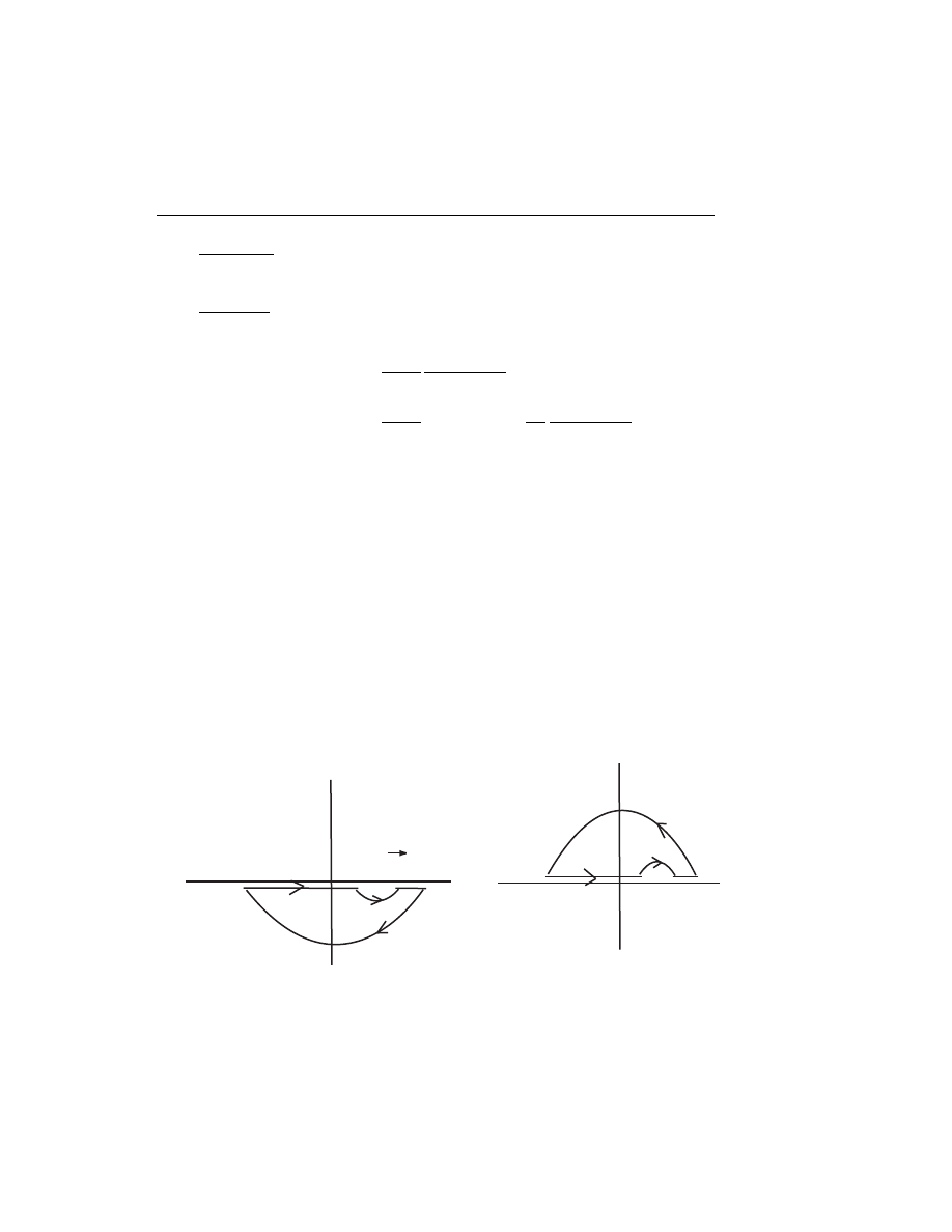
3.6. PROPAGATOR THEORY
53
Example Derive the position space Green function leaving the
pole on the Real axis.
Solution Substituting for G
0
(p) into G
0
(x
−x
0
) we need to eval-
uate (¯
h = 1)
G
0
(x
− x
0
)
=
Z
d
4
p
(2π)
4
1
ω
− ~p
2
/2m
e
−ip·(x−x
0
)
=
Z
d
3
p
(2π)
3
e
i~
p
·(~x−~x
0
)
Z
∞
−∞
dω
2π
e
−iω(t−t
0
)
ω
− ~p
2
/2m
and we see that the integrand is singular at ω = ~
p
2
/2m. This
simple pole is shown in the figure. We need to decide whether to
integrate in the upper half plane (UHP) or the lower half plane
(LHP). This is dictated by the boundary conditions as follows.
Write ω
≡ Re ω + i Im ω, so that
e
−iω(t−t
0
)
= e
i Re ω(t
−t
0
)
e
+ Im ω(t
−t
0
)
For t
− t
0
> 0, the term e
Im ω(t
−t
0
)
will blow up for Im ω > 0
but will go to zero for Im ω < 0. Thus the boundary condition
t
−t
0
> 0 dictates we integrate in the LHP. Similarly for t
−t
0
< 0
we use the UHP. This is shown in the figure. [See also Halzen
and Martin 148]
X
Re
ω
Im
ω
t < t'
X
Re
ω
Im
ω
t > t'
ω
=
ω
0
=p
2
/2m
C
1
C
Now apply the Cauchy Residue Theorem, and remember coun-
terclockwise integration is a positive sign. In the left figure the
54
CHAPTER 3. FREE KLEIN-GORDON FIELD
coutour does not enclose any poles so that
0 =
Z
ω
0
−δ
−∞
+
Z
C
1
+
Z
∞
ω
0
+δ
+
Z
C
and with
R
C
= 0 (Jordan’s lemma) and lim
δ
→0
we have
Z
∞
−∞
=
−
Z
C
1
Thus for t > t
0
G
0
(x
− x
0
)
t>t
0
=
− + πi
Z
d
3
p
(2π)
3
e
i~
p
·(~x−~x
0
)
1
2π
e
−iω
0
(t
−t
0
)
=
−
i
2
Z
d
3
p
(2π)
3
e
i~
p
·(~x−~x
0
)
e
−iω
0
(t
−t
0
)
with ω
0
≡ ~p
2
/2m. Similarly for t < t
0
we obtain
G
0
(x
− x
0
)
t<t
0
=
− − πi
Z
d
3
p
(2π)
3
e
i~
p
·(~x−~x
0
)
1
2π
e
−iω
0
(t
−t
0
)
=
+
i
2
Z
d
3
p
(2π)
3
e
i~
p
·(~x−~x
0
)
e
−iω
0
(t
−t
0
)
But this violates causality ! If the wave pulse is sent out at t
0
we
do expect a signal at a later time t > t
0
but certainly not at an
earlier time t < t
0
.
Because of the singularity, the integral is not well defined until we specify
the limiting process. Let’s now try a different method for evaluating the
integral that is consistent with the boundary condition, i.e. we want
G
0
(x
− x
0
)
t<t
0
= 0.
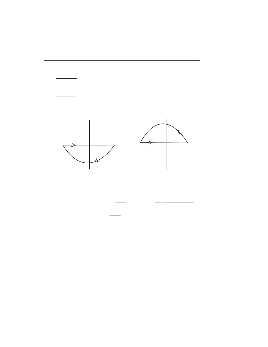
3.6. PROPAGATOR THEORY
55
Example Evaluate the position space Green function by shifting
the pole off the real axis by a small amount ², and take lim
²
→0
.
Solution We can shift the pole either above or below the real
axis. We choose to shift it below because then the upper contour
will enclose no poles and will give a zero integral consistent with
our boundary conditions. This is shown in the figure.
C
t>t’
t<t’
X
ω
0
- i
ε
X
X
ω
0
- i
ε
For t > t
0
we have
∞
R
−∞
+
R
C
= 2πiΣ Residues and with
R
C
= 0 we
get
G
0
(x
− x
0
)
t>t
0
=
−2πi
Z
d
3
p
(2π)
3
e
i~
p
·(~x−~x
0
)
Z
∞
−∞
dω
2π
e
−iω(t−t
0
)
ω
− ~p
2
/2m + i²
=
−i
Z
d
3
p
(2π)
3
e
i~
p
·(~x−~x
0
)
e
−iω
0
(t
−t
0
)
with lim
²
→0
e
²(t
−t
0
)
= 0, which is exactly double our previous answer.
For t < t
0
we get
G
0
(x
− x
0
)
t<t
0
= 0
because no poles are enclosed and this now obeys the boundary
condition.

56
CHAPTER 3. FREE KLEIN-GORDON FIELD
An excellent discussion of all of these issues can be found in [Arfken 4th
ed. 417, 427; Landau 84-88; Bj RQM 85; Cushing 315; Greiner QED 27;
Halzen and Martin 145-150]
The key integral that we have been considering is of the form
I =
Z
∞
−∞
dω
e
−iωt
ω
− ω
0
and with the pole shifted below the real axis this is
I(²) =
Z
∞
−∞
dω
e
−iωt
ω
− ω
0
+ i²
and let’s summarize our results as
I
t>0
=
−πi e
−iω
0
t
I
t<0
= +πi e
−iω
0
t
and
I(²)
t>0
=
−2π i e
−iω
0
t
I(²)
t<0
= 0
When we leave the pole on the real axis the integral
∞
R
−∞
is actually the
Cauchy Principal Value defined as [Arfken 4th ed., p. 417; Landau 88]
P
Z
∞
−∞
f (x)dx
≡ lim
δ
→0
"Z
x
0
−δ
−∞
f (x)dx +
Z
∞
x
0
+δ
f (x)dx
#
with the pole at x = x
0
. As discussed by [Arfken 417, 418] the Cauchy
Principal value is actually a cancelling process. See also [Landau 85-88].
This is because in the vicinity of the simple pole we have
f (x)
≈
a
x
− x
0
which is odd relative to x
0
and so the large singular regions cancel out
[Arfken 4th ed., 417, 418].
The Principal Value Prescription (i.e. our first method with the pole left
on the axis) and the i² Prescription are related. Consider [Merzbacher, old
edition]
1
ω
± i²
=
ω
∓ i²
ω
2
+ ²
2
=
ω
ω
2
+ ²
2
∓
i²
ω
2
+ ²
2
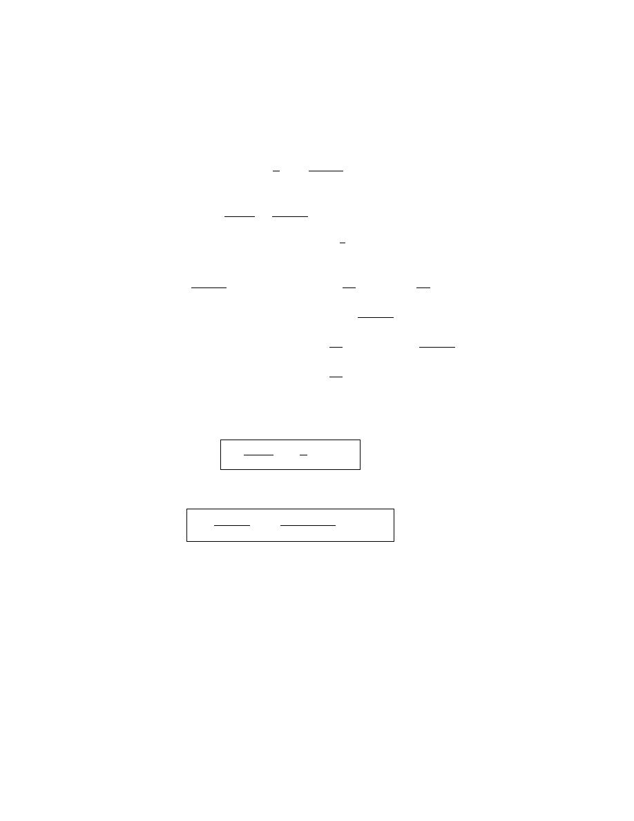
3.6. PROPAGATOR THEORY
57
and using [Merzbacher 3rd ed., p. 631]
δ(x) =
1
π
lim
²
→0
+
²
x
2
+ ²
2
we have
1
ω
± i²
=
ω
ω
2
+ ²
2
∓ iπ δ(ω)
The first term on the right hand side becomes
1
ω
as ²
→ 0 except if ω = 0.
If f (ω) is a well behaved function we have [Merzbacher, old ed., p. 85]
lim
²
→0
Z
∞
−∞
f (ω)
ω
ω
2
+ ²
2
dω
=
lim
²
→0
·Z
−²
−∞
f (ω)
dω
ω
+
Z
∞
²
f (ω)
dω
ω
+
Z
²
−²
f (ω)
ωdω
ω
2
+ ²
2
¸
=
P
Z
∞
−∞
f (ω)
dω
ω
+ f (0) lim
²
→0
Z
²
−²
ωdω
ω
2
+ ²
2
=
P
Z
∞
−∞
f (ω)
dω
ω
+ 0
where the last integral vanishes because the integrand is an odd function of
ω. Thus we can write [Merzbacher, old ed., p. 85]
lim
²
→0
1
ω
± i²
= P
1
ω
∓ iπ δ(ω)
and we can also write [Cushing 315] (with the pole at ω = ω
0
instead of
ω = 0)
P
Z
f (ω)dω
ω
− ω
0
=
Z
f (ω)dω
ω
− ω
0
± i²
± iπ f(ω
0
)

58
CHAPTER 3. FREE KLEIN-GORDON FIELD
Example Verify the above formula for our previous integral
I =
R
dω
e
−iωt
ω
−ω
0
.
Solution For t > 0 we had
P
Z
e
−iωt
dω
ω
− ω
0
=
−πi e
−iω
0
t
and
Z
e
−iωt
dω
ω
− ω
0
+ i²
=
−2πi e
−iω
0
t
Now f (ω
0
) = e
−iω
0
t
, so that
Z
e
−iωt
dω
ω
− ω
0
+ i²
+ iπ f (ω
0
)
=
−2πi e
−iω
0
t
+ πi e
−iω
0
t
=
−πi e
−iω
0
t
=
P
Z
e
−iωt
dω
ω
− ω
0
in agreement with the formula. For t < 0 we had
P
Z
e
−iωt
dω
ω
− ω
0
= +πi e
−iω
0
t
and
Z
e
−iωt
dω
ω
− ω
0
+ i²
= 0
so that
Z
e
−iωt
dω
ω
− ω
0
+ i²
+ iπ f (ω
0
)
=
0 + iπ e
−iω
0
t
=
P
Z
e
−iωt
dω
ω
− ω
0
also in agreement with the formula.

3.6. PROPAGATOR THEORY
59
Example Show that the θ function defined as
θ(t
− t
0
) =
(
1
if
t > t
0
0
if
t < t
0
can be written as
θ(t
− t
0
) = lim
²
→0
−1
2πi
Z
∞
−∞
dω
e
−iω(t−t
0
)
ω + i²
Solution We showed previously that with I(²)
≡
∞
R
−∞
dω
e
−iωt
ω
−ω
0
+i²
we get
I(²)
t>0
=
−2πi e
−iω
0
t
I(²)
t<0
= 0
Replacing t with t
− t
0
and ω
0
= 0 gives I =
R
dω
e
−iω(t−t0)
ω+i²
and
I
t>t
0
=
−2πi
I
t<t
0
= 0
which verifies the above integral representation of θ.
Now let’s finish the job of evaluating the position space Green function
[Bj RQM 84, Greiner QED 27, Kaku 73-74]

60
CHAPTER 3. FREE KLEIN-GORDON FIELD
Example Evaluate the position space Green function, consistent
with the causality boundary condition, in terms of θ(t
−t
0
). Also
write the answer in terms of the plane wave states
φ
p
(x)
≡
e
−ip·x
(2π)
3/2
Solution To satisfy causality we use the i² prescription to eval-
uate the integral which gave
G
0
(x
− x
0
)
t>t
0
=
−i
Z
d
3
p
(2π)
3
e
i~
p
·(~x−~x
0
)
e
−iω
0
(t
−t
0
)
and
G
0
(x
− x
0
)
t<t
0
= 0
with ω
0
≡ ~p
2
/2m. This can be written
G
0
(x
− x
0
) =
−i
Z
d
3
p
(2π)
3
e
i~
p
·(~x−~x
0
)
−iω
0
(t
−t
0
)
θ(t
− t
0
)
Using the plane wave states we have
φ
p
(x)φ
∗
p
(x
0
)
=
1
(2π)
3
e
−ip·x
e
ip
·x
0
=
1
(2π)
3
e
−ip·(x−x
0
)
=
1
(2π)
3
e
−i[ω(t−t
0
)
−~p·(~x−~x
0
)]
giving
G
0
(x
− x
0
) =
−iθ(t − t
0
)
Z
d
3
p φ
p
(x)φ
∗
p
(x
0
)
[Bj RQM 86, Kaku 74]
Finally the d
3
p integrating gives (see Problems) [Bj RQM 86]
G
0
(x
− x
0
) =
−i
µ
m
2πi(t
− t
0
)
¶
3/2
e
im
|~x−~x0|2
2(t
−t0)
θ(t
− t
0
)
See footnote in [Bj RQM 86] discussing the Schrodinger equation
and the Diffusion equation.

3.6. PROPAGATOR THEORY
61
Klein-Gordon Propagator
We originally wrote the Klein-Gordon propagator ∆
F
(k) =
1
k
2
−m
2
but
then digressed on a lengthy discussion of the Schrodinger propagator in order
to illustrate the integration techniques. We now return to the Klein-Gordon
propagator. Consider the following i² prescription
∆
F
(k) =
1
k
2
− m
2
+ i²
Write this as
1
k
2
− m
2
+ i²
=
1
k
2
0
− ~k
2
− m
2
+ i²
=
1
k
2
0
− E
2
+ i²
with E
≡ +
q
~
k
2
+ m
2
We can show (see Problems)
1
k
2
− m
2
+ i²
=
1
k
2
0
− E
2
+ i²
=
1
2k
0
·
1
k
0
− E + i²
+
1
k
0
+ E
− i²
¸
Recall that the momentum space propagator ∆
F
(k) was defined in terms of
the Fourier transform
∆
F
(x
− y) =
Z
d
4
k
(2π)
4
e
−ik.(x−y)
∆
F
(k)
Performing the integration as before we get, with d
˜
˜
k
≡
d
3
k
(2π)
3
2ω
k
(see Prob-
lems)
∆
F
(x
− x
0
) =
−iθ(t − t
0
)
Z
d
˜
˜
k e
−ik·(x−x
0
)
− iθ(t
0
− t)
Z
d
˜
˜
k e
ik
·(x−x
0
)
=
−iθ(t − t
0
)
Z
d
˜
˜
k φ
k
(x)φ
∗
k
(x
0
)
− iθ(t
0
− t)
Z
d
˜
˜
k φ
∗
k
(x)φ
k
(x
0
)

62
CHAPTER 3. FREE KLEIN-GORDON FIELD
Example Show that i∆
F
(x
− x
0
) =
h0|T φ(x)φ(x
0
)
|0i
(Note this is also equal to
=
h0|T φ(x)φ
†
(x
0
)
|0i
for Hermitian fields [BjRQF42].)
Solution The time ordered product is
T A(t
1
)B(t
2
)
≡
(
A(t
1
)B(t
2
)
if
t
1
> t
2
B(t
2
)A(t
1
)
if
t
2
> t
1
≡ θ(t
1
− t
2
)A(t
1
)B(t
2
) + θ(t
2
− t
1
)B(t
2
)A(t
1
)
Thus for the fields
T φ(x)φ(x
0
) = θ(t
− t
0
)φ(x)φ(x
0
) + θ(t
0
− t)φ(x
0
)φ(x)
or
h0|T φ(x)φ(x
0
)
|0i = θ(t − t
0
)
h0|φ(x)φ(x
0
)
|0i + θ(t
0
− t)h0|φ(x
0
)φ(x)
|0i
Thus we want to evaluate
h0|φ(x)φ(x
0
)
|0i and h0|φ(x
0
)φ(x)
|0i. Now
φ(x) =
Z
d˜
k (a
~
k
e
−ik·x
+ a
†
~
k
e
ik
·x
)
with d˜
k
≡
d
3
k
√
(2π)
3
2ω
and ω
≡
q
~
k
2
+ m
2
and ω
0
≡
q
~
k
02
+ m
2
. Evaluate
h0|φ(x)φ(x
0
)
|0i
=
h0|
(2π)
3
Z
d
3
k
√
2ω
d
3
k
0
√
2ω
0
(a
~
k
e
−ik·x
+ a
†
~
k
e
ik
·x
)(a
~
k
0
e
−ik
0
·x
0
+ a
†
~
k
0
e
ik
0
·x
0
)
|0i
=
Z
d˜
k d˜
k
0
h0|a
~
k
a
~
k
0
e
−i(k·x+k
0
·x
0
)
+ a
~
k
a
†
~
k
0
e
−i(k·x−k
0
·x
0
)
+a
†
~
k
a
~
k
0
e
i(k
·x−k
0
·x
0
)
+ a
†
~
k
a
†
~
k
0
e
i(k
·x+k
0
·x
0
)
|0i
However a
~
k
|0i = 0 and h0|a
†
k
= 0. Thus the 1st, 3rd and 4th terms are zero.
We are only left with
h0|a
~
k
a
†
~
k
0
|0i = δ(~k − ~k
0
)
3.6. PROPAGATOR THEORY
63
Continuing
h0|φ(x)φ(x
0
)
|0i =
1
(2π)
3
Z
d
3
k
√
2ω
d
3
k
0
√
2ω
0
δ(~
k
− ~k
0
)e
−i(ωt−~k·~x−ω
0
t
0
+~
k
0
·~x
0
)
=
1
(2π)
3
Z
d
3
k
2ω
e
i~
k.(~
x
−~x
0
)
−iω(t−t
0
)
=
1
(2π)
3
Z
d
3
k
2ω
e
−ik·(x−x
0
)
Obviously we also have
h0|φ(x
0
)φ(x)
|0i =
1
(2π)
3
Z
d
3
k
2ω
e
−ik·(x
0
−x)
=
1
(2π)
3
Z
d
3
k
2ω
e
ik
·(x−x
0
)
Thus
h0|T φ(x)φ(x
0
)
|0i = θ(t − t
0
)
h0|φ(x)φ(x
0
)
|0i + θ(t
0
− t)h0|φ(x
0
)φ(x)
|0i
= θ(t
− t
0
)
Z
d
3
k
(2π)
3
2ω
e
−ik·(x−x
0
)
+ θ(t
0
− t)
Z
d
3
k
(2π)
3
2ω
e
ik
·(x−x
0
)
= i∆
F
(x
− x
0
)

64
CHAPTER 3. FREE KLEIN-GORDON FIELD
Other Propagators
Recall that
φ(x)
=
Z
d˜
k[a
~
k
e
−ik·x
+ a
†
~
k
e
ik
·x
]
≡ φ
+
(x) + φ
−
(x)
[Kaku 152; Mandl & Shaw 44]
From this we can define other propagators (see Problems)
i∆
±
(x
− y) ≡ [φ
±
(x), φ
∓
(y)] =
±
Z
d
3
k
(2π)
3
2ω
~
k
e
∓ik·(x−y)
where ω
~
k
≡ +
q
~
k
2
+ m
2
giving (see Problems)
i∆(x
− y) ≡ [φ(x), φ(y)] = i∆
+
(x
− y) + i∆
−
(x
− y)
or just ∆(x) = ∆
+
(x) + ∆
−
(x). Thus one has [Mandl & Shaw 51]
∆(x)
=
∆
+
(x) + ∆
−
(x) =
−1
(2π)
3
Z
d
3
k
ω
~
k
sin k
· x
=
−i
(2π)
3
Z
d
4
k δ(k
2
− m
2
)²(k
0
)e
−ik·x
with ²(k
0
) =
k
0
|k
0
|
=
(
+1
for
k
0
> 0
−1 for k
0
< 0
Note also that ∆
−
(x) =
−∆
+
(
−x)
These propagators are related to the Feynman propagator by [Mandl
and Shaw 54]
∆
F
(x) = θ(t)∆
+
(x)
− θ(−t)∆
−
(x)
or [Schwabl 283]
∆
F
(x
− x
0
) = θ(t
− t
0
)∆
+
(x
− x
0
)
− θ(t
0
− t)∆
−
(x
− x
0
)
which can be written [Schwabl 283, Mandl and Shaw 54]
∆
F
(x) =
±∆
±
(x) for t
>
<
0

3.6. PROPAGATOR THEORY
65
Example Show that
∆
F
(x
− x
0
) = θ(t
− t
0
)∆
+
(x
− x
0
)
− θ(t
0
− t)∆
−
(x
− x
0
)
where
i∆
F
(x
− x
0
) =
h0|T φ(x)φ(x
0
)
|0i
and
i∆
±
(x
− y) ≡ [φ
±
(x), φ
∓
(y)].
Solution
i∆
F
(x
− x
0
)
=
h0|T φ(x)φ(x
0
)
|0i
=
θ(t
− t
0
)
h0|φ(x)φ(x
0
)
|0i + θ(t
0
− t)h0|φ(x
0
)φ(x)
|0i
Thus to do this problem we really need to show that
h0|φ(x)φ(x
0
)
|0i = [φ
+
(x), φ
−
(x
0
)]
and
h0|φ(x
0
)φ(x)
|0i = −[φ
−
(x), φ
+
(x
0
)]
Let’s only do the first of these. The question is, how do these relations
come about ? The answer is easy. Commutators are just c-numbers, i.e.
classical functions or numbers. Thus
h0|c|0i = ch0|0i = c for any c-number.
Therefore
[φ
+
(x), φ
−
(x
0
)]
=
h0|[φ
+
(x), φ
−
(x
0
)]
|0i
=
h0|φ
+
(x)φ
−
(x
0
)
|0i − h0|φ
−
(x
0
)φ
+
(x)
|0i
=
h0|φ
+
(x)φ
−
(x
0
)
|0i
because φ
+
|0i = 0.
Now φ = φ
+
+ φ
−
. Thus
φ
|0i = φ
+
|0i + φ
−
|0i = 0 + φ
−
|0i = φ
−
|0i
and similarly
h0|φ = h0|φ
+
giving
[φ
+
(x), φ
−
(x
0
)] =
h0|φ(x)φ(x
0
)
|0i
as required. (Proof of the other relation follows similarly).

66
CHAPTER 3. FREE KLEIN-GORDON FIELD
3.7
Complex Klein-Gordon Field
[Schwabl 285; Kaku 69; Huang 24-25]
[W. Pauli and V. F. Weisskopf, Helv. Phys. Acta, 7, 709 (1934)]
Charged particles cannot be described with a real scalar field because it
only has one component, whereas a minimum of two components is needed
to describe charge. Define
φ
≡
1
√
2
(φ
1
+ iφ
2
) and φ
†
≡
1
√
2
(φ
1
− iφ
2
)
where φ
1
and φ
2
are real fields. The normalization factor
1
√
2
is chosen so
that φ
i
has the same renormalization as the real scalar field discussed before.
A suitable classical Lagrangian is (with
|φ|
2
= φφ
†
) [Huang 24]
L = ∂
µ
φ
†
∂
µ
φ
− m
2
|φ|
2
=
1
2
2
X
i=1
(∂
µ
φ
i
∂
µ
φ
i
− m
2
φ
2
i
)
which is just the sum of the Lagrangian for the real fields.
The Euler-Lagrange equations give the equations of motion [Schwabl
285]
(
2
2
+ m
2
)φ = 0 and (
2
2
+ m
2
)φ
†
= 0
with the conjugate momenta being [Kaku 70; Schwabl 285]
Π = ˙
φ
†
and Π
†
= ˙
φ
with the equal time commutation relations [Kaku 70; Schwabl 285]
[φ(~
x, t), Π(~
x
0
, t)] = [φ(~
x, t), ˙
φ
†
(~
x
0
, t)] = iδ(~
x
− ~x
0
)
[φ
†
(~
x, t), Π
†
(~
x
0
, t)] = [φ
†
(~
x, t), ˙
φ(~
x
0
, t)] = iδ(~
x
− ~x
0
)
and [Schwabl 285]
[φ(~
x, t), φ(~
x
0
, t)] = [Π(~
x, t), Π(~
x
0
, t)] = 0
[φ
†
(~
x, t), φ
†
(~
x
0
, t)] = [Π
†
(~
x, t), Π
†
(~
x
0
, t)] = 0
We Fourier expand each component φ
i
(x) exactly as before [Kaku 70; Huang
24]
φ
i
(x) =
Z
d˜
k (a
i~
k
e
−ik·x
+ a
†
i~
k
e
ik
·x
)

3.7. COMPLEX KLEIN-GORDON FIELD
67
where the commutation relations are [Kaku 70; Huang 25]
[a
i~
k
, a
†
j~
k
0
] = δ(~
k
− ~k
0
)δ
ij
However rather than treating the i fields separately, we can combine them
as we did with the wave functions φ(x). Define [Kaku 70; Huang 25]
a
~
k
≡
1
√
2
(a
1~
k
+ ia
2~
k
) and b
~
k
≡
1
√
2
(a
1~
k
− ia
2~
k
)
so that the Fourier expansion now becomes [Huang 25; Schwabl 285]
φ(x) =
Z
d˜
k (a
~
k
e
−ik·x
+ b
†
~
k
e
ik
·x
)
(Exercise: Prove this result) and for the other field, obviously it is
φ
†
(x) =
Z
d˜
k(a
†
~
k
e
ik
·x
+ b
~
k
e
−ik·x
)
The new commutation relations are [Kaku 70; Schwabl 286; Huang 25]
[a
~
k
, a
†
~
k
0
] = [b
~
k
, b
†
~
k
0
] = δ
~
k~
k
0
and
[a
~
k
, a
~
k
0
] = [b
~
k
, b
~
k
0
] = [a
~
k
, b
~
k
0
] = [a
~
k
, b
†
~
k
0
] = 0
There are now two occupation-number operators, for particles a and for
particles b [Schwabl 286]
N
a~
k
≡ a
†
~
k
a
~
k
and N
b~
k
≡ b
†
~
k
b
~
k
where a
†
~
k
and a
~
k
create and annihilate a particles and b
†
~
k
and b
~
k
create and
annihilate b particles. The vacuum state is defined by [Schwabl 286]
a
~
k
|0i = b
~
k
|0i = 0
The four momentum is [Schwabl 286; Mandl and Shaw 49; Greiner FQ 93]
P
µ
= (H, ~
P ) =
X
~
k
k
µ
(N
a~
k
+ N
b~
k
)
giving
H =
X
~
k
ω
~
k
(N
a~
k
+ N
b~
k
)
and
~
P =
X
~
k
~
k(N
a~
k
+ N
b~
k
)

68
CHAPTER 3. FREE KLEIN-GORDON FIELD
3.7.1
Charge and Complex Scalar Field
Recall the real scalar field Lagrangian
L =
1
2
(∂
µ
φ∂
µ
φ
− m
2
φ
2
) and the
complex scalar field Lagrangian
L = ∂
µ
φ
†
∂
µ
φ
− m
2
|φ|
2
=
1
2
2
X
i=1
(∂
µ
φ
i
∂
µ
φ
i
− m
2
φ
2
i
)
with
|φ|
2
≡ φφ
†
. The complex scalar field Lagrangian (and action) is invari-
ant under the transformation
φ(x)
→ e
iqθ
φ(x)
φ
†
(x)
→ e
−iqθ
φ
†
(x)
which generates a U (1) symmetry [Kaku 70]. Recall that before we had (for
small α
i
= ²
i
)
η
r
(x)
→ η
0
r
(x) = e
iα
i
X
i
η
r
(x)
≈ (1 + i²
i
X
i
)η
r
(x)
giving
δη
r
(x) = η
0
r
(x)
− η
r
(x) = i²
i
X
i
η
r
(x)
Our two fields are η
1
≡ φ and η
2
≡ φ
†
giving (with small θ = ²)
δφ(x) = iq²φ(x)
and
δφ
†
(x) =
−iq²φ
†
(x)
Recall the Noether current
j
µ
≡
∂
L
∂(∂
µ
η
r
)
∆η
r
− T
µν
δx
ν
with
T
µν
≡
∂
L
∂(∂
µ
η
r
)
∂
ν
η
r
− g
µν
L
Also recall the relation between local and total variations
δη
r
(x) = ∆η
r
(x)
−
∂η
r
∂x
µ
δx
µ
For δx
ν
= 0, we have δη(x) = ∆η(x) [Schwabl 272] and therefore
j
µ
=
∂
L
∂(∂
µ
η
r
)
δη
r
=
∂
L
∂(∂
µ
φ)
δφ +
∂
L
∂(∂
µ
φ
†
)
δφ
†
=
∂
L
∂(∂
µ
φ)
iq²φ +
∂
L
∂(∂
µ
φ
†
)
(
−i)q²φ
†

3.7. COMPLEX KLEIN-GORDON FIELD
69
and with
L = ∂
µ
φ
†
∂
µ
φ
− m
2
φφ
†
= g
µν
∂
ν
φ
†
∂
µ
φ
− m
2
φφ
†
gives
∂
L
∂(∂
µ
φ)
= g
µν
∂
ν
φ
†
= ∂
µ
φ
†
and
∂
L
∂(∂
µ
φ
†
)
= ∂
µ
φ
Thus the Noether current is
j
µ
= (∂
µ
φ
†
)iq²φ
− (∂
µ
φ)iq²φ
†
Once again we drop the constant factor ² and insert a minus sign to
define a new current [Kaku 71, Mosel 19, Schwabl 286, Huang 25]
j
µ
= iq[(∂
µ
φ)φ
†
− (∂
µ
φ
†
)φ]
which agrees exactly with the 4-current derived previously!
The conserved charge (
dQ
dt
= 0) is therefore [Kaku 71, Mosel 19]
Q
=
Z
d
3
x j
o
= iq
Z
d
3
x( ˙
φφ
†
− ˙φ
†
φ)
=
q
Z
d
3
k(a
†
~
k
a
~
k
− b
†
~
k
b
~
k
)
=
q
Z
d
3
k(N
a~
k
− N
b~
k
)
(Exercise: Prove this result). Here j
o
matches exactly our expression for ρ
derived previously! [Kaku 71] gives an excellent discussion of the physical
interpretation of this charge. Also note that “charge” is used in a generic
sense [Huang 26] since electromagnetic coupling has not yet been turned on.
Compare this to our result from Chapter 1 which was (with probability
current density j
µ
= (ρ,~j ) = ¯
ψγ
µ
ψ )
Q
=
Z
d
3
x j
0
= q
Z
d
3
x ¯
ψ γ
0
ψ
=
q
Z
d
3
x ρ
where the probability density was ρ = ¯
ψγ
0
ψ = ψ
†
γ
0
γ
0
ψ = ψ
†
ψ. This was an
expression in terms of the classical Dirac field ψ. Above we now have Q in
terms of the quantized field operators a, a
†
, b, b
†
for the complex scalar field.

70
CHAPTER 3. FREE KLEIN-GORDON FIELD
3.8
Summary
Two useful integrals are:
1
(2π)
3
Z
d
3
xe
±i(~k−~k
0
).~
x
= δ(~
k
− ~k
0
)
δ
4
(x
− y) =
Z
d
4
k
(2π)
4
e
−ik·(x−y)
3.8.1
KG classical field
The massive Klein-Gordon Lagrangian is
L
KG
=
1
2
(∂
µ
φ∂
µ
φ
− m
2
φ
2
)
giving the KGE (using p
2
→ −2
2
)
(
2
2
+ m
2
)φ = 0
(p
2
− m
2
)φ = 0
The covariant momentum density is
Π
µ
= ∂
µ
φ
giving the canonical momentum
Π
≡ Π
o
= ˙
φ(x)
and Hamiltonian density
H =
1
2
[Π
2
+ ( ~
∇φ)
2
+ m
2
φ
2
]
and momentum
~
P =
−
Z
d
3
x ˙
φ(x) ~
∇φ(x)
The Fourier expansion of the KG field is
φ(~
x, t)
≡ φ
+
(x) + φ
−
(x) =
Z
d˜
k
h
a
~
k
e
−ik·x
+ a
†
~
k
e
ik
·x
i
The conjugate momentum is
Π(~
x, t) = ˙
φ(~
x, t)
≡ Π
+
(x) + Π
−
(x)
=
−i
Z
d˜
k ω
h
a
~
k
e
−ik·x
− a
†
~
k
e
ik
·x
i

3.8. SUMMARY
71
In the above equations (with k
0
≡ ω = +
q
~
k
2
+ m
2
)
d˜
k
≡
d
3
k
p
2ω(2π)
3
=
s
2ω
(2π)
3
d
4
kδ(k
2
− m
2
) θ(k
o
)
The integrals are cast into discrete form with the replacement
Z
d
3
k
→ Σ
~
k
.
3.8.2
Klein-Gordon Quantum field
To develop the QFT we impose the equal time commutation relations
[φ(~
x, t), Π(~
x
0
, t)] = iδ(~
x
− ~x
0
)
and
[φ(~
x, t), φ(~
x
0
, t)] = [Π(~
x, t), Π(~
x
0
, t)] = 0
which imply
[a(~
k), a
†
(~
k
0
)] = δ(~
k
− ~k
0
)
and
[a(~
k), a(~
k
0
)] = [a
†
(~
k), a
†
(~
k
0
)] = 0
Defining
N
~
k
≡ a
†
~
k
a
~
k
the Hamiltonian and momentum can be re-written as
H =
Z
d
3
k
µ
N
~
k
+
1
2
¶
ω
~
P =
Z
d
3
k
µ
N
~
k
+
1
2
¶
~
k
The vacuum state is defined via
a
~
k
|0i = 0
and the many body states are
| · · · n
~
k
i
· · · n
~
k
j
· · ·i =
Y
i
|n
~
k
i
i
with
|n
~
k
i
i =
1
q
n
~
k
!
³
a
†
~
k
´
n
~
k
|0i
H
| · · · n
~
k
i
· · · n
~
k
j
· · ·i =
X
~
k
n
k
²(~
k)
| · · · n
~
k
i
· · · n
~
k
j
· · ·i
where ²(~
k) = ¯
hω(~
k).

72
CHAPTER 3. FREE KLEIN-GORDON FIELD
3.8.3
Propagator Theory
The non-free KGE is
(
2
2
+ m
2
)φ = J (x)
The Feynman propagator in position space is defined as
(
2
2
+ m
2
)∆
F
(x
− y) ≡ −δ
4
(x
− y)
so that the solution to the non-free KGE is
φ(x) = φ
0
(x)
−
Z
d
4
y ∆
F
(x
− y)J(y)
where φ
0
(x) is the solution with J = 0. The momentum space Feynman
propagator is defined through the Fourier transform
∆
F
(x
− y) ≡
Z
d
4
k
(2π)
4
e
−ik·(x−y)
∆
F
(k)
The usual method of solution for propagators or Green functions is to solve
for ∆
F
(k) and then do a contour integral to get ∆
F
(x
− y) rather than
solving for ∆
F
(x
− y) directly. We get
∆
F
(k) =
1
k
2
− m
2
which is the inverse of the momentum operator in the free KGE. This finally
leads to
∆
F
(x
− x
0
) =
−iθ(t − t
0
)
Z
d˜
k e
−ik·(x−x
0
)
− iθ(t
0
− t)
Z
d˜
k e
ik
·(x−x
0
)
One can also show that
i∆
F
(x
− x
0
)
=
h0|T φ(x)φ(x
0
)
|0i
=
h0|T φ(x)φ
†
(x
0
)
|0i
where the second line is true for Hermitian fields [BjRQF42].
Other useful propagators are
i∆
±
(x
− y) ≡ [φ
±
(x), φ
∓
(y)] =
±
Z
d
˜
˜
ke
∓ik·(x−y)
giving
i∆(x
− y) ≡ [φ(x), φ(y)] = −i∆
+
(x
− y) + i∆
−
(x
− y)

3.9. REFERENCES AND NOTES
73
with
∆(x)
=
∆
+
(x) + ∆
−
(x) =
−
Z
d
3
k
(2π)
3
ω
~
k
sin k
· x
These other propagators are related to the Feynman propagator by
∆
F
(x) = θ(t)∆
+
(x)
− θ(−t)∆
−
(x)
or
∆
F
(x) =
±∆
±
(x) for
t
>
<
0
3.8.4
Complex KG field
Not summarized; see text.
3.9
References and Notes
Good references for this chapter are [Teller, Bergstrom and Goobar, Roman,
Halzen and Martin, Muirhead, Leon, Goldstein].

74
CHAPTER 3. FREE KLEIN-GORDON FIELD

Chapter 4
Dirac Field
We have seen that the KGE gives rise to negative energies and non-positive
definite probabilities and for these reasons was discarded as a fundamental
quantum equation. These problems arise because the KGE is non-linear in
∂
∂t
, unlike the SE. Dirac thus sought a relativistic quantum equation linear
in
∂
∂t
, like the SE. We shall see that therefore Dirac was forced to invent a
matrix equation.
The ‘derivation’ of the DE presented here follows [Griffiths, pg. 215].
Dirac was searching for an equation linear in E or
∂
∂t
. Instead of starting
from
p
2
− m
2
= 0
his strategy was to factor this relation, which is easy if we only have p
0
(i.e.
~
p = 0), namely (with p
0
= p
0
)
(p
0
− m)(p
0
+ m) = 0
and obtain two first order equations
p
0
− m = 0 or p
0
+ m = 0
However it’s more difficult if ~
p is included. Then we are looking for some-
thing of the form p
2
− m
2
= p
µ
p
µ
− m
2
= (β
µ
p
µ
+ m)(γ
ν
p
ν
− m) where β
µ
and γ
ν
are 8 coefficients to be determined. The RHS is
β
µ
γ
ν
p
µ
p
ν
+ m(γ
ν
− β
ν
)p
ν
− m
2
For equality with LHS we don’t want terms linear in p
ν
, thus γ
ν
= β
ν
,
leaving
p
2
= p
µ
p
µ
= γ
µ
γ
ν
p
µ
p
ν
75

76
CHAPTER 4. DIRAC FIELD
i.e. (with (p
1
)
2
= (p
1
)
2
)
(p
0
)
2
− (p
1
)
2
− (p
2
)
2
− (p
3
)
2
= (γ
0
)
2
(p
0
)
2
+ (γ
1
)
2
(p
1
)
2
+ (γ
2
)
2
(p
2
)
2
+(γ
3
)
2
(p
3
)
2
+ (γ
0
γ
1
+ γ
1
γ
0
)p
0
p
1
+(γ
0
γ
2
+ γ
2
γ
0
)p
0
p
2
+ (γ
0
γ
3
+ γ
3
γ
0
)p
0
p
3
+(γ
1
γ
2
+ γ
2
γ
1
)p
1
p
2
+ (γ
1
γ
3
+ γ
3
γ
1
)p
1
p
3
+(γ
2
γ
3
+ γ
3
γ
2
)p
2
p
3
Here’s the problem; we could pick γ
0
= 1 and γ
1
= γ
2
= γ
3
= i but
we can’t get rid of the ‘cross terms’. At this point Dirac had a brilliant
inspiration; what if the γ’s are matrices instead of numbers? Since matrices
don’t commute we might be able to find a set such that
(γ
0
)
2
= 1 (γ
1
)
2
= (γ
2
)
2
= (γ
3
)
2
=
−1
γ
µ
γ
ν
+ γ
ν
γ
µ
= 0 for µ
6= ν
Or, more succinctly,
{γ
µ
, γ
ν
} = 2g
µν
which is called a Clifford Algebra
where the curly brackets denote the anti-commutator
{A, B} ≡ AB + BA.
It turns out that this can be done, but the smallest set of matrices are 4
× 4.
These are
γ
0
≡ β =
µ
I
0
0
−I
¶
~
γ
≡ β~α ≡
µ
0
~
σ
−~σ 0
¶
γ
µ
≡ (β, β~α)
Let’s introduce everything else for completeness
γ
5
≡ iγ
0
γ
1
γ
2
γ
3
=
µ
0
I
I
0
¶
σ
1
=
µ
0
1
1
0
¶
σ
2
=
µ
0
−i
i
0
¶
σ
3
=
µ
1
0
0
−1
¶
~
α
≡
µ
0
~
σ
~
σ
0
¶
β
≡
µ
1
0
0
−1
¶
γ
µ
†
= γ
0
γ
µ
γ
0
i.e. γ
0
†
= γ
0
, γ
i
†
=
−γ
i
β
−1
= β
and
γ
5
= γ
5
These conventions are used by the following authors: [Griffiths, Kaku,
Halzen & Martin].
Thus the Dirac equation is (p
− m)ψ = 0 with A ≡ γ
µ
A
µ
. In coordi-
nate space (using p
µ
→ i∂
µ
) it is (i∂
− m)ψ = 0 . In non-covariant notation
it is
Hψ = i¯
h
∂ψ
∂t
with
H
≡ ~α · ~p + βm

4.1. PROBABILITY & CURRENT
77
The DE can be written in terms of 4-vectors (/
p
− m)ψ = 0 and is therefore
manifestly covariant.
4.1
Probability & Current
For the SE and KGE we used SE
∗
and KGE
∗
to derive the continuity equa-
tion. For matrices the generalization of complex conjugate (
∗) is Hermitian
conjugate (
†) which is the transpose of the complex conjugate. The DE is
(i/
∂
− m)ψ = 0 = (iγ
µ
∂
µ
− m)ψ
and DE
†
is (using (AB)
†
= B
†
A
†
)
ψ
†
(i/
∂
− m)
†
= 0
= ψ
†
(
−iγ
µ
†
∂
µ
− m) = 0 where ∂
†
µ
= ∂
µ
= ψ
†
(
−iγ
0
γ
µ
γ
0
∂
µ
− m) = 0 using γ
µ
†
= γ
0
γ
µ
γ
0
We want to introduce the Dirac adjoint (ψ is a column matrix)
¯
ψ
≡ ψ
†
γ
0
( ¯
ψ is a row matrix!)
Using γ
0
γ
0
= 1 we get
ψ
†
(
−iγ
0
γ
µ
γ
0
∂
µ
− mγ
0
γ
0
) = 0
⇒ ¯
ψ(iγ
µ
γ
0
∂
µ
+ mγ
0
) = 0
and cancelling out γ
0
gives, the Dirac adjoint equation,
¯
ψ(i/
∂ + m) = 0
⇔ ¯
ψ(i
←
/
∂ + m) = 0
Some sloppy authors write this as (i/
∂ + m) ¯
ψ = 0 but this cannot be because
¯
ψ is a row matrix! The notation
←
/
∂ however means that /
∂ operates on ¯
ψ to
the left, i.e. ¯
ψ
←
/
∂
≡ (∂
µ
¯
ψ)γ
µ
.
It’s very important not to get confused with this. The DE and DE
†
are
explicitly
(i/
∂
− m)ψ = 0 ⇔ iγ
µ
∂
µ
ψ
− mψ = 0
¯
ψ(i/
∂ + m) = 0
⇔ i(∂
µ
¯
ψ)γ
µ
+ m ¯
ψ = 0

78
CHAPTER 4. DIRAC FIELD
Now let’s derive the continuity equation. Multiply DE from the left by ¯
ψ
and DE
†
from the right by ψ. Now one could get very confused writing
¯
ψ(i/
∂
− m)ψ = 0
¯
ψ(i/
∂ + m)ψ = 0
whereas what is really meant is [Halzen & Martin, pg. 103]
¯
ψ(iγ
µ
∂
µ
ψ
− mψ) = 0
(i(∂
µ
¯
ψ)γ
µ
+ m ¯
ψ)ψ = 0
Adding these gives
¯
ψγ
µ
∂
µ
ψ + (∂
µ
¯
ψ)γ
µ
ψ = 0 = ∂
µ
( ¯
ψγ
µ
ψ)
giving
j
µ
= ( ¯
ψγ
µ
ψ)
≡ (ρ,~j)
or
ρ = ¯
ψγ
0
ψ = ψ
†
ψ =
4
X
i=1
|ψ
i
|
2
which is now positive definite! The 3-current is
~j = ¯
ψ~
γψ
[see also Mosel 17, 34]
4.2
Bilinear Covariants
ψ can be written
ψ
1
ψ
2
ψ
3
ψ
4
and one can try to construct a scalar, such as
ψ
†
ψ = (ψ
∗
1
ψ
∗
2
ψ
∗
3
ψ
∗
4
)
ψ
1
ψ
2
ψ
3
ψ
4
=
|ψ
1
|
2
+
|ψ
2
|
2
+
|ψ
3
|
2
+
|ψ
4
|
2
but this is not
a Lorentz scalar (it’s got all + signs).
Rather, define the Dirac adjoint
¯
ψ
≡ ψ
†
γ
0
= (ψ
∗
1
ψ
∗
2
− ψ
∗
3
− ψ
∗
4
)

4.3. NEGATIVE ENERGY AND ANTIPARTICLES
79
and ¯
ψψ =
|ψ
1
|
2
+
|ψ
2
|
2
− |ψ
3
|
2
− |ψ
4
|
2
is a Lorentz scalar (see Bjorken and
Drell]. One can prove that the following quantities transform as indicated:
¯
ψψ
scalar
(1 component)
¯
ψγ
5
ψ
pseudoscalar
(1 component)
¯
ψγ
µ
ψ
vector
(4 component)
¯
ψγ
µ
γ
5
ψ
pseudovector
(4 component)
¯
ψσ
µν
ψ
antisymmetric 2nd rank tensor
(6 component)
where σ
µν
≡
i
2
(γ
µ
γ
ν
− γ
ν
γ
µ
).
4.3
Negative Energy and Antiparticles
4.3.1
Schrodinger Equation
The free particle SE is
−
¯
h
2
2m
∇
2
ψ = i¯
h
∂ψ
∂t
which has solution
ψ(x, t) = (C cos kx + D sin kx) e
i
¯
h
Et
≡ ψ
E
=
³
Ae
ikx
+ Be
−ikx
´
e
i
¯
h
Et
in 1-dimension.
Substituting gives
¯
hk
2
2m
ψ(x, t) =
−Eψ(x, t) or
Ã
E +
¯
h
2
k
2
2m
!
ψ = 0
yielding
E =
−
¯
h
2
k
2
2m
However it also has solution ψ(x, t) = (Ae
ikx
+ Be
−ikx
)e
−
i
¯
h
Et
≡ ψ
−E
Substituting gives
¯
h
2
k
2
2m
ψ(x, t) = +Eψ(x, t) or
Ã
E
−
¯
h
2
k
2
2m
!
ψ = 0
yielding
E = +
¯
h
2
k
2
2m

80
CHAPTER 4. DIRAC FIELD
ψ
E
and ψ
−E
are different solutions. The first one ψ
E
corresponds to positive
energy and the second one ψ
−E
to negative energy. We are free to toss away
one solution as unphysical and only keep ψ
E
.
However for KGE and DE the same solution ψ gives both positive and
negative energy. Of course we are not free to toss away one energy because
it’s in the solution. Whereas in the SE we got two different solutions for
positive and negative energy. If we want to get rid of negative energy in the
SE we toss away one solution. However in KGE and DE we always get both
positive and negative energy for all solutions. The only way to toss away
negative energy is to toss away all solutions; i.e. toss out the whole equation!
?Also reason why Einstein did not reject SR; E =
±
p
~
p
2
+ m
2
were
separate solutions; not part of same solution.
4.3.2
Klein-Gordon Equation
The free particle KGE is
(
2
2
+ m
2
)φ = 0
with
2
2
=
−
∂
2
∂t
2
+
∇
2
A solution is
φ = N e
ip
·x
= N e
i(Et
−~p·~x)
Substituting gives
(E
2
− ~p
2
+ m
2
)φ = 0
which implies
⇒ E
2
= ~
p
2
+ m
2
or
E =
±
q
~
p
2
+ m
2
Thus the single solution φ = N e
ip
·x
has both positive and negative energy
solutions. Another solution is
φ = N e
−ip·x
= N e
−i(Et−~p·~x)
Substituting also gives the same as above, namely (E
2
− ~p
2
+ m
2
)φ = 0 or
E =
±
q
~
p
2
+ m
2
4.3. NEGATIVE ENERGY AND ANTIPARTICLES
81
and again the single solution φ = N e
−ip·x
has both positive and negative
energy solutions.
The interpretation of these states is as follows. For ~
p = 0 (particle at rest)
then E =
±m. For ~p 6= 0, there will be a continuum of states above and
below E =
±m [Landau, pg. 225], with bound states appearing in between.
In QM there would be transitions to the negative energy continuum to infi-
nite negative energy. This also happens with the Dirac equation. However,
the DE describes, automatically, particles with spin. Dirac’s way out of the
negative energy catastrophe was to postulate that the negative energy sea
was filled with fermions and so the ???
E < 0
E > 0
E
- mc
0
p = 0
2
mc
2
p = 0
However for the KGE the negative energies are a catastrophe.
Also we can now clearly see the problem with ρ as calculated with the
KGE. Recall ρ =
i¯
h
2m
³
φ
∗ ∂φ
∂t
− φ
∂φ
∗
∂t
´
. For φ = e
±ip·x
we get ρ =
∓
¯
h
m
φ
∗
φE
which gives negative ρ for positive or negative E. (Halzen & Martin, pg. 74]
82
CHAPTER 4. DIRAC FIELD
4.3.3
Dirac Equation
Let’s look for plane wave solutions of the form ψ(x) = w(~
p)e
−ip·x
. Substi-
tuting into (i/
∂
− m)ψ = 0 gives the momentum space DE (/p− m)w = 0 .
Actually, let’s first look at rest frame (~
p = 0) solutions (RF). Writing the
DE as
Hψ = i¯
h
∂ψ
∂t
with H = ~
α
· ~p + βm
independent DE is Hψ = Eψ, which in the RF is
Hw = βmw =
Ã
mI
0
0
−mI
!
w = Ew,
The eigenvalues are E = m, m,
−m, −m with eigenvectors [Halzen & Martin,
pg. 104]
1
0
0
0
0
1
0
0
0
0
1
0
0
0
0
1
Thus the DE has positive (E = +m) and negative (E =
−m) energy solu-
tions! (We shall look at ~
p
6= 0 solutions in a moment)
Let’s summarize so far (Aitchison & Hey, pg. 71)
Probability (ρ)
Energies for same solution ψ
SE
+
+
KGE
−
+,
−
DE
+
+,
−
Thus both the KGE and DE have negative energies.
The DE describes fermions (see next section). Dirac’s idea was that
the negative energy sea was filled with fermions and via PEP prevented the
negative energy cascade of positive energy particles. Dirac realized if given
particles in sea energy of 2mc
2
create holes. Dirac Sea not taken seriously
until positron discovered!! (1932 Anderson)

4.4. FREE PARTICLE SOLUTIONS OF DIRAC EQUATION
83
4.4
Free Particle Solutions of Dirac Equation
Before proceeding recall the following results:
σ
x
=
µ
0
1
1
0
¶
σ
y
=
µ
0
−i
i
0
¶
σ
z
=
µ
1
0
0
−1
¶
~
σ
· ~p =
µ
P
z
p
−
p
+
−p
z
¶
≡
µ
p
z
p
x
− ip
y
p
x
+ ip
y
−p
z
¶
Let’s now look at ~
p
6= 0 solutions (i.e. not in rest frame). As before, we look
for solutions of the form ψ(x) = w(~
p)e
−ip·x
Substituting into (i/
∂
− m)ψ = 0
gives the momentum space DE (/
p
− m)w = 0. Using /p =
µ
E
−~σ · ~p
~
σ
· ~p
−E
¶
gives, with w
≡
µ
w
A
w
B
¶
(/
p
− m)w =
µ
E
− m
−~σ · ~p
~
σ
· ~p
−E − m
¶ µ
w
A
w
B
¶
= 0 =
"
(E
− m) w
A
− ~o · ~p w
B
~
σ
· ~p w
A
− (E + m) w
B
#
giving
w
A
=
~
σ
· ~p
E
− m
w
B
and w
B
=
~
σ
· ~p
E + m
w
A
Combining yields
w
A
=
(~
σ
· ~p )
2
E
2
− m
2
w
A
=
~
p
2
E
2
− m
2
w
A
because (~
σ
· ~p)
2
= ~
p
2
. Thus
E
2
= ~
p
2
+ m
2
or E =
±
q
~
p
2
+ m
2
Thus again we see the negative energy solutions ! (this time for the ~
p
6= 0
DE)
Our final solutions are
w =
µ
w
A
w
B
¶
=
µ
w
A
~
σ
·~p
E+m
w
A
¶
or
µ
~
σ
·~p
E
−m
w
B
w
B
¶
with w
A
and w
B
left unspecified, which means we are free to choose them
[Aitchison & Hey 69] as
w
A
, w
B
=
µ
1
0
¶
or
µ
0
1
¶

84
CHAPTER 4. DIRAC FIELD
We have the following possibilities
Pick w
A
=
µ
1
0
¶
⇒ w
B
=
~
o
· ~p
E + m
µ
1
0
¶
=
1
E + m
µ
p
z
p
+
¶
(1) p
±
≡ p
x
± ip
y
Pick w
A
=
µ
0
1
¶
⇒ w
B
=
~
o
· ~p
E + m
µ
0
1
¶
=
1
E + m
µ
p
−
−p
z
¶
(2)
Pick w
B
=
µ
1
0
¶
⇒ w
A
=
~
o
· ~p
E
− m
µ
1
0
¶
=
1
E
− m
µ
p
z
p
+
¶
(3)
Pick w
B
=
µ
0
1
¶
⇒ w
A
=
~
o
· ~p
E
− m
µ
0
1
¶
=
1
E
− m
µ
p
−
−p
z
¶
(4)
But the question is, do we use E = +
p
~
p
2
+ m
2
or E =
−
p
~
p
2
+ m
2
? Well,
for (1) and (2) we must use E = +√ otherwise
1
E+m
blows up for ~
p = 0.
For (3) and (4) we must use E =
−√ otherwise
1
E
−m
blows up for ~
p = 0.
The term E = +√
is called the particle solution. The term E =
−√ is
called the antiparticle solution.
Rewrite as, with χ
(1)
≡
µ
1
0
¶
and χ
(2)
≡
µ
0
1
¶
w
(1)
(~
p) = N
1
0
p
z
E+m
p
+
E+m
= N
µ
1
~
σ
·~p
E+m
¶
χ
(1)
w
(2)
(~
p) = N
0
1
p
−
E+m
−p
z
E+m
= N
µ
1
~
o
·~p
E+m
¶
χ
(2)
with
E
≡ +
q
~
p
2
+ m
2
and also
w
(3)
(~
p) = N
p
z
E
−m
p
+
E
−m
1
0
= N
µ
~
σ
·~p
E
−m
1
¶
χ
(1)
w
(4)
(~
p) = N
p
−
E
−m
−p
z
E
−m
0
1
= N
µ
~
σ
·~p
E
−m
1
¶
χ
(2)
with
E
≡ −
q
~
p
2
+ m
2

4.4. FREE PARTICLE SOLUTIONS OF DIRAC EQUATION
85
or
w
(s)
(~
p) = N
µ
1
~
o
·~p
E+m
¶
χ
(s)
with E
≡ +
p
~
p
2
+ m
2
w
(s+2)
(~
p) = N
µ
~
σ
·~p
E
−m
1
¶
χ
(s)
with E
≡ −
p
~
p
2
+ m
2
s = 1, 2
[Halzen & Martin, pg. 105]
But all free particles carry positive energy! Thus re-interpret w
(3)
and w
(4)
as positive energy antiparticle states
w
(s+2)
(~
p) = N
Ã
~
σ
·~p
−
√
~
p
2
+m
2
−m
1
!
χ
(s)
w
(s+2)
(
−~p) = N
Ã
−~σ·~p
−
√
~
p
2
+m
2
−m
1
!
χ
(s)
= N
Ã
~
σ
·~p
√
~
p
2
+m
2
+m
1
!
χ
(s)
... Define u(p, s) = u
(s)
(p)
≡ w
(s)
(~
p)
u
(1,2)
(p) = w
(1,2)
(~
p)
v(p, s) = v
(s)
(p)
≡ w
(s+2)
(
−~p) v
(1,2)
(p) = w
(3,4)
(
−~p)
(Me & Kaku)
everyone else: v
(1,2)
(p) = w
(4,3)
(
−~p)
Note: Bj writes u(p, s) and w(~
p). Gross writes u(~
p, s)
u
(1)
= N
1
0
p
z
E+m
p
+
E+m
u
(2)
= N
0
1
p
−
E+m
−p
z
E+m
v
(2)
= N
p
z
E+m
p
+
E+m
1
0
v
(1)
= N
p
−
E+m
−p
z
E+m
0
1
all with E
≡ +
p
~
p
2
+ m
2
= v
(1)
(Kaku)
= v
(2)
(Kaku)
Kaku different
from everyone else
u = N
µ
1
~
σ
·~p
E+m
¶
χ
v = N
µ
~
σ
·~p
E+m
1
¶
χ

86
CHAPTER 4. DIRAC FIELD
u
(1)
, v
(2)
→ χ
(1)
=
µ
1
0
¶
u
(2)
, v
(1)
→ χ
(2)
=
µ
0
1
¶
Kaku N =
s
E + m
2m
~
σ
· ~p =
µ
p
z
p
−
p
+
−p
z
¶
Halzen & Martin, pg. 107
ψ(x) = w(~
p)e
−ip·x
ψ(x) = w(
−~p)e
−i(−p·x)
⇒ ψ(x) = u(~p)e
−ip·x
ψ(x) = v(p)e
+ip
·x
(/
p
− m)w(~p) = 0
(
−/p− m)w(−~p) = 0
⇒ (/p− m)u = 0
⇒ (/p+ m)v = 0
The adjoints satisfy
¯
u(/
p
− m) = 0 and
¯
v(/
p + m) = 0
Normalization [Muirhead, pg. 71ff; Griffiths, pg. 220 footnotes]
The most common conventions are, with E
≡ +
p
~
p
2
+ m
2
everywhere be-
low
Bjorken & Drell, Kaku, Greiner, Sterman
u
†
u =
E
m
⇒ N =
s
E + m
2m
but spurious difficulties when m
→ 0
Griffiths, Halzen & Martin
u
†
u = 2E
⇒ N =
√
E + m
Bogoliubov & Shirkov
u
†
u = 1
These odd-looking normalizations come by specifying ¯
uu. Using the result
¯
uγ
µ
u =
p
u
m
¯
uu (Problem 4.7) we have u
†
γ
0
γ
µ
u =
p
µ
m
¯
uu and with µ = 0 and
γ
0
γ
0
= 1 we get
u
†
u =
E
m
¯
uu
Thus ¯
uu = 1
⇒ u
†
u =
E
m
. Actualy the more general normalization, in this
case, is ¯
u
(r)
u
(s)
= δ
rs
(see Problem 4.8).
Alternatively we can specify ¯
vv =
−1 , i.e. ¯v
(r)
v
(s)
=
−δ
rs
[Kaku, pg.
754]

4.5. CLASSICAL DIRAC FIELD
87
4.5
Classical Dirac Field
The Dirac Lagrangian is [Mosel 34]
L
D
= ¯
ψ(i/
∂
− m)ψ
from which one can obtain the Dirac equation and its adjoint (see Problems).
NNN - now handwriting
4.5.1
Noether spacetime current
4.5.2
Noether internal symmetry and charge
4.5.3
Fourier expansion and momentum space
References: [Mosel 35, Greiner FQ 123, Peskin 52, Huang 123, Schwabl 290,
Kaku 86]
We now wish to expand the Dirac field in terms of creation and anni-
hilation operators. Most books just write down the answer (as we shall)
but [Greiner FQ 123] derives the result very clearly using the same method
that we used for the Klein-Gordon field where one proves that the expansion
must contain two terms.
The best discussion as to why the Dirac creation and annihilation op-
erators must obey anticommutation relations is given in [Peskin 52-56] and
[Greiner FQ 129].
Because of the normalization of our Dirac spinors (see previous chapter)
we will have a different normalization constant in our Fourier expansion of
the Dirac field, as compared to the KG case. Because of this the measure
for fermions will be [IZ 114, 147, 703]
NNN - now handwriting

88
CHAPTER 4. DIRAC FIELD
4.6
Dirac QFT
4.6.1
Derivation of b, b
†
, d, d
†
Anticommutators
4.7
Pauli Exclusion Principle
4.8
Hamiltonian, Momentum and Charge in terms
of creation and annihilation operators
4.8.1
Hamiltonian
4.8.2
Momentum
4.8.3
Angular Momentum
4.8.4
Charge
4.9
Propagator theory
4.10
Summary
4.10.1
Dirac equation summary
4.10.2
Classical Dirac field
4.10.3
Dirac QFT
4.10.4
Propagator theory
4.11
References and Notes
Mandl & Shaw, Teller, Sakurai QM, Leon, Merzbacher
S matrix and G function Bj RQM 83,97,100
S matrix without SE, Bj RQF 177

Chapter 5
Electromagnetic Field
5.1
Review of Classical Electrodynamics
5.1.1
Maxwell equations in tensor notation
5.1.2
Gauge theory
5.1.3
Coulomb Gauge
5.1.4
Lagrangian for EM field
5.1.5
Polarization vectors
References: [Weidner and Sells, 1st ed.,p.975; GriffithsEM, 1st ed., p. 350;
Jackson, 2nd ed. p. 274; Schwabl 313; Mandl and Shaw 129; Guidry 86,87;
GreinerFQ 161, 177]. Note that Guidry and Schwabl are excellent.
In general transverse waves can be linearly or circularly polarized. A
nice elementary discussion can be found in [Weidner and Sells, 1st ed.,p.975;
GriffithsEM, 1st ed., p. 350]. A circularly polarized wave can be made out
of two linearly polarized waves if the two linear waves are out of phase. (If
they are in phase then they combine to form a linearly polarized wave at a
different angle.) To produce a linearyly polarized wave on a rope just jiggle
the rope up and down for a linearly polarized wave in the vertical direc-
tion. The circularly polarized wave can be produced by moving one’s hand,
which is holding the rope, in a circular fashion. One can rotate clockwise or
counterclockwise to produce circularly polarized states of opposie helicity.
An elliptically polarized wave is formed from two linearly polarized waves
out of phase but with each linearly polarized wave having a differnt ampli-
tude. The amplitudes are the same for a circular wave.
89

90
CHAPTER 5. ELECTROMAGNETIC FIELD
Just as the elliptically or circularly polarized wave can be created from
two linear polarized waves (linear combination of them), similarly a linearly
polarized wave can be built from a linear combination of two circularly
polarized wave. Thus any wave in general can be represented in terms of
linearly polarized basis states or circularly polarized basis states. This is
discussed from a mathematical point of view in [Jackson, 2nd ed. p. 274].
Even though it should be obvious, note that the treatment of polarization
vectors from the point of view of classical electrodynamics [Jackson] is the
same as the quantum field treatments. That is, the polarization vectors used
are the same in the classical and quantum case.
In general the linear polarization basis states are described by real po-
larization vectors ~²
1
and v²
2
. (As we shall see below there are only two,
not four, possible states for photons.) The circularly polarized states are
described by complex basis vectors, say written as ~²
+
and ~²
−
.
These states are written in terms of each other
~²
±
=
1
√
2
(~²
1
± i²
2
)
The circularly polarized states are complex, which is an easy way of
allowing for a phase difference between the two linearly polarized states out
of which the circular states are constructed. [Jackson, 2nd ed. p. 274]
Finally, in describing our quantum field states for the photon it does not
matter whether we use the linearly polarized basis states or the circularly
polarized ones. Different authors choose different basis states. We will know
what states a particlar author is using by simply recognizing wether the states
are real (linear polarization) or complex (circular polarization).

5.2. QUANTIZED MAXWELL FIELD
91
5.1.6
Linear polarization vectors in Coulomb gauge
5.1.7
Circular polarization vectors
5.1.8
Fourier expansion
5.2
Quantized Maxwell field
5.2.1
Creation & annihilation operators
5.3
Photon propagator
5.4
Gupta-Bleuler quantization
5.5
Proca field

92
CHAPTER 5. ELECTROMAGNETIC FIELD

Chapter 6
S-matrix, cross section &
Wick’s theorem
Our Feynman diagram series is going to come from an expansion of the so-
called Scattering Matrix (or S-matrix). Each term in this S-matrix expan-
sion will represent a particular Feynman diagram. The S-matrix expansion
looks very similar to something which occurs in non-relativistic quantum
mechanics, namely the expansion of the time evolution operator. Thus we
will study that first.
6.1
Schrodinger Time Evolution Operator
Recall the time-dependent Schrodinger equation (SE)
H
|α(t)i = i¯h
∂
∂t
|α(t)i
Define the time evolution operator [Mandl & Shaw, pg. 101, Leon, pg. 63,
Sakurai]
|α(t)i ≡ U(t, t
0
)
|α(t
0
)
i
and upon substitution into the SE gives
H
U(t, t
0
)
|α(t
0
)
i = i¯h
∂
∂t
U(t, t
0
)
|α(t
0
)
i
but
∂
∂t
does not operate on
|α(t
0
)
i because t
0
is fixed. Thus we can ‘cancel’
|α(t
0
)
i to arrive at the operator equation
H
U(t, t
0
) = i¯
h
∂
∂t
U(t, t
0
)
93
94 CHAPTER 6. S-MATRIX, CROSS SECTION & WICK’S THEOREM
A schematic solution is
U(t, t
0
) = e
−
i
¯
h
H(t
−t
0
)
However let’s solve the equation more rigorously. We solve for
U(t, t
0
) by
integrating both sides to give
U(t, t
0
)
− U(t
0
, t
0
) =
1
i¯
h
Z
t
t
0
H(t
1
)
U(t
1
, t
0
)dt
1
and with the boundary condition
U(t
0
, t
0
) = 1
we have
U(t, t
0
) = 1
−
i
¯
h
Z
t
t
0
dt
1
H(t
1
)
U(t
1
, t
0
)
This is solved by iteration as follows
U(t, t
0
) = 1
−
i
¯
h
Z
t
t
0
dt
1
H(t
1
)
U(t
1
, t
0
)
= 1
−
i
¯
h
Z
t
t
0
dt
1
H(t
1
)
·
1
−
i
¯
h
Z
t
1
t
0
dt
2
H(t
2
)
U(t
2
, t
0
)
¸
= 1 +
µ
−i
¯
h
¶ Z
t
t
0
dt
1
H(t
1
) +
µ
−i
¯
h
¶
2
Z
t
t
0
dt
1
Z
t
1
t
0
dt
2
H(t
1
)H(t
2
)
U(t
2
, t
0
)
= 1 +
µ
−i
¯
h
¶ Z
t
t
0
dt
1
H(t
1
) +
µ
−i
¯
h
¶
2
Z
t
t
0
dt
1
Z
t
1
t
0
dt
2
H(t
1
)H(t
2
)
×
×
·
1
−
i
¯
h
Z
t
2
t
0
dt
3
H(t
3
)
U(t
3
, t
0
)
¸
= 1 +
µ
−i
¯
h
¶ Z
t
t
0
dt
1
H(t
1
) +
µ
−i
¯
h
¶
2
Z
t
t
0
dt
1
Z
t
1
t
0
dt
2
H(t
1
)H(t
2
)
+
µ
−i
¯
h
¶
3
Z
t
t
0
dt
1
Z
t
1
t
0
dt
2
Z
t
2
t
0
dt
3
H(t
1
)H(t
2
)H(t
3
) +
· · ·
or
U(t, t
0
) = 1 +
∞
X
n=1
µ
−i
¯
h
¶
n
Z
t
t
0
dt
1
Z
t
1
t
0
dt
2
· · ·
Z
t
n
−1
t
0
dt
n
H(t
1
)
· · · H(t
n
)

6.1. SCHRODINGER TIME EVOLUTION OPERATOR
95
which is the first version of our expansion of the time evolution operator.
Two other ways of writing this are
U(t, t
0
) = 1 +
∞
X
n=1
1
n!
µ
−i
¯
h
¶
n
Z
t
t
0
dt
1
Z
t
t
0
dt
2
· · ·
Z
t
t
0
dt
n
T [H(t
1
)
· · · H(t
n
)]
≡ T e
−i/¯h
R
t
t0
H(t
0
)dt
0
[Leon, pg. 64; Merzbacher, pg. 475] where the last expression is just a formal
way of writing the formula above [Leon, pg. 64] and recall
e
x
= 1 + x +
x
2
2!
+
x
3
3!
+
· · · = 1 +
∞
X
n=1
1
n!
x
n
. Hatfield, pg. 52-53 gives a good example as to why we introduce time
ordered product. See also Guidry, pg. 99.
6.1.1
Time Ordered Product
In the above formulae we introduced the time ordered product which we
now define for two terms
T [A(t
1
)B(t
2
)]
(2! combinations)
≡
(
A(t
1
)B(t
2
)
if
t
1
> t
2
B(t
2
)A(t
1
)
if
t
2
> t
1
≡ θ(t
1
− t
2
)A(t
1
)B(t
2
) + θ(t
2
− t
1
)B(t
2
)A(t
1
)
where
θ(x
− y) ≡
(
1
if
x > y
0
if
x < y
The time ordered product of three terms is defined as
T [A(t
1
)B(t
2
)C(t
3
)]
(3! combinations)
≡
A(t
1
)B(t
2
)C(t
3
)
if
t
1
> t
2
> t
3
A(t
1
)C(t
3
)B(t
2
)
if
t
1
> t
3
> t
2
B(t
2
)A(t
1
)C(t
3
)
if
t
2
> t
1
> t
3
B(t
2
)C(t
3
)A(t
1
)
if
t
2
> t
3
> t
1
C(t
3
)A(t
1
)B(t
2
)
if
t
3
> t
1
> t
2
C(t
3
)B(t
2
)A(t
1
)
if
t
3
> t
2
> t
1
≡ θ(t
1
− t
2
)θ(t
2
− t
3
)A(t
1
)B(t
2
)C(t
2
) + θ(t
1
− t
3
)θ(t
3
− t
2
)A(t
1
)C(t
3
)B(t
2
)
+θ(t
2
− t
1
)θ(t
1
− t
3
)B(t
2
)A(t
1
)C(t
3
) + θ(t
2
− t
3
)θ(t
3
− t
1
)B(t
2
)C(t
3
)A(t
1
)
+θ(t
3
− t
1
)θ(t
1
− t
2
)C(t
3
)A(t
1
)B(t
2
) + θ(t
3
− t
2
)θ(t
2
− t
1
)C(t
3
)B(t
2
)A(t
1
)
96 CHAPTER 6. S-MATRIX, CROSS SECTION & WICK’S THEOREM
Notice that there are n! combinations for n operators. This explains the
1
n!
term appearing in the expansion for
U.
[do Problem 8.1]
6.2
Schrodinger, Heisenberg and Dirac (Interac-
tion) Pictures
Reference: [Mandl and Shaw, pg. 22]
One can do classical mechanics with either the Newtonian, Lagrange or
Hamilton formulation of mechanics. In each formulation the equations are
different. Although not exactly analogous, there are three popular ways to
work in quantum mechanics known as the Schrodinger, Heisenberg or Dirac
pictures. The Dirac picture is often also called the Interaction picture.
In the usual formulation of quantum mechanics via the Schrodinger equa-
tion, i.e. in the Schrodinger picture, the operators are frozen in time and the
states evolve in time. The opposite is true in the Heisenberg picture.
In the Interaction picture, which we shall use extensively, the Hamilto-
nian is split into a fre particle piece and an interaction piece
H
≡ H
0
+ H
I
then H
I
evolves and H
0
is frozen.
Picture
Operators
State Vectors
Schrodinger
Frozen
Evolve
Heisenberg
Evolve
Frozen
Dirac (Interaction)
Evolve
Evolve
In time dependent perturbation theory one considers potentials like
U =
E
0
cos ωt (e.g. oscillating electromagnetic field) in the Schrodinger picture
(SP).
U is part of H and so what does it mean to say that operators are
frozen in the SP? What we mean is that the state vectors
|αi obey an
equation of motion H
|αi = i¯h
∂
∂t
|αi and the operators do not. Vice-versa for
the Heisenberg picture.
We shall label Schrodinger, Heisenberg, Interaction picture states as
|αi
S
,
|αi
H
,
|αi
I
and operators as O
S
, O
H
, O
I
.
Recall the Schrodinger picture of NRQM
H
|α(t)i
S
= i¯
h
∂
∂t
|α(t)i
S

6.2. SCHRODINGER, HEISENBERG AND DIRAC (INTERACTION) PICTURES97
and the Schrodinger state vectors evolve in time according to
|α(t)i
S
≡ U(t, t
0
)
|α(t
0
)
i
S
where
U(t, t
0
) is our time evolution operator.
Define Heisenberg picture states as
|αi
H
≡ U
†
|α(t)i
S
=
|α(t
0
)
i
S
which is clearly frozen in time. (We have used
UU
†
= 1). Define Heisenberg
operators
O
H
(t)
≡ U
†
O
S
U
which clearly evolves in time because O
S
is frozen but
U
†
and
U carry time
dependence.
Now the important thing about the Heisenberg and Schrodinger pictures
is that expectation values remain the same in both pictures. We must have
this for the physics to be the same. Expectation values are the same, i.e.
S
hβ(t)|O
S
|α(t)i
S
=
H
hβ|O
H
(t)
|αi
H
[do Problem 8.2]
6.2.1
Heisenberg Equation
In the Schrodinger representation the state vectors evolve in time and the
Schrodinger equation describes their time evolution. In the Heisenberg pic-
ture the operators evolve in time, so what is the equation governing the
operator time evolution? It is called the Heisenberg equation of motion (for
operators). It is obtained by differentiating O
H
(t)
≡ U
†
O
S
U to give
[O
H
(t), H] = i¯
h
d
dt
O
H
(t)
[do Problems 8.3 and 8.4]
6.2.2
Interaction Picture
We use the Dirac or Interaction representation if the Hamiltonian can be
split into two parts; a free particle piece H
0
and an interaction piece H
I
.
(Unfortunately we have the notation H
I
I
for the interaction Hamiltonian in
the Interaction picture.) Thus
H = H
0
+ H
I
98 CHAPTER 6. S-MATRIX, CROSS SECTION & WICK’S THEOREM
where, at this stage, H
I
means interaction Hamiltonian, not Interaction
picture.
Define a time evolution operator for H
0
alone as
U
0
≡ U
0
(t, t
0
)
≡ e
−
i
¯
h
H
0
(t
−t
0
)
and
|α(t)i
I
≡ U
†
0
|α(t)i
S
and
O
I
(t)
≡ U
†
0
O
S
U
0
Now
H
I
0
= H
S
0
≡ H
0
(exercise: show this)
Manipulating the previous two equations we get
[O
I
(t), H
0
] = i¯
h
d
dt
O
I
(t)
and
H
I
I
(t)
|α(t)i
I
= i¯
h
d
dt
|α(t)i
I
where
H
I
I
(t) =
U
†
0
H
S
I
U
0
= e
i
¯
h
H
0
(t
−t
0
)
H
S
I
e
−
i
¯
h
H
0
(t
−t
0
)
[do Problems 8.5, 8.6, 8.7]
Now define a time evolution operator for H
I
alone as
|α(t)i
I
≡ U
I
|α(t
0
i
I
which leads to
H
I
I
U
I
= i¯
h
d
dt
U
I
(6.1)
which has the rigorous solution
U
I
(t, t
0
) = 1 +
∞
X
n=1
1
n!
µ
−i
¯
h
¶
n
Z
t
t
0
dt
1
Z
t
t
0
dt
2
· · ·
Z
t
n
−1
t
0
dt
n
T [H
I
(t
1
)
· · · H
I
(t
n
)]
Now define the S-matrix
S
≡ U(∞, −∞)

6.3. CROSS SECTION AND S-MATRIX
99
in other words
|α(∞)i ≡ S|α(−∞i = S|ii
where
|ii is the initial state. Thus
S = 1 +
∞
X
n=1
1
n!
µ
−i
¯
h
¶
n
Z
∞
−∞
dt
1
Z
∞
−∞
dt
2
· · ·
Z
∞
−∞
dt
n
T [H
I
(t
1
)
· · · H
I
(t
n
)
or in covariant form
S = 1 +
∞
X
n=1
1
n!
µ
−i
¯
h
¶
n
Z
d
4
x
1
d
4
x
2
· · · d
4
x
n
T [
H
I
(x
1
)
H
I
(x
2
)
· · · H
I
(x
n
)]
which is the Dyson expansion of the S-matrix. This is an infinite series, each
term of which gets represented as a Feynman diagram.
Note that this expansion of the S-matrix does not rely on the Schrodinger
equation but comes from the general interaction picture and the opera-
tor equation of motion (6.1), which, although reminiscent of, is not the
Schrodinger equation but rather the operator equation of motion in the In-
teraction picture [Bj RQF 177].
6.3
Cross section and S-matrix
Consider the reaction
1 + 2
→ 1
0
+ 2
0
+ 3
0
+ . . . n
0
We shall be calculating an S-matrix element, but it always has common
factors. Pulling these out we are left with a quantity
M called the invariant
amplitude. A set of Feynman rules actually gives
−iM [Griffiths]. Cross
sections are writtem directly in terms of
M. The relation between the S-
matrix element and the invariant amplitude is given by [Greiner FQ 267,
Greiner QED 221]
< f
|S|i >= i(2π)
4
δ
4
(p
1
+ p
2
−
n
X
i=1
p
0
i
)
M Π
2
i=1
s
N
i
2E
i
(2π)
3
Π
n
i=1
s
N
0
i
2E
0
i
(2π)
3
where the normalization factors are N
i
= 1 for scalar bosons and photons
and N
i
= 2m for fermions. [Greiner FQ 267]

100CHAPTER 6. S-MATRIX, CROSS SECTION & WICK’S THEOREM
A set of Feynman rules actually gives
−iM [Griffiths, 1987]. The differ-
ential cross section is given directly in terms of the invariant amplitude as
[RPP, pg. 176; PPB, pg. 219; Griffiths, pg. 198]
dσ =
(2π)
4
|M|
2
4
q
(p
1
.p
2
)
2
− m
2
1
m
2
2
dΦ
n
(p
1
+ p
2
; p
3
. . . p
n+2
)
with [RPP, pg. 175; PPB, pg. 215; Griffiths, pg. 198]
dΦ
n
(P ; p
1
. . . p
n
)
≡ δ
4
Ã
P
−
n
X
i=1
p
i
!
n
X
i=1
d
3
p
i
(2π)
3
2E
i
Thus for the reaction
1 + 2
→ 3 + 4 · · · n
we have [Griffiths, pg. 198]
dΦ
n
(p
1
+ p
2
; p
3
· · · p
n
) = δ
4
(p
1
+ p
2
− p
3
− p
4
− · · · p
n
)
×
×
d
3
p
3
(2π)
3
2E
3
d
3
p
4
(2π)
3
2E
4
· · ·
d
3
p
n
(2π)
3
2E
n
giving [Griffiths, pg. 198]
dσ =
(2π)
4
|M|
2
4
q
(p
1
· p
2
)
2
− m
2
1
m
2
2
d
3
p
3
(2π)
3
2E
3
d
3
p
4
(2π)
3
2E
4
· · ·
d
3
p
n
(2π)
3
2E
n
δ
4
(p
1
+ p
2
− p
3
− p
4
− · · · p
n
)
For the reaction
1 + 2
→ 3 + 4
dσ =
(2π)
4
|M|
2
4
q
(p
1
· p
2
)
2
− m
2
1
m
2
2
d
3
p
3
(2π)
3
2E
3
d
3
p
4
(2π)
3
2E
4
δ
4
(p
1
+ p
2
− p
3
− p
4
)
with [Griffiths, pg. 200]
δ
4
(p
1
+ p
2
− p
3
− p
4
) = δ(E
1
+ E
2
− E
3
− E
4
)δ
3
(~
p
1
+ ~
p
2
− ~p
3
− ~p
4
)
giving
dσ
d
3
p
4
=
(2π)
4
|M|
2
4√
d
3
p
3
(2π)
3
2E
3
1
(2π)
3
2E
4
δ(E
1
+E
2
−E
3
−E
4
)δ
3
(~
p
1
+~
p
2
−~p
3
−p
4
)

6.4. WICK’S THEOREM
101
so that
Z
dσ
d
3
p
4
d
3
p
4
= dσ =
2π
|M|
2
8E
4
q
(p
1
· p
2
)
2
− m
2
1
m
2
2
d
3
p
3
(2π)
3
2E
3
δ(E
1
+ E
2
− E
3
− E
4
)
giving the Lorentz invariant differential cross section for production of par-
ticle 3 as
dσ
d
3
p
3
/E
3
=
|M|
2
64π
2
E
4
q
(p
1
· p
2
)
2
− m
2
1
m
2
2
δ(E
1
+ E
2
− E
3
− E
4
)
NNN PUT IN GRIFFITHS STATISTICAL FACTOR S (EASY!)
ALSO WRITE DOWN Λ
6.4
Wick’s theorem
6.4.1
Contraction
6.4.2
Statement of Wick’s theorem
References and Notes
Mandl & Shaw, Teller, Sakurai QM, Leon, Merzbacher
S matrix and G function Bj RQM 83,97,100
S matrix without SE, Bj RQF 177
For a derivation of the S-matrix based on Green function techniques,
and in- and out-states, see Bjorken and Dell, RQF 177; RQM 83, 97, 100.

102CHAPTER 6. S-MATRIX, CROSS SECTION & WICK’S THEOREM

Chapter 7
QED
7.1
QED Lagrangian
7.2
QED S-matrix
7.2.1
First order S-matrix
103

104
CHAPTER 7. QED
7.2.2
Second order S-matrix
From the Dyson expansion, the second order term in the S-matrix is (with
¯
h = 1) [GreinerFQ 238]
S
(2)
=
1
2!
(
−i)
2
Z
d
4
x
1
d
4
x
2
T [
H(x
1
)
H(x
2
)]
=
1
2!
(
−iq)
2
Z
d
4
x
1
d
4
x
2
T [ : ¯
ψ(x
1
)γ
µ
ψ(x
1
)A
µ
(x
1
) : : ¯
ψ(x
2
)γ
ν
ψ(x
2
)A
ν
(x
2
) : ]
=
(
−iq)
2
2!
Z
d
4
x
1
d
4
x
2
: ¯
ψ(x
1
)γ
µ
ψ(x
1
) ¯
ψ(x
2
)γ
ν
ψ(x
2
)A
µ
(x
1
)A
ν
(x
2
) :
(a)
+
(
−iq)
2
2!
Z
d
4
x
1
d
4
x
2
: ¯
ψ(x
1
)γ
µ
ψ(x
1
) ¯
ψ(x
2
)γ
ν
ψ(x
2
)A
µ
(x
1
)A
ν
(x
2
) :
(b)
+
(
−iq)
2
2!
Z
d
4
x
1
d
4
x
2
: ¯
ψ(x
1
)γ
µ
ψ(x
1
) ¯
ψ(x
2
)γ
ν
ψ(x
2
)A
µ
(x
1
)A
ν
(x
2
) :
(c)
+
(
−iq)
2
2!
Z
d
4
x
1
d
4
x
2
: ¯
ψ(x
1
)γ
µ
ψ(x
1
) ¯
ψ(x
2
)γ
ν
ψ(x
2
)A
µ
(x
1
)A
ν
(x
2
) :
(d)
+
(
−iq)
2
2!
Z
d
4
x
1
d
4
x
2
: ¯
ψ(x
1
)γ
µ
ψ(x
1
) ¯
ψ(x
2
)γ
ν
ψ(x
2
)A
µ
(x
1
)A
ν
(x
2
) :
(e)
+
(
−iq)
2
2!
Z
d
4
x
1
d
4
x
2
: ¯
ψ(x
1
)γ
µ
ψ(x
1
) ¯
ψ(x
2
)γ
ν
ψ(x
2
)A
µ
(x
1
)A
ν
(x
2
) :
(f )
+
(
−iq)
2
2!
Z
d
4
x
1
d
4
x
2
: ¯
ψ(x
1
)γ
µ
ψ(x
1
) ¯
ψ(x
2
)γ
ν
ψ(x
2
)A
µ
(x
1
)A
ν
(x
2
) :
(g)
+
(
−iq)
2
2!
Z
d
4
x
1
d
4
x
2
: ¯
ψ(x
1
)γ
µ
ψ(x
1
) ¯
ψ(x
2
)γ
ν
ψ(x
2
)A
µ
(x
1
)A
ν
(x
2
) :
(h)
In this expansion we have used the modification to Wick’s theorem that
says that “no equal time contractions are allowe” (no e.t.c. - see before).
As previously mentioned Greiner states this somewhat differently [Greiner
238] but the result is the same. Greiner has a nice discussion [Greiner 238]
showing that this prescription eliminates the so-called “tadpole” diagrams.
Also in the above expansion we don’t include contributions of the form
ψ(x
1
)ψ(x
2
) = ¯
ψ(x
1
) ¯
ψ(x
2
) = 0
because they give zero contribution. [Schwabl 337, GreinerFQ 238]
We now need to introduce some additional Feynman diagrams corre-
sponding to the above contractions. These are illustrated in the figure be-
low. Note that the photon diagrams do not have an arrow associated with
them since each photon is its own antiparticle. [Greiner FQ 236]
7.2. QED S-MATRIX
105
x2
x1
(a)
x2
x1
(b)
Fig. x.x
(a) Fermion contraction ψ(x
2
) ¯
ψ(x
1
) = iS
F
(x
2
− x
1
)
(b) Photon contraction A
µ
(x
2
)A
ν
(x
1
) = iS
F
(x
2
− x
1
)
Using the above diagrams and also the ones shown previously we are in
a position to draw the Feynman diagrams corresponding to all the terms in
the second order S-matrix. These are shown in the Figure below.
Fig. Feynman diagrams for 2nd order S-matrix
NNN identical to GreinerFQ, fig 8.5, p. 239

106
CHAPTER 7. QED
7.2.3
First order S-matrix elements
We previously considered the first order S-matrix, and we wish now to evlu-
ate S-matrix elements. For definiteness let’s consider the diagram of Fig.
7.4 (b) which corresponds to an electron radiating a photon. In that case
the initial state would be creation of an electron from the vacuum, i.e.
|i >≡ b
†
~
k
1
,s
1
|0 >
and the final state consists of the scattered electron together with the pro-
duced photon, i.e.
|f >≡ b
†
~
k
0
1
,s
0
1
a
†
~
k,λ
|0 >
or
< f
| ≡< 0|a
~
k,λ
b
~
k
0
1
,s
0
1
We wish to evaluate the matrix element < f
|S|i > and the first order S-
matrix S
(1)
contains 8 terms. However all but one (the second) of these terms
will be zero, if the
|i > and < f| states above are used. To illustrate this
let’s evaluate the first of the eight < f
|S
(1)
|i > terms, denoted < f|S
(1)
1
|i >.

7.3. CASIMIR’S TRICK & TRACE THEOREMS
107
7.2.4
Second order S-matrix elements
Electron-electron (Moeller) scattering
7.2.5
Invariant amplitude and lepton tensor
Electron-muon scattering
Invariant amplitude
7.3
Casimir’s trick & Trace theorems
7.3.1
Average over initial states / Sum over final states
Polarized final states / Unpolarized initial staes
Unpolarized initial and final states
7.3.2
Casimir’s trick
Wyszukiwarka
Podobne podstrony:
Norbury General relativity and cosmology for undergraduates (Wisconsin lecture notes, 1997)(116s)
Alvarez Gaume L , Introductory Lectures on Quantum Field Theory
Modanese Inertial Mass and Vacuum Fluctuations in Quantum Field Theory (2003)
Seahra S Path integrals in quantum field theory (web draft, 2002)(36s) PQft
Srednicki M Quantum field theory, part 2 spin one half (web draft, 2005)(146s) PQtb
Pratt S Quantum mechanics problem sets (lecture notes, 2001)(35s) PQmtb
Girotti H O Noncommutative quantum field theories (Swieca lectures, Sao Paolo, 2003) (58s)
Quantum field theory
Pillay Lecture notes on Model theory (2002)
Freitag Several complex variables local theory (lecture notes, web draft, 2001)(74s) MCc
algorithms lecture notes
cis581 lecture notes chapter6
Corporate Identity Image and Brands lecture notes
2006 cis581 lecture notes
FM1 lecture notes v8
2006 581 pjwstk lecture notes
Lecture Notes in Statistics WEN37OYN77NFAXIV6BCPXJIW7VRMAHHHJIGYWUQ
więcej podobnych podstron