
A Very Short Introduction to Quantum Field
Theory
A. W. Stetz
November 21, 2007

2

Contents
1 Introduction
5
2 Second Quantization and Relativistic Fields
7
2.1 Introduction to Field Theory . . . . . . . . . . . . . . . . . .
7
2.2 A Quick Review of Continuum Mechanics . . . . . . . . . . .
9
2.3 Field Operators . . . . . . . . . . . . . . . . . . . . . . . . . . 14
2.3.1
The Quantum Mechanics of Identical Particles . . . . 14
2.3.2
Boson States . . . . . . . . . . . . . . . . . . . . . . . 15
2.3.3
Field Operators . . . . . . . . . . . . . . . . . . . . . . 18
2.3.4
Momentum Representation . . . . . . . . . . . . . . . 19
2.3.5
Fermions . . . . . . . . . . . . . . . . . . . . . . . . . 20
2.4 Introduction to Second Quantization . . . . . . . . . . . . . . 21
2.5 Field Theory and the Klein-Gordon Equation . . . . . . . . . 29
2.6 The Propagator . . . . . . . . . . . . . . . . . . . . . . . . . . 31
3 The Interaction Picture and the S-Matrix
35
3.1 The Interaction Picture . . . . . . . . . . . . . . . . . . . . . 36
3.2 Interactions and the S Matrix . . . . . . . . . . . . . . . . . . 39
3.2.1
Two-Particle Scattering in the ϕ
4
Theory . . . . . . . 40
3.3 The Wick Expansion . . . . . . . . . . . . . . . . . . . . . . . 42
3.4 New Example – ϕ
3
Theory . . . . . . . . . . . . . . . . . . . 45
3.5 Feynman Diagrams . . . . . . . . . . . . . . . . . . . . . . . . 46
3.6 The Problem of Self Interactions . . . . . . . . . . . . . . . . 49
3.7 The LSZ Reduction Scheme . . . . . . . . . . . . . . . . . . . 52
3.8 Correlation Functions . . . . . . . . . . . . . . . . . . . . . . 56
3.9 Two Examples . . . . . . . . . . . . . . . . . . . . . . . . . . 60
4 The Trouble with Loops
63
4.1 Doing the Integrals . . . . . . . . . . . . . . . . . . . . . . . . 65
3

4
CONTENTS
4.2 Renormalization . . . . . . . . . . . . . . . . . . . . . . . . . 71
4.3 Appendix . . . . . . . . . . . . . . . . . . . . . . . . . . . . . 76
5 Cross Sections and Decay Rates
79
5.1 Classical Scattering . . . . . . . . . . . . . . . . . . . . . . . . 79
5.2 Quantum Scattering . . . . . . . . . . . . . . . . . . . . . . . 81
5.3 Phase Space . . . . . . . . . . . . . . . . . . . . . . . . . . . . 86
5.4 Two-Particle Scattering . . . . . . . . . . . . . . . . . . . . . 89
5.5 The General Case . . . . . . . . . . . . . . . . . . . . . . . . . 91
6 The Dirac Equation
93
6.1 The Equation . . . . . . . . . . . . . . . . . . . . . . . . . . . 93
6.2 Plane Wave Solutions . . . . . . . . . . . . . . . . . . . . . . 96
6.3 Charge Conjugation and Antiparticles . . . . . . . . . . . . . 98
6.4 Quantizing the Field . . . . . . . . . . . . . . . . . . . . . . . 103
6.5 The Lorentz Group . . . . . . . . . . . . . . . . . . . . . . . . 107
6.6 Spinor Representations . . . . . . . . . . . . . . . . . . . . . . 111
6.7 The Dirac Propagator . . . . . . . . . . . . . . . . . . . . . . 114
7 The Photon Field
117
7.1 Maxwell’s Equations . . . . . . . . . . . . . . . . . . . . . . . 117
7.2 Quantization in the Coulomb Gauge . . . . . . . . . . . . . . 120
8 Quantum Electrodynamics
125
8.1 Gauge Invariance . . . . . . . . . . . . . . . . . . . . . . . . . 125
8.2 Noether’s Theorem . . . . . . . . . . . . . . . . . . . . . . . . 127
8.3 Feynman’s Rules for QED . . . . . . . . . . . . . . . . . . . . 128
8.4 The Reaction e
−
+ e
+
→ µ
−
+ µ
+
. . . . . . . . . . . . . . . 135
8.4.1
Trace Technology . . . . . . . . . . . . . . . . . . . . . 137
8.4.2
Kinematics . . . . . . . . . . . . . . . . . . . . . . . . 137
8.5 Introduction to Renormalization . . . . . . . . . . . . . . . . 138

Chapter 1
Introduction
Quantum electrodynamics, QED for short, is the theory that describes the
interactions of photons with charged particles, particularly electrons. It is
the most precise theory in all of science. By this I mean that it makes quan-
titative predictions that have been verified experimentally to remarkable
accuracy. Its crowning achievement is the calculation of the corrections to
the anomalous magnetic moment of the electron and muon, which agree with
experiment to seven or eight significant figures! Its classical limit reduces to
and indeed explains the origin of Maxwell’s equations. Its non-relativistic
limit reduces to and justifies the approximations inherent in the conventional
quantum-mechanical treatment of electromagnetic interactions. It has also
provided us with a way of thinking about the interactions of particles by rep-
resenting them pictorially through Feynman diagrams. Finally, it provides
the formalism necessary to treat low-energy, many-particle systems such as
superfluids and superconductors.
QED is also the starting point for all theoretical treatment of elementary
particles. The strong and weak interactions are modeled after the interac-
tions of electrons and photons. This is not quite such a tidy body of theory.
There are many parameters that must be taken from experiment without
any understanding of their origin, and many things that simply can’t be
calculated because of the limitations of perturbation theory. Taking one
consideration with another, however, it’s still an impressive body of knowl-
edge.
QED is so accurate and all-encompassing that it can’t be all wrong, but
it does leave us with a number of puzzles and paradoxes.
• Truly elementary particles have mass, spin, and other additive quan-
tum numbers like charge, baryon number, lepton number, etc., but
5

6
CHAPTER 1. INTRODUCTION
they have no size; they are point-like objects. How, for example, can
something with no size – spin?
• If we regard the mass of a particle as fixed, then its interactions violate
the laws of conservation of momentum and energy. In order to make
this consistent with relativity, we say that these things are conserved,
but the particle acts as if it has some unphysical mass.
• Some interaction terms that appear inevitably when doing perturba-
tion theory lead to divergent integrals. We have learned to “subtract
infinity” to get finite answers that agree with experiment, so our un-
derstanding of these divergences can’t be all wrong, but they still are
an embarrassment. The finite energy portion of divergent electron-
positron pair production diagrams, for example, should contribute to
the mass-energy density of the universe. This effect is inconsistent with
cosmological estimations by roughly one hundred orders of magnitude.
• Finally, there is no way to reconcile standard quantum field theory with
general relativity. String theory, which treats particles as partially
curled-up strings in a higher-dimension space, promises a solution to
this problem. But string theory is like the intelligent design hypothesis
in as much as it has been unable to make any prediction that can be
falsified.
So on one hand, QED is a sturdy computational tool that should be part of
the knowledge base of any real physicist. On the other, it is a doorway to
many of the unsolved problems of modern physics.
The purpose of this course is to provide a good working knowledge of
QED. Chapter 2 introduces the subject by first reviewing classical continuum
mechanics. It then develops the massive Klein-Gordon field as a kind of
“toy model” in which to study second quantization, perturbation theory,
renormalization, and scattering theory without the complications of spin
and gauge invariance. Chapter 3 develops perturbation theory from the
Dyson expansion and the LSZ reduction scheme. From this we are able to
derive Feynman’s rules and practice the art of Feynman diagrams. Chapter
4 explores the issues of divergent integrals and renormalization. Chapter 5
shows how to calculate actual scattering cross sections and decay rates from
the S-matrix elements. Chapter 6 introduces relativistic electron theory as
originally proposed by Dirac. Chapter 7 deals with the electromagnetic field
and the problems posed by gauge invariance. Finally, Chapter 8 does some
complete calculations of electron and photon scattering cross sections.

Chapter 2
Second Quantization and
Relativistic Fields
2.1
Introduction to Field Theory
Imagine that space is like a rubber sheet. If I put a bowling ball on the
sheet, it will create a depression, and nearby objects will roll into it. This
is an imperfect analogy for an attractive potential. We could describe the
attraction in one of two ways: we could say that there is an attractive
potential between any pair of point-like masses, or we could introduce a
continuous variable, φ(x, y) which describes the displacement of the sheet
as a function of position. Such a continuous displacement variable is a field in
the strict mathematical sense: it assigns a numerical value (or set of values)
to each point in space. The quantum mechanics of such fields is called
quantum field theory. Now suppose that instead of using a bowling ball I
jump up and down on the sheet. The sheet will oscillate in response. My
activity becomes a source of energy, which propagates outward in the form
of waves. This is the rubber-sheet analogy to the propagation of particles.
This analogy can easily be misleading. For one thing, I don’t want you
to think we are doing general relativity. The rubber sheet is not intended as
an analogy for ordinary space-time as it is often used in explaining general
relativity. The field φ(x, y) describes a displacement, and I know you want
to ask, “Displacement of what?”
The same question comes up in classical electromagnetic theory. When
an electromagnet wave is propagating through space, what is waving? Folks
in the 19’th century thought it must be some sort of mechanical medium,
which they called the ether. According to the textbooks, Michaelson and
7

8CHAPTER 2. SECOND QUANTIZATION AND RELATIVISTIC FIELDS
Morley proved that wrong with their famous interferometer. But just saying
that the ether does’t exist doesn’t answer the question, it just makes it
impossible to answer! Let’s bite the bullet and agree for the purposes of this
course that space is pervaded by a medium, which for lack of a better name,
we will call the ether. Well, actually the ethers. Each species of particle
corresponds to a set of vibrations in it’s own specific ether. Electrons are all
vibrations in the electron ether, etc. Space-time points in the ether can be
labeled with Lorentz four-vectors or (x, t) as usual, and these points obey the
usual rules for Lorentz transformations. This much is required by the M-M
experiment. Ordinary bulk media have elastic properties that are described
by two parameters, the density and Young’s modulus. These parameters are
not themselves relevant to our formalism, but their ratio gives the velocity
of propagation, which is what we really care about.
I am fond of saying, “When correctly viewed, everything is a harmonic
oscillator.” Now you see that this is profoundly true. Each point on the
rubber sheet or ether acts like a harmonic oscillator! Quantum field theory
is a theory about harmonic oscillators.
Well – I have to modify that slightly. If each point on the sheet behaved
like a simple harmonic oscillator with a quadratic potential, the waves prop-
agating on the sheet would never interact. The principle of linear superposi-
tion would hold everywhere. This is a theory of free particles. If our theory
is to describe interactions, then we must modify the potential so that it
becomes anharmonic. Unfortunately, the anharmonic oscillator cannot be
solve exactly in quantum mechanics. (If you think of a way to do it, tell
me and I’ll be famous.) We have to resort to approximations. The generic
name for these approximations is perturbation theory.
There are two quite different schemes for doing perturbation theory. One
is the path integral formulation. We will not have time to cover this im-
portant and relatively new formalism, but I should tell you a little about it.
Suppose a particle starts out at the spacetime point (x
0
, t
0
). The quantum-
mechanical probability amplitude for it to cross the point (x
f
, t
f
) is called
the propagator K(x
f
, t
f
; x
0
, t
0
). According to the path integral hypothesis,
this amplitude is found as follows.
1. Draw all causal path in the x−t plane connecting (x
0
, t
0
) with (x
f
, t
f
).
By “causal” I mean that the paths must not loop back in time. There
are no other restrictions. The paths can be wildly unphysical.
2. Find the classical action S[x(t)] for each path x(t).
1
1
The notation S[x(t)] indicates that S is a functional of x(t). It returns a single number

2.2. A QUICK REVIEW OF CONTINUUM MECHANICS
9
3. Perform the following sum.
K(x
f
, t
f
; x
0
, t
0
) = C
X
paths
e
iS[x(t)]/¯
h
The constant C is a normalization factor. The real question is how to do the
sum over paths, and a fortiori, what does this mean anyhow. I can’t begin
to explain this a paragraph except to say that it involves doing a literally
infinite number of integrals! The point here is that this sum lends itself to
making systematic approximations, which constitute a kind of perturbation
theory. This scheme is physically attractive (though mathematically bizarre)
because the action is a classical quantity without any quantum mechanical
operators. It is also based on the Lagrangian (rather than the Hamiltonian),
which makes it easy to discuss the invariance properties of the theory. It
is paradoxically a way of doing quantum field theory without any quantum
mechanics!
There is an alternative way of dealing with interaction involving the
creation and annihilation of particles. It is the older way, sometimes called
canonical quantization or second quantization. The path integral formalism,
seeks to banish all operators from the theory. Second quantization goes in
the other direction. It turns the wave functions themselves into operators
by imbedding creation and annihilation operators into them; but they are
the raising and lowering operators of the harmonic oscillator! The universe,
according to second quantization, is an infinity of harmonic oscillators. This
approach is complementary to path integrals in other ways as well. One
needs to master both.
Continuum mechanics is not covered in most graduate mechanics classes.
There is a good discussion in the last chapter of Goldstein, but we never
make it that far. What follows is a brief introduction.
2.2
A Quick Review of Continuum Mechanics
The rules of continuum mechanics are derived by starting with a system
with a finite number of degrees of freedom and then passing to the limit in
which the number becomes infinite. Let’s do this with the simplest possible
system, a long chain of masses connected by springs. It’s a one-dimensional
problem. The masses can only oscillate along the chain. We will use ϕ
i
,
for each distinct path.

10CHAPTER 2. SECOND QUANTIZATION AND RELATIVISTIC FIELDS
the displacement of the i-th particle from its equilibrium position, as the
generalized coordinate. The Lagrangian is constructed in the obvious way.
T =
1
2
X
i
m ˙
ϕ
2
i
(2.1)
V =
1
2
X
i
k(ϕ
i+1
− ϕ
i
)
2
(2.2)
L = T − V =
1
2
X
i
a
"
m
a
˙
ϕ
2
i
− ka
µ
ϕ
i+1
− ϕ
i
a
¶
2
#
(2.3)
The equilibrium separation between masses is a. The spring constant is k.
The Euler-Lagrange equations of motion are obtained from
d
dt
∂L
∂ ˙
ϕ
i
−
∂L
∂ϕ
i
= 0
(2.4)
If there are N masses, then there are N coupled equation of this sort. They
look like
m
a
¨
ϕ
i
− ka
µ
ϕ
i+1
− ϕ
i
a
2
¶
+ ka
µ
ϕ
i
− ϕ
i−1
a
2
¶
= 0
(2.5)
We need different parameters to describe the continuum limit:
m/a → µ
mass per unit length
ka → Y
Young’s modulus
The index i points to the i-th mass, and ϕ
i
gives its displacement. In the
continuum limit, the index is replaced by the coordinate x. In elementary
mechanics, x would be the displacement of a particle. Here ϕ(x) is the
displacement of the string at the point x. In the continuum limit
ϕ
i+1
− ϕ
i
a
→
ϕ(x + a) − ϕ(x)
a
→
dϕ
dx
L →
1
2
Z
dx
"
µ ˙
ϕ
2
− Y
µ
dϕ
dx
¶
2
#
≡
Z
dxL(ϕ, ˙
ϕ)
(2.6)
The last integral implicitly defines the Lagrangian density . The continuum
version of the Euler-Lagrange equation is
2
d
dt
∂L
∂
³
dϕ
dt
´
+
d
dx
∂L
∂
³
dϕ
dx
´
−
∂L
∂ϕ
= 0
(2.7)
2
See Goldstein Chapter 13 for a derivation of this important equation.

2.2. A QUICK REVIEW OF CONTINUUM MECHANICS
11
Use the Lagrangian density from (2.6) in (2.7).
∂
2
ϕ
∂x
2
=
³ µ
Y
´ d
2
ϕ
dt
2
(2.8)
(2.4) and (2.5) represent a set of N coupled equations for N degrees of
freedom. (2.7) is one equation for an infinite number of degrees of freedom.
In this sense, continuum mechanics is much easier that discrete mechanics.
Equation (2.8) should remind you of the equation for the propagation of
electromagnetic waves.
µ
∂
2
ϕ
∂x
2
¶
+
µ
∂
2
ϕ
∂y
2
¶
+
µ
∂
2
ϕ
∂z
2
¶
=
1
c
2
µ
∂
2
ϕ
∂t
2
¶
(2.9)
As you know, photons are massless particles. Notice that a string of massive
particles yields a wave equation that when quantized describes the propa-
gation of massless particles. (With a different velocity, of course.) This is
worth a brief digression.
What does it mean to say that a wave function describes the propagation
of a particle of a particular mass? The wave function ψ = e
i(kx−ωt)
might
describe a wave in classical E&M, or a massive particle in non-relativistic
or relativistic quantum mechanics. The question is, what is the relation
between k and ω? The relationship between the two is called a dispersion
relation. It contains a great deal of information. In the case of EM waves
in vacuum, k = ω/c. Frequency and wave number are simply proportional.
This is the hallmark of a massless field. The velocity is the constant of
proportionality, so there can only be one velocity. In Schrodinger theory
¯h
2
k
2
2m
= ¯hω
(2.10)
The relationship is quadratic. The relativistic wave equation for a spin-zero
particle is called the Klein-Gordon equation.
µ
∇
2
−
1
c
2
∂
2
∂t
2
¶
ϕ −
m
2
c
2
¯h
2
ϕ = 0
(2.11)
The dispersion relation is
(c¯hk)
2
+ m
2
c
4
= (¯hω)
2
,
(2.12)
or in other words, p
2
c
2
+ m
2
c
4
= E
2
. All these equations can be obtained
from (2.7) with the appropriate Lagrangian density. They are all three-
dimensional variations of our “waves on a rubber sheet” model. What does

12CHAPTER 2. SECOND QUANTIZATION AND RELATIVISTIC FIELDS
this have to do with the particle’s mass? It’s useful to plot (2.10) and
(2.12), i.e. plot ω versus k for small values of k. In both cases the curves
are parabolas. This means that in the limit of small k, the group velocity,
vgroup =
dω
dk
≈
¯hk
m
(2.13)
In other words, the group velocity is equal to the classical velocity for a
massive particle v = p/m. All the wave equations I know of fall in one of
these two categories; either ω is proportional to k, in which case the particle
is massless and its velocity v = ω/k, or the relationship is quadratic, in
which case
m = lim
k→0
µ
¯hk
dk
dω
¶
.
(2.14)
So long as we are talking about wave-particle duality, this is what mass
means.
One of the advantages of using Lagrangians rather than Hamiltonians
is that Lagrangians have simple transformation properties under Lorentz
transformations. To see this, let’s rewrite (2.7) in relativistic notation. Con-
struct the contravariant and covariant four-vectors
x
µ
≡ (x
0
, x
1
, x
2
, x
3
) = (ct, x, y, z)
(2.15)
x
µ
= (x
0
, x
1
, x
2
, x
3
) = (ct, −x, −y, −z)
(2.16)
and the corresponding contravariant and covariant derivatives
∂
µ
≡
∂
∂x
µ
∂
µ
≡
∂
∂x
µ
.
(2.17)
This puts the Euler-Lagrange equation in tidy form
∂
µ
µ
∂L
∂(∂
µ
ϕ)
¶
−
∂L
∂ϕ
= 0
(2.18)
This is slightly amazing. Equation (2.7) was derived without reference to
Lorentz transformations, and yet (2.18) has the correct form for a scalar
wave equation. We get relativity for free! If we can manage to make L a
Lorentz scalar, then (2.18)) will have the same form in all Lorentz frames.
Better yet, the action
S =
Z
dt L =
Z
dt
Z
d
3
x L =
1
c
Z
d
4
x L
(2.19)

2.2. A QUICK REVIEW OF CONTINUUM MECHANICS
13
is also a Lorentz scalar. We can do relativistic quantum mechanics using
the canonical formalism of classical mechanics.
Here’s an example. Rewrite (2.6) in 3-d
L =
1
2
(
µ
µ
∂ϕ
∂t
¶
2
− Y
"µ
∂ϕ
∂x
¶
2
+
µ
∂ϕ
∂y
¶
2
+
µ
∂ϕ
∂z
¶
2
#)
(2.20)
This would be the Lagrangian density for oscillations in a huge block of
rubber. Take
µ
Y
=
1
c
2
.
(2.21)
Obviously L can be multiplied by any constant without changing the equa-
tions of motion. Rescale it so that it becomes
L =
1
2
(
1
c
2
µ
∂ϕ
∂t
¶
2
−
"µ
∂ϕ
∂x
¶
2
+
µ
∂ϕ
∂y
¶
2
+
µ
∂ϕ
∂z
¶
2
#)
(2.22)
Substituting (2.22) into (2.18) yields the usual equation for EM waves, 2ϕ =
0.
Notice how the Lagrangian for oscillations a block of rubber (2.20) turns
into the Lagrangian for oscillations in the ether (2.22). We don’t have to
worry about the mechanical properties of the ether, because µ and Y are
scaled away. Despite what you may have been told, the Michelson-Morley
experiment proves the existence of the ether. When correctly viewed, ev-
erything is a bunch of harmonic oscillators, even the vacuum!
Using Einstein’s neat notation, we can collapse (2.22) into one term
L =
1
2
(∂
µ
ϕ)(∂
µ
ϕ) ≡
1
2
(∂ϕ)
2
(2.23)
The last piece of notation (∂ϕ)
2
, is used to save ink. The fact that we can
write L like this is proof that it is a Lorentz scalar. This is an important
point; we can deduce the symmetry properties of a theory by glancing at L.
Now you can make up your own field theories. All you have to do is
add scalar terms to (2.23). Try it. Name the theory after yourself. Here’s a
theory that already has a name. It’s the Klein-Gordon theory.
L =
1
2
£
(∂ϕ)
2
− m
2
ϕ
2
¤
(2.24)
(I have set c = 1 and ¯h = 1.) Using our new notation, the equation of
motion is
(∂
µ
∂
µ
+ m
2
)ϕ = 0
(2.25)

14CHAPTER 2. SECOND QUANTIZATION AND RELATIVISTIC FIELDS
If we assume that ϕ(x) (x is a 4-vector in this notation.) is a one-component
Lorentz scalar, then this describes a spinless particle with mass m propagat-
ing without interactions. Spin can be included by adding more components
to ϕ. More about this later.
2.3
Field Operators
All interactions as seen by quantum field theory come about because parti-
cles are created and annihilated. Two charged particles attract or repel one
another, for example, because photons are radiated by one particle and ab-
sorbed by the other. This happens on the appropriate quantum-mechanical
time scale, but during this brief interval, the number of photons in the sys-
tem changes. The formalism for describing this arises naturally from the
quantum mechanics of nonrelativistic many-particle systems, so let’s take a
brief detour through this body of theory.
2.3.1
The Quantum Mechanics of Identical Particles
Let’s write a many-particle wave function as follows:
ψ = ψ(1, 2, . . . , N )
(2.26)
In this notation “1”, is shorthand for x
1
, σ
1
, referring to the position and
spin or particle number 1. Of course identical particles don’t have numbers
on them like billiard balls. That’s the whole point, but suppose they did.
Then ψ(1, 2) means that the particle numbered 1 was at the point x
1
and
it’s z-component of spin was σ
1
. The wave function ψ(2, 1) means that the
number-one ball has components x
2
and σ
2
. Our job is to construct a theory
in which the sequence of numbers in ψ has no observable consequences. That
is what we mean by indistinguishable particles.
It is well known that wave functions describing identical bosons must
be symmetric with respect to the exchange of any pair of particles. Func-
tions describing identical fermions must be antisymmetric in the same sense.
There is a vast amount of experimental evidence to corroborate this. There
is also a deep result known as the spin-statistics theorem, which shows that
it is virtually impossible to construct a covariant theory that does not have
this property.
One way to make completely symmetric or antisymmetric states is simply
to multiply single-particle states in all possible combinations. We’ll call the
basic ingredient |ii
α
. By this I mean that the ball that wears the number

2.3. FIELD OPERATORS
15
α is in the quantum state given by i. We assume these are orthonormal,
hi|ji = δ
ij
. We can write an N -particle state
|i
1
, i
2
, . . . , i
N
i = |1i
1
|2i
2
· · · |i
N
i
N
(2.27)
We construct totally symmetric or antisymmetric states with the help of
a permutation operator. The following facts are relevant.
• Any permutation of N objects can be achieved by interchanging pairs
of the objects. There are of course an infinite number of ways to reach
any given permutation in this way, but permutations can be reached
by an odd number of interchanges or an even number. There is no
permutation that can be reached by both. Therefore we can speak
unambiguously of a given permutation as being even or odd.
• There are N ! distinct permutations of N objects.
The symmetrized and antisymmetrized basis states are then written
S
±
|i
1
, i
2
, . . . , i
N
i ≡
1
√
N !
N !
X
j=1
(±)
P
P
j
|i
1
, i
2
, . . . , i
N
i
(2.28)
The sum goes over all of the N ! distinct permutations represented by P
j
.
Equation (2.27) defines the symmetric- and antisymmetric-making opera-
tors S
±
. The symbol (±)
P
= 1 for symmetric states and (±)
P
= −1 for
antisymmetric states. Of course, the upper sign refers to bosons and the
lower, to fermions.
2.3.2
Boson States
We must allow for the possibility that there are several particles in one
quantum state. If, for example, there are n
i
particles in the i-th state, there
will be n
i
! permutations that leave the N -particle state unchanged. In this
case (2.28) will not be normalized to unity. A properly normalized state can
be constructed as follows:
|n
1
, n
2
, . . . i = S
+
|i
1
, i
2
, . . . , i
N
i
1
√
n
1
!n
2
! · · ·
(2.29)
The numbers n
1
, n
2
, etc. are called occupation numbers. The sum of all
occupation numbers must equal to the total number of particles:
X
i
n
i
= N
(2.30)

16CHAPTER 2. SECOND QUANTIZATION AND RELATIVISTIC FIELDS
All this assumes that there are exactly N particles. We are interested
in precisely the situation in which the total number of particles is not fixed.
We allow for this by taking the basis states to be the direct sum of the space
with no particles, the space with one particle, the space with two particles,
etc. A typical basis element is written |n
1
, n
2
, . . .i. There is no constraint
on the sum of the n
i
. The normalization is
hn
1
, n
2
, . . . |n
0
1
, n
0
2
, . . .i = δ
n
1
,n
0
1
δ
n
2
,n
0
2
· · ·
(2.31)
and the completeness relation
X
n
1
,n
2
,...
|n
1
, n
2
, . . .ihn
1
, n
2
, . . . | = 1
(2.32)
Since there are physical processes that change the number of particles in
a system, it is necessary to define operators that have this action. The basic
operators for so doing are the creation and annihilation operators. As you
will see, they are formally equivalent to the raising and lowering operators
associated with the harmonic oscillator. For example, suppose a state has
n
i
particles in the i’th eigenstate. We introduce the creation operator a
†
i
by
a
†
i
| . . . , n
i
, . . .i =
√
n
i
+ 1| . . . , n
i
+ 1, . . .i,
(2.33)
ie. a
†
i
increases by one the number of particles in the i’th eigenstate. The
adjoint of this operator reduces by one the number of particles. This can
be seen as follows: Take the adjoint of (2.33) and multiply on the right by
| . . . , n
i
+ 1, . . .i.
h. . . , n
i
, . . . |a
i
| . . . , n
i
+ 1, . . .i
=
√
n
i
+ 1h. . . , n
i
+ 1, . . . | . . . , n
i
+ 1, . . .i =
√
n
i
+ 1
Now replace n
i
everywhere by n
i
− 1.
h. . . , n
i
− 1, . . . |a
i
| . . . , n
i
, . . .i
=
√
n
i
h. . . , n
i
, . . . | . . . , n
i
, . . .i =
√
n
i
(2.34)
The effect of a
i
on the state | . . . , n
i
, . . .i has been to produce a state in
which the number of particles in the i’th state has been reduced by one.
Eqn. (2.34) also tells us what the normalization must be. In short
a
i
| . . . , n
i
, . . .i =
√
n
i
| . . . , n
i
− 1, . . .i for n
i
≥ 1
(2.35)

2.3. FIELD OPERATORS
17
Of course if n
i
= 0, the result is identically zero.
a
i
| . . . , n
i
= 0, . . .i = 0
The commutation relations are important. Clearly all the a
i
’s commute
among one another, since it makes no difference in what order the different
states are depopulated, and by the same argument, the a
†
i
’s commute as
well. a
i
and a
†
j
also commute if i 6= j, since
a
i
a
†
j
| . . . , n
i
, . . . , n
j
, . . .i
=
√
n
1
p
n
j
+ 1| . . . , n
i
− 1, . . . , n
j
+ 1, . . .i
= a
†
j
a
i
| . . . , n
i
, . . . , n
j
, . . .i
Finally
³
a
i
a
†
i
− a
i
†a
i
´
| . . . , n
i
, . . . , n
j
, . . .i
=
¡√
n
i
+ 1
√
n
i
+ 1 −
√
n
i
√
n
i
¢
| . . . , n
i
, . . . , n
j
, . . .i
In summary
[a
i
, a
j
] = [a
†
i
, a
†
j
] = 0,
[a
i
, a
†
j
] = δ
ij
(2.36)
If it were not for the i and j subscripts, (2.36) would be the commutation
relations for the harmonic oscillator, [a, a] = [a
†
, a
†
] = 0, [a, a
†
] = 1. (As
usual I have set ¯h = 1.) In this context they are called ladder operators or
raising and lowering operators. This is the essence of second quantization.
Try to imagine a quantum system as an infinite forest of ladders, each one
corresponding to one quantum state labelled by an index i. The rungs of the
i’th ladder are labelled by the integer n
i
. The entire state of the system is
uniquely specified by these occupation numbers. The effect of a
i
and a
†
i
is to
bump the system down or up one rung of the i’th ladder. There are several
important results from harmonic oscillator theory that can be taken over
to second quantization. One is that we can build up many-particle states
using the a
†
i
’s. Starting with the vacuum state |0i with no particles, we can
construct single-particle states, a
†
i
|0i, two-particle states
1
√
2!
³
a
†
i
´
2
|0i
or
a
†
i
a
†
j
|0i,
or in general, many-particles states.
|n
1
, n
2
, . . .i =
1
√
n
1
!n
2
! · · ·
³
a
†
1
´
n
1
³
a
†
2
´
n
2
· · · |0i
(2.37)

18CHAPTER 2. SECOND QUANTIZATION AND RELATIVISTIC FIELDS
Another familiar result is that the number operator
N
i
= a
†
i
a
i
(2.38)
is a Hermitian operator whose eigenvalue is the number of particles in the
i’th quantum state.
N
i
| . . . , n
i
, . . . i = n
i
| . . . , n
i
, . . . i
(2.39)
Here is a useful result that you can prove by brute force or induction.
h
a
i
,
³
a
†
i
´
n
i
= n
³
a
†
i
´
n−1
Use this to do the following exercises.
• Show that (2.37) has the normalization required by (2.31).
• Prove (2.39).
• Show that the mysterious factor of
√
n
i
+ 1 in (2.33) is in fact required
by (2.37).
2.3.3
Field Operators
I have used the symbol |ii to indicate a one particle “quantum state.” For
example, if one were dealing with hydrogen, i would stand for the discrete
eigenvalues of some complete set of commuting operators, in this case n,
l, m, and m
s
. The creation operators a
†
i
create particles in such a state.
Whatever these operators might be, however, none of them is the position
operator. An important question is what the creation operator formalism
looks like in coordinate space. First consider two basis systems based on
two alternative sets of commuting observables. Use i to index one set and
λ to index the other. Then
|λi =
X
i
|iihi|λi.
(2.40)
Since this is true for states, it must also be true of creation operators.
a
†
λ
=
X
i
hi|λia
†
i
(2.41)
So far we have tacitly assumed that indices like i and λ refer to discrete
quantum numbers. Let’s broaden our horizons and consider the possibility
that |λi might be an eigenstate of the position operator |λi → |xi, where
X|xi = x|xi
(2.42)

2.3. FIELD OPERATORS
19
Remember that what we call a wave function in elementary quantum me-
chanics is really a scalar product on Hilbert space of the corresponding state
and eigenstates of the position operator, i.e.
hx|ii = ϕ
i
(x).
(2.43)
We assume that the ϕ
i
are a complete set of orthonormal functions, so that
Z
d
3
x ϕ
∗
i
(x)ϕ
j
(x) = δ
ij
(2.44)
and
X
i
ϕ
∗
i
(x)ϕ
i
(x
0
) = δ
(3)
(x − x
0
)
(2.45)
So far so good, but what are we to make of a
†
λ
? This is the creation
operator in coordinate space, which I will write ψ(x)
†
. Combining (2.41)
and (2.43) gives
ψ
†
(x) =
X
i
ϕ
∗
i
(x)a
†
i
(2.46)
and its adjoint
ψ(x) =
X
i
ϕ
i
(x)a
i
(2.47)
ψ
†
(x) creates a particle at x, and ψ(x) destroys it. ψ
†
and ψ are called field
operators. Their commutation relations are important.
[ψ(x), ψ(x
0
)]
±
= [ψ
†
(x), ψ
†
(x
0
)]
±
= 0
(2.48)
[ψ(x), ψ
†
(x
0
)]
±
= δ
(3)
(x − x
0
)
I have used the symbol [· · · , · · · ]
±
to allow for both boson (commutation)
and fermion (anticommutation) rules. The first line of (2.48) is more or less
obvious. The second line follows from (2.45)
2.3.4
Momentum Representation
It’s usually easier to formulate a theory in position space and easier to
interpret it in momentum space. In this case we work exclusively in a finite
volume with discrete momentum eigenvalues. The basic eigenfunctions are
ϕ
k
(x) =
1
√
V
e
ik·x
(2.49)

20CHAPTER 2. SECOND QUANTIZATION AND RELATIVISTIC FIELDS
We assume the usual periodic boundary conditions force the momentum
eigenvalues to be
k = 2π
µ
n
x
L
x
,
n
y
L
y
,
n
z
L
z
¶
(2.50)
Where each of the n’s can take the values 0, ±1, ±2, · · · independently. With
this normalization, the eigenfunctions are orthonormal,
Z
V
d
3
x ϕ
∗
k
(x)ϕ
k
0
(x) = δ
k,k
0
(2.51)
Combining (2.47) and (2.49) we get the all-important result
ψ(x) =
1
√
V
X
k
e
ik·x
a
k
(2.52)
2.3.5
Fermions
We will no be dealing with electrons until much later in the quarter, but
this is a good place to look at the difference between boson and fermion op-
erators. The fact that fermion wave functions are antisymmetric introduces
a few small complications. They are easy to explain looking at two-particle
states. When I write |i
1
, i
2
i, I mean that particle 1 is in state i
1
, which is
to say that the left-most entry in the ket refers to particle 1, the second
entry on the left refers to particle 2, etc. Antisymmetry then decrees that
|i
1
, i
2
i = −|i
2
, i
1
i. If both particles were in the same state |i
1
, i
1
i = −|i
1
, i
1
i,
so double occupancy is impossible. If I describe this state in terms of oc-
cupation numbers |n
1
, n
2
i, the left-most entry refers to the first quantum
state (rather than the first particle), but which state is the first state? You
have to decide on some convention for ordering states and then be consistent
about it.
These states are constructed with creation and annihilation operators
as in the case of bosons, but now we must be more careful about ordering.
Consider the following two expressions.
a
†
i
1
a
†
i
2
|0i = |i
1
, i
2
i
a
†
i
2
a
†
i
1
|0i = |i
2
, i
1
i = −|i
1
, i
2
i
I have decreed, and again this is a convention, that the first operator on the
left creates particle 1, etc. Obviously
a
†
i
1
a
†
i
2
+ a
†
i
2
a
†
i
1
= 0
(2.53)

2.4. INTRODUCTION TO SECOND QUANTIZATION
21
We say that fermion operators anticommute. The usual notation is
[A, B]
+
= {A, B} = AB + BA
(2.54)
Of course, fermions don’t have numbers painted on them any more than
bosons do, so we must use occupation numbers. Here the convention is
|n
1
, n
2
, · · · i =
³
a
†
i
´
n
1
³
a
†
2
´
n
2
· · · |0i
n
i
= 0, 1
(2.55)
The effect of the operator a
†
i
must be
a
†
i
| . . . , n
i
, . . .i = η| . . . , n
i
+ 1, . . .i,
(2.56)
where η = 0 of n
i
= 1 and otherwise η = +/−, depending on the number
of anticommutations necessary to bring the a
†
i
to the position i. The com-
mutation relations of the a
i
’s and a
†
i
’s are obtained by arguments similar to
those leading to (2.36). The results are
{a
i
, a
j
} = {a
†
i
, a
†
j
} = 0
{a
i
, a
†
j
} = δ
ij
(2.57)
2.4
Introduction to Second Quantization
In Section 2.2 I derived the Klein-Gordon equation (2.25) by considering
deformations of a continuous medium. This is classical field theory, ie. the
fields are ordinary functions, c-numbers as they are called, and not operators.
In the Section 2.3 I introduced the field operator
ˆ
ψ(x) =
1
√
V
X
k
e
ik·x
ˆa
k
(2.58)
I said that ˆa
†
k
and ˆa
k
were creation and annihilation operators and that all
this was necessary to treat systems in which the number of particles was not
constant.
3
In this section I would like to examine the motivations behind
(2.58) more carefully and also investigate the many subtleties that arise
when we apply these ideas to relativistic wave equations. We will eventually
derive a completely relativistic generalization of (2.58), which will be our
starting point for doing relativistic field theory.
We have encountered so far three similar wave equations, the Schrodinger
equation (2.59), the Klein-Gordon equation (2.60), and the equation for
3
In this section I will be careful to use hats to identify operators since the distinction
between “operator” and “non-operator” will be very important.

22CHAPTER 2. SECOND QUANTIZATION AND RELATIVISTIC FIELDS
massless scalar particles, which is just the K-G equation with m = 0 (2.61).
I will write the free-particle versions of them in a peculiar way to emphasize
the complementary roles of time and energy.
i
∂
∂t
ψ(x, t) =
ˆ
k
2
2m
ψ(x, t)
(2.59)
µ
i
∂
∂t
¶
2
ψ(x, t) = (ˆ
k
2
+ m
2
)ψ(x, t)
(2.60)
µ
i
∂
∂t
¶
2
ψ(x, t) = ˆ
k
2
ψ(x, t)
(2.61)
I have used ˆ
k = −i∇
x
and ¯h = c = 1. The operator on the right side of (2.59)
is the kinetic energy. Einstein’s equation E
2
= k
2
+ m
2
suggests that the
operators on the right side of (2.60) and (2.61) are the total energy squared.
Suppose that the ψ’s are eigenfunctions of these operators with eigenvalue
ω(k). (Each of these three equations will define a different functional relation
between k and ω, of course.) The equations become
i
∂
∂t
ψ
ω
(x, t) = ω(k)ψ
ω
(x, t)
(2.62)
µ
i
∂
∂t
¶
2
ψ
ω
(x, t) = ω
2
(k)ψ
ω
(x, t)
(2.63)
µ
i
∂
∂t
¶
2
ψ
ω
(x, t) = ω
2
(k)ψ
ω
(x, t)
(2.64)
Although we don’t usually use this language, we could think of i∂/∂t as
a kind of energy operator whose eigengvalues are the total energy of the
particle. Suppose now that the ψ
ω
’s are also momentum eigenstates so that
ˆ
kψ
ω
= kψ
ω
. The simplest solutions of (2.59) and (2.62) with ω = k
2
/2m
are
ψ
k
(x, t) =
1
√
V
e
i(±k·x−ωt)
(2.65)
whereas the simplest solutions of (2.60) and (2.63) with ω
2
= k
2
+ m
2
or
(2.61) and (2.64) with ω
2
= k
2
are
ψ
k
(x, t) =
1
√
V
e
i(±k·x∓ωt)
(2.66)
(The 1/
√
V is a normalization factor put in for later convenience.) Eviden-
tally the solutions to (2.63) and (2.64) comprise a larger family than those
of (2.62), and it is this larger family that I want to investigate.

2.4. INTRODUCTION TO SECOND QUANTIZATION
23
To avoid ambiguity, I will assume that the symbol ω refers to a positive
quantity. Then
i
∂
∂t
e
∓iωt
= ±ωe
∓iωt
(2.67)
Since ¯h = 1, ω has the units of energy. Schrodinger’s equation does not
have negative energy solutions. This is the clue that the upper sign in
(2.66) and (2.67) gives positive-energy solutions and the lower sign gives
negative-energy solutions whatever that may mean! What about the other
sign ambiguity? Think about the solution e
i(k·x−ωt)
. Pick out some point
on the wave where the phase of the exponential is φ. As time goes by, this
point will move so that k · x − ωt = φ, or
k · x = ωt + φ.
This point is moving in the general direction of k. We call this a positive-
frequency solution. If ω and k · x have opposite signs, the solution has
positive frequency (in the sense above). If the signs are the same, one gets
the negative-frequency solution.
Now take an arbitrary time-independent wave function and expand it in a
Fourier series. Assume periodic boundary conditions so that k is discretized
as in (2.50).
ψ(x) =
1
√
V
X
k
e
ik·x
a
k
(2.68)
At this point a
k
is a Fourier coefficient and nothing more. We can make ψ
time dependent by building the time dependence into the a
k
’s, a
k
→ a
k
(t).
In order that (2.63) and (2.64) be satisfied, the a
k
’s should satisfy
¨a
k
+ ω
2
k
a
k
= 0
(2.69)
This is the differential equation for the harmonic oscillator, except for two
peculiar features. First, the a
k
’s are complex functions, and second, the
frequency (and hence the “spring constant”) is a function of k. In some
sense, each term in (2.68) has a harmonic oscillator associated with it. We
can tie into the usual harmonic oscillator formalism and avoid the complex
coordinates at the same time by defining the real generalized coordinate,
q
k
(t) =
1
√
2ω
k
[a
k
(t) + a
∗
k
(t)] .
(2.70)
The conjugate momentum is given by p(t) = ˙q(t), but before we take the
derivative, we must decide on whether we are dealing with the positive- or

24CHAPTER 2. SECOND QUANTIZATION AND RELATIVISTIC FIELDS
negative-energy solution. In order that each term in (2.68) has the form
(2.66), the time derivitave of a
k
(t) must be ˙a
k
(t) = ∓iωa
k
. For the time
being take positive energy (upper sign)
p
k
(t) = −i
r
ω
k
2
[a
k
(t) − a
∗
k
(t)]
(2.71)
These are real variables oscillating with frequency ω. We know that the
Hamiltonian for simple harmonic motion is
H
k
=
1
2
£
p
2
k
+ ω
2
k
q
2
k
¤
.
(2.72)
You can verify with the definitions (2.70) and (2.71) that H
k
is time-
independent, that p
k
is canonically conjugate to q
k
, and that Hamilton’s
equations of motion are satisfied. We can turn (2.72) into a quantum-
mechanical Hamiltonian by simply making a
k
, a
∗
k
, q
k
and p
k
into operators.
We know that ˆa
k
must be an annihilation operator with the commutation
relations (2.36). The operators in (2.36), however, are time-independent,
Schrodinger-picture operators as is the field operator (2.58). We will want
to work in the Heisenberg representation, so we must be careful about the
time dependence. The natural assumption is
a
k
(t) → ˆa
k
e
−iωt
a
∗
k
→ ˆa
†
k
e
+iωt
(2.73)
In (2.73) ˆa
k
and ˆa
†
k
are time-independent, Schrodinger-picture operators.
I’ll argue presently that these are consistent and reasonable assumptions.
The commutation relations are then,
[ˆa
k
, ˆa
†
k
0
] = δ
k,k
0
[ˆa
†
k
, ˆa
†
k
0
] = [ˆa
k
, ˆa
k
0
] = 0
(2.74)
Since ˆ
p
k
and ˆ
q
k
don’t have this simple time dependence, the commutation
relations must be taken at equal times.
[ˆ
q
k
(t), ˆ
p
k
0
(t)] = iδ
k,k
0
[ˆ
q
k
(t), ˆ
q
k
0
(t)] = [ˆ
p
k
(t), ˆ
p
k
0
(t)] = 0
(2.75)
With this substitution (2.72) becomes
ˆ
H
k
=
1
2
ω
k
h
ˆa
†
k
ˆa
k
+ ˆa
k
ˆa
†
k
i
= ω
k
·
ˆa
†
k
ˆa
k
+
1
2
¸
(2.76)
The same replacement turns (2.68) into (2.58). Almost by definition, the
Hamiltonian must have the same form in the Schrodinger and Heisenberg
pictures. The Hamiltonian in (2.76) clearly has that property.

2.4. INTRODUCTION TO SECOND QUANTIZATION
25
The last factor of 1/2 in (2.76) presents something of a dilemma. This
ˆ
H
k
is just the Hamiltonian for a single k value. The complete Hamiltonian
is a sum over all values.
ˆ
H =
X
k
ˆ
H
k
(2.77)
An infinite number of 1/2’s is still infinity. It is customary to discard the
constant with some weak argument to the effect that in defining energy,
additive constants are meaningless. Since this problem will appear again
and again in different contexts, it is useful to have some formal procedure
for sweeping it under the rug. To this end we introduce the concept of
“normal ordering.” We will say that an operator has been normal ordered
if all creation operators are placed to the left of all annihilation operators.
The usual symbol to indicate that an operator has been normal ordered is
to place it between colons, so for example,
: ˆ
H
k
:= ω
k
ˆa
†
k
ˆa
k
(2.78)
To put it another way, (2.78) was obtained from (2.76) by commuting the ˆ
a
k
past the ˆa
†
k
in the second term and discarding the commutator. Whenever
we use a Hamiltonian in a practical calculation, we will assume that it has
been normal ordered.
We can check that this Hamiltonian is consistent with the time depen-
dence assumed in (2.73) First note that [ˆa
k
, ˆ
H] = ω
k
ˆa
k
, so
ˆ
Hˆa
k
= ˆa
k
( ˆ
H − ω
k
)
(2.79)
hence
ˆ
H
n
ˆa
k
= ˆa
k
( ˆ
H − ω
k
)
n
(2.80)
as a consequence
ˆa
k
(t) = e
i ˆ
Ht
ˆa
k
e
−i ˆ
Ht
= ˆa
k
e
−iω
k
t
ˆa
†
k
(t) = e
i ˆ
Ht
ˆa
†
k
e
−i ˆ
Ht
= ˆa
†
k
e
iω
k
t
(2.81)
The deeper question is why this quantization procedure makes any sense
at all. The justification lies in the canonical quantization procedure from
elementary quantum mechanics. It uses the Poisson bracket formalism of
classical mechanics and then replaces the Poisson brackets with commutator
brackets to get the corresponding quantum expression. A Poisson bracket
is defined as
{F, G} ≡
N
X
k=1
µ
∂F
∂q
k
∂G
∂p
k
−
∂F
∂p
k
∂G
∂q
k
¶
(2.82)

26CHAPTER 2. SECOND QUANTIZATION AND RELATIVISTIC FIELDS
where q
k
and p
k
are any pair of conjugate variables, and F and G are any
two arbitrary functions of q
k
and p
k
. The sum runs over the complete set
of generalized coordinates. Obviously
{q
n
, p
m
} = δ
mn
{q
n
, q
m
} = {p
n
, p
m
} = 0
(2.83)
This looks like the uncertainty relation in Quantum Mechanics, [x, p] =
i¯h. We get the quantum expression from the classical expression by the
replacement
{F, G} → [ ˆ
F , ˆ
G]/i¯h,
(2.84)
where ˆ
F and ˆ
G are the quantum mechanical operators corresponding to the
classical quantities F and G, and [ ˆ
F , ˆ
G] = ˆ
F ˆ
G − ˆ
G ˆ
F . In the case where ˆ
F
and ˆ
G depend on time, the commutator is taken at equal times. This seems
like a leap of faith, but it is valid for all the familiar operators in quantum
mechanics.
4
Now inverting (2.70) and (2.71) gives
a
k
=
ip
k
+ ω
k
q
k
√
2ω
k
a
∗
k
=
−ip
k
+ ω
k
q
k
√
2ω
k
(2.85)
Substituting (2.85) into (2.82) gives {a
k
, a
†
k
0
} = −iδ
k,k
0
and {a
k
, a
k
0
} =
{a
†
k
, a
†
k
0
} = 0, so that
[ˆa
k
, ˆa
†
k
] = δ
k,k
0
[ˆa
k
, ˆa
k
] = [ˆa
†
k
, ˆa
†
k
] = 0
(2.86)
(with ¯h = 1).
The value of the Poisson bracket {F, G} is independent of the choice
of canonical variables. That is a fundamental theorem. Since (2.70) and
(2.71) are together a canonical transformation, (2.75) and (2.86) are identi-
cal. Any choice of variables will do so long as they are related to q
k
and p
k
by a canonical transformation. We simply chose q
k
so that it was real and
had convenient units. The rest followed automatically. The fact that the
resultant Hamiltonian is that of harmonic oscillators is simply a consequence
of the fact that we choose to expand ψ(x, t) in a Fourier series.
I can now write Equation (2.58) as
ˆ
ψ
(+)
(x, t) =
1
√
V
X
k
e
i(k·x−ω(k)t)
ˆa
k
(2.87)
4
Much of the formal structure of quantum mechanics appears as a close copy of the
Poisson bracket formulation of classical mechanics. See Goldstein, Poole and Safko, Clas-
sical Mechanics Third Ed., Sec. 9.7

2.4. INTRODUCTION TO SECOND QUANTIZATION
27
The superscript (+) means the positive energy solution. The functional
form of ω(k) is determined by the wave equation it represents, but I want
to concentrate on solutions of the Klein-Gordon equation. Suppose we had
chosen the negative energy solution.
ˆ
ψ
(−)
(x, t) =
1
√
V
X
k
e
i(k·x+ω(k)t)
ˆc
k
(2.88)
(This automatically becomes a negative frequency solution as well.) The op-
erators ˆc
k
and ˆc
†
k
annihilate and create these new negative energy particles.
Everything goes through as before except that ˆ
p
k
(t) = ˆ˙
q
k
(t) = +iω ˆ
q
k
(t)
changes sign, so that (2.71) becomes
ˆ
p
k
= i
r
ω(k)
2
h
ˆc
k
− ˆc
†
k
i
.
(2.89)
The counterpart of (2.74) is
[ˆc
†
k
, ˆc
k
0
] = δ
k,k
0
(2.90)
It seems that the new creation operator c
†
k
stands in the place of the old
annihilation operator ˆa
k
. This is not just a mathematical accident. It
points to an important piece of physics. To see this we define another pair
of creation and annihilation operators.
ˆ
d
k
= ˆc
†
−k
ˆ
d
†
k
= ˆc
−k
(2.91)
Substituting this in (2.88) and changing the sign of the summation variable
from k to −k gives
ˆ
ψ
(−)
(x, t) =
1
√
V
X
k
e
−i(k·x−ω(k)t)
ˆ
d
†
k
(2.92)
What is it that the ˆ
d’s are creating and destroying, and what is the
significance of the change in the sign of the momentum? If these were low
energy electrons we could invoke the notion of the Fermi sea, a set of low-
lying energy levels all occupied by fermions. Removing one particle from
the sea leaves a “hole,” which behaves in some ways like a real particle. If
the hole moves in the positive k direction, a real particle must move in the
−k direction to backfill the hole. Dirac proposed this mechanism to ex-
plain the negative energy states that appear in relativistic electron theory.
The correspondence between holes moving forward and real particles moving

28CHAPTER 2. SECOND QUANTIZATION AND RELATIVISTIC FIELDS
backward is a good way of visualizing the significance of (2.91). Unfortu-
nately, the Klein-Gordon equation describes bosons, so there is no Fermi
sea.
5
Nowadays, we regard these negative-energy solutions as representing
real positive-energy antiparticles. There are two lines of evidence for this.
For one thing, the states created by ˆ
d
k
have momentum k (rather than −k).
This can be proved formally, but it is almost obvious from (2.92), which is a
positive-frequency solution. Later on when we discuss the interaction of the
electromagnetic field with bosons, we will show that ˆ
d
†
k
creates a particle of
the opposite charge to that created by ˆa
†
k
. The complete operator-valued
wave function is the sum of (2.87) and (2.92).
ˆ
ψ(x, t) =
1
√
V
X
k
h
e
i(k·x−ωt)
ˆa
k
+ e
−i(k·x−ωt)
ˆ
d
†
k
i
(2.93)
There are several profound reasons why the positive- and negative-energy
solutions must be added in just this way. These will emerge as we go along.
Let’s note in passing that there are several neutral spin-zero particles
such as the π
0
that have no non-zero additive quantum numbers. Such
particles are thereby identical to their antiparticles. If ˆa
†
k
creates a π
0
, then
ˆ
d
k
destroys the same particle. In this case there is no point in distinguishing
between ˆa
k
and ˆ
d
k
. We write (2.93)
ˆ
ψ(x, t) =
1
√
V
X
k
h
e
i(k·x−ωt)
ˆa
k
+ e
−i(k·x−ωt)
ˆa
†
k
i
(2.94)
Fields corresponding to neutral particles are Hermitian. Those correspond-
ing to charged particles are not.
In some ways (2.93) and (2.94) are relics of our nonrelativistic fields
from Chapter 5. Because they are based on discrete k values and periodic
boundary conditions they behave under Lorentz transformations in a most
awkward fashion. We are accustomed to passing to the continuum limit
through the replacement
1
V
X
k
→
Z
d
3
k
(2π)
3
,
but this may be a bad idea for relativistic fields. The trouble is that the
integration measure d
3
k does not transform like a scalar under Lorentz trans-
formations. A better choice might be
1
V
X
k
→
Z
d
4
k
(2π)
3
δ(k
2
− m
2
),
(2.95)
5
The idea is only relevant to low-temperature conductors anyway.

2.5. FIELD THEORY AND THE KLEIN-GORDON EQUATION
29
which is clearly invariant. (The symbol k here refers to the usual four-vector
k
µ
→ (k
0
, k).) The dk
0
integration is done as follows.
Z
dk
0
δ(k
2
− m
2
) =
Z
d(k
0
)
2
µ
dk
0
d(k
0
)
2
¶
δ((k
0
)
2
− ω
2
k
)
=
Z
d(k
0
)
2
2k
0
δ((k
0
)
2
− ω
2
k
) =
1
2ω
k
Equation (2.95) becomes
1
V
X
k
→
Z
d
3
k
(2π)
3
2ω
k
(2.96)
Although this convention is sometimes used, it is somewhat simpler to use
the following
ˆ
ϕ(x, t) =
Z
d
3
k
p
(2π)
3
2ω
k
h
ˆa(k)e
−ikx
+ ˆ
d
†
(k)e
ikx
i
(2.97)
where kx = ωt − k · x. The point is that we must also consider the transfor-
mation properties of the creation and annihilation operators. The natural
generalization of (2.74) is
[ˆa(k), ˆa
†
(k
0
)] = δ
(3)
(k − k
0
)
[ˆa(k), ˆa(k
0
)] = [ˆa
†
(k), ˆa
†
(k
0
)] = 0 (2.98)
and and similarly for the ˆ
d’s. Although δ
(3)
(k − k
0
) by itself is not a Lorentz
scalar, the field definition (2.97) together with (2.98) does have the right
transformation properties. This will be apparent once we have calculated
the propagator. Notice finally that I have switched the notation for the
field operator from ψ to ϕ. The reason is that at this point we are really
committed to the second-quantized version of the Klein-Gordon equation,
and ϕ (or sometimes φ) is the universally-used symbol for this field.
2.5
Field Theory and the Klein-Gordon Equation
The classical Klein-Gordon equation and its associated Lagrangian were
discussed briefly in Section 2.2. The Lagrangian density (2.24) is
L =
1
2
£
(∂ϕ)
2
− m
2
ϕ
2
¤
(2.99)

30CHAPTER 2. SECOND QUANTIZATION AND RELATIVISTIC FIELDS
Suppose we regard ϕ as a generalized “coordinate” perhaps referring to the
displacement of some hypothetical continuous medium. The conjugate field
is
π(x) =
δL
δ ˙
ϕ
= ∂
0
ϕ(x)
(2.100)
We can use the Poisson bracket approach to quantize these fields just as we
quantized the a
k
’s in the previous section. Classically,
6
{ϕ(x, t), π(x
0
, t)} = δ
(3)
(x − x
0
)
(2.101)
Our quantized version of this is
[ ˆ
ϕ(x, t), ˆ
π(x
0
, t)] = iδ
(3)
(x − x
0
)
(2.102)
It is easy to verify that (2.97) satisfies (2.102) so long as the creation op-
erators are normalized according to (2.98). It’s crucial that the two fields
in (2.102) are evaluated at the same time. As such they are called equal
time commutation relations. Many texts in fact consider (2.102) to be the
fundamental postulate of field theory and use it to derive the properties of
the creation and annihilation operators.
Before we leave the subject of commutation relations, there is an issue
that has been hanging fire since (2.93). In that equation the positive- and
negative-energy solutions appear with equal magnitude. Nothing I have
said so far requires the presence of the negative-energy term, let alone that
it have the same normalization as the positive-energy part. In fact, we have
no choice in the matter. The argument goes like this. Consider two space-
like separated points (x, t) and (x
0
, t
0
). There will always be a Lorentz frame
such that t = t
0
. If x and x
0
are distinct points, then a signal can propagate
from one to the other only by travelling at infinite velocity. We believe this
to be impossible, so our theory must not allow it, even in principle. We
call this the requirement of causality. It can be argued that a necessary
requirement is that the fields ˆ
ϕ(x) and ˆ
ϕ
†
(x
0
) also commute at equal times.
7
Let’s rewrite (2.97) with an additional parameter α that we can tweak at
our pleasure.
ˆ
ϕ(x, t) =
Z
d
3
k
p
(2π)
3
2ω
k
h
ˆa(k)e
−ikx
+ αˆa
†
(k)e
ikx
i
(2.103)
6
See J.V. Jose and E. J. Saletan, Classical dynamics: a contemporary approach, Sec
9.3.1 for a derivation of this rather non-trivial result.
7
See Paul Teller, An Interpretive Introduction to Quantum Field Theory, Chapter 4,
for a careful discussion of this point.

2.6. THE PROPAGATOR
31
A simple calculation now gives
[ ˆ
ϕ(x, t), ˆ
ϕ
†
(x
0
, t)] =
Z
d
3
k
2(2π)
3
ω
k
(1 − |α|
2
)e
ik·(x−x
0
)
(2.104)
This is not zero (because of the ω in the denominator) unless |α| = 1.
Relativity and causality together require an equal admixture of negative-
and positive-energy states. This argument takes on additional significance
when spin is taken into account. It can be shown that the requirement
proved above only holds for integer spin. In the case of half-odd integer
spin, the result only holds if the corresponding creation and annihilation
operators anticommute.
2.6
The Propagator
At this point I must anticipate some developments from the next few chap-
ters. It will turn out that one of the key ingredients of any perturbation
calculation is the Feynman propagator defined by
G(x, y) = iD(x − y) = h0|T [ ˆ
ϕ(x), ˆ
ϕ(y)]|0i
(2.105)
Where T [ , ] is the “time-ordered product” defined by
T [ ˆ
ϕ(x) ˆ
ϕ(y)] = θ(x
0
− y
0
) ˆ
ϕ(x) ˆ
ϕ(y) + θ(y
0
− x
0
) ˆ
ϕ(y) ˆ
ϕ(x)
(2.106)
In a time-ordered product the time-dependent operators are ordered so that
later times stand to the left of earlier times. Time-ordered products read like
Hebrew, right to left. There are several ways of interpreting D(x − y). From
a mathematical point of view, it is the Green’s function of the Klein-Gordon
equation, i.e.
(∂
µ
∂
µ
+ m
2
)D(x − y) = −δ
(4)
(x − y)
(2.107)
From a physical point of view, it is the probability amplitude for a particle
to propagate from y to x. I need to prove the central result that
iD(x − y) = i
Z
d
4
k
(2π)
4
e
−ik(x−y)
k
2
− m
2
+ i²
(2.108)
Each kind of particle has its own propagator, but the +i² term in the denom-
inator is ubiquitous. The ² stands for an infinitesimal positive quantity. It’s
job is to get the boundary conditions right as you will see in the derivation.
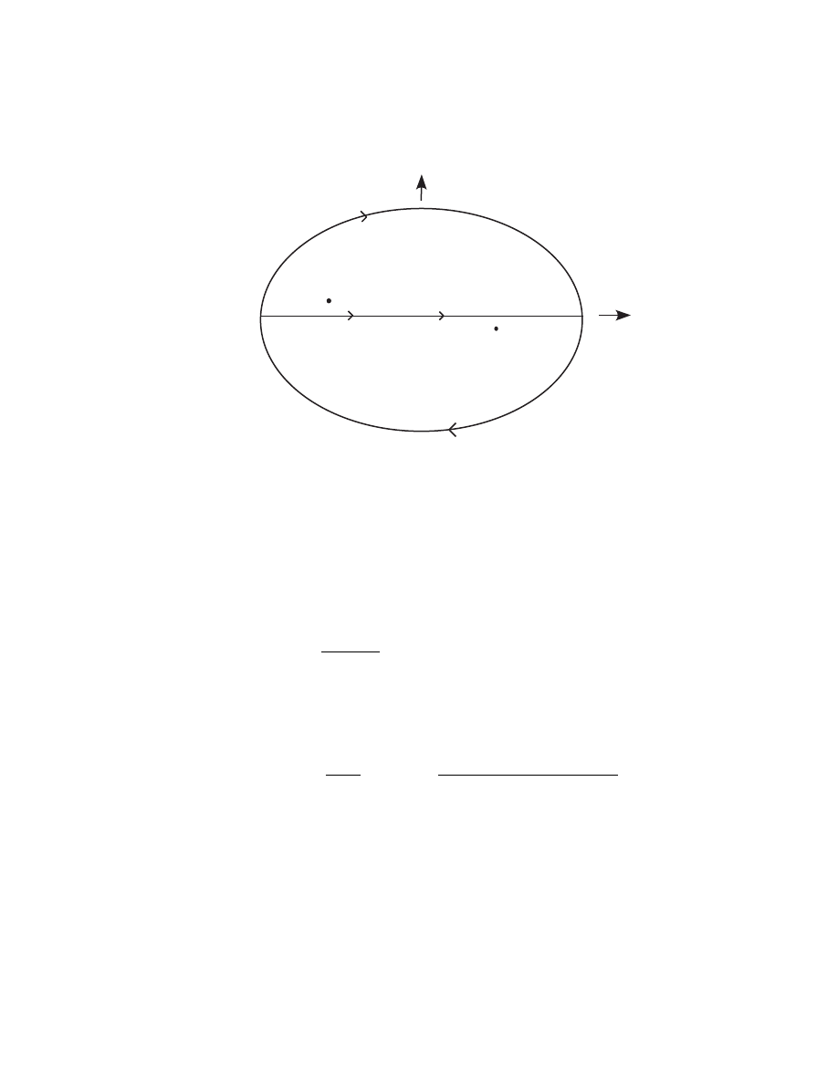
32CHAPTER 2. SECOND QUANTIZATION AND RELATIVISTIC FIELDS
Im k
0
Re k
0
t<0
t>0
k
0
=
ω
0
-i
ε
k
0
=-
ω
0
+
i
ε
Figure 2.1: The complex k
0
plane
We know that this will be a function of x−y, so we can make the algebra
a bit simpler by setting y = 0. Just remember to replace x → x − y at the
end of the calculation. Substituting the fields from (2.97) into (2.105) and
taking the vacuum expectation value gives
iD(x) = h0|T [ ˆ
ϕ(x, t) ˆ
ϕ(0, 0)]|0i
=
Z
d
3
k
(2π)
3
2ω
k
h
θ(t)e
−i(ω
k
t−k·x)
+ θ(−t)e
i(ω
k
t−k·x)
i
(2.109)
Equations (2.108) and (2.109) are really the same result, though this is far
from obvious. In principle, we could derive either form from the other, but
it’s probably easier to start from (2.108).
iD(x) = i
Z
d
3
k
(2π)
4
e
ik·x
Z
dk
0
e
−ik
0
t
(k
0
− ω
k
+ i²)(k
0
+ ω
k
− i²)
(2.110)
Notice how the denominator is factored. Multiplying the two factors and
making the replacements, 2iω
k
² → i² and ²
2
→ 0, gives the same denomina-
tor as (2.108). The dk
0
integration is now performed as a contour integration
in the complex k
0
plane as shown in Figure 2.1. For t < 0 the contour is
completed in the upper half-pane enclosing the point k
0
= −ω
k
+ i², and
for t > 0 the contour is completed in the lower half-plane enclosing the

2.6. THE PROPAGATOR
33
point k
0
= ω − i². The result is identical to (2.109). You see how the i²
in the denominator displaces the poles so as to pick up the right integrand
depending on whether t is positive or negative. Notice finally that (2.106) is
a Lorentz scalar since kx, k
2
and d
4
k are all scalar quantities. You will see
how D(x−y) becomes a key player in perturbation theory via the interaction
picture in the next chapter.

34CHAPTER 2. SECOND QUANTIZATION AND RELATIVISTIC FIELDS

Chapter 3
The Interaction Picture and
the S-Matrix
Most of what we know about subatomic physics comes from two kinds of
experiments: decay experiments and scattering experiments. In a decay
experiment, one starts with some system such as an atom or nucleus or
“elementary” particle and observes the spontaneous transitions that it un-
dergoes. One can determine the lifetime of the system, the identity of the
decay products, the relative frequency of the various decay modes, and the
distribution of momentum and energy among the resulting particles. In a
scattering experiment, one starts with a stable system and bombards it with
another particle. One measures the distribution of momenta among the var-
ious particles produced by the reaction and determines the probability that
the scattering will lead to a particular final state. One common feature of
both these experiments is that the particles are detected when they are not
interacting with one another. They are detected on a scale of distance that
is many orders of magnitude larger than the characteristic de Broglie wave-
length and at times that are vastly longer than the time of interaction. In
non-relativistic quantum mechanics these processes are calculated with first-
order, time dependent perturbation theory using a bit of hocus pocus called
“Fermi’s golden rule.” This is not altogether wrong, but it is inadequate
for several reasons: it can’t accommodate the creation of new particles, it’s
hopelessly non-relativistic, and it only works to first order.
Real scattering theory is difficult. There are many subtle issues involved.
Much of the material in advanced quantum books relates to scattering in one
way or another. I say this because it’s easy to lose sight of the goal amidst all
the technical difficulties. Roughly speaking, there are two basic issues: how
35

36CHAPTER 3. THE INTERACTION PICTURE AND THE S-MATRIX
do the quantum fields ϕ(x) evolve in time, and given this information, how
can we calculate the results of these experiments in terms of the momenta
of particles measured in the asymptotic regime as explained above? The
first question is answered neatly by the interaction picture formalism first
developed by Freeman Dyson. The second question is much more difficult
and will require the remainder of this chapter.
3.1
The Interaction Picture
Path integrals use the Lagrangian; the interaction picture uses the Hamilto-
nian; so I should say a few words about Hamiltonians in general. In classical
mechanics, the two are related by
H = p ˙q − L
(3.1)
In our variety of continuum mechanics the Hamiltonian density becomes
H = π ˙
ϕ − L
(3.2)
For the free Klein-Gordon field
L =
1
2
£
(∂
µ
ϕ)(∂
µ
ϕ) − m
2
ϕ
2
¤
=
1
2
£
˙
ϕ
2
− (∇ϕ)
2
− m
2
ϕ
2
¤
(3.3)
H =
1
2
£
˙
ϕ
2
+ (∇ϕ)
2
+ m
2
ϕ
2
¤
(3.4)
We get the Hamiltonian by integrating (3.4) over all space.
H =
Z
d
3
xH
(3.5)
We assume that the Hamiltonian can be split up into two pieces: H =
H
0
+ H
int
. H
0
is the Hamiltonian of the free field, and H
int
is everything left
over. We assume the H
int
is “small” in some sense; so that the perturbation
series converges. We also have to assume that H
int
is a polynomial of the
fields and their derivatives. The reason for this technical assumption will
appear later.
You will recall the relation between the Schrodinger and Heisenberg pic-
tures is
|ψ(t)i
S
= e
−iHt
|ψi
H
(3.6)
Q
H
(t) = e
iHt
Q
S
e
−iHt

3.1. THE INTERACTION PICTURE
37
This is the usual convention at any rate. |ψi
H
, which does not depend on
time, is a “snapshot” of |ψ(t)i
S
taken at t = 0. This is not necessarily the
most convenient time to take the picture as we will see.
We define the interaction state by
|ψ(t)i
I
≡ e
iH
0
t
|ψ(t)i
S
(3.7)
Q
I
(t) = e
iH
0
t
Q
S
e
−iH
0
t
Some comments:
• It’s clear from (3.6) the Hamiltonian H is the same in the Schrodinger
and Heisenberg pictures, and equally clear from (3.7) that H
0
is the
same in the interaction picture as well. This is not true of the inter-
action piece; since in general, [H
int
, H
0
] 6= 0. I will write
H
I
int
(t) ≡ e
iH
0
t
H
S
int
e
−iH
0
t
(3.8)
Naturally, H
S
int
is the interaction Hamiltonian in the Schrodinger pic-
ture. Notice that H
I
int
(t) depends on time.
• If there were no interactions, |ψ(t)i
I
= |ψi
H
, so the interaction pic-
ture state would be stationary. Now think of a scattering experi-
ment. When the particles are far apart, there is no interaction between
them. In this regime, the interaction picture and Heisenberg pictures
are identical. As the particles begin to interact, H
int
“turns on” and
|ψ(t)i
I
begins to change. Eventually, after the particles are separated
it settles down to a new Heisenberg state.
Actually, this business of “turning on” and “ turning off” skirts a
profound and difficult problem. The trouble is that H
int
never really
turns off. Even when the particles are not interacting with one another,
they are still interacting with themselves by emitting and reabsorbing
virtual particles. Worse yet, even the vacuum interacts with itself by
creating particle-antiparticle pairs. This is a difficult problem, but one
that can be dealt with rigorously.
Define the time evolution operator in the interaction picture, U (t, t
0
), by
|ψ(t)i
I
= U (t, t
0
)|ψ(t
0
)i
I
.
(3.9)
Since H is Hermitian and the norm of |ψi
I
is conserved, we feel entitled by
the rules of quantum mechanics to the following basic relations:
U
†
(t, t
0
)U (t, t
0
) = 1
(3.10)

38CHAPTER 3. THE INTERACTION PICTURE AND THE S-MATRIX
U (t, t) = 1
(3.11)
U (t, t
0
) = U
−1
(t
0
, t)
(3.12)
U (t
2
, t
0
) = U (t
2
, t
1
)U (t
1
, t
0
)
(3.13)
We can derive an equation of motion for U by starting with Schrodinger’s
equation
i
∂
∂t
|ψ(t)i
S
= H|ψ(t)i
S
.
(3.14)
A quick calculation with (3.7) and (3.9) yields
i
∂
∂t
U (t, t
0
) = H
I
int
(t)U (t, t
0
).
(3.15)
We know how to solve equations like this.
U (t, t
0
) = 1 − i
Z
t
t
0
dt
0
H
I
int
(t
0
)U (t
0
, t
0
)
(3.16)
Well – maybe solve is too strong a word, since U appears on both sides of
(3.16). We would like to claim that
U (t, t
0
) = (?) exp
½
−i
Z
t
t
0
dt
0
H
I
int
(t
0
)
¾
This would be the obvious solution if U and H were not operators. The flaw
in the reasoning here is that factors of H
int
don’t commute at different times,
[H
int
(t), H
int
(t
0
)] 6= 0. We can come up with a valid solution by iterating
(3.16) paying careful attention to the time dependence.
U (t, t
0
) = 1 − i
Z
t
t
0
dt
1
H
I
int
(t
1
)
+(−i)
2
Z
t
t
0
dt
1
Z
t
1
t
0
dt
2
H
I
int
(t
1
)H
I
int
(t
2
) + · · ·
(3.17)
The entire series can be summarized by
U (t, t
0
) =
∞
X
n=0
(−i)
n
Z
t
t
0
dt
1
Z
t
1
t
0
dt
2
· · ·
Z
t
n−1
t
0
dt
n
H
I
int
(t
1
)H
I
int
(t
2
) · · · H
I
int
(t
n
)
(3.18)
The series (3.18) is more difficult than it looks. Since the Hamiltonians
don’t commute, we must be meticulously careful to keep later times to

3.2. INTERACTIONS AND THE S MATRIX
39
the left of earlier times. This is called time ordering. We need some
machinery to do this for us. Define the time ordering operator,
T [H(t
1
)H(t
2
)] ≡ H(t
1
)H(t
2
)θ(t
1
− t
2
) + H(t
2
)H(t
1
)θ(t
2
− t
1
)
(3.19)
The generalization to three or more Hamiltonians is obvious. You should
convince yourself that the following things are true:
Z
t
t
0
dt
1
Z
t
1
t
0
dt
2
H(t
1
)H(t
2
) =
Z
t
t
0
dt
2
Z
t
2
t
0
dt
1
H(t
2
)H(t
1
)
=
1
2
Z
t
t
0
Z
t
t
0
dt
1
dt
2
T [H(t
1
)H(t
2
)],
and in general
Z
t
t
0
dt
1
· · ·
Z
t
n−1
t
0
dt
n
H(t
1
) · · · H(t
n
) =
1
n!
Z
t
t
0
dt
1
· · ·
Z
t
t
0
dt
n
T [H(t
1
) · · · H(t
n
)]
So our final result for the U operator is
U (t, t
0
) =
∞
X
n=0
(−i)
n
n!
Z
t
t
0
· · ·
Z
t
t
0
dt
1
dt
2
· · · dt
n
T [H
I
int
(t
1
)H
I
int
(t
2
) · · · H
I
int
(t
n
)],
(3.20)
which can be written in shorthand notation as
U (t, t
0
) = T exp
½
−i
Z
t
t
0
dt
0
H
I
int
(t
0
)
¾
(3.21)
The reason that this is a workable approximation is that the fields that make
up H
I
int
are interaction-picture fields, which according to (3.8), transform as
free fields. Equation (3.20) is a “recipe.” You just insert the formulas for
the free fields and do the algebra.
3.2
Interactions and the S Matrix
A theory with just one kind of particle doesn’t present much opportunity
for interactions. We consider these “toy theories.” We learn to play with
the scattering formalism before we face up to the much greater difficulties
of spin. There are two such models worthy of our attention, the so-called
“phi-cubed” and “phi-to-the-fourth” theories.
H
I
int
=
λ
3!
: ϕ
3
(x) :
(3.22)

40CHAPTER 3. THE INTERACTION PICTURE AND THE S-MATRIX
and
H
I
int
=
λ
4!
: ϕ
4
(x) :
(3.23)
These represent particles interacting with themselves. In (3.22) they interact
in groups of three as you might expect. In (3.23) they interact in groups of
four. As mentioned in Section 2.4, all Hamiltonians must be normal ordered.
Let’s use these to do some sample calculations of scattering precesses. From
a quantum-mechanical perspective, one starts with an initial state consisting
of some particles with well-defined momentum, say |k
1
, k
2
, · · · i prepared in
the lab at a time t → −∞ and observes the probability that this state
evolves to a state hp
1
, p
2
, · · · | as t → +∞. A plausible, though not entirely
correct, way to calculate this is as follows. We start by evaluating (3.21) at
infinite times.
S = T exp
½
−i
Z
∞
−∞
dt
0
H
I
int
(t
0
)
¾
(3.24)
and simply take the expectation value of this operator between free-particle
momentum eigenstates constructed with our creation and destruction oper-
ators. So for example, the two-particle scattering process, k
1
+ k
2
→ p
1
+ p
2
,
would be described by the matrix element
S
βα
= hβ|S|αi
(3.25)
where |αi = a
†
(k
2
)a
†
(k
1
)|0i and hβ| = h0|a(p
1
)a(p
2
). The reason this
is not quite correct is that in addition to interacting with other particles,
particles also interact with themselves, and these self-interactions are partly
responsible for the mass and other physical properties we observe in the
lab. The LSZ reduction scheme to be described later in this chapter deals
with this problem in a systematic way (and leads to simpler calculations
actually) at the expense of adding another conceptual layer of complexity
to the theory. So long as one is working in the approximation that these
self-interactions are ignored (the so-called tree level), the approach described
above is quite satisfactory.
3.2.1
Two-Particle Scattering in the ϕ
4
Theory
The simplest possible scattering process to calculate is k
1
+ k
2
→ p
1
+ p
2
to
lowest order in the ϕ
4
theory. In this case
S = −
iλ
4!
Z
∞
−∞
d
4
x : ϕ
4
(x) :
(3.26)
S
βα
= h0|a(p
1
)a(p
2
)Sa
†
(k
1
)a
†
(k
2
)|0i
(3.27)

3.2. INTERACTIONS AND THE S MATRIX
41
Since : ϕ
4
: is already normal-ordered, there is no time ordering to be done.
If we write ϕ = ϕ
+
+ ϕ
−
where ϕ
+
is the positive frequency part with
annihilation operators and ϕ
−
is the negative frequency part with creation
operators, normal ordering implies that all ϕ
−
’s stand to the left of all
ϕ
+
’s. Only those terms with two creation operators and two annihilation
operators will give a non-zero result when sandwiched between the initial
and final states. The expression : (ϕ
+
+ ϕ
−
)
4
: contains six such terms. A
simple calculation (to be done as an exercise) gives
[ϕ
†
(x)]
2
|k
1
k
2
i =
2e
−i(k
1
+k
2
)x
p
2ω
k
1
2ω
k
2
(2π)
6
|0i
(3.28)
hp
1
p
2
|[ϕ
−
(x)]
2
=
2e
+i(p
1
+p
2
)x
p
2ω
p
1
2ω
p
2
(2π)
6
h0|
where
kx = ωt − k · x
ω =
p
m
2
+ k
2
(3.29)
hp
1
p
2
| : ϕ
4
(x) : |k
1
k
2
i = 6 × 2 × 2
Y
i
1
p
2ω
i
(2π)
3
e
−i(k
1
+k
2
−p
1
−p
2
)x
(3.30)
S
βα
= −iλ
Y
i
1
p
2ω
i
(2π)
3
(2π)
4
δ
(4)
(k
1
+ k
2
− p
1
− p
2
)
(3.31)
The index i on the product sign refers to the momenta, k
1
, k
2
, p
1
, and p
2
.
Notice that the 4! in the denominator of (3.23) cancels the other numerical
factors that appeared in the course of the calculation. It was put there for
that purpose.
The result is surprisingly simple and easy to understand. This is a sim-
ple instance of a general principle first discovered by Feynman; S-matrix
elements can be written down without doing any calculations by just follow-
ing a set of simple rules. We will derive the complete set of rules as we go
along. Here I will just indicate the specific rules that (3.31) illustrates. First
draw a picture in which the initial and final particles are represented by lines
labeled with their momenta. The lines can intersect, but each intersection
point must have exactly four lines. The relevant picture is shown in Figure
3.1. The S-matrix will consist of a product of the following terms obtained
from the picture.
• A factor (2π)
4
δ
(4)
(· · · ). The argument of the delta function, here rep-
resented by a row of dots, insures that total four-momenta is conserved.
• A factor of (−iλ) for each vertex.
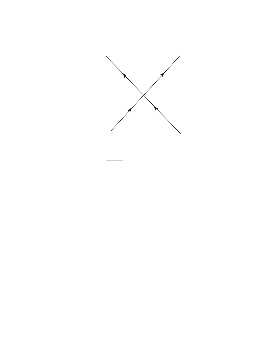
42CHAPTER 3. THE INTERACTION PICTURE AND THE S-MATRIX
k
p
p
k
1
2
1
2
Figure 3.1: The reaction k
1
+ k
2
→ p
1
+ p
2
• A factor 1/
p
2ω
i
(2π)
3
for each of the external momenta. By external
momenta I mean the momenta of particles observed in the initial and
final states. This particular diagram has no internal momenta. We’ll
get to that later.
This particular diagram has only one vertex and one factor of (−iλ)
because we are using the lowest-order term in the perturbation theory ex-
pansion. For the same reason we did not have to deal with the complica-
tions of time ordering. First-order perturbation theory doesn’t cut much
mustard, however. The ϕ
3
theory as well as QED require at least sec-
ond order to calculate anything. We will have to evaluate expressions like
T [: ϕ
4
(x
1
) :: ϕ
4
(x
2
) : · · · ]. This is done with the help of Wick’s theorem.
3.3
The Wick Expansion
Suppose we were to calculate the scattering k
1
+ k
2
→ p
1
+ p
2
in ϕ
3
theory
to lowest non-trivial order perturbation theory. The Feynman diagrams
now have three particles meeting at each vertex, so it requires at least two
vertices to scatter anything. We will have to evaluate the time-ordered
product T [: ϕ
3
(x
1
) :: ϕ(x
2
) :]. To do this by brute force we would split ϕ as
before ϕ = ϕ
−
+ ϕ
+
, and then rearrange the terms to that all ϕ
−
’s stood
to the left of all ϕ
+
’s. There would be 2
6
= 64 terms, so this is already

3.3. THE WICK EXPANSION
43
a formidable calculation. Fortunately there is a theorem from G. C. Wick
that makes it possible to do this calculation without much work.
Take a look at the derivation of the propagator at the end of Chapter 2
h0|T [ϕ
I
(x
1
)ϕ
I
(x
2
)]|0i = iD(x
1
− x
2
)
(3.32)
I am going to describe the steps that led from (2.105) to (2.108) in rather
formal terms that make it easy to generalize to situations in which there are
more than two fields. In order to keep the notation under control, I will write
ϕ(x) = ϕ
+
(x) + ϕ
−
(x), where ϕ
+
is the positive-energy piece containing an
annihilation operator, and ϕ
−
is the negative-energy term with the creation
operator.
• Multiply the fields together with the time-ordering θ functions. This
gives eight terms, each one containing a product of two of the creation
and/or annihilation operators.
T [ϕ(x
1
)ϕ(x
2
)] = (ϕ
+
(x
1
) + ϕ
−
(x
1
))(ϕ
+
(x
2
) + ϕ
−
(x
2
))θ(t
1
− t
2
)
+ (ϕ
+
(x
2
) + ϕ
−
(x
2
))(ϕ
+
(x
1
) + ϕ
−
(x
1
))θ(t
2
− t
1
)
(3.33)
• Use the commutation relations (2.98) to rewrite each term (if neces-
sary) in such a way that all creation operators stand to the left
of all annihilation operators. This is called normal ordering. The
usual notation for this is to enclose the expression between colons, i.e.
: ϕ(x
1
)ϕ(x
2
) : means that the terms between the colons have already
been placed in normal order. In the course of normal ordering there
will appear terms without operators since, for example
ϕ
+
(x
1
)ϕ
−
(x
2
) =: ϕ
−
(x
2
)ϕ
+
(x
1
) : +
Z
d
3
k
(2π)
3
2ω
e
−ik(x
1
−x
2
)
(3.34)
The first term on the right is normal ordered. The second term is a
c-number. Combining all eight terms like this gives
T [ϕ(x
1
)ϕ(x
2
)] =: ϕ(x
1
)ϕ(x
2
) : +iD(x
1
− x
2
)
(3.35)
• The vacuum expectation value of any normal ordered product is zero.
As a consequence
h0|T [ϕ(x
1
)ϕ(x
2
)]|0i = h0| : ϕ(x
1
)ϕ(x
2
) : |0i + iD(x
1
− x
2
)
(3.36)

44CHAPTER 3. THE INTERACTION PICTURE AND THE S-MATRIX
Of course, the first term on the right is zero. We say that iD(x
1
−x
2
) is
the contraction of ϕ(x
1
) and ϕ(x
2
). I will use the overbrace to indicate
contraction. In this notation (3.35) is
T [ϕ(x
1
)ϕ(x
2
)] =: ϕ(x
1
)ϕ(x
2
) : +
z
}|
{
ϕ(x
1
)ϕ(x
2
)
(3.37)
I am now in a position to state Wick’s theorem. The time ordered
product of n fields T [ϕ(x
1
)ϕ(x
2
) · · · ϕ(x
n
)] can be written as a sum of terms
as follows:
• A single term in which all n fields are normal-ordered.
• A sum of terms, each one of which consists of one pair of contracted
ϕ’s. The n − 2 remaining fields are normal-ordered. There is one term
in the sum for each possible pairing of two of the fields.
• A sum of terms, each one of which consists of two pairs of contracted
ϕ’s. The remaining n − 4 remaining fields are normal-ordered. There
is one term in the sum for each way in which two distinct pairs can be
made out of n fields.
• You see the pattern? One term with no contractions plus all possible
terms with one contraction plus all possible terms with two contrac-
tions plus all possible terms with three contractions and so forth. If
n is even, repeat this procedure n/2 times. The last group of terms
will consist of n/2 contractions. There will be one term in this group
for each way of choosing n/2 pairs out of n objects. If n is odd, re-
peat this procedure (n − 1)/2 times. The last terms will have one
normal-ordered field left over
This is all much easier to understand that to explain. The following
example with n = 4 should make this clear.
T [ϕ(x
1
)ϕ(x
2
)ϕ(x
3
)ϕ(x
4
)] =: ϕ(x
1
)ϕ(x
2
)ϕ(x
3
)ϕ(x
4
) :
+
z
}|
{
ϕ(x
1
)ϕ(x
2
) : ϕ(x
3
)ϕ(x
4
) : +
z
}|
{
ϕ(x
1
)ϕ(x
3
) : ϕ(x
2
)ϕ(x
4
) :
+
z
}|
{
ϕ(x
1
)ϕ(x
4
) : ϕ(x
2
)ϕ(x
3
) : +
z
}|
{
ϕ(x
2
)ϕ(x
3
) : ϕ(x
1
)ϕ(x
4
) :
+
z
}|
{
ϕ(x
2
)ϕ(x
4
) : ϕ(x
1
)ϕ(x
3
) : +
z
}|
{
ϕ(x
3
)ϕ(x
4
) : ϕ(x
1
)ϕ(x
2
) :
+
z
}|
{
ϕ(x
1
)ϕ(x
2
)
z
}|
{
ϕ(x
3
)ϕ(x
4
) +
z
}|
{
ϕ(x
1
)ϕ(x
3
)
z
}|
{
ϕ(x
2
)ϕ(x
4
)
+
z
}|
{
ϕ(x
1
)ϕ(x
4
)
z
}|
{
ϕ(x
2
)ϕ(x
3
)
(3.38)

3.4. NEW EXAMPLE – ϕ
3
THEORY
45
You should try working out one of these time ordered products by brute force
starting with (2.97) and (2.98). You will be convinced that the theorem is
true. The proof is more work that it’s worth.
1
3.4
New Example – ϕ
3
Theory
Let’s redo our elastic, two-particle scattering problem with the Hamiltonian
(3.22). To lowest non-zero order of the perturbation expansion
S =
(−i)
2
2!
µ
λ
3!
¶
2
Z
d
4
x
1
Z
d
4
x
2
T [: ϕ
3
(x
1
) :: ϕ
3
(x
2
) :]
(3.39)
We need to calculate S
βα
from (3.27), consequently the only non-vanishing
terms in the Wick expansion are those with four normally-ordered fields and
one pair of contracted fields. There are nine ways of contracting two groups
of three fields. Consequently
T [: ϕ
3
(x
1
) :: ϕ
3
(x
2
) :] = 9
z
}|
{
ϕ(x
1
)ϕ(x
2
) : ϕ
2
(x
1
)ϕ
2
(x
2
) : + · · ·
(3.40)
S
βα
=hp
1
p
2
|S|k
1
k
2
i =
(−i)
2
2!
µ
λ
3!
¶
2
Z
d
4
x
1
Z
d
4
x
2
× 9 ϕ(x
1
)ϕ(x
2
)hp
1
p
2
| : ϕ
2
(x
1
)ϕ
2
(x
2
) : |k
1
k
2
i
(3.41)
A straightforward if time-consuming calculation yields
hp
1
p
2
| : ϕ
2
(x
1
)ϕ
2
(x
2
) : |k
1
k
2
i = 4
Y
i
1
p
2ω
i
(2π)
3
(3.42)
×
n
exp[−i(k
1
+ k
2
)x
2
+ i(p
1
+ p
2
)x
1
] + exp[−i(k
1
+ k
2
)x
1
+ i(p
1
+ p
2
)x
2
]
+ exp[−i(k
1
− p
2
)x
1
+ i(p
1
− k
2
)x
2
] + exp[−i(k
1
− p
1
)x
1
+ i(p
2
− k
2
)x
2
]
+ exp[−i(k
2
− p
2
)x
1
+ i(p
1
− k
1
)x
2
] + exp[−i(k
2
− p
1
)x
1
+ i(p
2
− k
1
)x
2
]
o
Our strategy will be to combine (3.41) and (3.42) and do the integrals over
d
4
x
1
and d
4
x
2
. This will give six terms which collapse into three after a
bit of algebra. The result is rather simple, so let’s just look at the integrals
1
If you want a proof see J. D. Bjorken and S. D. Drell, Relativistic quantum Fields,
Section 17.4

46CHAPTER 3. THE INTERACTION PICTURE AND THE S-MATRIX
over the first term in (3.42). First I need to remind you of some definitions.
From (2.108),
z
}|
{
ϕ(x
1
)ϕ(x
2
) =iD(x
1
− x
2
) = i
Z
d
4
x
(2π)
4
e
−ik(x
1
−x
2
)
k
2
− m
2
+ i²
≡ i
Z
d
4
x
(2π)
4
e
−ik(x
1
−x
2
)
∆
F
(k)
(3.43)
The last line implicitly defines the Feynman propagator,
∆
F
(k) ≡
1
k
2
− m
2
− i²
(3.44)
Notice that ∆
F
(k) = ∆
F
(−k). Now substitute (3.40), (3.42), and (3.43) into
(3.41). Do the integrals, all of which are trivial, starting with the integrals
over d
4
x. The result is
S
βα
=(−iλ)
2
Y
i
1
p
2ω
i
(2π)
3
(2π)
4
δ
(4)
(k
1
+ k
2
− p
1
− p
2
)
× [i∆
F
(k
1
− p
1
) + i∆
F
(k
1
+ k
2
) + i∆
F
(k
1
− p
2
)]
(3.45)
Compare this with the example (3.31). The new feature is the Feynman
propagators. Their role is easy to understand as I will explain in the next
section.
3.5
Feynman Diagrams
Perturbation theory is hard because of all the algebra. The example I have
just worked is the second-easiest scattering problem in QFT, but (3.42),
even with the help of Wick’s theorem, took me nine pages of scratch paper.
And yet, the final answer (3.45) is very simple, and as we will see, can be
represented by three simple diagrams. Feynman diagrams, whatever else
they may be, are part of a “cookbook” recipe for calculating scattering am-
plitudes. You draw some diagrams according to a precise set of topological
rules. Each diagram corresponds to one term in the perturbation-theory
expansion of the scattering amplitude. Each feature of the diagram con-
tributes a specific factor to the term. Once you are in possession of the
rules, you can calculate things like (3.45) without any thought whatsoever.
Here then are (most of) the rules.
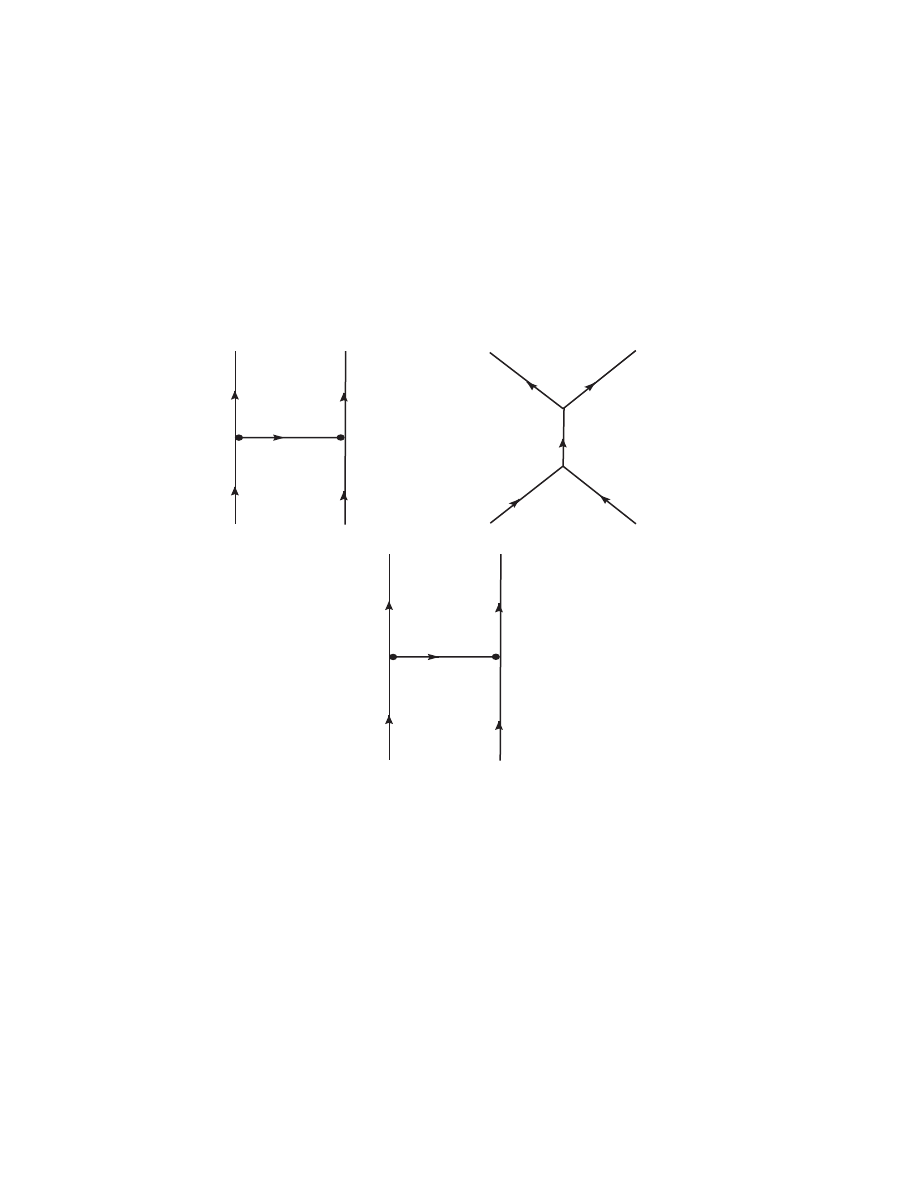
3.5. FEYNMAN DIAGRAMS
47
k
1
k
2
p
1
p
2
k
1
-p
1
k
1
k
2
p
1
p
2
k
1
+k
2
k
1
k
2
p
2
p
1
k
1
-p
2
(a)
(b)
(c)
Figure 3.2: The reaction k
1
+ k
2
→ p
1
+ p
2

48CHAPTER 3. THE INTERACTION PICTURE AND THE S-MATRIX
• The diagrams consist of lines that intersect at points called vertices.
The number of lines (and the identity of the corresponding particles)
depend on the structure of the interaction Hamiltonian. Four lines
meet at each vertex in the ϕ
4
theory and three in the ϕ
3
theory. Dia-
grams arising from the n’th-order terms in the perturbation expansion
have n vertices. For each vertex there is a factor of (−iλ) in the cor-
responding term.
• The lines representing the initial- and final-state particles are called
“external” lines. Each external line contributes a factor 1/
p
2ω
i
(2π)
3
to the amplitude. I always draw the diagrams so that the lines rep-
resenting initial-state particles enter the diagram from below and the
final-state lines leave from above. The diagram represents a sequence
of events in which “time runs up.” Not all authors use the same con-
vention, and it’s important to be consistent. I also put arrows on the
lines indicating the flow of momentum. Although this has not been
relevant so far, lines representing antiparticles carry arrows that point
in the opposite direction to the flow of momentum.
• Suppose you are doing the n-th order term in the perturbation ex-
pansion. Draw all topologically distinct diagrams with n vertices con-
nected by the prerequisite number of lines and with the external lines
entering and leaving the diagram appropriately. In addition to the
external lines that begin or terminate at a vertex, there will be lines
that connect two vertices. These are called internal lines.
• Label all lines with their momentum. External lines carry the momen-
tum that is observed in the lab; in the previous example, k
1
, k
2
, p
1
,
and p
2
. Label the internal lines as you wish, perhaps q
1
, q
2
, q
3
· · ·
would be a good choice. Put an arrow on each of the internal lines
indicating the flow of momentum. The direction you choose will be
arbitrary, but you must make a choice. Momentum is conserved at
each vertex, i.e. the total momentum flowing in (according to the ar-
rows you have just assigned) equals the total momentum flowing out.
If there are no loops all the internal momenta are determined uniquely
by the external momenta. Diagrams without loops are called tree di-
agrams. Life is simple in the trees. For every loop, however, there is
an integral over an undetermined momentum. These integrals usually
diverge and are generally deep trouble. We’ll get to them in the next
chapter.

3.6. THE PROBLEM OF SELF INTERACTIONS
49
• For each internal line with momentum q there is a corresponding factor
of i∆
F
(q) in the scattering amplitude.
• There is an all-over factor of (2π)
4
δ
(4)
(
P
k
i
−
P
p
j
) enforcing conser-
vation of total four-momentum.
• Not all diagrams are relevant. For example, if one or more of the
external lines don’t interact with other particles the diagram represents
a process in which you are probably not interested. There are other
issues that will be discussed later.
• There is one last point that cannot be decreed automatically with
rules. In each calculation there will be a number of combinatorial
factors such as the 9 in (3.40) and the 4 in (3.42). In this particular
calculation they all canceled out, but you can’t count on it in general.
The LSZ reduction scheme in the next section is a big help in deciding
what these factors are.
The rules are easier to understand than to explain. Just look at the
diagrams in Figure 3.2. If I tell you that we are doing second-order two-
particle scattering in ϕ
3
theory, then there are only three possible diagrams
consistent with the rules above, and these are those! You are invited to
review the rules and see how they apply to each of the diagrams and how
they lead to the formula (3.45).
3.6
The Problem of Self Interactions
We can imagine quantum scattering as taking place in three phases. In the
limit t → −∞ the particles are separated and not interacting with one an-
other. As the particles approach one another, the interaction between them
“turns on” as they exchange virtual particles. At some later time t → +∞,
this interaction turns off and they again become free particles. This is diffi-
cult to treat theoretically, since the interaction Hamiltonian itself in no way
turns on or off. So far as theoretical difficulties are concerned, this is only
the tip of the iceberg. As soon as we allow particles to interact with other
particles, they inevitably interact with themselves. When this happens, the
notions of free particles, charge, and vacuum become profoundly subtle.
From the point of view of theory, a free particle is a boiling stream of
self-interactions. From the point of view of experiment, every electron in
the universe is an unremarkable little thing with a well-defined mass, spin,
charge, and magnetic moment. These two views can exist simultaneously

50CHAPTER 3. THE INTERACTION PICTURE AND THE S-MATRIX
because the self-interactions are virtual processes, and as such they are con-
tained within a region roughly the size of the Compton wavelength. So long
as one does not probe inside this region, the electron has it’s usual phys-
ical properties, and probing inside the region means doing a high-energy
scattering experiment.
The same sort of ambiguities also complicate our understanding of the
vacuum state. According to perturbation theory, virtual particle-antiparticle
pairs are spontaneously emitted from and reabsorbed into empty space. This
fact is established experimentally (to some extent) by an experiment measur-
ing the so-called Casimir effect,
2
but apart from this, these vacuum fluctua-
tions have very little consequence, and at any rate, are not well understood.
3
Finally consider the charge of an electron (or more generally, the cou-
pling constant for any sort of interaction). The charge is the measure of
the strength with which photons couple to electrons, but this can only be
measured by doing a scattering experiment, and the experiment must be
interpreted in light of the virtual processes involved.
We believe that all these problems can be addressed, at least for quantum
electrodynamics, but this is a long story, which will occupy us for the next
few chapters. For the time being, let us say that the theory recognizes two
kinds of mass and two kinds of charge. There are the physical or “dressed”
masses and coupling constants – those that are measured in the lab – and
the “bare” masses and coupling constants, which are the parameters that go
into the interaction Lagrangians and Hamiltonians. Somehow the effect of all
virtual processes formulated in terms of the bare particles is to produce the
physical particles. What then are the numerical values of these bare masses
and charges? Alas, we do not know. There is no way to measure them
directly. They could be calculated in principle, but every such calculation
yields infinity! Despite this, we are able to calculate everything that can be
measured (except mass and charge, of course) using only the physical mass
and charge. The fact that we have learned to skirt infinities so violent as to
give sci-fi fans nightmares, is one of the ironic triumphs of modern physics.
In view of this, the interaction picture formulation in the previous section
is a bit too naive. What masses are we to put in H
int
, the bare or the physical
mass? It seems that either way we are stuck. We need to back up and look
at the basic description of scattering processes.
Consider the state of a scattering experiment before the particles have
2
Two charged plates suspended parallel to one another in vacuum experience a very
small repulsive force because of virtual electron-positron pairs created between them.
3
One can calculate the gravitational mass of all the virtual particle-antiparticle pairs
in the universe. The result come out too large by many orders of magnitude.

3.6. THE PROBLEM OF SELF INTERACTIONS
51
interacted. For mathematical purposes we say this corresponds to a time
“t → −∞” (The actual time for a relativistic particle could be as small
as t → −10
−23
seconds.) At this time the particles are free in the sense
explained above. It is customary to call such states “in states,” and write
them |α, ini. The symbol α stands for all the quantum numbers required
to completely specify the state. We will be particularly concerned with
the momentum. If there are n particles in the initial state, we can write
|k
1
, k
2
, . . . , k
n
, ini. The field operators introduced in the previous chapter
can be written
ϕ
in
(x) =
Z
d
3
x
p
2E
k
(2π)
3
h
a
in
(k)e
−ikx
+ a
†
in
(k)e
ikx
i
(3.46)
It is understood that in calculating with this expression, one uses the phys-
ical mass of the particle. In the same way, one defines “out states” hβ, out|,
“out fields” ϕ
out
(x), and “out” creation operators a
†
out
(k) corresponding to
the limit t → ∞. A scattering experiment can be idealized as follows. The
initial target and beam particles are prepared so that they are in a unique
eigenstate of all the relevant operators. We call this state |α, ini. The detec-
tors of the scattered particles are so refined that they can specify that the
final state was in the exact eigenstate hβ, out|. The object of the experiment
is to find what fraction of particles in |α, ini make the transition to hβ, out|.
In other words, we are measuring the probability
P
βα
= |S
βα
|
2
(3.47)
where the so-called S matrix is defined by
S
βα
= hβ, out|α, ini
(3.48)
If we assume that the in states and out states are both complete sets, there
must be some operator S that transforms in states into out states.
hβ, out| = hβ, in|S
(3.49)
S
βα
= hβ, in|S|α, ini
(3.50)
The goal of scattering theory is to calculate the S matrix and the corre-
sponding S operator.
Here are some common-sense properties of S.
1. Nothing in – nothing out, i.e. |S
00
|
2
= 1. Put it another way
h0, in|S = h0, out| = e
iθ
h0, in|
(3.51)

52CHAPTER 3. THE INTERACTION PICTURE AND THE S-MATRIX
The vacuum is stable, but we must allow the possibility that phase of
the vacuum state evolves with time.
2. One-particle states are also stable.
hp, out|p, ini = hp, in|S|p, ini = hp, in|p, ini = 1
(3.52)
3.
ϕ
in
= Sϕ
out
S
−1
(3.53)
Proof:
hβ, out|ϕ
out
|α, ini = hβ, in|Sϕ
out
|α, ini
But hβ, in|ϕ
out
is itself an in state, so we can write
hβ, in|ϕ
out
|α, ini = hβ, out|ϕ
in
S|α, ini
Comparing these two equations gives
Sϕ
out
= ϕ
in
S
4. S is unitary.
Proof:
hβ, in|S = hβ, out|
S
†
|α, ini = |α, outi
hβ, in|SS
†
|α, ini = hα, out|β, outi = S
βα
3.7
The LSZ Reduction Scheme
What is the relation between the fully-interacting field ϕ and ϕ
in
? The
natural guess is
lim
t→−∞
ϕ(x) = ϕ
in
(x)
lim
t→∞
ϕ(x) = ϕ
out
(x)
On second thought though, this can’t be right. The complete field ϕ(x)
is capable of creating states out of the vacuum with two or more virtual
particles. A more careful analysis suggests
lim
t→−∞
ϕ(x) =
√
Z ϕ
in
lim
t→∞
ϕ(x) =
√
Z ϕ
out
(3.54)

3.7. THE LSZ REDUCTION SCHEME
53
Z is understood as the probability for ϕ(x) to produce a single-particle state
out of the vacuum. Even this is not quite correct as an operator equation for
some subtle mathematical reasons that are discussed in the original article.
4
It is correct in terms of matrix elements, for example
lim
t→−∞
hα|ϕ(x)|βi =
√
Zhα|ϕ
in
(x)|βi
where hα| and |βi are arbitrary states. Since we are only interested in
matrix elements in the long run, we will assume (3.54) without any further
comment. Furthermore, the processes in which ϕ(x) produces multiparticle
states out of the vacuum only occur in higher orders of perturbation theory.
When we are working to lowest non-trivial order we can (and will) set Z = 1.
Now we have the apparatus at hand for defining and studying the S
matrix defined in (3.48). We start from an initial state of a system with n
noninteracting physical particles, denoted by
|k
1
· · · k
n
ini = |α ini,
(3.55)
and a final state in which m particles emerge denoted by
hp
1
· · · p
m
out| = hβ out|
(3.56)
Our agenda is to convert (3.48) into an expression involving vacuum expec-
tation values of interacting fields. This is the LSZ reduction technique.
Let us write the in-field in a way analogous to (2.97)
ϕ
in
(x) =
Z
d
3
k
h
f
k
(x)a
in
(k) + f
∗
k
(x)a
†
in
(k)
i
(3.57)
where
f
k
(x) =
e
−ikx
p
(2π)
3
2ω
k
(3.58)
Equation (3.57) can be inverted to yield
a
in
(k) = i
Z
d
3
x f
∗
k
(x)
↔
∂
0
ϕ
in
(x)
a
†
in
(k) = −i
Z
d
3
x f
k
(x)
↔
∂
0
ϕ
in
(x)
(3.59)
4
See also Quantum Theory of Point Particles and Strings, Brian Hatfield, Chapter 7.

54CHAPTER 3. THE INTERACTION PICTURE AND THE S-MATRIX
The notation a
↔
∂
0
b means a∂
0
b − (∂
0
a)b. Since the in-state in (3.48) |α ini
is made up with a product of creation operators as in (3.27), we can write
S
βα
= hβ out|a
†
in
(k)|α − k ini
(3.60)
where |α − k ini represents the initial assemblage of particles represented
by α with one particle of momentum k removed. The procedure is now to
use (3.59) to replace a
†
in
(k) with an integral over ϕ
in
(x). The procedure is
then repeated until all the particles have been removed from the in- and
out- states leaving the vacuum expectation value of the fields.
S
βα
= hβ out|a
†
out
(k)|α − k ini
(3.61)
+hβ out|
h
a
†
in
(k) − a
†
out
(k)
i
|α − k ini
= hβ−k out|α−k ini−ihβ out|
·Z
d
3
x f
k
(x)
↔
∂
0
(ϕ
in
(x) − ϕ
out
(x))
¸
|α − k ini
I have added and subtracted a
†
out
(k) and used (3.59) to eliminate a
†
in
and
a
†
out
. The first term in the last line vanishes unless the initial and final
states are identical. This is the unscattered wave, which we will neglect for
the time being. Now use (3.54) to replace the in- and out- fields with the
complete interacting field. The scattered part can be written as follows:
S
βα
∼
i
√
Z
µ
lim
x
0
→∞
− lim
x
0
→−∞
¶ Z
d
3
x f
k
(x)
↔
∂
0
hβ out|ϕ(x)|α − k ini (3.62)
(The symbol ∼ means that I have temporarily neglected the forward scat-
tering term.) The limits have a nasty non-covariant look about them. I will
clean up the expression with a series of elegant mathematical tricks. For
any two functions such as f
k
(x) and ϕ(x),
µ
lim
x
0
→∞
− lim
x
0
→−∞
¶ Z
d
3
x f
k
↔
∂
0
ϕ =
Z
∞
−∞
d
4
x ∂
0
·
f
k
↔
∂
0
ϕ
¸
=
Z
∞
−∞
d
4
x
·
f
k
∂
2
∂x
2
0
ϕ − ϕ
∂
2
∂x
2
0
f
k
¸
(3.63)
The fact that f
k
satisfies the Klein-Gordon equation allows us to write
ϕ
∂
2
∂x
2
0
f = ϕ(∇
2
− m
2
)f → f (∇
2
− m
2
)ϕ
(3.64)

3.7. THE LSZ REDUCTION SCHEME
55
The sense of the right arrow is that the subsequent expression is obtained
by integrating by parts twice and discarding the surface terms. Finally
substituting (3.63) and (3.64) into (3.62) gives the final result
S
βα
= hβ out|in αi = hβ − k out|α − k ini
(3.65)
+
i
√
Z
Z
d
4
x f
k
(x)(2 + m
2
)hβ out|ϕ(x)|α − k ini
You see the pattern? We have “reduced” an asymptotic particle from the in-
state and replaced it with an interacting field ϕ(x). The price we pay for this
is an integral, a wave function f
k
(x), and a differential operator (2 + m
2
).
We will eventually Fourier transform this expression, whereupon all these
complications will disappear leaving only the inverse of the momentum space
propagator ∆(k).
As an exercise (I am getting tired of typing) you should take the next
step and reduce a particle of momentum p out of the out-state. Convince
yourself that the result is
S
βα
= hβ − p out|α − k ini
(3.66)
∼
µ
i
√
z
¶
2
Z
d
4
x
Z
d
4
y f
k
(x)f
†
p
(y)(2
x
+ m
2
)(2
y
+ m
2
)
× hβ − p, out|T [ϕ(x)ϕ(y)]|α − k, ini
The ∼ sign again means that we have dropped the forward scattering terms.
The new thing here is the time ordered product. You should do the calcu-
lation carefully to see how this comes about. Now suppose there are m
particles in the initial state and n particles in the final state. Just repeat
this procedure n + m times to get the following result:
S
βα
=hp
1
· · · p
n
out|k
1
· · · k
m
ini
∼
µ
i
√
Z
¶
m+n m
Y
i=1
Z
d
4
x
i
f
k
i
(x
i
)(2
x
i
+ m
2
)
n
Y
j=1
d
4
y
j
f
∗
p
j
(y
j
)(2
y
j
+ m
2
)
× h0|T [ϕ(y
1
) · · · ϕ(y
n
)ϕ(x
1
) · · · ϕ(x
m
)]|0i
(3.67)
Equation (3.67), to quote Bjorken and Dell, “serves as a cornerstone for all
calculation of scattering amplitudes in modern quantum field theory.” (This
was before the days of path integrals.)

56CHAPTER 3. THE INTERACTION PICTURE AND THE S-MATRIX
Feynman rules are usually expressed in momentum space, so introduce
the Fourier transform,
G(x
1
· · · x
m
y
1
· · · y
n
) =
m
Y
i=1
Z
d
4
k
i
e
ik
i
x
i
(2π)
4
n
Y
j=1
Z
d
4
p
j
e
−ip
j
y
j
(2π)
4
˜
G(k
1
· · · k
m
p
1
· · · p
n
)
(3.68)
There is a possible confusion about this equation. Since
G(x
1
· · · x
m
y
1
· · · y
n
) = h0|T [ϕ(y
1
) · · · ϕ(y
n
)ϕ(x
1
) · · · ϕ(x
m
)]|0i
(3.69)
There is no distinction between x’s and y’s, but in (3.68), x’s are clearly
associated with incoming particles, and y’s are associated with outgoing
particles. The point is that G(x
1
· · · x
m
y
1
· · · y
n
) is a “general purpose”
tool that can be used in many situations including those on a quantum-
mechanical time scale in which there is no clear-cut distinction between
past and future. In scattering experiments, on the other hand, past and
future are unambiguous. We therefore associate some coordinates with in-
states and some with out-states. We do this by assigning them to k’s (for
incoming particles) or with p’s (for outgoing particles). In this simple theory
with self-interacting scalar fields, the only difference is the + or − signs in
the exponentials in (3.68), but this is necessary to get the conservation
of momentum right. When there are several different kinds of particles
involved, this choice becomes even more significant. For example, if we were
looking at the process e
+
+ e
−
→ γ + γ, (positron annihilation) we would
need to assign x’s to the electron fields and y’s to the photon fields. After
making this assignment, substitute (3.68) into (3.67) and do the necessary
integrals.
S
βα
=hp
1
· · · p
n
out|k
1
· · · k
m
ini
∼
µ
i
√
Z
¶
m+n m
Y
i=1
1
p
(2π)
3
2E
k
i
(k
2
i
− m
2
)
×
n
Y
j=1
1
q
(2π)
3
2E
p
j
(p
2
j
− m
2
) ˜
G(k
1
· · · k
m
p
1
· · · p
n
)
(3.70)
3.8
Correlation Functions
The heart of (3.67) is the vacuum correlation function
G(x
1
· · · x
n
) = h0|T [ϕ(x
1
)ϕ(x
2
) · · · ϕ(x
n
)]|0i
(3.71)

3.8. CORRELATION FUNCTIONS
57
The fields ϕ(x) are the fully interacting fields in the Heisenberg picture.
If we are to calculate anything in this formalism, we must somehow relate
them to the “in” fields defined in (3.54). Let’s hope there exists an operator
U (t) such that
ϕ(x) = U
−1
(t)ϕ
in
(x)U (t)
with t = x
0
(3.72)
I happen to know that the necessary operator is given by
U (t) = lim
t
0
→−∞
U (t, t
0
)
(3.73)
where U (t, t
0
) is time time-development operator given by (3.21). This is
plausible, but it need to be proved.
Both ϕ and ϕ
in
satisfy Heisenberg equations of motion.
∂
∂t
ϕ(t) = i[H(ϕ), ϕ(t)]
(3.74)
∂
∂t
ϕ
in
(t) = i[H
0
(ϕ
in
), ϕ
in
(t)]
(3.75)
I have written H(ϕ) and H
0
(ϕ
in
) to emphasize that the Hamiltonians are
functionals of their respective fields. I have also written ϕ(t). I realize the
ϕ is really a function of the four vector x
µ
, but I am specifically concerned
with the time development here, and x
0
= t. Note that
d
dt
£
U U
−1
¤
=
dU
dt
U
−1
+ U
dU
−1
dt
= 0
In a condensed notation this is
U ˙
U
−1
= − ˙
U U
−1
(3.76)
Now substitute (3.72) into (3.75) and use (3.74) to eliminate ˙
ϕ.
∂
∂t
ϕ
in
=
∂
∂t
£
U ϕU
−1
¤
= ˙
U ϕU
−1
+ U ˙
ϕU
−1
+ U ϕ ˙
U
−1
= ˙
U (U
−1
ϕ
in
U )U
−1
+ U i [H(ϕ), ϕ] U
−1
+ U (U
−1
ϕ
in
U ) ˙
U
−1
= ˙
U U
−1
ϕ
in
− ϕ
in
˙
U U
−1
+ i
£
(U H(ϕ)U
−1
), U ϕU
−1
¤
=
h
˙
U U
−1
, ϕ
in
i
+ i [H(ϕ
in
), ϕ
in
] = i [H
0
(ϕ
in
), ϕ
in
]
(3.77)

58CHAPTER 3. THE INTERACTION PICTURE AND THE S-MATRIX
I have used (3.76) to simplify the second line of (3.77). I have also used the
fact that Hamiltonians are polynomials of ϕ (and possibly its derivatives),
so for example, U H(ϕ)U
−1
= H(ϕ
in
). Therefore
hn
˙
U U
−1
+ iH
int
(ϕ
in
)
o
, ϕ
in
i
= 0
The operator in curly brackets commutes with all ϕ
in
. It must therefore
be a c number. We could think of this constant as a number added to the
Hamiltonian. We have had several occasions to discard such numbers before
and will do so now. We conclude that (to within a meaningless additive
constant)
i
dU (t)
dt
= H
int
(ϕ
in
)U (t)
(3.78)
This is equation (3.15) with the important clarification that H
int
is con-
structed with in fields, i.e. fields using the physical masses of the particles
involved. We can take U (t, t
0
) to be given by (3.21) and U (t) by (3.73).
Using (3.12) and (3.13) we can argue that
U (t
2
, t
1
) = lim
t→−∞
U (t
2
, t
0
)U (t
0
, t
1
)
= lim
t→−∞
U (t
2
, t
0
)U
−1
(t
1
, t
0
) = U (t
2
)U
−1
(t
1
)
(3.79)
Now consider a set of time-ordered points x
1
, · · · , x
n
satisfying x
1
0
>
x
0
2
> · · · > x
0
n
. Using (3.79) we can write
G(x
1
, · · · , x
n
) = h0|ϕ(x
1
) · · · ϕ(x
n
)|0i
= h0|U (t
0
, t
1
)ϕ
in
(x
1
)U (t
1
, t
2
)ϕ
in
(x
2
) · · · U (t
n−1
, t
n
)ϕ
in
(x
n
)U (t
n
, t
0
)|0i
(3.80)
The sequence of times reading from left to right runs from t
0
→ −∞ to t
1
and back again to −∞. We can deform the contour by writing U (t
0
, t
1
) =
U (t
0
, −t
0
)U (−t
0
, t
1
). An operator of the form U (−t
0
, t
0
) runs from −∞ to
+∞. It has the effect of transforming asymptotic initial states to asymptotic
final states. This is just the role of the S operator defined in (3.74). We will
simply call U (t
0
, −t
0
) = S
−1
. With this change, our correlation function
becomes
G(x
1
, · · · , x
n
)
= h0|S
−1
U (−t
0
, t
1
)ϕ
in
(x
1
)U (t
1
, t
2
) · · · U (t
n−1
, t
n
)ϕ
in
(x
n
)U (t
n
, t
0
)|0i
(3.81)

3.8. CORRELATION FUNCTIONS
59
According to (3.51), the vacuum state is an eigenstate of S with a complex
phase. We can write h0|S
−1
= e
−iθ
h0| and find the phase as follows.
h0|S|0ih0|S
−1
= h0|
The point is that since the vacuum is stable, |0ih0| constitutes a complete
set of states. Consequently
h0|S
−1
=
h0|
h0|S|0i
(3.82)
Equation (3.81) becomes
G(x
1
, · · · , x
n
)
(3.83)
=
h0|U (−t
0
, t
1
)ϕ
in
(x
1
)U (t
1
, t
2
) · · · U (t
n−1
, t
n
)ϕ
in
(x
n
)U (t
n
, t
0
)|0i
h0|S|0i
Consider an operator like U (t
i−1
, t
i
). It contains an infinite sum of prod-
ucts of fields evaluated at various times, but every term in the sum contains
fields that are time-ordered between t
i−1
and t
i
. The entire numerator of
(3.83) consists of a vast array of fields, but they are all time ordered. Of
course, we started out with the assumption that the sequence of coordi-
nates x
1
, x
2
, · · · x
n
was already time ordered, so this makes the “scaffolding”
around which the U ’s are time ordered. The original definition of G, equa-
tion (3.71) already contains the time ordering operator, so we need not have
made that assumption. We just need to write it
G(x
1
, · · · , x
n
)
(3.84)
=
h0|T [U (−t
0
, t
1
)ϕ
in
(x
1
)U (t
1
, t
2
) · · · U (t
n−1
, t
n
)ϕ
in
(x
n
)U (t
n
, t
0
)] |0i
h0|S|0i
With the time-ordering operator in place, we are free to move the factors
around in the numerator to suit our convenience. In particular, we can
gather all the U ’s together.
U (−t
0
, t
1
)U (t
1
, t
2
) · · · U (t
n
, t
0
) = U (−t
0
, t
0
) = S
Our final result for the correlation function function is
G(x
1
, · · · , x
n
) =
h0|T [ϕ
in
(x
1
)ϕ
in
(x
2
) · · · ϕ
in
(x
n
)S] |0i
h0|S|0i
(3.85)

60CHAPTER 3. THE INTERACTION PICTURE AND THE S-MATRIX
Itzykson and Zuber
5
in a masterstroke of French understatement, call
this derivation “heuristic.” The fact is that we just don’t know how to
do rigorous mathematics with such badly-behaved operator expansions as
(3.20), and there are many subtle physical questions as well. You might call
this “experimental mathematics.” We use this formula and it works. It is
also true that equivalent formulas can be derived using the path integral for-
malism. This also goes way beyond the limits of conventional mathematics,
but the same result is obtained in the end.
3.9
Two Examples
Let’s take the interaction Hamiltonian H
int
= (λ/4!)ϕ
4
(x) that we stud-
ied in Sections 4.3 and 4.4, and calculate the four-point Green’s function
G(x
1
, x
2
, x
3
, x
4
) to first order in λ. The S-operator (3.24) to first order is
S = 1 −
iλ
4!
Z
d
4
x : ϕ
4
(x) : + · · ·
(3.86)
Note that to first order h0|S|0i = 1, so (3.85) becomes
G(x
1
, x
2
, x
3
, x
4
) = h0|T [ϕ
in
(x
1
)ϕ
in
(x
2
)ϕ
in
(x
3
)ϕ
in
(x
4
)]|0i
−
iλ
4!
h0|T
·
ϕ
in
(x
1
)ϕ
in
(x
2
)ϕ
in
(x
3
)ϕ
in
(x
4
)
Z
d
4
x : ϕ
4
I
(x) :
¸
|0i + · · ·
(3.87)
The zeroth-order term can be read off of (3.37)
G(x
1
, x
2
)G(x
3
, x
4
) + G(x
1
, x
3
)G(x
2
, x
4
) + G(x
1
, x
4
)G(x
2
, x
3
)
(3.88)
This is the sum of all possible ways two particles can propagate between two
pairs of points. As you would expect in this zeroth-order term, the particles
do not interact .
The first-order term has eight fields each with two terms. If you were to
simply multiply them out there would be 2
8
= 256 terms, so here’s where
Mr. G. C. Wick earns his keep. First notice that the vacuum expectation
value of any normal-ordered product of fields vanishes. We need only be
concerned with terms in which all eight fields are contracted. Because of
the normal-ordered Hamiltonian, we don’t contract the four ϕ(x)’s with one
another. The only surviving terms are those in which each of ϕ(x
1
), ϕ(x
2
),
ϕ(x
3
), and ϕ(x
4
) is contracted with one of the ϕ(x)’s. There are, of course,
5
Quantum Field Theory, C. Itzykson and J.-B. Zuber, McGraw-Hill 1980

3.9. TWO EXAMPLES
61
4! ways of doing this all leading to the same expression for the first-order
contribution to G(x
1
, x
2
, x
3
, x
4
).
G(x
1
, x
2
, x
3
, x
4
) = −iλ
Z
d
4
xG(x
1
, x)G(x
2
, x)G(x
3
, x)G(x
4
, x)
(3.89)
Now suppose you want to calculate the S matrix element for the scatter-
ing of two particles k
1
+ k
2
→ p
1
+ p
2
again to first order. We will use (3.67)
with m = n = 2. To first order there is no renormalization so Z = 1.(More
about this in the next chapter.) We’ll use (3.89) with x
3
set equal to y
1
and
x
4
= y
2
. Take advantage of the fact that G is a Green’s function after all,
so
(2
x
+ m
2
)G(x, x
0
) = i(2
x
+ m
2
)D(x − x
0
) = −iδ
(4)
(x − x
0
)
(3.90)
You see, all the (2
x
i
+ m
2
) operators in (3.67) produce factors of −iδ
(4)
(x
i
−
x) when they operate on G(x
i
, x). Now all the integrals are trivial.
S
βα
=hp
1
p
2
out|k
1
k
2
ini
=(−iλ)(2π)
4
δ
(4)
(p
1
+ p
2
− k
1
− k
2
)
×
2
Y
i=1
1
p
(2π)
3
2E
k
i
2
Y
j=1
1
q
(2π)
3
2E
p
j
,
(3.91)
which is the same result as (3.31) obtained with our more naive approach.
It’s worth noting that the arguments leading up to this result are very subtle,
but the actual calculation is very little effort.
Before leaving this example I should mention the factor h0|S|0i in the
denominator of (3.84). It is an infinite series of terms representing particles
that spring spontaneously out of the vacuum and then disappear back into
the vacuum, vacuum-to-vacuum graphs the’re called. The same graphs ap-
pear in the numerator, but in our simple example, they are all multiplied by
the S-matrix for k
1
+k
2
→ p
1
+p
2
. If we carried out the calculation to infinite
order, all the vacuum-to-vacuum graphs in the denominator would cancel
those in the numerator leaving an infinite series for k
1
+k
2
→ p
1
+p
2
without
any “disconnected” graphs. We are thus entitled to ignore the denominator
so long as we remember to discard all the multiplicative vacuum-to-vacuum
graphs in the numerator.
Finally let’s work out the S-matrix for k
1
+k
2
→ p
1
+p
2
in the ϕ
3
theory.
The correlation function (3.85) is
G(x
1
, x
2
, y
1
, y
2
) =
1
2!
µ
−iλ
3!
¶
2
Z
d
4
x
Z
d
4
y
×h0|T [ϕ
in
(x
1
)ϕ
in
(x
2
)ϕ
in
(y
1
)ϕ
in
(y
2
) : ϕ
3
I
(x) :: ϕ
3
I
(y) :]|0i
(3.92)

62CHAPTER 3. THE INTERACTION PICTURE AND THE S-MATRIX
Only those terms in the Wick expansion with fully contracted fields will
survive, and only those in which all of the ϕ
in
’s are contracted with the ϕ
I
’s
will be relevant. The surviving terms then are these
h0|T [ϕ
in
(x
1
)ϕ
in
(x
2
)ϕ
in
(y
1
)ϕ
in
(y
2
) : ϕ
3
I
(x) :: ϕ
3
I
(y) :]|0i = · · ·
+
z
}|
{
ϕ
in
(x
1
)ϕ
I
(x)
z
}|
{
ϕ
in
(x
2
)ϕ
I
(y)
z
}|
{
ϕ
in
(y
1
)ϕ
I
(x)
z
}|
{
ϕ
in
(y
2
)ϕ
I
(y)
z
}|
{
ϕ
I
(x)ϕ
I
(y)
+
z
}|
{
ϕ
in
(x
1
)ϕ
I
(x)
z
}|
{
ϕ
in
(x
2
)ϕ
I
(x)
z
}|
{
ϕ
in
(y
1
)ϕ
I
(y)
z
}|
{
ϕ
in
(y
2
)ϕ
I
(y)
z
}|
{
ϕ
I
(x)ϕ
I
(y)
+
z
}|
{
ϕ
in
(x
1
)ϕ
I
(x)
z
}|
{
ϕ
in
(x
2
)ϕ
I
(y)
z
}|
{
ϕ
in
(y
1
)ϕ
I
(y)
z
}|
{
ϕ
in
(y
2
)ϕ
I
(x)
z
}|
{
ϕ
I
(x)ϕ
I
(y)
+ · · ·
(3.93)
and another three terms that are identical except that the x’s and y’s (with-
out subscripts) are interchanged. There are (3!)
2
ways of making each of
these six terms, so all the combinatorial factors cancel. When G from (3.92)
is substituted back into (3.67) all the ϕ
in
’s disappear since for example (see
(3.90))
Z
d
4
x
1
(2
x
1
+ m
2
)
z
}|
{
ϕ
in
(x
1
)ϕ
I
(x) = −i.
(3.94)
When the smoke has cleared the result is the same as (3.45).

Chapter 4
The Trouble with Loops
Suppose we were doing our standard two-body scattering problem to fourth
order in ϕ
3
theory. The correlation function is
G(x
1
, x
2
, y
1
, y
2
) =
1
4!
µ
−iλ
3!
¶
4
Z
d
4
w
Z
d
4
x
Z
d
4
y
Z
d
4
z
×h0|ϕ
in
(x
1
)ϕ
in
(x
2
)ϕ
in
(y
1
)ϕ
in
(y
2
) : ϕ
3
(w) :: ϕ
3
(x) :: ϕ
3
(y) :: ϕ
3
(z) : |0i
(4.1)
The Wick expansion will consist of a vast number of terms, but there is one
class of terms that concerns me now.
: ϕ
in
(x
1
)ϕ
in
(x
2
)ϕ
in
(y
1
)ϕ
in
(y
2
) :
z
}|
{
ϕ(w)ϕ(x)
z
}|
{
ϕ(x)ϕ(y)
z
}|
{
ϕ(x)ϕ(y)
z }| {
ϕ(y)ϕ(z)
(4.2)
The associated Feynman diagram is shown in Figure 4.1. Because of con-
servation of momentum at each vertex, p = k
1
− p
1
= p
2
− k
2
. I have also
labeled the loop momentum in such as way as to acknowledge this rule. If
we were to finish the calculation with this diagram and obtain the corre-
sponding term in the S-matrix expansion, it would be identical to the first
term of (3.45) except for the replacement
i∆
F
(p) → i∆
F
(p)
·Z
d
4
q
(2π)
4
(−iλ)i∆
F
(p − q)(−iλ)i∆
F
(q)i∆
F
(p)
¸
(4.3)
There are three points to be made about this. The first is that the integral
over q is ubiquitous whenever there are loops. This is in fact the last of the
Feynman rules for this simple scalar field theory.
63
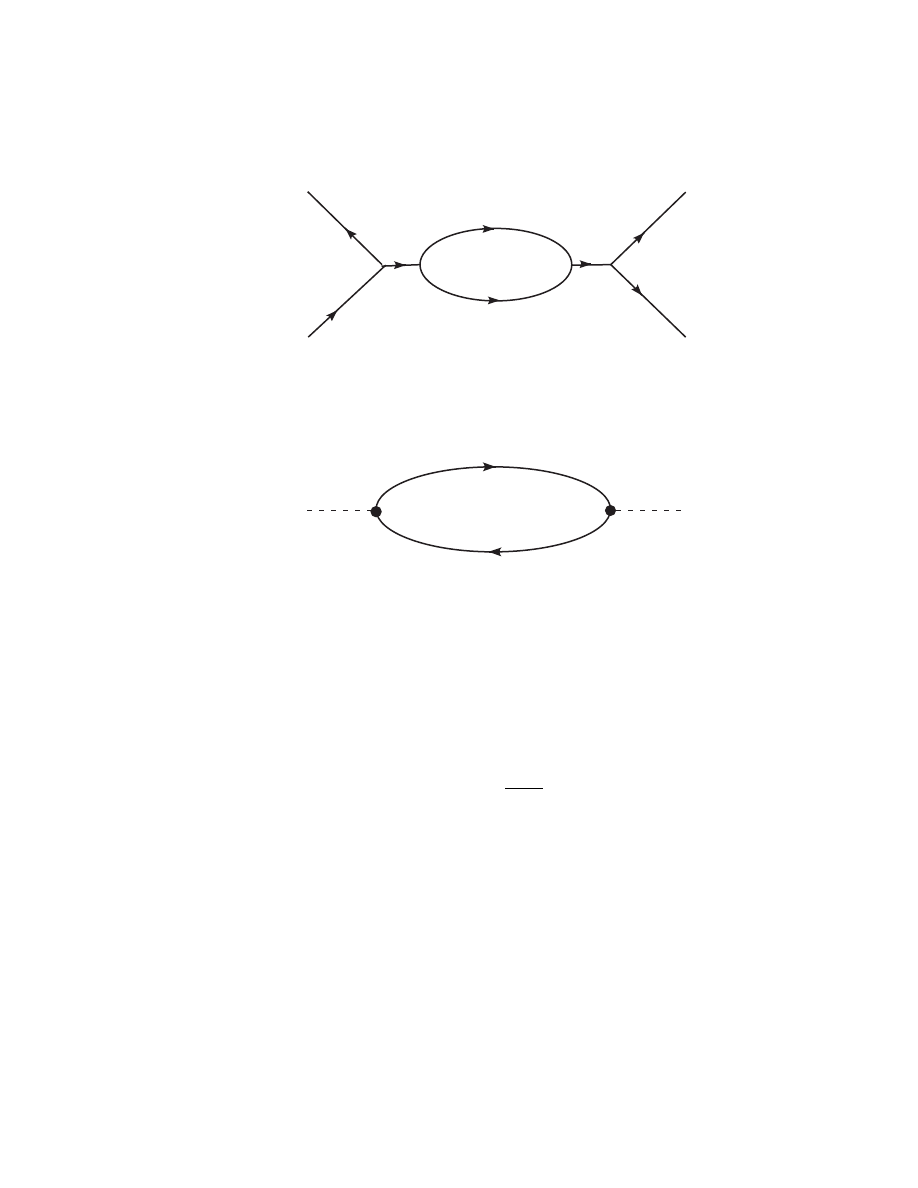
64
CHAPTER 4. THE TROUBLE WITH LOOPS
k
1
p
1
p
2
k
2
p
p
q
p-q
Figure 4.1: The one-loop correction to the propagator.
q
p - q
- i
λ
- i
λ
Figure 4.2: The truncated one-loop diagram.
• For every continuous loop there will be one undetermined momentum
and an integral over it of the form
Z
d
4
q
(2π)
4
.
(4.4)
The second point is that the effect of the loop is to make a multiplicative
correction to the ∆
F
(p) that appeared in second order. The correction factor
is the quantity in the square brackets in (4.3). The correction is proportional
to λ
2
, so if λ is small, whatever that means, the correction itself might be
small. As we explore higher orders in perturbation theory, there will be
two-loop corrections proportional to λ
4
, three-loop corrections proportional
to λ
6
and so forth. If we are lucky the series will converge.

4.1. DOING THE INTEGRALS
65
The third point is that we are not lucky. The integrals are all infinite.
To see why this is so look at the “truncated” diagram Figure 4.2
Z
d
4
q
(2π)
4
(−iλ)i∆
F
(q)(−iλ)i∆
F
(p − q)
= λ
2
Z
d
4
q
(2π)
4
1
q
2
− m
2
+ i²
1
(p − q)
2
− m
2
+ i²
(4.5)
There are four powers of q in the numerator and four in the denominator, so
the integral diverges like
R
dx/x, i.e. logarithmically. Nonetheless, integrals
of this sort can be unambiguously divided into a finite and an infinite part.
We can show that the infinite part affects only the coupling constant λ
and the mass m, whereas the finite part provides a real and measurable
correction to the theory. The purpose of this chapter is to show how this
comes about.
4.1
Doing the Integrals
The integral in (4.5) is typical of loop integrals in general, and over the years
a number of tricks and identities have evolved for doing them. What follows
is a brief primer on these techniques. The first trick is to make the integral
five-dimensional by introducing the Feynman parameter z. You can readily
verify that
1
AB
=
Z
1
0
dz
[Az + B(1 − z)]
2
≡
Z
1
0
dz
D
2
(4.6)
or more generally
1
A
1
A
2
· · · A
n
=
Z
1
0
dz
1
· · · dz
n
δ
³X
z
i
− 1
´
(n − 1)!
[z
1
A
1
+ z
2
A
2
+ · · · + z
n
A
n
]
n
(4.7)
In this case set
A =(p − q)
2
− m
2
+ i²
B = q
2
− m
2
+ i²
D = q
2
− m
2
+ z(p
2
− 2pq) + i²
(4.8)
Now complete the square by setting
` = q − pz
(4.9)
D = `
2
− m
2
+ p
2
z(1 − z) + i² = `
2
− ∆ + i²
(4.10)

66
CHAPTER 4. THE TROUBLE WITH LOOPS
where
∆ ≡ m
2
− p
2
z(1 − z)
(4.11)
Equation (4.5) is now
λ
2
Z
1
0
dz
Z
d
4
`
(2π)
4
1
(`
2
− ∆ + i²)
2
(4.12)
Most loop integrals are done by combining denominators using (4.6) or
(4.7) and then completing the squares as in (4.9) and (4.10). The result is
an integral of the form
Z
d
4
l
(2π)
4
1
(l
2
− ∆ + i²)
n
(4.13)
There is a general procedure for evaluating such integrals which I will now
describe. As it stands this is an integral in Minkowski space. The first step
toward putting it in a manageable form is to convert it to Euclidean space.
We therefore define a Euclidean momentum
`
0
≡ i`
0
E
`
E
= `
(4.14)
Recall from Section 2.6 and particularly equation (2.110) that the dk
0
in-
tegral in the propagator is to be understood as a contour integral in the
complex k
0
plane. The transformation (4.14) amounts to rotating the con-
tour 90
0
counterclockwise. You can see from Figure 2.1 that this is possible
without crossing any poles. This maneuver is called a Wick rotation. The
integral is now
i(−1)
n
Z
d
4
`
E
(2π)
4
1
(`
2
E
+ ∆)
n
=
i(−1)
n
(2π)
4
Z
dΩ
4
Z
∞
0
d`
E
`
3
E
(`
2
E
+ ∆)
n
.
(4.15)
The i² has no further role to play, so I have deleted it. The integral over
dΩ
4
gives the total solid angle in four-dimensional space. There is a simple
formula for the solid angle in any dimension d.
Z
dΩ
d
=
2π
d/2
Γ(d/2)
(4.16)
The Γ function is defined as usual.
Γ(α) =
Z
∞
0
dt t
α−1
e
−t
(4.17)

4.1. DOING THE INTEGRALS
67
with Γ(α + 1) = αΓ(α) and Γ(n) = (n − 1)! for n integer. The derivation of
(4.16) is quite ingenious. I have included it as an appendix to this chapter
so as not to distract from our topic. It’s easy to verify that this gives the
expected results.
R
dΩ
2
= 2π and
R
dΩ
3
= 4π. As it turns out
R
dΩ
4
= 2π
2
,
a result that could have been obtained in other ways as well. The interesting
point, however, is that the right side of (4.16) is perfectly well defined for
non-integer d. Thus we can imagine doing the integral
Z
d
d
`
E
(2π)
d
1
(`
2
E
+ ∆)
2
=
Z
dΩ
d
(2π)
d
·
Z
∞
0
d`
E
`
d−1
E
(`
2
E
+ ∆)
2
(4.18)
using (4.16) for
R
dΩ
d
. As it turns out, the second integral is also doable for
non-integer d. Again the derivation is quite remarkable. I have included a
brief outline of it in the appendix. The final result is
Z
d
d
`
E
(2π)
d
1
(`
2
E
+ ∆)
n
=
1
(4π)
d/2
Γ(n − d/2)
Γ(n)
µ
1
∆
¶
n−d/2
(4.19)
Now if n = 2 and d = 4, Γ(0) = ∞, which tells us what we already knew,
the integral in (4.5) diverges. Of course Γ(x) has poles at zero and negative
integers, but aside from that, it is smooth and well defined. We can get
a finite answer by taking d = 4 − ², where ² is some small positive num-
ber. Figuratively speaking, we are integrating over slightly less than four
dimensions! You will see the point in this in a few lines.
Before finishing the integral, we need one more theorem (see Appendix)
X
²
= 1 + ² ln X + O(²
2
)
(4.20)
and a more or less well known result
Γ(²) =
1
²
− γ + O(²)
(4.21)
where γ is the Euler-Mascheroni constant ≈ 0.5772.
Now using (4.14), (4.19), (4.20) and (4.21), (4.12) becomes
λ
2
Z
1
0
dz
Z
d
d
l
E
(2π)
d
i
(l
2
E
+ ∆)
2
= iλ
2
Z
1
0
dz
1
(4π)
d/2
Γ(2 − d/2)
Γ(2)
µ
1
∆
¶
2−d/2
= iλ
2
Z
1
0
dz
(4π)
2
·
2
²
− γ + ln 4π − ln ∆ + O(²)
¸
(4.22)

68
CHAPTER 4. THE TROUBLE WITH LOOPS
Now here’s the point; it’s still divergent as ² → 0, but so long as we keep
² finite, we can still do rigorous mathematics. Our hope is that when we
put this diagram in context with the rest of the theory, we will arrive at a
point where all the ²-dependent terms cancel out. We can then set ² = 0,
because nothing depends on ².
I should mention that there are at least two other ways to separate out
the divergence. One can simply put a cutoff Λ at some large value of `
2
E
in (4.15) and then investigate the result in the limit Λ → ∞. One can
also modify the propagator so that it goes to zero more rapidly and helps
the convergence of the loop integrals. For instance we could replace the
propagator
1
p
2
− m
2
+ i²
→
1
p
2
− m
2
+ i²
−
1
p
2
− M
2
+ i²
(4.23)
where M À m is the mass of some fictitious particle. For p
2
¿ M
2
the
second propagator is essentially zero, but when p
2
> M
2
the two propagators
partially cancel and the combination falls off like 1/p
4
. We would then take
the limit M → ∞ to separate out the divergence. This is called Pauli-Villars
regularization. All three techniques yield consistent results for our current
problem, but the cutoff method gets into trouble with gauge invariance
where that is an issue, and the Pauli-Villars scheme is “messy” in that it
involves introducing non-existent particles.
So what are we to make of these infinities? Perhaps the theory is some-
how wrong at large momentum transfers. We could decide to live with our
ignorance and regard it as a low-energy approximation to some as yet undis-
covered formalism. There is a more ambitious hope that the shortcomings
of the theory only affect our ability to calculate the mass and coupling con-
stant. The idea here is that the m and λ that appear in the Lagrangian are
not the real physical quantities but rather some “bare” mass and coupling
constant. If all our integrals were finite, then the loop diagrams would mod-
ify the bare quantities. If we knew what to put in the Lagrangian in the first
place and then carried out the perturbation expansion to arbitrarily high
order, we would end up with the laboratory values of m and λ. A theory
with these properties is said to be renormalizable. Our scalar field theories
in fact are. We will explore this in the next section.
Before we do so, however, there are two other diagrams that we must
evaluate. The first, Figure 4.3, is affectionately known as a tadpole diagram.
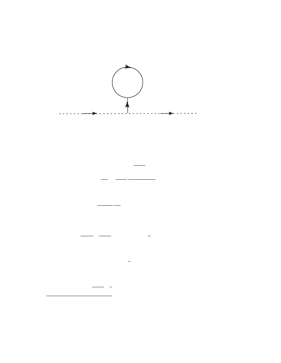
4.1. DOING THE INTEGRALS
69
p
p
q
Figure 4.3: The tadpole correction to the propagator.
Truncating the diagram as in (4.5) leaves the terms
(iλ)i∆
F
(0)(iλ)
Z
d
4
q
(2π)
4
i∆
F
(q
2
)
=
λ
2
m
2
Z
d
4
q
(2π)
4
1
p
2
− m
2
+ i²
(4.24)
We can use (4.19) with ∆ = m
2
and n = 1.
=
−i
(4π)
d/2
λ
2
m
2
Γ(1 − d/2)(m
2
)
d/2−1
(4.25)
Because the integral diverges quadratically, we need to generalize (4.21) a
bit. For x near −n
Γ(x) =
(−1)
n
n!
µ
1
x + n
− γ + 1 + · · · +
1
n
+ O(x + n)
¶
(4.26)
In this case x + 1 = 2 − d/2 ≡ ².
Γ(1 − d/2) = −
µ
1
²
− γ + 1 + O(²)
¶
(4.27)
Our final result for Figure 4.3 is
1
iλ
2
(4π)
2
µ
1
²
− γ − ln(m
2
) + ln(4π)
¶
(4.28)
1
Both (4.28) and (4.22) have the odd feature of a logarithm of a dimensionfull quantity.
The reasons for this are both subtle and important. By insisting that spatial integrals
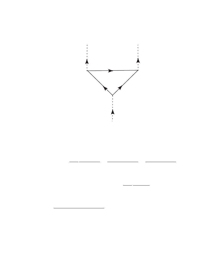
70
CHAPTER 4. THE TROUBLE WITH LOOPS
p
k
p - k
q
q - k
p - q
Figure 4.4: The third-order vertex correction.
The diagram in Figure 4.4 modifies the vertex where three lines meet.
Neglecting the external lines, the triangle part of the diagram is
(iλ)
Z
d
4
q
(2π)
4
i
q
2
− m
2
+ i²
(iλ)
i
(q − k)
2
− m
2
+ i²
(iλ)
i
(p − q)
2
− m
2
+ i²
(4.29)
Combine the denominators using (4.7)
= iλ
3
Z
1
0
dz
2
Z
1
0
dz
3
Z
d
4
`
E
(2π)
4
1
(`
2
E
+ ∆)
3
(4.30)
Where
∆ = (z
2
k + z
3
p)
2
− z
2
k
2
− z
3
p
2
+ m
2
(4.31)
have dimension d 6= 4 we have changed the dimensionality of ϕ and L. In order to keep
the action dimensionless, λ is no longer dimensionless. In order to keep it so it must be
multiplied by µ
3−d
where µ is an arbitrary mass. Of course, the result can’t depend on
the value of an arbitrary mass, which is my excuse for ignoring this point in the text. The
fact that the theory is invariant under a rescaling of this mass is a key to an important
development called the renormalization group. See Lewis Ryder, Quantum Field Theory,
Section 9.1, for a good introduction to this subject.
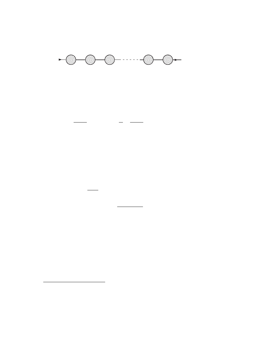
4.2. RENORMALIZATION
71
p
p
Figure 4.5: Iterated self-energy corrections to the propagator
The integral converges nicely, (This is a peculiarity of scalar field theories.
Don’t expect it in general.) so we don’t have to worry about integrating
over fractional dimensions. A straightforward application of (4.19) gives
=
iλ
3
2(4π)
2
Z
1
0
dz
2
Z
1
0
dz
3
1
∆
≡
iλ
3
2(4π)
2
F (p
2
, k
2
, k · p)
(4.32)
The z integrals are difficult;
2
the point is that the triangle diagram con-
tributes a finite function of three scalar quantities, p
2
, q
2
, and p · k.
4.2
Renormalization
Over the course of the last two chapters we have obtained the following.
G(x
1
, x
2
) = h0|T [ϕ(x
1
)ϕ(x
2
)]|0i = iD(x
1
− x
2
)
= i
Z
d
4
k
(2π)
4
e
−ik(x
1
−x
2
)
∆
F
(k)
(4.33)
∆
F
(k) =
1
k
2
− m
2
+ i²
(4.34)
(See equations (3.71), (3.32), (3.44), and (2.108).) It is clear from (3.85)
however, that the last line is only valid for S = 1, i.e. free, non-interacting
fields. Since our purpose is to understand the effects of interactions, we
must be more careful about notation. Let’s use G(x
1
, x
2
) and its Fourier
transform G(p) to represent the exact propagator for a particle to go from x
1
to x
2
, and G
0
(x
1
, x
2
) and G
0
(p) to represent the zeroth-order propagators.
Then G
0
(p) = i∆
F
(p). The exact propagator calculated to all orders of
perturbation theory would have an infinite number of diagrams, or course,
but they could all be parceled up into an infinite sum of diagrams like
Figure 4.5. The lines represent zeroth-order propagators, and each grey
circle represents the sum of all diagrams with one particle in and one particle
2
Actually, Maple and I find them impossible.

72
CHAPTER 4. THE TROUBLE WITH LOOPS
out, which cannot be cut into two pieces by severing a single line.
3
Such
diagrams are said to be one-particle irreducible or 1PI for short. They are
called proper self-energy parts for reasons that will become apparent shortly.
In what is fairly standard notation, we denote them −iΣ(p). The complete
propagator is the sum of diagrams like Fig 4.5 with no self-energy part, one
self-energy part, two parts, etc.
G(p) =G
0
(p) + G
0
(p)
Σ(p)
i
G
0
(p) + G
0
(p)
Σ(p)
i
G
0
(p)
Σ(p)
i
G
0
(p) + · · ·
=G
0
µ
1 +
Σ
i
G
0
+
Σ
i
G
0
Σ
i
G
0
+ · · ·
¶
=G
0
µ
1 −
Σ
i
G
0
¶
−1
=
·
G
−1
0
(p) −
1
i
Σ(p)
¸
−1
=
i
p
2
− m
2
− Σ(p)
(4.35)
There is a deep result independent of perturbation theory that the exact
propagator must have the form
4
G(p) =
i
p
2
− m
2
R
+ i²
+ O(p
2
)
(4.36)
where m
R
is the actual mass of the particle and O(p
2
) is a function of
p
2
with some branch points but no poles. Unless it should turn out that
Σ(p
2
= m
2
) = 0, which I assure you is not the case, the m we have been
carrying around since Chapter 1, is not the actual mass of the particle. What
is worse, both the single loop in Figure 4.2 and the tadpole in Fig 4.3 are
1PI and so are contained in Σ, and they are infinite or at least dependent
on the dimensional parameter ².
We interpret this as follows. The m in (4.35) originally appeared in
the free-particle Lagrangian. As such it represents the mass of a particle
without any interactions. There is no such thing of course, particles are
always interacting, so it’s a kind of meaningless theoretical abstraction. It
is often called the “bare” mass in contrast to m
R
, the renormalized mass.
Therefore
0 =
£
p
2
− m
2
− Σ(p
2
, ²)
¤
p
2
=m
2
R
(4.37)
3
Of course you can always make two pieces by cutting the head off a tadpole. That is
not allowed in this definition.
4
This is called the Lehman spectral representation. See M. E. Peskin and D. V.
Schroeder, An introduction to Quantum Field Theory, Section 7.1

4.2. RENORMALIZATION
73
I have written Σ(p
2
, ²) to emphasize the fact that so long as we keep ²
finite, this is a reasonable mathematical expression. Now expanding Σ in
the vicinity of p
2
= m
2
R
,
Σ(p
2
) ≈ Σ(m
2
R
) + Z
−1
(p
2
− m
2
R
)
(4.38)
where
Z
−1
= −
d
dp
2
Σ(p
2
)
¯
¯
¯
¯
p
2
=m
2
R
(4.39)
Substituting (4.37), (4.38), and (4.39) into (4.35) gives
G(p
2
) =
iZ
p
2
− m
2
R
+ · · ·
(4.40)
This is not quite (4.36) because of the Z factor and for good reason. The
field ϕ(x) that appeared in our Lagrangian is also a free or bare field. It
should also be renormalized by
ϕ
R
(x) = Z
−1/2
ϕ(x)
(4.41)
The factor Z
1/2
is called the wave function renormalization or field renor-
malization. We see from (4.41) that in terms of ϕ
R
the propagator is the
same as that of a free field with mass m
R
, and therefore Z is the same fac-
tor that appeared in the LSZ reduction formula (3.67). In other words, Z
disappears from the LSZ formula if, instead of using the bare field ϕ as we
did in (3.67), we use the “physical” renormalized field. Thus after mass and
wave function renormalization, there are no more bare quantities left in the
propagator.
This is not the whole story however, because we are not given Σ ahead of
time. We can only calculate it in perturbation theory. In order to do pertur-
bation theory right we will need the renormalized mass, the field strength,
and as it turns out, the renormalized coupling constant. It seems we are
caught in another kind of loop. We can’t find Σ until we know m
R
, Z, and
λ
R
, and we can’t find these things until we know Σ. It turns out that we
can make sense of this order by order in perturbation theory. We proceed
as follows. The lowest-order loop contributions come from Figures 4.2 and
4.3. Adding (4.22) and (4.28) we find
−iΣ =
iλ
2
(4π)
2
3
²
+ finite
(4.42)

74
CHAPTER 4. THE TROUBLE WITH LOOPS
By “finite” I mean those terms that remain finite when ² = 0. Let’s say that
in the one-loop approximation
G(p) =
i
p
2
− m
2
R
+ i²
+ finite
=
i
p
2
− m
2
− Σ(p
2
) + i²
+ finite
≈
i
p
2
− m
2
1
+ i²
+ finite
(4.43)
By m
1
I mean the one-loop approximation to the renormalized mass.
m
2
= m
2
1
+
λ
2
(4π)
2
3
²
(4.44)
We can also calculate Z from (4.39)
Z
−1
1
= −
d
dp
2
Σ(p
2
)
¯
¯
¯
¯
p
2
=m
2
1
(4.45)
Notice that the constant is evaluated at p
2
= m
2
1
rather than m
2
R
as in
(4.39). The point is that our approximation is correct to order λ
2
. Using
m
R
rather than m
1
would introduce higher-order corrections.
The triangle diagram, Figure 4.4, modifies the three-particle vertex, but
unlike the mass renormalization, it does so in a way that depends on momen-
tum. We need to choose, somewhat arbitrarily, the kinematic point at which
to make the correction. Simplest is the (unphysical) point p
2
= k
2
= k·p = 0,
in which case ∆ = m
2
, F (0, 0, 0) = 1/m
2
. Consequently the effect of the
one-loop correction is to replace
−iλ → −iλ
1
+
iλ
3
2(4π)
2
m
2
1
(4.46)
or
λ = λ
1
µ
1 +
λ
2
1
2(4π)
2
m
2
1
¶
(4.47)
Again note where λ has been replaced by λ
1
and m by m
1
as appropri-
ate. The implication is that if the one-loop approximation was adequate,
λ
1
and m
1
would be the physical mass and coupling constant, and (4.44)
and (4.47) could be used to remove all reference to m and λ in our cal-
culations. If not, we need to go to two-loop corrections. Let us briefly
consider what this would entail. Figure 4.6 shows a representative sample
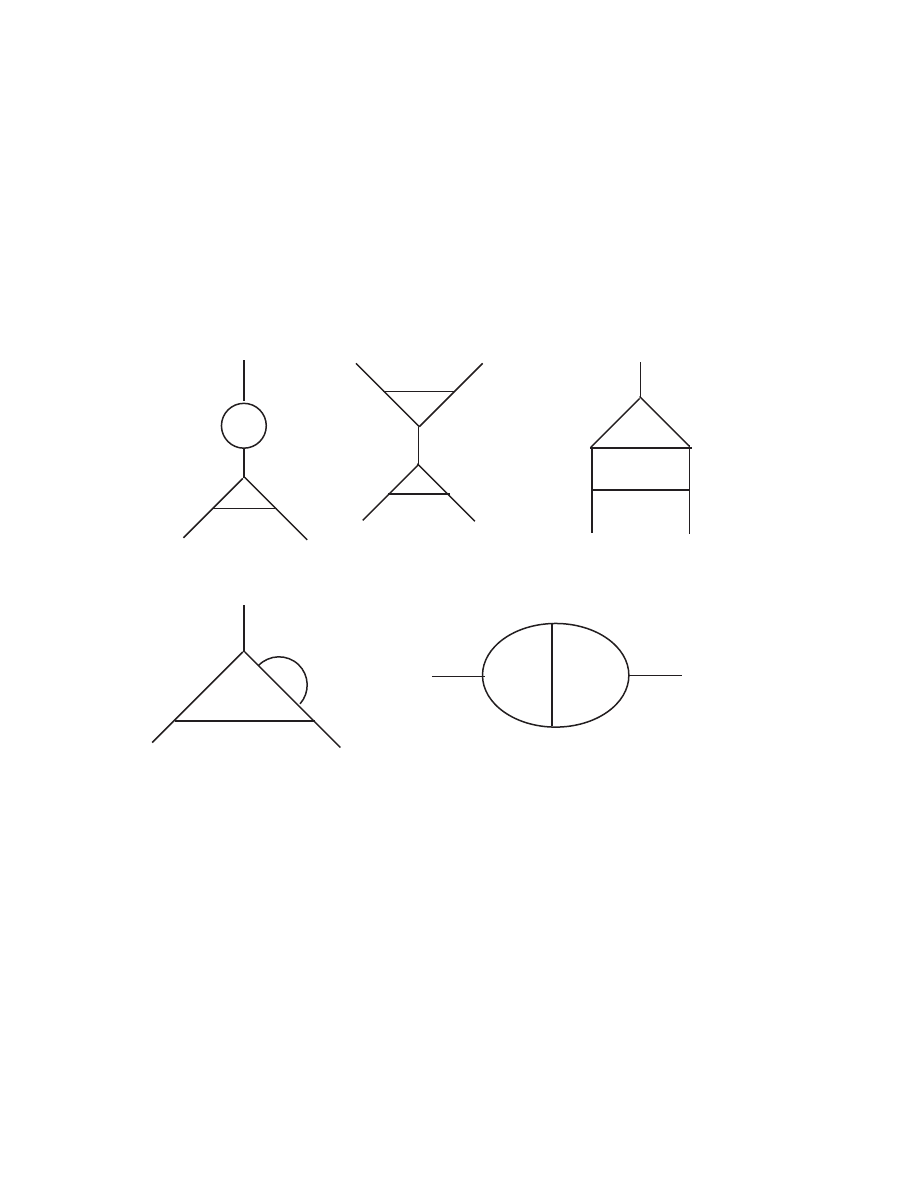
4.2. RENORMALIZATION
75
(a)
(b)
(c)
(d)
(e)
Figure 4.6: Some two-loop diagrams

76
CHAPTER 4. THE TROUBLE WITH LOOPS
of two-loop diagrams. Diagrams (a) and (b) are essentially trivial in that by
cutting a single line they can be separated into two diagrams that we have
already calculated. They are one-particle reducible. The other diagrams
are genuinely new calculations. The λ
3
theory has the peculiarity that most
higher-order diagrams are convergent. Consequently (c) and (e) simply give
finite corrections to everything. Diagram (d) however, illustrates a noto-
rious problem. It contains six propagators and four loop integrals, so the
degree of convergence should be 8-12=-4, i.e. safely convergent. On the
other hand, it contains within it the one-loop correction to the propagator,
which we know diverges. It appears that one gets a finite or infinite answer
depending on the order the two integrals are evaluated. This is an example
of an “overlapping divergence.” These are not so much a problem in QED
because gauge invariance give a tool for dealing with them, but in λ
3
and
especially in the λ
4
theory, they are a severe technical difficulty.
This concludes our study of scalar field theories. Except for the problem
of overlapping divergences, they are child’s play compared with the com-
plexities of QED. They are a good introduction, however, for QED has all
the same features with the additional complication of spin. The λ
4
theory,
moreover, is of more that pedagogical interest. It forms the backbone of
the electroweak theory, the closest thing we have to a theory of everything.
Unfortunately, in this severely truncated course, we will have no time for
that.
4.3
Appendix
Derivation of (4.16)
(
√
π)
d
=
µZ
dx e
−x
2
¶
d
=
Z
d
d
x exp
Ã
−
d
X
i=1
x
2
i
!
=
Z
dΩ
d
Z
∞
0
dx x
d−1
e
−x
2
=
µZ
dΩ
d
¶
·
1
2
Z
∞
0
d(x
2
)(x
2
)
d
2
−1
e − x
2
=
µZ
dΩ
d
¶
·
1
2
Γ(d/2)

4.3. APPENDIX
77
Second derivation
Z
∞
0
d`
`
d−1
(`
2
+ ∆)
2
=
1
2
Z
∞
0
d(`
2
)
(`
2
)
d
2
−1
(`
2
+ ∆)
2
=
1
2
µ
1
∆
¶
2−
d
2
Z
1
0
dx x
1−
d
2
(1 − x)
d
2
−1
where I have substituted x = ∆/(`
2
+ ∆) in the second line. Using the
definition of the beta function
Z
1
0
dx x
α−1
(1 − x)
β−1
= B(α, β) =
Γ(α)Γ(β)
Γ(α + β)
we can easily evaluate the integral over x.
5
Proof of (4.20)
X
²
= exp {ln (X
²
)} = exp {² ln X} = 1 + ² ln X + O(²
2
)
5
These derivations are taken from An Introduction to Quantum Field Theory by M. E.
Peskin and D. V. Schroeder.

78
CHAPTER 4. THE TROUBLE WITH LOOPS

Chapter 5
Cross Sections and Decay
Rates
The last step in the road from Lagrangians to cross sections is this: take
the S-matrix computed in Chapter 7 and convert it to a scattering cross
section or decay rate. There are two easy ways of doing this and one right
way. One easy way is to assume that the initial and final state particles can
be described by plane waves. Plane waves occupy infinite volume, unfortu-
nately, so several key integrals diverge. This problem can be ducked with
some judicious hand waving. The other easy way is to quantize the wave
functions in a box of finite size. This avoids the infinite integrals, but of
course, real experiments aren’t done in a box. It is best to acknowledge that
the beam and target particles should be represented by wave packets, but
this makes for a long tedious derivation. We’ll do it the ssecond easy way
(at least in this edition).
5.1
Classical Scattering
From the point of view of classical mechanics, the cross section of a particle
is just its projected area. If the particle is a sphere of radius R, the cross
section σ
T
= πR
2
. This is usually called the “total” cross section. If the
particle were very small, we might contrive to measure its cross section by
means of a scattering experiment. First we prepare a target with n
t
of
these particles per unit volume, and bombard this target with N
i
incident
point-like particles. We assume that the target is so thin and the target
particles so small that no one of them gets in front of another. We then
count the number N of incident particles that are deflected as a result of a
79

80
CHAPTER 5. CROSS SECTIONS AND DECAY RATES
collision. The fraction of particles that are scattered, N/N
i
must be equal
to the fraction of the target area covered by the projected area of the target
particles, n
t
Lσ
T
, where L is the target thickness. The cross section is then
given by
σ
T
=
N
N
i
n
t
L
The idea works even if σ
T
is arbitrarily small. We just have to make N
i
and
n
t
large enough.
We can also determine the shape with a scattering experiment. Imagine
that the target particles have concentric circles painted on them like an
archery target. If one of the incident particles hits a particular area dσ it
will scatter into a solid angle dΩ. OK – so your’re not as good with a bow
and arrow as Legolas. Just fire a gazillion arrows at random an observe the
distribution of scattering angles. Your favorite theorist should then be able
to infer the shape of the target particle from the distribution. The relevant
equation is
dσ
dΩ
=
1
N
i
n
t
L
dN
dΩ
(5.1)
If you are an experimentalist, you measure dN/dΩ in your lab, compute
dσ/dΩ, and pass it along to the theorist. This computed quantity is called
the “differential cross section.”
The quantities N
i
, n
t
, and L in (5.1) are directly measurable, but for
purposes of comparing with theory, it is more convenient to express them in
terms of flux. If the beam is moving at velocity v toward a stationary target,
then the number of particles in the beam N
i
is equal to the density of the
beam n
i
times the volume. If the beam is a pulse that is turned on for T
seconds, then the volume of the beam is vT A, where A is the cross-sectional
area of the beam (assumed smaller than the target.) Therefore N
i
= n
i
vT A.
The cross section can be written as:
dσ
dΩ
=
1
(n
i
vT A)n
t
L
dN
dΩ
=
1
I
dR
dΩ
,
(5.2)
where the transition rate R is the number of scattering events per unit time
per unit target volume, V = AL.
R = N/V T,
(5.3)
and the flux I is
I = n
i
n
t
v
(5.4)

5.2. QUANTUM SCATTERING
81
5.2
Quantum Scattering
In the quantum mechanics regime, quantities like size and shape don’t have
any direct meaning, since any putative size is bound to be smaller that the
corresponding deBroglie wavelength; but the experiment can still be done
exactly as I have described it, because all the measurements are macro-
scopic and asymptotic. The differential cross section (DCS for short) can’t
be interpreted directly in terms of shape, but it does contain most of the
information we are entitled to have about particles and other subatomic
systems.
The description of scattering in terms of archery targets is appropri-
ate to low-energy potential scattering, but at higher energies new particles
can be created and the total momentum shared among them. It requires
more than a scattering angle to describe the final state. Rather we have
to specify the momenta of each of the particles: p
1
, p
2
, . . . , p
n
. Not all val-
ues of the momenta are allowed of course, because of the conservation of
momentum and energy. We can imagine the momenta as occupying some
complicated-shaped region in a 3n-dimensional space whose coordinates are
the components of the individual momenta. This construct is called “phase
space.”
1
A typical multiparticle scattering experiment measures the transi-
tion probability into some region of phase space. We still use the differential
cross section notation dσ, but now dσ might be an 3n-fold differential, de-
pending on the details of the experiment. I will also use the notation ∆Ω to
indicate some small region of phase space (not just a region of solid angle).
Now let’s put on our theorist’s hats. We know how to calculate the S-
matrix elements. How do we now find the cross sections? You will recall
from the end of Chapter 3 that the first term of the perturbation theory
expansion of the S-matrix describes particles that don’t scatter. Feynman’s
rules decree that all other terms contain the factor (2π)
4
δ
(4)
(P
f
− P
i
), where
P
i
and P
f
are the total momentum four-vectors of the initial and final state
particles. It is customary to define a transition matrix T
f i
as follows:
S
f i
= δ
f i
− i(2π)
4
δ
(4)
(P
f
− P
i
)T
f i
(5.5)
The δ
f i
just represents the particles that don’t scatter. T is the non-trivial
part of the S-matrix with the delta function “peeled off.”
1
Note that phase space in thermodynamics is 6n-dimensional, since it includes space
as well as momentum coordinates.

82
CHAPTER 5. CROSS SECTIONS AND DECAY RATES
There is an alternative notation that is frequently used.
S
f i
= δ
f i
+ i(2π)
4
δ
(4)
(P
f
− P
i
)
Y
i
1
p
2E
i
(2π)
3
Y
f
1
p
2E
f
(2π)
3
M
f i
(5.6)
In the case of the decay of a single particle, the index i = 1, and in the
usual case of two-particle scattering i = 1, 2. The index f runs over all
the final-state particles. Obviously, M
f i
is just T
f i
with the 1/
p
2E(2π)
3
factors peeled off.
If should be clear from (3.24) that the S operator is unitary. The S-
matrix in the current notation is S
f i
= hf |S|ii, where |ii and hf | represent
complete sets of states. As such we expect the S-matrix to be unitary as
well. Very schematically, this means that
X
f
S
∗
f i
S
f k
= δ
ik
(5.7)
I say “very schematically” because it’s not at all clear what it means to sum
over one of these indices. I’ll get back to that.
Since S
f i
is a probability amplitude, we should get the corresponding
probability by squaring it. So for example,
P
f i
= |S
f i
|
2
(5.8)
is the probability that the initial state |ii will scatter into the final state |f i.
Unfortunately this means that we have to square the delta function in (5.5),
and this is bad news, since δ(P
f
− P
i
)δ(P
f
− P
i
) = δ(P
f
− P
i
)δ(0) and δ(0)
is infinite.
I’ll deal with this last problem first. Squaring (5.5) gives
P
f i
= (2π)
4
δ
(4)
(0)(2π)
4
δ
(4)
(P
f
− P
i
)|T
f i
|
2
(5.9)
(I have ignored the non-scattering term.
2
) Here’s the kludge. The factor
(2π)
4
δ
(4)
(0) is interpreted as a volume of space-time, since in the limit P → 0
(2π)
4
δ
(4)
(P ) =
Z
d
4
x e
iP x
→
Z
d
4
x = V T.
(5.10)
2
All textbooks drop the non-scattering term. The reasons are obvious enough. No text
I know of gives any explanation for dropping the interference term between the scattering
and non-scattering terms. This can be partly justified by using wave packets to derive the
scattering formalism, but as a matter of fact, interference effects should be observable at
least in principle in small-angle scattering.

5.2. QUANTUM SCATTERING
83
But the time and volume of what? We can use the derivation of (5.2) as
a model. Let V be a small arbitrary volume inside the interaction region.
Assume that it is small enough to fit inside the beam and target but very
large compared the typical quantum-mechanical dimensions. T is the time
required for a beam particle to pass through V . The analogy to (5.3) is
R
f i
= transition rate per unit volume =
P
f i
V T
=
(2π)
4
V T δ
(4)
(P
f
− P
i
)|T
f i
|
2
V T
=(2π)
4
δ
(4)
(P
f
− P
i
)|T
f i
|
2
(5.11)
This is the first of several instances in which the arbitrary V ’s and T ’s cancel.
Now to the question of counting and normalizing states. This is not
explained clearly in any book I know of, so I hope you will indulge me while
I explain this boring technical detail in excruciating detail. Someone has to
do it.
First of all, Klein-Gordon wave functions have a conserved norm, but it
isn’t
R
dV |ϕ|
2
. In order to have the right behavior under Lorentz transforma-
tions, the norm must transform like the time-like component of a conserved
current. That is, there must be a probability density ρ and a probability
current j such that
∂ρ
∂t
+ ∇ · j = 0
(5.12)
The reason is that the rate of decrease of particles in a given volume is equal
to the total flux of particles out of that volume, that is
−
∂
∂t
Z
V
ρ dV =
Z
S
j · ˆ
n dS =
Z
V
∇ · j dV
The procedure for finding this current should be familiar from nonrelativistic
quantum mechanics. Write the Klein-Gordon equation as
−
∂
2
ϕ
∂t
2
+ ∇
2
ϕ = m
2
ϕ
Multiply this equation by −iϕ
∗
and the complex conjugate equation by −iϕ
and subtract.
∂
∂t
·
i
µ
ϕ
∗
∂ϕ
∂t
− ϕ
∂ϕ
∗
∂t
¶¸
|
{z
}
ρ
+∇ · [−i(ϕ
∗
∇ϕ − ϕ∇ϕ
∗
)]
|
{z
}
j
= 0
(5.13)

84
CHAPTER 5. CROSS SECTIONS AND DECAY RATES
As a consequence the norm is
ρ = i
Z
d
3
x ϕ
∗
(x)
←
→
∂
0
ϕ(x)
(5.14)
By ϕ(x) I mean the wave function, not the quantized field, and
ϕ
∗
←
→
∂
0
ϕ ≡ ϕ
∗
∂
0
ϕ − (∂
0
ϕ
∗
)ϕ.
We have been using the quantized field operator
ˆ
ϕ =
Z
d
3
k
p
(2π)
3
2E
k
h
ˆa
k
e
−ikx
+ ˆ
d
†
k
e
ikx
i
from (2.97). We obtain the classical wave function ϕ from the quantized
field operator ˆ
ϕ as follows
ϕ(x) = h0| ˆ
ϕ(x)|pi =
Z
d
3
k
p
(2π)
3
2E
k
e
−ikx
h0|ˆa
k
ˆa
†
p
|0i
=
e
−ipx
p
(2π)
3
2E
p
(5.15)
This result depends on three normalization conventions that are to some ex-
tent arbitrary. First is the factor 1/
p
(2π)
3
2E in the field operator (2.97).
Second is the commutation relations for the creation and annihilation op-
erators (2.98). Finally, we have agreed to construct single-particle states as
|pi = ˆa
†
p
|0i. Only the equal-time commutation relations (2.102) are non-
negotiable. We will finally arrive at formulas for the cross sections and decay
rates that must be independent of all conventions. This will happen, but no
two books do it the same way!
Our choice of normalization for the field operator has the advantage of
making (2.98) as simple as possible, but it results in a rather odd-looking
norm.
ρ = i(ϕ
∗
←
→
∂
0
ϕ) = 2Eϕ
∗
ϕ = (2π)
−3
Z
V
ρ dV = (2π)
−3
V
(5.16)
Yes that’s right – there are (2π)
−3
particles per unit volume!
Equation (5.11) refers to scattering into a single final state |f i. What
does this mean? Since we already are committed to the imaginary box,
we can impose periodic boundary condition to discretize the momenta. For

5.2. QUANTUM SCATTERING
85
a single particle, quantum theory restricts the number of final states in a
volume V with momenta in element d
3
p to be V d
3
p/(2π)
3
. Our V has
(2π)
−3
V particles, however, so
N
f
=
V d
3
p
(2π)
3
(2π)
−3
V
= d
3
p
(5.17)
In (5.17) N
f
counts the number of discrete quantum states available to a
particle with momentum in the range between p and p + d
3
p, where p in
this case refers to the three-momentum of the particle. In the general case
in which two particles go into N particles with initial and final states given
by
|ii = |k
2
, k
2
i
|f i = |p
1
, p
2
, · · · , p
N
i
(5.18)
the corresponding number is
N
f
=
N
Y
j=1
d
3
p
j
(5.19)
Now turn to the incident flux (5.4). With our norm n
i
= n
t
= (2π)
−3
,
and v is the relative velocity of the colliding particles.
v =
¯
¯
¯
¯
k
1
E
1
−
k
2
E
2
¯
¯
¯
¯ =
1
E
1
E
2
p
(k
1
· k
2
)
2
− (m
1
m
2
)
2
(5.20)
The first expression for v is obviously correct for non-relativistic particles.
The second expression is correct relativistically so long as k
1
and k
2
are
collinear.
The generalization of (5.2) is
dσ =
R
f i
I
N
f
Using (5.11), (5.19) and (5.8) we get
dσ =
1
v
(2π)
10
Z
δ
(4)
(P
f
− P
i
)|T
f i
|
2
N
Y
j=1
d
3
p
j
.
(5.21)
Although dσ is written as if it were a first-order differential, is (5.21) it is
really a 3N -fold differential. For reference we give the same formula using

86
CHAPTER 5. CROSS SECTIONS AND DECAY RATES
the M matrix notation.
dσ =
1
v
1
4E
1
E
2
Z Y
f
d
3
p
f
(2π)
3
2E
f
(2π)
4
δ
(4)
(P
f
− P
i
)|M
f i
|
2
(5.22)
Finally, we use this formalism to compute the probability of the decay
of a single particle. The differential decay rate dΓ of an unstable particle is
defined by
dΓ =
R
f i
n
t
N
f
=(2π)
7
Z
δ
(4)
(P
f
− P
i
)|T
f i
|
2
N
Y
j=1
d
3
p
j
=
1
2E
i
Z Y
f
d
3
p
f
(2π)
3
2E
f
(2π)
4
δ
(4)
(P
i
− P
f
)|M|
2
(5.23)
In this case n
t
is the number of decaying particles per unit volume, which
as usual is equal to (2π)
−3
.
5.3
Phase Space
The outcome of a scattering experiment as described by (5.21) depends,
generally speaking, on three kinds of things. First there are the fundamental
dynamics, which are encoded in the Hamiltonian of the system. Second,
there are the details of the experiment itself, e.g. the number of particles
in the beam and target, the construction of the detectors, etc. There is a
third category of influences that arise because momentum and energy are
conserved and because the experiment must be describable in a relativistic
invariant way. These last considerations are incorporated in the notion of
phase space. Phase space in this context is the set of momentum states
available to the particles after the interaction. Imagine leaving the parking
lot in front of a movie theater after the show is over. If there is only one
narrow road leading out of the lot, then it will take you a long time to
escape. If there are freeways leading out in all directions, the lot will empty
quickly. This is an analogy based on coordinate space. Try to imagine
something like this in momentum space and you will have a feeling for what
phase space means. If there are many momentum states available to the
final-state particles, the scattering cross section will be large or the decay

5.3. PHASE SPACE
87
will happen quickly. I will explain this again in the next paragraph using
a semi-quantitative argument based on the uncertainty principle and finally
present a version of the argument that is correct relativistically.
In classical statistic mechanics the state of motion of a particle is repre-
sented as a point in a six-dimensional manifold called phase space consisting
of three position and three momentum coordinates, i.e. (x, y, z, p
x
, p
y
, p
z
).
Classical mechanics places no restrictions on the density of these points,
since x and p are supposedly measurable with complete precision. Quan-
tum mechanics on the other hand limits the precision by the uncertainty
principle,
∆x
j
∆p
j
≥ 2π¯h.
Phase space can be thought of as being subdivided into elementary cells of
size (2π¯h)
3
. The particle’s coordinates cannot be localized to any smaller
region. The number of states available to one particle will therefore be equal
to the total volume of phase space divided by the size of the elementary
cell. Assuming that the particle is contained in a volume V , the number of
available states is
N =
1
(2π¯h)
3
Z
d
3
x d
3
p =
V
(2π¯h)
3
Z
d
3
p.
The limits of integration come about from the conservation of mass and
energy. Since p
µ
p
µ
= m
2
, the momentum integration is bounded by a sphere
of radius |p|
2
= E
2
− m
2
, so that N depends on m and E. The factor
V /(2π¯h)
2
is part of the normalization discussed in the previous section. I
am concerned here with the integral over d
3
p.
Now suppose there are N such particles in the final state of a scattering
experiment.
N
N
=
Z
N −1
Y
j=1
d
3
p
j
(5.24)
There are only N − 1 integrals in (5.24), because the N p
j
’s are not all
independent,
N
X
j=1
p
j
≡ P
f
= P
i
.
We can incorporate this constraint in a more flexible way by introducing a
δ-function.
Z
d
3
p
N
δ
(3)
Ã
p
N
+
N −1
X
k=1
p
k
− P
i
!
= 1

88
CHAPTER 5. CROSS SECTIONS AND DECAY RATES
N
N
=
Z
N −1
Y
j=1
d
3
p
j
=
Z
N
Y
j=1
d
3
p
j
δ
(3)
Ã
N
X
k=1
p
k
− P
i
!
Energy is also conserved, and this constraint can be included with a similar
trick.
Z
dE
i
δ(E
f
− E
i
) = 1
N
N
=
Z
dE
i
N
Y
j=1
d
3
p
j
δ
(3)
Ã
N
X
k=1
p
k
− P
i
!
δ
Ã
N
X
k=1
E
k
− E
i
!
dN
N
dE
i
=
Z
N
Y
j=1
d
3
p
j
δ
(4)
(P
f
− P
i
)
(5.25)
These are just the kinematic factors appearing in (5.21). It appears from
this heuristic argument, that the reaction rate is proportional to the density
of states dN
N
/dE
i
.
3
This is not the whole story, because (5.25) as it stands
is not Lorentz invariant, but according to the Feynman rules from Section
3.5, the square of the scattering amplitude, |hf |T |ii|
2
in (5.21), contains a
factor 1/2E
i
(2π)
3
for each particle in the final state. This is good, since
Z
d
4
p δ(p
2
− m
2
) =
Z
d
3
p
2E
is clearly a Lorentz scalar. The point is that the factors
N
Y
j=1
Z
d
3
p
j
(2π)
4
δ
(4)
(P
i
− P
f
)
from (5.21) together with the factors 1/2E
i
from |hf |T |ii|
2
can be combined
into a Lorentz-invariant quantity
P =
Z
N
Y
j=1
d
3
p
j
2E
j
δ
(4)
(P
f
− P
i
)
=
Z
N
Y
j=1
d
4
p
j
δ(p
2
j
− m
2
) δ
(4)
(P
f
− P
i
)
(5.26)
3
You will recall from elementary quantum mechanics that the transition probability
rate for a system to make a transition from an energy E
l
to E
k
is given by “Fermi’s golden
rule,”
w
lk
=
2π
¯h
g(E
k
)|H
kl
|
2
where g(E
k
) is the density of states whose energy is close to E
k
. See R. L. Liboff, Intro-
ductory Quantum Mechanics.

5.4. TWO-PARTICLE SCATTERING
89
The quantity P is called the Lorentz-invariant phase space. In general we
are more interested in integrating some of the momenta in (5.26) over some
portion of their allowed kinematic range, in which case
dP =
Z
p∈∆
N
Y
j=1
d
4
p
j
δ(p
2
j
− m
2
)δ
(4)
(P
f
− P
i
).
(5.27)
You might say that (5.26) and (5.27) lie on the interface between theory and
experiment. For example, if you were using (5.21) to predict the results of an
experiment, the limits on the integrals would be set to represent the details
of the experimental apparatus. If the apparatus did not detect particle j (it
might be a neutral particle), then the corresponding momentum p
j
would
be integrated out. If the momentum of the k’th particle was measured, then
the corresponding integral would not be done, and P would be left as a
function of p
k
.
For many-particle reactions, P will have a complicated dependence on
the momentum variables.
4
It is often the case that the data from an ex-
periment are determined mostly by P regardless of the dynamics. Such
an experiment is a failure almost by definition. The general purpose of an
experiment is always to find some deviation from phase space.
5.4
Two-Particle Scattering
To make this more concrete, let’s calculate the cross section for the elastic
scattering of two particles k
1
+k
2
→ p
1
+p
2
from the example in the previous
chapter. Comparing (3.91) (with Z = 1) with (5.5) gives
T
f i
=
λ
(2π)
6
p
2E
k
1
2E
k
2
2E
p
1
2E
p
2
(5.28)
Then (5.21) gives
dσ =
λ
2
4(2π)
2
vE
k
1
E
k
2
Z
d
3
p
1
2E
p
1
d
3
p
2
2E
p
2
δ
(4)
(P
f
− P
i
)
=
λ
2
4(2π)
2
vE
k
1
E
k
2
Z
dP
(5.29)
The transition matrix T
f i
is especially simple in this example. This is why
there is nothing inside the integral except dP. In general there will be some
complicated function that we may or may not want to integrate.
4
There are entire books written on the subject, e.g. Kinematics and Multiparticle
Systems, M. Nikolic, Gordon and Breach (1968)

90
CHAPTER 5. CROSS SECTIONS AND DECAY RATES
I will complete the calculation in the center of mass system assuming
equal-mass particles. In this case |k
1
| = |k
2
| = |p
1
| = |p
2
|, k
1
= −k
2
,
p
1
= −p
2
, E
p
2
= E
p
1
≡ E
1
, and E
k
1
+ E
k
2
≡ E
i
. For the remainder of this
section only I will use the notation |p
1
| = p
1
. Integrating out d
3
p
2
gives
P =
Z
1
4E
2
1
p
2
1
dp
1
δ(2E
p
1
− E
i
)dΩ
1
It’s convenient to change the variable of integration from p
1
to E
1
.
p
1
dp
1
= E
1
dE
1
δ(2E
1
− E
i
) =
1
2
δ(E
1
− E
i
/2)
P =
Z
p
1
8E
1
dE
1
δ(E
1
− E
i
/2)dΩ
1
There is still one δ-function, which will enforce energy conservation and
hence fix the value of p
1
.
P =
Z
p
1
8E
1
dΩ
1
=
πp
1
4E
1
.
(5.30)
Notice that symmetry together with the conservation of momentum and
energy largely predetermine the outcome of such a scattering experiment.
If the particles are spinless there can be no dependence on the azimuthal
angle. Only the scattering angle θ
1
is unconstrained, and the only way
the underlying dynamics could manifest itself is by affecting the differential
cross section as a function of scattering angle. Our example is trivial in the
sense that there is no θ dependence, but let’s go ahead and calculate the
differential cross section anyhow. For this purpose it is best to leave (5.30)
in the form of a differential
dP =
p
1
8E
1
dΩ
1
(5.31)
We also need v from (5.20), which in this simple case gives
v =
2p
1
E
1
(5.32)
Equation (5.29) becomes
dσ =
λ
2
4(2π)
2
E
2
1
E
1
2p
1
p
1
8E
1
dΩ
1
dσ
dΩ
1
=
λ
2
(16πE
1
)
2
(5.33)
As anticipated, the scattering is isotropic. There is no θ
1
dependence.

5.5. THE GENERAL CASE
91
5.5
The General Case
Here is a cookbook procedure for calculating scattering cross sections and
decay rates for the general case in which there are N particles in the final
state.
• Use Feynman’s rules from Section 3.5 to calculate the S matrix.
• Find the transition matrix T
f i
from (5.5).
• Find the relative velocity v from (5.20).
• The differential cross sections and decay rates are calculated from
(5.21) and (5.23) integrated over the appropriate regions of phase
space.
dσ =
(2π)
10
v
Z
p∈∆Ω
N
Y
j=1
d
3
p
j
δ
(4)
(P
f
− P
i
)|T
f i
|
2
(5.34)
dΓ = (2π)
7
Z
p∈∆Ω
N
Y
j=1
d
3
p
j
δ
(4)
(P
f
− P
i
)|T
f i
|
2
(5.35)
When there are only two particles in the final state, one integrates
over all the momentum components that are constrained by the delta
function and leaves the remaining two angles in the form of a differ-
ential. When there are more than two particles in the final state, the
decision regarding which variables to integrate and which to leave in
the differential depends on the experiment that the theory is describ-
ing. That is the meaning of the notation p ∈ ∆Ω that specifies the
limits of the integrals
Because of our normalization conventions, |T
f i
|
2
will contain one factor of
1/(2π)
3
2E for each external particle in the reaction. The factors of 2π as well
as the energies of the initial-state particles are constants that are gathered
together outside the integrals. The energies of the final-state particles are
functions of the variables of integration. It is best to think of them as part of
the phase space defined by (5.26). Needless to say, these rules are tailored
to the Feynman’s rules from Section 3.5. If you combine formulas from
different books, you are likely to get the wrong answer.
The rules so far only hold for spinless particles. The Dirac wave functions
used for spin-
1
2
scattering are normalized differently. I’ll return to that point
at the end of Chapter 6.

92
CHAPTER 5. CROSS SECTIONS AND DECAY RATES

Chapter 6
The Dirac Equation
There is a story to the effect that Neils Bohr once asked Dirac what he was
working on. Dirac, who was famous for not saying much, replied, “I’m try-
ing to take the square root of the Klein-Gordon equation.” The background
to the story is this: the Klein-Gordon equation is invariant under Lorentz
transformations, but it was known to have a strange pathology, it has nega-
tive energy solutions. This is inevitable with a second-order equation. The
Schrodinger equation, on the other hand, is hopeless so far as relativity is
concerned, but because it has only a first derivative with respect to time,
it has only positive-energy solutions. (I’m talking about free-particle equa-
tions here. Bound state problems usually have negative total energy.) Dirac
thought that he could combine the two equations in a way that would pre-
serve the best features of each. The result is called the Dirac equation.
Ironically, it has negative-energy solutions anyway, but it does provide a
formalism for treating spin 1/2 particles in a way that is consistent with
relativity.
6.1
The Equation
Let’s follow in the footsteps of our taciturn master and see what we can
come up with. Start with the Schrodinger equation.
i
∂ψ
∂t
= Hψ
Can we come up with a Hamiltonian that (1) is first order in space deriva-
tives, (2) is Hermitian, and (3) leads to a covariant equation of motion? The
93

94
CHAPTER 6. THE DIRAC EQUATION
answer is yes if ψ is a matrix. Try
i
∂ψ
∂t
= Hψ = (α · p + βm)ψ
(6.1)
here α and β are Hermitian matrices and p = −i∇. We will also use the
replacement E = i∂/∂t. If E is the total energy of special relativity, it must
satisfy E
2
= p
2
+ m
2
. Combine this with equation (6.1)
E
2
ψ =
µ
i
∂
∂t
¶
2
ψ = (α · p + βm)
µ
i
∂ψ
∂t
¶
= (α · p + βm)
2
ψ
We would like this to equal (p
2
+ m
2
)ψ. This will be possible if the matrices
have some special properties.
(α
i
p
i
+ βm)
2
= β
2
m
2
+ (α
i
)
2
(p
i
)
2
+ {α
i
, β} mp
i
+
1
2
{α
i
, α
j
}
i6=j
p
i
p
j
(6.2)
I have used the convention that repeated indices are summed. The curly
brackets are endemic to Diracology. They represent the anticommutator.
{A, B} ≡ AB + BA
We would like (6.2) to boil down to p
i
p
i
+ m
2
. This will be possible if these
matrices obey the following constraints:
β
2
= (α
i
)
2
= 1 for each i
(6.3)
{α
i
, β} = {α
i
, α
j
}
i6=j
= 0
(6.4)
We are trying to construct a theory of spin 1/2 particles, and we know
that in non-relativistic QM Pauli spinors have two components. We expect
therefore that α and β will be 2 × 2 matrices. Alas, it is not to be. They
must be at least 4 × 4. Here is the argument:
1. βα
i
+α
i
β = 0 so βα
i
β = −α
i
β
2
= −α
i
. Take the trace of this equation.
T r[βα
i
β] = T r[α
i
β
2
] = T r[α
i
] = −T r[α
i
]. So α
i
is traceless. In the
same way we could prove that T r[β] = 0.
2. We want α and β to be Hermitian. This together with (6.3) is sufficient
to prove that their eigenvalues are ±1
3. Arguments 1. and 2. lead us to conclude that the matrices must have
even dimension.

6.1. THE EQUATION
95
4. There are only three independent traceless Hermitian 2 × 2 matrices,
and you know what they are: the Pauli spin matrices.
σ
1
=
µ
0 1
1 0
¶
σ
2
=
µ
0 −i
i
0
¶
σ
1
=
µ
1
0
0 −1
¶
(6.5)
Unfortunately, we need four such matrices, so 2×2 won’t do. We must
have 4 × 4. The traditional choice is
β =
µ
I
0
0 −I
¶
α
i
=
µ
0 σ
i
σ
i
0
¶
(6.6)
All this has a nasty, non-relativistic look about it. We therefore abandon
Dirac’s original notation for the following:
1
γ
0
= β
γ
i
= βα
i
=
µ
0
σ
i
−σ
i
0
¶
(6.7)
Now (6.4) becomes
{γ
µ
, γ
ν
} = 2g
µν
(6.8)
and (6.1) is
(iγ
µ
∂
µ
− m)ψ = 0
(6.9)
This is Dirac’s equation. Of course ψ is a four-component column matrix,
the so-called Dirac spinor. g
µν
is the usual metric tensor. There is one other
convenient bit of notation.
γ
µ
B
µ
= γ
µ
B
µ
≡6 B
(6.10)
Dirac’s equation finally is (i 6 ∂ − m)ψ = 0. It looks simple. It’s not. It is
however, covariant. This is far from obvious, but I will not prove it at this
time.
Wave functions are supposed to have something to do with probability.
This is true of ψ as well, but to see the connection, we need to derive
the formula for a conserved current. Starting with (6.1) and taking the
Hermitian conjugate, we have
−i
∂ψ
†
∂t
= i
∂ψ
†
∂x
i
α
i
+ ψ
†
βm
(6.11)
1
Some authors use different conventions. This is consistent with Zee, Gross, and many
other texts.

96
CHAPTER 6. THE DIRAC EQUATION
Multiply on the right by β
2
= 1 and define
ψ ≡ ψ
†
β = ψ
†
γ
0
(6.12)
This object ψ is called the Dirac conjugate. It often appears in bilinear
expressions in place of the usual Hermitian conjugate. Anyhow, the resulting
equation is
−i
∂ψ
∂t
γ
0
= −i
∂ψ
∂x
i
γ
i
+ ψm
or
ψ(i
←
6 ∂ +m) = 0
(6.13)
The arrow indicates that the derivative acts to the left. To find the current,
multiply (6.9) on the left by ψ and (6.13) on the right by ψ and add the
two. The result is
∂
µ
ψγ
µ
ψ + ψγ
µ
∂
µ
ψ = 0 = ∂
µ
(ψγ
µ
ψ)
(6.14)
So the conserved current is
j
µ
= ψγ
µ
ψ
(6.15)
The current density j
0
= ψ
†
ψ is positive and has the same form |ψ|
2
as the
probability density in non-relativistic QM.
6.2
Plane Wave Solutions
We know that electrons have two spin components. Why then are there four
components to the Dirac spinor? The answer is that despite Dirac’s best
intentions, there are still negative energy solutions. This in turn is related
to the existence of antiparticles. We will get to the particle interpretation
later. For the time being we will just reconcile ourselves to negative energies.
We start with
ψ
±
= e
∓ipx
µ
χ
η
¶
(6.16)
As a convention, the symbol E = p
0
will always refer to a positive number.
χ and η are two-component spinors. They are not independent; the Dirac
equation imposes a relationship between the two. Our job is to find it. Start
with the upper sign (positive energy) solution. Substitute (6.16) into (6.1).
µ
E − m −σ · p
−σ · p E + m
¶ µ
χ
η
¶
= 0

6.2. PLANE WAVE SOLUTIONS
97
This will only have a solution if the determinant is equal to zero, i.e. E
2
−
m
2
− (σ · p)
2
= 0. Remember that
σ
2
i
= I
{σ
i
, σ
j
}
i6=j
= 0
(6.17)
so that
(σ · p)
2
= p
2
,
(6.18)
which is a useful identity to have at your disposal. We conclude that E
2
=
p
2
+ m
2
, which we knew anyhow. Unfortunately, this means that E =
±
p
p
2
+ m
2
, so we are stuck with negative energy solutions. At any rate
η =
µ
σ · p
E + m
¶
χ
We can make χ into a Pauli spinor that satisfies χ
†
χ = 1.
χ
(1)
=
µ
1
0
¶
χ
(2)
=
µ
0
1
¶
(6.19)
The complete positive energy solution to the Dirac equation is written
ψ
+
(x, s) = u(p, s)e
−ipx
(6.20)
where
u(p, s) = C
χ
(s)
·p
E+m
χ
(s)
s = 1, 2
(6.21)
Notice that in the non-relativistic limit, the third and fourth components
become negligible.
The normalization constant C has to be chosen according to some con-
vention. We will use u(p, s)u(p, s) = 1. In order to appreciate this, it is
necessary to use one of these group theory results that I have not yet proved.
It is a fact that combinations like ψψ and uu are Lorentz scalars, so that
if we choose the normalization in the rest frame of the particle, it will have
the same value in all other frames. A quick calculation shows that
u(p, s)u(p, s) = C
2
2m
E + m
,
so our normalized spinor is
u(p, s) =
r
E + m
2m
χ
(s)
·p
E+m
χ
(s)
s = 1, 2
(6.22)

98
CHAPTER 6. THE DIRAC EQUATION
so that in the rest frame
u(0, 1) =
1
0
0
0
u(0, 2) =
0
1
0
0
(6.23)
Now back to the negative energy solutions, which I will provisionally call
u(p, 3) and u(p, 4). Repeating the above arguments with the lower sign in
(6.16) brings us to
χ = −
µ
σ · p
E + m
¶
η
and
u(p, s) =
r
E + m
2m
−
·p
E+m
χ
(s−2)
χ
(s−2)
s = 3, 4
(6.24)
It is easy to see that in the rest frame (and so everywhere else) (6.24) is
normalized so that u(p, s)u(p, s) = −1. The minus sign is forced on us. The
complete negative-energy solution is
ψ
−
(x, s) = u(p, s)e
ipx
s = 3, 4
(6.25)
6.3
Charge Conjugation and Antiparticles
The appearance of negative-energy states was both an embarrassment and a
disappointment; a disappointment because this wasn’t supposed to happen
with a linear wave equation and an embarrassment because of its physical
implications. Let us consider an atomic electron. An excited electron will
normally lose energy by emitting photons until it drops down to the lowest-
energy or ground state. In the original version of Dirac theory there is no
lowest-energy state since there exists an continuum of negative-energy states
from −mc
2
to −∞. The electron would fall into a bottomless pit emitting
an infinite amount of energy in the process! To sidestep this difficulty, Dirac
proposed that under normal circumstances, all negative-energy states are
completely filled. This agglomeration of filled states is called the Dirac sea.
Like all of our theories I suppose, it’s a half truth. Unfortunately, the other
half is very confusing. For one thing, it depends on the Pauli exclusion
principle. The states are full because no two Fermions can occupy a single
state. This is not true for integer spin particles, and the Klein-Gordon

6.3. CHARGE CONJUGATION AND ANTIPARTICLES
99
equation also has negative energy states. Obviously the Dirac sea can’t be
the whole answer, but it contains a surprising amount of physical insight.
2
Suppose one of the negative-energy electrons were to absorb a photon of
energy > 2mc
2
and become an E > 0 state. As a result a “hole” is created
in the Dirac sea. The observable energy of the Dirac sea is now the energy
of the vacuum minus the negative energy of the vacated state, hence a pos-
itive quantity. In this way we expect that the absence of a negative-energy
electron appears as the presence of a positive-energy particle. The same
argument works with charge. Let Q
0
represent the charge of the vacuum
and e the negative charge of an electron in the sea, then the total charge of
the Dirac sea is
Q = Q
0
− e = Q
0
− (−|e|) = Q
0
+ |e|
(6.26)
The observable charge is then Q
obs
= Q − Q
0
= |e|. This is interpreted as a
particle with positive energy and charge. This process actually happens. In
the laboratory it looks like γ → e
−
+ e
+
. (It can’t happen in empty space
because of energy and momentum conservation. It does happen whenever
high energy photons pass through matter.) When Dirac first proposed this
in 1930, however, no such particle was known. For this reason it was as-
sumed that the theory couldn’t be right. The positron was discovered soon
thereafter.
According to this theory, the total energy of the vacuum as well as the
total charge is negative infinity. We have to take it on faith that these
infinities are not observable. What is observable are the deviations from
infinity corresponding to the energy and charge of a single electron! This is
an unsatisfactory aspect of the theory of course, but it will continue to devil
us long after we have abandoned the Dirac sea.
The argument made above regarding charge and energy also works for
momentum and spin. The absence of momentum p in the Dirac sea appears
as the presence of momentum −p. Similarly the absence of a spin-up E < 0
electron is to be interpreted as the presence of a spin-down E > 0 positron.
This is all well and good, but we must face the fact that the Dirac
sea is really just a metaphor. We need to describe antiparticles in a way
that does not invoke negative energies. I once heard Edward Teller explain
antiparticles like this: “Take a particle in one hand and an antiparticle in
the other. Put them together, and what you have is – nothing”! Put less
cryptically, all the additive quantum numbers sum to zero. What are the
2
The best discussion of this entire subject is still the classic, Advanced Quantum Me-
chanics, by J. J. Sakurai, Addison-Wesley 1967, Sections 3.9-3.10

100
CHAPTER 6. THE DIRAC EQUATION
additive quantum numbers? Well, charge, baryon number, three kinds of
lepton number, and strangeness for starters. Electrons have zero baryon
number and strangeness anyhow. I will come to the issue of lepton number
presently. Let’s concentrate on the matter of charge. We can define a
transformation called “charge conjugation.” It has two effects. First, it
replaces all particles with their antiparticles, and second, it changes the
wave function in such a way that it correctly describes the new situation.
It’s easy to modify the Dirac equation to include the electromagnetic
potential. The procedure is called “minimal substitution.” The rule is
everywhere you see the derivative ∂
µ
simply replace it with ∂
µ
→ D
µ
=
∂
µ
+ iqA
µ
where q is the charge of the particle. This rule is based on the
idea of gauge invariance, which we will discuss in the next chapter. For the
time being – just believe it. With this replacement the Dirac equation for
an electron with charge −e (e > 0) becomes
(i 6 ∂ + e 6 A − m)ψ = 0
(6.27)
Charge conjugation must change the charge of the electron so that Teller’s
dictum comes true. The transformed equation is
(i 6 ∂ − e 6 A − m)ψ
c
= 0.
(6.28)
Here ψ
c
is the new “charge conjugated” wave function. Take the complex
conjugate of (6.28) and multiply by C
0
, a 4 × 4 matrix that operates on the
space of the γ’s.
C
0
(iγ
µ∗
∂
µ
+ eγ
µ∗
A
µ
+ m)ψ
∗
c
=
£
(C
0
γ
µ∗
C
−1
0
)(i∂
µ
+ eA
µ
) + m
¤
C
0
ψ
∗
c
= 0
(6.29)
At this point we don’t know what C
0
is. The challenge is to get (6.28)
looking like (6.27). For this we will need C
0
γ
µ∗
C
−1
0
= −γ
µ
and C
0
ψ
∗
c
= ψ.
It doesn’t take much trial and error to realize that all the γ’s are pure real
except γ
2
. Try C
0
= iγ
2
. (The i is necessary to make C
0
Hermitian.)
3
You
can check that C
2
0
= I and C
0
γ
µ∗
C
−1
0
= −γ
µ
as promised. The bottom line
is
ψ
c
= C
0
ψ
∗
= iγ
2
ψ
∗
(6.30)
Let us see what this operation does to our prefab spinors. The following
identities are useful.
σ · p =
µ
p
z
p
−
p
+
−p
z
¶
(6.31)
3
There are several different representations of the gamma matrices that are useful in
other contexts. Equation (6.30) is valid only in the the standard or Dirac-Pauli represen-
tation we are using.

6.3. CHARGE CONJUGATION AND ANTIPARTICLES
101
C
0
=
0 0 0 −1
0 0 1
0
0 1 0
0
−1 0 0
0
(6.32)
ψ
+
(x, 1) = u(p, 1)e
−ipx
=
r
E + m
2m
1
0
p
z
/(E + m)
p
+
/(E + m)
e
−ipx
(6.33)
ψ
+
(x, 2) = u(p, 2)e
−ipx
=
r
E + m
2m
0
1
p
−
/(E + m)
−p
z
/(E + m)
e
−ipx
(6.34)
ψ
−
(x, 3) = u(p, 3)e
ipx
=
r
E + m
2m
−p
z
/(+m)
−p
+
/(E + m)
1
0
e
+ipx
(6.35)
ψ
−
(x, 4) = u(p, 4)e
ipx
=
r
E + m
2m
−p
−
/(E + m)
p
z
/(E + m)
0
1
e
+ipx
(6.36)
Let’s find the charge-conjugated version of ψ
+
(x, 1). Using (6.30), (6.32),
and (6.33) gives
ψ
+
c
(x, 1) =
0 0 0 −1
0 0 1
0
0 1 0
0
−1 0 0
0
r
E + m
2m
1
0
p
z
/(E + m)
p
+
/(E + m)
∗
e
+ipx
=
r
E + m
2m
−p
−
/(E + m)
p
z
/(E + m)
0
−1
e
+ipx
= −u(−p, 4)e
ipx
(6.37)
In the same way one can prove that
ψ
+
c
(x, 2) = u(−p, 3)e
ipx
(6.38)
Thus the charge-conjugate wave function obtained from the positive-energy
plane-wave solution is the wave function for a negative-energy plane wave

102
CHAPTER 6. THE DIRAC EQUATION
with the same |E| and opposite momentum. The spin direction is also
reversed since the spin-up spinor with s = 1 is changed into the spin-down
spinor with s = 4. According to Dirac’s hypothesis, the observable behavior
of the charge-conjugate wave function should be a positron with E > 0 and
the same momentum and spin. This is consequence of the absence of an
electron with negative charge and energy and reversed momentum and spin.
If you buy into this bizarre notion of the Dirac sea, the rest is logically
consistent, but expectation values of the charge-conjugated wave functions
do not give the results you would like in terms of antiparticles. Try for
example, to calculate the expectation value of the charge of a positron. The
electromagnetic current should be proportional to the zeroth component of
the probability current (6.15).
Q = e
Z
j
0
d
3
x = e
Z
ψ
†
ψd
3
x
(6.39)
The charge-conjugated wave functions give the same value for Q, since
Q
c
= e
Z
ψ
†
c
ψ
c
d
3
x = e
Z
(C
0
ψ
∗
)
†
(C
0
ψ
∗
)d
3
x = e
Z
(ψ
†
ψ)
∗
d
3
x = Q (6.40)
where I have used the fact that C
0
is Hermitian, C
2
0
= I, and currents
are real functions. It’s trivial to show that the expectation values of the
momentum and spin do change sign. The reason is that ψ
c
is not the positron
wave function, it’s the wave function that is interpreted as the positron
wave function. Under the skin, it’s still the wave function of a fictitious
negative energy particle.
4
In order to get sensible expectation values we
need to introduce second quantization with creation operators that create
real positrons. In order to do that, it is customary to define spinors for real
positrons as follows.
v(p, 1) ≡ −u(−p, 4)
v(p, 2) ≡ +u(−p, 3)
(6.41)
With this definition
u
c
(p, s) = C
0
u(p, s)
∗
= v(p, s)
s = 1, 2
v
c
(p, s) = C
0
v(p, s)
∗
= u(p, s)
s = 1, 2
(6.42)
u(p, 3) and u(p, 4) are properly called negative-energy spinors, while v(p, 1)
and v(p, 2) are positron spinors.
4
Again – thanks to Sakurai for finally making me understand this point.

6.4. QUANTIZING THE FIELD
103
Here is a summary of the important equations involving u and v:
ψ
+
(x) = u(p, s)e
−ipx
(6.43)
ψ
−
(x) = v(p, s)e
+ipx
(6.44)
u(p, s)u(p, s
0
) = −v(p, s)v(p, s
0
) = δ
ss
0
(6.45)
u
†
(p, s)u(p, s
0
) = v
†
(p, s)v(p, s
0
) =
E
m
δ
ss
0
(6.46)
u(p, s)v(p, s
0
) = v(p, s)u(p, s
0
) = 0
(6.47)
u
†
(−p, s)v(p, s
0
) = v
†
(p, s)u(−p, s
0
) = 0
(6.48)
X
s
u(p, s)u(p, s) =
µ
6 p + m
2m
¶
(6.49)
X
s
v(p, s)v(p, s) =
µ
6 p − m
2m
¶
(6.50)
These equations will all be useful later on. You can verify them by substi-
tuting the representations (6.22), (6.24), and (6.7).
6.4
Quantizing the Field
We repeat the procedure from Chapter 5 used to quantize the Kline-Gordon
field. First we’ll need a Lagrangian, which can be taken as
L = ψ(x)(i 6 ∂ − m)ψ(x)
(6.51)
The conjugate momentum is
π =
∂L
∂ ˙
ψ
= iψ
†
(6.52)
and the Hamiltonian is
H =
Z
d
3
x (π ˙
ψ − L) =
Z
d
3
x ψiγ
0
∂
0
ψ
(6.53)
Next we will need the plane wave solutions of the Dirac equation. These are
u(p, s)e
−ipx
and v(p, s)e
ipx
. We then expand ψ(x) and π(x) in a Fourier
series in which creation and annihilation operators appear as Fourier coeffi-
cients. This should look like (2.93) with the following differences:

104
CHAPTER 6. THE DIRAC EQUATION
1. ψ is a four-component spinor rather than a scalar like ϕ.
2. u(p, x) and v(p, s) depend on spin, so in addition to integrating over all
momentum components, we must also sum over the spin components.
3. We need two kinds of creation and annihilation operators, one set for
electrons and one for positrons. In the usual notation
b(p, s)
Annihilates a positive energy electron
b
†
(p, s) Creates a positive energy electron
d(p, s)
Annihilates a positive energy positron
d
†
(
p, s)
Creates a positive energy positron
(6.54)
The analogs to (2.93) are
ψ(x) =
Z r
m
E
d
3
p
p
(2π)
3
X
s
[b(p, s)u(p, s)e
−ipx
+ d
†
(p, s)v(p, s)e
ipx
]
ψ(x) =
Z r
m
E
d
3
p
p
(2π)
3
X
s
[b
†
(p, s)u(p, s)e
ipx
+ d(p, s)v(p, s)e
−ipx
]
(6.55)
In analogy with (2.102) we would expect the equal-time commutation rela-
tions to be
[ψ
α
(x, t), ψ
†
β
(y, t)] = δ
αβ
δ
3
(x − y)
[ψ
α
(x, t), ψ
β
(y, t)] = [ψ
†
α
(x, t), ψ
†
β
(y, t)] = 0.
Unfortunately, this leads to some wildly unphysical consequences. The ori-
gin of the problem is that electrons are fermions, i.e. particles with half-odd
integer spin. Such particles obey the Fermi exclusion principle, no two par-
ticles can occupy the same quantum state. Mathematically, this means that
creation and annihilation operators anticommute, and so as a consequence,
must the fields themselves. We must have
n
ψ
α
(x, t), ψ
†
β
(y, t)
o
= δ
αβ
δ
3
(x − y)
{ψ
α
(x, t), ψ
β
(y, t)} =
n
ψ
†
α
(x, t), ψ
†
β
(y, t)
o
= 0.
(6.56)
Pay careful attention to the notation. ψψ
†
is a 4 × 4 matrix,
whereas ψ
†
ψ is a 1 × 1 matrix, so [ψ, ψ
†
] doesn’t make any sense.
The commutators in (6.56) refer to the α-th component of one
ψ matrix with the β-th component of another. Put it another
way, each commutator is a 4 × 4 matrix with rows and columns
indexed by α and β. Be alert to this ambiguity in other contexts.

6.4. QUANTIZING THE FIELD
105
You should verify that (6.55) is consistent with (6.56) assuming the following
anticommutation relations
n
b(p, s), b
†
(p
0
, s
0
)
o
= δ
ss
0
δ
3
(p − p
0
)
n
d(p, s), d
†
(p
0
s
0
)
o
= δ
ss
0
δ
3
(p − p
0
)
(6.57)
All other combinations of b and d anticommute. The factor of
p
m/E in
(6.55) was chosen so that (6.56) would come out right.
There are at least three places where we have to make a some-
what arbitrary choice of normalization. One is the normalization
of u and v, equations (6.22) and (6.24). The second is the above-
mentioned factor in the Fourier expansion of ψ. The third is the
normalization of the creation and annihilation operators, (6.57).
Only (6.56) is non-negotiable. It is only a slight exaggeration to
say that no two books do it the same way. At least Zee, Michio
Kaku (Quantum Field Theory, A Modern Introduction), and I
are consistent.
It’s easy to generalize charge conjugation (6.30) for the quantized fields.
Define the charge conjugation operator ˆ
C by
ˆ
ψ
c
≡ ˆ
C ˆ
ψ ˆ
C
−1
= C
0
ˆ
ψ
†T
= iγ
2
ˆ
ψ
†T
(6.58)
The point is that complex conjugation is not defined for the creation and
annihilation operators. The combination
†T
has the same effect as
∗
on
matrices and the same effect as
†
on ˆb and ˆ
d. (I have put the hats back on
the operators for emphasis. They are implied in the other operator equations
in this section.) Now using (6.29), (6.55) becomes
ψ(x) =
Z r
m
E
d
3
p
p
(2π)
3
X
s
[d(p, s)u(p, s)e
−ipx
+ b
†
(p, s)v(p, s)e
ipx
]
ψ(x) =
Z r
m
E
d
3
p
p
(2π)
3
X
s
[d
†
(p, s)u(p, s)e
ipx
+ b(p, s)v(p, s)e
−ipx
]
(6.59)
The only change is that particle operators have been replaced by antiparti-
cles operators and vice versa, b(p, s) ↔ d(p, s) and b
†
(p, s) ↔ d
†
(p, s) with
no change in spin. This point will be central importance in the case of the
weak interactions.

106
CHAPTER 6. THE DIRAC EQUATION
Now insert the Fourier decomposition back into the expression for the
Hamiltonian, equation (6.53). Again – as an exercise in Diracology, you
should verify that the following is obtained.
H =
Z
d
3
pE
X
s
[b
†
(p, s)b(p, s) − d(p, s)d
†
(p, s)]
(6.60)
Here is the first of many places where commutation relations lead to un-
physical results. If d and d
†
commuted, the last term could be written
−d
†
(p, s)d(p, s), so by creating many particles with d
†
we could create states
of arbitrarily large negative energy. With the anticommutation rules we have
: H :=
Z
d
3
pE
X
s
[b
†
(p, s)b(p, s) + d
†
(p, s)d(p, s)]
(6.61)
As in (2.78), the Hamiltonian must be normal ordered to avoid the infinite
constant. When dealing with fermions, it is necessary to include the minus
sign arising from the anticommutators. For example, if a, b, c, and d are
fermion annihilation operators,
: (a + b
†
)(c + d
†
) := ac − d
†
a + b
†
c + b
†
d
†
(6.62)
Take another look at the total charge calculated in (6.39)
Q = e
Z
d
3
x ψ
†
(x)ψ(x)
where e is the electron charge, a negative number. The usual Dirac business
gives us
Q = e
Z
d
3
p
X
s
[b
†
(p, s)b(p, s) + d(p, s)d
†
(p, s)]
(6.63)
This operator also has to be normal ordered.
: Q := e
Z
d
3
p
X
s
[N
−
(p, s) − N
+
(p, s)]
(6.64)
Where N
+
and N
−
are the number operators for positive and negative
energy electrons respectively.

6.5. THE LORENTZ GROUP
107
6.5
The Lorentz Group
We can’t get much further with the Dirac equation without using some group
theory. Here is a brief review of the Lorentz group.
The basic equation of Lorentz transformation is
x
0µ
= Λ
µ
ν
x
ν
(6.65)
Λ
µ
ν
is any 4 × 4 real matrix that satisfies
g
µν
= Λ
σ
µ
g
σγ
Λ
γ
ν
,
(6.66)
or in matrix notation
g = Λ
T
gΛ.
(6.67)
It is easy to show that this implies det Λ = ±1. The identity transformation
is given by Λ = I. Any transformation that can be obtained from this by
a continuous variation of the transformation parameters (β for example) is
called a proper transformation. There are three ways that a transformation
might be not proper.
1. Try Λ
0
0
= −1, Λ
i
i
= 1, and all off-diagonal terms equal to zero. This
simply makes time run backwards, and so it is called the time reversal
transformation or T for short. It is easy to show from (6.66) that this
is improper.
2. Λ
0
0
= 1, Λ
i
i
= −1, and all off-diagonal terms equal to zero. This
reverses the spatial coordinates. We call it a parity transformation
and refer to it as P.
3. We could have a product of the two, TP=PT.
These are examples of discrete transformations, and T
2
= P
2
= I. The most
general Lorentz transformation consists of a product of a proper transfor-
mation and P, T, or PT.
5
All this is preliminary to analyzing the proper Lorentz group and its
associated Lie algebra.
6
Consider the basic Lorentz transformation
x
0
= γ(x − vt)
y
0
= y
t
0
= γ(t − vx/c
2
)
(6.68)
5
Later on we will use P and T to represent more general operators that have the effect
of reversing x or t.
6
I am following a particularly fine exposition in Quantum Field Theory by Michio
Kaku.

108
CHAPTER 6. THE DIRAC EQUATION
If we make the standard replacement
γ =
1
p
1 − v
2
/c
2
= cosh ζ
1
βγ = sinh ζ
1
β = v/c
(6.69)
then this transformation can be written as:
x
00
x
01
x
02
x
03
=
cosh ζ
1
− sinh ζ
1
0 0
− sinh ζ
1
cosh ζ
1
0 0
0
0
1 0
0
0
0 1
x
0
x
1
x
2
x
3
(6.70)
Transformations of this sort are called boosts and the angle ζ
1
that parame-
terizes the boost in (6.69) and (6.70) is called the rapidity. The 4 × 4 matrix
above represents the tensor Λ
µ
ν
in (6.65). In matrix notation x
0
= Λx.
According to the doctrine of Lie groups, we can calculate the group gen-
erators by differentiating Λ with respect to its parameters and then setting
the parameters equal to zero.
K
1
≡
∂
∂ζ
1
Λ(ζ
1
)
¯
¯
¯
¯
ζ
1
=0
(provisional definition)
The K’s obtained in this way are constant matrices called the “generators”
of the transformation. The group can then be “reconstituted” by exponen-
tiating the generators.
Λ(ζ
1
) = e
K
1
ζ
1
At this point physicists often muddy the water by inserting i’s in ways that
appal the mathematicians. We usually write the above as
K
1
≡ −i
∂
∂ζ
1
Λ(ζ
1
)
¯
¯
¯
¯
ζ
1
=0
(6.71)
and
Λ(ζ
1
) = e
iK
1
ζ
1
(6.72)
The reason for putting in the i and then taking it out will appear presently.
With this convention
K
1
= −i
0
−1 0 0
−1
0
0 0
0
0
0 0
0
0
0 0
(6.73)

6.5. THE LORENTZ GROUP
109
The generators of boosts in the y and z directions are
K
2
= i
0 0 1 0
0 0 0 0
1 0 0 0
0 0 0 0
K
3
= i
0 0 0 1
0 0 0 0
0 0 0 0
1 0 0 0
(6.74)
Rotations are also Lorentz transformations, or to put it another way, the
rotation group is a subgroup of the Lorentz group. The usual parameters
are a set of three angles. For example, a rotation through an angle θ
1
around
the 1 or x axis would yield
Λ(θ
1
) =
1 0
0
0
0 1
0
0
0 0
cos θ
1
sin θ
1
0 0 − sin θ
1
cos θ
1
(6.75)
The corresponding generators are
J
1
= i
0 0
0
0
0 0
0
0
0 0
0
1
0 0 −1 0
J
2
= i
0
0
0 0
0
0
0 1
0
0
0 0
0 −1 0 0
(6.76)
J
3
= i
0 0
0
0
0 0 −1 0
0 1
0
0
0 0
0
0
(6.77)
Notice that the J
i
’s are antisymmetric and because of the i’s, Hermitian.
The corresponding rotation matrices
Γ(θ) = e
iJ·
(6.78)
are unitary. This is why physicists (who are fond of unitarity) put in the i’s
and mathematicians (who would like to keep the structure constants real)
do not. The boost generators by contrast, are symmetric and boost matrices
are not unitary. The generators have the following commutation relations:
7
[K
i
, K
j
] = −i²
ijk
J
k
[J
i
, J
j
] = i²
ijk
J
k
[J
i
, K
j
] = i²
ijk
K
k
(6.79)
7
This is also worked out in Jackson, Sec. 11.7

110
CHAPTER 6. THE DIRAC EQUATION
The matrices above constitute the defining representations of the group
and the algebra. That is to say, they operate on four-vectors. We are
looking for a representation that transforms Dirac spinors, however, and
for this purpose the commutation relations (6.79) must be put in a more
convenient form. To this end we start by proving a simple theorem about
the symmetry properties of the generators.
Consider infinitesimal Lorentz transformations of the form
Λ
µ
ν
= δ
µ
ν
+ ²M
µ
ν
(6.80)
with M
µ
ν
a constant matrix, i.e. a member of the algebra, and ² infinitesi-
mal. Substitute (6.80) into (6.66) and discard the second-order terms.
M
µν
+ M
νµ
= 0
(6.81)
This is equivalent in matrix notation to the statement that M (with both
indices down) is an antisymmetric matrix. It is easy to check that the
maximum number of independent 4 × 4 antisymmetric matrices is six and
that the commutator of two antisymmetric matrices is itself antisymmetric.
Thus this set of matrices constitutes a closed Lie algebra, the algebra of the
Lorentz group. A particularly useful way of choosing such matrices is
(M
µν
)
αβ
= i(δ
µ
α
δ
ν
β
− δ
µ
β
δ
ν
α
)
(6.82)
Just so there’s no confusion, µν is the name of the matrix and α and β index
it’s elements. It’s easy to remember. The matrix named M
µν
contains all
zeros except for two elements. The element that sits on the µ’th row and
ν’th column is i and the element at the ν’th row and µ’th column is −i.
One can derive the following commutation relations:
[M
µν
, M
ρσ
] = i(g
νρ
M
µσ
− g
µρ
M
νσ
− g
νσ
M
µρ
+ g
µσ
M
νρ
)
(6.83)
The M ’s defined by (6.82) constitute a matrix representation, but any set
of objects that satisfy the commutation relations (6.83) also constitutes a
valid representation of the Lie algebra. There are two other representations
that are important. One is the differential operator
M
µν
= i(x
µ
∂
ν
− x
ν
∂
µ
).
(6.84)
The other is the spinor representation, which I will come to shortly.
Referring again to (6.82), there are twelve non-zero 4 × 4 antisymmetric
matrices related in a simple way to the K’s and J’s defined previously. It’s

6.6. SPINOR REPRESENTATIONS
111
easy to verify that gM
01
= K
1
, gM
12
= J
3
, etc. Infinitesimal transforma-
tions are written
Λ
α
β
(ω) = δ
α
β
−
i
2
ω
µν
(M
µν
)
α
β
,
(6.85)
where ω
µν
is an infinitesimal antisymmetric tensor. We can iterate (6.85) to
build up finite transformations as usual.
Λ(ω) = exp
½
−
i
2
ω
µν
M
µν
¾
(6.86)
6.6
Spinor Representations
The anticommutation relations (6.8) define what is called a Clifford algebra.
(This works in any even dimension.) These algebras can always be used to
define a new sort of representation. Define
σ
µν
≡
i
2
[γ
µ
, γ
ν
]
(6.87)
It is straightforward to show using (6.8) that the object
1
2
σ
µν
satisfies the
commutation relations (6.83) and hence constitute a representation of the
Lorentz group. The operator
S(ω) ≡ exp
½
−
i
4
ω
µν
σ
µν
¾
(6.88)
is exactly analogous to (6.86). This can also be written S(Λ) to remind our-
selves that given the parameters ω
µν
, we can calculate the defining represen-
tation Λ
µ
ν
as well as the spinor representation S. It is also straightforward
to show that
[γ
µ
,
1
2
σ
ρσ
] = (M
ρσ
)
µ
ν
γ
ν
(6.89)
where M
ρσ
is defined by (6.82).
Before we apply all this to the Dirac equation, we should think about
what it means to transform a vector field. The Dirac spinor ψ(x), like the
EM vector potential A
µ
(x), describes some multi-component property (of
the ether, if you like) at the space-time point x. I take the passive point of
view, that a Lorentz transformed field describes the same phenomena at the
same space-time point, but both the point and the components of the field
are referred to a different set of axis, so
S(Λ)ψ(x) = ψ
0
(x
0
).
(6.90)

112
CHAPTER 6. THE DIRAC EQUATION
x
0
= Λx as usual, and the new field components ψ
0
will be determined by
S(Λ). If the Dirac equation is to make any sense, it must remain form
invariant under this transformation, so that we must have both
(γ
µ
p
µ
− m)ψ(x) = 0
(6.91)
and
(γ
µ
p
0
µ
− m)ψ
0
(x
0
) = 0
(6.92)
(Here p
µ
= −i∂
µ
.) This requirement leads to an important equation for
S(Λ). Substitute (6.90) and p
0
µ
= Λ
ν
µ
p
ν
into (6.92).
S
−1
(Λ)(γ
µ
Λ
ν
µ
p
ν
− m)S(Λ)ψ(x) = 0
This will be identical to (6.91) if
S
−1
(Λ)γ
µ
S(Λ) = Λ
µ
ν
γ
ν
(6.93)
This is interesting. The left side is a similarity transformation. This is how
one transforms a matrix like γ
µ
. The right side treats γ
µ
like a four-vector.
So is γ
µ
a matrix like S(Λ) or a four-vector like p
µ
? The answer of course,
is yes!
Or at least we hope so. The covariance of the Dirac equation stands or
falls depending on (6.93). Here its proof: The first step is to prove that
(6.93) is true for infinitesimal transformations
(1 +
i
4
ω
ρσ
σ
ρσ
)γ
µ
(1 −
i
4
ω
ρσ
σ
ρσ
) = (γ
µ
−
i
2
ω
ρσ
[γ
µ
,
1
2
σ
ρσ
])
=(1 −
i
2
ω
ρσ
M
ρσ
)
µ
ν
γ
ν
(6.94)
The last line makes use of (6.89). The left side of (6.94) is the infinitesimal
form of (6.93) by construction. A glance at (6.86) shows that the last line
of (6.94) is also the infinitesimal form of the right side of (6.93). Thus
(6.93) is valid for infinitesimal transformations. It can be proved for finite
transformations by iterating infinitesimal transformations. It’s not a new
argument, but it’s very tedious to write out. I’ll leave it as an exercise.
We are now in a position to prove the claim made earlier that ψψ is
a Lorentz scalar. First take the Hermitian conjugate of (6.90) and right
multiply by γ
0
.
ψ
0†
(x
0
)γ
0
= ψ
†
(x)γ
0
γ
0
S
†
(Λ)γ
0
Remember that (γ
0
)
2
= 1 and (γ
0
)
†
= γ
0
.
ψ
0
(x
0
) = ψ(x)γ
0
S(Λ)
†
γ
0

6.6. SPINOR REPRESENTATIONS
113
= ψ(x)S
−1
(Λ)
(6.95)
The last line follows from (6.87) and (6.88). Evidentally, ψ
0
(x
0
)ψ
0
(x
0
) =
ψ(x)ψ(x). By the same token, ψγ
µ
ψ is a genuine vector.
ψ
0
(x
0
)γ
µ
ψ
0
(x
0
) = ψ(x)S
−1
γ
µ
Sψ = ψ(x)Λ
µ
ν
γ
ν
ψ(x)
(6.96)
The last step used (6.93).
Expressions like ψψ and ψγ
µ
ψ are called Dirac bilinear forms. Notice
that unlike ψ and γ
µ
, they are not matrices but ordinary tensors. We
can also show that ψσ
µν
ψ is a second-rank antisymmetric tensor. Since
these forms are essential in describing interactions, we should enumerate
the various possibilities. We need to define a new gamma matrix:
γ
5
= γ
5
= iγ
0
γ
1
γ
2
γ
3
(6.97)
The following properties can be verified with the help of the anticommuta-
tion relations.
(γ
5
)
†
= γ
5
(6.98)
(γ
5
)
2
= 1
(6.99)
©
γ
5
, γ
µ
ª
= 0
(6.100)
With our conventions
γ
5
=
µ
0 1
1 0
¶
(6.101)
There are sixteen numbers in a 4 × 4 matrix, so there should be six-
teen linearly independent 4 × 4 matrices with well-defined transformation
properties. Here they are,
1
scalar
1
γ
µ
vector
4
σ
µν
tensor
6
γ
µ
γ
5
pseudo-vector 4
γ
5
pseudo-scalar 1
for a total of sixteen.
The terms pseudo-tensor and pseudo-scalar are
“pseudo” in the sense that they change sign under parity conjugation. I
will return to this important subject later. One can show that these sixteen
matrices are indeed linearly independent. Any product of gamma matrices
can be reduced to a linear combination of these terms.

114
CHAPTER 6. THE DIRAC EQUATION
6.7
The Dirac Propagator
Consider a physical process in which an electron is created out of the vacuum
at the point x and is subsequently reabsorbed at x
0
. This emission and
reabsorption might take place because of sources, which we discussed in
connection with path integrals, or it might come about because the electron
interacted with other particles at x and x
0
. In any case, the amplitude
for this process is called the propagator. It is the basic ingredient in all
perturbation theory calculations. I have argued before that the field ψ(x)
creates an electron at x and ψ destroys it, so the product h0|ψ(x
0
)ψ(x)|0i
must have something to do with the propagator. This can’t be the whole
story, however, because we cannot annihilate the electron before it has been
created. True, simultaneity is relative, but it is logically impossible in any
reference frame to make something disappear that doesn’t exist.
8
Therefore,
we should write out propagator as h0|ψ(x
0
)ψ(x)|0iθ(t
0
− t). This looks non-
covariant, because or the θ(t
0
−t). The argument can be made in a completely
covariant way, but this is just pedantry. We get a covariant result in the
end anyway.
This is still not the complete propagator, because there is a distinct pro-
cess that is physically equivalent. ψ doesn’t just create electrons, it reduces
the charge. So h0|ψ(x
0
)ψ(x)|0i also include the process in which negative
energy electrons travel backwards in time from x to x
0
, or equivalently,
positrons travel from x
0
to x. We must still insist that the positron be
created before it is destroyed, so finally
iS
F
(x
0
, x) = h0|ψ(x
0
)ψ(x)|0iθ(t
0
− t) − h0|ψ(x)ψ(x
0
)|0iθ(t − t
0
)
(6.102)
So why subtract the two terms rather than adding them? The glib answer
is that the spinor fields anticommute. We will get more insight into this
presently. Just as we did in the case of the Kline-Gordon equation, eq.
(5.33), we introduce the time ordering operator
T [ψ(x
0
)ψ(x)] =
½
ψ(x
0
)ψ(x)
t
0
> t
−ψ(x)ψ(x
0
) t > t
0
(6.103)
Finally
i(S
F
)
αβ
(x
0
, x) = h0|T [ψ
α
(x
0
)ψ
β
(x)]|0i
(6.104)
S
F
is a 4 × 4 matrix indexed with α and β. It’s easy to calculate. Substitute
(6.55) into (6.102) and use (6.49) and (6.50) to do the spin sums. Zee
8
“Yesterday upon a stair, / I met a man who wasn’t there. / He wasn’t there again
today. / I wish that man would go away.”

6.7. THE DIRAC PROPAGATOR
115
goes through this calculation in detail on pages 108-109. He arrives at the
following:
iS(x) = i
Z
d
4
p
(2π)
4
e
−ipx
6 p + m
p
2
− m
2
+ i²
(6.105)
It turns out that (6 p − m)(6 p + m) = p
2
− m
2
. We could say that the factors
of (6 p + m) in the numerator and denominator “cancel” leaving the rather
whimsical equation,
9
iS(x) =
Z
d
4
p
(2π)
4
e
−ipx
i
6 p − m + i²
.
(6.106)
In momentum space this is
iS(p) =
i
6 p − m + i²
(6.107)
Causality requires that the propagator vanishes outside the light cone.
You can show that (6.105) does have that property. It also reproduces the
minus sign in (6.102). It can also be shown
10
that without that minus sign,
the propagator violates causality. This is an illustration of a deep result,
called the spin-statistics theorem. It says that in order to preserve causality,
Fermion fields must anticommute, and boson fields must commute.
At this point in our treatment of the scalar field, we added some in-
teractions and did perturbation theory, but electrons don’t interact with
themselves like our hypothetical scalar particle. They do interact with the
electromagnetic vector potential and with the potential that carries the weak
interactions. (The’re the same field actually, but that’s a story for another
time.) Our next order of business is the electromagnetic field, to which we
turn in the next chapter.
9
Your instructor will become homicidal if you divide by a matrix under any other
circumstances.
10
Peskin and Schroeder, An Introduction to Quantum Field Theory page 56

116
CHAPTER 6. THE DIRAC EQUATION

Chapter 7
The Photon Field
7.1
Maxwell’s Equations
In some sense Maxwell discovered both quantum electrodynamics and rela-
tivity. I mean by this odd remark that Maxwell’s equations are consistent
with both. Nothing about them needs to be changed. Here they are:
∇ · E = ρ
∇ × B −
∂E
∂t
= j
∇ · B = 0
∇ × E +
∂B
∂t
= 0
(7.1)
You may never have seen them in this simple form. It arises because: (1) We
use Heaviside-Lorentz units. (See the appendix in Jackson regarding units.)
In this system, all the factors of 4π are absent from Maxwell’s equation.
(They retaliate by showing up in Coulomb’s law, but we don’t care about
that.) There are no dielectrics or magnetic materials, so ² = µ = 1. (3) We
set c = 1 as usual. The electromagnetic current is conserved.
∂ρ
∂t
+ ∇ · j = 0
(7.2)
The vector fields can be derived from potentials.
E = −∇A
0
−
∂A
∂t
B = ∇ × A
(7.3)
117

118
CHAPTER 7. THE PHOTON FIELD
This can all be put in covariant notation by defining the following tensors:
A
µ
= (A
0
, A)
j
µ
= (ρ, j)
F
µν
= ∂
µ
A
ν
− ∂
ν
A
µ
(7.4)
Then current conservation is just
∂
µ
j
µ
= 0
(7.5)
and Maxwell’s equations can be summarized as:
∂
µ
F
µν
=j
ν
∂
µ
F
νρ
+ ∂
ν
F
ρµ
+∂
ρ
F
µν
= 0
(7.6)
The fact that these can be written in covariant form indicates that relativity
is “built in” to Maxwell’s equations.
We need a Lagrangian to do field theory, Jackson has some obscure things
to say about Lagrangians in general, but if you know the answer ahead of
time, it’s really very easy.
L = −
1
4
F
µν
F
µν
− j
µ
A
µ
(7.7)
To show that this does indeed generate the right equations of motion, sim-
plify the expression as follows:
−
1
4
F
µν
F
µν
= −
1
4
(∂
µ
A
ν
− ∂
ν
A
µ
)(∂
µ
A
ν
− ∂
ν
A
µ
)
= −
1
2
[(∂
µ
A
ν
)(∂
µ
A
ν
) − (∂
µ
A
ν
)(∂
ν
A
µ
)]
∂L
∂(∂
µ
A
ν
)
= −∂
µ
A
ν
+ ∂
ν
A
µ
= −F
µν
(7.8)
The Euler-Lagrange equations are
∂
µ
µ
∂L
∂(∂
µ
A
ν
)
¶
−
∂L
∂A
ν
= −∂
µ
F
µν
+ j
ν
= 0,
which is exactly (7.6).
The potential contains some unphysical information in the sense that
Maxwell’s equations are invariant under gauge transformations. The familiar
form for gauge transformation is
A → A + ∇Λ

7.1. MAXWELL’S EQUATIONS
119
φ → φ −
∂Λ
∂t
where Λ(x) is any arbitrary function of space and time. We can write this
in covariant form as follows.
A
µ
(x) → A
µ
(x) − ∂
µ
Λ(x)
(7.9)
This leaves the field tensor invariant F
µν
(x) → F
µν
(x), and hence preserves
Maxwell’s equations. We can use this symmetry to make A
µ
satisfy certain
relations.
1
For example, we can choose Λ so that A
0
(x) = 0. Imposing
constraints like this is called “gauge fixing.” This particular constraint de-
fines what is called temporal gauge. It is possible to impose an additional
constraint
∇ · A = 0
(7.10)
This is known as Coulomb gauge or radiation gauge. Another choice is
Lorentz gauge.
∂
µ
A
µ
= 0
(7.11)
This has the advantage of being covariant, but it does not fully fix the
gauge. This poses a dilemma: we can’t fully fix the gauge without making
the equations non-covariant. We can’t make the theory covariant without
building into the theory unphysical degrees of freedom known as Fadeev-
Popov ghosts.
2
The subject is so difficult and convoluted that one distin-
guished text
3
simply refuses to discuss it!
Components of A
µ
that can be set equal to zero by a gauge transfor-
mation cannot have any physical significance. It’s a well-known result from
classical field theory that any vector can be decomposed into a longitudinal
and a transverse part.
A = A
T
+ A
L
where by definition
∇ × A
L
= 0
∇ · A
T
= 0
Furthermore, the decomposition is unique up to an additive constant. Since
F
ij
is basically the curl of A, it cannot depend on the longitudinal compo-
nents. Only the transverse components are meaningful. There are only two
1
This subject is discussed extensively in Jackson and our Ph632 class. Here I am
quoting the main results without proof.
2
Where is Buffy now that we need her?
3
Peskin and Schroder

120
CHAPTER 7. THE PHOTON FIELD
physical degrees of freedom, which correspond to the two polarization states
of an electromagnetic wave.
Perhaps the easiest way out of this mess is to quantize in Coulomb gauge,
though even this is not straightforward. This is the approach taken in the
previous generation of texts.
4
Modern texts do this with path integrals. It’s
ironic that the photon propagator, which is all you need to do perturbation
theory in QED, is very simple. This is my excuse for spending minimal
effort on this vexatious subject.
7.2
Quantization in the Coulomb Gauge
We have two goals.
5
First, to find an expansion of the photon field in
terms of creation and annihilation operators, and second, find the photon
propagator. The Lagrangian density for the free fields is
L(x) = −
1
4
F
µν
F
µν
=
1
2
(E
2
− B
2
).
(7.12)
The conjugate momenta to A
µ
are,
π
0
(x) =
∂L
∂(∂
0
A
0
)
= 0
π
i
(x) =
∂L
∂(∂
0
A
i
)
= −E
i
(7.13)
and the Hamiltonian density is
H = π
µ
˙
A
µ
− L =
1
2
(E
2
+ B
2
) + E · ∇A
0
(7.14)
The next step is to impose the equal-time commutation relations. (Compare
with (73) in the previous chapter.)
[A
α
(x, t), π
β
(y, t)] = iδ
αβ
δ(x − y)
(7.15)
[A
α
(x, t), A
β
(y, t)] = [π
α
(x, t), π
β
(y, t)] = 0
We are missing one relation, since π
0
= 0. This is an invitation to duck into
coulomb gauge and set A
0
= ∇ · A = 0. We are not out of the woods yet,
4
J. D. Bjorken and S. D. Drell, Relativistic Quantum Mechanics and Relativistic Quan-
tum Fields is the Gold Standard.
5
I am following B. Hatfield, Quantum Field Theory of Point Particles and Strings.

7.2. QUANTIZATION IN THE COULOMB GAUGE
121
however. Eq. (7.3) gives ∇ · E = 0. This is Gauss’s law; so far so good. If
we take the divergence of (7.15)
[A
i
(x, t), E
j
(y, t)] = −iδ
ij
δ(x − y),
(7.16)
we get the odd result
0 = −i∂
i
δ(x − y)
This is time for some creative thinking. Suppose we modify (7.15) slightly so
that we avoid this contradiction. Lets replace the δ-function with a function
f (x − y) such that ∂
i
f (x − y) = 0. The usual choice is the transverse
δ-function,
δtr
ij
(x − y) ≡
Z
d
4
k
(2π)
3
e
ik·(x−y)
µ
δ
ij
−
k
i
k
j
k
2
¶
.
(7.17)
δtr
ij
(x) has the desired property: ∂
i
δtr
ij
(x) = 0. We modify (16) to read
[A
i
(x, t), E
j
(y, t)] = −iδtr
ij
δ(x − y),
(7.18)
The following comments are in order:
• δtr
ij
(x) 6= 0 so A
i
and E
i
don’t commute at space-like separations. This
in itself is OK since A is not measurable.
• Electric and magnetic fields calculated using (7.18) do commute at
space-like separations, and in fact, we get the same commutators for E
and B regardless whether we use the transverse or ordinary δ-function
in (7.18).
• The underlying idea here is that there are only two degrees of freedom,
but (7.16) tries to quantize three. The transverse δ-function remedies
this problem.
Now we are home safe. It remains only to expand A in plane waves and
calculate the propagator.
A(x) =
Z
d
3
k
p
(2π)
3
2k
0
2
X
λ=1
ε
λ
(k)
h
a
λ
(k)e
−ikx
+ a
λ†
(k)e
ikx
i
(7.19)
Since there is no antiphoton (or more correctly, the photon is its own antipar-
ticle) there is only one set of creation and destruction operators. Since we
are working in transverse gauge, A must be perpendicular to the direction

122
CHAPTER 7. THE PHOTON FIELD
of propagation. This is accomplished by defining the photon polarization
vectors ε
λ
such that
ε
λ
· k = 0
(7.20)
We also require that they be orthonormal.
ε
λ
(k) · ε
λ
0
(k) = δ
λλ
0
(7.21)
Equation (7.18) will be satisfied if
[a
λ
(k), a
λ†
(k
0
)] = δ
λλ
0
δ
(3)
(k − k
0
)
(7.22)
Our last mission is to calculate the propagator. The process should be
quite familiar by now.
iD
F
(x
0
− x)
µν
= h0|T [A
µ
(x
0
)A
ν
(x)]|0i
= i
Z
d
4
k
(2π)
4
e
−ik(x
0
−x)
k
2
+ i²
2
X
λ=1
ε
λ
µ
(k)ε
λ
ν
(k)
(7.23)
The polarization tensors are not in a convenient form, and since they refer
to a particular frame of reference, they are not covariant. That is the price
of working in Coulomb gauge. Here is an argument that addresses both
issues. We construct a set of orthonormal vectors based on the coordinate
system in which the polarization vectors are defined. In this frame they
are perpendicular to k, and since they have no time component ε
µ
k
µ
= 0
(regardless of the time component of k). We introduce a time-like unit vector
η = ( 1 0 0 0 ), η
µ
ε
µ
= 0, but η
µ
k
µ
6= 0. We complete our set of four
unit vectors by projecting out the part of k
µ
along η
µ
.
ˆ
k
µ
=
k
µ
− (k · η)η
µ
p
(k · η)
2
− k
2
(7.24)
The four unit vectors then are η, ε
1
, ε
2
, and ˆ
k. If you think of them as
column matrices,
ηη
†
− ε
1
ε
1†
− ε
2
ε
2†
− ˆ
kˆ
k
†
= g,
where g is the usual metric tensor. Writing this as a tensor equation gives,
2
X
λ=1
ε
λ
µ
(k)ε
λ
ν
(k) = −g
µν
+ η
µ
η
ν
− ˆ
k
µ
ˆ
k
ν
.
(7.25)
The usual four-vector argument goes like this: equation (7.25) is valid in one
particular reference frame. g
µν
and ˆ
k
µ
ˆ
k
ν
are legitimate four-tensors. If η
µ
η
ν

7.2. QUANTIZATION IN THE COULOMB GAUGE
123
were also, then (24) would be valid in all reference frames. Unfortunately,
it isn’t, so it’s not. Let’s go ahead and substitute (7.24) into (7.25) anyhow.
2
X
λ=1
ε
λ
µ
(k)ε
λ
ν
(k) = −g
µν
−
k
µ
k
ν
(k · η)
2
− k
2
+
(k · η)(k
µ
η
ν
+ k
ν
η
µ
)
(k · η)
2
− k
2
−
k
2
η
µ
η
ν
(k · η)
2
− k
2
(7.26)
This is not covariant, but when the photon propagator is used in a actual
calculation it is always coupled to a conserved current. Eq. (7.5) written in
momentum space is k
µ
j
µ
= 0. All the terms above with uncontracted k’s
vanish! The last term is something of an embarrassment. When substituted
into (7.23) it gives the term
−η
µ
η
ν
δ(t − t
0
)
4π|x − x
0
|
This is the instantaneous Coulomb interaction. It is a well-known artifact
of Coulomb gauge in classical E&M.
6
It can’t be right, of course. Even the
Coulomb interaction doesn’t propagate instantaneously through space. In
this case it is cancelled by another spurious term in the Hamiltonian.
7
The
remaining term in (7.26) gives the correct propagator,
D
F
(x
0
− x)
µν
= −g
µν
Z
d
4
k
(2π)
4
e
−ik(x
0
−x)
k
2
+ i²
.
(7.27)
In momentum space, this is simply,
D
F
(k)
µν
= −
g
µν
k
2
+ i²
(7.28)
This argument guarantees that so long as we use (7.27) or (7.28) in our
calculations, the resulting S matrix elements and Green’s functions will have
the correct covariant behavior, even though the quantization was done in
Coulomb gauge.
6
See Jackson, Sec. 6.5 and references therein.
7
See M. Kaku, Quantum Field Theory, Section 4.3

124
CHAPTER 7. THE PHOTON FIELD

Chapter 8
Quantum Electrodynamics
8.1
Gauge Invariance
Before we can do any realistic calculations, we must figure out how the
electromagnetic field couples to electrons. We could guess this as follows:
we know that the classical electromagnetic Lagrangian has the term −j
µ
A
µ
,
so we assume that the interaction Hamiltonian must be of the form j
µ
A
µ
.
Furthermore, the electron probability current is j
µ
= ¯
ψγ
µ
ψ, so the charge
current must be e ¯
ψγ
µ
ψ. We conclude that Hint = e ¯
ψγ
µ
ψA
µ
. This is true,
but there is a profound principle here that we should linger over.
The free-particle Dirac Lagrangian is L = ¯
ψ(i 6 ∂ − m)ψ. If we make
the transformation ψ → e
iqθ
ψ, then L → L. This is called a “global gauge
transformation.” It’s not what we usually think of as a gauge transforma-
tion in E&M, but they are related as you will see. Try an infinitesimal
transformation δψ = iqδθψ. If the Lagrangian is to remain invariant under
this transformation we must have
δL = 0 =
∂L
∂ψ
δψ +
∂L
∂(∂
µ
ψ)
δ(∂
µ
ψ)
(8.1)
= iqδθ
·
∂L
∂ψ
ψ +
∂L
∂(∂
µ
ψ)
∂
µ
ψ
¸
Here θ is an infinitesimal and q is something like a charge. The Euler-
Lagrange equation of motion is
∂L
∂ψ
= ∂
µ
∂L
∂(∂
µ
ψ)
(8.2)
125

126
CHAPTER 8. QUANTUM ELECTRODYNAMICS
Substituting (8.2) into (8.1) gives
iqδθ∂
µ
·
∂L
∂(∂
µ
ψ)
ψ
¸
= 0
(8.3)
Evidentally, the quantity in brackets is a conserved current.
j
µ
∝
δL
δ(∂
µ
ψ)
ψ
(8.4)
and ∂
µ
j
µ
= 0. Applying this formula to the Dirac Lagrangian gives j
µ
=
¯
ψγ
µ
ψ, which we knew before.
There is a stronger statement to be made if we make a different trans-
formation at each point in space, i.e. if we make a local transformation.
ψ
0
= e
iqθ(x)
ψ.
(8.5)
The function θ(x) is arbitrary. Now
∂
µ
ψ
0
= e
iqθ
∂
µ
ψ + iq(∂
µ
θ)e
iqθ
ψ
Now L is not invariant by itself, but it can be made invariant by incor-
porating an additional field with special transformation properties. Let’s
insist that we replace ∂
µ
ψ everywhere with (∂
µ
− ieqA
µ
)ψ. If the following
statement is true, the electron Lagrangian will be invariant:
(∂
µ
− ieqA
0
µ
)ψ
0
= e
iqθ
(∂
µ
− ieqA
µ
)ψ,
but
(∂
µ
− ieqA
0
µ
)ψ
0
= e
iqθ
∂
µ
ψ + iq(∂
µ
θ)e
iqθ
ψ − ieqA
0
µ
e
iqθ
ψ
We conclude that
A
0
µ
=
1
e
∂
µ
θ + A
µ
.
(8.6)
In other words, the electron Lagrangian will be invariant under the trans-
formation (8.5) if our new fields transform according to (8.6), but these new
fields must also appear in our Lagrangian, and this Lagrangian must be
invariant under the transformation
A
µ
→ A
µ
+
1
e
∂
µ
θ(x).
(8.7)
Equation (8.7) is of course, the usual statement of gauge invariance in clas-
sical E&M, but now we see it in a larger context; quantum gauge invariance,
(8.5), requires the existence on an additional vector field.

8.2. NOETHER’S THEOREM
127
We know that the Lagrangian for classical E&M (excluding sources) is
L =
1
4
F
µν
F
µν
where
F
µν
= ∂
µ
A
ν
− ∂
ν
A
µ
Transformation (8.7) does leave this invariant, but if this were the La-
grangian for a massive field, it would contain an additional term
m
2
A
†µ
A
µ
which would not be invariant. We conclude that local gauge invariance
requires a massless vector field.
You will notice that the “charge” q cancels in the above calculation. As a
consequence the sign and magnitude of e are undetermined. As a convention
we usually write
L = ¯
ψ(iγ
µ
∂
µ
− eγ
µ
A
µ
− m)ψ
(8.8)
so that
Hint = −Lint = e ¯
ψγ
µ
ψA
µ
= j
µ
A
µ
(8.9)
8.2
Noether’s Theorem
Zee calls Noether’s theorem, ”one of the most profound observations in theo-
retical physics.” The theorem simply states that every continuous symmetry
transformation is connected with a conserved current and hence, with some
sort of conserved “charge.” The converse is also true, for every conserved
current, there is a corresponding symmetry group. The proof is a simple
generalization to that given above. Given the Lagrangian density composed
of N fields ϕ
i
and their derivatives, L = L(ϕ
i
, ∂
µ
ϕ
i
). Consider an infinitesi-
mal change, δϕ
i
, brought about by some small parameter or parameters δ²
j
,
and calculate the action.
δS =
N
X
i=1
Z
d
4
x
·
∂L
∂ϕ
i
δϕ
i
+
∂L
∂(∂
µ
ϕ
i
)
∂
µ
δϕ
i
¸
(8.10)
(The repeated µ indices are summed.) We can use the N Euler-Lagrange
equations of motion
0 = ∂
µ
·
∂L
∂(∂
µ
ϕ
i
)
¸
−
∂L
∂ϕ
i

128
CHAPTER 8. QUANTUM ELECTRODYNAMICS
to combine the two terms in (8.10).
δS =
N
X
i,j=1
Z
d
4
x ∂
µ
·
∂L
∂(∂
µ
ϕ
i
)
∂ϕ
i
∂²
j
δ²
j
¸
(8.11)
If the action is unchanged by this variation, we can define a current
J
µ
j
=
N
X
i=1
∂L
∂(∂
µ
ϕ
i
)
∂ϕ
i
∂²
j
(8.12)
Equation (8.11) says that ∂
µ
J
µ
j
= 0. From this conserved current, we can
also create a conserved charge by integrating over the time component of
the current:
Q
j
≡
Z
d
3
x J
0
j
(8.13)
Now integrate the conservation equation:
0 =
Z
d
3
x ∂
µ
J
µ
j
=
Z
d
3
x ∂
0
J
0
j
+
Z
d
3
x ∇ · J
j
=
d
dt
Q
j
+
Z
s
ds · J
j
In the last term I have used the divergence theorem to convert the volume
integral into a surface integral. Assume that the fields vanish at infinity so
the last term can be neglected. Then:
d
dt
Q
j
(t) = 0
(8.14)
In summary: a continuous symmetry implies a conserved current, which
in turn implies a conserved charge. It’s important to understand that the
“charge” so defined usually has no connection with electrical charge. Most
of the conserved quantities in particle physics, such as strangeness, charm,
lepton number, etc. come about in this way. Many theories in particle
physics came about because the conserved quantities were first discovered
experimentally. Theorists then reasoned “backwards” from this discovery to
construct the underlying conserved currents.
8.3
Feynman’s Rules for QED
The derivation of Feynman’s rules for electrons and photons proceeds along
the same lines as the derivation for scalar particles in Chapter 3. Because

8.3. FEYNMAN’S RULES FOR QED
129
fermion fields anticommute, there are some additional minus signs to keep
track of. The time-ordered product was defined in (6.103)
T [ψ
α
(x
1
)ψ
β
(x
2
)] = ψ
α
(x
1
)ψ
β
(x
2
)θ(x
0
1
− x
0
2
) − ψ(x
2
)
β
ψ(x
1
)
α
θ(x
0
2
− x
0
1
)
(8.15)
Decompose the field into positive- and negative-energy parts. ψ = ψ
+
+ ψ
−
.
Remember that ψ
+
contains the electron annihilation operator ˆb
k
and ψ
−
contains the positron creation operator ˆ
d
†
k
. Rewrite (8.15) in such a way
that all creation operators stand to the right of all annihilation operators.
T [ψ
α
(x
1
)ψ
β
(x
2
)]
= {ψ
+
α
(x
1
), ψ
+
β
(x
2
)}θ(x
0
1
− x
0
2
) − {ψ
−
β
(x
2
), ψ
−
α
(x
1
)}θ(x
0
2
− x
0
1
)
−ψ
+
β
(x
2
)ψ
+
α
(x
2
) + ψ
+
α
(x
1
)ψ
−
β
(x
2
) + ψ
−
α
(x
1
)ψ
+
β
(x
2
) + ψ
−
α
(x
1
)ψ
−
β
(x
2
)
(8.16)
You see that the second line of this equation is a c number and the third, a q
number. We call the c-number part the “contraction” of the two fields. The
q-number part is “normal ordered” in the sense that all creation operators
stand to the left of all annihilation operators, but because of the additional
minus sign we must amend the definition of normal ordering somewhat.
Definition: The fields : ψ(x
1
)ψ(x
2
) · · · ψ(x
n
) : are normal ordered if in
each term, all creation operators stand to the left of all annihilation opera-
tors. Each term is positive unless it required on odd number of permutations
to bring the various creation and annihilation operators into that order.
In a way analogous to (3.36), we introduce the notion of the contraction
of two fields.
z
}|
{
ψ
α
(x
1
)ψ
β
(x
2
) ≡ T [ψ
α
(x
1
)ψ
β
(x
2
)]− : ψ
α
(x
1
)ψ
β
(x
2
) :
(8.17)
Since the vacuum expectation value of normal-ordered fields vanishes, we
have
z
}|
{
ψ
α
(x
1
)ψ
β
(x
2
) = h0|T [ψ
α
(x
1
)ψ
β
(x
2
)]|0i = i(S
F
)
αβ
(x
1
− x
2
),
(8.18)
where I have borrowed the definition of the propagator from (6.104). It’s
clear that
z
}|
{
ψ(x
1
)ψ(x
2
) =
z
}|
{
ψ(x
1
)ψ(x
2
) = 0
(8.19)
An additional complication arises when there are more than two fields
to time order. In this case we must include a minus sign for each operator

130
CHAPTER 8. QUANTUM ELECTRODYNAMICS
interchange. For example, (compare with (3.33))
T [ψ(x
1
)ψ(x
2
)ψ(x
3
)ψ(x
4
)] =: ψ(x
1
)ψ(x
2
)ψ(x
3
)ψ(x
4
) :
−
z
}|
{
ψ(x
1
)ψ(x
3
) : ψ(x
2
)ψ(x
4
) : +
z
}|
{
ψ(x
1
)ψ(x
4
) : ψ(x
2
)ψ(x
3
) :
+
z
}|
{
ψ(x
2
)ψ(x
3
) : ψ(x
1
)ψ(x
4
) : −
z
}|
{
ψ(x
2
)ψ(x
4
) : ψ(x
1
)ψ(x
3
) :
−
z
}|
{
ψ(x
1
)ψ(x
3
)
z
}|
{
ψ(x
2
)ψ(x
4
) +
z
}|
{
ψ(x
1
)ψ(x
4
)
z
}|
{
ψ(x
2
)ψ(x
3
)
(8.20)
Wick’s theorem enables us to calculate the vacuum expectation value of
any product of boson and fermion fields. The next step toward calculating
the S matrix requires a fermion version of the LSZ reduction formulas de-
veloped in Section 7.3. The derivation is similar to that leading to (3.67).
There are no new ideas, just a lot of niggling details regarding minus signs.
I will simply state the results and refer the reader to the classic exposition
in Bjorken and Drell.
1
In analogy with (3.54) we define the fermion in-field
lim
t→−∞
ψ(x) =
p
Z
2
ψ
in
(x)
(8.21)
The constant Z
2
is called the electron wave function renormalization con-
stant. There are three such constants in QED. One for the electron wave
function, one for the photon, and one for the electric charge. If it were not for
the fact that all Feynman diagrams with closed loops give divergent results,
we would be able to calculate them. As it is, we must be sure that they do
not appear in any final results. As it turns out, the photon renormalization
constant can be set equal to unity and the other two can be gathered into
the definition of the physical mass and charge of the electron. This is to
say that QED is renormalizable. One of the key ideas to come out of this
is that renormalizability is a very special property possessed by only a few
theories, and non-renormalizable theories are wrong!
Define the plane-wave solutions of Dirac’s equation as follows.
U
ks
(x) =
r
m
(2π)
3
E
k
u(k, s)e
−ikx
V
ks
(x) =
r
m
(2π)
3
E
k
v(k, s)e
ikx
(8.22)
1
Relativistic Quantum Fields, J. D. Bjorken and S. D. Drell, McGraw-Hill 1965, Section
16.9

8.3. FEYNMAN’S RULES FOR QED
131
In this notation the second-quantized Dirac field is
ψ
in
(x) =
Z
d
3
k
X
s
[b
in
(k, s)U
ks
(x) + d
†
in
(k, s)V
ks
]
(8.23)
There are several formulas analogous to (3.65) depending on whether we
remove a particle or antiparticle from the in-state or out-state. If we remove
a particle from the in-state (refer to Section 7.3 for the signification of the
notation)
S
βα
= hβ out|α ini
∼ −
i
√
Z
2
Z
d
4
x hβ out|ψ(x)|α − k ini
←−−−−−−−−
(−i 6 ∂ − m)U
ks
(x)
(8.24)
Removing an antiparticle from the in-state leads to
∼
i
√
Z
2
Z
d
4
x V
ks
−−−−−−→
(i 6 ∂ − m)hβ out|ψ(x)|α − k ini
(8.25)
Removing a particle from the out-state leads to
∼ −
i
√
Z
2
Z
d
4
x U
ks
−−−−−−→
(i 6 ∂ − m)hβ − k out|ψ(x)|α iniU
ks
(x)
(8.26)
Removing an antiparticle from the out-state gives
∼
i
√
Z
2
Z
d
4
x hβ − k out|ψ(x)|α ini
←−−−−−−−−
(−i 6 ∂ − m)V
ks
(x)
(8.27)
After two or more particles have been “reduced,” the fields inside the bra-ket
combination are time ordered.
Finally, we need to be able to reduce photon fields. In this case the
asymptotic condition is
lim
t→−∞
A(x, t) =
p
Z
3
A
in
(x, t)
(8.28)
The constant Z
3
will turn out to renormalize the electron charge. The wave
function is
A
kλ
=
1
p
(2π)
3
2ω
e
−ikx
²(k, λ)
(8.29)
so that the Fourier expansion of A
in
(x) is
A
in
=
Z
d
3
k
X
λ
[a
in
(k, λ)A
kλ
(x) + a
†
in
(k, λ)A
∗
kλ
(x)]
(8.30)

132
CHAPTER 8. QUANTUM ELECTRODYNAMICS
The reduction formulas are virtually identical to (3.67) (with m = 0 of
course) except for one minus sign.
S
βα
= hβ out|α ini
∼
−i
√
Z
3
Z
d
4
x hβ out|A
µ
(x)|α − (k, λ)i←
−
2 A
µ∗
kλ
(x)
(8.31)
The additional minus sign in (8.31) comes from the space-like nature of the
polarization unit vector
²
µ
²
µ
= −² · ² = −1
This would be a good point to summarize the results so far. According
to (5.5) the S-matrix can be rewritten
S
f i
= δ
f i
− i(2π)
4
δ
(4)
(P
f
− P − i)T
f i
(8.32)
The δ
f i
stands for all those terms appearing in the reduction procedure in
which the two initial particles don’t scatter.
2
The (2π)
4
δ(P
f
− P
i
) appears
when we do the last integral over coordinate space. The interesting part is
T
f i
, which is the crucial ingredient in (5.21) and (5.23) to calculate cross
sections and decay rates. To calculate the S-matrix, we start with the basic
QED Hamiltonian (8.9) and substitute it into the formula for the S-operator
(??). This is an infinite series. We keep only those terms corresponding to
the desired degree of approximation. These terms are substituted into (??)
S
βα
= hβ out|S|α ini.
(8.33)
In this context, α stands for the specific initial state you have set up in your
experiment, and β represents the particular final state whose probability you
wish to calculate. We then use (8.24), (8.25), (8.26), (8.27), and (8.31) to
reduce out the various electron and photon fields. Finally, do all the implied
differentiation and integration.
This is a “cookbook” procedure. No problem-solving ability is required.
You should be able to do it while in a coma. You have to have patience
though, even a modest calculation can involve, implicitly at least, tens of
thousands of terms. After you have done a few such calculations, you will
realize that you are doing the same few things over and over. These things
can be boiled down to a few simple rules known as Feynman’s rules.
2
In a real experiment, the vast majority of incident beam particles don’t scatter. All
this business about calculating cross sections has to do with the infinitesimal fraction that
does.
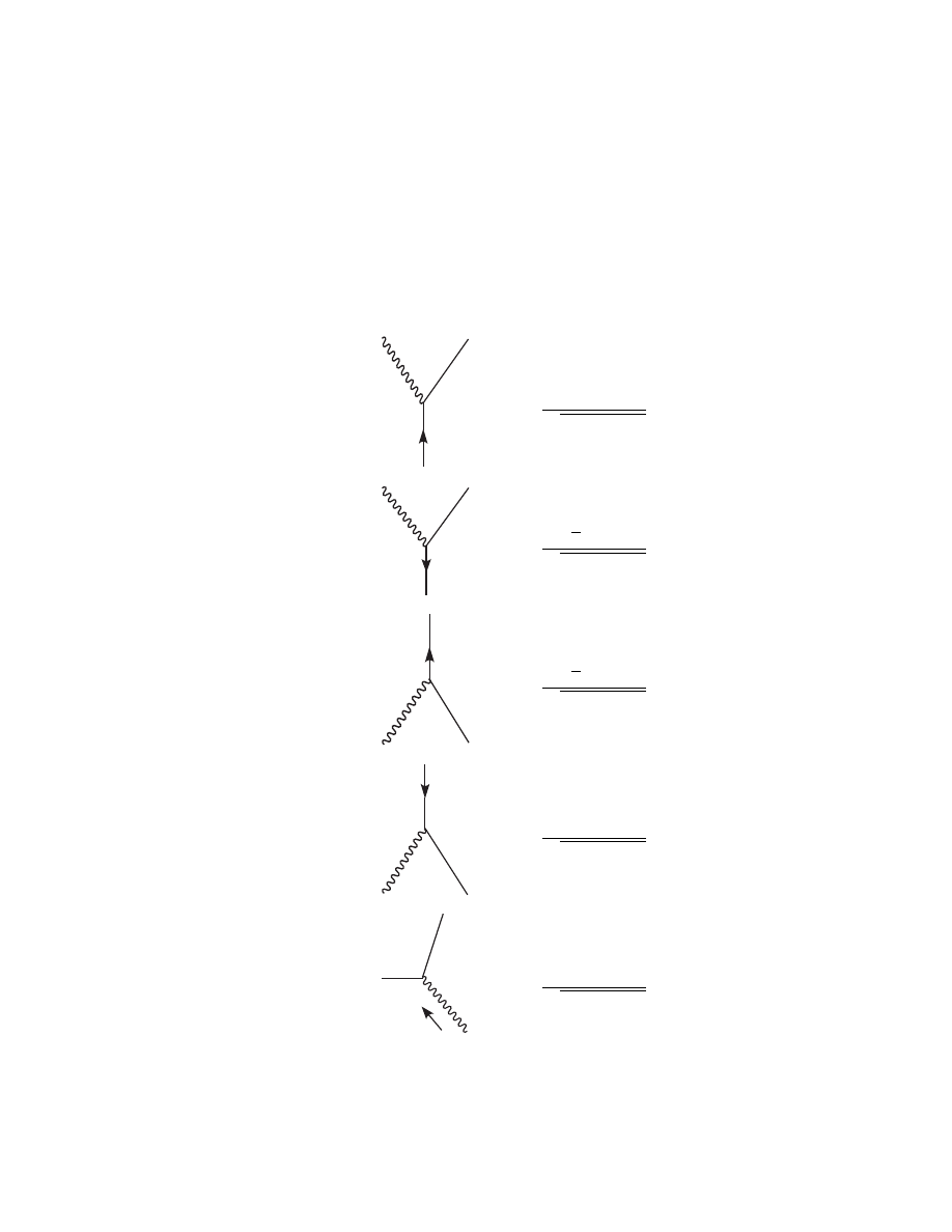
8.3. FEYNMAN’S RULES FOR QED
133
1. Draw all possible connected, topologically distinct diagrams, including
loops, with n external legs. Ignore vacuum-to-vacuum graphs. Each
vertex must have a continuous electron or positron line and a photon
line terminating on the fermion.
2. There is a factor given by the following rules for each external line.
Incoming fermion:
p
=
u(p, s)
p
Z
2
(2π)
3
2E
p
Incoming antifermion:
p
=
v(p, s)
p
Z
2
(2π)
3
2E
p
Outgoing fermion:
p
=
u(p, s)
p
Z
2
(2π)
3
2E
p
Outgoing antifermion:
p
=
v(p, s)
p
Z
2
(2π)
3
2E
p
Incoming photon:
p
=
²
µ
(p)
p
Z
3
(2π)
3
2E
p
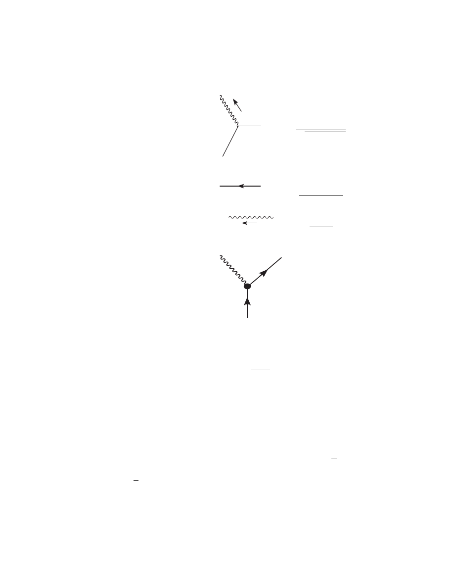
134
CHAPTER 8. QUANTUM ELECTRODYNAMICS
Outgoing photon:
p
=
²
µ∗
(p)
p
Z
3
(2π)
3
2E
p
3. For each internal line there is a propagator
Electron propagator:
p
=
i(6 p + m)
p
2
− m
2
+ i²
Photon propagator:
p
µ
ν
=
−ig
µν
p
2
+ i²
4. At each vertex, place a factor of −ieγ
µ
.
Electron-photon vertex:
= −ieγ
µ
5. Insert an additional factor of -1 for each closed fermion loop.
6. For each internal loop, integrate over:
Z
d
4
q
(2π)
4
(8.34)
7. A relative factor -1 appears between graphs that differ from each other
by an interchange of two identical external fermion lines.
8. Internal fermion lines appear with arrows in both clockwise and coun-
terclockwise directions. However. diagrams that are topologically
equivalent are counted only once.
Remember that the electron-photon coupling has the form eψγ
µ
ψA
µ
. As
a consequence, the spinors associated with any vertex must appear in the
order uγ
µ
u (with v replacing u as needed).
With this in mind, let’s do some examples.

8.4. THE REACTION E
−
+ E
+
→ µ
−
+ µ
+
135
8.4
The Reaction e
−
+ e
+
→ µ
−
+ µ
+
Consider the reaction e
−
+ e
+
→ µ
−
+ µ
+
. In terms of momentum, that is
p + p
0
→ k + k
0
, and in terms of spin indices we have s and s
0
→ r and r
0
.
The momentum of the exchanged photon is q = p + p
0
= k + k
0
. The muons
are almost identical to electrons, i.e. they have the same electromagnetic
interactions, but they are heavier by a factor of 200. This simplifies the
problem in several ways. For one thing, we are usually entitled to neglect
the mass of the electron. For another, there are no identical particles in this
example. Feyman’s rules give
iM =
ie
2
q
2
¡
v
e
(p
0
)γ
µ
u
e
(p)
¢ ¡
u
µ
(k)γ
µ
v
µ
(k
0
)
¢
(8.35)
I have added subscripts e and µ to the spinors to indicate that they contain
different masses. The spin indices are implicit. I will get back to spins in a
minute.
In order to obtain a differential cross section from M we must do three
difficult things: square it, sum over final spins, and average over initial spins.
In order to make the notation more compact, I will write (8.35) as
iM =
ie
2
q
2
a
µ
b
µ
(8.36)
In order to calculate |M |
2
, we will need to figure out
|ab|
2
= a
µ
a
ν†
b
µ
b
†
ν
(8.37)
Notice that a and b are 1 × 1 matrices in spin space and four-vectors in
Minkowski space. There are two useful consequences; they all commute and
complex conjugation and Hermitian conjugation have the same effect. This
allows us to write
a
ν†
= u
†
γ
ν†
γ
0†
v = u
†
γ
0
γ
ν
v = uγ
ν
v
(8.38)
With that insight (8.37) becomes
|M |
2
=
e
4
q
4
¡
v(p
0
)γ
µ
u(p)u(p)γ
ν
v(p
0
)
¢ ¡
u(k)γ
µ
v(k
0
)v(k
0
)γ
ν
u(k)
¢
(8.39)
Now make use of the spin information. The differential cross section will be
proportional to
1
2
X
s
1
2
X
s
0
X
r
X
r
0
|M (s, s
0
, r, r
0
)|
2
(8.40)

136
CHAPTER 8. QUANTUM ELECTRODYNAMICS
Remember from a previous chapter
X
s
u(p, s)u(p, s) =
6 p + m
2m
(8.41)
X
s
v(p, s)v(p, s) =
6 p − m
2m
Let’s do the spin sums on the first term of (8.39)
X
s,s
0
v(p
0
, s
0
)γ
µ
u(p, s)u(p, s)γ
ν
v(p
0
, s
0
)
(8.42)
=
1
2m
X
s
0
v
a
(p
0
, s
0
)γ
µ
ab
(6 p + m)
bc
γ
ν
cd
v
d
(p
0
, s
0
)
I apologize for the notational overload. An object like γ
µ
is a 4 × 4 matrix
in spin space. I have turned it in to a tensor by adding the matrix indices
a and b. Tensors commute as you know, so (8.42) can be rewritten
=
1
2m
X
s
0
v
d
(p
0
, s
0
)v
a
(p
0
, s
0
)γ
µ
ab
(6 p + m)
bc
γ
ν
cd
Now v and v are in the right relation to one another so that we can use
(8.41)
=
µ
1
2m
¶
2
(6 p
0
− m)
da
γ
µ
ab
(6 p + m)
bc
γ
ν
cd
Now this is recognizable as the trace of a product of matrices.
=
µ
1
2m
¶
2
Tr
£
(6 p
0
− m)γ
µ
(6 p + m)γ
ν
¤
Finally combining (8.39), (8.40), and (8.42), we get
1
4
X
spins
|M |
2
=
1
4
µ
e
2mq
¶
4
Tr
£
(6 p
0
− m
e
)γ
µ
(6 p + m
e
)γ
ν
¤
× Tr
£
(6 p
0
− m
µ
)γ
µ
(6 p + m
µ
)γ
ν
¤
(8.43)
There you have it. QED calculations eventually come down to taking traces.

8.4. THE REACTION E
−
+ E
+
→ µ
−
+ µ
+
137
8.4.1
Trace Technology
The things we are taking traces of are all 4 × 4 matrices, even when they
don’t look like that. This results in some paradoxical formulas like Tr 1 = 4
and Tr m = 4m. You can check from the representation of the gamma
matrices that Trγ
µ
= 0. Traces of an even number of γ’s are generally not
zero. Here is a simple result.
Tr(6 a 6 b) = a
µ
b
ν
Tr(γ
µ
γ
ν
) =
1
2
a
µ
b
ν
Tr{γ
µ
, γ
ν
} = a
µ
b
ν
Tr(g
µν
) = 4a · b
I have used the important fact that the trace of a product of matrices such as
Tr(abc · · · z) is invariant under any cyclic permutation of the matrices. Thus
in the equation above Tr(γ
µ
γ
ν
) = Tr(γ
ν
γ
µ
). Our result can be summarized
Tr(γ
µ
γ
ν
) = 4g
µν
(8.44)
The trace of an odd number of γ’s always vanishes. The proof requires
a trick. Remember the γ
5
matrix. It has the properties
Tr(γ
5
) = 0
(γ
5
)
2
= 1
{γ
5
, γ
µ
} = 0
Now the line of argument goes
Tr(6 a
1
6 a
2
· · · 6 a
n
) = Tr(6 a
1
6 a
2
· · · 6 a
n
γ
5
γ
5
) = Tr(γ
5
6 a
1
6 a
2
· · · 6 a
n
γ
5
)
= (−1)
n
Tr(6 a
1
6 a
2
· · · 6 a
n
γ
5
γ
5
) = (−1)
n
Tr(6 a
1
6 a
2
· · · 6 a
n
)
The trace is zero for n odd.
There are many other identities that are easily proved. In a moment I
will use
Tr(γ
µ
γ
ν
γ
ρ
γ
σ
) = 4(g
µν
g
ρσ
− g
µρ
g
νσ
+ g
µσ
g
νρ
)
(8.45)
which is obtained from repeated application of (8.44). Others can be found
in any standard text. At the moment I am looking at Peskin and Schroder,
Introduction to Quantum Field Theory Appendix A3.
8.4.2
Kinematics
A short calculation using (8.45) yields
Tr
£
(6 p
0
− m)γ
µ
(6 p + m)γ
ν
¤
= 4[p
0µ
p
ν
+ p
0ν
p
µ
− g
µν
(p · p
0
+ m
2
e
)]
(8.46)
We can set m
2
e
= 0. Then (8.43) can be evaluated by using (8.46) twice.
1
4
X
spins
|M |
2
=
8e
4
q
4
[(p · k)(p
0
· k
0
) + (p · k
0
)(p
0
· k) + m
2
µ
(p · p
0
)]
(8.47)

138
CHAPTER 8. QUANTUM ELECTRODYNAMICS
Equation (8.47) is valid in any Lorentz frame. This is fine as far as it
goes, but in order to compare the result with an experiment, we need to
specialize to a definite frame of reference. Such an experiment is typically
done with a colliding beam machine for which the laboratory is the CM
frame. Let us assume then that k = (E, k), k
0
= (E, −k), p = (E, E ˆ
z) and
p
0
= (E, −E ˆ
z). The angle between k and the z axis is θ. The following
kinematic identities follow with m
e
= 0.
q
2
= (p + p
0
)
2
= 4E
2
p · p
0
= 2E
2
p · k = p
0
· k
0
= E
2
− E|k| cos θ
p
0
· k = p · k
0
= E
2
+ E|k| cos θ
Eqn. (8.47) can be rewritten
1
4
X
spins
|M |
2
= e
4
"Ã
1 +
m
2
µ
E
2
!
+
Ã
1 −
m
2
µ
E
2
!
cos
2
θ
#
(8.48)
Back in Chapter 8 I derived the relationship between M and the differ-
ential cross section. Since then we have introduced the Dirac spinors, which
must be normalized differently from the Kline-Gordon fields. I will therefore
state (without proof) the appropriate version of ?? is
µ
dσ
dΩ
¶
CM
=
1
2E
A
E
B
|v
A
− v
B
|
|p
1
|
(2π)
2
4E
CM
|M (p
A
+ p
B
→ p
1
+ p
2
)|
2
(8.49)
This holds in any coordinate system in which generic particles A and B
scatter into a final state consisting of two particles with momenta p
1
and
p
2
. In our case particles A and B are collinear and assumed massless. In
this case
|v
A
− v
B
| =
¯
¯
¯
¯
k
A
E
A
−
k
B
E
B
¯
¯
¯
¯ = 2
(8.50)
In our example the M in (8.49) is replaced by the spin-averaged M of (8.48).
8.5
Introduction to Renormalization
Every Feynman diagram with one or more closed loops yields a divergent in-
tegral.
3
One of the most important discoveries of twentieth-century physics
is that these divergent terms contain real physical content that is part of
3
There are some exceptions in the case of spin-zero particles, but it’s universally true
in qed.

8.5. INTRODUCTION TO RENORMALIZATION
139
the “right answer” to any higher-order calculation. The program of extract-
ing useful information from meaningless infinities is called renormalization.
This is an extremely technical and complicated subject, but I would like
to expose you to some of the basic ideas. To do this, I will concentrate
on a subset of divergent diagrams that go under the heading of electron
self-energy.
Consider the quantum process in which a single photon of momentum
k is emitted and reabsorbed by a virtual electron with initial and final mo-
mentum p. In the interim between emitting and reabsorbing the photon the
electron has momentum q = p − k. According to Feynman’s rules, Section
11.3, the amplitude for this process is
iS
F
(p)
Z
d
4
k
(2π)
4
(−ieγ
µ
)
µ
−ig
µν
k
2
+ i²
¶
i(6 p− 6 k + m)
(p − k)
2
− m
2
+ i²
(−ieγ
ν
)iS
F
(p)
(8.51)
= iS
F
(p)
·
−ie
2
Z
d
4
k
(2π)
4
γ
µ
(m+ 6 p− 6 k)γ
µ
(−k
2
− i²)(m
2
− (p − k)
2
− i²)
¸
S
F
(p)
≡ iS
F
(p)Σ(p)S
F
(p)
The last equality implicitly defines the divergent quantity Σ, know as a
“self-energy insertion.” It is clearly divergent, since there are five powers of
k in the numerator and only four in the denominator. We will eventually
evaluate it, but for the time being I would like to investigate some of its
general properties. Such as term would arise in perturbation theory as a
second-order correction to the electron propagator. We could define a “more
nearly exact” propagator
iS
0
F
(p) ≈ iS
F
(p) + iS
F
(p)Σ(p)S
F
(p)
I say “more nearly exact” meaning that iS
0
F
(p) contains all the second-
order corrections that would arise in the usual perturbation expansion of
the propagator. We could make an even better approximation by including
another self-energy insertion.
iS
0
F
≈ iS
F
+ iS
F
ΣS
F
+ iS
F
ΣS
F
ΣS
F
This is not quite correct, even to fourth order, since I have ignored the dia-
gram in which the electron emits another photon before reabsorbing the first.
Diagrams of this sort are called “overlapping divergences.” Such diagrams
present a huge additional complication, but “sufficient unto the day is the
evil thereof.” I will ignore them. My conclusions will still be qualitatively
correct.

140
CHAPTER 8. QUANTUM ELECTRODYNAMICS
I can go on adding diagrams like this ad infinitum. The sum would look
like this.
iS[1 + ΣS + ΣSΣS + (ΣS)
3
+ · · · ]
(8.52)
(I have suppressed the F subscript and well as the (p) to make the equations
easier to read.) This looks like the familiar geometric series (1 − x)
−1
=
1 + x
2
+ x
3
+ · · · , so I am tempted to write
iS
0
= iS
1
1 − ΣS
(8.53)
The question is, what does it mean to divide by a 4 × 4 matrix? You can
regard (8.53) as notational shorthand for (8.52). Here are some further
observations.
• It’s clear from (8.52) that Σ has the form
Σ = mA(p
2
)+ 6 pB(p
2
)
(8.54)
It’s true that A and B are infinite, but let’s ignore that for the time
being. Furthermore
S =
6 p + m
p
2
− m
2
(I will ignore the i²’s for the time being also. I don’t want to distract
you with details. I promise I haven’t forgotten them and will put
them back when necessary.) It follows that [S, Σ] = 0. Therefore the
following forms are equivalent.
S
0
= S
1
1 − ΣS
=
1
1 − ΣS
S =
S
1 − ΣS
(8.55)
• Since 6 p 6 p = p
2
it makes sense to write in the same spirit
S =
6 p + m
p
2
− m
2
=
6 p + m
(6 p − m)(6 p + m)
=
1
6 p − m
,
(8.56)
and finally
S
−1
=6 p − m.
(8.57)
The propagator can now be rewritten
iS
0
=
iS
1 − ΣS
S
−1
S
−1
=
i
6 p − m − Σ
(8.58)

8.5. INTRODUCTION TO RENORMALIZATION
141
Leaving aside the fact that Σ is infinite, there is still a strange pathology
in (8.57). Every propagator we have encountered so far has had a pole at
the mass of the particle. It is almost axiomatic that a propagator is the
probability amplitude for the particle to propagate from x to y such that
p
2
= m
2
on the mass shell. It must be that the series of self-energy terms we
have summed has modified the mass of the particle. We have to confess that
at least in the context of perturbation theory, the m that appears in the
Hamiltonian is not the physical mass of the particle. We call the m in the
Hamiltonian the “bare” mass and the mass that marks the pole of the exact
propagator, the “dressed” or physical mass, which I will call m. It seems
that given the bare mass, we should be able to calculate the physical mass
or vice versa. The fact that Σ is infinite makes this permanently impossible.
We have not faced up to this problem so far, because we have always worked
at the lowest non-trivial order of perturbation theory. To that order we can
assume the the bare and physical masses are identical, and everything works
out OK. As soon as we include the self-energy terms, we must keep track
of both m and m. Worse yet, the same sort of thing happens when we
calculate higher-order corrections to the electron-photon vertex. There we
find that the charge e put into the Hamiltonian is not the physical charge of
the electron but some “bare” charge, and again we must keep track of the
e’s and e’s.
The agenda of keeping track of these corrections goes by the name “renor-
malization.” It is a remarkable fact that all the infinite corrections brought
about by all loop diagrams to all orders of perturbation theory can swept un-
der the rug of these two constants. A theory for which this is possible is said
to be “renormalizable.” It is an article of faith that no non-renormalizable
theory can be completely right, however useful it might be phenomenologi-
cally. Fermi’s theory of weak interactions, which we will study in the next
chapter, is a good example. It explains nuclear beta decay quite nicely, but
it would require an infinite number of infinite constants to take care of all
the loops! It was eventually modified by the addition of the intermediate
vector bosons. The resulting theory is called the “standard model.” It is
renormalizable and right! It is also possible to do quantum field theory with
gravitons. The theory at least predicts Newton’s law of gravitation. To this
extent it is correct. It is non-renormalizable, however, and we have no idea
what the true theory might be.
It is necessary to rewrite (8.58) in such a way that the physical mass
appears in the denominator. To this end we expand the self energy term as
follows.
Σ(6 p) = Σ(m) + (6 p − m)Σ
0
(m) + (6 p − m)
2
R(p
2
)
(8.59)

142
CHAPTER 8. QUANTUM ELECTRODYNAMICS
This is the key equation, and it deserves some comment.
• It looks like a power series expansion about the point 6 p = m, but in
fact, 6 p can never equal m, since m is diagonal and 6 p never is. Rather,
(8.59) defines implicitly what is meant by R(p
2
). I will sometimes
write it
Σ(6 p) = Σ(m) + (6 p − m)Σ
0
(m) + Σ
R
(6 p)
(8.60)
In which case it defines Σ
R
. By construction Σ
R
(m) = 0.
• It appears that in the term Σ
0
we have differentiated with respect to a
matrix! That is not so strange as it seems. The point is that p
2
=6 p
2
.
For example, the A(p
2
) term in (8.54) can be differentiated as follows.
A
0
(m) =
dA(p
2
)
d 6 p
¯
¯
¯
¯
6p=m
=
dA(p
2
)
dp
2
d 6 p
2
d 6 p
¯
¯
¯
¯
6p=m
= 2m
dA(p
2
)
dp
2
¯
¯
¯
¯
p
2
=m
2
(8.61)
Strictly speaking, Σ(m) and Σ
0
(m) are both infinite, so the operations
in (8.60) and (8.61) are not well defined. Our strategy for giving them a
precise meaning works as follows. I will introduce an additional parameter
² into (8.51) in such a way the the integrals converge for ² > 0. It will turn
out that A(p
2
) and B(p
2
) in (8.54) can each be split into two parts. One
part will depend on ². It becomes infinite as ² → 0, but for ² 6= 0 it is
a well-behaved mathematical expression. The other part will depend on p
2
but not on ². It is finite, calculable, and important. I am about to show that
all the epsilon-dependent terms can be lumped together with the bare mass
to give the physical mass m and a new epsilon-dependent term Z
2
called
the wave function renormalization factor, which cancels out in any complete
calculation of a Feynman diagram. The point is that all these calculations
are done with finite (though epsilon-dependent) terms, and when the time
comes to calculate some physical quantity such as a cross section or reaction
rate, there are no epsilon-dependent terms remaining.
Now substitute (8.60) into (8.58)
iS
0
=
−i
m + Σ(m)− 6 p + (6 p − m)Σ
0
(m) + Σ
R
(8.62)
I looks like the “real” mass is m = m+Σ(m). We need one further constant.
4
Z
−1
2
≡ 1 − Σ
0
(m)
(8.63)
4
This is standard notation. There are other Z’s, but since we are only dealing with
the electron self-energy part, these other constants don’t arise.

8.5. INTRODUCTION TO RENORMALIZATION
143
Equation (8.62) can be rewritten
iS
0
=
i(6 p + m)
p
2
− m
2
Z
2
1 + (m− 6 p)Z
2
R(p
2
)
(8.64)
The looks like the “bare” propagator iS (with m replaced by m) multiplied
by a factor, which, if Z
2
were not epsilon-dependent, would be finite and
calculable. Before we set ² = 0, however, Z
2
is finite, and we can show why it
does not appear in the final result of any complete calculation of a Feynman
diagram. First consider the Z
2
in the denominator of (8.64). You can see
from (8.51) that Σ is proportional to e
2
. We must confess again the the e
that appears in the Hamiltonian is not the measured charge of the electron,
but rather a “bare” charge, which is modified by all the loop diagrams to all
orders of perturbation theory. Part of this modification is due to Z
2
. Let’s
tentatively define a “dressed” charge, e =
√
Z
2
e. Then Z
2
disappears from
the denominator because it is absorbed into Σ. The Z
2
disappears from the
numerator when we realize that our virtual electron will not be observable
until it couples to a photon at each end. (Draw some Feynman diagrams
to convince yourself this is true.) Each electron-photon vertex comes with
a factor of e, so the entire diagram is proportional to e
2
Z
2
= e
2
.
Now I will evaluate the very difficult integral (8.51). Notice that the
denominator is the product of two factors that can be labelled
A = m
2
− (p − k)
2
− i²
B = −k
2
− i²
Feyman realized that a four-dimensional integral can be simplified by making
it five-dimensional. The trick is
1
AB
=
Z
1
0
dz
[Az + B(1 − z)]
2
≡
Z
1
0
dz
D
2
(8.65)
The term D can be simplified by completing the square. Define k
µ
≡ k
0µ
+
zp
µ
. Then
D = C
2
− k
02
where
C
2
≡ z[m
2
− p
2
(1 − z)]
With these substitutions, the numerator of (8.51) becomes
N (p, z) = γ
µ
[m+ 6 p(1 − z)− 6 k
0
]γ
µ
I can delete the 6 k
0
term using the familiar argument that an odd function
integrated over even limits yields zero. Using the fact that γ
µ
γ
µ
= 4, gives
us the final form of the numerator function.
N = 2[2m− 6 p(1 − z)]
(8.66)

144
CHAPTER 8. QUANTUM ELECTRODYNAMICS
With all these definitions the self-energy term becomes
Σ(p) = −ie
2
Z
1
0
dzN (p, z)
Z
d
4
k
(2π)
4
1
(C
2
− k
2
− i²)
2
(8.67)
The integral can be done for integer dimension d using the remarkable for-
mula
5
Z
d
d
k
(2π)
d
1
(C
2
− k
2
− i²)
n
=
i
(4π)
d/2
Γ(n − d/2)
Γ(n)
µ
1
C
2
¶
n−d/2
(8.68)
Here Γ is the Euler gamma function defined by
Γ(α) ≡
Z
∞
0
dt t
α−1
e
−t
(8.69)
If α is an integer, say n, Γ(n) = (n−1)!, and in general Γ(α) = (α−1)Γ(α−1).
It’s useful to get Maple to plot this function for you. You will see that Γ
interpolates smoothly between the integer values of α. You will also see
that Γ(0) = ∞. We expected that. The integral (8.67) has to diverge. Now
of course, the integral on the left side of (8.68) only makes sense when d
is an integer, but the expression on the right interpolates smoothly between
integer values of d. Even if d is only infinitesimally less than four, it is still
finite. Now define ² ≡ 4 − d. For our purposes, n = 2.
Γ(n − d/2)
Γ(n)
=
Γ(3 − d/2)
2 − d/2
=
2
²
Σ(p) =
2e
2
(4π)
2
Z
1
0
dzN
C
−²
²
(8.70)
Insert the expansion
C
−²
= 1 − ² ln C + O(²
2
)
Σ(p) =
2e
2
(4π)
2
Z
1
0
dzN (6 p, z)
µ
1
²
− ln C(p
2
, z)
¶
+ O(²)
(8.71)
The integrals in (8.71) are easy enough to do, although the resulting expres-
sions are not very illuminating. The important point is that Σ(6 p) can be
divided up as follows.
Σ(6 p) = (mB
1
+ 6 pB
2
)/² + ˜
Σ(6 p)
(8.72)
5
This is proved in Gross, Relativistic Quantum Mechanics and Field Theory, page 344

8.5. INTRODUCTION TO RENORMALIZATION
145
where ˜
Σ(6 p) does not contain ² and so remains finite in the limit ² → 0. B
1
and B
2
are simple constants. When we expand Σ(6 p) using (8.60), Σ
R
(6 p)
is as promised, finite. Thus we can absorb all the infinite terms into the
two constants m and Z
2
, and calculate Σ
R
(6 p)and R(p
2
) which are, again as
promised, finite and important.
Wyszukiwarka
Podobne podstrony:
Modanese Inertial Mass and Vacuum Fluctuations in Quantum Field Theory (2003)
Seahra S Path integrals in quantum field theory (web draft, 2002)(36s) PQft
Alvarez Gaume L , Introductory Lectures on Quantum Field Theory
Srednicki M Quantum field theory, part 2 spin one half (web draft, 2005)(146s) PQtb
Norbury Quantum field theory (Wisconsin lecture notes, 2000)(107s)
Classical Field Theory Janos Polonoi
An Introduction to Conformal Field Theory [jnl article] M Gaberdiel (1999) WW
Selfridge, Arnold, Warnick Teaching Electromagnetic Field Theory Using Differential Forms (IEEE Tran
NLP Beyond words languaging change thru the quantum field
Haisch et al Advances in the Proposed Electromagnetic Zero Point Field Theory of Inertia (1998)
Girotti H O Noncommutative quantum field theories (Swieca lectures, Sao Paolo, 2003) (58s)
Lasenby et al Multivector Derivative Approach 2 Lagrangian Field Theory (1993) [sharethefiles com]
Field M , Nicol M Ergodic theory of equivariant diffeomorphisms (web draft, 2004)(94s) PD
General Relativity Theory, Quantum Theory of Black Holes and Quantum Cosmology
Escobedo M , Mischler S , Valle M A Homogeneous Boltzmann equation in quantum relativistic kinetic t
Feynman s Path Integral in Quantum Theory
Interpretation of quantum mechanics by the double solution theory by Louis de Broglie
Hardy L quant ph 0101012 Quantum Theory From Five Reasonable Axioms (2001) (34s)
więcej podobnych podstron