
ANALYSIS AND DETECTION OF METAMORPHIC
COMPUTER VIRUSES
A Writing Project
Presented to
The Faculty of the Department of
Computer Science
San Jose State University
In Partial Fulfillment
Of the Requirements for the Degree
Master of Science
By
Wing Wong
May, 2006

Approved by:
Department of Computer Science
College of Science
San Jose State University
San Jose, CA
_______________________________
Dr. Mark Stamp
_______________________________
Dr. Robert Chun
_______________________________
Dr. Suneuy Kim

i
Acknowledgements
I would like to thank my advisor Dr. Mark Stamp for his guidance and patience. Without
his insights, feedbacks, and encouragement, this project would not have been a success. I
would also like to express my thanks to the following professors. Dr. Sami Khuri
introduced me to hidden Markov models when I first started my graduate studies at San
Jose State University. Dr. Kevin Karplus gave me the chance to work with his lab group
at UC Santa Cruz, where I learned how
to utilize the magnificent power of hidden
Markov models to solve practical problems. Dr. Chris Pollett provided me with valuable
comments during the formulation of the project topic. Dr. Robert Chun suggested the
comparison between our
approach and
commercial virus scanners.
I would also like to thank my friends and schoolmates for their technical and emotional
support. I want to thank Yue Wang for performing the virus scanning, and Peter Hey for
repairing my hard disk after it crashed
at the most critical moment.
Finally I want to thank my family for their understanding and support throughout my five
years of graduate studies. They have shown the greatest care and patience which I truly
appreciate.

ii
Abstract
Computer virus writers commonly use metamorphic techniques to produce viruses that
change their internal structure on each infection. It is generally believed that these
metamorphic viruses are extremely difficult to detect. Metamorphic virus generating kits
are readily available, so that little knowledge or skill is required to create these
potentially devastating viruses.
In this project, we first analyze four virus creation kits to determine the degree of
metamorphism provided by each. We are able to precisely quantify the degree of
metamorphism produced by these virus generators. While the best generator, the Next
Generation Virus Creation Kit (NGVCK), produces virus variants that differ greatly from
one another, the other three generators we examined are much less effective.
We then show that three popular commercial virus scanners cannot detect any of the
NGVCK viruses in our test set. We proceed to develop an effective metamorphic virus
detection technique based on hidden Markov models (HMM). With this HMM detector,
we are able to classify a given program as belonging to a particular virus family or not.
Using this approach, we can detect all metamorphic viruses in our test set with extremely
high accuracy. We also present a simpler detection method that detects metamorphic
viruses with high accuracy.
Our results show that the best available metamorphic generator is effective at morphing
viral code and that the resulting morphed viruses are not detectable using popular
commercial virus scanning software. Surprisingly, these viruses differ sufficiently from
non-viral code so that they are detectable using a similarity technique that we present in
this paper. It remains an interesting open question whether metamorphic viral code can be
constructed which is undetectable using our techniques.

iii
Table of Contents
1. INTRODUCTION..................................................................................................... 1
2. EVOLUTION OF VIRUSES AND ANTIVIRUS DEFENSE TECHNIQUES... 2
2.1
Virus Obfuscation Techniques ....................................................................................2
2.1.1
Encrypted Viruses ...................................................................................................................3
2.1.2
Polymorphic Viruses ...............................................................................................................3
2.1.3
Metamorphic Viruses ..............................................................................................................4
2.1.4
Virus Construction Kits...........................................................................................................6
2.2
Antivirus Defense Techniques .....................................................................................7
2.2.1
First Generation Scanners........................................................................................................8
2.2.2
Second Generation Scanners ...................................................................................................8
2.2.3
Code Emulation.......................................................................................................................9
2.2.4
Heuristic Analysis .................................................................................................................10
2.3
Use of Machine Learning Techniques ......................................................................10
2.3.1
Data Mining Approach ..........................................................................................................10
2.3.2
Neural Networks....................................................................................................................11
2.3.3
Hidden Markov Models.........................................................................................................12
3. SIMILARITIES BETWEEN VARIANTS OF METAMORPHIC VIRUSES . 13
3.1
Method to Compare Two Pieces of Code .................................................................13
3.2
Test Data .....................................................................................................................15
3.3
Test Results .................................................................................................................17
4. HIDDEN MARKOV MODELS TO DETECT VIRUSES IN SAME FAMILY25
4.1
Theory and Algorithms for Hidden Markov Models ..............................................25
4.1.1
Notation.................................................................................................................................27
4.1.2
Algorithms.............................................................................................................................31
4.1.2.1
Finding the likelihood of an observation sequence: the Forward algorithm ................31
4.1.2.2
Finding the most likely state sequence: the Viterbi algorithm .....................................33
4.1.2.3
Finding the optimal model parameters: the Baum-Welch algorithm ...........................34
4.1.2.4
Posterior state probabilities..........................................................................................39
4.1.3
Implementation Issues: Underflow and Scaling ....................................................................39

iv
4.2
HMM for Computer Virus Detection .......................................................................42
4.3
Training and Testing..................................................................................................44
4.4
Data Used ....................................................................................................................46
4.5
Experimental Results .................................................................................................48
4.5.1
Separation of Scores ..............................................................................................................48
4.5.2
Threshold and False Predictions............................................................................................53
4.5.3
Detection Rate, False Positive Rate, and Overall Accuracy..................................................55
4.5.4
Run Time of the Training and Classifying Process ...............................................................58
4.6
The Trained Models ...................................................................................................60
5. DETECTION WITH SIMILARITY INDEX AND COMMERCIAL
SCANNERS..................................................................................................................... 64
5.1
Classifying by Similarity Index .................................................................................64
5.2
Detection by Virus Scanners......................................................................................67
6. CONCLUSION ....................................................................................................... 69
7. FUTURE WORK.................................................................................................... 72
Bibliography .................................................................................................................... 74
Appendix A: Virus similarity test results ..................................................................... 76
Appendix B: HMM training and testing results .......................................................... 82
Appendix C: Converged HMM matrices...................................................................... 94
Appendix D: Detection using similarity index ........................................................... 100

v
List of Figures
Figure 1 Multiple shapes of a metamorphic virus body [20]............................................. 4
Figure 2 Zperm virus [19].................................................................................................. 5
Figure 3 Process of finding the similarity between two assembly programs. ................. 15
Figure 4 Scatter plot showing similarity scores between NGVCK virus variants and
between normal files................................................................................................. 17
Figure 5 Bubble graph showing minimum, maximum, and average similarity between
virus variants generated by each generator and between normal files...................... 19
Figure 6 Minimum, maximum, and average similarities between NGVCK virus variants,
between NGVCK viruses and VCL32 viruses, and between NGVCK viruses and
normal files. .............................................................................................................. 25
Figure 7 A generic hidden Markov model [18]. .............................................................. 28
Figure 8 Inductive process of finding
t
(i) from variables
t-1
(j). ................................... 32
Figure 9 Inductive process of finding
t
(i) from variables
t+1
(j).................................... 35
Figure 10 Variables for the computation of the joint probability
t
(i, j).......................... 37
Figure 11 Training and classifying process. .................................................................... 46
Figure 12 Difference in scores between family viruses and normal files........................ 50
Figure 13 Log likelihood per opcode (LLPO) of family viruses, non-family viruses and
normal files. .............................................................................................................. 52
Figure 14 Tradeoff between false positives (FP) and false negatives (FN) with changing
threshold values. ....................................................................................................... 54
Figure 15 Comparison of false positive rate, detection rate and overall accuracy. ......... 56
Figure 16 Training time of the 25 models using 500 iterations and 800 iterations
respectively. .............................................................................................................. 59
Figure 17 Scoring time as a function of observation sequence length T and number of
states N...................................................................................................................... 60

vi
Figure 18 Probability distributions of observation symbols for each state in the model
with N = 3 using test set 0......................................................................................... 63
Figure 19 Probabilities of each opcode in state 0, state 1, and state 2 normalized to show
the composition of states for each opcode. ............................................................... 64
Figure 20 Screen capture of the eTrust scanning result on the 37 virus executables. ..... 68
Figure 21 Test result for AVG Anti-Virus on the 37 virus executables. ......................... 69

vii
List of Tables
Table 1 Minimum, maximum, and average similarity scores between virus variants
generated by the generators and between normal files ............................................. 18
Table 2 Similarity graphs of four selected virus pairs and one normal file pair.............. 21
Table 3 Similarity graphs of the NGVCK virus pair that has the highest similarity....... 22
Table 4 Similarity graphs showing similarity between IDA_NGVCK0 and IDA_VCL4
................................................................................................................................... 23
Table 5 The eight pairs of NGVCK viruses and normal files that have non-zero
similarity scores ........................................................................................................ 24
Table 6 Probabilities of observing O = (0, 1, 0, 2) for all possible 4-state sequences..... 30
Table 7 LLPO scores of the 40 family viruses in test set 0 and the 40 normal files using
the model with N = 2 ................................................................................................ 49
Table 8 Minimum score of the 40 family viruses and maximum score of the 40 normal
programs assigned by each model ............................................................................ 51
Table 9 False positive (FP) and false negative (FN) counts for threshold ranging from -
3.5 to -2.5 .................................................................................................................. 55
Table 10 Threshold LLPO with detection rate of 90% or more for each model ............. 57
Table 11 False positive count, false negative count, detection rate, false positive rate and
overall accuracy when threshold is set at -4.5 for all models ................................... 58
Table 12 The final B matrix transpose for model with N = 3 using test set 0 ................. 62
Table 13 Similarity scores between IDA_N146 and other programs including NGVCK
viruses, non-NGVCK viruses, and normal programs ............................................... 66
Table A-1 Similarity scores between NGVCK virus variants......................................... 76
Table A-2 Similarity scores between G2 virus variants .................................................. 77
Table A-3 Similarity scores between VCL32 virus variants ........................................... 78
Table A-4 Similarity scores between MPCGEN virus variants....................................... 79

viii
Table A-5 Similarity scores between random normal files ............................................. 80
Table A-6 Similarity scores between NGVCK virus and VCL32 virus pairs that have
score greater than 0 ................................................................................................... 81
Table B-1 LLPO of family viruses, non-family viruses and normal files with N = 3..... 82
Table B-2 LLPO of family viruses, non-family viruses and normal files with N = 5..... 85
Table B-3 Raw LLPO scores of all 105 programs returned by the 25 HMMs................ 88
Table C-1 Final (A, B, ) for model with N = 3 states using test set 0 ........................... 94
Table C-2 Final (A, B, ) for model with N = 3 states using test set 2 ........................... 95
Table C-3 Final (A, B, ) for model with N = 3 states using test set 4 ........................... 96
Table C-4 Final (A, B, ) for model with N = 5 states using test set 0 ........................... 97
Table C-5 Final (A, B, ) for model with N = 5 states using test set 2 ........................... 98
Table C-6 Final (A, B, ) for model with N = 5 states using test set 4 ........................... 99
Table D-1 Similarity scores between IDA_N101 and other programs including NGVCK
viruses, non-NGVCK viruses, and normal programs ............................................. 100

1
1. INTRODUCTION
“A computer virus is a program that recursively and explicitly copies a possibly evolved
version of itself” [19]. A virus copies itself to a host file or system area. Once it gets
control, it multiplies itself to form newer generations. A virus may carry out damaging
activities on the host machine such as corrupting or erasing files, overwriting the whole
hard disk, or crashing the computer. Some viruses may print text on the screen or simply
do nothing. These viruses remain harmless but keep reproducing themselves. In any case,
viruses are undesirable for computer users.
Over the past two decades, the number of viruses has been increasing rapidly. We have
seen several attacks that caused great disruption to the Internet and brought huge damage
to organizations and individuals. For example, in 1999, the infamous Melissa virus
infected thousands of computers and caused damage close to $80 million; while the Code
Red worm outbreak in 2001 affected systems running Windows NT and Windows 2000
server and caused damage in excess of $2 billion [23]. Computer virus attacks will
continue to pose a serious security threat to every computer user.
To simplify the virus creation process, virus writers have made virus construction kits
readily available on the Internet [22]. This allows people who do not have any expertise
in assembly coding to generate their own viruses. Virus writers also recognize that for
their viruses to have a chance to escape detection, the viruses created must look different
from one another so that a virus signature cannot be easily extracted. Some kits come
equipped with the ability to generate automatically morphed variants from a single
configuration file. Precisely how effective are these code morphing generators? How
different do the morphed variants look? We generated variants of metamorphic viruses
using some of these tools and measured the similarity between the morphed variants.
Detecting metamorphic viruses is challenging. The problem with simple signature-based
scanning is that even small changes in the viral code may cause a scanner to fail. In

2
addition, the signature database requires constant updates to detect newly morphed
variants. We experimented using a single hidden Markov model (HMM) to model an
entire virus family. The HMM is then used to determine whether a given program
belongs to the virus family that the HMM represents. This approach can be used to
distinguish family member viruses from non-member programs.
The challenges with the HMM approach include finding the right balance between
sensitivity and specificity, and conforming to the time and space constraints of the
computers performing the detection. We evaluated the effectiveness of this approach by
its detection rate, the false positive and false negative rates, and the overall accuracy of
the classification. We also measured the time to train an HMM and to classify programs.
In addition, we scanned our virus data with three commercial virus scanners and
compared the results to those of the HMM approach.
This paper is organized as follows. In Section 2, we provide background information on
computer viruses and discuss some possible defenses. Section 3 describes our virus
similarity test and presents results showing the effectiveness of several metamorphic
virus generators. Section 4 details the design, implementation, and experimental results of
our HMM detection approach. Section 5 covers how we classify programs using our
similarity index and how virus scanners perform on our metamorphic virus data. Section
6 is our conclusion, and finally, we discuss possible extension to the project and future
work in Section 7.
2. EVOLUTION OF VIRUSES AND ANTIVIRUS DEFENSE TECHNIQUES
2.1 Virus Obfuscation Techniques
Virus-like programs first appeared on microcomputers in the 1980s [19]. Since then, the
battle between virus writers and anti-virus (AV) researchers has never ceased. To
challenge virus scanning products, virus writers constantly develop new obfuscation
techniques to make virus code more difficult to detect [19]. To escape generic scanning, a

3
virus can modify its code and alters its appearance on each infection. The techniques that
have been employed to achieve this end range from encryption to polymorphic
techniques, to modern metamorphic techniques [20].
2.1.1 Encrypted Viruses
The simplest way to change the appearance of a virus is to use encryption. An encrypted
virus consists of a small decrypting module (a decryptor) and an encrypted virus body. If
a different encryption key is used for each infection, the encrypted virus body will look
different. Typically, the encryption method is rather simple, such as
xor of the key with
each byte of the virus body. Simple
xor is very practical because xoring the encrypted
code with the key again will give the original code and so a virus can use the same
routine for both encryption and decryption.
With encryption, the decryptor remains constant from generation to generation. As a
result, detection is possible based on the code pattern of the decryptor. A scanner that
cannot decrypt or detect the virus body directly can recognize the decryptor in most
cases.
2.1.2 Polymorphic Viruses
To overcome the problem of encryption, namely the fact that the decryptor code is long
and unique enough for detection, virus writers started implementing techniques to create
mutated decryptors. Polymorphic viruses can change their decryptors in newer
generations. They can generate a large number of unique decryptors which use different
encryption method to encrypt the virus body. A polymorphic virus thus has no parts that
stay constant on each infection.
To detect polymorphic viruses, anti-virus software incorporates a code emulator which
emulates the decryption process and dynamically decrypts the encrypted virus body.
4
Because all polymorphic viruses carry a constant virus body, detection is still possible
based on the decrypted virus code.
2.1.3 Metamorphic Viruses
To make viruses more resistant to emulation, virus writers developed numerous advanced
metamorphic techniques. According to Muttik [14], “Metamorphics are body-
polymorphics”. A metamorphic virus not only changes it decryptor on each infection but
also its virus body. New virus generations look different from one another and they do
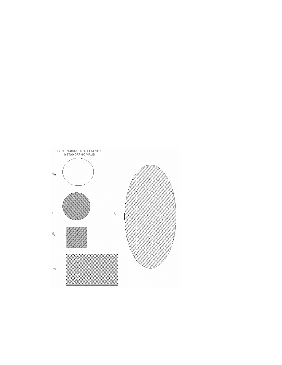
not decrypt to a constant virus body. A metamorphic virus changes its “shape” but not its
behavior. This is illustrated diagrammatically by Szor in [20], and is shown in Figure 1.
Figure 1 Multiple shapes of a metamorphic virus body [20].
5
Different techniques have been implemented by virus writers to create mutated virus
bodies. One of the simplest techniques employs register usage exchange; an example is
the W95/Regswap virus [19]. With this technique, a virus uses the same code but
different registers in a new generation. Such viruses can usually be detected by a
wildcard string [19].
A stronger technique employs permutation to reorder a virus’s subroutines, as seen in the
W32/Ghost virus [19]. With n different subroutines, a virus can generate n! different
virus generations. W32/Ghost has 10 subroutines and so it has 10! = 3,628,800 variations.
Even with the high number of subroutine combinations, the virus may still be detected
with search strings [19].
More complex metamorphic viruses insert garbage instructions between core
instructions. Garbage instructions are instructions that are either not executed or have no
effect on program outcomes [13]. An example of the former is the
nop instruction while
“
add eax, 0
” and “sub ebx, 0” are sample instructions that do not affect program results.
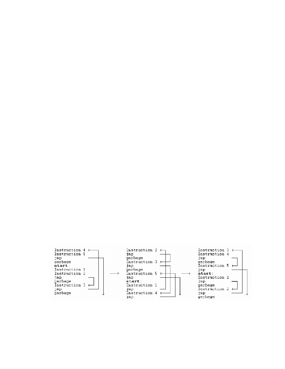
Alternatively, metamorphic viruses insert jump instructions into their code to point to the
next instruction of the virus code. The Win95/Zperm family of viruses creates new
mutations by removal and insertion of jump and garbage instructions as illustrated in
Figure 2 [19].
Figure 2 Zperm virus [19].

6
Another common metamorphic technique is substitution, which is the replacement of an
instruction or group of instructions with an equivalent instruction or group. For example,
a conditional jump (
Jcc) can be replaced by JNcc with inverted test condition and
swapped branch labels [24]. A “
push ebp; mov ebp, esp” sequence can be replaced by
“
push ebp; push esp; pop ebp” [19]. Sometimes, viruses implement instruction opcode
changes. For example, to zero out the register
eax, we can either xor its content with itself
or use
sub to achieve the same result. In other words, “xor eax, eax
” can be replaced by
“
sub eax, eax
” [19].
Transposition, or rearrangement of instruction order, is another technique used by
metamorphic viruses. Instruction reordering is possible if no dependency exists between
instructions. Consider the following example from [24]:
op1 [r1] [, r2]
op2 [r3] [, r4]
; here r1 and/or r3 are to be modified
Swapping of the two instructions is allowed if
1)
r1 not equal to r4; and
2)
r2 not equal to r3; and
3)
r1 not equal to r3.
Depending on the implemented techniques, a metamorphic virus can be very complex
and very hard to detect even with present day detection techniques. Unlike polymorphic
viruses, which decrypt themselves to a constant virus body in memory and provide a
complete snapshot of the decrypted virus body during its execution, metamorphic viruses
do not become constant anytime anywhere. The detection of metamorphic viruses has
been and will likely to continue to be an active research area.
2.1.4 Virus Construction Kits
Viruses are mostly written in assembly language, and not too many people can manage to
write complicated and functional assembly code. Some virus-writing groups try to make

7
the virus creation process quick and easy. They make available many virus construction
kits which can generate all kinds of malicious programs like viruses, worms, Trojan
horses and logic bombs. Virtually any type of virus can be created – DOS COM / EXE
viruses, 16-bit / 32-bit Windows viruses, script viruses, macro viruses, PE viruses, etc
[19]. These toolkits are designed to be simple to use and some even come with
commercial-grade interactive graphical interfaces. The tools allow anybody, novice or
expert, to generate malicious code quickly and easily.
User-friendly as they are, some of these tools are also built with very sophisticated
features such as anti-disassembly, anti-debugging, anti-emulation, and anti-behavior
blocking. Some kits come equipped with code morphing ability which allows them to
produce different-looking viruses. In this sense, the viruses they produce are
metamorphic, not just polymorphic. The more highly regarded ones among the 150+
generators available at the VX Heavens [22] include:
PS-MPC (Phalcon/Skism Mass-Produced Code generator)
G2 (Second Generation virus generator)
MPCGEN (Mass Code Generator)
NGVCK (Next Generation Virus Creation Kit)
VCL32 (Virus Creation Lab for Win32)
2.2 Antivirus Defense Techniques
As computer viruses evolve and become more complex, antivirus software must become
more sophisticated to defend against virus attacks. This section discusses the virus
detection techniques that have been deployed over the years. These techniques include:
1)
pattern-based scanning in first-generation scanners;
2)
nearly exact and exact identification in second-generation scanners;
3)
code emulation;
4)
heuristic analysis to detect new and unknown viruses [19].

8
2.2.1 First Generation Scanners
The simplest approach to virus detection is string scanning. First generation scanners
look for “virus signatures” which are sequences of bytes (strings) extracted from viruses
in files or in memory. A good signature for a virus consists of sequences of text strings or
byte codes found commonly in the virus but infrequently in benign programs. Usually, a
human expert converts the virus binary code into assembly code, looks for sections that
signify viral activities and picks the corresponding bytes in the machine code to be the
virus signature. More efficient methods use statistical techniques to extract good
signatures automatically [8].
Virus signatures are organized into databases. To identify virus infection, virus scanners
check specific areas in files or system areas and match them against known signatures in
databases. Some simple scanners also support wildcard search strings, such as “
??02 33C9
8BD1 419C” where the wildcard is indicated by ‘?
’. Wildcard strings allow skipped bytes
and regular expressions and can sometimes be used to detect encrypted or even
polymorphic viruses [19]. Using a search string from the common code areas of all
known variants of a virus to scan for the virus family is known as generic detection [19].
A generic string typically contains wildcards.
To speed up detection, some scanners search only the start and the end of a file instead of
the entire file as early computer viruses are mostly prepending (i.e., attached to the front
of the host programs) or appending (i.e., attached to the end of the hosts). Faster scanners
look for entry-points, which are common targets of computer viruses, in the headers of
executable files.
2.2.2 Second Generation Scanners
Second-generation scanners refine the detection process to detect viruses that evolve to
mutate their body. Smart scanning ignores junk instructions like
nop and excludes them in
virus signatures. Nearly exact identification uses double strings, cryptographic

9
checksums, or hash functions to achieve higher speed and greater accuracy. Exact
identification uses all (as opposed to one in nearly exact identification) constant ranges of
the virus bytes to calculate a checksum. Exact identification scanners are usually slower
than simple scanners but a well-written one can differentiate virus variants precisely.
2.2.3 Code Emulation
With code emulation, anti-virus software implements a virtual machine to simulate CPU
and memory activities. Scanners execute the virus code on the virtual machine rather than
on the real processor. Depending on how well the virtual machine mimics system
functionalities, few viruses are able to recognize that they are confined and examined in a
virtual environment.
Code emulation is a very powerful technique, particularly in dealing with encrypted and
polymorphic viruses. Encrypted and polymorphic viruses decrypt themselves in memory.
If an emulator is run long enough, the decrypted virus body will eventually present itself
to a scanner for detection. The scanner can check its virtual machine’s memory when a
maximum number of iterations or other stop conditions are met. Alternatively, string
scanning can be done periodically every predefined number of iterations. In this way,
complete decryption of the virus body is not necessary as long as the decrypted part is
long enough for identification. Code emulation can also be applied to metamorphic
viruses that use single or multiple encryptions.
Code emulation can become too slow to be useful if the decryption loop is very long,
particularly when a virus inserts garbage instructions in its polymorphic decryptor. A new
decryption technique uses code optimization to reduce the polymorphic decryptor to its
core instruction set. As the emulator iterates through the decryption loop, it removes junk
and other instructions that do not change program state. Code optimization speeds up
emulation and provides a profile of the decryptor for detection [19].

10
2.2.4 Heuristic Analysis
Heuristic analysis is used to detect new or unknown viruses. Often times, it is used to
detect variants of an existing virus family. Heuristic methods can be static or dynamic.
Static heuristics base the analysis on file format and the code structure of virus fragments.
Dynamic heuristics use code emulation to simulate the processor and operating system
and detect suspicious operations while the virus code is executed on a virtual machine.
Heuristic analysis is prone to false positives. A false positive occurs when a heuristic
analyzer incorrectly tags a benign program as viral. These false alarms are not cost-
effective. Too many false positives destroy users’ trust and make a system more
vulnerable as users may mistakenly assume a false alarm when it is a real attack.
2.3 Use of Machine Learning Techniques
Various researchers have attempted to use machine learning techniques to perform
heuristic analysis on metamorphic viruses. This section covers the result and potential of
some of the techniques, which include:
1)
data mining methods
2)
neural networks
3)
hidden Markov models.
2.3.1 Data Mining Approach
Data mining methods are often used to detect patterns in a large set of data. These
patterns are then used to identify future instances in a similar type of data. Schultz et al.
experimented with a number of data mining techniques to identify new malicious binaries
[17]. They used three learning algorithms to train a set of classifiers on some publicly-
available malicious and benign executables. They compared their algorithms to a
traditional signature-based method and reported a higher detection rate for each of their
algorithms. However, their algorithms also resulted in higher false positive rates when
compared to signature-based method.

11
The key to any data mining framework is the extraction of features, which are properties
extracted from examples in the dataset. Schultz et al. extracted some static properties of
the binaries as features. These include system resource information (the list of DLLs, the
list of DLL function calls, and the number of different function calls within each DLL)
obtained from the program header, and consecutive printable characters found in the files.
The most informative feature they used was byte sequences, which were short sequences
of machine code instructions generated by the hexdump tool.
The features were used in three different training algorithms. There was an inductive
rule-based learner that generated Boolean rules to learn what a malicious executable was;
a probabilistic method that applied Bayes rule to compute the likelihood of a particular
program being malicious, given its set of features; and a multi-classifier system that
combined the output of other classifiers to give the most likely prediction.
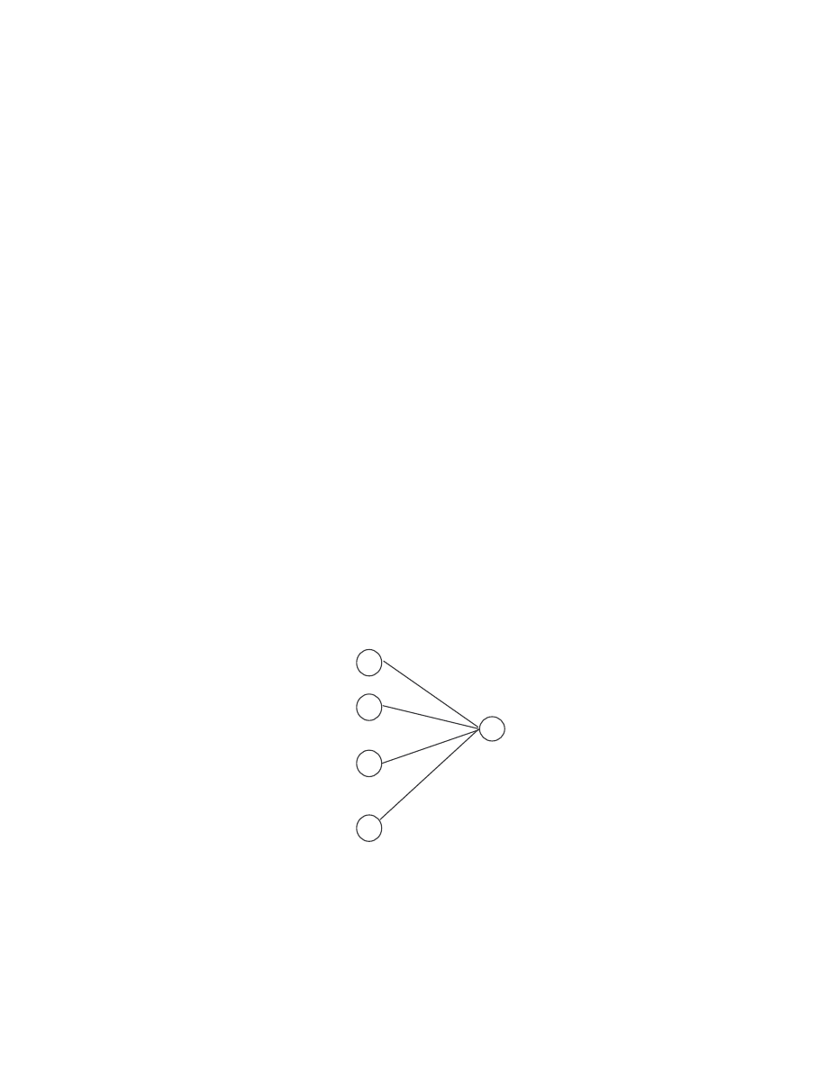
2.3.2 Neural Networks
Researchers at IBM implemented a neural network for heuristic detection of boot sector
viruses [21]. The features they used were short byte strings, called trigrams, which appear
frequently in viral boot sectors but not in clean boot sectors. They extracted about 50
features from a corpus of training data, which consisted of both viral and legitimate boot
sectors. Each sample in the dataset was then represented by a Boolean vector indicating
the presence or absence of these features.
The network was single-layered with no hidden units. It was trained using classic
backpropagation technique. One common problem with neural network is overfitting,
which occurs when a network is trained to identify the training set but fails to generalize
to unseen instances. To eliminate this problem, multiple networks were trained using
different features and a voting scheme was used to determine the final prediction.

12
The neural network was able to identify 80-85% of viral boot sectors in the validation set
with a false positive rate of less than 1%. The neural network classifier has been
incorporated into the IBM AntiVirus software which has identified about 75% of new
boot sector viruses since it was released [21]. A similar technique was later applied by
Arnold and Tesauro to successfully detect Win32 viruses [1]. From [21], we can
conclude that neural networks are very effective in detecting viruses closely related to
those in the training set. They can also identify new families of viruses containing similar
features as the training samples.
2.3.3 Hidden Markov Models
Hidden Markov models (HMMs) are well suited for statistical pattern analysis. Since
their initial application to speech recognition problems in the early 1970’s [15], HMMs
have been applied to many other areas including biological sequence analysis [10].
An HMM is a state machine where the transitions between states have fixed probabilities.
Each state in an HMM is associated with a probability distribution for observing a set of
observation symbols. We can “train” an HMM to represent a set of data, which is usually
in the form of observation sequences. The states in the trained HMM then represent the
features of the input data, while the transition and the observation probabilities represent
the statistical properties of these features. Given any observation sequence, we can match
it against a trained HMM to determine the probability of seeing such a sequence. The
probability will be high if the sequence is “similar” to the training sequences.
In protein modeling, HMMs are used to model a given family of proteins [11]. The states
correspond to the sequence of positions in space while the observations correspond to the
probability distribution of the 20 amino acids that can occur in each position. A model for
a protein family assigns high probabilities to sequences belonging to that family. A
trained HMM can then be used to discriminate family members from non-members.

13
Metamorphic viruses form families of viruses. Even though members in the same family
mutate and change their appearances, some similarities must exist for the variants to
maintain the same functionality. Detecting virus variants thus reduces to finding ways to
detect these similarities. Hidden Markov models provide a means to describe sequence
variations statistically. We propose to use HMMs similar to those used in protein
sequence analysis to model virus families. In virus modeling, the states correspond to the
features of the virus code, while the observations are instructions or opcodes making up
the program. A trained model should then be able to assign high probabilities to and thus
identify viruses belonging to the same family as the viruses in the training set.
3. SIMILARITIES BETWEEN VARIANTS OF METAMORPHIC VIRUSES
It has generally been agreed that for a virus to escape detection, metamorphism is the best
approach. Different generations of a virus must look different to avoid detection by
signature-based scanning. Some of the virus creation toolkits that we mentioned in
Section 2.1.4, including G2 (Second Generation virus generator) and NGVCK (Next
Generation Virus Creation Kit), come with the ability to generate morphed versions of
the same virus, even from identical configurations. In this section, we look at how
“effective” these generators are, or how “different” are the variants generated by the same
engine. We use a similarity index and also a graphical representation to display the
similarity between two assembly programs.
3.1 Method to Compare Two Pieces of Code
To compare two pieces of code, we employed the method developed by Mishra in [12].
His method compares two assembly programs and assigns a quantitative score to
represent the percentage of similarity between the two programs.
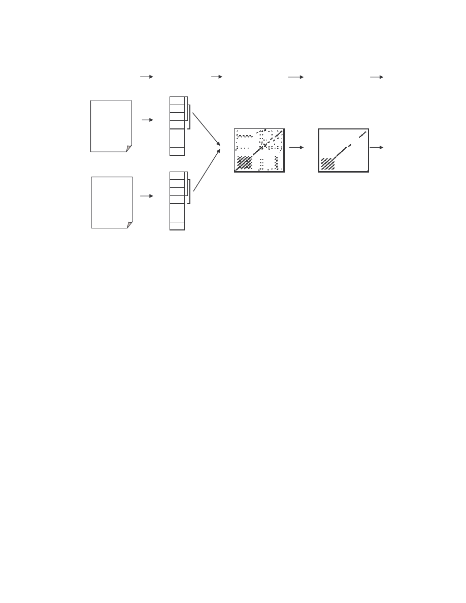
Mishra’s method is outlined below and is illustrated graphically in Figure 3.
1)
Given two assembly programs X, and Y for which we want to measure their
similarity, we extract the sequence of opcodes for each of the programs, excluding

14
comments, blank lines, labels, and other directives. The result is two opcode
sequences of length n, and m, where n and m are the numbers of opcodes in programs
X and Y, respectively. Each opcode is assigned an opcode number: the first opcode is
1, the second is 2, and so on.
2)
We compare the two opcode sequences by considering all subsequences of three
consecutive opcodes from each sequence. We count as a match any case where all
three opcodes are the same in any order, and we mark on a graph the coordinate (x, y)
of the match where x is the opcode number of the first opcode of the three-opcode
subsequence in program X and y is the opcode number of the opcode subsequence in
program Y.
3)
After comparing the entire opcode sequences and marking all the match coordinates,
we obtain a graph plotted on a grid of dimension n × m. Opcode numbers of program
X are represented on the x-axis and those of program Y are represented on the y-axis.
To remove noise and random matches, we only retain those line segments of length
greater than the threshold value five.
4)
Since we are performing a sequential match between the two opcode sequences,
identical segments of opcodes will form line segments parallel to the main diagonal
(if n = m, the main diagonal is simply the 45 degree line). If a line segment falls right
on the diagonal, the matching opcodes are at identical locations on the two opcode
sequences. A line off the diagonal indicates that the matching opcodes appear at
different locations in the two files.
5)
For each axis, we count the number of opcodes that are covered by one or more of the
matching line segments. This number is divided by the respective total number of
opcodes (n for program X and m for program Y) to give the percentage of opcodes
that match some opcodes in the other program. The similarity score for the two
programs is the average of these two percentages.
15
Opcode sequences
Score
0
call
1
pop
2
mov
3
sub
…
m-1
m-1
…
score =
n-1 jmp
average
% match
0 push
0
n-1
0
n-1
1
mov
2
sub
3
and
…
…
m-1 retn
Program X
Graph of real matches
P
ro
gr
am
Y
P
ro
gr
am
Y
(lines with length > 5)
(matching 3 opcodes)
Assembly programs
Program X
Graph of matches
Program X
Program Y
Figure 3 Process of finding the similarity between two assembly programs.
3.2 Test Data
We analyzed 45 viruses generated by four virus generators that we downloaded from VX
Heavens [22]. We also compared some randomly chosen utility programs from the
Cygwin DLL [4] to see how viruses differ from “normal” executable files. The programs
that we analyzed include:
20 viruses generated by NGVCK (Next Generation Virus Creation Kit) version
0.30 released in June 2001;
10 viruses generated by G2 (Second Generation virus generator) version 0.70a
released in January 1993;
10 viruses generated by VCL32 (Virus Creation Lab for Win32) released in
February 2004;
5 viruses generated by MPCGEN (Mass Code Generator) version 1.0 released in
1993;
20 randomly chosen utility executables from the Cygwin DLL version 1.5.19
.
16
The virus variants were named after their generators as follows:
the 20 viruses generated by NGVCK were named NGVCK0 to NGVCK19;
the 10 generated by G2 were named G0 to G9;
the 10 generated by VCL32 were named VCL0 to VCL9;
the 5 generated by MPCGEN were named MPC0 to MPC4
.
The 20 random utilities files were named R0 to R19.
The viruses created by the virus generators were in assembly source code. To make virus
executable files, we assembled them with the Borland Turbo Assembler TASM 5.0. The
generated executables were then disassembled by the IDA Pro Disassembler [6] version
4.6.0. All the disassembling used the same default settings. The cygwin utilities were also
disassembled by IDA Pro. The sequence of process is summarized as:
TASM, TLINK
IDA Pro
Virus Assembly Source
Virus Executables
Disassembled Virus ASM Files
Random Cygwin Executables
Diassembled Random ASM Files
We added the prefix “IDA_” to the respective file names to denote that the files were
disassembled ASM files created by IDA Pro and to distinguish them from the original
ASM files. For example, the file disassembled from R0.EXE was named IDA_R0.ASM.
We compared the disassembled assembly (ASM) files instead of the original assembly
codes generated by the virus generators. We believed by assembling and disassembling
with the same tools using the same settings, we can eliminate some differences due to
different coding style of the different virus writers. The standardized disassembling
process makes for more accurate comparison when we compare the viruses generated by
different generators, or when we compare viruses with random “normal” programs. It
makes the similarity measure better reflect the effectiveness of the metamorphism
employed. The process also simulates a more realistic scenario because when detecting
viruses in real environment, what we have available are virus executables. That is,
17
disassembling and analyzing the resultant assembly files is what we need to do in
practice.
3.3 Test Results
For each of the virus generator, we compared each of the viruses to all the other viruses
generated by the same generator, to see how “effective” the generator is in terms of
generating different-looking virus variants. For each pair of virus variants under
comparison, we computed their similarity score using the method described above in
Section 3.1. Comparisons were also made between the random normal files. The raw
similarity scores of all the comparisons are given in Table A-1 to Table A-5 in Appendix
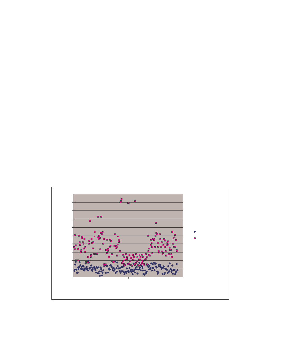
A. Figure 4 below is a scatter plot showing the similarity scores of the 190 pair-wise
comparisons among the 20 NGVCK viruses and the 190 pair-wise comparisons among
the 20 normal files. Clearly, similarities between NGVCK virus variants are lower than
those between normal files.
0.0
0.1
0.2
0.3
0.4
0.5
0.6
0.7
0.8
0.9
1.0
0
50
100
150
200
Comparison number
S
im
ila
ri
ty
s
co
re
NGVCK viruses
Normal files
Figure 4 Scatter plot showing similarity scores between NGVCK virus variants and between normal
files.
18
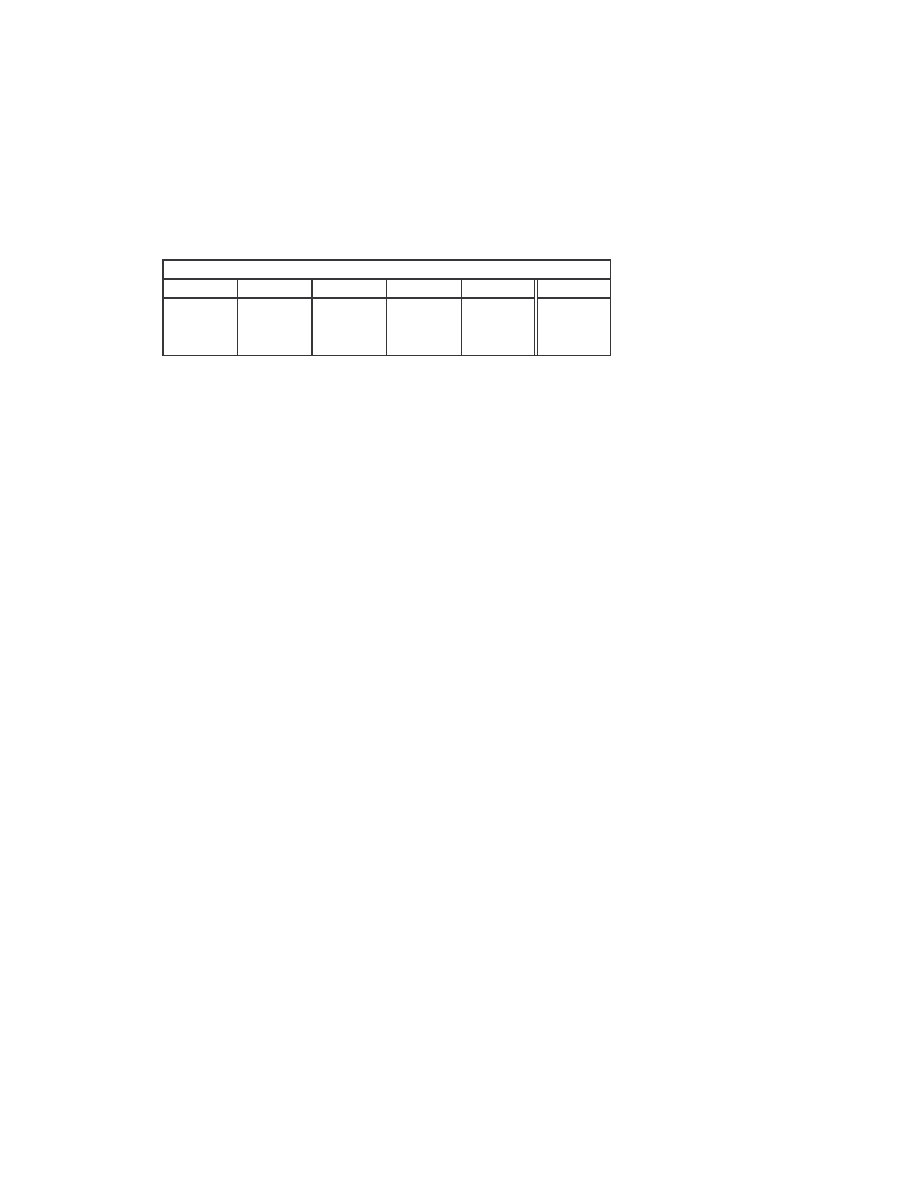
The minimum, maximum, and average scores of each generator and the normal files are
summarized below in Table 1.
NGVCK
G2
VCL32
MPCGEN Normal
min
0.01493
0.62845
0.34376
0.44964
0.13603
max
0.21018
0.84864
0.92907
0.96568
0.93395
average
0.10087
0.74491
0.60631
0.62704
0.34689
Minimum, maximum, and average similarity scores
Table 1 Minimum, maximum, and average similarity scores between virus variants generated by the
generators and between normal files.
Comparing the four generators, NGVCK generates viruses of the lowest similarities,
which range from 1.5% to 21.0% with an average of about 10.0%. The other generators
are not as effective at generating different-looking viruses. The similarities between two
variants of the same virus range from 34.4% to 96.6%, and the average scores of G2,
VCL32, and MPCGEN are 74.5%, 60.6%, and 62.7%, respectively. Compare to random
normal files, which have an average similarity of 34.7%, we can see that the viruses that
NGVCK generates are substantially different from one another, while the virus variants
generated by the other generators are more similar to one another than normal files.
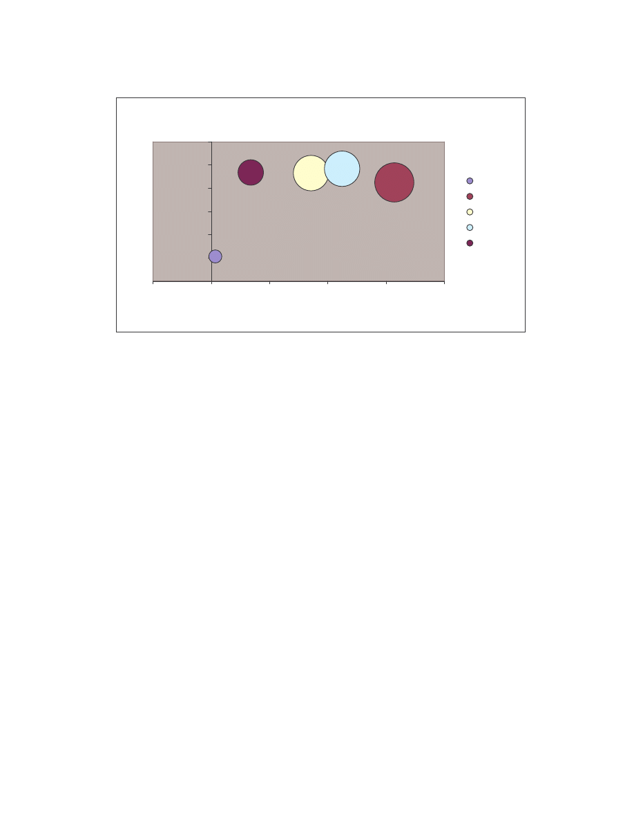
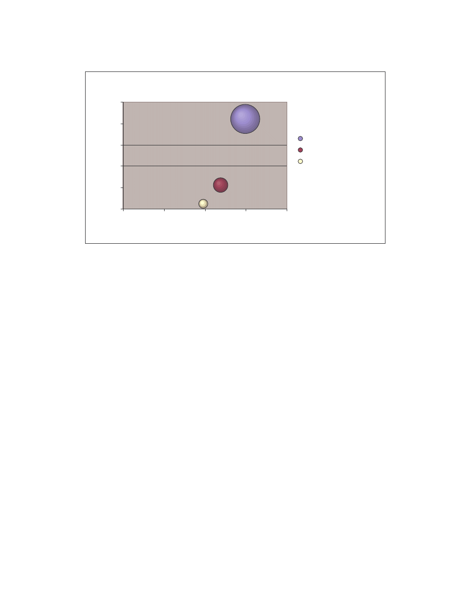
These comparison results are represented graphically by the bubble graph in Figure 5.
Here the minimum score is shown along the x-axis; the maximum score is shown along
the y-axis; and the size of the bubble represents the average similarity. Under this
representation, an effective generator would have a bubble that is very close to the origin
and also has a very small size, since effectively morphed variants of a virus should have
low minimum, low maximum and low average similarities.
19
Size of bubble = average similarity
NGVCK
G2
VCL32 MPCGEN
Normal
0
0.2
0.4
0.6
0.8
1
1.2
-0.2
0
0.2
0.4
0.6
0.8
Minmum similarity score
M
ax
im
um
s
im
ila
ri
ty
s
co
re
NGVCK
G2
VCL32
MPCGEN
Normal
Figure 5 Bubble graph showing minimum, maximum, and average similarity between virus variants
generated by each generator and between normal files.
As is shown in the graph, NGVCK clearly outperforms the other generators in terms of
generating different-looking viruses. VCL32 and MPCGEN have similar morphing
ability as their variants have comparable minimum, maximum, and average similarities.
G2 viruses have a higher average similarity, as is represented by the bigger bubble size,
although the maximum similarity of the variants is lower than that of VCL32 and
MPCGEN viruses. Normal files have similarities higher than NGVCK viruses but lower
than virus variants produced by generators G2, VCL32, and MPCGEN.
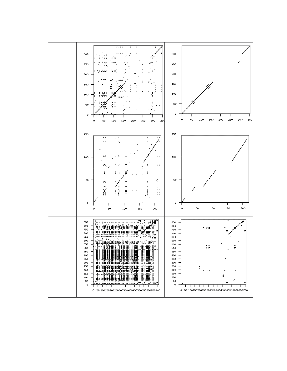
The following table shows the similarity graphs of some of the virus pairs. For each
generator, we chose a representative pair which has a similarity score close to the average
similarity score, to illustrate how a typical virus pair differ from each other. The first
column gives the virus names with their similarity score in parenthesis. The second
column shows the graphs of all matches, as defined in Section 3.1 above. The third
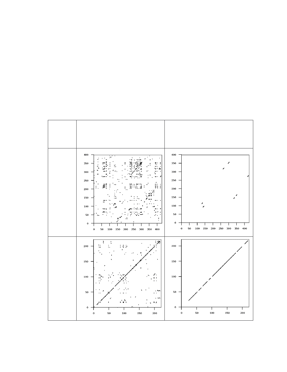
20
column shows the graphs of real matches after noise and random matches have been
removed. The pairs selected and their scores are:
IDA_NGVCK0 against IDA_NGVCK8, similarity = 11.9%
IDA_G4 against IDA_G7, similarity = 75.2%
IDA_VCL0 against IDA_VCL9, similarity = 60.2%
IDA_MPC1 against IDA_MPC3, similarity = 58.0%
normal files IDA_R0 and IDA_R1, similarity = 35.7%.
Virus Pair
(Similarity
score)
Graph of all matches
(matching 3 consecutive opcodes in
any order)
Graph of real matches
(match of length > 5)
IDA_
NGVCK0-
IDA_
NGVCK8
(11.9%)
IDA_G4-
IDA_G7
(75.2%)
21
IDA_VCL
0-
IDA_VCL
9
(60.2%)
IDA_MPC
1-
IDA_MPC
3
(58.0%)
IDA_R0-
IDA_R1
(35.7%)
Table 2 Similarity graphs of four selected virus pairs and one normal file pair.
22
If we take a closer look at the graphs for the pair of G2 viruses and the pair of VCL32
viruses, we can see that the real matches are almost all along the diagonal. This indicates
that virus variants of the same virus have identical opcodes at identical positions. This is
obviously not very effective metamorphism. On the other hand, the matches between the
MPCGEN virus pair are off the diagonal, which shows that identical opcodes appear in
different positions of the two virus variants. From this evidence, we can say that
MPCGEN has a greater morphing ability than the other two generators. NGVCK is the
most effective in the sense that the match segments are very short and that they are way
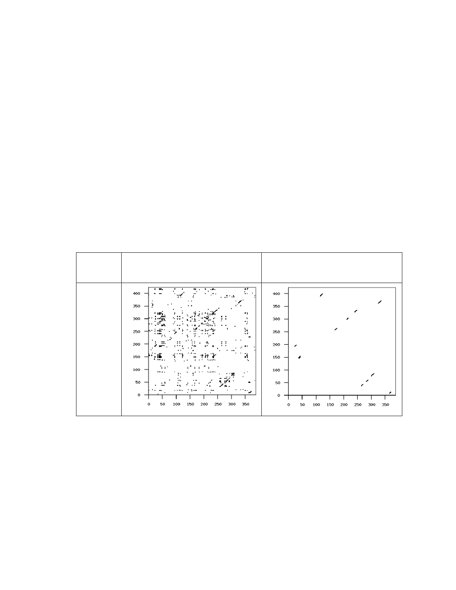
off the diagonal. Even if we look at the pair that has the highest similarity
(IDA_NGVCK7 and IDA_NGVCK14, similarity = 21.0%), the match segments are still
short and off the diagonal. The two similarity graphs of this pair are shown below.
Virus Pair
(score)
Graph of all matches
Graph of matches of length > 5
IDA_
NGVCK7-
IDA_
NGVCK14
(21.0%)
Table 3 Similarity graphs of the NGVCK virus pair that has the highest similarity.
As the Next Generation Virus Creation Kit (NGVCK) was found to be the most effective
based on our similarity measure, we were interested to know how the viruses it generates
differ from the viruses generated by the other generators. We compared the first 10
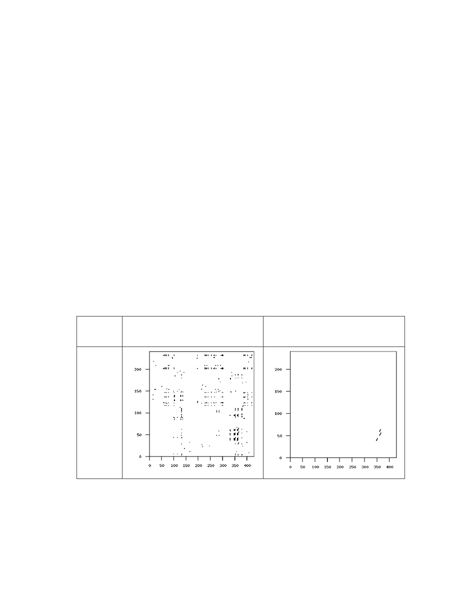
23
NGVCK viruses (IDA_NGVCK0 to IDA_NGVCK9) against each of the following
viruses:
IDA_G0 to IDA_G9 (10 files);
IDA_VCL0 to IDA_VCL9 (10 files);
IDA_MPC0 to IDA_MPC4 (5 files).
Our result shows that the NGVCK viruses are very different from the other viruses. Each
of the comparisons against the G2 viruses and against the MPCGEN viruses produces a
similarity score of 0. Of the 100 comparisons against the VCL32 viruses, 57 comparisons
have similarity score of 0, while the other 43 comparisons that show some similarity have
scores range from 1.2% to 5.5%, with an average of 2.4%. These scores are very low
compared to the similarity scores we have seen so far. The scores of the 43 pairs that
have similarity greater than zero are shown in Table A-6 in Appendix A. The similarity
graphs of the pair IDA_NGVCK0 and IDA_VCL4, which has the highest similarity score
of 5.5%, is shown in Table 4.
Virus Pair
(score)
Graph of all matches
Graph of matches of length > 5
IDA_
NGVCK0-
IDA_VCL4
(5.5%)
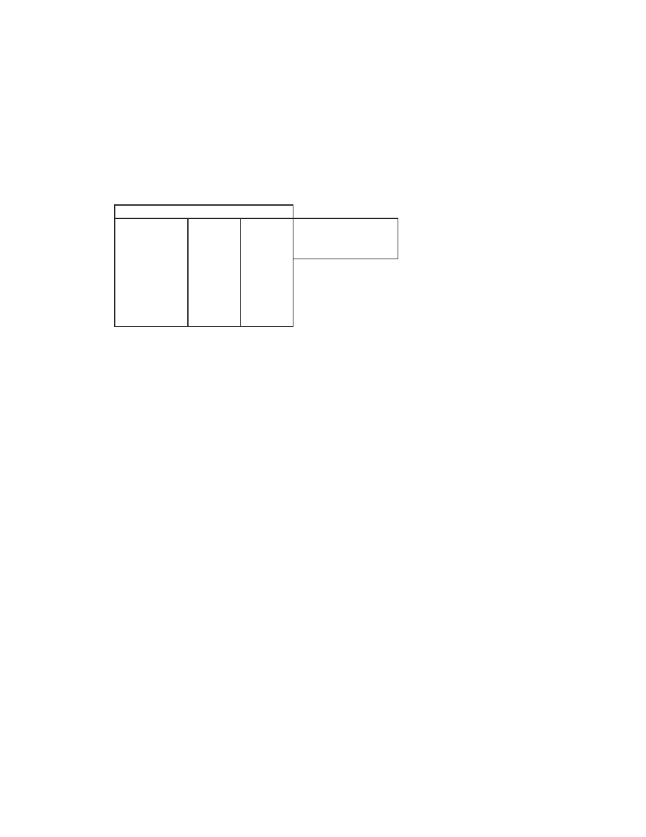
Table 4 Similarity graphs showing similarity between IDA_NGVCK0 and IDA_VCL4.
24
We also compared the NGVCK viruses to the normal files. All the 20 NGVCK viruses
were compared to the 20 normal files. All but 8 of the 400 comparisons again show no
similarity. The eight pairs that show some similarity have very low score of 0.98% to
1.12%. The scores are shown below in Table 5.
Similarity scores between files:
IDA_NGVCK2 IDA_R11
0.01001
min
0.00981
IDA_NGVCK5 IDA_R10
0.01123
max
0.01123
IDA_NGVCK6 IDA_R16
0.01021 average
0.01031
IDA_NGVCK7 IDA_R5
0.01007
IDA_NGVCK7 IDA_R6
0.00981
IDA_NGVCK7 IDA_R7
0.00990
IDA_NGVCK7 IDA_R8
0.01010
IDA_NGVCK7 IDA_R13
0.01115
Table 5 The eight pairs of NGVCK viruses and normal files that have non-zero similarity scores.
Using the same representation scheme, where we show the minimum similarity score
along the x-axis, the maximum score along the y-axis, and the average similarity by the
size of a bubble, we display the comparison results using the bubble graph in Figure 6.
The bubble labeled “NGVCK vs NGVCK” represents the result of comparing NGVCK
viruses against NGVCK viruses. The graph illustrates that NGVCK viruses not only have
low similarities among themselves, they show even lower similarities when compared to
other viruses or normal programs. We conclude that NGVCK viruses are very different
from other viruses and normal utility programs.
25
size of bubble = average similarity
NGVCK vs NGVCK
"NGVCK vs
VCL32"
NGVCK vs normal
0.00
0.05
0.10
0.15
0.20
0.25
0.000
0.005
0.010
0.015
0.020
Minimum similarity score
M
ax
im
u
m
s
im
ila
ri
ty
s
co
re
NGVCK vs NGVCK
"NGVCK vs VCL32"
NGVCK vs normal
Figure 6 Minimum, maximum, and average similarities between NGVCK virus variants, between
NGVCK viruses and VCL32 viruses, and between NGVCK viruses and normal files.
4. HIDDEN MARKOV MODELS TO DETECT VIRUSES IN SAME FAMILY
In this project, we developed a system to train multiple hidden Markov models (HMMs)
on a set of metamorphic virus variants. The trained models were tested for their ability to
detect morphed variants of the same virus. The effectiveness of the HMM approach is
determined by the detection rate, the number of false positives and false negatives, and
the overall accuracy.
4.1 Theory and Algorithms for Hidden Markov Models
A hidden Markov model is a statistical model that describes a series of observations
generated by a stochastic process, or Markov process. A Markov process is a sequence of
states, where the progression to the next state depends solely on the present state but not
on the past states. The Markov process in an HMM is “hidden”; what we can see is the
sequence of observations associated with the states. Our goal is to make use of the

26
observable information to gain insight into various aspects of the underlying Markov
process [18].
We illustrate these concepts by an example taken from [18]. Suppose we want to know
the average annual temperature of a particular location over a preceding period of several
consecutive years and suppose that there is no recording of past temperature of any form
for this location. Since there is no way to know the year-to-year temperature directly, we
look for evidence to predict the temperature indirectly.
For simplicity, we consider only two possible annual temperatures: “hot” (H) or “cold”
(C). Suppose we know that the probability of a hot year followed by another hot year is
0.7 and that of a cold year followed by another cold year is 0.6. This information can be
represented by the matrix:
6
.
0
4
.
0
3
.
0
7
.
0
C
H
C
H
.
Now assume research result tells us that the tree ring size of a certain kind of tree,
whether it is small (S), medium (M), or large (L), is related to the annual temperature as:
1
.
0
2
.
0
7
.
0
5
.
0
4
.
0
1
.
0
C
H
L
M
S
meaning that in a hot year, the probability of a tree having a small, medium, or a large
tree ring is 0.1, 0.4 and 0.5 respectively. If we observe the tree ring sizes for such a tree,
we can use this information to deduce the possible annual temperatures over the years of
interest.
In this example, the temperatures (H and C) are the states and the transition of
temperature from year to year defines the Markov process. Tree ring sizes (S, M, L) are
the observable outcomes and the probabilities of seeing the different tree ring sizes at

27
each temperature represent the probability distribution of the observation symbols at each
state. The actual states are “hidden” since we cannot directly observe the temperatures.
What we can see are the observations (tree ring sizes) and these are related to the states
statistically.
Suppose we represent the observation symbols S, M, L by 0, 1, 2 respectively and
suppose that a particular four-year series of observed tree ring sizes is given by the
observation sequence O = (0, 1, 0, 2). We might want to find the most likely state
sequence of the Markov process that generates the observation sequence. In other words,
we may want to determine the most likely annual temperatures (H or C) over this series
of four years from our observation of the tree ring sizes.
4.1.1 Notation
Let
T = the length of the observed sequence
N = the number of states in the model
M = the number of distinct observation symbols
O = the observation sequence = {O
0
, O
1
, …, O
T-1
}
Q = the set of states of the Markov process = {q
0
, q
1
, …, q
N-1
}
V = the set of observation symbols = {0, 1, … M – 1}
A = the state transition probability distributions
B = the observation probability distributions
π
= the initial state distribution
λ
= (A, B,
π
) = the HMM defined by its parameter A, B, and
π
.
Figure 7 shows a generic HMM. The state and observation at time t are represented by X
t
and O
t
respectively. The Markov process, which is hidden behind the dashed line, is
determined by the initial state X
0
and the A matrix. What we can observe are the
observations O
t
, which are related to the states of the Markov process by the B matrix.
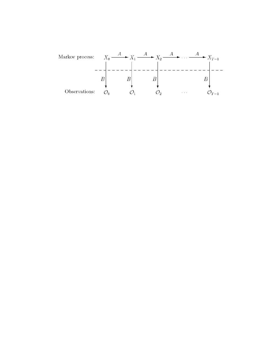
28
Figure 7 A generic hidden Markov model [18].
For our temperature example, the state transition matrix A is defined by the probabilities
of temperature transitions from year to year; the observation matrix B is defined by the
probabilities of observing the tree ring sizes. That is,
=
6
.
0
4
.
0
3
.
0
7
.
0
A
, and
=
1
.
0
2
.
0
7
.
0
5
.
0
4
.
0
1
.
0
B
which are the same matrices given previously.
The matrix A = {a
ij
} is N × N with
a
ij
= P(q
j
at t+1 | q
i
at t)
representing the probability of making a transition from state q
i
at time t to state q
j
at time
t+1.
The matrix B = {b
j
(k)} is N × M with
b
j
(k) = P(observation k at t | state q
j
at t)
representing the probability of observing symbol k at time t given we are in state q
j
at
time t.

29
The matrix
π
= {
π
i
} is 1 × M with
i
π
= P(q
i
at t = 0)
representing the probability of being initially in state q
i
at time 0. We assume for the
temperature example that
[
]
4
.
0
6
.
0
=
π
.
The matrices A, B, and
π
make up the parameters of an HMM. Note that A, B,
π
are row
stochastic, i.e., each row of these matrices represents a probability distribution and
therefore must sum to 1 [18].
For a generic state sequence X = (x
0
, x
1
, x
2
, x
3
) of length four, with corresponding
observations O = (O
0
, O
1
, O
2
, O
3
). The probability of the state sequence X is given by
P(X |
λ
) =
π
x
0
b
x
0
(O
0
) a
x
0
, x
1
b
x
1
(O
1
) a
x
1
, x
2
b
x
2
(O
2
) a
x
2
, x
3
b
x
3
(O
3
)
where
π
x
0
is the probability of starting in state x
0
, b
x
0
(O
0
) is the probability of observing
O
0
at x
0
and a
x
0
, x
1
is the probability of transiting from state x
0
to state x
1
. This easily
generalizes to a sequence of any length.
In our temperature example, with observation sequence O = (0, 1, 0, 2), we can compute
the probability of this observation sequence having been generated by each four-state
sequence. For example, the probability that observation O was generated by the state
sequence HHCC is
P(HHCC) = 0.6(0.1)(0.7)(0.4)(0.3)(0.7)(0.6)(0.1) = 0.000212
In the same manner, we can compute the probability of each of the possible state
sequences of length four, given the fixed observation sequence O. These probabilities are
listed in Table 6. We will have some more to say about these probabilities when we
discuss the HMM algorithms.
30
state sequence
probability
HHHH
0.000412
HHHC
0.000035
HHCH
0.000706
HHCC
0.000212
HCHH
0.000050
HCHC
0.000004
HCCH
0.000302
HCCC
0.000091
CHHH
0.001098
CHHC
0.000094
CHCH
0.001882
CHCC
0.000564
CCHH
0.000470
CCHC
0.000040
CCCH
0.002822
CCCC
0.000847
probability
0.009629
max probability
0.002822
Table 6 Probabilities of observing O = (0, 1, 0, 2) for all possible 4-state sequences.
In general, the three problems that we are interested in solving with an HMM are [18]:
Given the model
λ
= (A, B,
π
) and an observation sequence O, find P(O |
λ
). That
is, find the likelihood of observing the sequence O given the model.
Given
λ
= (A, B,
π
) and an observation sequence O, find an optimal state
sequence that could have generated O. (This is what we wanted to do in the
temperature example above.) Note that “optimal” here has at least two
interpretations. We can reasonably define optimal as:
1)
the state sequence with the highest probability from among all possible state
sequences; or
2)
the state sequence that maximizes the expected number of correct states.
Given an observation sequence O, the number of states N, and the number of
symbols M, find the model parameters, i.e., the probabilities in the A, B, and
π
matrices, that maximize the probability of observing O. This is a discrete hill
climb on the (A, B,
π
)-parameter space. In other words, we re-adjust the model
parameters to best fit the observations
.

31
4.1.2 Algorithms
There exist efficient algorithms to solve the three problems listed above. A thorough
review of these algorithms can be found in [15] and [7]. In this section, we look at some
of these algorithms, which include:
the Forward-Backward algorithm for calculating the probability of being in a
state q
i
at time t given an observation sequence O;
the Viterbi algorithm for finding the most likely state sequence given O; and
the Baum-Welch algorithm for iteratively re-estimating the parameters A, B,
π
.
4.1.2.1
Finding the likelihood of an observation sequence: the Forward algorithm
In the previous section, we saw that the probability of an observation sequence O = (O
0
,
O
1
, …, O
T-1
) generated by a particular state sequence X = (x
0
, x
1
, …, x
T-1
) given a model
λ
is given by
)
(
...
)
(
)
(
)
|
,
(
1
,
,
1
,
0
1
1
2
2
1
1
1
0
0
0
−
−
−
−
=
T
x
x
x
x
x
x
x
x
x
x
O
b
a
a
O
b
a
O
b
X
O
P
T
T
T
π
λ
.
To find the probability of observing the sequence O, we generate all possible state
sequences X
i
of length T and sum over the probabilities P(O, X
i
|
λ
).
=
i
X
i
X
O
P
O
P
)
|
,
(
)
|
(
λ
λ
−
−
−
−
=
i
T
T
T
X
T
x
x
x
x
x
x
x
x
x
x
O
b
a
a
O
b
a
O
b
)
(
...
)
(
)
(
1
,
,
1
,
0
1
1
2
2
1
1
1
0
0
0
π
Going back to our temperature example, the probability of observing tree ring sizes O =
(0, 1, 0, 2) given our model is equal to the sum of all the probabilities listed in Table 6,
which is 0.009629.
The probability P(O |
λ
) tells us how well the observation sequence O matches the HMM
λ
. If
λ
has N states and O has length T, then there are N
T
possible state sequences.
32
Finding the probability P(O, X
i
|
λ
) for one of the state sequence X
i
requires about 2T
multiplications and so a direct computation of the summation requires about 2TN
T
computations, which is infeasible even for small HMMs.
Instead of generating all possible state sequences, we use the Forward algorithm
(sometimes called the -pass) to compute this probability efficiently. For t = 0, 1, …, T –
1 and i = 0, 1, …, N – 1, define a forward variable
)
|
,...,
,
(
)
(
,
1
0
λ
α
i
t
t
t
q
x
O
O
O
P
i
=
=
which denotes the probability of observing the partial sequence (O
0
, O
1
, …, O
t
) up to
time t and being in state q
i
at time t. The forward variables can be found recursively using
the following recurrence relation:
Step 1 Initialization:
0
(i) =
π
i
b
i
(O
0
), for i = 0, 1, …, N – 1
Step 2 Induction:
)
(
)
(
)
(
1
0
1
t
i
N
j
ji
t
t
O
b
a
j
i
=
−
=
−
α
α
,
for t = 1, 2, …, T – 1 and i = 0, 1, …, N – 1.
Figure 8 illustrates the inductive process of finding
t
(i) using the variables
t-1
(j).
q
0
a
0i
q
1
a
1i
q
i
q
j
a
ji
b
i
(O
t
)
a
N- 1i
q
N-1
t - 1
t
t- 1
(j )
t
(i )
…
…
Figure 8 Inductive process of finding
t
(i) from variables
t-1
(j).

33
The probability of observing the sequence O given the model
λ
, P(O |
λ
), can then be
calculated as
−
=
=
=
1
0
,
1
0
)
|
,...,
,
(
)
|
(
N
i
i
T
T
q
x
O
O
O
P
O
P
λ
λ
−
=
−
=
1
0
1
)
(
N
i
T
i
α
.
The recursive computation requires N
2
T multiplications, which is much better than 2TN
T
for the naive approach.
4.1.2.2
Finding the most likely state sequence: the Viterbi algorithm
Given an observation sequence O = (O
0
, O
1
, …, O
T-1
) and an HMM
λ
, the Viterbi
algorithm finds a highest scoring overall path X* that maximizes the probability P(O, X |
λ
). We can determine the state sequence that is mostly likely to occur given the
observation sequence.
For t = 0, 1, …, T – 1 and i = 0, 1, …, N – 1, let
t
(i) denote the probability of the most
probable state path (x
0
, x
1
, …, x
t
) that generates the partial sequence (O
0
, O
1
, …, O
t
) up to
time t and ending in state q
i
,
)
|
,
,...,
,
,
,...,
,
(
max
)
(
1
1
0
,
1
0
...
1
0
λ
δ
i
t
t
t
x
x
t
q
x
x
x
x
O
O
O
P
i
t
=
=
−
−
The
t
(i) values can be found recursively as follows:
Step 1 Initialization:
0
(i) =
π
i
b
i
(O
0
),
for i = 0, 1, …, N – 1
Step 2 Induction:
)
(
]
)
(
[
max
)
(
1
1
0
t
i
ji
t
N
j
t
O
b
a
j
i
−
−
≤
≤
=
δ
δ
, for t = 1, 2, …, T – 1 and i = 0, 1, …, N – 1.

34
At each successive t, the algorithm gives the probability of the best path ending at each of
the states i = 0, 1, …, N – 1. Consequently, the probability of the most likely state
sequence for the observation sequence O is
[
]
)
(
max
*
1
1
0
i
P
T
N
i
−
−
≤
≤
=
δ
The Viterbi algorithm is similar to the Forward algorithm, except that maximizations
replace the summations in the recursive calculations. Notice that the
t
(i) values are
probabilities values only. To actually find the state sequence X*, we can use back-
pointers at each step to keep track of the best states chosen along the path. The path can
then be extracted by backtracking from the highest-scoring final state.
For our temperature example given at the beginning of Section 4.1, the mostly likely state
sequence is CCCH, having the highest probability of 0.002822 as shown in Table 6.
4.1.2.3
Finding the optimal model parameters: the Baum-Welch algorithm
One of the most useful features of an HMM is that we can efficiently re-adjust the model
parameters to best fit the observations. Given the matrix dimensions N and M, we can
iteratively re-estimate the elements of A, B, and
π
so that the probability of observing an
observation sequence O is maximized.
Before we discuss the re-estimation algorithm, let us first take a look at the Backward
algorithm, or -pass, which is analogous to the -pass given above. For t = 0, 1, …, T – 1
and i = 0, 1, …, N – 1, define the backward variable
)
,
|
,...,
,
(
)
(
1
2
1
λ
β
i
t
T
t
t
t
q
x
O
O
O
P
i
=
=
−
+
+
which denotes the probability of observing the partial sequence (O
t+1
, O
t+2
, …, O
T-1
)
given we are in state q
i
at time t.
t
(i) measures the probability after time t and can be obtained recursively starting at the
end of the sequence:
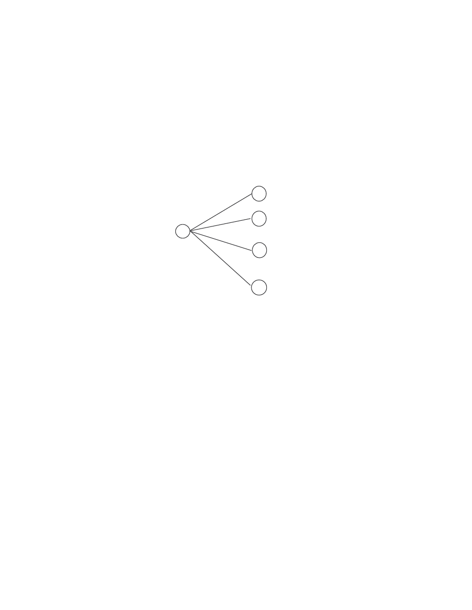
35
Step 1 Initialization:
T-1
(i) = 1, for i = 0, 1, …, N – 1
Step 2 Induction:
−
=
+
+
=
1
0
1
1
)
(
)
(
)
(
N
j
t
t
j
ij
t
j
O
b
a
i
β
β
, for t = T – 2, T – 1, …, 0 and i = 0, 1, …, N – 1.
Figure 9 illustrates the recursive process.
q
0
b
0
(O
t +1
)
a
i 0
q
1
b
1
(O
t +1
)
q
i
a
i 1
a
ij
q
j
b
j
(O
t +1
)
a
iN- 1
q
N-1
b
N- 1
(O
t +1
)
t
t + 1
t
(i )
t+1
(j )
…
…
Figure 9 Inductive process of finding
t
(i) from variables
t+1
(j).
The Backward algorithm also gives us the probability of observing the sequence O given
the model
λ
, or P(O |
λ
), which should be the same number produced by the Forward
algorithm:
−
=
=
1
0
0
0
)
(
)
(
)
|
(
N
i
i
i
i
O
b
O
P
β
π
λ
.
Now, define the probability of being in state q
i
at time t given the observation sequence O
and the model
λ
, for t = 0, 1, …, T – 2 and i = 0, 1, …, N – 1, as
)
,
|
(
)
(
λ
γ
O
q
x
P
i
i
t
t
=
=
.

36
This probability can be obtained from the forward-backward variables as
)
|
(
)
(
)
(
)
(
λ
β
α
γ
O
P
i
i
i
t
t
t
=
−
=
=
1
0
)
(
)
(
)
(
)
(
N
i
t
t
t
t
i
i
i
i
β
α
β
α
since
t
(i) accounts for the observations up to time t and
t
(i) accounts for the
observations after time t given we are in state q
i
at time t. The denominator P(O |
λ
) =
−
=
1
0
)
(
)
(
N
i
t
t
i
i
β
α
is the normalization factor, which makes
t
(i) a probability distribution
and sum to 1.
Next, define the joint probability of being in state q
i
at time t and transiting to state q
j
at
time t + 1, for t = 0, 1, …, T – 2 and i, j
}
1
,...,
1
,
0
{
−
∈
N
, as
)
,
|
,
(
)
,
(
1
λ
γ
O
q
x
q
x
P
j
i
j
t
i
t
t
=
=
=
+
.
This probability can be written in terms of , , A, and B as
)
|
(
)
(
)
(
)
(
)
,
(
1
1
λ
β
α
γ
O
P
j
O
b
a
i
j
i
t
t
j
ij
t
t
+
+
=
.
The relationship among these probabilities is illustrated graphically in Figure 10.
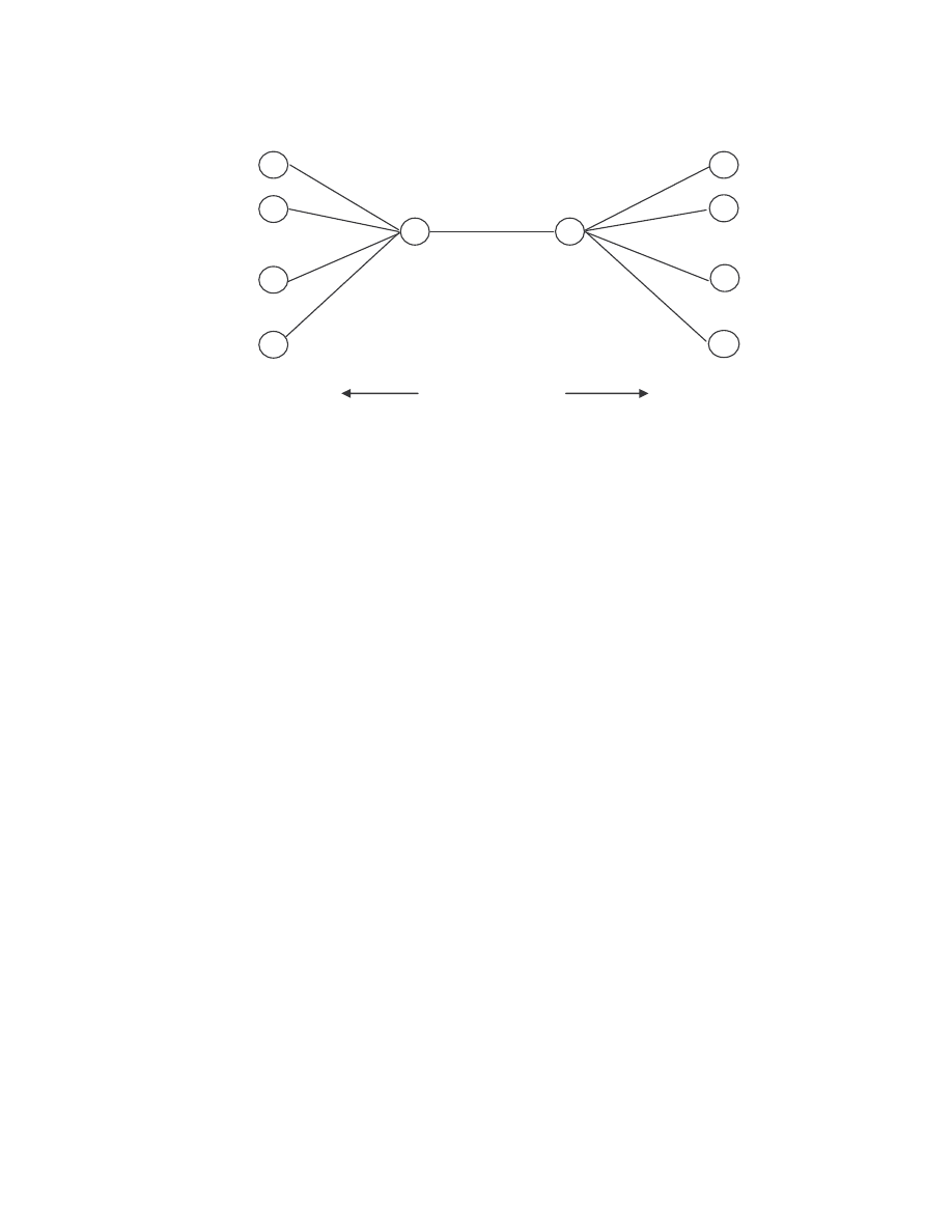
37
q
i
q
j
a
ij
b
j
(O
t +1
)
t - 1
t
t + 1
t + 2
t+1
(j )
t
(i )
…
…
…
…
Figure 10 Variables for the computation of the joint probability
t
(i, j).
The
t
(i) and
t
(i, j) are related by
−
=
=
1
0
)
,
(
)
(
N
j
t
t
j
i
i
γ
γ
t
(i) gives us the probability of being in state q
i
at time t. If we sum the probability over
all possible T, we get the expected number of transitions from state q
i
to any state.
t
(i, j)
gives us the joint probability of being in state q
i
at time t and in state q
j
at time t + 1. The
summation of
t
(i, j) over T thus gives the expected number of transitions from state q
i
to
state q
j
. In other words,
−
=
2
0
)
(
T
t
t
i
γ
= the expected number of transitions from state q
i
to any state, and
−
=
2
0
)
,
(
T
t
t
j
i
γ
= the expected number of transitions from state q
i
to state q
j
.

38
We can now re-estimate the parameters of
λ
= (A, B,
π
) using the following formulae:
For i = 0, 1, …, N – 1,
)
(
0
i
i
γ
π
=
= probability of being in state q
i
at t = 0.
For i = 0, 1, …, N – 1 and j = 0, 1, …, N – 1,
−
=
−
=
=
2
0
2
0
)
(
)
,
(
T
t
t
T
t
t
ij
i
j
i
a
γ
γ
i
j
i
q
q
q
of
out
ns
transitio
of
number
Expected
to
from
ns
transitio
of
number
Expected
=
For j = 0, 1, …, N – 1 and k = 0, 1, …, M – 1,
−
=
−
=
=
=
2
0
2
0
)
(
)
(
)
(
T
t
t
T
k
O
t
t
j
j
j
k
b
t
γ
γ
j
j
q
k
q
state
in
is
model
the
times
of
number
Expected
n
observatio
with
state
in
is
model
the
times
of
number
Expected
=
We re-estimate
λ
iteratively until P(O |
λ
) does not increase (or the increase is less than a
predefined threshold) or until the maximum number of iterations is reached. The
complete Baum-Welch expectation-maximization (EM) algorithm can be summarized as:
1)
Initialize
λ
= (A, B,
π
) with a best guess. If no prior information is available, choose
random
π
i
1/N, a
ij
1/N, and b
j
(k) 1/M.
2)
Calculate
t
(i),
t
(i),
t
(i) and
t
(i, j).
3)
Re-estimate the model
)
,
,
(
π
λ
B
A
=
, and calculate P(O |
λ
).
4)
Stop if P(O |
λ
) – P(O |
λ
) is less than the predefined threshold or the maximum
number of iterations is reached; otherwise set
λ
=
λ
and goto (2).

39
4.1.2.4
Posterior state probabilities
The Viterbi algorithm given in Section 4.1.2.2 finds the most probable state path through
the model. But as we mentioned in Section 4.1.1, there is a second interpretation as to
what constitutes an “optimal” state sequence. Instead of finding the highest scoring
overall path, as is done by the Viterbi algorithm, we may want to find the most probable
state for each specific observation O
t
in the observation sequence O = (O
0
, O
1
, …, O
T-1
).
More generally, we may want to find the probability that observation O
t
is generated by
state q
i
given the sequence O, i.e., P(x
t
= q
i
| O,
λ
). This is called the posterior probability
of state q
i
at time t.
This posterior probability is exactly the
t
(i) variable defined above in Section 4.1.2.3,
which is given by
)
|
(
)
(
)
(
)
,
|
(
λ
β
α
λ
O
P
i
i
O
q
x
P
t
t
i
t
=
=
.
Hence, the optimal path that finds the most probable state for each position is obtained by
finding, for each t = 0, 1, …, T – 1, the state q
i
for which
t
(i) is maximum.
This state sequence is not necessarily the same as the highest scoring sequence found by
the Viterbi algorithm. We may be more interested in this sequence that maximizes all
posterior probabilities when there are many different paths that have probabilities very
close to the most probable one, or when we want to know only the state assignment at a
particular point t rather than the complete path. It is possible that this state sequence may
not be particularly likely as a path through the HMM. Sometimes it is not even a
legitimate path when some of the transitions between states are not allowed.
4.1.3 Implementation Issues: Underflow and Scaling
The HMM computations discussed in Section 4.1.2 require repeated multiplications of
the transition and observation probability values. One major challenge in the
implementation is to deal with these small products which tend to zero exponentially as T

40
increases and can easily cause underflow if care is not taken. To solve this problem, we
can scale the forward and backward variables while maintaining the validity of the re-
estimation formulae.
The scaled version of the Forward algorithm normalizes each
t
(i) by dividing by the sum
(over j) of all
t
(j) for each value t, or observation O
t
. Let
)
(
~ i
t
α
denotes the forward
probability that is scaled up to t – 1 but not scaled for t yet;
)
(
ˆ i
t
α
denotes the scaled
probability; and
)
(i
t
α
denotes the non-scaled probability as given in the original forward
algorithm. The scaling coefficient c
t
at each time t is defined by
−
=
=
1
0
)
(
~
1
N
j
t
t
j
c
α
,
where
−
=
=
1
0
0
0
)
(
1
N
j
j
c
α
and
)
(
)
(
ˆ
0
0
0
i
c
i
α
α
=
for i = 0, 1, …, N – 1 when t = 0.
Then for each t = 1, 2, …, T – 1, calculate
−
=
−
=
1
0
1
)
(
)
(
ˆ
)
(
~
N
j
t
i
ji
t
t
O
b
a
j
i
α
α
and
)
(
~
)
(
ˆ
i
c
i
t
t
t
α
α
=
for i = 0, 1, …, N – 1.
The scaled probabilities are now normalized so that
1
)
(
ˆ
1
0
=
−
=
N
i
t
i
α
. Also, it can be proven
by induction that
)
(
~
)
(
ˆ
i
c
i
t
t
t
α
α
=
)
(
...
1
0
i
c
c
c
t
t
α
=
.
Combining these two properties and setting t = T – 1, we have
−
=
−
=
1
0
1
)
(
ˆ
1
N
j
T
j
α

41
−
=
−
−
=
⇔
1
0
1
1
1
0
)
(
...
1
N
j
T
T
j
c
c
c
α
)
|
(
...
1
1
1
0
λ
O
P
c
c
c
T
−
=
⇔
∏
−
=
=
⇔
1
0
1
)
|
(
T
j
j
c
O
P
λ
.
To avoid underflow, we compute the log likelihood, log[P(O |
λ
)], instead of P(O |
λ
):
∏
−
=
=
1
0
1
log
)]
|
(
log[
T
j
j
c
O
P
λ
j
T
j
c
−
=
−
=
1
0
log
.
The same scale factor c
t
is used for
t
(i) so that
)
(
)
(
ˆ
i
c
i
t
t
t
β
β
=
. The computations of
t
(i)
and
t
(i, j) use the same formulae as given in Section 4.1.2.3 substituting
)
(
ˆ i
t
α
and
)
(
ˆ i
t
β
for
t
(i) and
t
(i). These values are then used to re-estimate the model parameters A, B,
and
π
.
The implementation of the Viterbi algorithm can also result in underflow. This is avoided
by taking logarithms. The underflow-resistant Viterbi algorithm is defined as:
Step 1 Initialization:
)]
(
log[
)
(
ˆ
0
0
O
b
i
i
i
π
δ
=
,
for i = 0, 1, …, N – 1
Step 2 Induction:
)]}
(
log[
]
log[
)
(
ˆ
{
max
)
(
ˆ
1
1
0
t
i
ji
t
N
j
t
O
b
a
j
i
+
+
=
−
−
≤
≤
δ
δ
,
for t = 1, 2, …, T – 1 and i = 0, 1, …, N – 1.

42
The optimal log probability is given by
)]
(
ˆ
[
max
*
log
1
1
0
i
P
T
N
i
−
−
≤
≤
=
δ
and as before back-pointers can be used to keep track of the optimal path.
4.2 HMM for Computer Virus Detection
Given a set of metamorphic virus variants, our goal is to train one or more hidden
Markov models (HMMs) to represent the statistical properties of the virus family so that
we can later use a trained model to determine whether a given program is similar to the
viruses in the training set.
We trained our models based on the assembly opcode sequences of the virus files. For
viruses originally generated in assembly source format, we first compiled the assembly
source into executables using TASM 5.0. We then disassembled the executables using
IDA Pro with identical default settings. We trained our models on the IDA-generated
files rather than the original assembly source from the virus generators. We believed this
makes our method more realistic. Disassembling executables is typically part of the virus
analysis process. This virus pre-processing procedure is the same as the one we used in
the virus similarity test in Section 3 and is summarized again below:
TASM, TLINK
IDA Pro
Virus Assembly Source
Virus Executables
Disassembled Virus ASM Files
There are generally two approaches to training an HMM when there are multiple
observation sequences. We can either concatenate the sequences and make them into one
long observation sequence; or train the HMM with each sequence separately and average
the parameters from the different trainings [7]. We chose the former approach in our
training process. With the set of pre-processed virus ASM files, we extracted the
assembly opcode sequences, concatenated them into one long sequence of opcodes and
used it to train our HMMs.

43
A trained model maximizes the probability of observing the training sequence. By
calculating the probability of observing any given sequence in the HMM and comparing
it to the probability of observing the training sequence, we know how well the given
sequence matches the training sequence, or how “similar” the given sequence is to the
training sequence. When trained with multiple sequences, the resulting HMM represents
the “average” behavior, or the behavior of all the sequences in the form of a statistical
profile. We can represent a whole virus family, as opposed to individual viruses, with a
single HMM. The probability of any sequence in the HMM then tells us how likely it is
that the given sequence belongs to the same virus family.
One extremely useful aspect of an HMM is that it tells us something about the training
sequence without any requirement that we interpret the observations or underlying
features. Without specific knowledge of the features of the metamorphic viruses, we
trained our HMMs using different number of states and examined the resulting
probabilities to deduce what features the states represent. The number of states N that we
tested were N = 2, 3, 4, 5, and 6. To remain flexible, we did not define a fixed set of
opcodes as observable symbols. Instead, we set M equal to the total number of distinct
opcodes actually seen in the training sequences for each model. The number of
observation symbols thus varied from model to model. With our data, M was typically
around 70 to 80. The viruses we trained on were about 350 to 450 opcodes long, with an
average length of 416 opcodes. Concatenating 160 virus opcodes to train a model made
the length of the observed training sequence T in the range of 66,000 to 67,000. The
average T for the models we trained was 66,650.
Our HMM implementation used the scaled version of the Forward and the Backward
algorithm as discussed in Section 4.1.3. To avoid underflow, we computed the log
likelihood, instead of the raw probability, of observing the training sequence in the model
at each step of the iterative training process. Re-estimation stopped when the log

44
likelihood of the training sequence converged or a maximum of 800 iterations had been
reached.
4.3 Training and Testing
We collected a large number of metamorphic virus variants generated by a virus creation
kit to form a data set. Training and testing was done using standard cross-validation
methodology [9]. With five-fold cross validation, we divide the data set into five equal-
sized subsets. Each time when we train a model, we choose one of the subsets as the test
set and train the model using data from the other four subsets. Because data from the test
set is not used during training, we can use it to evaluate the performance of the model
over unseen instances of the same virus. Repeating this process five times, choosing a
different subset as the test set each time, we can get five different models from the same
set of data.
Viruses generated by a code morphing generator form a virus family, as they are
morphed versions of the same virus and have the same behavior. We consider viruses
generated by different generators as belonging to different families. After training, an
HMM should assign high probabilities to files similar to the training viruses and low
probabilities to all other files, whether they are “normal” benign programs or viruses
from different families. We made a comparison set which consisted of normal
executables of sizes comparable to the executables of the viruses in the data set (about 8
KB). The comparison set also contained viruses created by generators other than the one
used to generate the data set.
With a trained model, we computed the log likelihood of the virus variants in the test set
and the programs in the comparison set. Log likelihood is strongly length dependent,
since it is a sum of log transition probabilities and log observation probabilities. A longer
sequence will naturally have more transitions and more observations and thus a greater
log likelihood, independent of how similar it is to the training sequences. Because the

45
sequences in the comparison set may have lengths different from the sequences in the
training and test set, we divided the log likelihood of a sequence by the sequence length
(which is the number of opcodes) to obtain the log likelihood per opcode (LLPO), which
adjusts for the length difference. This LLPO is the score of the sequence.
Comparing the scores of the files in the test set, which are viruses in the same family as
the files used for training, and the scores of the files in the comparison set, which are
random non-viral programs or viruses in other families, there should be a separation of
scores between the two sets as the trained model should assign higher probabilities and
thus higher LLPO to files in the same virus family. From these empirical scores, we
determined a threshold, above which we will consider a file as belonging to the same
family as the viruses in the training set. To classify whether a program is in the same
virus family as the training data, we compute its score and compare it to the threshold.
The training and classifying process is summarized below and is illustrated graphically in
Figure 11.
Training:
1)
Given a data set consisting of different variants of a metamorphic virus, pick one
subset as the test set and use the remaining four subsets for training.
2)
Train HMM
λ
for sequences in the training set until the log likelihood of the training
sequence converges or a maximum number of iterations is reached.
3)
Compute the score, i.e., the log likelihood per opcode (LLPO), of viruses in the test
set and other files in the comparison set.
4)
Determine a cutpoint (threshold) score above which a file is classified as a member
virus. The threshold separates virus family members from non-members.
5)
Repeat from (1), choosing a different subset as the test set, until all five subsets have
been chosen.
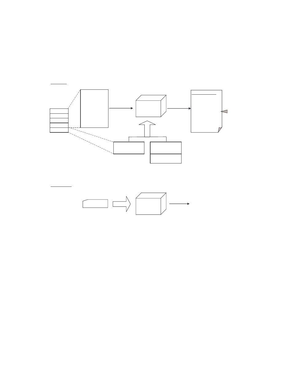
46
Classifying:
1)
To determine whether any program is part of the virus family, score and compare its
LLPO to the model thresholds.
Training:
(1)
Training set
(160 files)
(2) Training
(4)
Threshold
(3)
Data Set
(1)
Test set
Normal programs
(40 files)
(40 files)
Other viruses
(25 files)
Comparison Set
Classifying:
(3) Scoring
(1) Scoring
LLPO > Threshold ?
HMM
Scores (LLPO)
virus0 -2.0
virus1 -2.3
:
:
normal0 -11.3
:
other0 -8.9
HMM
Program A
Figure 11 Training and classifying process.
The HMM algorithms were implemented in C and compiled with Visual C++ 2005
Express Edition. We wrote some Ruby scripts using Ruby 1.8.4 on Windows [16] to
perform the cross-validation. All trainings are carried out on a Pentium M 1.4 GHz
machine running Windows XP Home Edition with 768 MB of RAM.
4.4 Data Used
Our data set consisted of 200 viruses generated by the Next Generation Virus Creation
Kit (NGVCK), which was shown to be the most effective of the four virus generators we

47
tested in Section 3. With five-fold cross validation, the number of viruses in each test set
was 40 and the number of sequences used for training was 160 for each model.
After training, we compared the scores of the 40 family viruses in the test set to the
scores of the programs in the comparison set. There were 65 files in the comparison set
consisting of both benign and viral programs. These included:
40 random executable files chosen from the Cygwin DLL (version 1.5.19) to
represent “normal” benign programs. The first 20 were the same ones that we
used in our similarity test in Section 3;
25 viruses generated by the three generators G2, MPCGEN, and VCL32. They
were the same programs that we tested for similarity in Section 3.
All these programs were unique and there were no duplicates. Training and testing used
files disassembled by IDA Pro (version 4.6.0) [6]. The four generators are downloadable
from [22] while the Cygwin DLL is available at [4].
The IDA-preprocessed files were named as follows:
the 200 viruses in the data set were named IDA_N0 to IDA_N199 (N for
NGVCK);
the 40 “normal” files in the comparison set were named IDA_R0 to IDA_R39 (R
for random);
the 25 “other” viruses in the comparison set were named IDA_V0 to IDA_V24 (V
for viruses
).
The 200 viruses in the data set were divided into five subsets according to virus number:
Test set 0: IDA_N0 to IDA_N39;
Test set 1: IDA_N40 to IDA_N79;
Test set 2: IDA_N80 to IDA_N119;
Test set 3: IDA_N120 to IDA_N159;
Test set 4: IDA_N160 to IDA_N199.

48
4.5 Experimental Results
For each N = 2, 3, 4, 5, and 6 hidden states, training and testing was run as described
above and five models were obtained for each N giving a total of 25 models.
4.5.1 Separation of Scores
We first examined how the HMMs separate viruses in the test set from normal benign
programs. We called viruses in the test set “family viruses” as they were generated by the
same virus generator (NGVCK) that created the viruses used for training. This is in
contrast with “non-family viruses” in the comparison set which were viruses generated by
generators other than NGVCK. The random utility files in the comparison set were called
“normal files”.
Of the 25 models, 23 models were able to make a clear separation of scores between
family viruses and normal files, meaning the scores (in log likelihood per opcode, LLPO)
of the 40 family viruses were always higher than the scores of the 40 normal files. Table
7 shows the scores of test set 0 using the model with N = 2 states. With this model, all
family viruses in the test set scored -4.43 or higher while all normal files scored -8.07 to
as low as -169.19. Figure 12 is a scatter plot showing all these scores. We can see that all
the normal file scores are below the family virus scores.
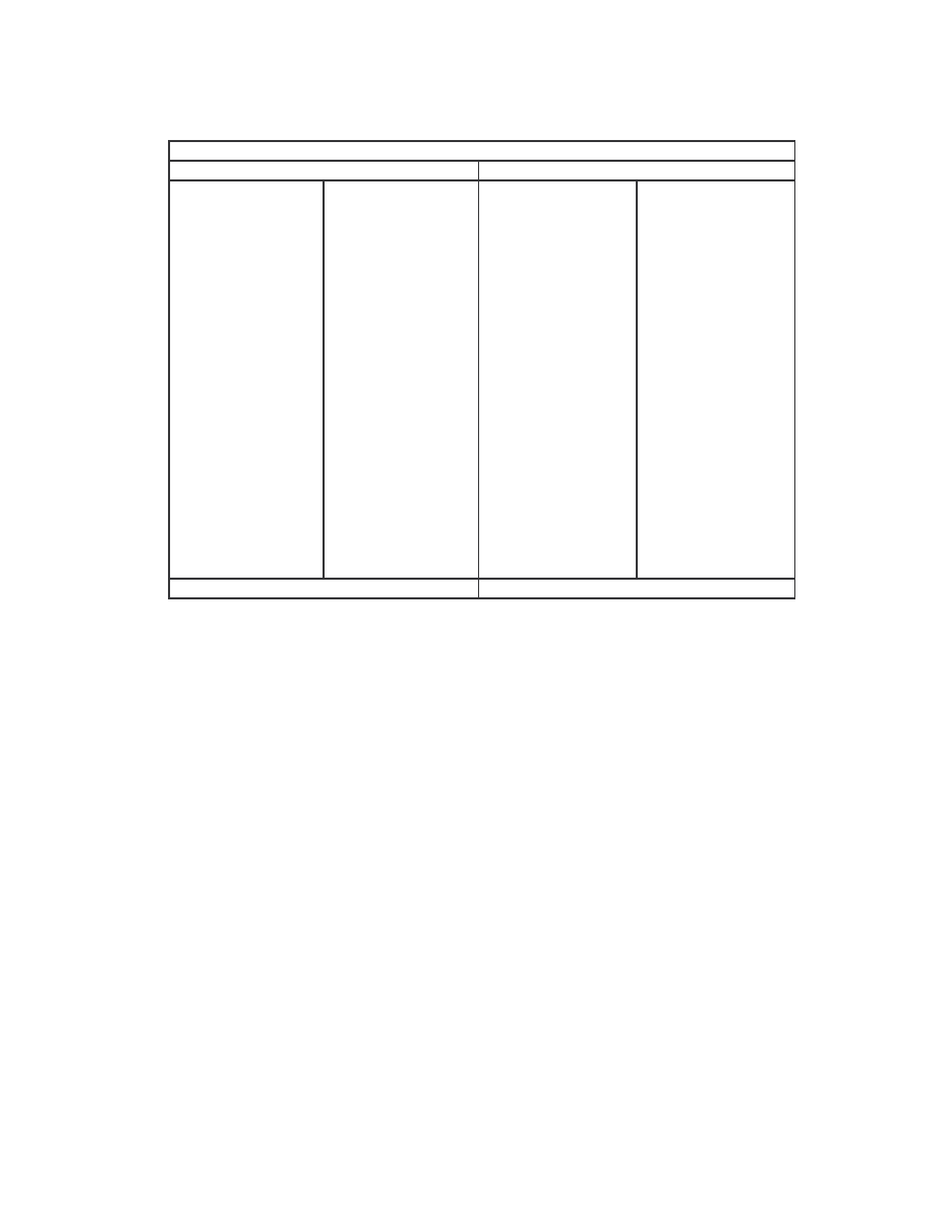
49
IDA_N0
-2.8384 IDA_N20
-2.8283 IDA_R0
-20.3522 IDA_R20
-33.1515
IDA_N1
-4.3805 IDA_N21
-2.7191 IDA_R1
-13.9877 IDA_R21
-14.2326
IDA_N2
-2.8561 IDA_N22
-2.8522 IDA_R2
-14.9357 IDA_R22
-12.9223
IDA_N3
-2.6847 IDA_N23
-2.7908 IDA_R3
-27.6756 IDA_R23
-16.9245
IDA_N4
-2.7891 IDA_N24
-2.7420 IDA_R4
-22.7756 IDA_R24
-30.9469
IDA_N5
-2.8767 IDA_N25
-2.8374 IDA_R5
-15.1323 IDA_R25
-9.1670
IDA_N6
-2.7910 IDA_N26
-2.7560 IDA_R6
-13.7367 IDA_R26
-22.6304
IDA_N7
-2.6920 IDA_N27
-2.7401 IDA_R7
-14.1954 IDA_R27
-21.8092
IDA_N8
-2.8229 IDA_N28
-2.7938 IDA_R8
-15.8122 IDA_R28
-14.3619
IDA_N9
-2.7144 IDA_N29
-2.8134 IDA_R9
-33.7738 IDA_R29
-22.0801
IDA_N10
-2.7786 IDA_N30
-2.9037 IDA_R10
-12.2689 IDA_R30
-19.1720
IDA_N11
-2.6820 IDA_N31
-4.4349 IDA_R11
-23.8743 IDA_R31
-22.5469
IDA_N12
-2.8562 IDA_N32
-2.7898 IDA_R12
-9.4898 IDA_R32
-31.5030
IDA_N13
-2.7386 IDA_N33
-2.7112 IDA_R13
-33.6615 IDA_R33 -149.0010
IDA_N14
-2.7785 IDA_N34
-4.4010 IDA_R14 -148.5225 IDA_R34
-42.8888
IDA_N15
-2.8147 IDA_N35
-2.8361 IDA_R15
-12.2724 IDA_R35
-51.2670
IDA_N16
-2.7484 IDA_N36
-2.8036 IDA_R16
-8.0663 IDA_R36
-21.4580
IDA_N17
-2.7643 IDA_N37
-2.8059 IDA_R17
-14.7949 IDA_R37
-17.9681
IDA_N18
-2.7781 IDA_N38
-2.9326 IDA_R18
-13.0679 IDA_R38 -169.1918
IDA_N19
-2.7906 IDA_N39
-2.7216 IDA_R19
-35.6981 IDA_R39
-45.4978
-8.0663
Normal files
Family viruses
Test set 0, N = 2
min LLPO
-4.4349
max LLPO
Table 7 LLPO scores of the 40 family viruses in test set 0 and the 40 normal files using the model
with N = 2.
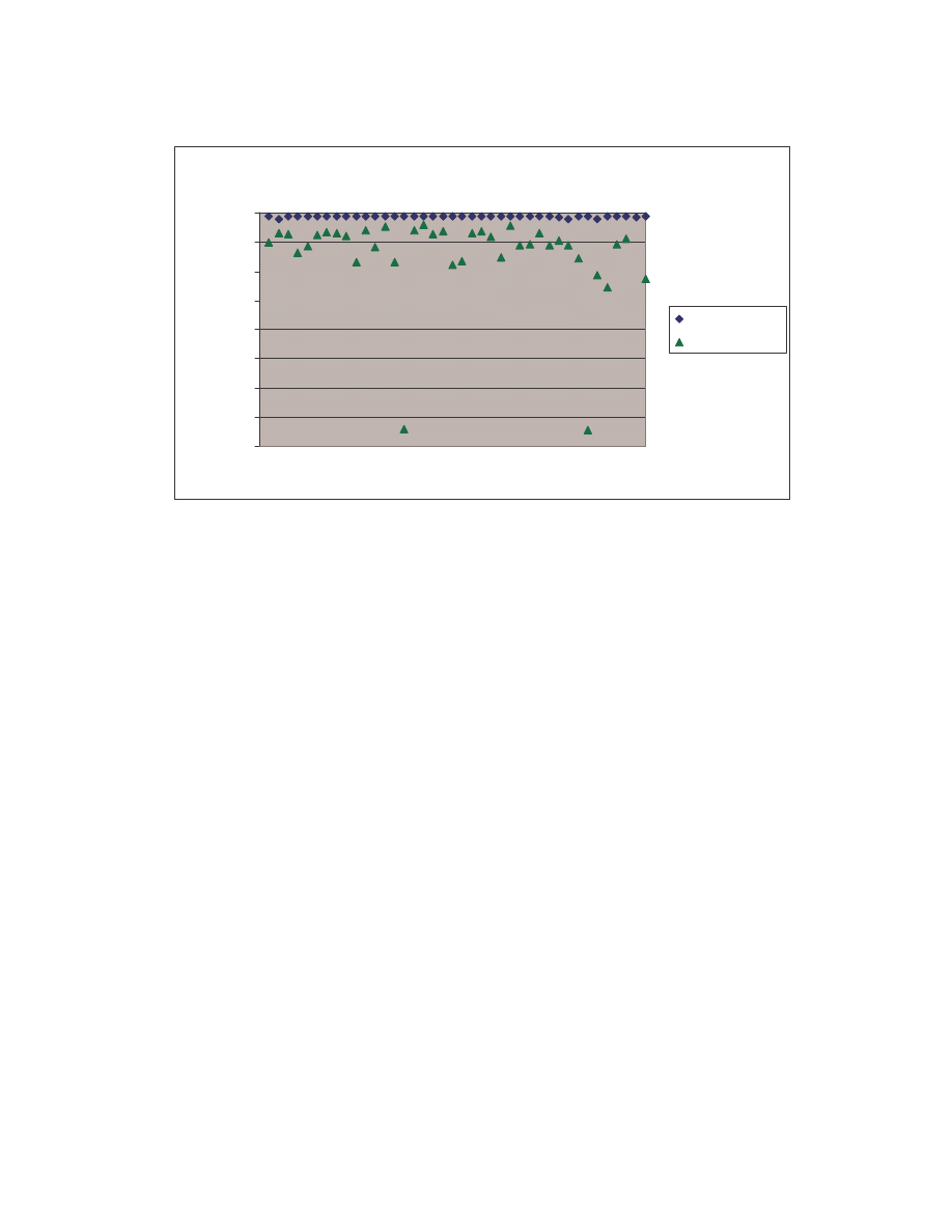
50
Test set 0, N = 2
-160
-140
-120
-100
-80
-60
-40
-20
0
0
10
20
30
40
File number
S
co
re
(
LL
P
O
)
family viruses
normal files
Figure 12 Difference in scores between family viruses and normal files.
The kind of clear separation that we saw in the previous model was typical for most
models. This is illustrated in Table 8 where for each model we compare the minimum
score of the family viruses to the maximum score of the normal files. The minimum is
higher than the maximum in most cases. Two exceptions occurred with test set 1, where
one family virus (IDA_N51) had a score that fell within the score range of the random
files, for the two models with N = 2 and 3. Other than these two cases, the models made a
clear distinction of scores between family viruses and normal programs. We can easily
distinguish a virus from a normal program by their scores in the HMMs.

51
min score of family viruses max score of normal files
N = 2
-4.4349
-8.0663
N = 3
-5.8575
-8.9071
N = 4
-4.2053
-7.9974
N = 5
-4.1830
-8.0300
N = 6
-4.0856
-8.0337
N = 2
-7.5872
-7.3842
N = 3
-9.0385
-8.0840
N = 4
-7.4071
-9.5793
N = 5
-7.3438
-7.9866
N = 6
-8.8787
-11.9263
N = 2
-4.6882
-7.9172
N = 3
-4.6185
-8.8983
N = 4
-4.4834
-11.2414
N = 5
-4.4185
-8.1327
N = 6
-4.3807
-8.5476
N = 2
-4.4981
-8.5878
N = 3
-4.3908
-8.8650
N = 4
-4.3082
-11.8215
N = 5
-4.2480
-8.6818
N = 6
-4.2215
-9.1706
N = 2
-4.3924
-7.4781
N = 3
-4.2564
-7.4590
N = 4
-4.2496
-9.5862
N = 5
-4.2261
-8.5506
N = 6
-4.1822
-7.4662
Test set 3
Test set 4
Test set 0
Test set 1
Test set 2
Table 8 Minimum score of the 40 family viruses and maximum score of the 40 normal programs
assigned by each model.
Next, we examined how the HMMs perform when we included the non-family viruses in
the comparison set. Seven of the models made a complete separation of scores between
viruses in the test set and files in the comparison set. That is, the LLPO of the family
viruses were all higher than those of the normal files as well as the non-family viruses.
For the other models, we find some overlapping of scores where some non-family viruses
have scores higher than some of the family viruses.
Figure 13 shows the result of the model with three states (i.e., N = 3) using test set 0. For
this case, the score distinction between family viruses and non-family viruses is not as
clear. Some non-family viruses in the comparison set have scores very close to or higher
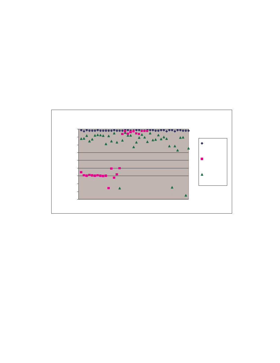
52
than the family viruses. In fact, these non-family viruses are the VCL32 viruses which we
showed in Section 3 that they possess some similarities to NGVCK viruses. Our HMMs
separated these viruses, which have some similarities to the viruses the HMMs represent,
from the other non-family viruses, which have zero similarity to the NGVCK viruses. As
is shown in Figure 13, the scores for the VCL32 viruses are much higher than the scores
for the other non-family viruses.
Test set 0, N = 3
-180
-160
-140
-120
-100
-80
-60
-40
-20
0
0
10
20
30
40
File number
S
co
re
(
LL
P
O
)
family
viruses
non-family
viruses
normal
files
Figure 13 Log likelihood per opcode (LLPO) of family viruses, non-family viruses and normal files.
The result illustrated in Figure 13 is common to most models. In fact, if we look at the
graph for each of the test sets for each N, the score distribution is very similar. If a file
has a low score in one model, it always has a low score in all other models, although the
scores are not always identical. We have included more of these graphs in Appendix B.
Table B-1 shows the models trained with N = 3 states and Table B-2 shows the models
with N = 5 states. The shapes of the curves are very similar in every graph. The raw
scores of all the test runs are listed in Table B-3 in Appendix B. Our HMMs showed
consistent performance over the test data, regardless of the number of hidden states: all

53
normal benign programs were distinguishable by their scores; non-family viruses
showing no similarity to the viruses represented by the HMMs had very low scores; and
non-family viruses having some similarities to the family viruses had scores closer to the
family viruses.
4.5.2 Threshold and False Predictions
Next we counted the number of false positives and false negatives associated with each
model. A false positive occurs when a program not belonging to the virus family
represented by an HMM is classified by the HMM as being a member virus. A false
negative occurs when a member virus is misclassified as being a non-member.
Analogously, true positives are family viruses correctly classified as members; while true
negatives are programs not belonging to the virus family correctly classified as non-
members.
Recall that a trained HMM classifies a program by comparing its log likelihood per
opcode (LLPO) to the threshold LLPO. The choice of threshold value therefore affects
the classification and thus the amount of false positives and false negatives a model
produces. If we choose a higher threshold, fewer programs would score higher than the
threshold and there would be fewer false positives. This, however, is usually
accompanied by more false negatives as more member viruses may have scores lower
than the threshold. Depending on the desired tradeoff, we could select the threshold
accordingly.
Note that the HMMs made a separation of scores between family viruses and normal
programs (except for the one virus IDA_N51). If we reasonably choose a threshold that is
lower than all family virus scores and higher than all normal file scores, no normal files
will become false positives and no family viruses will become false negatives. (And for
the two models where IDA_N51 had a score lower than some normal file, there will be
one false positive out of the 40 family viruses.) The issue of false positives, false
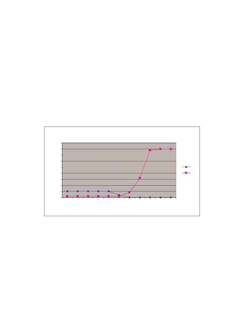
54
negatives and their tradeoff arises only when we take into account the non-family viruses,
because their score range interleaves with the family virus score range. In other words,
false positives would mainly come from the non-family viruses, particularly the VCL32
viruses as they are the only viruses that scored close to the family viruses. False negatives
occur when we adjust the threshold to reduce the number of misclassified VCL32 viruses.
We determined the amount of false positives and false negatives that came with different
threshold values. Figure 14 illustrates the tradeoff between the two when the threshold
changes from -3.5 to -2.5, for the model with N = 2 hidden states using test set 4. The
actual counts are shown in Table 9.
Test set 4, N = 2
0
5
10
15
20
25
30
35
40
45
-3.5 -3.4 -3.3 -3.2 -3.1 -3.0 -2.9 -2.8 -2.7 -2.6 -2.5
Possible threshold values
Fa
ls
e
cl
as
si
fic
at
io
ns
FP
FN
Figure 14 Tradeoff between false positives (FP) and false negatives (FN) with changing threshold
values.
55
Threshold -3.5
-3.4
-3.3
-3.2
-3.1
-3.0
-2.9
-2.8
-2.7
-2.6
-2.5
FP
5
5
5
5
5
2
0
0
0
0
0
FN
1
1
1
1
1
1
4
16
39
40
40
Table 9 False positive (FP) and false negative (FN) counts for threshold ranging from -3.5 to -2.5.
This model used test set 4 and N = 2.
4.5.3 Detection Rate, False Positive Rate, and Overall Accuracy
Besides the raw false positive and false negative counts, we calculated three other
performance measures based on these counts: detection rate, false positive rate, and
overall accuracy. The detection rate tells us the sensitivity of the model and is defined as
the number of member viruses that are caught by an HMM divided by the total number of
member viruses in the test set (40 in our experiments). The false positive rate is related to
the specificity of the model and is defined as the number of false positives divided by the
total number of non-member programs in the comparison set (65 in our test runs). Overall
accuracy is defined as the number of true predictions (positives and negatives) divided by
the total number of member and non-member programs (105 in our tests). The three
measures are related to true positives (TP), true negatives (TN), false positives (FP), and
false negatives (FN) as follows:
Detection rate =
FN
TP
TP
+
, as TP + FN equals total number of member viruses
tested;
False positive rate =
TN
FP
FP
+
, as FP + TN equals total number of non-member
programs tested;
Overall accuracy =
FN
FP
TN
TP
TN
TP
+
+
+
+
.
The detection rate, false positive rate, and overall accuracy of the test run above are
shown in Figure 15. We plotted the rates from threshold -4.5 to -2.5. The three rates are
again functions of the threshold. At a threshold value of -3.0, the detection rate and
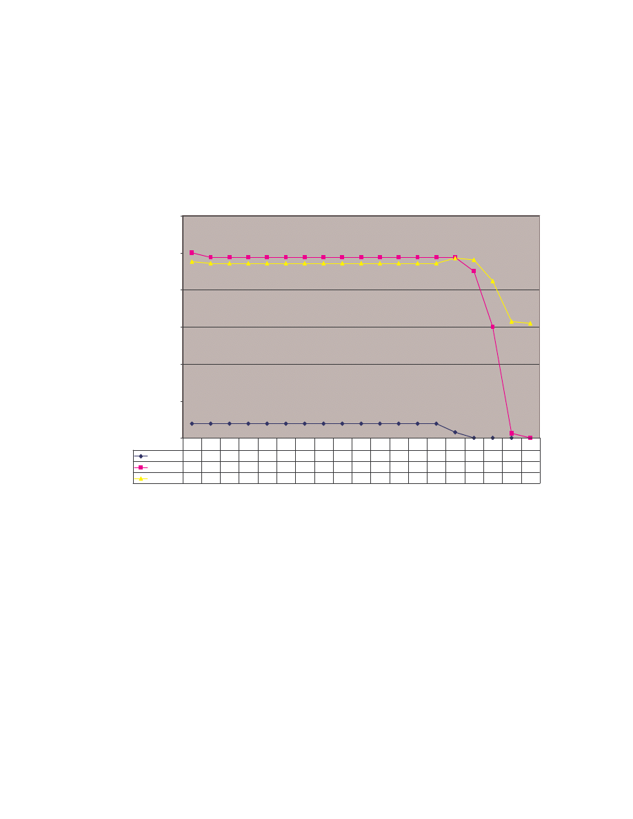
56
overall accuracy are 97.5% and 97.1% respectively while the false positive rate is 3.1%.
If we increase the threshold to -2.9, the false positive rate would be 0% but both detection
rate and accuracy would drop to 90% and 96.2%, respectively.
Test set 4, N = 2
0.0
0.2
0.4
0.6
0.8
1.0
1.2
Possible threshold values
Fa
ls
e
cl
as
si
fic
at
io
ns
FP rate
0.077 0.077 0.077 0.077 0.077 0.077 0.077 0.077 0.077 0.077 0.077 0.077 0.077 0.077 0.031 0.000 0.000 0.000 0.000
detect rate 1.000 0.975 0.975 0.975 0.975 0.975 0.975 0.975 0.975 0.975 0.975 0.975 0.975 0.975 0.975 0.900 0.600 0.025 0.000
accuracy
0.952 0.943 0.943 0.943 0.943 0.943 0.943 0.943 0.943 0.943 0.943 0.943 0.943 0.943 0.971 0.962 0.848 0.629 0.619
-4.4 -4.3 -4.2 -4.1 -4.0 -3.9 -3.8 -3.7 -3.6 -3.5 -3.4 -3.3 -3.2 -3.1 -3.0 -2.9 -2.8 -2.7 -2.6
Figure 15 Comparison of false positive rate, detection rate and overall accuracy.
Suppose we want to limit the false negative rate to 10%. In other words, we want to have
a detection rate of 90% or more. The threshold values that would produce the desired
detection performance are listed in Table 10. The value for each model is the largest
threshold LLPO that can still maintain a false negative rate of 10%. If we choose a
threshold lower than the listed value, it is possible to achieve a higher detection rate,
although it is likely that the false positive rate will also increase. The false positive rates
for all the models, at the respective threshold values, fall within 0% to 7.7%. Even the

57
detection rate and overall accuracy of all models are quite similar, the models with three
states (i.e., N = 3) produced 0% false positives with all the five test sets. In this sense,
models with three states have slightly better performance than the other models.
threshold
FP
FN
detect rate FP rate
accuracy
test set 0
-3.0
2
3
0.925
0.031
0.952
test set 1
-2.9
2
4
0.900
0.031
0.943
test set 2
-2.9
1
3
0.925
0.015
0.962
test set 3
-4.4
5
2
0.950
0.077
0.933
test set 4
-2.9
0
4
0.900
0.000
0.962
test set 0
-4.5
0
4
0.900
0.000
0.962
test set 1
-4.4
0
3
0.925
0.000
0.971
test set 2
-2.8
0
4
0.900
0.000
0.962
test set 3
-4.3
0
4
0.900
0.000
0.962
test set 4
-2.8
0
4
0.900
0.000
0.962
test set 0
-2.8
0
3
0.925
0.000
0.971
test set 1
-2.7
0
4
0.900
0.000
0.962
test set 2
-2.7
2
4
0.900
0.031
0.943
test set 3
-4.2
3
4
0.900
0.046
0.933
test set 4
-2.7
0
4
0.900
0.000
0.962
test set 0
-2.7
0
4
0.900
0.000
0.962
test set 1
-2.7
3
4
0.900
0.046
0.933
test set 2
-2.7
0
4
0.900
0.000
0.962
test set 3
-4.2
5
3
0.925
0.077
0.924
test set 4
-2.7
0
3
0.925
0.000
0.971
test set 0
-2.7
0
4
0.900
0.000
0.962
test set 1
-4.2
0
3
0.925
0.000
0.971
test set 2
-4.1
5
4
0.900
0.077
0.914
test set 3
-4.2
3
1
0.975
0.046
0.962
test set 4
-2.6
0
4
0.900
0.000
0.962
N = 4
N = 5
Detection rate >= 90%
N = 6
N = 2
N = 3
Table 10 Threshold LLPO with detection rate of 90% or more for each model.
Finally, we pick the value -4.5, which is the lowest threshold in the analysis above, and
see how the performance measures would change with this lower threshold value. Table
11 shows the false positive count, false negative count, detection rate, false positive rate
and overall accuracy when we set the cutpoint at -4.5 for all the models. Compared to the
previous table, the detection rates as well as the false positive rates indeed have increased
for most models. We see that 17 of the models have detection rate reaching 100% and 10

58
models have 0% false positive rate. Although the performance of all the models is quite
similar, models with two states (N = 2) do have slightly higher false positive rates and
lower accuracy. All models with three states (N = 3) maintain their false positive rates at
0% but their detection rates are lower than the other models. We conclude there is not a
significant difference in performance between models with three or more states.
FP
FN
detect rate
FP rate
accuracy
test set 0
5
0
1.000
0.077
0.952
test set 1
5
2
0.950
0.077
0.933
test set 2
5
2
0.950
0.077
0.933
test set 3
5
0
1.000
0.077
0.952
test set 4
5
0
1.000
0.077
0.952
test set 0
0
4
0.900
0.000
0.962
test set 1
0
2
0.950
0.000
0.981
test set 2
0
1
0.975
0.000
0.990
test set 3
0
0
1.000
0.000
1.000
test set 4
0
0
1.000
0.000
1.000
test set 0
0
0
1.000
0.000
1.000
test set 1
3
2
0.950
0.046
0.952
test set 2
5
0
1.000
0.077
0.952
test set 3
3
0
1.000
0.046
0.971
test set 4
3
0
1.000
0.046
0.971
test set 0
0
0
1.000
0.000
1.000
test set 1
5
2
0.950
0.077
0.933
test set 2
5
0
1.000
0.077
0.952
test set 3
5
0
1.000
0.077
0.952
test set 4
0
0
1.000
0.000
1.000
test set 0
0
0
1.000
0.000
1.000
test set 1
0
3
0.925
0.000
0.971
test set 2
5
0
1.000
0.077
0.952
test set 3
3
0
1.000
0.046
0.971
test set 4
5
0
1.000
0.077
0.952
N = 5
N = 6
Threshold = -4.5
N = 2
N = 3
N = 4
Table 11 False positive count, false negative count, detection rate, false positive rate and overall
accuracy when threshold is set at -4.5 for all models.
4.5.4 Run Time of the Training and Classifying Process
Training an HMM is an iterative process. As discussed in Section 4.1.2 where the HMM
algorithms were presented, each iteration consists of an -pass, a -pass, the computation
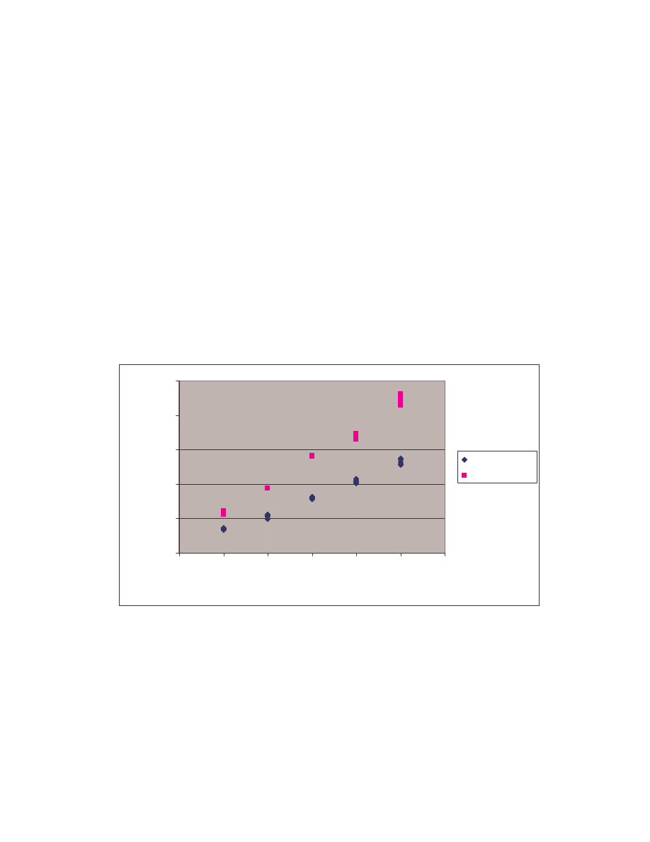
59
of the values, the re-estimation of the model parameters, and the calculation of the log
likelihood of the training sequence [18]. Each of these steps, except the calculation of log
likelihood, requires computations in the order of N
2
T, where N is the number of states in
the model and T is the length of the training sequence. Thus each iteration requires
O(N
2
T) time and the total run time is also proportional to the number of iterations taken.
We recorded the training time of the models and the result is shown in Figure 16. We
timed the trainings twice setting the maximum number of iterations to 500 and 800
respectively. T was around 66,500 for all models. With 500 iterations, training time
ranged from 5 minutes to 23 minutes. With 800 iterations, training time ranged from 9
minutes to 38 minutes depending on the number of states N.
0
500
1000
1500
2000
2500
1
2
3
4
5
6
7
Number of states N
Tr
ai
ni
ng
t
im
e
(s
ec
on
ds
)
500 iterations
800 iterations
Figure 16 Training time of the 25 models using 500 iterations and 800 iterations respectively.
Classifying a program requires the computation of its log likelihood per opcode (LLPO)
in a model. We compute this score by running the -pass, which is an O(N
2
T) inductive
process. Since the score is found in only one -pass, the scoring of a program in a HMM
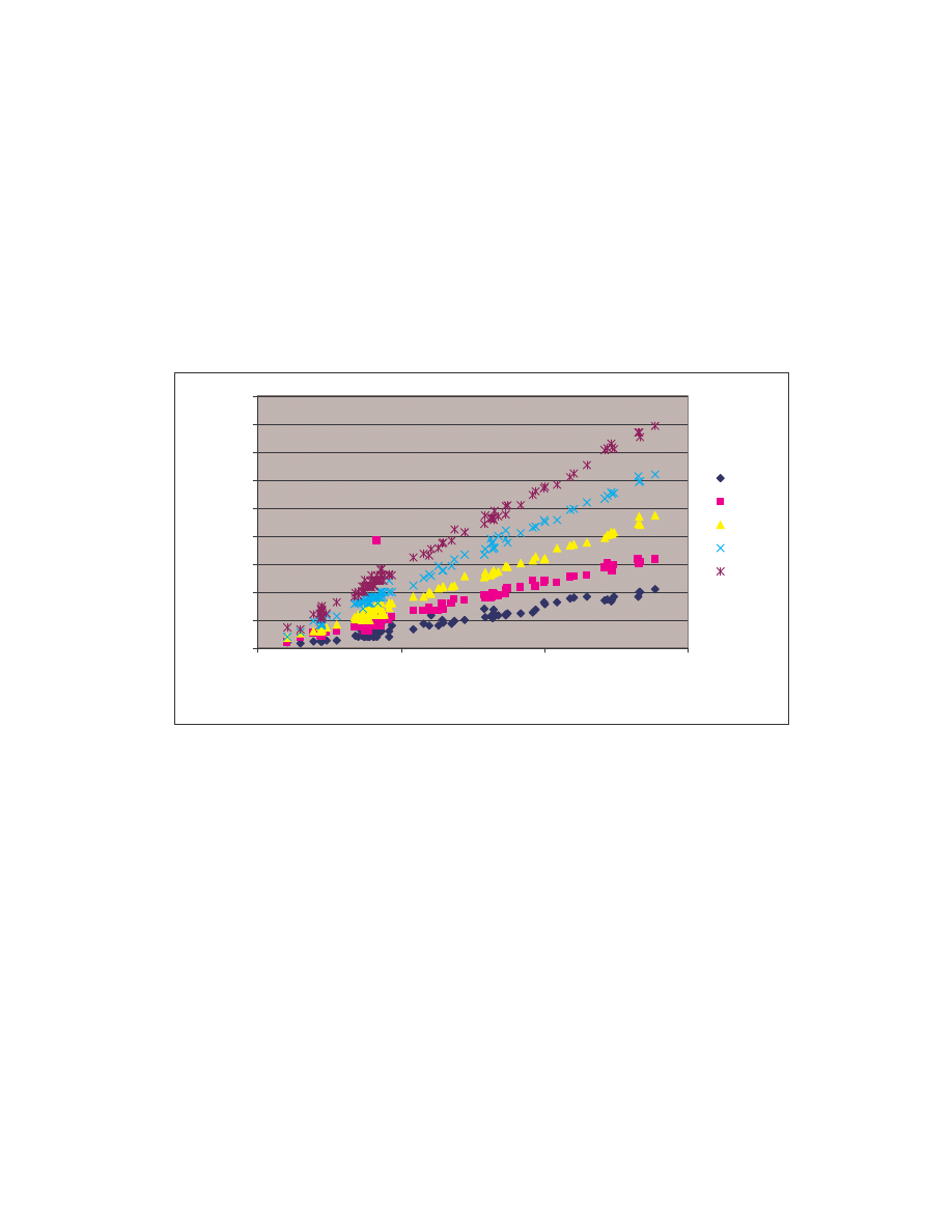
60
is relative fast, compared to the training of a model. We recorded the time it took our
models to score each of the virus files and the normal programs and plotted the result in
Figure 17. Our models can score files of any length and the length T (in number of
opcodes) of our data ranged from 100 to 1400. The time to score a program range from
0.008 milliseconds to 0.4 milliseconds, depending on the number of states N of the model
and the number of opcodes T in the program.
0
0.05
0.1
0.15
0.2
0.25
0.3
0.35
0.4
0.45
0
500
1000
1500
Length of observation sequence T
S
co
rin
g
tim
e
(m
ill
is
ec
on
ds
)
N = 2
N = 3
N = 4
N = 5
N = 6
Figure 17 Scoring time as a function of observation sequence length T and number of states N.
The algorithms for training were implemented in C and the scoring routine was written in
Ruby [16]. Each training and each scoring was let to run by itself on a Pentium M 1.4
GHz machine running Windows XP Home Edition with 768 MB of RAM.
4.6 The Trained Models
We trained the hidden Markov models (HMMs) using different number of states without
knowing how to interpret the observations and what features the viruses contain.
Theoretically, the final converged probabilities in the HMM matrices (i.e., A, B, and
π
),

61
particularly the B matrix which contains the observation probabilities of the observable
symbols (i.e., opcodes) at each state, should help us reveal the significant features of the
viruses on which the HMMs are trained. We examined the final parameters of our HMMs
to infer what the features might be. We found that the opcodes can readily be grouped
under the states. More than half of the opcodes are seen in one state only, meaning that
each of these opcodes has an observation probability of zero in all but one state. For each
of the other opcodes which has non-zero observation probabilities in more than one state,
we can still easily find the state that it belongs because one of the observation
probabilities usually stands out. In other words, the opcodes form a partition into states.
By examining the grouping of opcodes, it is possible to discover what each state
represents. Table 12 is the transpose of the converged B matrix for the model with N = 3
states using test set 0 (i.e., trained on test set 1 to 4). We sorted the opcodes by their
probabilities in state 0.

62
B:
state 0
state 1
state 2
state 0
state 1
state 2
pop
0.18166
0.00000
0.03246 dec
0.00000
0.04817
0.01547
jz
0.18012
0.00000
0.00000 movzx
0.00000
0.00000
0.01002
retn
0.15195
0.00000
0.00489 not
0.00000
0.00000
0.00621
jnz
0.12674
0.00000
0.00000 neg
0.00000
0.00000
0.00477
push
0.12364
0.38830
0.03404 imul
0.00000
0.00000
0.00385
call
0.10758
0.08648
0.04103 xchg
0.00000
0.00000
0.00279
jb
0.03760
0.00000
0.00000 movsb
0.00000
0.00000
0.00258
jmp
0.01850
0.00227
0.02770 start
0.00000
0.00349
0.00218
rcl
0.01434
0.00017
0.00122 stosd
0.00000
0.00000
0.00164
jbe
0.01141
0.00000
0.00000 rep
0.00000
0.00000
0.00144
jnb
0.01011
0.00000
0.00000 lodsw
0.00000
0.00000
0.00123
popa
0.00995
0.06472
0.00025 stosw
0.00000
0.00000
0.00116
ja
0.00597
0.00000
0.00000 lodsd
0.00000
0.00000
0.00101
lea
0.00587
0.00000
0.02525 stosb
0.00000
0.00000
0.00089
div
0.00558
0.00000
0.00207 lodsb
0.00000
0.00000
0.00087
cld
0.00307
0.00000
0.00433 loop
0.00000
0.00000
0.00046
adc
0.00219
0.00181
0.00476 in
0.00000
0.00000
0.00007
shl
0.00082
0.00000
0.01241 ins
0.00000
0.00000
0.00007
ror
0.00063
0.00000
0.00481 repe
0.00000
0.00000
0.00007
sbb
0.00058
0.00000
0.00160 std
0.00000
0.00000
0.00005
shr
0.00035
0.00010
0.00451 movsd
0.00000
0.00007
0.00003
inc
0.00017
0.01408
0.02316 popf
0.00000
0.00000
0.00002
rol
0.00016
0.00000
0.00457 fnstenv
0.00000
0.00000
0.00002
jnp
0.00015
0.00000
0.00000 scasb
0.00000
0.00000
0.00002
add
0.00013
0.01315
0.22386 cmc
0.00000
0.00000
0.00002
or
0.00013
0.02146
0.00670 enter
0.00000
0.00000
0.00002
sar
0.00013
0.00056
0.00155 jns
0.00000
0.00000
0.00002
test
0.00009
0.03124
0.00000 icebp
0.00000
0.00000
0.00002
bound
0.00008
0.00000
0.00000 jle
0.00000
0.00000
0.00002
jp
0.00008
0.00000
0.00000 cmp
0.00000
0.20651
0.00000
cmpsb
0.00008
0.00000
0.00000 clc
0.00000
0.03823
0.00000
fidiv
0.00008
0.00000
0.00000 stc
0.00000
0.02578
0.00000
retf
0.00007
0.00006
0.00003 rcr
0.00000
0.00482
0.00000
and
0.00000
0.00258
0.02054 aad
0.00000
0.00008
0.00000
mov
0.00000
0.00214
0.35145 fild
0.00000
0.00008
0.00000
sub
0.00000
0.03582
0.06531 jecxz
0.00000
0.00008
0.00000
xor
0.00000
0.00759
0.02583 out
0.00000
0.00008
0.00000
pusha
0.00000
0.00000
0.01862 hlt
0.00000
0.00008
0.00000
Table 12 The final B matrix transpose for model with N = 3 using test set 0.
In Figure 18, we graphed the probability distributions of the opcodes in Table 12. Here
we can easily see that the peaks for each state appear at different locations. Certain
opcodes are predominately seen in a particular state only. Opcodes that are mostly seen
only in state 0 include
pop, jz, retn, jnz, and call. Those that are mostly seen in state 1
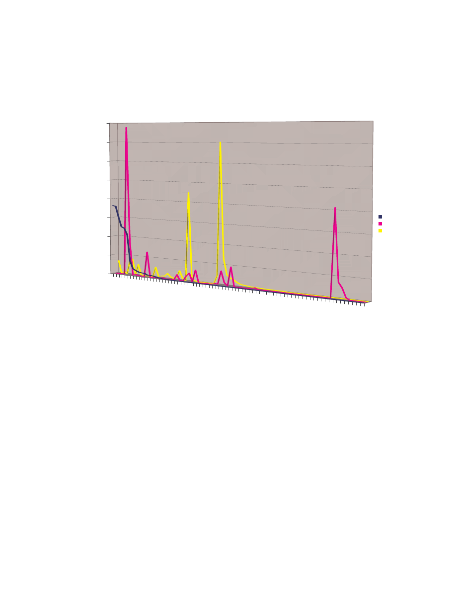
63
include
push, popa, and cmp. Opcodes that have high probabilities only in state 2 include
add and move.
po
p
re
tn
pu
sh jb rc
l
jn
b ja
di
v
ad
c
ro
r
sh
r
ro
l
ad
d
sa
r
bo
un
d
cm
ps
b
re
tf
m
ov xo
r
de
c
no
t
im
ul
m
ov
sb
st
os
d
lo
ds
w
lo
ds
d
lo
ds
b in
re
pe
m
ov
sd
fn
st
en
v
cm
c
jn
s
jle clc rcr fild
ou
t
0.00
0.05
0.10
0.15
0.20
0.25
0.30
0.35
0.40
ob
se
rv
at
io
n
pr
ob
ab
ili
ty
opcode
state 0
state 1
state 2
Figure 18 Probability distributions of observation symbols for each state in the model with N = 3
using test set 0.
To show the relative probabilities of each opcode being seen in each of the three states,
we normalize, for each opcode, its probabilities in state 0, state 1, and state 2 so that the
three observation probabilities sum to 1. The relative probabilities tell us in which state
each opcode appear mostly. Again as we can see in Figure 19, most opcodes appear in
one state only.
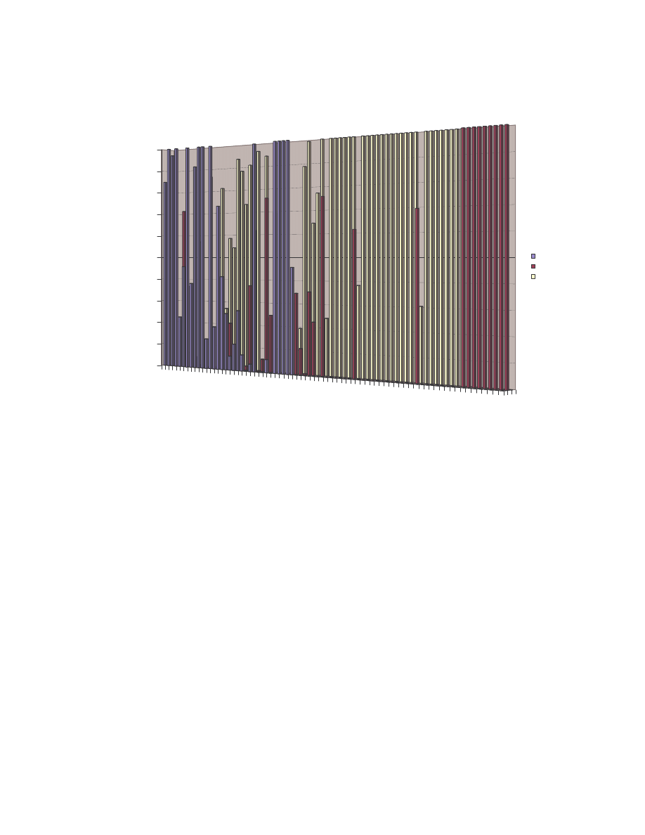
64
po
p
re
tn
pu
sh jb rcljnb jadivadc rorshr rol
ad
d
sa
r
bo
un
d
cm
ps
b
re
tf
mo
v
xo
r
de
c
no
t
im
ul
mo
vs
b
sto
sd
lod
sw
lod
sd
lod
sb in
re
pe
mo
vs
d
fns
ten
v
cm
c
jns jle clc rcr fild out
0
0.1
0.2
0.3
0.4
0.5
0.6
0.7
0.8
0.9
1
no
rm
al
iz
ed
o
bs
er
va
tio
n
pr
ob
ab
ili
tiy
opcode
state 0
state 1
state 2
Figure 19 Probabilities of each opcode in state 0, state 1, and state 2 normalized to show the
composition of states for each opcode.
The groupings of opcodes are not always the same in all our models. But that the opcodes
always form a partition remain the same for all models. We included some more
converged matrices A, B, and
π
in Appendix C.
5. DETECTION WITH SIMILARITY INDEX AND COMMERCIAL SCANNERS
5.1 Classifying by Similarity Index
In the similarity tests described in Section 3, we found that viruses generated by the Next
Generation Virus Creation Kit (NGVCK) are only about 10% similar among themselves,
on average. They share even lower similarities when compared to normal programs (0 to
1.1%), and when compared to other viruses not in the same family (0 to 5.5%). Since

65
these NGVCK-viruses are so different from other programs, benign or viral, it is possible
to distinguish them by using similarity index alone.
This straight-forward approach would work as follows. To classify whether a program
belongs to the NGVCK virus family, compare the program to any randomly chosen
NGVCK virus. If it has no similarity to the NGVCK virus, it is classified as non-family
(i.e. not belonging to the NGVCK family). Otherwise, we compare some more NGVCK
viruses to the chosen NGVCK virus to determine a threshold. If the similarity score of the
program with the original chosen NGVCK virus is higher than the threshold value, it is
classified as a family virus.
We used this approach to classify the 40 family viruses IDA_N0 to IDA_N39, the 40
normal files, and the 25 non-family viruses generated for the tests in Section 4. We ran
two tests where we compared the 105 files to IDA_N146 and IDA_N101 respectively.
The similarity scores for the test using IDA_N146 for comparison are shown in Table 13.
66
Comparing IDA_N146 to:
Threshold determination:
family
scores normal
scores non-family scores
Comparing IDA_N146 to
viruses
files
viruses
40 NGVCK viruses
IDA_N0
0.0728 IDA_R0
0
IDA_V0
0
min score
0.0349
IDA_N1
0.1133 IDA_R1
0
IDA_V1
0
max score
0.1894
IDA_N2
0.0925 IDA_R2
0
IDA_V2
0
IDA_N3
0.0684 IDA_R3
0
IDA_V3
0
IDA_N4
0.0791 IDA_R4
0
IDA_V4
0
IDA_N5
0.1162 IDA_R5
0
IDA_V5
0
IDA_N6
0.0970 IDA_R6
0
IDA_V6
0
IDA_N7
0.1376 IDA_R7
0
IDA_V7
0
IDA_N8
0.0403 IDA_R8
0
IDA_V8
0
IDA_N9
0.1764 IDA_R9
0
IDA_V9
0
IDA_N10
0.1886 IDA_R10
0
IDA_V10
0
IDA_N11
0.1390 IDA_R11
0
IDA_V11
0
IDA_N12
0.1364 IDA_R12
0
IDA_V12
0
IDA_N13
0.1462 IDA_R13
0
IDA_V13
0
IDA_N14
0.1257 IDA_R14
0
IDA_V14
0
IDA_N15
0.1066 IDA_R15
0
IDA_V15
0.0188
IDA_N16
0.1238 IDA_R16
0
IDA_V16
0.0215
IDA_N17
0.1044 IDA_R17
0
IDA_V17
0.0153
IDA_N18
0.0781 IDA_R18
0
IDA_V18
0.0163
IDA_N19
0.1172 IDA_R19
0
IDA_V19
0.0235
IDA_N20
0.1052 IDA_R20
0
IDA_V20
0.0146
IDA_N21
0.1456 IDA_R21
0
IDA_V21
0.0184
IDA_N22
0.1379 IDA_R22
0
IDA_V22
0.0188
IDA_N23
0.0967 IDA_R23
0
IDA_V23
0.0192
IDA_N24
0.0871 IDA_R24
0
IDA_V24
0.0190
IDA_N25
0.1041 IDA_R25
0
IDA_N26
0.1327 IDA_R26
0
IDA_N27
0.0597 IDA_R27
0
IDA_N28
0.1667 IDA_R28
0
IDA_N29
0.0813 IDA_R29
0
IDA_N30
0.0383 IDA_R30
0
IDA_N31
0.1386 IDA_R31
0
IDA_N32
0.0999 IDA_R32
0
IDA_N33
0.0661 IDA_R33
0
IDA_N34
0.1243 IDA_R34
0.0175
IDA_N35
0.1021 IDA_R35
0
IDA_N36
0.1010 IDA_R36
0
IDA_N37
0.0845 IDA_R37
0
IDA_N38
0.0549 IDA_R38
0
IDA_N39
0.1292 IDA_R39
0
Table 13 Similarity scores between IDA_N146 and other programs including NGVCK viruses, non-
NGVCK viruses, and normal programs.
The column on the right in Table 13 shows the minimum score and the maximum score
when IDA_N146 was compared to some other NGVCK viruses. Suppose we simply used
the minimum score of 0.0349 as the threshold, we were able to correctly classify all the

67
105 files. All family viruses had scores greater than 0.0349 while all other programs
scored lower than the threshold value. In other words, the detection rate was 100% and
false positive rate was 0% in this test.
The test using IDA_N101 for comparison also achieved a 100% detection rate and a 0%
false positive rate when we used the same criteria to set the threshold. The scores for this
test are shown in Table D-1 in Appendix D. This straight-forward approach, which uses
similarity index for classification, worked remarkably well in our two tests. Accuracy
was 100% and there were no false positives or false negatives in either case.
5.2 Detection by Virus Scanners
Finally, we tested whether the NGVCK viruses can be detected by commercial virus
scanners. We stored 37 virus executables in a disk folder and scanned the folder using
three different scanners:
eTrust version 7.0.405 [5],
avast antivirus version 4.7 [2], and
AVG Anti-Virus version 7.1 [3].
The 37 viruses were all used in our HMM tests in Section 4. The executables included:
10 EXE files from the NGVCK (Next Generation Virus Creation Kit) viruses;
10 COM files from the G2 (Second Generation virus generator) viruses;
10 EXE files from the VCL32 (Virus Creation Lab for Win32) viruses; and
7 COM files from the MPCGEN (Mass Code Generator) viruses, which were in
fact PS-MPC (Phalcom/Skism Mass-Produced Code Generator) viruses as
MPCGEN runs PS-MPC within its code after it generates some random
configuration files (cfg files).
eTrust and avast detected 17 viruses, which are the G2 viruses and the MPCGEN viruses,
but not the ones generated by VCL32 and NGVCK. AVG Anti-Virus detected 27 viruses,
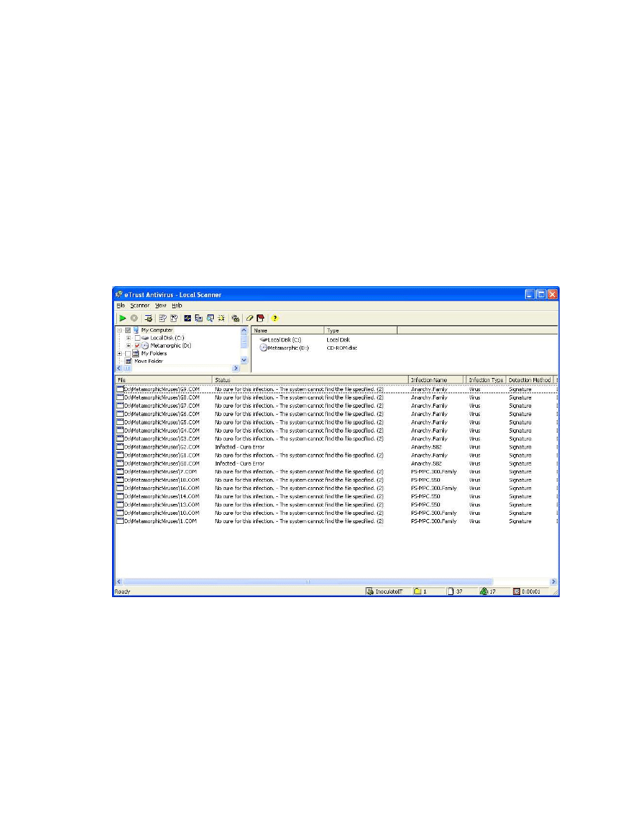
68
which are the G2, MPCGEN, and VCL32 viruses. The 10 NGVCK viruses were not
detected by either scanner.
Figure 20 is a screen capture of the eTrust test result. As shown in the figure, the
detection method used was signature. The G2 viruses were identified as the “Anarchy
Family” while the MPCGEN viruses were correctly classified as the “PS-MPC Family”.
Avast antivirus named all MPCGEN virus infections as “PS/MPC-gen” and all G2 virus
infections as “PS/G2-B”.
Figure 20 Screen capture of the eTrust scanning result on the 37 virus executables.
Figure 21 is the AVG test result. Of the seven MPCGEN viruses, three were reported as
“Could be infected PS-MPC” while the other four plus nine of the G2 viruses were
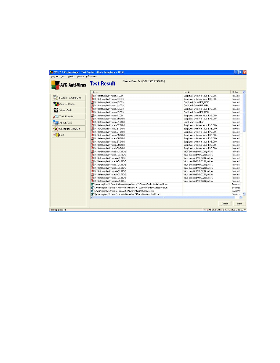
69
shown as unknown viruses. The scanner misclassified all VCL32 viruses as
“Win32/Ngvck.W” while none of the NGVCK viruses was actually detected.
Figure 21 Test result for AVG Anti-Virus on the 37 virus executables.
NGVCK viruses were able to escape detection by the scanners we tested. However, as we
have shown, both the similarity index approach and the hidden Markov model approach
were able to identify them with high accuracy. We conclude that these two methods are
very effective in dealing with NGVCK viruses.
6. CONCLUSION
Virus writers and anti-virus researchers generally agree that metamorphism is the way to
generate undetectable viruses. Several virus writers have released virus creation kits and

70
claimed that they possess the ability to automatically produce morphed virus variants that
look substantially different from one another.
To see how effective these code morphing engines are, and how much difference exists
between variants of a given virus, we measured the similarity between virus variants
generated by four virus generators downloaded from the Internet. Our results show that
the effectiveness of these generators varies widely. While the best generator, Next
Generation Virus Creation Kit (NGVCK), is able to create viruses that share only a few
percent of similarity, the other generators produce viruses that are over 60% similar, on
average. In addition, our similarity graphs show that some of these variant pairs have
long segments of identical assembly opcodes at identical positions of the virus files.
Compared to random utility files which have a similarity of about 35%, we see that some
of the virus creation kits do not effectively morph the viral code.
Not only do NGVCK viruses show low similarity among themselves, they show even
lower similarities when compared to viruses generated by other generators (from 0 to
5.5%). When compared to normal random files, the similarity scores are almost always
zero, with only a few exceptions. We conclude that NGVCK viruses have the highest
degree of metamorphism among the four virus families we tested. In addition, NGVCK
viruses are very different from normal programs and viruses in other families.
To detect metamorphic virus variants, we experimented with hidden Markov models
(HMMs) to capture the statistical properties of viruses in the same family. We generated
200 NGVCK viruses, trained 25 models and used the trained models to classify both
viruses and random non-viral programs. Of the 25 models, 23 were able to identify all the
normal programs by their scores alone. This means we can easily distinguish a NGVCK
virus from a normal program.

71
The models also distinguished between VCL32 (Virus Creation Lab for Win32) viruses
and other viruses not belonging to the NGVCK family. They assigned higher scores to
VCL32 viruses, which were the only viruses we tested that have some similarities to the
NGVCK family. Even so, seven of our models were able to perfectly distinguish the
NGVCK viruses from the VCL32 viruses by scores. The other models produced different
number of false positives and false negatives, depending on the threshold used in the
classifying process. Using -4.5 as the threshold, 17 of the models achieved a 100%
detection rate, with a false positive rate ranging from 0% to 7.7%.
If the variants of a metamorphic virus are sufficiently different that signature-based
scanning cannot detect a newly morphed variant, the HMM approach provides a feasible
solution. As with any statistical detection method, false predictions are possible. In our
tests, false positives were all due to viruses from a different family than those in the
training set, rather than normal non-viral programs. Therefore, we can view these false
positives in a positive light, since the HMM detects additional viruses which have
statistical properties similar to the viruses that the HMMs represent.
The number of states N of a model does not seem to have much impact on the
performance of the HMM. We saw only small differences in the performance measures
for models with N from 3 to 6. Since the time to train a model and the time to score a
program increases with the number of states N, we may want to use a smaller N if time is
crucial to the detection process. The trained models grouped the observed opcodes under
the hidden states according to the probabilities that they were seen. This should help us
infer features of the NGVCK viruses.
The fact that NGVCK viruses have assembly code structures that are different from
normal programs and other viruses makes them distinguishable by our straight-forward
similarity index alone. Our two tests that used similarity indices to classify 105 programs
were both 100% accurate. This result illustrates that even though the NGVCK viruses

72
show a high degree of metamorphism, it is still relatively easy to detect them since they
are “too different” from normal programs. The similarity index approach is remarkably
effective when the virus code structure is significantly different from normal non-viral
code.
We scanned the viruses from the four families with three virus scanners. Viruses in the
three families other than the NGVCK were detected by the three scanners. All NGVCK
viruses escaped detection by these signature-based scanners. While the NGVCK viruses
were not detected by the scanners we tested, we have shown that both the similarity index
approach and the HMM approach are very effective in dealing with these viruses.
For viruses to avoid detection, they not only need a high degree of metamorphism, but
also a degree of similarity to normal programs. None of the virus construction kits we
tested satisfy both of these requirements. Three of the four virus generators fall short on
metamorphism, while the one generator that is highly metamorphic lacks sufficient
similarity to non-viral code. As a result, all these viruses are relatively easy to detect. An
interesting open question is whether it is possible to satisfy both metamorphic and
similarity conditions and thereby create a truly undetectable virus.
7. FUTURE WORK
We trained our models on disassembled virus executables. The disassembling process can
take some time and the results depend on the quality of the disassembler. To speed up
virus pre-processing and to eliminate the reliance on a particular disassembler, we could
attempt to train the HMMs directly on the binary code of the viruses. Other machine
learning techniques, such as data mining or neural networks, might also work directly on
the binaries.
Training on raw executable byte sequences is more challenging as these byte sequences
are longer and contain more irrelevant parts. We can train the models using only the code

73
segments and perhaps the data segments, excluding header and other kinds of
identification information, since the behavior of a program is primarily determined by its
code segments.
To more thoroughly evaluate the performance of the HMM approach, it would be useful
to test on a larger set of virus variants and also test on different types of viruses. Ideally,
we would like to find viruses that are similar to normal programs to a degree that the
similarity index alone cannot distinguish the viruses from normal code. Only with such
data can we evaluate the effectiveness of the HMM approach to detecting metamorphic
viruses. However, it appears that no metamorphic kit available today is capable of
producing such challenging viral code.

74
Bibliography
[1]
W. Arnold, G. Tesauro, “Automatically Generated Win32 Heuristic Virus
Detection”, Proceedings of the 2000 International Virus Bulletin Conference, 2000.
[2]
avast! antivirus <http://www.avast.com/>
[3]
AVG Anti-Virus <http://www.grisoft.com/doc/1>
[4]
Cygwin <http://cygwin.com/>
[5]
eTrust by Computer Associates International, Inc.
<http://www3.ca.com/solutions/Solution.aspx?ID=271>
[6]
IDA Pro Disassembler <http://www.datarescue.com/idabase/>
[7]
R.S. Jensen, “Immune System for Virus Detection and Elimination”, master’s
thesis, Informatics and Mathematical Modelling, Technical University of Denmark,
IMM-EP-2002-55, 2002.
< www2.imm.dtu.dk/pubdb/views/edoc_download.php/959/pdf/imm959.pdf >
[8]
J. Kephart, A. William, “Automatic Extraction of Computer Virus Signatures”,
Proceedings of the 4
th
International Virus Bulletin Conference, R. Ford, ed., Virus
Bulletin Ltd., Abingdon, England, pp. 178-184, 1994.
<http://www.research.ibm.com/antivirus/SciPapers/Kephart/VB94/vb94.html>
[9]
R. Kohavi, “A study of cross-validation and bootstrap for accuracy estimation and
model selection”, Proceedings of the Fourth International Joint Conference on
Artificial Intelligence, pp. 1137-1143, 1995.
[10]
A. Krogh, “An introduction to hidden Markov models for biological sequences”,
Computational Methods in Molecular Biology, pp. 45-63, Elsevier, 1998.
[11]
A. Krogh, M. Brown, I.S. Mian, K. Sjolander, D. Haussler, “Hidden markov models
in computational biology: applications to protein modeling”, J. Mol. Biol., vol. 235,
no. 5, pp. 1501-1531, 1994.
[12]
P. Mishra, “A taxonomy of software uniqueness transformations”, master’s thesis,
San Jose State University, Dec. 2003.
<http://home.earthlink.net/~mstamp1/mss_v.html#masters>

75
[13]
M. Mohammed, “Zeroing in on metamorphic computer viruses”, master’s thesis,
University of Louisiana at Lafayette, Dec. 2003.
<http://www.cacs.louisiana.edu/~arun/papers/moin-mohammed-thesis-
dec2003.pdf>
[14]
I. Muttik, “Silicon Implants”, Virus Bulletin, pp. 8-10, May 1997.
[15]
L.R. Rabiner, “A tutorial on hidden Markov models and selected applications in
speech recognition”, Proceedings of the IEEE, vol. 77, no. 2, pp. 257-286, Feb.
1989
.
[16]
Ruby <http://www.ruby-lang.org/en/20020102.html>
[17]
M.G. Schultz, E. Eskin, E. Zadok, S.J. Stolfo, "Data Mining
Methods for Detection
of New Malicious Executables", sp, pp. 0038, IEEE Symposium on Security and
Privacy, 2001.
[18]
M. Stamp, “A Revealing Introduction to Hidden Markov Models”, January 2004.
<http://www.cs.sjsu.edu/faculty/stamp/RUA/HMM.pdf>
[19]
P. Szor, The Art of Computer Virus Research and Defense, Addison-Wesley, 2005.
[20]
P. Szor, P. Ferrie, “Hunting for Metamorphic”, Symantec Security Response.
<http://enterprisesecurity.symantec.com/PDF/metamorphic.pdf>
[21]
G. Tesauro, J.O. Kephart, G.B. Sorkin, “Neural networks for computer virus
recognition”, IEEE Expert, vol. 11, no. 4, pp. 5-6, Aug. 1996.
<http://www.research.ibm.com/antivirus/SciPapers/Tesauro/NeuralNets.html>
[22]
VX Heavens. <http://vx.netlux.org/>
[23]
washingtonpost.com Staff Writer, “A Short History of Computer Viruses and
Attacks”, Feb. 2003. <http://www.washingtonpost.com/wp-dyn/articles/A50636-
2002Jun26.html>
[24]
Zombie, “About Permutation”, documentation of RPME permutation engine.
<http://vx.netlux.org/vx.php?id=er05>
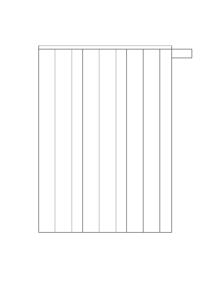
76
Appendix A: Virus similarity test results
Table A-1 Similarity scores between NGVCK virus variants.
IDA_NGVCK0 IDA_NGVCK1
0.07434 IDA_NGVCK3 IDA_NGVCK13 0.10067 IDA_NGVCK8 IDA_NGVCK11
0.07875
min
0.02934
IDA_NGVCK0 IDA_NGVCK2
0.08920 IDA_NGVCK3 IDA_NGVCK14 0.10554 IDA_NGVCK8 IDA_NGVCK12
0.03634
max
0.17176
IDA_NGVCK0 IDA_NGVCK3
0.15131 IDA_NGVCK3 IDA_NGVCK15 0.08981 IDA_NGVCK8 IDA_NGVCK13
0.03600 average 0.09600
IDA_NGVCK0 IDA_NGVCK4
0.18340 IDA_NGVCK3 IDA_NGVCK16 0.13886 IDA_NGVCK8 IDA_NGVCK14
0.02934
IDA_NGVCK0 IDA_NGVCK5
0.09070 IDA_NGVCK3 IDA_NGVCK17 0.14873 IDA_NGVCK8 IDA_NGVCK15
0.07818
IDA_NGVCK0 IDA_NGVCK6
0.05134 IDA_NGVCK3 IDA_NGVCK18 0.13848 IDA_NGVCK8 IDA_NGVCK16
0.04610
IDA_NGVCK0 IDA_NGVCK7
0.05413 IDA_NGVCK3 IDA_NGVCK19 0.12308 IDA_NGVCK8 IDA_NGVCK17
0.04854
IDA_NGVCK0 IDA_NGVCK8
0.11911 IDA_NGVCK4 IDA_NGVCK5
0.08773 IDA_NGVCK8 IDA_NGVCK18
0.06508
IDA_NGVCK0 IDA_NGVCK9
0.09770 IDA_NGVCK4 IDA_NGVCK6
0.10706 IDA_NGVCK8 IDA_NGVCK19
0.13540
IDA_NGVCK0 IDA_NGVCK10 0.12208 IDA_NGVCK4 IDA_NGVCK7
0.11275 IDA_NGVCK9 IDA_NGVCK10
0.15118
IDA_NGVCK0 IDA_NGVCK11 0.17967 IDA_NGVCK4 IDA_NGVCK8
0.07676 IDA_NGVCK9 IDA_NGVCK11
0.11877
IDA_NGVCK0 IDA_NGVCK12 0.14436 IDA_NGVCK4 IDA_NGVCK9
0.09182 IDA_NGVCK9 IDA_NGVCK12
0.09489
IDA_NGVCK0 IDA_NGVCK13 0.10156 IDA_NGVCK4 IDA_NGVCK10 0.18537 IDA_NGVCK9 IDA_NGVCK13
0.13758
IDA_NGVCK0 IDA_NGVCK14 0.12691 IDA_NGVCK4 IDA_NGVCK11 0.05152 IDA_NGVCK9 IDA_NGVCK14
0.09824
IDA_NGVCK0 IDA_NGVCK15 0.09563 IDA_NGVCK4 IDA_NGVCK12 0.10682 IDA_NGVCK9 IDA_NGVCK15
0.11261
IDA_NGVCK0 IDA_NGVCK16 0.13088 IDA_NGVCK4 IDA_NGVCK13 0.06559 IDA_NGVCK9 IDA_NGVCK16
0.16471
IDA_NGVCK0 IDA_NGVCK17 0.09841 IDA_NGVCK4 IDA_NGVCK14 0.17728 IDA_NGVCK9 IDA_NGVCK17
0.07887
IDA_NGVCK0 IDA_NGVCK18 0.12794 IDA_NGVCK4 IDA_NGVCK15 0.13155 IDA_NGVCK9 IDA_NGVCK18
0.10710
IDA_NGVCK0 IDA_NGVCK19 0.07873 IDA_NGVCK4 IDA_NGVCK16 0.10552 IDA_NGVCK9 IDA_NGVCK19
0.15248
IDA_NGVCK1 IDA_NGVCK2
0.08636 IDA_NGVCK4 IDA_NGVCK17 0.10273 IDA_NGVCK10 IDA_NGVCK11
0.10869
IDA_NGVCK1 IDA_NGVCK3
0.10922 IDA_NGVCK4 IDA_NGVCK18 0.07407 IDA_NGVCK10 IDA_NGVCK12
0.17176
IDA_NGVCK1 IDA_NGVCK4
0.16578 IDA_NGVCK4 IDA_NGVCK19 0.11025 IDA_NGVCK10 IDA_NGVCK13
0.08110
IDA_NGVCK1 IDA_NGVCK5
0.09711 IDA_NGVCK5 IDA_NGVCK6
0.05343 IDA_NGVCK10 IDA_NGVCK14
0.15890
IDA_NGVCK1 IDA_NGVCK6
0.12297 IDA_NGVCK5 IDA_NGVCK7
0.07103 IDA_NGVCK10 IDA_NGVCK15
0.16645
IDA_NGVCK1 IDA_NGVCK7
0.09787 IDA_NGVCK5 IDA_NGVCK8
0.12342 IDA_NGVCK10 IDA_NGVCK16
0.12996
IDA_NGVCK1 IDA_NGVCK8
0.07977 IDA_NGVCK5 IDA_NGVCK9
0.12222 IDA_NGVCK10 IDA_NGVCK17
0.11580
IDA_NGVCK1 IDA_NGVCK9
0.19684 IDA_NGVCK5 IDA_NGVCK10 0.07149 IDA_NGVCK10 IDA_NGVCK18
0.06672
IDA_NGVCK1 IDA_NGVCK10 0.17116 IDA_NGVCK5 IDA_NGVCK11 0.12851 IDA_NGVCK10 IDA_NGVCK19
0.04028
IDA_NGVCK1 IDA_NGVCK11 0.10572 IDA_NGVCK5 IDA_NGVCK12 0.06257 IDA_NGVCK11 IDA_NGVCK12
0.05686
IDA_NGVCK1 IDA_NGVCK12 0.11574 IDA_NGVCK5 IDA_NGVCK13 0.03453 IDA_NGVCK11 IDA_NGVCK13
0.14430
IDA_NGVCK1 IDA_NGVCK13 0.11579 IDA_NGVCK5 IDA_NGVCK14 0.05849 IDA_NGVCK11 IDA_NGVCK14
0.12858
IDA_NGVCK1 IDA_NGVCK14 0.14021 IDA_NGVCK5 IDA_NGVCK15 0.05950 IDA_NGVCK11 IDA_NGVCK15
0.14992
IDA_NGVCK1 IDA_NGVCK15 0.08796 IDA_NGVCK5 IDA_NGVCK16 0.05158 IDA_NGVCK11 IDA_NGVCK16
0.13306
IDA_NGVCK1 IDA_NGVCK16 0.07606 IDA_NGVCK5 IDA_NGVCK17 0.10532 IDA_NGVCK11 IDA_NGVCK17
0.11945
IDA_NGVCK1 IDA_NGVCK17 0.09617 IDA_NGVCK5 IDA_NGVCK18 0.06744 IDA_NGVCK11 IDA_NGVCK18
0.10001
IDA_NGVCK1 IDA_NGVCK18 0.11478 IDA_NGVCK5 IDA_NGVCK19 0.16166 IDA_NGVCK11 IDA_NGVCK19
0.11414
IDA_NGVCK1 IDA_NGVCK19 0.11744 IDA_NGVCK6 IDA_NGVCK7
0.07618 IDA_NGVCK12 IDA_NGVCK13
0.03950
IDA_NGVCK2 IDA_NGVCK3
0.11767 IDA_NGVCK6 IDA_NGVCK8
0.06070 IDA_NGVCK12 IDA_NGVCK14
0.11242
IDA_NGVCK2 IDA_NGVCK4
0.10050 IDA_NGVCK6 IDA_NGVCK9
0.10760 IDA_NGVCK12 IDA_NGVCK15
0.12866
IDA_NGVCK2 IDA_NGVCK5
0.08412 IDA_NGVCK6 IDA_NGVCK10 0.15063 IDA_NGVCK12 IDA_NGVCK16
0.03688
IDA_NGVCK2 IDA_NGVCK6
0.05393 IDA_NGVCK6 IDA_NGVCK11 0.07058 IDA_NGVCK12 IDA_NGVCK17
0.05149
IDA_NGVCK2 IDA_NGVCK7
0.12356 IDA_NGVCK6 IDA_NGVCK12 0.08605 IDA_NGVCK12 IDA_NGVCK18
0.10002
IDA_NGVCK2 IDA_NGVCK8
0.10744 IDA_NGVCK6 IDA_NGVCK13 0.06433 IDA_NGVCK12 IDA_NGVCK19
0.09563
IDA_NGVCK2 IDA_NGVCK9
0.04529 IDA_NGVCK6 IDA_NGVCK14 0.08921 IDA_NGVCK13 IDA_NGVCK14
0.09217
IDA_NGVCK2 IDA_NGVCK10 0.11901 IDA_NGVCK6 IDA_NGVCK15 0.03582 IDA_NGVCK13 IDA_NGVCK15
0.08607
IDA_NGVCK2 IDA_NGVCK11 0.04575 IDA_NGVCK6 IDA_NGVCK16 0.07146 IDA_NGVCK13 IDA_NGVCK16
0.04954
IDA_NGVCK2 IDA_NGVCK12 0.06784 IDA_NGVCK6 IDA_NGVCK17 0.15974 IDA_NGVCK13 IDA_NGVCK17
0.13265
IDA_NGVCK2 IDA_NGVCK13 0.01493 IDA_NGVCK6 IDA_NGVCK18 0.08771 IDA_NGVCK13 IDA_NGVCK18
0.05564
IDA_NGVCK2 IDA_NGVCK14 0.11570 IDA_NGVCK6 IDA_NGVCK19 0.05652 IDA_NGVCK13 IDA_NGVCK19
0.07022
IDA_NGVCK2 IDA_NGVCK15 0.09738 IDA_NGVCK7 IDA_NGVCK8
0.10729 IDA_NGVCK14 IDA_NGVCK15
0.16591
IDA_NGVCK2 IDA_NGVCK16 0.06714 IDA_NGVCK7 IDA_NGVCK9
0.09201 IDA_NGVCK14 IDA_NGVCK16
0.09793
IDA_NGVCK2 IDA_NGVCK17 0.02224 IDA_NGVCK7 IDA_NGVCK10 0.17010 IDA_NGVCK14 IDA_NGVCK17
0.09638
IDA_NGVCK2 IDA_NGVCK18 0.05040 IDA_NGVCK7 IDA_NGVCK11 0.12210 IDA_NGVCK14 IDA_NGVCK18
0.06559
IDA_NGVCK2 IDA_NGVCK19 0.08155 IDA_NGVCK7 IDA_NGVCK12 0.04414 IDA_NGVCK14 IDA_NGVCK19
0.08164
IDA_NGVCK3 IDA_NGVCK4
0.14915 IDA_NGVCK7 IDA_NGVCK13 0.08843 IDA_NGVCK15 IDA_NGVCK16
0.14119
IDA_NGVCK3 IDA_NGVCK5
0.13363 IDA_NGVCK7 IDA_NGVCK14 0.21018 IDA_NGVCK15 IDA_NGVCK17
0.03772
IDA_NGVCK3 IDA_NGVCK6
0.15358 IDA_NGVCK7 IDA_NGVCK15 0.17078 IDA_NGVCK15 IDA_NGVCK18
0.08714
IDA_NGVCK3 IDA_NGVCK7
0.14616 IDA_NGVCK7 IDA_NGVCK16 0.09845 IDA_NGVCK15 IDA_NGVCK19
0.08801
IDA_NGVCK3 IDA_NGVCK8
0.05070 IDA_NGVCK7 IDA_NGVCK17 0.11370 IDA_NGVCK16 IDA_NGVCK17
0.08680
IDA_NGVCK3 IDA_NGVCK9
0.13307 IDA_NGVCK7 IDA_NGVCK18 0.08161 IDA_NGVCK16 IDA_NGVCK18
0.03431
IDA_NGVCK3 IDA_NGVCK10 0.13738 IDA_NGVCK7 IDA_NGVCK19 0.14470 IDA_NGVCK16 IDA_NGVCK19
0.04922
IDA_NGVCK3 IDA_NGVCK11 0.13700 IDA_NGVCK8 IDA_NGVCK9
0.12738 IDA_NGVCK17 IDA_NGVCK18
0.06581
IDA_NGVCK3 IDA_NGVCK12 0.05351 IDA_NGVCK8 IDA_NGVCK10 0.10699 IDA_NGVCK17 IDA_NGVCK19
0.15762
IDA_NGVCK18 IDA_NGVCK19
0.08161
Similarity scores between files:
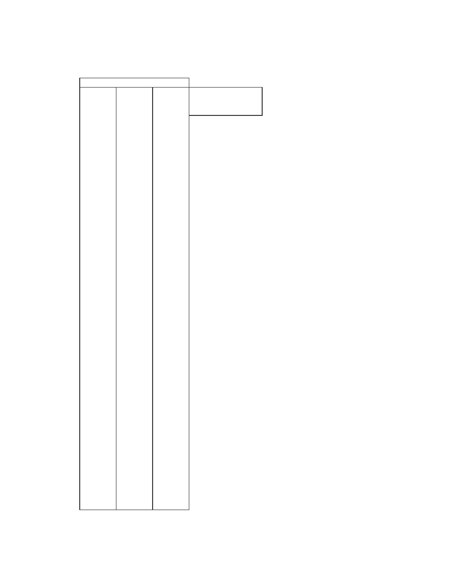
77
Table A-2 Similarity scores between G2 virus variants.
Similarity scores between files:
IDA_G0
IDA_G1
0.70808
min
0.62845
IDA_G0
IDA_G2
0.79452
max
0.84864
IDA_G0
IDA_G3
0.79818 average
0.74491
IDA_G0
IDA_G4
0.70615
IDA_G0
IDA_G5
0.73516
IDA_G0
IDA_G6
0.64831
IDA_G0
IDA_G7
0.77626
IDA_G0
IDA_G8
0.73685
IDA_G0
IDA_G9
0.68037
IDA_G1
IDA_G2
0.72647
IDA_G1
IDA_G3
0.77599
IDA_G1
IDA_G4
0.66519
IDA_G1
IDA_G5
0.80004
IDA_G1
IDA_G6
0.76389
IDA_G1
IDA_G7
0.78624
IDA_G1
IDA_G8
0.78343
IDA_G1
IDA_G9
0.72187
IDA_G2
IDA_G3
0.68350
IDA_G2
IDA_G4
0.71527
IDA_G2
IDA_G5
0.71690
IDA_G2
IDA_G6
0.67589
IDA_G2
IDA_G7
0.78995
IDA_G2
IDA_G8
0.76888
IDA_G2
IDA_G9
0.76256
IDA_G3
IDA_G4
0.71857
IDA_G3
IDA_G5
0.84864
IDA_G3
IDA_G6
0.79908
IDA_G3
IDA_G7
0.62845
IDA_G3
IDA_G8
0.78621
IDA_G3
IDA_G9
0.67891
IDA_G4
IDA_G5
0.76994
IDA_G4
IDA_G6
0.67437
IDA_G4
IDA_G7
0.75171
IDA_G4
IDA_G8
0.78997
IDA_G4
IDA_G9
0.80183
IDA_G5
IDA_G6
0.79544
IDA_G5
IDA_G7
0.71690
IDA_G5
IDA_G8
0.84669
IDA_G5
IDA_G9
0.75799
IDA_G6
IDA_G7
0.78165
IDA_G6
IDA_G8
0.76960
IDA_G6
IDA_G9
0.73567
IDA_G7
IDA_G8
0.67735
IDA_G7
IDA_G9
0.76256
IDA_G8
IDA_G9
0.70939
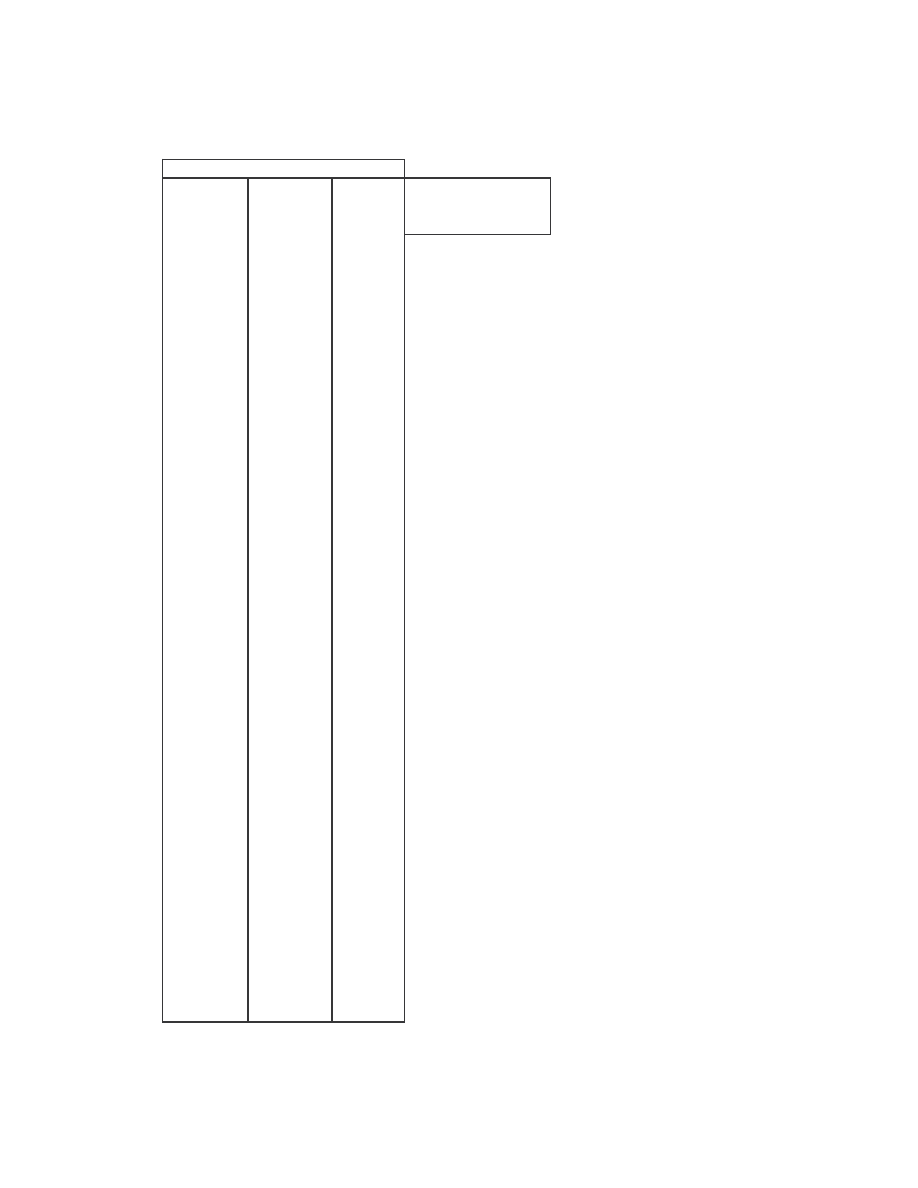
78
Table A-3 Similarity scores between VCL32 virus variants.
Similarity scores between files:
IDA_VCL0 IDA_VCL1
0.66883
min
0.34376
IDA_VCL0 IDA_VCL2
0.71341
max
0.92907
IDA_VCL0 IDA_VCL3
0.40061 average
0.60631
IDA_VCL0 IDA_VCL4
0.81177
IDA_VCL0 IDA_VCL5
0.63669
IDA_VCL0 IDA_VCL6
0.80079
IDA_VCL0 IDA_VCL7
0.41714
IDA_VCL0 IDA_VCL8
0.56377
IDA_VCL0 IDA_VCL9
0.60213
IDA_VCL1 IDA_VCL2
0.43906
IDA_VCL1 IDA_VCL3
0.65971
IDA_VCL1 IDA_VCL4
0.81516
IDA_VCL1 IDA_VCL5
0.38916
IDA_VCL1 IDA_VCL6
0.57589
IDA_VCL1 IDA_VCL7
0.69156
IDA_VCL1 IDA_VCL8
0.85086
IDA_VCL1 IDA_VCL9
0.79484
IDA_VCL2 IDA_VCL3
0.79247
IDA_VCL2 IDA_VCL4
0.55693
IDA_VCL2 IDA_VCL5
0.91090
IDA_VCL2 IDA_VCL6
0.64831
IDA_VCL2 IDA_VCL7
0.34376
IDA_VCL2 IDA_VCL8
0.35551
IDA_VCL2 IDA_VCL9
0.38754
IDA_VCL3 IDA_VCL4
0.50818
IDA_VCL3 IDA_VCL5
0.72941
IDA_VCL3 IDA_VCL6
0.44217
IDA_VCL3 IDA_VCL7
0.52330
IDA_VCL3 IDA_VCL8
0.53924
IDA_VCL3 IDA_VCL9
0.49560
IDA_VCL4 IDA_VCL5
0.47466
IDA_VCL4 IDA_VCL6
0.55365
IDA_VCL4 IDA_VCL7
0.51529
IDA_VCL4 IDA_VCL8
0.70071
IDA_VCL4 IDA_VCL9
0.74909
IDA_VCL5 IDA_VCL6
0.58797
IDA_VCL5 IDA_VCL7
0.49445
IDA_VCL5 IDA_VCL8
0.51078
IDA_VCL5 IDA_VCL9
0.56698
IDA_VCL6 IDA_VCL7
0.62658
IDA_VCL6 IDA_VCL8
0.46267
IDA_VCL6 IDA_VCL9
0.41573
IDA_VCL7 IDA_VCL8
0.85004
IDA_VCL7 IDA_VCL9
0.78161
IDA_VCL8 IDA_VCL9
0.92907
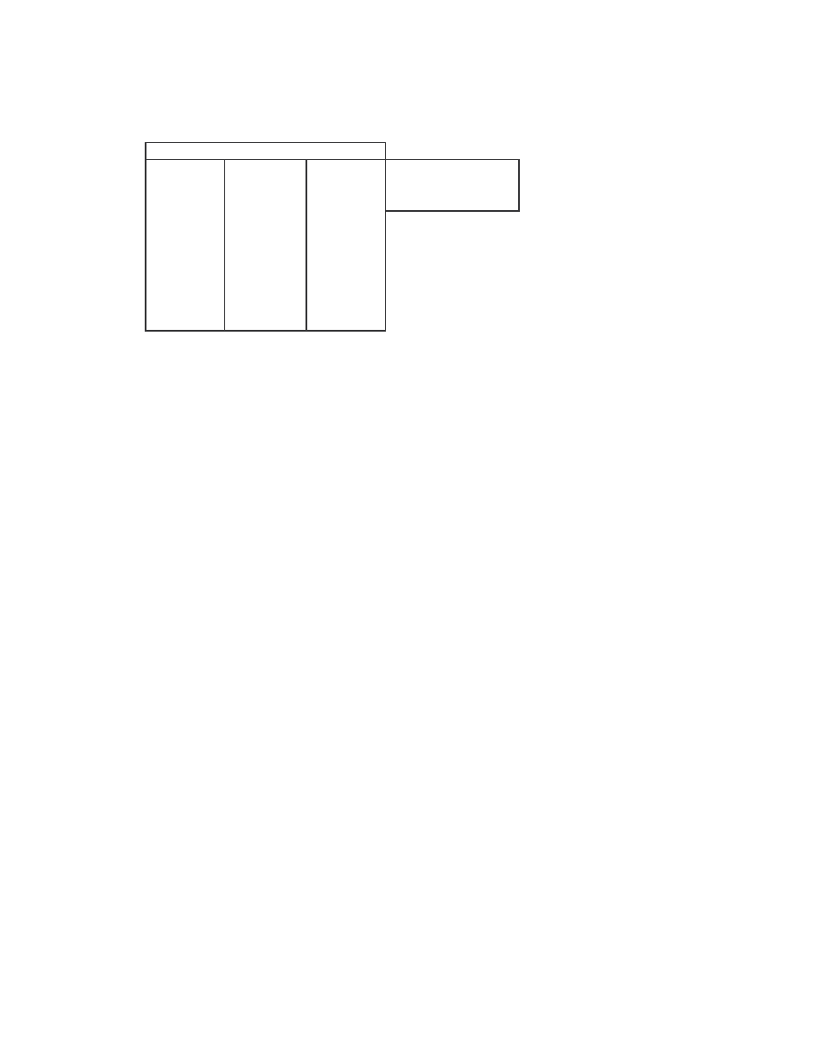
79
Table A-4 Similarity scores between MPCGEN virus variants.
Similarity scores between files:
IDA_MPC0 IDA_MPC1
0.45032
min
0.44964
IDA_MPC0 IDA_MPC2
0.46885
max
0.96568
IDA_MPC0 IDA_MPC3
0.78035 average
0.62704
IDA_MPC0 IDA_MPC4
0.44970
IDA_MPC1 IDA_MPC2
0.80875
IDA_MPC1 IDA_MPC3
0.57993
IDA_MPC1 IDA_MPC4
0.96568
IDA_MPC2 IDA_MPC3
0.44964
IDA_MPC2 IDA_MPC4
0.80704
IDA_MPC3 IDA_MPC4
0.51009
80
Table A-5 Similarity scores between random normal files.
IDA_R0 IDA_R1 0.35683 IDA_R3 IDA_R13 0.33470 IDA_R8 IDA_R11 0.18961
min
0.14369
IDA_R0 IDA_R2 0.50040 IDA_R3 IDA_R14 0.23842 IDA_R8 IDA_R12 0.23820
max
0.72535
IDA_R0 IDA_R3 0.33053 IDA_R3 IDA_R15 0.35729 IDA_R8 IDA_R13 0.15451 average 0.36337
IDA_R0 IDA_R4 0.37981 IDA_R3 IDA_R16 0.44687 IDA_R8 IDA_R14 0.14006
IDA_R0 IDA_R5 0.19924 IDA_R3 IDA_R17 0.37535 IDA_R8 IDA_R15 0.20801
IDA_R0 IDA_R6 0.19600 IDA_R3 IDA_R18 0.42995 IDA_R8 IDA_R16 0.27208
IDA_R0 IDA_R7 0.19905 IDA_R3 IDA_R19 0.27338 IDA_R8 IDA_R17 0.22085
IDA_R0 IDA_R8 0.19984 IDA_R4 IDA_R5 0.18656 IDA_R8 IDA_R18 0.24303
IDA_R0 IDA_R9 0.33228 IDA_R4 IDA_R6 0.17777 IDA_R8 IDA_R19 0.15206
IDA_R0 IDA_R10 0.49773 IDA_R4 IDA_R7 0.18059 IDA_R9 IDA_R10 0.49678
IDA_R0 IDA_R11 0.41739 IDA_R4 IDA_R8 0.18726 IDA_R9 IDA_R11 0.30930
IDA_R0 IDA_R12 0.38726 IDA_R4 IDA_R9 0.37206 IDA_R9 IDA_R12 0.27024
IDA_R0 IDA_R13 0.29789 IDA_R4 IDA_R10 0.51310 IDA_R9 IDA_R13 0.34013
IDA_R0 IDA_R14 0.31944 IDA_R4 IDA_R11 0.34440 IDA_R9 IDA_R14 0.25781
IDA_R0 IDA_R15 0.46465 IDA_R4 IDA_R12 0.36972 IDA_R9 IDA_R15 0.38430
IDA_R0 IDA_R16 0.48780 IDA_R4 IDA_R13 0.36090 IDA_R9 IDA_R16 0.44825
IDA_R0 IDA_R17 0.41608 IDA_R4 IDA_R14 0.25833 IDA_R9 IDA_R17 0.41396
IDA_R0 IDA_R18 0.39995 IDA_R4 IDA_R15 0.39103 IDA_R9 IDA_R18 0.36174
IDA_R0 IDA_R19 0.34073 IDA_R4 IDA_R16 0.48730 IDA_R9 IDA_R19 0.28417
IDA_R1 IDA_R2 0.45579 IDA_R4 IDA_R17 0.42200 IDA_R10 IDA_R11 0.45079
IDA_R1 IDA_R3 0.29938 IDA_R4 IDA_R18 0.44600 IDA_R10 IDA_R12 0.45866
IDA_R1 IDA_R4 0.35691 IDA_R4 IDA_R19 0.30770 IDA_R10 IDA_R13 0.44319
IDA_R1 IDA_R5 0.17400 IDA_R5 IDA_R6 0.89691 IDA_R10 IDA_R14 0.35968
IDA_R1 IDA_R6 0.17063 IDA_R5 IDA_R7 0.91066 IDA_R10 IDA_R15 0.49985
IDA_R1 IDA_R7 0.17639 IDA_R5 IDA_R8 0.93395 IDA_R10 IDA_R16 0.65204
IDA_R1 IDA_R8 0.17465 IDA_R5 IDA_R9 0.16720 IDA_R10 IDA_R17 0.52560
IDA_R1 IDA_R9 0.24162 IDA_R5 IDA_R10 0.26957 IDA_R10 IDA_R18 0.51452
IDA_R1 IDA_R10 0.40046 IDA_R5 IDA_R11 0.18895 IDA_R10 IDA_R19 0.40760
IDA_R1 IDA_R11 0.43216 IDA_R5 IDA_R12 0.23733 IDA_R11 IDA_R12 0.36396
IDA_R1 IDA_R12 0.67496 IDA_R5 IDA_R13 0.15394 IDA_R11 IDA_R13 0.31181
IDA_R1 IDA_R13 0.24293 IDA_R5 IDA_R14 0.13945 IDA_R11 IDA_R14 0.29316
IDA_R1 IDA_R14 0.26337 IDA_R5 IDA_R15 0.20742 IDA_R11 IDA_R15 0.51267
IDA_R1 IDA_R15 0.45401 IDA_R5 IDA_R16 0.27140 IDA_R11 IDA_R16 0.45261
IDA_R1 IDA_R16 0.40808 IDA_R5 IDA_R17 0.22024 IDA_R11 IDA_R17 0.36685
IDA_R1 IDA_R17 0.34480 IDA_R5 IDA_R18 0.24225 IDA_R11 IDA_R18 0.41693
IDA_R1 IDA_R18 0.41433 IDA_R5 IDA_R19 0.15141 IDA_R11 IDA_R19 0.30487
IDA_R1 IDA_R19 0.27158 IDA_R6 IDA_R7 0.88308 IDA_R12 IDA_R13 0.27602
IDA_R2 IDA_R3 0.48679 IDA_R6 IDA_R8 0.89003 IDA_R12 IDA_R14 0.28409
IDA_R2 IDA_R4 0.54079 IDA_R6 IDA_R9 0.16231 IDA_R12 IDA_R15 0.38460
IDA_R2 IDA_R5 0.27792 IDA_R6 IDA_R10 0.26633 IDA_R12 IDA_R16 0.45005
IDA_R2 IDA_R6 0.27305 IDA_R6 IDA_R11 0.18593 IDA_R12 IDA_R17 0.36188
IDA_R2 IDA_R7 0.27697 IDA_R6 IDA_R12 0.23077 IDA_R12 IDA_R18 0.43837
IDA_R2 IDA_R8 0.27855 IDA_R6 IDA_R13 0.13848 IDA_R12 IDA_R19 0.30907
IDA_R2 IDA_R9 0.47721 IDA_R6 IDA_R14 0.13603 IDA_R13 IDA_R14 0.25747
IDA_R2 IDA_R10 0.72404 IDA_R6 IDA_R15 0.20427 IDA_R13 IDA_R15 0.37897
IDA_R2 IDA_R11 0.45543 IDA_R6 IDA_R16 0.26421 IDA_R13 IDA_R16 0.41097
IDA_R2 IDA_R12 0.49804 IDA_R6 IDA_R17 0.20671 IDA_R13 IDA_R17 0.42617
IDA_R2 IDA_R13 0.47001 IDA_R6 IDA_R18 0.23949 IDA_R13 IDA_R18 0.39149
IDA_R2 IDA_R14 0.32956 IDA_R6 IDA_R19 0.14545 IDA_R13 IDA_R19 0.27386
IDA_R2 IDA_R15 0.53073 IDA_R7 IDA_R8 0.90905 IDA_R14 IDA_R15 0.34984
IDA_R2 IDA_R16 0.72535 IDA_R7 IDA_R9 0.16587 IDA_R14 IDA_R16 0.31725
IDA_R2 IDA_R17 0.51154 IDA_R7 IDA_R10 0.27080 IDA_R14 IDA_R17 0.32478
IDA_R2 IDA_R18 0.53837 IDA_R7 IDA_R11 0.18709 IDA_R14 IDA_R18 0.27324
IDA_R2 IDA_R19 0.40102 IDA_R7 IDA_R12 0.23494 IDA_R14 IDA_R19 0.24026
IDA_R3 IDA_R4 0.45359 IDA_R7 IDA_R13 0.14106 IDA_R15 IDA_R16 0.54225
IDA_R3 IDA_R5 0.14913 IDA_R7 IDA_R14 0.13775 IDA_R15 IDA_R17 0.40120
IDA_R3 IDA_R6 0.14369 IDA_R7 IDA_R15 0.20724 IDA_R15 IDA_R18 0.46115
IDA_R3 IDA_R7 0.14617 IDA_R7 IDA_R16 0.26824 IDA_R15 IDA_R19 0.36554
IDA_R3 IDA_R8 0.15209 IDA_R7 IDA_R17 0.20990 IDA_R16 IDA_R17 0.47555
IDA_R3 IDA_R9 0.32238 IDA_R7 IDA_R18 0.23978 IDA_R16 IDA_R18 0.51024
IDA_R3 IDA_R10 0.44973 IDA_R7 IDA_R19 0.14865 IDA_R16 IDA_R19 0.36608
IDA_R3 IDA_R11 0.28466 IDA_R8 IDA_R9 0.16777 IDA_R17 IDA_R18 0.44026
IDA_R3 IDA_R12 0.31646 IDA_R8 IDA_R10 0.27017 IDA_R17 IDA_R19 0.31786
IDA_R18 IDA_R19 0.30629
Similarity scores between files:
81
Table A-6 Similarity scores between NGVCK virus and VCL32 virus pairs that
have score greater than 0.
Similarity scores between files:
IDA_NGVCK0 IDA_VCL0
0.04240
min
0.01192
IDA_NGVCK0 IDA_VCL1
0.04980
max
0.05517
IDA_NGVCK0 IDA_VCL2
0.03285 average
0.02477
IDA_NGVCK0 IDA_VCL3
0.03569
IDA_NGVCK0 IDA_VCL4
0.05517
IDA_NGVCK0 IDA_VCL5
0.03101
IDA_NGVCK0 IDA_VCL6
0.04150
IDA_NGVCK0 IDA_VCL7
0.04240
IDA_NGVCK0 IDA_VCL8
0.04362
IDA_NGVCK0 IDA_VCL9
0.04312
IDA_NGVCK1 IDA_VCL0
0.01552
IDA_NGVCK1 IDA_VCL1
0.01785
IDA_NGVCK1 IDA_VCL2
0.01250
IDA_NGVCK1 IDA_VCL3
0.01340
IDA_NGVCK1 IDA_VCL4
0.01955
IDA_NGVCK1 IDA_VCL5
0.01192
IDA_NGVCK1 IDA_VCL6
0.01523
IDA_NGVCK1 IDA_VCL7
0.01552
IDA_NGVCK1 IDA_VCL8
0.01590
IDA_NGVCK1 IDA_VCL9
0.01574
IDA_NGVCK2 IDA_VCL2
0.01265
IDA_NGVCK2 IDA_VCL3
0.01354
IDA_NGVCK2 IDA_VCL5
0.01207
IDA_NGVCK5 IDA_VCL0
0.01558
IDA_NGVCK5 IDA_VCL1
0.01792
IDA_NGVCK5 IDA_VCL2
0.01257
IDA_NGVCK5 IDA_VCL3
0.01346
IDA_NGVCK5 IDA_VCL4
0.01961
IDA_NGVCK5 IDA_VCL5
0.01198
IDA_NGVCK5 IDA_VCL6
0.01530
IDA_NGVCK5 IDA_VCL7
0.01558
IDA_NGVCK5 IDA_VCL8
0.01597
IDA_NGVCK5 IDA_VCL9
0.01581
IDA_NGVCK9 IDA_VCL0
0.02653
IDA_NGVCK9 IDA_VCL1
0.03120
IDA_NGVCK9 IDA_VCL2
0.03409
IDA_NGVCK9 IDA_VCL3
0.03678
IDA_NGVCK9 IDA_VCL4
0.03459
IDA_NGVCK9 IDA_VCL5
0.03235
IDA_NGVCK9 IDA_VCL6
0.02596
IDA_NGVCK9 IDA_VCL7
0.02653
IDA_NGVCK9 IDA_VCL8
0.02729
IDA_NGVCK9 IDA_VCL9
0.02698
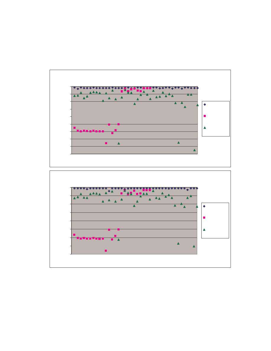
82
Appendix B: HMM training and testing results
Table B-1 Log likelihood per opcode (LLPO) of family viruses, non-family viruses
and normal files with N = 3.
Test set 0, N = 3
-180
-160
-140
-120
-100
-80
-60
-40
-20
0
0
10
20
30
40
File number
S
co
re
(
L
L
P
O
)
test set 0
non-family
viruses
normal files
Test set 1, N = 3
-160
-140
-120
-100
-80
-60
-40
-20
0
0
10
20
30
40
File number
S
co
re
(L
LP
O
)
test set 1
non-family
viruses
normal files
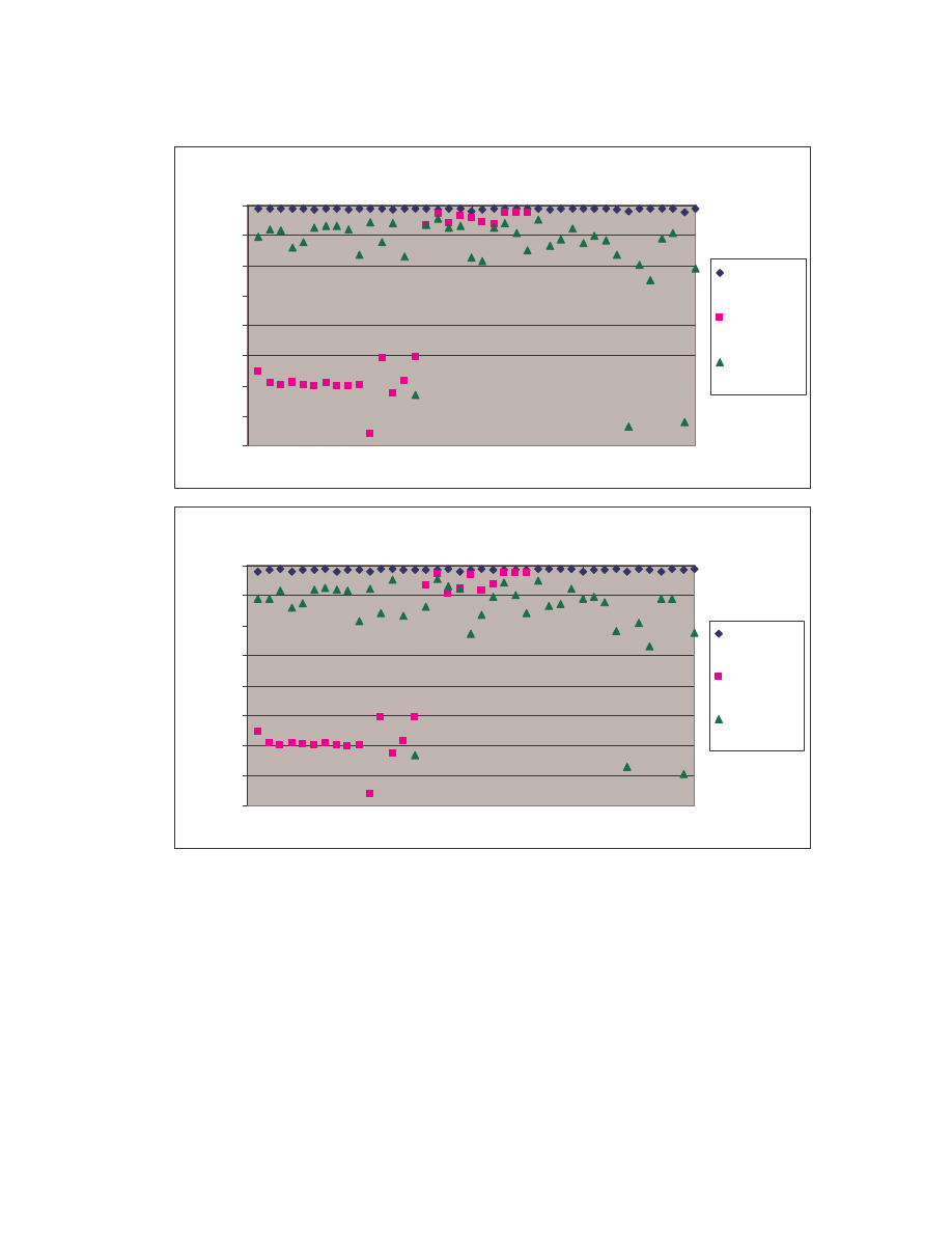
83
Test set 2, N = 3
-160
-140
-120
-100
-80
-60
-40
-20
0
0
10
20
30
40
File number
S
co
re
(
L
L
P
O
)
test set 2
non-family
viruses
normal files
Test set 3, N = 3
-160
-140
-120
-100
-80
-60
-40
-20
0
0
10
20
30
40
File number
S
co
re
(
L
L
P
O
)
test set 3
non-family
viruses
normal files
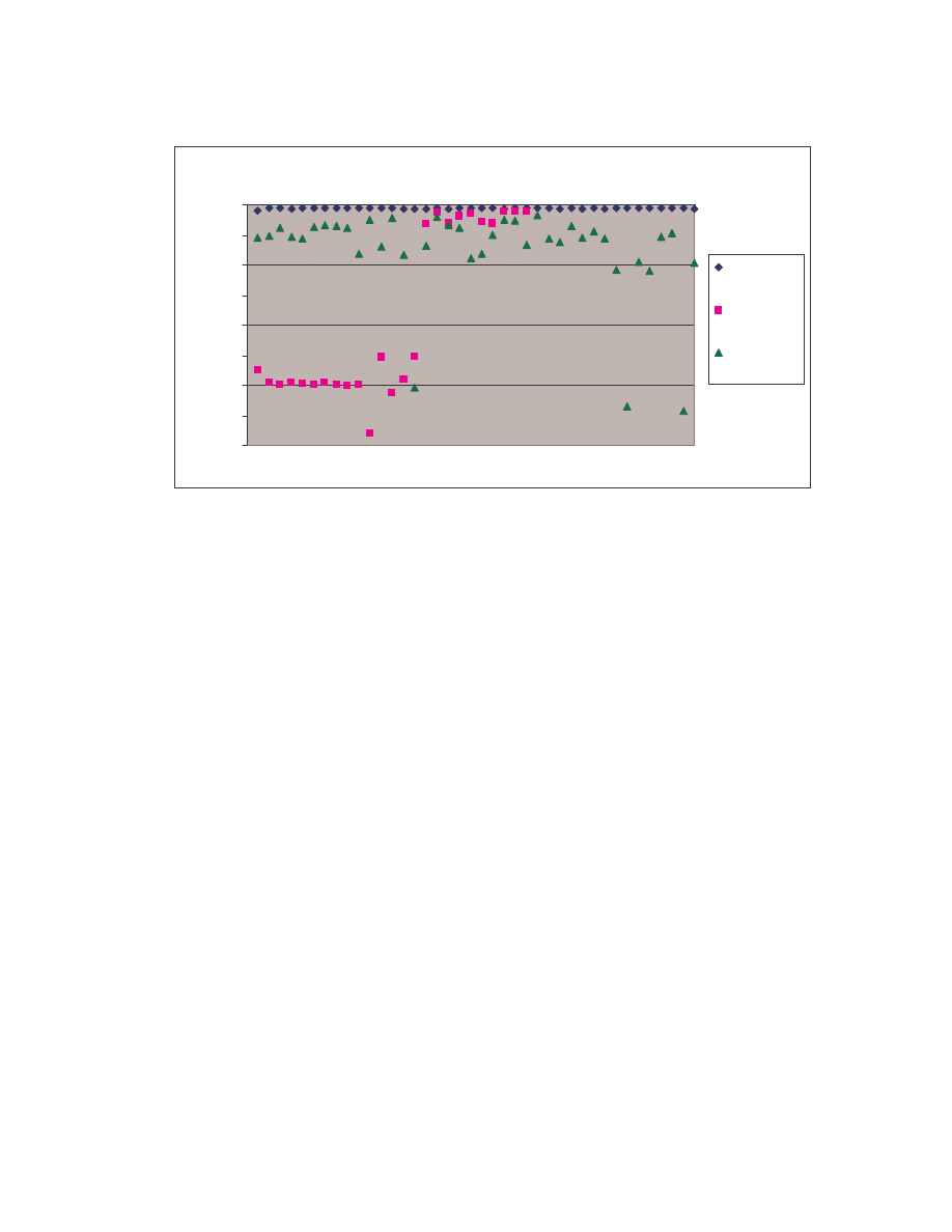
84
Test set 4, N = 3
-160
-140
-120
-100
-80
-60
-40
-20
0
0
10
20
30
40
File number
S
co
re
(
L
L
P
O
)
test set 4
non-family
viruses
normal files
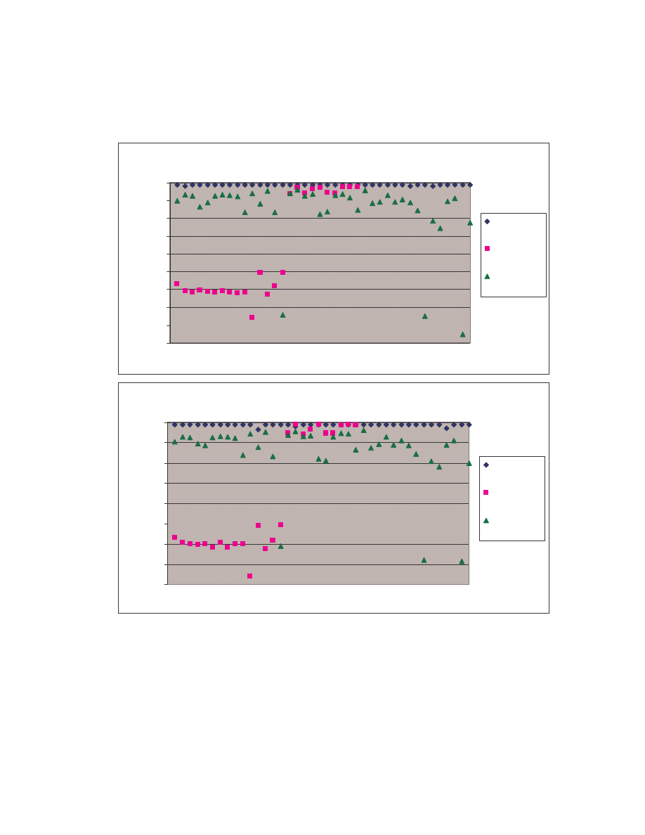
85
Table B-2 Log likelihood per opcode (LLPO) of family viruses, non-family viruses
and normal files with N = 5.
Test set 0, N = 5
-180
-160
-140
-120
-100
-80
-60
-40
-20
0
0
10
20
30
40
File number
S
co
re
(
L
L
P
O
)
test set 0
non-family
viruses
normal files
Test set 1, N = 5
-160
-140
-120
-100
-80
-60
-40
-20
0
0
10
20
30
40
File number
S
co
re
(
L
L
P
O
)
test set 1
non-family
viruses
normal files
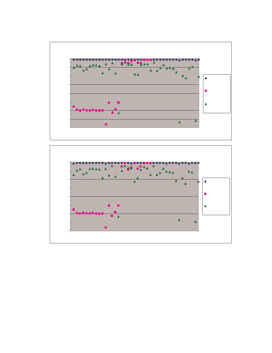
86
Test set 2, N = 5
-160
-140
-120
-100
-80
-60
-40
-20
0
0
10
20
30
40
File number
S
co
re
(
L
L
P
O
)
test set 2
non-family
viruses
normal files
Test set 3, N = 5
-160
-140
-120
-100
-80
-60
-40
-20
0
0
10
20
30
40
File number
S
co
re
(
L
L
P
O
)
test set 3
non-family
viruses
normal files

87
Test set 4, N = 5
-160
-140
-120
-100
-80
-60
-40
-20
0
0
10
20
30
40
File number
S
co
re
(
L
L
P
O
)
test set 4
non-family
viruses
normal files
88
Table B-3 Raw LLPO scores of all 105 programs returned by the 25 HMMs. The
scores are grouped according to the test set used by an HMM. For each test set, 5
models with N = 2 to 6 were tested.
Test set 0
N = 2
N = 3
N = 4
N = 5
N = 6
Test set 1
N = 2
N = 3
N = 4
N = 5
N = 6
Files in the test set (same family viruses):
Files in the test set (same family viruses):
IDA_N0
-2.83844 -2.69903
-2.6256 -2.60804 -2.52266 IDA_N40
-2.76366 -2.68011 -2.58964 -2.53576 -2.51455
IDA_N1
-4.38048 -5.85754 -4.19275
-4.1669 -4.06707 IDA_N41
-2.66436 -2.58935
-2.5111 -2.47107 -2.45238
IDA_N2
-2.85605
-2.7188 -2.68132 -2.67629 -2.55774 IDA_N42
-2.69348 -2.61696 -2.52229
-2.4727
-2.4123
IDA_N3
-2.68468 -4.33065 -2.49798 -2.47691 -2.39205 IDA_N43
-2.67667 -2.65022 -2.53879 -2.47592 -2.48122
IDA_N4
-2.78905 -4.34511 -2.58534 -2.55277 -2.47677 IDA_N44
-2.81877 -4.30004 -2.66655 -2.60316 -4.10904
IDA_N5
-2.87672 -4.34558 -2.65451 -2.64242 -2.55389 IDA_N45
-2.71112 -2.64813 -2.57352 -2.51464 -4.11693
IDA_N6
-2.79097 -2.65019 -2.62367 -2.61525 -2.48092 IDA_N46
-2.68092 -2.61321 -2.51652 -2.42621 -2.42194
IDA_N7
-2.692 -4.34712
-2.4885 -2.47446 -2.39059 IDA_N47
-2.69872 -2.61577 -2.52154 -2.45126 -2.42594
IDA_N8
-2.82293 -4.45772 -2.65826 -2.63877 -2.52677 IDA_N48
-2.83159
-2.7425 -2.67465 -2.60111 -2.58626
IDA_N9
-2.71437 -4.45754 -2.52941 -2.51297 -2.42621 IDA_N49
-2.6207
-2.5232 -2.42938 -2.37143
-2.366
IDA_N10
-2.77855 -4.31873 -2.56441 -2.53805 -2.42304 IDA_N50
-2.61617 -2.55355 -2.46196 -2.41996
-2.3982
IDA_N11
-2.68199 -4.44285 -2.47388 -2.44936 -2.35678 IDA_N51
-7.58719 -9.03848 -7.40715
-7.3438 -8.87874
IDA_N12
-2.85616
-2.7279 -2.65932 -2.65164 -2.55999 IDA_N52
-2.64667
-2.5732 -2.47363
-2.4236 -2.41241
IDA_N13
-2.73863 -4.41354 -2.53999 -2.50189 -2.38622 IDA_N53
-2.61651 -2.54794
-2.4426 -2.36823 -2.33674
IDA_N14
-2.77855 -4.29042 -2.57118 -2.55275 -2.45347 IDA_N54
-2.73205 -2.66418 -2.57222 -2.50114 -2.48516
IDA_N15
-2.81468 -4.35899 -2.56416 -2.55566 -2.47357 IDA_N55
-2.73317 -2.64225 -2.55513 -2.47167
-2.4622
IDA_N16
-2.74838 -2.63712 -2.56975 -2.56795 -2.46139 IDA_N56
-4.48225 -4.43088 -4.32367 -4.24991 -5.90228
IDA_N17
-2.76431 -2.62497 -2.58408 -2.56227 -2.46164 IDA_N57
-2.91714 -2.86797 -2.76512 -2.70085 -2.69654
IDA_N18
-2.77806 -4.51851 -2.60557 -2.58518
-2.4591 IDA_N58
-2.70093 -2.63116 -2.54547 -2.48439 -2.46275
IDA_N19
-2.79064 -4.45237 -2.58552 -2.57452 -2.50117 IDA_N59
-2.73989 -2.68482 -2.55744
-2.5066 -2.49595
IDA_N20
-2.82825 -2.68674 -2.65981 -2.64895 -2.48132 IDA_N60
-2.70015
-2.6004
-2.5185 -2.46014 -2.41017
IDA_N21
-2.71906 -2.55134 -2.49386 -2.48976 -2.37984 IDA_N61
-2.6528 -2.60145 -2.51327
-2.4788 -2.43913
IDA_N22
-2.85215 -4.38385 -2.64538 -2.62988 -2.52194 IDA_N62
-2.68543 -2.59348 -2.49426
-2.4262 -2.45459
IDA_N23
-2.79084 -4.44067
-2.5707 -2.54889 -2.46194 IDA_N63
-2.76852 -2.72129 -2.62608 -2.55203 -2.55381
IDA_N24
-2.74196 -2.58964 -2.57811 -2.54555 -2.43279 IDA_N64
-2.65427 -2.57621 -2.48448 -2.41291 -2.43595
IDA_N25
-2.83737 -2.69987 -2.65412 -2.64446 -2.51287 IDA_N65
-2.75828 -2.65424
-2.5927 -2.51481 -2.51811
IDA_N26
-2.75602 -2.59864
-2.5706 -2.55371 -2.45323 IDA_N66
-2.82538 -2.72391 -2.62952 -2.56258 -2.57424
IDA_N27
-2.74015 -4.48543 -2.57684 -2.55921 -2.44652 IDA_N67
-2.78551 -2.70432 -2.61095 -2.55111
-2.5417
IDA_N28
-2.79382 -4.31769 -2.61515 -2.59072 -2.46932 IDA_N68
-2.61916 -2.52407 -2.41714 -2.35491
-2.3518
IDA_N29
-2.81342 -2.65369 -2.59382 -2.58248 -2.46846 IDA_N69
-2.71171
-2.6363 -2.53841 -2.48086 -2.45506
IDA_N30
-2.90366 -2.76041 -2.71772 -2.69408 -2.59481 IDA_N70
-2.78421 -2.78217 -2.63006 -2.57823 -4.15636
IDA_N31
-4.43492 -5.78653
-4.2053 -4.17633 -4.08559 IDA_N71
-2.78259 -2.74365 -2.61111 -2.56922 -2.57302
IDA_N32
-2.78984 -2.65151 -2.60353 -2.57938 -2.51671 IDA_N72
-2.76467
-2.675 -2.58198 -2.51358 -2.50767
IDA_N33
-2.71116 -2.54243 -2.49379 -2.48103 -2.35476 IDA_N73
-2.81895 -2.73003
-2.6272 -2.55822 -2.57578
IDA_N34
-4.40097 -5.77089
-4.1931
-4.183 -4.07268 IDA_N74
-2.73572 -2.64437 -2.54353 -2.48121 -2.46222
IDA_N35
-2.83606 -2.69768 -2.64939 -2.63737 -2.53085 IDA_N75
-2.77316 -2.69325 -2.58006 -2.54218 -2.50283
IDA_N36
-2.80357
-2.6256 -2.59359 -2.56195 -2.45723 IDA_N76
-6.072
-5.9712 -5.92025 -5.83644 -5.85622
IDA_N37
-2.80591 -4.37577 -2.61369 -2.59847 -2.48674 IDA_N77
-2.71058 -2.66658 -2.54104 -2.47233 -2.44444
IDA_N38
-2.93256 -4.36418 -2.75564 -2.74424
-2.6344 IDA_N78
-2.63596 -2.56586
-2.4402 -2.42373
-2.3633
IDA_N39
-2.7216
-4.3746 -2.50902
-2.4919 -2.37628 IDA_N79
-2.80304
-2.7073 -2.60189 -2.55057 -4.15786
min LLPO
-4.43492 -5.85754
-4.2053
-4.183 -4.08559 min LLPO -7.58719 -9.03848 -7.40715
-7.3438 -8.87874

89
Test set 0
N = 2
N = 3
N = 4
N = 5
N = 6
Test set 1
N = 2
N = 3
N = 4
N = 5
N = 6
Files in the comparison set (other non-family viruses):
Files in the comparison set (other non-family viruses):
IDA_V0
-110.68 -110.537
-110.51 -113.672
-116.88 IDA_V0
-110.536 -113.711 -110.501 -113.692 -116.841
IDA_V1
-118.423 -118.391 -118.353
-121.55 -121.655 IDA_V1
-118.371 -121.604 -118.343 -118.388 -124.765
IDA_V2
-120.033 -119.994 -119.985
-123.12 -126.317 IDA_V2
-119.985 -123.157
-119.95 -120.005 -126.302
IDA_V3
-118.026 -117.894 -117.861 -121.052
-124.29 IDA_V3
-117.886 -121.094 -117.853 -121.068 -124.252
IDA_V4
-119.478 -119.441 -119.435 -122.557 -122.634 IDA_V4
-119.443 -122.598 -119.408 -119.468 -125.714
IDA_V5
-120.159 -120.023 -120.001 -123.151 -126.352 IDA_V5
-120.012 -123.186
-119.98 -123.182 -126.339
IDA_V6
-118.432 -118.405 -118.378 -121.564
-124.82 IDA_V6
-118.4 -121.625 -118.366 -118.397 -124.793
IDA_V7
-120.167 -120.034
-120.01 -123.166 -126.374 IDA_V7
-120.036 -123.211
-120 -123.186 -126.336
IDA_V8
-120.567 -120.541 -120.526 -123.673 -126.889 IDA_V8
-120.521 -123.716
-120.49 -120.543 -126.868
IDA_V9
-120.013 -119.976 -119.965
-123.1 -123.188 IDA_V9
-119.976 -123.149 -119.941 -120.001 -126.283
IDA_V10
-152.12
-152.01 -152.124 -152.131 -151.978 IDA_V10
-152.129 -152.073 -152.036 -151.955 -152.017
IDA_V11
-101.51 -101.422 -101.479 -101.473 -101.482 IDA_V11
-101.476 -101.458 -101.353
-101.4 -101.429
IDA_V12
-125.284 -125.185 -125.229 -125.227
-125.14 IDA_V12
-125.255 -125.203 -125.129 -125.125 -125.186
IDA_V13
-116.654 -116.559 -116.657 -116.667 -116.685 IDA_V13
-116.641 -116.635
-116.55 -116.564 -116.599
IDA_V14
-101.059 -100.975 -101.033
-101.03 -101.034 IDA_V14
-101.031
-101.01 -100.905 -100.953 -100.978
IDA_V15
-11.0989 -12.9583 -12.9958 -12.9572 -12.8483 IDA_V15
-11.0055 -15.0036 -12.8509 -10.8721 -14.8833
IDA_V16
-2.99929 -5.40678 -5.37187 -5.33721 -5.30616 IDA_V16
-2.86441 -7.99111 -5.24582 -2.67224 -7.76235
IDA_V17
-10.9101 -12.1256 -12.1616 -12.1392
-13.36 IDA_V17
-12.1081 -17.4324 -13.2475 -12.0539 -17.2344
IDA_V18
-6.07548 -7.51274 -7.50533 -7.48802 -8.96855 IDA_V18
-7.45631 -13.6628 -8.80031
-7.3797 -13.3882
IDA_V19
-2.95565 -5.73581 -5.74302 -5.68135 -5.61087 IDA_V19
-2.82419
-8.7245 -5.60009
-2.6033 -8.64268
IDA_V20
-10.1124 -11.1703
-11.21 -11.1938 -12.2449 IDA_V20
-11.1813 -15.9209 -10.9923 -11.0869 -14.5662
IDA_V21
-10.8532 -12.6338 -12.6657 -12.6302
-14.45 IDA_V21
-10.7554 -14.6156 -12.5222 -10.6257 -14.4848
IDA_V22
-3.06677 -4.89731
-4.8795 -4.86404 -6.75131 IDA_V22
-2.94324 -6.93559 -2.72727 -2.72782 -4.72337
IDA_V23
-3.04203 -4.96946 -4.94235 -4.92553 -4.82566 IDA_V23
-2.91692 -7.09299 -2.70189 -2.68671 -4.77661
IDA_V24
-3.0499 -4.94289
-4.941
-4.9183 -4.81091 IDA_V24
-2.93749 -7.02483
-2.7352 -2.70715 -4.78438
max LLPO
-2.95565 -4.89731
-4.8795 -4.86404 -4.81091 max LLPO -2.82419 -6.93559 -2.70189
-2.6033 -4.72337
Files in the comparison set (normal files):
Files in the comparison set (normal files):
IDA_R0
-20.3522 -24.4795 -20.1793 -20.1959 -25.7882 IDA_R0
-19.0813 -25.6181 -25.4629 -19.3923
-30.964
IDA_R1
-13.9877 -24.3116 -14.7271 -13.9233
-24.204 IDA_R1
-12.9742 -23.3083 -25.8326 -14.1531 -33.5984
IDA_R2
-14.9357 -16.5983 -14.8663 -14.9016 -15.7212 IDA_R2
-14.892 -15.7651 -17.3202 -14.9418 -18.2097
IDA_R3
-27.6756 -31.0684
-27.647 -27.6873 -31.0792 IDA_R3
-20.9218 -24.3491 -27.5827 -21.1412 -32.0876
IDA_R4
-22.7756 -25.8777 -22.7729 -22.8071 -25.8243 IDA_R4
-22.7361 -25.2426 -26.9897 -22.9385 -32.4967
IDA_R5
-15.1323 -16.2721 -15.0734
-15.113 -15.5831 IDA_R5
-15.0357 -15.6858 -18.4092 -15.1611 -22.9879
IDA_R6
-13.7367 -14.7423 -13.6801 -13.7221 -14.1334 IDA_R6
-13.6455 -14.2019
-17.131 -13.7405 -21.7219
IDA_R7
-14.1954 -15.2444 -14.1447 -14.1902 -14.5943 IDA_R7
-14.1103 -14.6935 -17.2122 -14.7183 -21.4581
IDA_R8
-15.8122 -16.9595 -15.7393 -15.7798 -16.2559 IDA_R8
-15.7075 -16.3599
-19.681 -15.8273 -24.2979
IDA_R9
-33.7738 -37.8438 -33.7409 -33.7792 -37.8095 IDA_R9
-32.1023 -33.8338 -36.1359 -32.3185 -45.0598
IDA_R10
-12.2689 -17.6877 -12.2309
-12.267 -16.6443 IDA_R10
-10.0797 -13.3747 -14.3734 -11.3154 -19.7933
IDA_R11
-23.8743 -30.9366 -23.7247 -23.7407 -30.8355 IDA_R11
-23.7319 -30.9349 -30.8593 -24.5349
-37.361
IDA_R12
-9.48983 -10.4038 -10.3103 -9.50058 -10.3326 IDA_R12
-8.59588 -9.53152 -17.9652 -9.67963
-18.9
IDA_R13
-33.6615 -33.7398 -33.6666 -33.7372 -33.6222 IDA_R13
-33.5891 -33.6865 -38.6692 -33.8411 -38.7489
IDA_R14
-148.522 -152.084 -148.487 -148.489 -153.152 IDA_R14
-120.268 -124.967 -125.499 -122.262 -137.027
IDA_R15
-12.2724 -28.6864 -12.0183 -12.0659 -29.7013 IDA_R15
-11.9631 -28.6641 -26.4973 -12.3387 -38.9709
IDA_R16
-8.06632 -8.90711 -7.99737 -8.02997 -8.03371 IDA_R16
-8.01384 -8.08398
-14.426 -8.97044 -16.1008
IDA_R17
-14.7949 -16.0352 -14.7868 -14.8274 -18.3719 IDA_R17
-13.5173 -13.5915 -15.8967 -13.6832 -20.7959
IDA_R18
-13.0679 -16.4832 -12.9911 -13.0175 -15.7305 IDA_R18
-12.9705 -15.7858
-16.37 -13.0381 -18.5487
IDA_R19
-35.6981 -46.1659 -35.6743 -35.6973 -46.0777 IDA_R19
-34.6171 -44.0611 -36.6797 -35.8427 -46.6268
IDA_R20
-33.1515 -33.8698 -35.4995 -33.0993 -35.4245 IDA_R20
-33.0387
-33.851 -36.1835 -37.9465 -37.0886
IDA_R21
-14.2326
-21.767
-14.113 -14.1297 -21.7071 IDA_R21
-14.0953 -21.7596 -20.9419 -14.2059 -28.6001
IDA_R22
-12.9223 -13.8657 -12.8723
-12.895 -14.7197 IDA_R22
-9.95689 -15.2951 -21.6112 -10.9678 -31.1503
IDA_R23
-16.9245 -21.3879
-17.77 -16.9387
-21.244 IDA_R23
-10.6694 -15.2433 -17.7176 -11.7232 -22.1688
IDA_R24
-30.9469 -32.7376 -30.8959 -30.9188 -33.5087 IDA_R24
-26.6315 -28.5351 -42.8449 -27.3516 -47.9732
IDA_R25
-9.16703 -10.7777 -9.04651 -9.05832 -10.2173 IDA_R25
-7.38424 -8.57564 -9.57934 -7.98664 -11.9263
IDA_R26
-22.6304 -28.2234 -27.2185 -23.3968
-35.911 IDA_R26
-19.4715 -25.3171
-30.06 -25.4243 -34.9636
IDA_R27
-21.8092 -26.9106 -21.7096
-21.747 -26.8393 IDA_R27
-21.694 -26.8971 -28.5276 -21.8715
-34.6
IDA_R28
-14.3619 -15.5332 -14.3302
-14.359 -14.2727 IDA_R28
-14.2948
-14.356 -21.1883 -14.3848 -23.5694
IDA_R29
-22.0801 -25.3197 -21.9719 -22.0301
-22.023 IDA_R29
-21.9533 -22.0916 -28.2818 -22.1719
-28.228
IDA_R30
-19.172 -20.1903 -19.1305 -19.1455 -21.1287 IDA_R30
-18.087
-18.151 -24.0749 -18.2444 -25.1344
IDA_R31
-22.5469 -24.8483 -22.5491 -22.5927 -24.7886 IDA_R31
-22.5222 -24.8293 -24.7074 -22.6012 -29.2088
IDA_R32
-31.503 -43.6435 -31.2799 -31.3329 -43.5575 IDA_R32
-31.215 -43.6288
-47.021 -31.3551 -48.8613
IDA_R33
-149.001 -149.753 -149.077 -149.735
-149.66 IDA_R33
-134.309 -134.301 -135.629 -135.861 -135.683
IDA_R34
-42.8888 -43.5834 -42.7889 -42.8023
-43.542 IDA_R34
-37.7545 -39.0629 -42.0903 -38.5235 -45.3049
IDA_R35
-51.267 -54.4469
-51.2 -51.2107 -54.3881 IDA_R35
-43.5655 -46.8861 -57.5935 -43.7333 -61.4655
IDA_R36
-21.458 -21.5564 -21.4072 -21.4287 -24.0999 IDA_R36
-21.3869 -24.9779 -29.0406 -22.4636 -40.1465
IDA_R37
-17.9681 -21.4674 -17.7994 -17.8171 -23.2231 IDA_R37
-17.8202 -20.6498 -23.1537 -18.2312 -33.7685
IDA_R38
-169.192 -169.933
-169.2 -170.533 -171.988 IDA_R38
-136.402 -141.157
-140.4 -137.329
-146.51
IDA_R39
-45.4978 -49.2993 -45.4443 -45.4541 -52.5257 IDA_R39
-38.6277 -45.6849 -51.1963 -40.0192 -62.7995
max LLPO
-8.06632 -8.90711 -7.99737 -8.02997 -8.03371 max LLPO -7.38424 -8.08398 -9.57934 -7.98664 -11.9263

90
Test set 2
N = 2
N = 3
N = 4
N = 5
N = 6
Test set 3
N = 2
N = 3
N = 4
N = 5
N = 6
Files in the test set (same family viruses):
Files in the test set (same family viruses):
IDA_N80
-2.78596 -2.67798 -2.59714 -2.54315 -2.50417 IDA_N120
-4.40838
-4.3549 -4.24551 -4.21035 -4.16695
IDA_N81
-2.71582 -2.61435 -2.51226
-2.483 -2.44984 IDA_N121
-2.79207
-2.762 -2.64508 -2.62348 -2.58086
IDA_N82
-2.74543 -2.65419 -2.56718 -2.51449 -2.51249 IDA_N122
-2.75272 -2.66651 -2.57969 -2.53086 -2.56025
IDA_N83
-2.78747 -2.70289 -2.61369 -2.55434 -2.53922 IDA_N123
-2.80885 -4.16994 -2.64693 -2.58321 -2.56961
IDA_N84
-2.74214 -2.64291 -2.54089
-2.5011 -2.46332 IDA_N124
-2.79929 -2.72876 -2.61708 -2.56786 -2.53785
IDA_N85
-2.83384 -2.75978 -2.65446 -2.57352 -2.56557 IDA_N125
-2.84085 -2.71591 -2.64955 -2.60904 -2.57639
IDA_N86
-2.76724
-2.6864 -2.56902 -2.49985 -2.47487 IDA_N126
-2.71159 -2.64168 -2.54382 -2.48536 -2.48441
IDA_N87
-2.74763 -2.65757 -2.54139 -2.47209 -4.01189 IDA_N127
-2.75706 -4.32286 -2.62511
-2.579 -2.55852
IDA_N88
-2.78115 -2.70848 -2.59279 -2.51722 -2.48952 IDA_N128
-2.75656 -2.71333 -2.58294
-2.5476 -2.52283
IDA_N89
-2.80629 -2.70219 -2.60907 -2.57565 -2.56103 IDA_N129
-2.80964 -2.81176 -2.65443 -2.63213 -2.62324
IDA_N90
-2.70537 -2.63583 -2.51728 -2.43874 -2.41315 IDA_N130
-4.38085 -4.26365 -4.20121
-4.1437 -4.11532
IDA_N91
-2.72608
-2.6466 -2.50874 -2.46342 -4.22017 IDA_N131
-2.68634 -2.61763
-2.5276 -2.50032 -2.44971
IDA_N92
-2.81399 -2.72244 -2.64023 -2.60376 -2.54441 IDA_N132
-2.7368 -2.64647 -2.55378 -2.48693 -2.45418
IDA_N93
-2.767 -2.70535 -2.57776 -2.54274 -2.49414 IDA_N133
-2.80202 -2.70288 -2.63477 -2.59805 -2.56288
IDA_N94
-2.7922 -2.70282
-2.5933 -2.53294 -2.51457 IDA_N134
-2.76731
-2.6989 -2.58557
-2.5438
-2.508
IDA_N95
-2.75955 -2.65987 -2.55261 -2.48986 -2.49216 IDA_N135
-2.80256 -2.70427 -2.64668 -2.60969 -2.54873
IDA_N96
-2.79448 -2.73039 -2.60746 -4.19023 -2.49159 IDA_N136
-2.76941 -2.73932
-2.6191 -2.59471
-2.5523
IDA_N97
-2.70511 -2.61656 -2.50253 -2.45814 -2.42864 IDA_N137
-2.70422 -2.65856 -2.54594 -2.51609 -2.47892
IDA_N98
-2.70815 -2.64074
-2.5102 -2.45903 -2.41277 IDA_N138
-4.29175 -4.22611
-4.109 -4.04495 -4.05201
IDA_N99
-4.34287 -4.25866 -4.14343 -4.07437 -4.07465 IDA_N139
-2.7641 -2.70675 -2.58996 -2.55617 -2.54058
IDA_N100 -2.85729 -2.74847 -2.65396 -2.59004 -2.60693 IDA_N140
-2.75294 -2.65459 -2.56703 -2.53027 -2.48005
IDA_N101 -2.78114 -2.69631 -2.58819 -2.52942 -2.50849 IDA_N141
-2.84668 -2.80375 -2.70096 -2.64429 -2.64691
IDA_N102 -2.76594 -2.66987 -2.55994
-2.5083 -4.03463 IDA_N142
-2.80492 -2.74301 -2.64392 -2.60063 -2.59846
IDA_N103 -2.74484 -2.66455 -2.55925 -2.49072 -2.47662 IDA_N143
-2.81709 -2.75421 -2.62445 -2.58204 -2.54805
IDA_N104 -2.70546 -2.59114 -2.50912 -2.44322 -2.40703 IDA_N144
-2.81491 -2.75971 -2.66119
-2.6216 -2.58588
IDA_N105 -2.75187 -2.65959 -2.55598 -2.49245 -2.46596 IDA_N145
-2.76155 -2.66068 -2.59429 -2.53725 -2.52912
IDA_N106 -2.88066 -2.80588 -2.70703 -2.69344 -2.66017 IDA_N146
-2.6636 -2.55819 -2.47953 -2.44591 -2.40288
IDA_N107 -2.78407 -2.69533 -2.59493 -2.53562 -2.51467 IDA_N147
-2.75001 -2.68399 -2.57598 -2.52253 -2.50413
IDA_N108 -2.73623
-2.6356 -2.53705 -2.49401 -2.47551 IDA_N148
-2.63723 -2.59727
-2.4899 -2.45315 -2.43717
IDA_N109 -2.78223 -2.65009 -2.54986 -2.48129 -2.46029 IDA_N149
-4.49808
-4.3908 -4.30824 -4.24797 -4.22151
IDA_N110 -2.80412 -2.69219 -2.58141 -2.51092
-2.4816 IDA_N150
-2.83201
-2.7626 -2.64384 -2.62516
-2.5844
IDA_N111 -2.74461
-2.6614 -2.55099 -2.49983 -4.19169 IDA_N151
-2.78473 -2.73271 -2.59089 -2.55756 -2.54645
IDA_N112 -2.81762 -2.75437 -2.62037 -2.55823 -2.52904 IDA_N152
-2.72347 -2.61939 -2.52003 -2.50119 -2.45198
IDA_N113 -4.53895 -4.46736 -4.35621 -4.37182 -4.28506 IDA_N153
-4.34245
-4.2674 -4.18126 -4.12804 -4.11664
IDA_N114 -2.74666
-2.6584
-2.5499 -2.49236 -2.46588 IDA_N154
-2.68819 -2.62319 -2.51985 -2.48696 -2.45975
IDA_N115 -2.77698 -2.67656 -2.54838 -2.46894 -2.45529 IDA_N155
-2.76686 -2.70078 -2.59012 -2.53217 -2.49779
IDA_N116 -2.78568 -2.66194 -2.52794
-2.4681 -2.45549 IDA_N156
-4.38759 -4.34126 -4.24587 -4.20696
-4.1804
IDA_N117 -2.74814 -2.66958 -2.56053 -2.50569
-2.4633 IDA_N157
-2.70717 -2.64597 -2.53334 -2.48732 -2.44546
IDA_N118 -4.68817 -4.61851 -4.48343 -4.41854 -4.38075 IDA_N158
-2.88093 -2.78789 -2.71011 -2.68702 -2.65899
IDA_N119
-2.7264
-2.6377 -2.52504 -2.45912 -2.43363 IDA_N159
-2.67346 -2.62042 -2.52023 -2.48502 -2.44617
min LLPO
-4.68817 -4.61851 -4.48343 -4.41854 -4.38075 min LLPO
-4.49808
-4.3908 -4.30824 -4.24797 -4.22151

91
Test set 2
N = 2
N = 3
N = 4
N = 5
N = 6
Test set 3
N = 2
N = 3
N = 4
N = 5
N = 6
Files in the comparison set (other non-family viruses):
Files in the comparison set (other non-family viruses):
IDA_V0
-110.548 -110.572 -110.498 -110.693 -110.664 IDA_V0
-110.536 -110.608
-110.5 -110.525 -110.666
IDA_V1
-118.396 -118.378 -118.339 -118.538 -118.509 IDA_V1
-118.372 -118.458 -118.343 -118.374 -118.458
IDA_V2
-120 -119.999 -119.949 -120.152 -120.127 IDA_V2
-119.985 -120.053
-119.95 -119.988 -120.137
IDA_V3
-117.902 -117.923 -117.849 -118.043 -118.009 IDA_V3
-117.885 -117.962 -117.852 -117.874 -118.021
IDA_V4
-119.452
-119.46 -119.406 -119.606 -119.602 IDA_V4
-119.442 -119.508 -119.407 -119.441 -119.528
IDA_V5
-120.027 -120.061 -119.977 -120.178
-120.16 IDA_V5
-120.011 -120.082 -119.979 -120.004 -120.171
IDA_V6
-118.412 -118.407 -118.359 -118.559 -118.529 IDA_V6
-118.399 -118.479 -118.365 -118.381 -118.534
IDA_V7
-120.04 -120.068
-119.99 -120.193 -120.163 IDA_V7
-120.035 -120.106 -119.999 -120.011 -120.161
IDA_V8
-120.542 -120.541 -120.489 -120.689 -120.673 IDA_V8
-120.521 -120.598 -120.489 -120.521 -120.681
IDA_V9
-119.985 -119.992 -119.938 -120.143 -120.127 IDA_V9
-119.976 -120.046
-119.94 -119.978 -120.051
IDA_V10
-152.129
-152.17 -152.002 -152.011 -152.068 IDA_V10
-152.125
-152.07 -152.031 -152.024 -152.017
IDA_V11
-101.482 -101.538 -101.353 -102.176 -104.647 IDA_V11
-101.479 -101.464 -101.357 -101.395 -101.446
IDA_V12
-125.247 -125.321
-125.12 -125.278 -125.208 IDA_V12
-125.252 -125.201 -125.127 -125.154 -125.194
IDA_V13
-116.651 -116.679 -116.536 -117.558 -121.365 IDA_V13
-116.646 -116.644 -116.556 -116.572 -116.608
IDA_V14
-101.034
-101.09 -100.906 -101.725 -104.184 IDA_V14
-101.034 -101.017
-100.91 -100.952 -100.993
IDA_V15
-11.0526 -12.9766 -10.8516 -10.9109 -12.9371 IDA_V15
-11.0142
-13.049 -12.8581 -10.8223 -12.9563
IDA_V16
-2.91352 -5.37428 -2.71082 -2.87116 -2.83498 IDA_V16
-2.86898 -5.50177 -5.24964 -2.67762 -2.78742
IDA_V17
-10.8853 -12.0943 -13.2599
-10.789
-13.384 IDA_V17
-17.2615 -18.6015
-18.393 -17.0937 -18.5623
IDA_V18
-6.03072 -7.44328 -8.81842 -6.00191 -7.45941 IDA_V18
-13.4335 -15.0164 -14.7689
-13.268
-13.431
IDA_V19
-2.8765 -8.64549 -2.66718 -2.71829
-2.7155 IDA_V19
-2.82661 -5.84812 -5.60036 -2.59589 -8.60145
IDA_V20
-10.0731 -11.1388 -12.1581 -9.96582 -12.2788 IDA_V20
-15.7986 -16.9686 -15.6022 -15.5932 -16.8943
IDA_V21
-10.8112 -12.6565 -10.5948 -10.6503 -12.6381 IDA_V21
-10.7661
-12.729 -12.5327 -10.5691 -10.7072
IDA_V22
-2.96596 -4.86855
-2.7186 -2.88576 -2.83208 IDA_V22
-2.94866 -4.97958 -2.73242 -2.69981 -2.76739
IDA_V23
-2.93546 -4.92886 -2.69302 -2.86526 -2.82199 IDA_V23
-2.92116 -5.04747 -2.70515 -2.67217 -2.73037
IDA_V24
-2.94892 -4.91569 -2.71813 -2.88978 -2.79682 IDA_V24
-2.94101 -5.01374 -2.73714 -2.69121 -4.80919
max LLPO
-2.8765 -4.86855 -2.66718 -2.71829
-2.7155 max LLPO
-2.82661 -4.97958 -2.70515 -2.59589 -2.73037
Files in the comparison set (normal files):
Files in the comparison set (normal files):
IDA_R0
-20.241 -21.3017 -32.0329 -20.2415 -27.7415 IDA_R0
-19.0733 -22.3797 -25.4575 -29.8821 -24.5125
IDA_R1
-15.5845 -16.4398 -24.1227 -15.7917 -16.6454 IDA_R1
-14.6656 -22.4553 -27.5165 -19.9896 -26.0485
IDA_R2
-15.7218
-16.631 -17.3306 -16.5678 -16.5666 IDA_R2
-16.5353 -16.5734 -18.1385 -16.5177 -17.3848
IDA_R3
-25.445 -28.2337 -34.3191 -27.2103 -26.2244 IDA_R3
-25.3828 -28.2235 -31.4691 -28.2749 -26.5838
IDA_R4
-24.0234 -24.6085 -27.6055 -24.0773 -25.2894 IDA_R4
-25.1484 -25.2332 -29.9919 -25.2205 -27.6808
IDA_R5
-15.1889 -15.0671 -18.4239 -16.7348
-15.607 IDA_R5
-16.1641
-16.232 -20.6588
-16.166 -19.0566
IDA_R6
-13.7968 -13.6796
-17.144 -14.6289 -14.1261 IDA_R6
-14.6479
-14.687 -19.1296 -14.6336 -17.7192
IDA_R7
-14.2576 -14.1326 -17.2242 -15.1259 -15.1338 IDA_R7
-16.1979 -16.2406 -20.3352 -16.1853 -18.8588
IDA_R8
-15.8568 -16.3115 -19.6964 -16.8518 -16.2749 IDA_R8
-16.846 -16.9113 -21.9509 -16.8412 -20.3313
IDA_R9
-32.1813 -32.9641 -36.1879 -33.0407 -36.2825 IDA_R9
-36.9121 -37.0179 -40.1403 -37.0123 -37.8589
IDA_R10
-10.0854 -11.2118 -13.3016 -12.3539 -13.4084 IDA_R10
-15.443 -15.4953 -18.6434 -15.5129 -15.5375
IDA_R11
-23.8302 -24.4891 -29.4495 -23.8197
-26.592 IDA_R11
-27.3056 -31.6491 -34.4136
-30.909 -33.1087
IDA_R12
-10.3428 -12.0377 -15.4153
-10.439
-10.37 IDA_R12
-8.5878 -9.52869 -17.9569 -8.68176 -12.1838
IDA_R13
-33.6998 -34.4903 -37.8368 -33.7281 -33.7347 IDA_R13
-33.5869 -33.6842 -38.6606 -33.6463 -37.9048
IDA_R14
-123.763
-126.04 -129.534 -125.611 -138.833 IDA_R14
-124.857 -126.663 -129.497 -126.715 -128.449
IDA_R15
-12.0766 -13.0947
-26.516 -12.3021 -13.2413 IDA_R15
-11.9634 -27.6113 -26.4995 -20.4132 -30.7991
IDA_R16
-8.06468 -8.89833 -11.2414 -8.13268 -8.87471 IDA_R16
-8.80385 -8.86505 -15.2244 -8.88974 -12.1596
IDA_R17
-13.5885 -14.8085 -14.7247 -13.6691 -14.8508 IDA_R17
-13.5114 -13.5997 -15.8947 -13.5916 -13.6148
IDA_R18
-13.034 -13.7234 -14.9996
-13.057 -13.0304 IDA_R18
-12.9635 -15.7827 -17.0633 -14.3712 -16.4929
IDA_R19
-34.6448 -35.1749 -37.7394 -35.7471 -41.4484 IDA_R19
-45.607 -45.6405 -47.6154
-45.578 -46.1171
IDA_R20
-36.2998 -37.0972 -41.8702 -36.2976 -38.0069 IDA_R20
-33.029 -33.0575 -36.1755 -37.0828 -37.9303
IDA_R21
-14.1682
-14.918 -20.1976 -14.2488 -14.9229 IDA_R21
-14.8482 -21.0235 -22.4521 -17.9806 -23.3207
IDA_R22
-10.7376 -12.2021 -21.6265 -12.3659 -11.6717 IDA_R22
-10.6733
-11.661 -20.8805
-11.562 -15.3511
IDA_R23
-12.5025 -18.6126 -21.1913 -12.5908 -12.5571 IDA_R23
-14.1798 -19.5891 -23.8061 -14.2806 -16.1485
IDA_R24
-26.7399
-30.069 -44.5473
-26.987 -27.7515 IDA_R24
-29.152 -31.8685 -44.5021 -29.4037 -39.6263
IDA_R25
-7.91717 -9.69811 -11.2641 -8.51496
-8.5476 IDA_R25
-9.06776 -10.2353 -11.8215 -9.10282 -9.17058
IDA_R26
-22.3951 -27.2093 -30.0525 -27.3349 -26.4668 IDA_R26
-20.4191 -27.2461 -31.0077 -29.2257 -31.2292
IDA_R27
-21.7747
-22.588 -26.8228 -21.8227 -21.7678 IDA_R27
-22.5432 -26.0522 -29.3701 -25.1704
-28.652
IDA_R28
-14.3795 -15.5379 -20.0434 -14.3344 -14.3286 IDA_R28
-15.4499 -15.5185 -21.1844 -15.4242 -18.9564
IDA_R29
-21.9617 -25.1856
-28.24 -22.0525 -22.0477 IDA_R29
-21.9482 -22.1274 -28.2699
-21.946 -25.0892
IDA_R30
-19.1733 -20.1766 -25.1156 -21.2588 -22.1643 IDA_R30
-21.1125 -21.1409
-24.07 -23.0999 -23.1083
IDA_R31
-22.5614 -23.7033 -24.7076 -22.6304 -22.5915 IDA_R31
-24.7234 -24.8329 -25.7976 -24.7581
-24.81
IDA_R32
-31.2966 -33.0363 -45.2626 -31.3909 -31.3026 IDA_R32
-31.2152 -43.6456
-47.017
-43.608 -45.4016
IDA_R33
-146.932 -147.626 -148.213 -146.924 -148.941 IDA_R33
-134.306 -134.307 -135.627 -134.348 -134.991
IDA_R34
-39.0954 -39.7153 -44.6395 -39.6642 -41.6695 IDA_R34
-37.7493 -38.4199 -42.0894 -37.7209 -41.5299
IDA_R35
-44.8848 -49.9879 -54.4208 -44.9983 -49.3819 IDA_R35
-49.2985 -53.8402 -61.3921 -50.0184 -50.1512
IDA_R36
-21.4809 -22.3114 -29.0516 -22.4039 -22.3303 IDA_R36
-22.222 -22.4281 -30.7306
-22.343 -27.5638
IDA_R37
-17.895 -18.7717 -26.7078 -18.8006 -23.2127 IDA_R37
-22.2145 -22.3416 -27.5314
-24.056 -26.7257
IDA_R38
-143.785 -144.475 -147.741 -143.862 -154.468 IDA_R38
-138.396 -139.163 -141.724 -138.476 -140.542
IDA_R39
-40.8089 -41.8073 -55.3838 -41.4848 -48.2084 IDA_R39
-44.3496 -45.1145 -54.3106
-44.524 -47.8366
max LLPO -7.91717 -8.89833 -11.2414 -8.13268
-8.5476 max LLPO
-8.5878 -8.86505 -11.8215 -8.68176 -9.17058

92
Test set 4
N = 2
N = 3
N = 4
N = 5
N = 6
Files in the test set (same family viruses):
IDA_N160 -4.39243 -4.25642 -4.15688 -4.12541 -4.08538
IDA_N161 -2.77908 -2.64894 -2.54489 -2.51143 -2.47611
IDA_N162 -2.75727 -2.62508 -2.54452
-2.5253 -2.47465
IDA_N163 -2.85864
-2.7459 -2.62878 -2.59791 -2.56974
IDA_N164 -2.79247 -2.65693 -2.57332 -2.53272 -2.49402
IDA_N165 -2.68258 -2.54961 -2.42946 -2.39459
-2.359
IDA_N166 -2.77237 -2.62415 -2.55595 -2.51392 -2.49115
IDA_N167 -2.74633 -2.61362 -2.48832 -2.45684 -2.41554
IDA_N168 -2.83164 -2.68613 -2.61553 -2.57382 -2.55556
IDA_N169 -2.75223 -2.60303 -2.50869 -2.46421
-2.4381
IDA_N170 -2.80635 -2.68039
-2.5928 -2.55065 -2.49167
IDA_N171 -2.79455 -2.66581 -2.58196 -2.53781 -2.49518
IDA_N172 -2.77357 -2.65464 -2.55351 -2.52545 -2.47973
IDA_N173 -2.85727 -2.70765 -2.60495 -2.56565 -2.53795
IDA_N174 -2.93994 -2.84019 -2.75818 -2.74438
-2.7188
IDA_N175 -2.93905 -2.81191 -2.71527
-2.6864 -2.66831
IDA_N176 -2.79106 -2.67423 -2.62019 -2.57352 -2.52349
IDA_N177 -2.87316 -2.72633 -2.62461 -2.56762 -2.51474
IDA_N178 -2.77296 -2.63028 -2.55853
-2.5241 -2.49757
IDA_N179 -2.80715 -2.67119 -2.56987 -2.51599 -2.49416
IDA_N180 -2.75548 -2.61047 -2.50619 -2.45819 -2.43056
IDA_N181 -2.80222 -2.65451
-2.55 -2.51199 -2.45073
IDA_N182 -2.84607 -2.71719 -2.63298 -2.59614 -2.56706
IDA_N183 -2.72344 -2.61417 -4.24962 -4.22606 -4.18224
IDA_N184
-2.773 -2.64818 -2.52487 -2.48326 -2.44597
IDA_N185 -2.74974 -2.64907 -2.55916 -2.49875 -2.44594
IDA_N186 -2.75482 -2.62857
-2.503 -2.48492 -2.43935
IDA_N187 -2.92102 -2.81729 -2.69102 -2.65694 -2.59634
IDA_N188 -2.79064 -2.64407 -2.53938 -2.51061 -2.46562
IDA_N189 -2.86644 -2.72852 -2.64486 -2.59644 -2.55025
IDA_N190 -2.76535 -2.65274 -2.56992 -2.53456 -2.48836
IDA_N191 -2.82767 -2.69113 -2.56424 -2.52854 -2.50268
IDA_N192 -2.74421 -2.58996 -2.51949 -2.47678 -2.44569
IDA_N193 -2.71996 -2.58907 -2.47888 -2.45171 -2.41948
IDA_N194 -2.79703 -2.67058
-2.5859 -2.54315 -2.50827
IDA_N195 -2.78615 -2.64356 -2.53724 -2.49518 -2.45193
IDA_N196 -2.78074 -2.65315 -2.56436 -2.51639
-2.4879
IDA_N197 -2.77092 -2.62677 -2.54959 -2.52238 -2.47503
IDA_N198 -2.80319 -2.67665
-2.5749
-2.5417 -2.51799
IDA_N199 -2.85907 -2.72493 -2.63389 -2.59389 -2.57147
min LLPO
-4.39243 -4.25642 -4.24962 -4.22606 -4.18224

93
Test set 4
N = 2
N = 3
N = 4
N = 5
N = 6
Files in the comparison set (other non-family viruses):
IDA_V0
-110.616 -110.613
-110.5 -110.524 -110.546
IDA_V1
-118.424 -118.464 -118.342 -118.365
-118.39
IDA_V2
-120.031
-120.06 -119.949 -119.984 -120.024
IDA_V3
-117.966 -117.968 -117.851
-117.88 -117.901
IDA_V4
-119.481 -119.514 -119.406 -119.432 -119.459
IDA_V5
-120.096 -120.088 -119.978 -120.024 -120.039
IDA_V6
-118.439 -118.484 -118.364 -118.398
-118.42
IDA_V7
-120.106 -120.112 -119.998 -120.029 -120.042
IDA_V8
-120.569 -120.604 -120.489 -120.519 -120.557
IDA_V9
-120.018 -120.051 -119.939 -119.976
-119.99
IDA_V10
-152.121 -152.071 -152.033 -152.041 -152.058
IDA_V11
-101.512 -101.459 -101.352
-101.43 -101.416
IDA_V12
-125.283 -125.202 -125.127
-125.16 -125.158
IDA_V13
-116.656 -116.635
-116.55 -116.628 -116.624
IDA_V14
-101.061 -101.011 -100.905 -100.978 -100.969
IDA_V15
-11.0917 -13.0485 -12.8542
-12.935 -10.9524
IDA_V16
-2.99791 -5.50839 -5.24915 -5.34029 -2.76881
IDA_V17
-10.911 -12.3416 -11.9606 -13.3352
-10.807
IDA_V18
-6.08117 -7.75545
-7.3062 -8.89463 -5.92958
IDA_V19
-2.95419
-5.8593 -5.60426 -5.72121 -2.78321
IDA_V20
-10.1117 -11.3595 -9.83898 -12.1735 -9.94703
IDA_V21
-10.8451 -12.7228 -12.5242 -12.6091
-10.683
IDA_V22
-3.06267 -4.98016 -2.72896 -4.70665 -2.74673
IDA_V23
-3.03823 -5.05128 -2.70359 -4.76206 -2.71525
IDA_V24
-3.04684 -5.02015
-2.7385 -4.75772 -2.75785
max LLPO -2.95419 -4.98016 -2.70359 -4.70665 -2.71525
Files in the comparison set (normal files):
IDA_R0
-19.1717 -22.3703 -25.4642 -24.4636 -23.4035
IDA_R1
-13.0646 -20.7857 -25.8426 -20.1267
-19.993
IDA_R2
-14.9371 -15.7655 -17.3223 -16.6044 -16.5445
IDA_R3
-20.9474 -21.5938 -27.5827 -26.0192 -21.5414
IDA_R4
-22.7749 -22.8497 -26.9899 -25.9005 -25.2307
IDA_R5
-15.1295 -15.1084
-18.405 -17.9208 -17.9062
IDA_R6
-13.7337 -13.6882 -17.1276 -16.7109 -16.7004
IDA_R7
-14.1933
-14.159 -17.2086 -16.7692 -16.7603
IDA_R8
-15.8097 -15.7774 -19.6769 -19.1926 -19.1698
IDA_R9
-32.1609 -33.0164
-36.13 -33.8791 -33.7931
IDA_R10
-10.1109 -10.1691 -14.3727 -11.3021 -10.1571
IDA_R11
-23.8316 -28.0983 -30.8604 -28.8274 -28.0574
IDA_R12
-8.63557 -8.69344 -17.9714 -13.0733 -12.0628
IDA_R13
-33.6607 -33.6887 -38.6735 -37.9194 -37.8844
IDA_R14
-120.335 -121.546 -125.494 -124.445 -123.859
IDA_R15
-12.1246 -27.6094 -26.5074 -23.5743 -23.5465
IDA_R16
-8.06467 -8.08928 -14.4292 -12.1662 -11.2774
IDA_R17
-13.5816 -13.5934 -15.8965 -13.6325 -13.5501
IDA_R18
-13.0409 -15.7832 -16.3722 -15.0876 -15.0517
IDA_R19
-34.6436 -35.7859 -36.6715 -35.7382 -36.2041
IDA_R20
-33.0675 -33.0497 -36.1826 -34.6595 -37.8778
IDA_R21
-14.1728 -20.2576 -20.9464 -19.5258 -19.4826
IDA_R22
-10.0212 -10.2051 -21.6119 -16.7399 -14.5165
IDA_R23
-10.7864 -10.9172 -17.7176 -16.0938 -12.5916
IDA_R24
-26.7171 -26.8872
-42.853 -40.4542 -37.0516
IDA_R25
-7.47815 -7.45901 -9.58624 -8.55061 -7.46619
IDA_R26
-19.5274 -22.4482 -30.0591 -25.5589
-26.311
IDA_R27
-21.7713 -25.2027 -28.5317 -26.0853 -26.0178
IDA_R28
-14.3515 -14.3586 -21.1881 -18.9919 -17.7641
IDA_R29
-22.0307 -22.0946 -28.2797 -25.2217 -25.0751
IDA_R30
-18.1315 -18.1467 -24.0743 -21.1998 -20.0668
IDA_R31
-22.546 -22.6497 -24.7071 -23.6938 -22.5747
IDA_R32
-31.3673 -43.6283 -47.0231 -43.6668 -43.5965
IDA_R33
-134.343 -134.298 -135.629 -135.014 -134.971
IDA_R34
-37.835 -38.4167 -42.0884
-41.537 -41.5127
IDA_R35
-43.5953
-44.346 -57.5913 -51.4633 -44.3291
IDA_R36
-21.4591 -21.5946 -29.0391 -27.4525 -26.6484
IDA_R37
-17.9073 -18.8366 -23.1441 -22.3652 -23.1984
IDA_R38
-136.477 -137.181
-140.4 -139.155 -138.517
IDA_R39
-38.714 -38.9298 -51.1972 -45.6897 -41.9901
max LLPO -7.47815 -7.45901 -9.58624 -8.55061 -7.46619
94
Appendix C: Converged HMM matrices
Table C-1 Final (A, B, ππππ) for model with N = 3 states using test set 0.
Test set 0
N = 3, M = 76, T = 67032
:
1.00000
0.00000
0.00000
A:
0.05277
0.32625
0.62099
0.99351
0.00649
0.00000
0.00000
0.19528
0.80472
B:
pop
0.18166
0.00000
0.03246 dec
0.00000
0.04817
0.01547
jz
0.18012
0.00000
0.00000 movzx
0.00000
0.00000
0.01002
retn
0.15195
0.00000
0.00489 not
0.00000
0.00000
0.00621
jnz
0.12674
0.00000
0.00000 neg
0.00000
0.00000
0.00477
push
0.12364
0.38830
0.03404 imul
0.00000
0.00000
0.00385
call
0.10758
0.08648
0.04103 xchg
0.00000
0.00000
0.00279
jb
0.03760
0.00000
0.00000 movsb
0.00000
0.00000
0.00258
jmp
0.01850
0.00227
0.02770 start
0.00000
0.00349
0.00218
rcl
0.01434
0.00017
0.00122 stosd
0.00000
0.00000
0.00164
jbe
0.01141
0.00000
0.00000 rep
0.00000
0.00000
0.00144
jnb
0.01011
0.00000
0.00000 lodsw
0.00000
0.00000
0.00123
popa
0.00995
0.06472
0.00025 stosw
0.00000
0.00000
0.00116
ja
0.00597
0.00000
0.00000 lodsd
0.00000
0.00000
0.00101
lea
0.00587
0.00000
0.02525 stosb
0.00000
0.00000
0.00089
div
0.00558
0.00000
0.00207 lodsb
0.00000
0.00000
0.00087
cld
0.00307
0.00000
0.00433 loop
0.00000
0.00000
0.00046
adc
0.00219
0.00181
0.00476 in
0.00000
0.00000
0.00007
shl
0.00082
0.00000
0.01241 ins
0.00000
0.00000
0.00007
ror
0.00063
0.00000
0.00481 repe
0.00000
0.00000
0.00007
sbb
0.00058
0.00000
0.00160 std
0.00000
0.00000
0.00005
shr
0.00035
0.00010
0.00451 movsd
0.00000
0.00007
0.00003
inc
0.00017
0.01408
0.02316 popf
0.00000
0.00000
0.00002
rol
0.00016
0.00000
0.00457 fnstenv
0.00000
0.00000
0.00002
jnp
0.00015
0.00000
0.00000 scasb
0.00000
0.00000
0.00002
add
0.00013
0.01315
0.22386 cmc
0.00000
0.00000
0.00002
or
0.00013
0.02146
0.00670 enter
0.00000
0.00000
0.00002
sar
0.00013
0.00056
0.00155 jns
0.00000
0.00000
0.00002
test
0.00009
0.03124
0.00000 icebp
0.00000
0.00000
0.00002
bound
0.00008
0.00000
0.00000 jle
0.00000
0.00000
0.00002
jp
0.00008
0.00000
0.00000 cmp
0.00000
0.20651
0.00000
cmpsb
0.00008
0.00000
0.00000 clc
0.00000
0.03823
0.00000
fidiv
0.00008
0.00000
0.00000 stc
0.00000
0.02578
0.00000
retf
0.00007
0.00006
0.00003 rcr
0.00000
0.00482
0.00000
and
0.00000
0.00258
0.02054 aad
0.00000
0.00008
0.00000
mov
0.00000
0.00214
0.35145 fild
0.00000
0.00008
0.00000
sub
0.00000
0.03582
0.06531 jecxz
0.00000
0.00008
0.00000
xor
0.00000
0.00759
0.02583 out
0.00000
0.00008
0.00000
pusha
0.00000
0.00000
0.01862 hlt
0.00000
0.00008
0.00000
95
Table C-2 Final (A, B, ππππ) for model with N = 3 states using test set 2.
Test set 2
N = 3, M = 76, T = 66529
:
1.00000
0.00000
0.00000
A:
0.78836
0.00000
0.21164
0.32050
0.00000
0.67950
0.00000
0.71735
0.28265
B:
push
0.29613
0.01114
0.00000 fld
0.00004
0.00000
0.00000
call
0.15257
0.00488
0.00553 cmc
0.00004
0.00000
0.00000
pop
0.10579
0.00000
0.03932 aad
0.00004
0.00000
0.00000
mov
0.10173
0.13706
0.40443 enter
0.00004
0.00000
0.00000
retn
0.08461
0.00000
0.00000 icebp
0.00004
0.00000
0.00000
popa
0.03608
0.00000
0.00000 jecxz
0.00004
0.00000
0.00000
jmp
0.03166
0.00000
0.02676 hlt
0.00004
0.00000
0.00000
pusha
0.02948
0.00000
0.00000 cmpsb
0.00004
0.00000
0.00000
add
0.02774
0.38700
0.08940 bound
0.00004
0.00006
0.00000
lea
0.02729
0.00941
0.00941 jnp
0.00004
0.00006
0.00000
sub
0.01885
0.07781
0.05637 stosb
0.00004
0.00171
0.00000
jb
0.01457
0.00000
0.00491 ins
0.00003
0.00000
0.00009
stc
0.01245
0.00000
0.00000 cmp
0.00000
0.00000
0.10713
and
0.00917
0.01771
0.01375 test
0.00000
0.00000
0.01555
xor
0.00769
0.01484
0.02988 movzx
0.00000
0.00829
0.01171
start
0.00602
0.00016
0.00000 div
0.00000
0.00000
0.00674
adc
0.00497
0.00316
0.00257 imul
0.00000
0.00000
0.00674
cld
0.00394
0.00684
0.00000 xchg
0.00000
0.00000
0.00489
ror
0.00343
0.00301
0.00241 ja
0.00000
0.00000
0.00320
inc
0.00337
0.00806
0.03932 rcr
0.00000
0.00000
0.00253
jnb
0.00273
0.00368
0.00000 lodsw
0.00000
0.00040
0.00153
or
0.00258
0.00138
0.01854 lodsb
0.00000
0.00025
0.00104
shl
0.00229
0.00000
0.01959 lodsd
0.00000
0.00124
0.00063
clc
0.00211
0.02441
0.00000 rep
0.00000
0.00251
0.00039
shr
0.00192
0.00665
0.00196 in
0.00000
0.00000
0.00008
sar
0.00181
0.00068
0.00045 repe
0.00000
0.00000
0.00008
sbb
0.00156
0.00028
0.00122 fnstenv
0.00000
0.00000
0.00004
rcl
0.00156
0.00000
0.00782 jle
0.00000
0.00000
0.00004
rol
0.00139
0.00802
0.00066 fidiv
0.00000
0.00000
0.00004
dec
0.00133
0.00000
0.05055 movsb
0.00000
0.00652
0.00000
neg
0.00095
0.00161
0.00658 jz
0.00000
0.13624
0.00000
loop
0.00078
0.00000
0.00000 jnz
0.00000
0.09552
0.00000
not
0.00070
0.00561
0.00600 jbe
0.00000
0.00770
0.00000
retf
0.00009
0.00004
0.00000 stosd
0.00000
0.00352
0.00000
movsd
0.00008
0.00000
0.00000 stosw
0.00000
0.00235
0.00000
std
0.00005
0.00000
0.00007 popf
0.00000
0.00006
0.00000
jno
0.00004
0.00000
0.00000 scasb
0.00000
0.00006
0.00000
js
0.00004
0.00000
0.00000 out
0.00000
0.00006
0.00000
96
Table C-3 Final (A, B, ππππ) for model with N = 3 states using test set 4.
Test set 4
N = 3, M = 78, T = 66729
:
1.00000
0.00000
0.00000
A:
0.03605
0.29135
0.67260
0.97843
0.02157
0.00000
0.00000
0.19518
0.80482
B:
pop
0.21161
0.00237
0.02455 sub
0.00000
0.03938
0.06324
call
0.19826
0.00000
0.04065 jmp
0.00000
0.02787
0.02616
jz
0.19338
0.00000
0.00000 popa
0.00000
0.00000
0.02201
push
0.13731
0.41633
0.02560 dec
0.00000
0.04786
0.01551
jnz
0.13234
0.00000
0.00000 clc
0.00000
0.00000
0.01138
pusha
0.04190
0.01032
0.00284 movzx
0.00000
0.00000
0.01023
jbe
0.01262
0.00000
0.00000 or
0.00000
0.02315
0.00668
stc
0.01231
0.00000
0.00401 not
0.00000
0.00000
0.00583
retn
0.01094
0.10893
0.01694 neg
0.00000
0.00000
0.00515
jb
0.00711
0.00365
0.00851 imul
0.00000
0.00000
0.00378
ja
0.00619
0.00000
0.00000 jnb
0.00000
0.00000
0.00293
div
0.00612
0.00000
0.00198 xchg
0.00000
0.00000
0.00288
lea
0.00449
0.01156
0.02156 movsb
0.00000
0.00000
0.00265
rcr
0.00423
0.00000
0.00000 stosd
0.00000
0.00000
0.00156
start
0.00352
0.00676
0.00035 rep
0.00000
0.00000
0.00128
ror
0.00337
0.00000
0.00384 lodsw
0.00000
0.00000
0.00111
cld
0.00332
0.00092
0.00378 stosw
0.00000
0.00000
0.00106
adc
0.00319
0.00193
0.00393 stosb
0.00000
0.00000
0.00094
sbb
0.00116
0.00044
0.00122 lodsb
0.00000
0.00000
0.00092
and
0.00107
0.00346
0.01894 lodsd
0.00000
0.00000
0.00087
shr
0.00100
0.00769
0.00195 loop
0.00000
0.00000
0.00047
rol
0.00097
0.00000
0.00409 std
0.00000
0.00000
0.00005
sar
0.00095
0.00021
0.00129 repe
0.00000
0.00000
0.00005
rcl
0.00056
0.00000
0.00539 ins
0.00000
0.00008
0.00005
xor
0.00053
0.00962
0.02423 jno
0.00000
0.00000
0.00002
inc
0.00027
0.01515
0.02278 js
0.00000
0.00000
0.00002
in
0.00026
0.00000
0.00002 fld
0.00000
0.00000
0.00002
shl
0.00023
0.00000
0.01252 popf
0.00000
0.00000
0.00002
retf
0.00016
0.00000
0.00000 scasb
0.00000
0.00000
0.00002
cmp
0.00008
0.21522
0.00000 cmc
0.00000
0.00000
0.00002
jnp
0.00008
0.00000
0.00000 aad
0.00000
0.00000
0.00002
fnstenv
0.00008
0.00000
0.00000 movsd
0.00000
0.00000
0.00002
enter
0.00008
0.00000
0.00000 jp
0.00000
0.00000
0.00002
jns
0.00008
0.00000
0.00000 fild
0.00000
0.00000
0.00002
cmpsb
0.00008
0.00000
0.00000 jle
0.00000
0.00000
0.00002
test
0.00008
0.03065
0.00000 icebp
0.00000
0.00008
0.00000
bound
0.00006
0.00000
0.00003 jecxz
0.00000
0.00008
0.00000
mov
0.00000
0.00141
0.34322 out
0.00000
0.00008
0.00000
add
0.00000
0.01472
0.21871 hlt
0.00000
0.00008
0.00000

97
Table C-4 Final (A, B, ππππ) for model with N = 5 states using test set 0.
Test set 0
N = 5, M = 76, T = 67032
:
0.00000
1.00000
0.00000
0.00000
0.00000
A:
0.80707
0.01176
0.11180
0.06937
0.00000
0.20167
0.13396
0.25323
0.41114
0.00000
0.00000
0.00000
0.21953
0.00000
0.78047
0.06413
0.03031
0.09408
0.81149
0.00000
0.03580
0.48449
0.33202
0.14422
0.00346
B:
cmp
0.15863
0.00000
0.00000
0.00000
0.00000 repe
0.00019
0.00000
0.00000
0.00000
0.00000
jz
0.14512
0.00000
0.00000
0.00000
0.00000 loop
0.00010
0.00000
0.00039
0.00052
0.00000
jnz
0.10212
0.00000
0.00000
0.00000
0.00000 in
0.00007
0.00031
0.00000
0.00000
0.00000
mov
0.09056
0.22134
0.03700
0.43188
0.05483 ins
0.00006
0.00000
0.00000
0.00000
0.00023
sub
0.06689
0.03082
0.02315
0.06450
0.00000 popf
0.00006
0.00000
0.00000
0.00000
0.00000
add
0.06423
0.09962
0.03764
0.29210
0.00000 bound
0.00006
0.00000
0.00000
0.00000
0.00000
jmp
0.05760
0.00000
0.01279
0.00000
0.04042 fnstenv
0.00006
0.00000
0.00000
0.00000
0.00000
dec
0.05152
0.00168
0.00091
0.01524
0.00000 scasb
0.00006
0.00000
0.00000
0.00000
0.00000
xor
0.03510
0.01561
0.00114
0.01777
0.00490 jnp
0.00006
0.00000
0.00009
0.00000
0.00000
call
0.03410
0.20443
0.14056
0.01250
0.06639 start
0.00005
0.01997
0.00054
0.00000
0.00108
inc
0.02963
0.02208
0.00037
0.02064
0.00000 movsd
0.00005
0.00000
0.00011
0.00000
0.00000
test
0.02406
0.00000
0.00000
0.00000
0.00000 std
0.00005
0.00000
0.00012
0.00000
0.00000
and
0.02215
0.01725
0.00331
0.01467
0.00176 pusha
0.00000
0.13090
0.00000
0.00000
0.00000
lea
0.01262
0.03991
0.01934
0.01862
0.00000 pop
0.00000
0.09326
0.00543
0.01968
0.30448
not
0.01177
0.00208
0.00038
0.00200
0.00000 cld
0.00000
0.00748
0.00000
0.00380
0.00926
movzx
0.00989
0.01589
0.00000
0.00637
0.00000 retf
0.00000
0.00022
0.00016
0.00000
0.00000
jbe
0.00919
0.00000
0.00000
0.00000
0.00000 enter
0.00000
0.00017
0.00000
0.00000
0.00000
jb
0.00870
0.00000
0.00000
0.00000
0.04083 jns
0.00000
0.00017
0.00000
0.00000
0.00000
jnb
0.00814
0.00000
0.00000
0.00000
0.00000 jle
0.00000
0.00017
0.00000
0.00000
0.00000
neg
0.00791
0.00058
0.00000
0.00237
0.00070 push
0.00000
0.00000
0.54797
0.01320
0.17834
movsb
0.00660
0.00000
0.00000
0.00000
0.00000 popa
0.00000
0.00000
0.08643
0.00000
0.00000
ror
0.00485
0.00454
0.00000
0.00300
0.00308 imul
0.00000
0.00000
0.00000
0.00630
0.00000
ja
0.00481
0.00000
0.00000
0.00000
0.00000 clc
0.00000
0.00000
0.04349
0.00000
0.00000
or
0.00456
0.03525
0.00038
0.01008
0.00055 retn
0.00000
0.00000
0.00000
0.00000
0.25515
stosd
0.00420
0.00000
0.00000
0.00000
0.00000 stc
0.00000
0.00000
0.02933
0.00000
0.00000
rcr
0.00370
0.00000
0.00000
0.00000
0.00000 div
0.00000
0.00000
0.00000
0.00332
0.00872
stosw
0.00296
0.00000
0.00000
0.00000
0.00000 xchg
0.00000
0.00000
0.00000
0.00454
0.00007
shr
0.00292
0.00270
0.00081
0.00417
0.00174 rep
0.00000
0.00000
0.00000
0.00236
0.00000
adc
0.00239
0.00773
0.00443
0.00386
0.00212 cmc
0.00000
0.00000
0.00000
0.00004
0.00000
stosb
0.00228
0.00000
0.00000
0.00000
0.00000 aad
0.00000
0.00000
0.00009
0.00000
0.00000
lodsw
0.00210
0.00287
0.00000
0.00000
0.00000 jp
0.00000
0.00000
0.00000
0.00000
0.00012
lodsd
0.00210
0.00135
0.00000
0.00000
0.00000 fild
0.00000
0.00000
0.00009
0.00000
0.00000
lodsb
0.00145
0.00212
0.00000
0.00000
0.00000 icebp
0.00000
0.00000
0.00000
0.00000
0.00012
shl
0.00117
0.00556
0.00070
0.01778
0.00173 jecxz
0.00000
0.00000
0.00009
0.00000
0.00000
sar
0.00108
0.00369
0.00117
0.00073
0.00027 out
0.00000
0.00000
0.00009
0.00000
0.00000
rcl
0.00099
0.00319
0.00064
0.00067
0.02113 hlt
0.00000
0.00000
0.00009
0.00000
0.00000
rol
0.00077
0.00253
0.00057
0.00603
0.00061 cmpsb
0.00000
0.00000
0.00000
0.00000
0.00012
sbb
0.00025
0.00452
0.00021
0.00118
0.00127 fidiv
0.00000
0.00000
0.00000
0.00004
0.00000

98
Table C-5 Final (A, B, ππππ) for model with N = 5 states using test set 2.
Test set 2
N = 5, M = 76, T = 66529
:
0.00000
1.00000
0.00000
0.00000
0.00000
A:
0.79207
0.00000
0.00000
0.11811
0.08982
0.45995
0.05950
0.00464
0.12964
0.34627
0.33410
0.38081
0.00000
0.11198
0.17311
0.00000
0.00000
0.99893
0.00061
0.00046
0.00000
0.57736
0.00000
0.00000
0.42264
B:
mov
0.39324
0.16283
0.00000
0.00000
0.02589 loop
0.00004
0.00000
0.00000
0.00000
0.00145
add
0.27281
0.00000
0.00000
0.00822
0.05197 jno
0.00003
0.00000
0.00000
0.00000
0.00000
sub
0.07576
0.00000
0.00000
0.04555
0.03642 fnstenv
0.00003
0.00000
0.00000
0.00000
0.00000
inc
0.02880
0.00469
0.00000
0.02644
0.00294 scasb
0.00003
0.00000
0.00000
0.00000
0.00000
xor
0.02735
0.01439
0.00000
0.01272
0.00518 cmc
0.00003
0.00000
0.00000
0.00000
0.00000
and
0.02048
0.00937
0.00000
0.00266
0.00770 jle
0.00003
0.00000
0.00000
0.00000
0.00000
dec
0.02022
0.00191
0.00000
0.09643
0.00113 in
0.00003
0.00011
0.00000
0.00000
0.00000
lea
0.01954
0.00807
0.00000
0.00000
0.02964 std
0.00000
0.00028
0.00000
0.00000
0.00000
pop
0.01725
0.28796
0.00000
0.00000
0.01280 start
0.00000
0.00082
0.00019
0.00000
0.01157
call
0.01650
0.35400
0.00000
0.00000
0.00000 push
0.00000
0.00000
0.00000
0.00000
0.60933
shl
0.01513
0.00000
0.00134
0.00000
0.00257 pusha
0.00000
0.04935
0.00000
0.00000
0.01988
movzx
0.01312
0.00000
0.00000
0.00000
0.00000 jnb
0.00000
0.00541
0.00000
0.00000
0.00605
or
0.00769
0.00000
0.00019
0.04044
0.00395 retn
0.00000
0.00333
0.22111
0.00000
0.06752
not
0.00735
0.00063
0.00000
0.00010
0.00110 cmp
0.00000
0.00036
0.00000
0.44160
0.00000
jmp
0.00632
0.07478
0.01739
0.00000
0.02990 test
0.00000
0.00020
0.00017
0.06367
0.00000
neg
0.00603
0.00019
0.00000
0.00000
0.00106 repe
0.00000
0.00020
0.00000
0.00000
0.00000
rol
0.00526
0.00000
0.00024
0.00000
0.00146 retf
0.00000
0.00012
0.00017
0.00000
0.00007
imul
0.00501
0.00000
0.00000
0.00000
0.00000 popf
0.00000
0.00010
0.00000
0.00000
0.00000
ror
0.00435
0.00212
0.00000
0.00000
0.00284 enter
0.00000
0.00010
0.00000
0.00000
0.00000
adc
0.00398
0.00177
0.00056
0.00000
0.00736 cmpsb
0.00000
0.00010
0.00000
0.00000
0.00000
xchg
0.00357
0.00021
0.00000
0.00000
0.00000 jnz
0.00000
0.00000
0.28086
0.00000
0.00000
movsb
0.00348
0.00000
0.00000
0.00000
0.00000 rcr
0.00000
0.00000
0.01036
0.00000
0.00000
jb
0.00345
0.00000
0.01501
0.00000
0.02299 popa
0.00000
0.00000
0.00000
0.11284
0.02191
shr
0.00305
0.00284
0.00000
0.01119
0.00142 ja
0.00000
0.00000
0.01313
0.00000
0.00000
cld
0.00295
0.00349
0.00000
0.00000
0.00687 clc
0.00000
0.00000
0.00000
0.08177
0.00000
div
0.00257
0.00761
0.00000
0.00000
0.00000 stc
0.00000
0.00000
0.00000
0.05584
0.00000
jz
0.00191
0.00000
0.39003
0.00000
0.00000 jbe
0.00000
0.00000
0.02263
0.00000
0.00000
stosd
0.00188
0.00000
0.00000
0.00000
0.00000 bound
0.00000
0.00000
0.00017
0.00000
0.00008
rep
0.00163
0.00000
0.00000
0.00000
0.00000 js
0.00000
0.00000
0.00000
0.00017
0.00000
lodsw
0.00135
0.00000
0.00000
0.00000
0.00000 fld
0.00000
0.00000
0.00000
0.00000
0.00008
stosw
0.00125
0.00000
0.00000
0.00000
0.00000 jnp
0.00000
0.00000
0.00018
0.00000
0.00008
sbb
0.00124
0.00161
0.00000
0.00000
0.00140 aad
0.00000
0.00000
0.00000
0.00017
0.00000
sar
0.00113
0.00004
0.00000
0.00000
0.00252 movsd
0.00000
0.00000
0.00000
0.00000
0.00016
lodsd
0.00113
0.00000
0.00000
0.00000
0.00000 icebp
0.00000
0.00000
0.00000
0.00000
0.00008
rcl
0.00102
0.00102
0.02609
0.00017
0.00240 jecxz
0.00000
0.00000
0.00000
0.00000
0.00008
stosb
0.00094
0.00000
0.00000
0.00000
0.00000 out
0.00000
0.00000
0.00000
0.00000
0.00008
lodsb
0.00091
0.00000
0.00000
0.00000
0.00000 hlt
0.00000
0.00000
0.00000
0.00000
0.00008
ins
0.00009
0.00000
0.00000
0.00000
0.00000 fidiv
0.00000
0.00000
0.00017
0.00000
0.00000

99
Table C-6 Final (A, B, ππππ) for model with N = 5 states using test set 4.
Test set 4
N = 5, M = 78, T = 66729
:
0.00000
0.00000
1.00000
0.00000
0.00000
A:
0.14234
0.81732
0.00000
0.00000
0.04034
0.40536
0.31229
0.16126
0.00000
0.12109
0.18127
0.00000
0.77379
0.00000
0.04494
0.36920
0.14803
0.41143
0.00000
0.07134
0.00000
0.00000
0.00000
0.99971
0.00029
B:
mov
0.58676
0.19340
0.06007
0.00000
0.00000 push
0.00000
0.03255
0.32366
0.00000
0.00000
pop
0.10989
0.00000
0.08593
0.00000
0.00277 retn
0.00000
0.00000
0.09807
0.00000
0.00000
dec
0.04120
0.00000
0.00168
0.00000
0.12403 popa
0.00000
0.00000
0.04212
0.00000
0.00000
jmp
0.03590
0.00059
0.03887
0.00000
0.00000 jb
0.00000
0.00000
0.01841
0.01940
0.00000
xor
0.03441
0.01900
0.00658
0.00000
0.01738 stc
0.00000
0.00000
0.01451
0.00000
0.00000
inc
0.03307
0.02085
0.00269
0.00061
0.03336 jnb
0.00000
0.00000
0.00325
0.01192
0.00000
shl
0.03015
0.00000
0.00231
0.00011
0.00000 clc
0.00000
0.02127
0.00264
0.00000
0.00000
sub
0.02454
0.10764
0.01664
0.00000
0.05745 loop
0.00000
0.00000
0.00090
0.00000
0.00000
and
0.01556
0.02148
0.00764
0.00000
0.00267 stosd
0.00000
0.00241
0.00081
0.00000
0.00000
rcl
0.01241
0.00000
0.00160
0.00035
0.00000 cmp
0.00000
0.00000
0.00022
0.00000
0.59632
imul
0.01002
0.00000
0.00000
0.00000
0.00000 bound
0.00000
0.00000
0.00005
0.00023
0.00000
div
0.00996
0.00000
0.00000
0.00000
0.00000 jno
0.00000
0.00000
0.00005
0.00000
0.00000
neg
0.00789
0.00405
0.00052
0.00000
0.00000 js
0.00000
0.00000
0.00005
0.00000
0.00000
xchg
0.00764
0.00000
0.00000
0.00000
0.00000 fld
0.00000
0.00000
0.00005
0.00000
0.00000
not
0.00732
0.00571
0.00074
0.00000
0.00000 aad
0.00000
0.00000
0.00005
0.00000
0.00000
cld
0.00684
0.00409
0.00096
0.00000
0.00000 enter
0.00000
0.00000
0.00005
0.00000
0.00000
call
0.00489
0.02218
0.16438
0.00000
0.00000 jp
0.00000
0.00000
0.00005
0.00000
0.00000
add
0.00318
0.44710
0.01877
0.00029
0.01550 jns
0.00000
0.00000
0.00005
0.00000
0.00000
ror
0.00312
0.00382
0.00353
0.00000
0.00000 fild
0.00000
0.00000
0.00005
0.00000
0.00000
adc
0.00309
0.00362
0.00471
0.00076
0.00000 icebp
0.00000
0.00000
0.00005
0.00000
0.00000
or
0.00304
0.01044
0.00335
0.00000
0.05332 jecxz
0.00000
0.00000
0.00005
0.00000
0.00000
lea
0.00201
0.02349
0.02748
0.00000
0.00000 hlt
0.00000
0.00000
0.00005
0.00000
0.00000
lodsb
0.00134
0.00088
0.00000
0.00000
0.00000 movzx
0.00000
0.02174
0.00000
0.00000
0.00000
pusha
0.00108
0.00000
0.03357
0.00000
0.00000 movsb
0.00000
0.00562
0.00000
0.00000
0.00000
lodsw
0.00083
0.00169
0.00000
0.00000
0.00000 rep
0.00000
0.00271
0.00000
0.00000
0.00000
shr
0.00077
0.00668
0.00193
0.00000
0.00000 stosw
0.00000
0.00226
0.00000
0.00000
0.00000
sbb
0.00071
0.00128
0.00154
0.00000
0.00000 stosb
0.00000
0.00201
0.00000
0.00000
0.00000
sar
0.00061
0.00118
0.00162
0.00000
0.00000 jz
0.00000
0.00127
0.00000
0.53906
0.00000
lodsd
0.00050
0.00146
0.00000
0.00000
0.00000 repe
0.00000
0.00010
0.00000
0.00000
0.00000
rol
0.00044
0.00729
0.00144
0.00024
0.00000 popf
0.00000
0.00005
0.00000
0.00000
0.00000
in
0.00025
0.00000
0.00000
0.00000
0.00000 out
0.00000
0.00005
0.00000
0.00000
0.00000
std
0.00013
0.00000
0.00000
0.00000
0.00000 jnz
0.00000
0.00000
0.00000
0.37286
0.00000
start
0.00011
0.00000
0.00620
0.00027
0.00000 rcr
0.00000
0.00000
0.00000
0.00000
0.01192
retf
0.00006
0.00000
0.00000
0.00023
0.00000 ja
0.00000
0.00000
0.00000
0.01743
0.00000
cmc
0.00006
0.00000
0.00000
0.00000
0.00000 test
0.00000
0.00000
0.00000
0.00023
0.08505
movsd
0.00006
0.00000
0.00000
0.00000
0.00000 jbe
0.00000
0.00000
0.00000
0.03554
0.00000
jle
0.00006
0.00000
0.00000
0.00000
0.00000 jnp
0.00000
0.00000
0.00000
0.00023
0.00000
cmpsb
0.00006
0.00000
0.00000
0.00000
0.00000 fnstenv
0.00000
0.00000
0.00000
0.00000
0.00023
ins
0.00003
0.00000
0.00011
0.00000
0.00000 scasb
0.00000
0.00000
0.00000
0.00023
0.00000
100
Appendix D: Detection using similarity index
Table D-1 Similarity scores between IDA_N101 and other programs including
NGVCK viruses, non-NGVCK viruses, and normal programs.
Comparing IDA_N101 to:
Threshold determination:
family
scores normal
scores non-family scores
Comparing IDA_N101 to
viruses
files
viruses
40 NGVCK viruses
IDA_N0
0.1071 IDA_R0
0
IDA_V0
0
min score
0.0000
IDA_N1
0.1387 IDA_R1
0.0124 IDA_V1
0
max score
0.1944
IDA_N2
0.1052 IDA_R2
0
IDA_V2
0
IDA_N3
0.1095 IDA_R3
0
IDA_V3
0
IDA_N4
0.1353 IDA_R4
0
IDA_V4
0
IDA_N5
0.0790 IDA_R5
0
IDA_V5
0
IDA_N6
0.0884 IDA_R6
0
IDA_V6
0
IDA_N7
0.0662 IDA_R7
0
IDA_V7
0
IDA_N8
0.0557 IDA_R8
0
IDA_V8
0
IDA_N9
0.0798 IDA_R9
0
IDA_V9
0
IDA_N10
0.1621 IDA_R10
0
IDA_V10
0
IDA_N11
0.1010 IDA_R11
0
IDA_V11
0
IDA_N12
0.1250 IDA_R12
0
IDA_V12
0
IDA_N13
0.0493 IDA_R13
0
IDA_V13
0
IDA_N14
0.1124 IDA_R14
0
IDA_V14
0
IDA_N15
0.1214 IDA_R15
0
IDA_V15
0
IDA_N16
0.0785 IDA_R16
0
IDA_V16
0
IDA_N17
0.1419 IDA_R17
0
IDA_V17
0
IDA_N18
0.0727 IDA_R18
0
IDA_V18
0
IDA_N19
0.0735 IDA_R19
0
IDA_V19
0
IDA_N20
0.0658 IDA_R20
0
IDA_V20
0
IDA_N21
0.1228 IDA_R21
0
IDA_V21
0
IDA_N22
0.1419 IDA_R22
0
IDA_V22
0
IDA_N23
0.0954 IDA_R23
0
IDA_V23
0
IDA_N24
0.1123 IDA_R24
0
IDA_V24
0
IDA_N25
0.0762 IDA_R25
0
IDA_N26
0.1106 IDA_R26
0
IDA_N27
0.1774 IDA_R27
0
IDA_N28
0.0989 IDA_R28
0
IDA_N29
0.0964 IDA_R29
0
IDA_N30
0.0712 IDA_R30
0
IDA_N31
0.1441 IDA_R31
0
IDA_N32
0.0839 IDA_R32
0
IDA_N33
0.0953 IDA_R33
0
IDA_N34
0.1505 IDA_R34
0
IDA_N35
0.0897 IDA_R35
0
IDA_N36
0.1171 IDA_R36
0
IDA_N37
0.1527 IDA_R37
0
IDA_N38
0.0641 IDA_R38
0
IDA_N39
0.0467 IDA_R39
0
Wyszukiwarka
Podobne podstrony:
Detection of metamorphic computer viruses using algebraic specification
Analysis and Detection of Computer Viruses and Worms
Pairwise alignment of metamorphic computer viruses
A Cost Analysis of Typical Computer Viruses and Defenses
A Model for Detecting the Existence of Unknown Computer Viruses in Real Time
Detection of Metamorphic and Virtualization based Malware using Algebraic Specification
Detection of Metamorphic and Virtualization based malware using Algebraic Specification 001
Supercompilation for Equivalence Testing in Metamorphic Computer Viruses Detection
Detecting Metamorphic Computer Viruses using Supercompilation
Romeo and Juliet Analysis and Summary of the Play doc
Signature Generation and Detection of Malware Families
IMAD In Execution Malware Analysis and Detection
Zeroing in on Metamorphic Computer Viruses
New method of fighting computer viruses announced
Analysis And Reconstruction Of The 1974 Tornado Super Outbreak RMS Special Report
Algebraic Specification of Computer Viruses and Their Environments
Computer Viruses The Disease, the Detection, and the Prescription for Protection Testimony
Email networks and the spread of computer viruses
Abstract Detection of Computer Viruses
więcej podobnych podstron