
Zeroing in on Metamorphic Computer Viruses
A Thesis
Presented to the
Graduate Faculty of the
University of Louisiana at Lafayette
In Partial Fulfillment of the
Requirements for the Degree
Master of Science
Moinuddin Mohammed
Fall 2003

© Moinuddin Mohammed
2003
All Rights Reserved

To Mom and Dad

Zeroing in on Metamorphic Computer Viruses
Moinuddin Mohammed
APPROVED:
__________________________ __________________________
Arun
Lakhotia,
Chair
Mihai
Ciocoiu
Associate Professor of Computer Science
Assistant Professor of Computer Science
__________________________ __________________________
Chung Yeung Lee
C. E. Palmer
Assistant Professor of Computer Science
Dean of the Graduate School

Acknowledgements
I thank my advisor, Dr. Arun Lakhotia, for his support, guidance, patience, and
inspiration, without which this thesis never would have never been conceptualized.
I thank my parents for their support and encouragement during all times. I thank
Sharath Malladi and Prashant Pathak for their thoughtful criticisms and valuable
comments on my thesis. Lastly, I thank the members of the software research laboratory
for reviewing my thesis document.
Moinuddin Mohammed
July 15 2003.

Table of Contents
1
Introduction............................................................................................................... 1
1.1 Motivation........................................................................................................... 1
1.2 Research
objectives............................................................................................. 3
1.3 Research
contributions........................................................................................ 3
1.4
Impact of the research......................................................................................... 4
1.5
Organization of thesis ......................................................................................... 4
2
Morphing transformations....................................................................................... 5
2.1 Morphing
transformations .................................................................................. 6
2.1.1 Dead code insertion......................................................................................... 6
2.1.2 Variable
renaming........................................................................................... 8
2.1.3 Break & join transformations.......................................................................... 9
2.1.4 Expression
reshaping .................................................................................... 10
2.1.5 Statement
reordering..................................................................................... 11
3
Background ............................................................................................................. 13
3.1
Control flow graph (CFG) ................................................................................ 13
3.2 Dominator ......................................................................................................... 13
3.3 Post-Dominator................................................................................................. 15
3.4
Program dependence graph............................................................................... 16
3.5
Data dependence predecessors.......................................................................... 17
3.6
Data dependence successors ............................................................................. 17
4
Zeroing transformations ........................................................................................ 18
4.1
Program Tree (PT) representation .................................................................... 20
4.1.1 Handling unstructured programs................................................................... 21
4.2
Algorithm for imposing an order on the statements ......................................... 24
4.3
Partitioning PT into reorderable sets................................................................. 25
4.4 Ordering
strategies ............................................................................................ 30
4.5 Limitations ........................................................................................................ 37
5
Related work............................................................................................................ 38
6
Implementation & results....................................................................................... 40
6.1 Reorderable
percentage..................................................................................... 41
6.2
Reorderable set sizes......................................................................................... 43
6.3
Number of possible variants ............................................................................. 47
7
Conclusions and future work................................................................................. 48
8
Bibliography ............................................................................................................ 49
ABSTRACT..................................................................................................................... 52
Biographical sketch......................................................................................................... 53

List of Figures
Figure 2-1: Metamorphic viruses........................................................................................ 5
Figure 2-2: Dead code insertion.......................................................................................... 7
Figure 2-3: Variable renaming............................................................................................ 8
Figure 2-4: Break & join transformations........................................................................... 9
Figure 2-5: Expression reshaping ..................................................................................... 10
Figure 2-6: Statement reordering...................................................................................... 12
Figure 3-1: Sample program segment............................................................................... 14
Figure 3-2: Control flow graph for the program segment in Figure 3-1........................... 14
Figure 3-3: Dominator tree for Figure 3-2........................................................................ 15
Figure 3-4: Post-Dominator tree for Figure 3-2................................................................ 15
Figure 3-5: A sample program.......................................................................................... 16
Figure 3-6: Program dependence graph for the program in Figure 3-5............................ 17
Figure 4-1: Detection approach ........................................................................................ 18
Figure 4-2: Zeroing transformations................................................................................. 19
Figure 4-3: A sample program segment............................................................................ 20
Figure 4-4: Program tree for the program segment in Figure 4-3..................................... 21
Figure 4-5: A self-loop in the control dependence subgraph............................................ 21
Figure 4-6: A sample unstructured program segment....................................................... 22
Figure 4-7: Control dependence subgraph for the program segment in Figure 4-6.......... 22
Figure 4-8: A sample program segment............................................................................ 23
Figure 4-9: Control dependence graph for program segment in Figure 4-8 ..................... 23
Figure 4-10: PT for program segment in Figure 4-6......................................................... 23

ix
Figure 4-11: PT for the program segment in Figure 4-8................................................... 24
Figure 4-12: Algorithm for fixing the order of statements in a program.......................... 25
Figure 4-13: Data dependence graph for the children of “root” in Figure 4-4 ................. 27
Figure 4-14: Working of partitioning algorithm............................................................... 28
Figure 4-15: Restructuring AST to handle expression reshaping..................................... 31
Figure 4-16: Algorithm for creating string representation of expressions........................ 32
Figure 4-17: Algorithm for creating SR1.......................................................................... 33
Figure 4-18: String representation of an AST - example.................................................. 35
Figure 4-19: SR2 - example.............................................................................................. 35
Figure 4-20: SR3 - example.............................................................................................. 35
Figure 4-21: SR4 - example.............................................................................................. 36
Figure 4-22: Dependence chains – example ..................................................................... 36
Figure 4-23: Instances for which orderings are not possible ............................................ 37
Figure 6-1: C
⊕ architecture.............................................................................................. 40
Figure 6-2: Test programs used in C
⊕ ............................................................................. 41
Figure 6-3: Reorderable percentages for the test programs .............................................. 43
Figure 6-4: COOK - Reorderable set sizes ....................................................................... 45
Figure 6-5: FRACTAL - Reorderable set sizes ................................................................ 46
Figure 6-6: SEARCH/SORT – Reorderable set sizes....................................................... 46
Figure 6-7: Number of possible permutations for test programs...................................... 47

1 Introduction
1.1 Motivation
The security of computers is an important concern for any organization that uses
computers, which in today’s world leaves out very few organizations, if any. A
compromise in security of its computer systems can cause severe losses in terms of
sensitive information, money, time, and reputation of the organization. The most
common and damaging security attacks are done using programs called computer viruses
and worms. These are computer programs that can rapidly spread from one machine to
another. They spread by exploiting some weakness in the existing programs on a
computer, or weakness in the security policy of an organization, or by simply fooling the
user into executing the programs. Damages caused by viruses and worms are estimated to
be in the billions of dollars. For example, CodeRed II worm is estimated to have caused
damages in excess of $2.6 billion [21].
The number of virus and worm attacks is increasing at an alarming rate. The
number of known viruses was about 70,000 in 2002, which is 700% more than the
number of known viruses in 1997 [6, 16]. This increase can be attributed to the increasing
use of the Internet. As the number of machines on the Internet increases, so does the
number of target hosts that can be exploited. The most common exploit is to transmit a
virus by email. In addition, hackers also exploit the Internet to connect to remote,
compromised machines to initiate other attacks. They also use compromised machines to
give commands to viruses on other compromised machines. Using compromise machines
help a hacker in hiding his/her identity.

2
Though viruses and worms are very complex computer programs, it is not very
difficult to write a virus. Recipes for writing such programs are abundantly available on
the Internet. There is no need to write these programs from scratch. The simplest method
is to modify an existing virus to generate a new one. One does not need to be a
programmer to write a virus, either. There are many virus generation tools available on
the Internet [20]. Using these tools, creating a new virus is as easy as selecting its
lethality from a menu of options and clicking “Ok.”
Current AV technologies use virus signature, a sequence of bytes extracted from a
sample of a virus, to detect copies of that virus. Thus, they can detect a virus if the virus
signature extracted in the laboratory of the AV Company is found in a program on users’
desktops.
It has been observed before that detecting whether a given program is a virus is an
undecidable problem [3, 23]. A problem is undecidable if a computer (or a network of
computers) cannot solve it no matter how fast the computer(s) may be. AV technologies
are thus limited by this theoretical result. While they can detect a specific virus that is
known a priori to the technology, they cannot always detect whether an arbitrary
program is a virus.
Virus writers exploit this inherent limitation of AV technologies. If a virus is
written such that two instances of the virus do not have the same signature, then the virus
can evade detection. This is precisely what metamorphic viruses do. A metamorphic virus
can modify its own program as it spreads from one host to another [7, 10-13]. The child
virus, the one on the newly infected host, may not have the same sequence of bytes as the
parent virus. Hence, the same signature cannot be used for detecting such viruses.

3
The experiments conducted by Christodorescu et al. [1] suggest that commercial
anti-virus software systems fail to detect morphed virus variants, the virus variants
obtained by changing the program text without changing the virus behavior. If an anti-
virus system were to detect metamorphic viruses using signature-scanning approach, it
would need to maintain signatures for all possible variants of the metamorphic viruses.
This approach is infeasible as the number of signatures to be maintained is too high, if
not infinite. More sound methods need to be developed for detecting metamorphic
viruses.
1.2
Research objectives
The aim of our research is to develop methods that will help in detecting morphed
variants of a virus created by changing the program text without changing the behavior of
the virus.
1.3 Research
contributions
In this thesis, we present a strategy for augmenting current AV technologies to
detect metamorphic viruses. The key contribution is a sequence of transformations called
zeroing transformations to nullify the effect of the code modifications performed by a
metamorphic virus. Zeroing transformations are used to map any program to a zero form,
a single-unique form for all variants of a program created using modifications applied by
known metamorphic viruses. The name “zeroing transformations” is derived from its
similarity with the multiplicative property of the number zero. Multiplication of any real
number with zero always results in zero. Similarly, application of zeroing transformations
on a program results in its zero form.

4
1.4
Impact of the research
The zero form of a virus may be used in the laboratory of an AV company to
generate a zero signature. The zero signatures may be distributed to the AV scanners on
users’ desktops. The scanners can then convert a program to a zero form and then match
the zero signatures. Since variants of a metamorphic virus will have the same zero form,
this method improves the ability of AV technologies in detecting metamorphic viruses.
Moreover, zero signatures reduce the overhead of maintaining a separate signature for
every variant of a virus.
1.5
Organization of thesis
Chapter 2 introduces metamorphic viruses and transformations applied on
metamorphic viruses. Chapter 3 discusses background. In Chapter 4 we describe our
approach for dealing with the metamorphic viruses. We also give the algorithms for
creating ZERO form for programs. Chapter 5 discusses related work. Chapter 6 gives the
implementation details. In Chapter 7, we discuss the results. Chapter 8 gives the
conclusions.
2 Morphing
transformations
A computer virus is a program that infects a host program with its malicious code
[3]. When executed, the infected host program further spreads the infection to other host
programs. Metamorphic viruses are viruses that alter their instructions before spreading
to a host. These viruses change their instructions without changing their behavior.
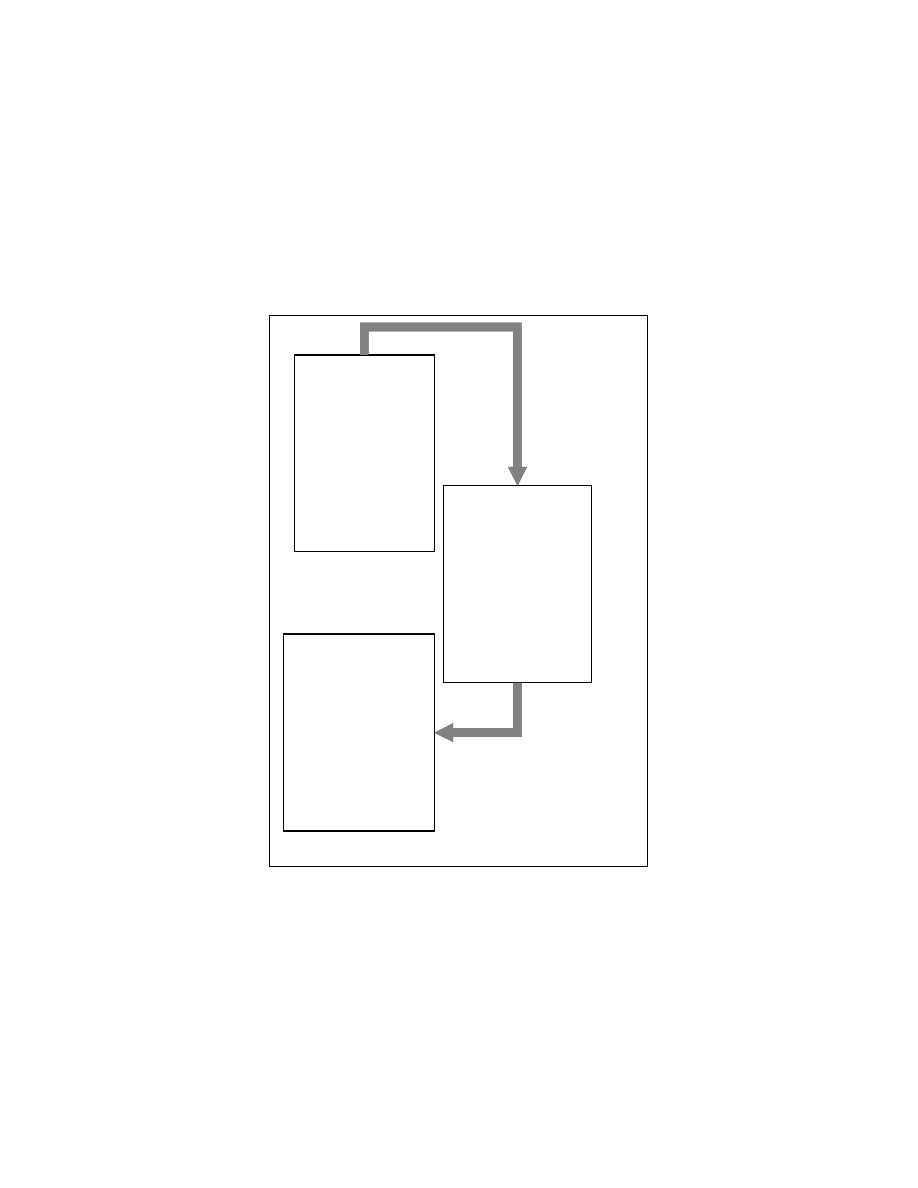
Figure 2-1 gives a diagrammatic representation of the working of a metamorphic
virus. The varying shapes in Figure 2-1 suggest different variants of the same virus. The
transformations that the virus applies to change its program code (shape) without
changing its behavior are called morphing transformations.
Definition Variant of a virus: A variant of a virus V is a virus V’ where V, V’ have the
same behavior but some difference in the code.
Definition Morphing Transformations: Morphing transformations are the
transformations that, when applied to a virus, yields a variant of that virus. These
transformations change the shape of a virus, but do not change its behavior.
Virus
Variant -3
Virus
Variant -1
Virus
Variant -2
M
M
S1
S2
S3
Legend
M – Morphing transformations
{S1, S2, S3} – Virus Signatures
Virus
Variant -3
Virus
Variant -1
Virus
Variant -2
M
M
S1
S2
S3
Legend
M – Morphing transformations
{S1, S2, S3} – Virus Signatures
Figure 2-1: Metamorphic viruses

6
Definition Morpher: The part of virus program logic responsible for generating different
variants of the virus using morphing transformations, is referred to as morpher.
Definition Metamorphic virus: A metamorphic virus is a virus that carries a morpher
with itself to generate a variant for each infection.
2.1 Morphing
transformations
Common morphing transformations used by virus writers are: dead code
insertion, variable renaming, statement reordering, expressions reshaping and break &
join transformations. This section discusses these transformations.
2.1.1 Dead code insertion
Dead code is the part of a program that is either not executed in the program or
has no effect on results of the program. Addition/Removal of such code to/from a
program doesn’t change its behavior.
Figure 2-2 shows an example of dead code insertion. Adding nops, and add eax, 0
to V1 creates V2, a morphed variant of V1. Similarly, addition of nops, add exa, 0 and
sub ebx, 0 to V2 creates V3. All the three variants, V1, V2 and V3, have same behavior.
If AV software uses the sequence of bytes corresponding to the instructions xor edx, edx
and div ecx as the virus signature, the morphed variants V2, and V3 will go undetected as
add eax, 0 is inserted after xor edx, edx.
7
….
mov eax, V_S - 1
nop
add eax, ecx
sub ebx, 0
xor edx, edx
add eax, 0
nop
div ecx
nop
mul ecx
push eax
….
….
mov eax, V_S - 1
add eax, ecx
xor edx, edx
div ecx
mul ecx
push eax
….
….
mov eax, V_S - 1
nop
add eax, ecx
xor edx, edx
add eax, 0
div ecx
nop
mul ecx
push eax
….
D
Legend
D : dead code inserion
{V1, V2, V3} : virus variants
V1
V2
V3
D
….
mov eax, V_S - 1
nop
add eax, ecx
sub ebx, 0
xor edx, edx
add eax, 0
nop
div ecx
nop
mul ecx
push eax
….
….
mov eax, V_S - 1
add eax, ecx
xor edx, edx
div ecx
mul ecx
push eax
….
….
mov eax, V_S - 1
nop
add eax, ecx
xor edx, edx
add eax, 0
div ecx
nop
mul ecx
push eax
….
D
Legend
D : dead code inserion
{V1, V2, V3} : virus variants
V1
V2
V3
D
Figure 2-2: Dead code insertion
8
2.1.2 Variable
renaming
Variable renaming transformation changes the names of a variable by changing
all the instances of the variable with a new name. Variants created by variable renaming
have the same behavior, as this transformation doesn’t change the program behavior.
Figure 2-3 shows two examples of variable renaming transformations. The
example code segment shown in Figure 2-3 is in IA-32 assembly language. Renaming
variables corresponds to renaming registers in assembly language. Instructions in variants
V1, V2 and V3 differ in their usage of registers. The register edx is renamed to eax from
….
push ecx
mov ecx, esi
mov edi, 000Ah
add ecx, edi
pop edi
….
….
push edx
mov edx, ecx
mov ebx, 000Ah
add edx, ebx
pop ebx
….
….
push eax
mov eax, ebx
mov edx, 000Ah
add eax, edx
pop edx
….
R
R
Legend
R : variable renaming transformations
{V1, V2, V3} : virus variants
V1
V2
V3
….
push ecx
mov ecx, esi
mov edi, 000Ah
add ecx, edi
pop edi
….
….
push edx
mov edx, ecx
mov ebx, 000Ah
add edx, ebx
pop ebx
….
….
push eax
mov eax, ebx
mov edx, 000Ah
add eax, edx
pop edx
….
R
R
Legend
R : variable renaming transformations
{V1, V2, V3} : virus variants
V1
V2
V3
Figure 2-3: Variable renaming
9
V1 to its morphed variant V2. If the signature for V1 has edx in its byte sequence, its
morphed variants V2 and V3 will not be detected using that signature.
2.1.3 Break & join transformations
Break & join transformations break a program into pieces, select a random order
of these pieces, and use unconditional branch statements to connect these pieces such that
the statements are executed in the same sequence as in the original program.
Figure 2-4 shows an example of break & join transformation. The order of
statements in variant V2 is different from the order in which these statements appear in
variant V1. Unconditional branch statements (GOTO statements) are used to connect
these pieces so that the statements in variants V1 and V2 are executed in the same order.
B
statement-1
statement-2
statement-3
statement-4
statement-5
statement-6
goto L1
L3:
statement-3
goto L4
L1:
statement-1
statement-2
goto L3
L5:
statement-5
goto L6
L4:
statement-4
goto L5
L6:
statement-6
Legend
B : break & join transformations
{V1, V2} : virus variants
V2
V1
B
statement-1
statement-2
statement-3
statement-4
statement-5
statement-6
goto L1
L3:
statement-3
goto L4
L1:
statement-1
statement-2
goto L3
L5:
statement-5
goto L6
L4:
statement-4
goto L5
L6:
statement-6
Legend
B : break & join transformations
{V1, V2} : virus variants
V2
V1
Figure 2-4: Break & join transformations
10
2.1.4 Expression
reshaping
Generating random permutations of operands in expressions with commutative
and associative operators reshapes expressions in programs. This changes the structure of
expressions. Expression reshaping doesn’t change the behavior of the program.
Figure 2-5 shows an example of expression reshaping transformations. The
expression x*100+2 in variant V1 is reshaped to 2+x*100 in variant V2. Behavior of the
….
if (i < b * a * c)
{
a = 100 * x + 2;
b = i * 10;
c = b+ y * a;
i = a + c + b;
}
….
….
if (i < a * b * c)
{
a = x * 100 + 2;
b = 10 * i;
c = y * a + b;
i = a + b + c;
}
….
….
if (i < a * b * c)
{
a = 2 + x * 100;
b = 10 * i;
c = a * y + b;
i = b + c + a;
}
….
S
S
Legend
S : expression reshaping
{V1, V2, V3} : virus variants
V2
V3
V1
….
if (i < b * a * c)
{
a = 100 * x + 2;
b = i * 10;
c = b+ y * a;
i = a + c + b;
}
….
….
if (i < a * b * c)
{
a = x * 100 + 2;
b = 10 * i;
c = y * a + b;
i = a + b + c;
}
….
….
if (i < a * b * c)
{
a = 2 + x * 100;
b = 10 * i;
c = a * y + b;
i = b + c + a;
}
….
S
S
Legend
S : expression reshaping
{V1, V2, V3} : virus variants
V2
V3
V1
Figure 2-5: Expression reshaping

11
variants V1, V2, and V3 remains the same. If the virus signature of variant V1 includes
the expression x*100+2, variants V2 and V3 will not be detected by AV software.
2.1.5 Statement reordering
Statement reordering transformation reorders statements in a program such that
the behavior of the program doesn’t change. It is possible to reorder statements if and
only if there are no dependences [9] between the statements being reordered. If the virus
signature includes bytes corresponding to a statement from this set of reorderable
statements, application of statement reordering transformation makes the original virus
signature useless for morphed variants.
Figure 2-6 shows an example of statement reordering transformations. The
statements a=y*i, b=200*i, and a=x*y+i*z can be reordered as there are no
dependencies between these statements. Selection of random permutations of such
reorderable statements creates the morphed variants V2 and V3.
12
….
z= 100;
x = 25;
y = x +get_index();
while (i < y + z)
{
b = 200 * i;
a = x * y + i * z;
c = y * i;
i = i + 1;
}
….
….
x = 25;
y = x + get_index();
z= 100;
while (i < y + z)
{
a = x * y + i * z;
b = 200 * i;
c = y * i;
i = i + 1;
}
….
….
x = 25;
z= 100;
y = x + get_index();
while (i < y + z)
{
c = y * i;
b = 200 * i;
a = x * y + i * z;
i = i + 1;
}
….
O
O
Legend
O : statement reordering
{V1, V2, V3} : virus variants
V2
V3
V1
….
z= 100;
x = 25;
y = x +get_index();
while (i < y + z)
{
b = 200 * i;
a = x * y + i * z;
c = y * i;
i = i + 1;
}
….
….
x = 25;
y = x + get_index();
z= 100;
while (i < y + z)
{
a = x * y + i * z;
b = 200 * i;
c = y * i;
i = i + 1;
}
….
….
x = 25;
z= 100;
y = x + get_index();
while (i < y + z)
{
c = y * i;
b = 200 * i;
a = x * y + i * z;
i = i + 1;
}
….
O
O
Legend
O : statement reordering
{V1, V2, V3} : virus variants
V2
V3
V1
Figure 2-6: Statement reordering

3 Background
This chapter gives the definitions of the terms used and briefly discusses these
concepts.
3.1
Control flow graph (CFG)
A control flow graph [2] is a directed graph containing a set of vertices V and a
set of edges, E. Each vertex (also classed a node) in the control flow graph represents a
sequence of instructions that are executed sequentially (also called basic block). Control
flow graph edges represent the control flow in the program. A control flow graph has two
special nodes called start and end. There is a path from start node to every node in V and
a path from every node to the end node. Figure 3-2 shows the control flow graph for the
program segment shown in Figure 3-1.
3.2 Dominator
A node n1 in the control flow graph is said to dominate the node n2 iff all the
paths in the control flow graph from the start node to node n2 include node n1 [8].
Figure 3-3 shows the dominator relationships for the blocks of the control flow graph
shown in Figure 3-2. In the tree shown in Figure 3-3, the ancestors of a node dominate
that node and the parent node of a node immediately dominates that node.
14
m in = A [0];
for ( i = 0; i < n; i+ + )
{
if (m in > A [i])
{
m in = A [i];
}
}
Figure 3-1: Sample program segment
Start
min = A [0]
i = 0
if (i<n) : B1 : B2
if (min>A[i]) : B3 : B4
min = A[i]
i = i + 1
if (i<n) : B1 : B2
End
B
start
B
end
B0
B1
B3
B4
B2
Start
min = A [0]
i = 0
if (i<n) : B1 : B2
if (min>A[i]) : B3 : B4
min = A[i]
i = i + 1
if (i<n) : B1 : B2
End
B
start
B
end
B0
B1
B3
B4
B2
Figure 3-2: Control flow graph for the program segment in Figure 3-1
15
3.3 Post-Dominator
A node n1 in the control flow graph is said to post-dominate the node n2 if and
only if all the paths in the control flow graph from node n2 to the end node include node
n1 [8].
Figure 3-4 shows the post-dominator relationships for the blocks of the control
flow graph shown in Figure 3-2. In the tree shown in Figure 3-4, the ancestors of a node
post-dominate that node, and the parent node of a node immediately post-dominates that
node.
B
start
B0
B1
B2
B3
B4
B
end
B
start
B0
B1
B2
B3
B4
B
end
B
start
B0
B1
B2
B3
B4
B
end
Figure 3-3: Dominator tree for Figure 3-2
B
start
B0
B1
B2
B3
B4
B
end
B
start
B0
B1
B2
B3
B4
B
end
B
start
B0
B1
B2
B3
B4
B
end
Figure 3-4: Post-Dominator tree for Figure 3-2

16
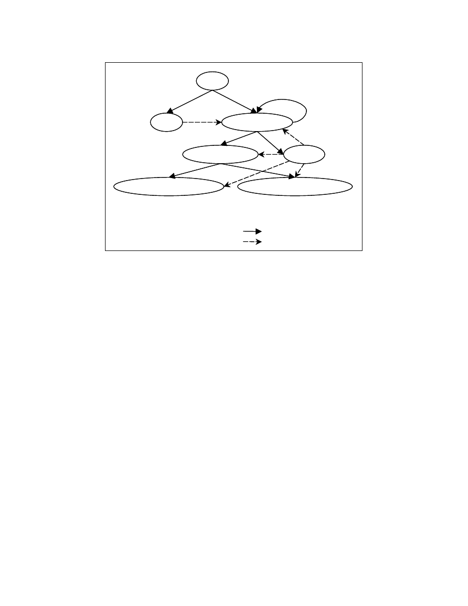
3.4
Program dependence graph
Program dependence graph [4] is a directed graph containing a set of vertices and
a set of edges. The vertices in a program dependence graph represent the program points
and the edges represent the dependencies between the program points. The edges can be
of two types – control dependence edges and data dependence edges. Figure 3-6 shows
the program dependence graph for the program in Figure 3-5.
A program point p1 is said to be data dependent on the program point p2 if and
only if there exists a path from program point p2 to program point p1 in the control flow
graph and there exists at least one variable defined at the program point p2 that is used at
the program point p1 and the variable is not killed along that path.
The program point p2 is said to be control dependent on the program point p1 if
and only if there exists a path in the control flow graph from p1 to p2 and p2 post-
dominates all nodes on that path except p1.
void main() {
int i = 1;
while (i<100) {
if(i%2 == 0)
printf(“%d is even\n”, i);
else
printf(“%d is odd\n”, i);
i = i + 1;
}
}
Figure 3-5: A sample program
17
3.5
Data dependence predecessors
Data dependence predecessors of a program point ‘p’ are program points that
have a data dependence edge to p.
3.6
Data dependence successors
Data dependence successors of a program point ‘p’ are program points that have a
data dependence edge from p.
Start
i = 1
while (i<100)
if(i%2 ==0)-else
printf(“%d is even\n”, i);
printf(“%d is odd\n”, i);
i = i + 1
Legend
Control Dependence
Data Dependece
Start
i = 1
while (i<100)
if(i%2 ==0)-else
printf(“%d is even\n”, i);
printf(“%d is odd\n”, i);
i = i + 1
Legend
Control Dependence
Data Dependece
Figure 3-6: Program dependence graph for the program in Figure 3-5
4 Zeroing
transformations
We now propose zeroing transformations, a set of transformations to nullify the
effect of morphing transformations. Zeroing transformations, when applied to a virus,
result in its zero form. Application of these transformations on the set of morphed
variants of a virus related by morphing transformations result in the same zero form.
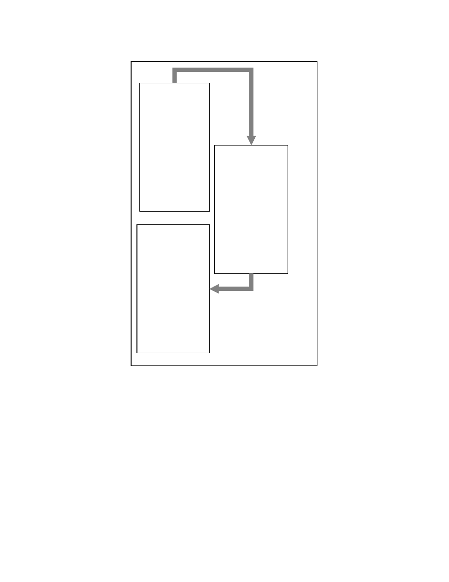
Figure 4-1 illustrates the idea of applying zeroing transformations to create zero forms of
the viruses. V1, V2, and V3 in Figure 4-1 are transformed to V
⊕
. AV companies can use
this method and store the virus signature extracted from V
⊕
instead of maintaining
separate virus signatures for V1, V2 and V3. To use these zero signatures for virus
detection, the AV software will need to apply zeroing transformations on the programs to
be checked for the existence of virus behavior to get their zero forms. Zero forms of the
programs can then be searched for zero signatures of the viruses.
Virus
Variant -3
Virus
Variant -1
Virus
Variant -2
M
M
S1
S2
S3
Legend
M – Morphing transformations
⊕
– Zeroing Transformations
{S1, S2, S3} – Virus Signatures
S
⊕
– Zero signature
Zero form
S
⊕
⊕
⊕
⊕
Virus
Variant -3
Virus
Variant -1
Virus
Variant -2
M
M
S1
S2
S3
Legend
M – Morphing transformations
⊕
– Zeroing Transformations
{S1, S2, S3} – Virus Signatures
S
⊕
– Zero signature
Zero form
S
⊕
⊕
⊕
⊕
Figure 4-1: Detection approach
19
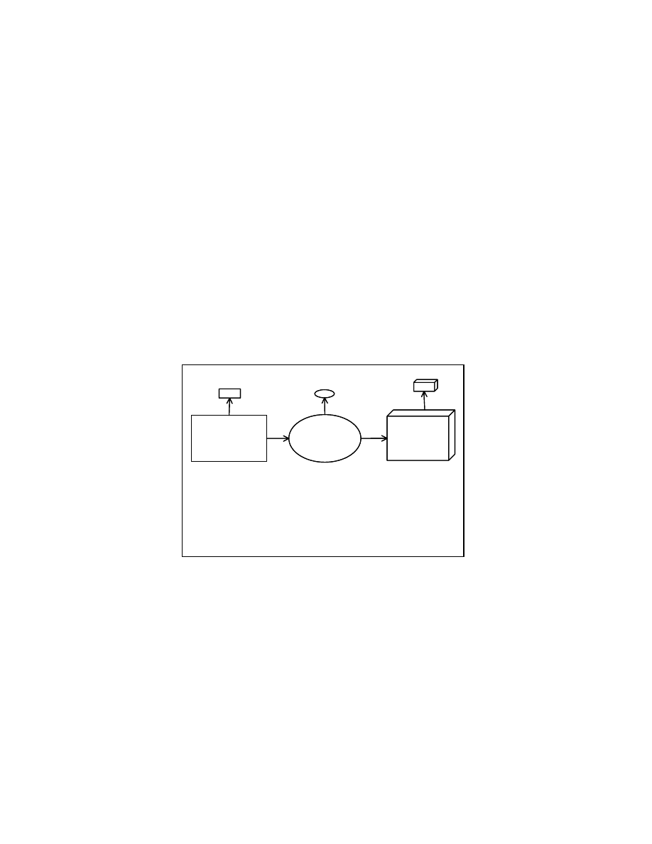
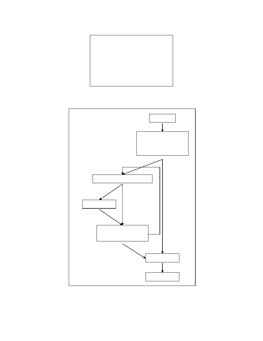
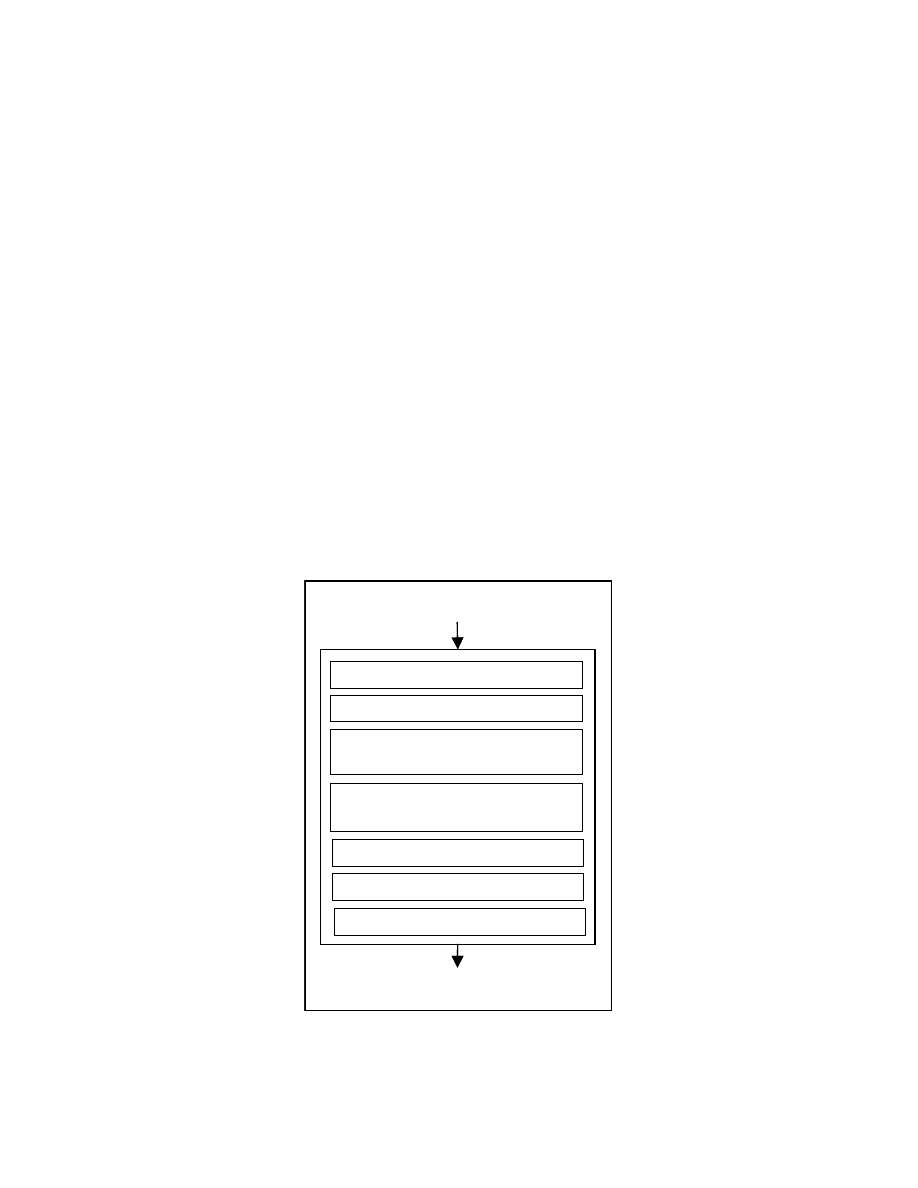
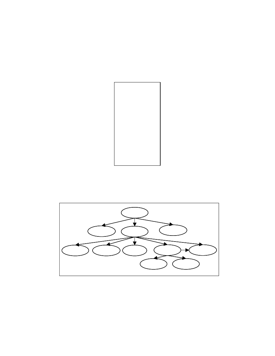
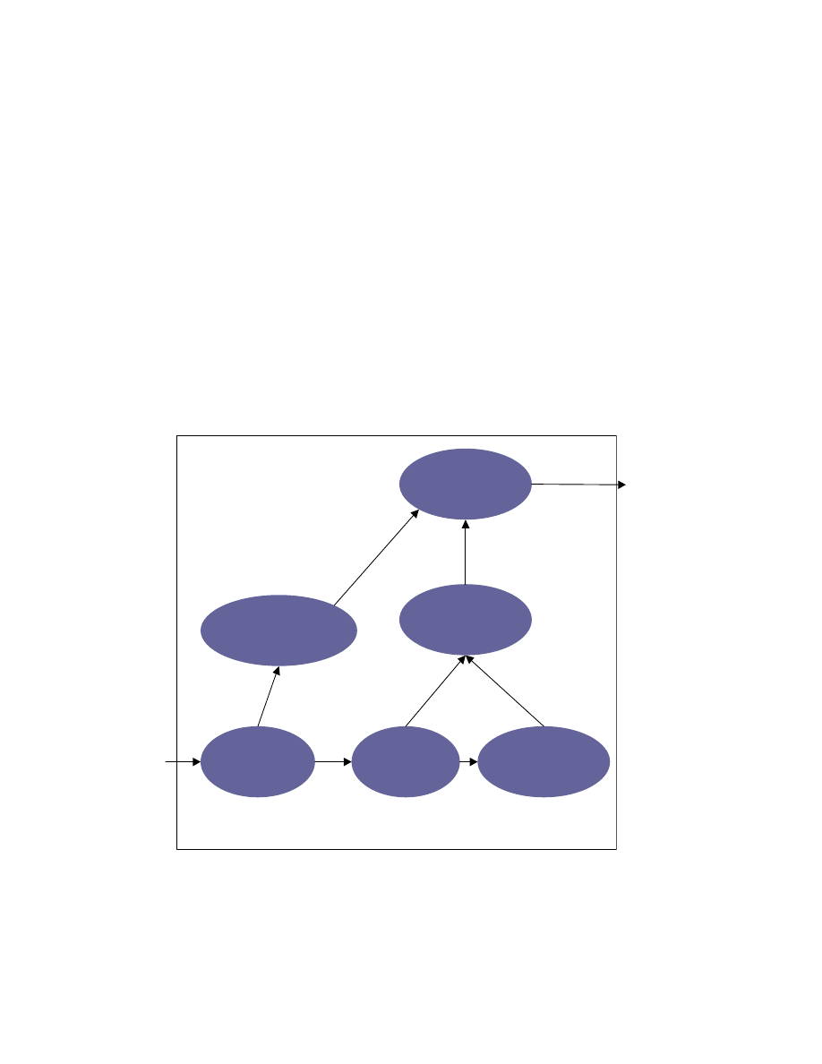
Figure 4-2 shows the procedure for creating the zero form of a program. A series
of transformations are applied to the input program. These transformations include dead-
code elimination [8], constant propagation and removal of redundant computations [8],
elimination of spurious unconditional branch statements, reshaping expressions to zero
form, fixing an order for the statements that can be reordered and renaming variables to a
zero form. This thesis contributes a method for fixing an order for the statements in the
program.
For fixing the statement order, we need to find the reorderable statements in the
program and impose an ordering on them. To find the reorderable statements, we use a
tree representation called program tree. We also create a graph showing the dependence
relation between the nodes in the program tree.
Propagate constants
Eliminate dead code
Remove redundant
computations
Remove spurious unconditional
branch statements
Reshape Expressions
Fix statement order
Rename Variables
Program
Zero Form
Propagate constants
Eliminate dead code
Remove redundant
computations
Remove spurious unconditional
branch statements
Reshape Expressions
Fix statement order
Rename Variables
Program
Zero Form
Figure 4-2: Zeroing transformations

20
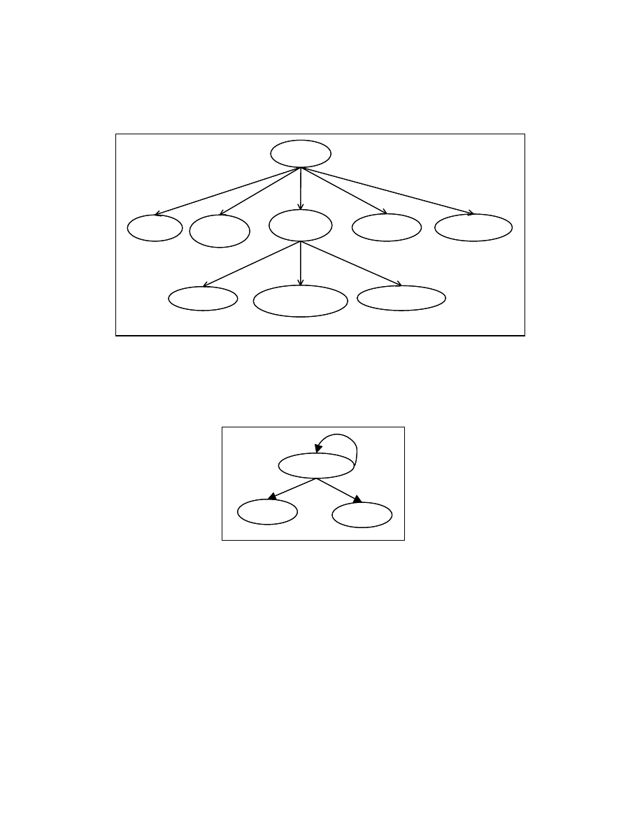
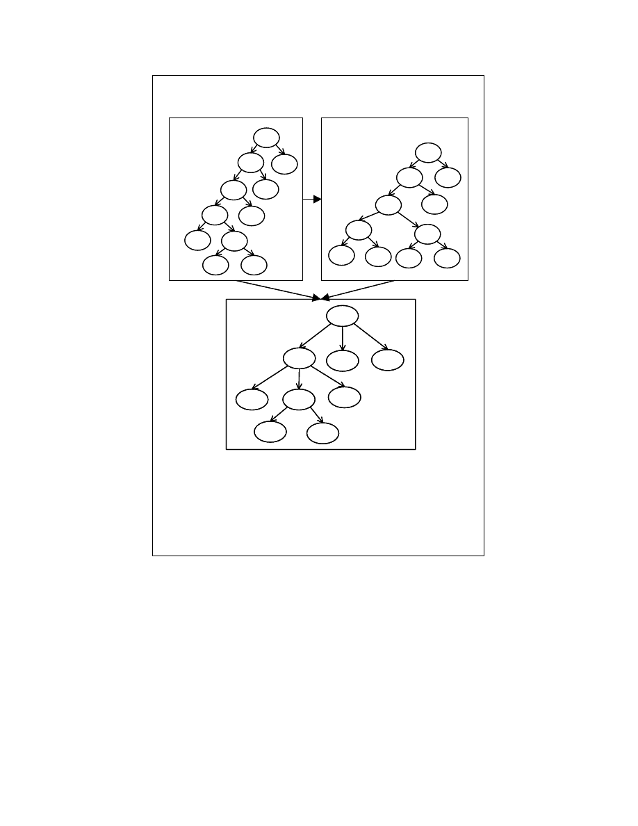
4.1
Program Tree (PT) representation
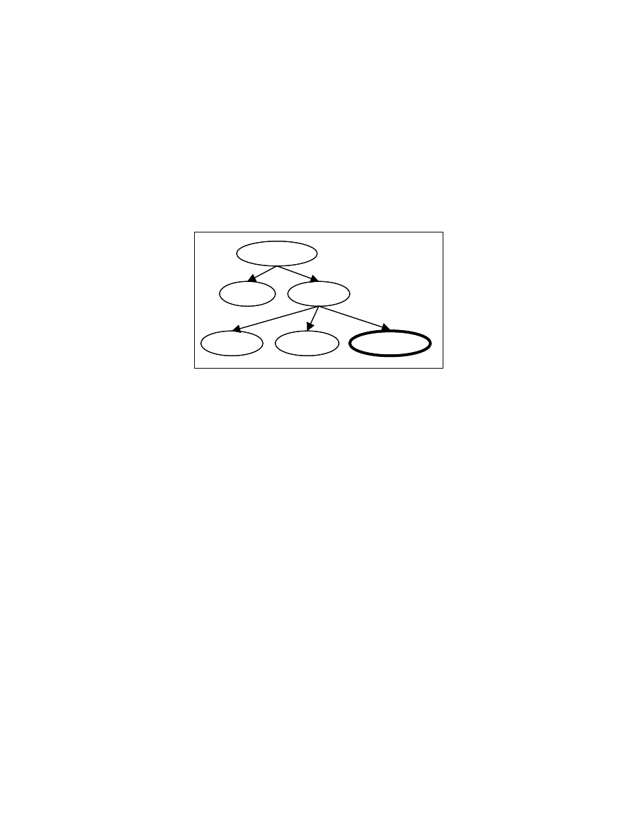
For each procedure/function in a program we create a program tree (PT). The PT
representation of the function in Figure 4-3 is shown in Figure 4-4. We use the control
dependence sub-graph (CDG) for constructing the PT. Construction of PT for structured
programs is straightforward. The nodes in the program tree are the statements of the
program. We create an edge in the program tree from a node n
1
to node n
2
if there exists
an edge from n
1
to n
2
in the corresponding control dependence subgraph. In order to
make the program tree more readable, we show the corresponding program statements for
control predicates in the program tree. For example, in Figure 4-4, the control predicate
(A>B) is shown as If (A>B).
The node If (A>B) in Figure 4-4 has an edge to the nodes C=A+1, D=A+B+200,
E=C+D+10 because of the control dependence relationship between the node If (A>B)
and the nodes C=A+1, D=A+B+200, E=C+D+10. Some nodes have self-loops in their
control dependence sub-graph. An example of a self-loop in the control dependence
subgraph is shown in the Figure 4-5. We do not place any edges in the program tree for
the control dependence edges involving self-loops in the control dependence subgraph.
A=0
B=3
IF (A>B) then
C = A + 1
D = A + B + 200
E = C + D + 10
FI
F = A + C
G = A + B
Figure 4-3: A sample program segment
21
We construct a program tree for each procedure of the program. For handling
unstructured programs we use a different approach.
4.1.1 Handling unstructured programs
While constructing the program tree from the control dependence subgraph, we
may encounter cycles in the control dependence subgraph involving more than one node.
Moreover, a node can be control dependent on multiple nodes. These cases arise for some
unstructured programs. For example, consider the program segment in Figure 4-6. The
main()
A=0
B=3
If (A>B)
F=A+C
G=A+B
C=A+1
D=A+B+200
E=C+D+10
main()
A=0
B=3
If (A>B)
F=A+C
G=A+B
C=A+1
D=A+B+200
E=C+D+10
Figure 4-4: Program tree for the program segment in Figure 4-3
while (x<10)
x=x+1
print(x)
while (x<10)
x=x+1
print(x)
Figure 4-5: A self-loop in the control dependence subgraph
22
control dependence subgraph for this program segment, shown in Figure 4-7, has a node
that is control dependent on multiple nodes. Figure 4-9 gives an example of a cycle in the
control dependence subgraph. Any node in a tree cannot have multiple parents and it
cannot be involved in a cycle.
main()
{
read (x)
if (x>5)
goto L1
read (x)
x = x – 1
if (x>10)
goto L1
goto L2
L1:
read(x)
L2:
write(x)
}
Figure 4-6: A sample unstructured program segment.
x = x – 1
if (x>5)
goto L1
read(x)
if (x>10)
goto L1
goto L2
L1:read(x)
L2:write(x)
read (x)
main()
x = x – 1
if (x>5)
goto L1
read(x)
if (x>10)
goto L1
goto L2
L1:read(x)
L2:write(x)
read (x)
main()
x = x – 1
if (x>5)
goto L1
read(x)
if (x>10)
goto L1
goto L2
L1:read(x)
L2:write(x)
read (x)
main()
Figure 4-7: Control dependence subgraph for the program segment in Figure 4-6
23
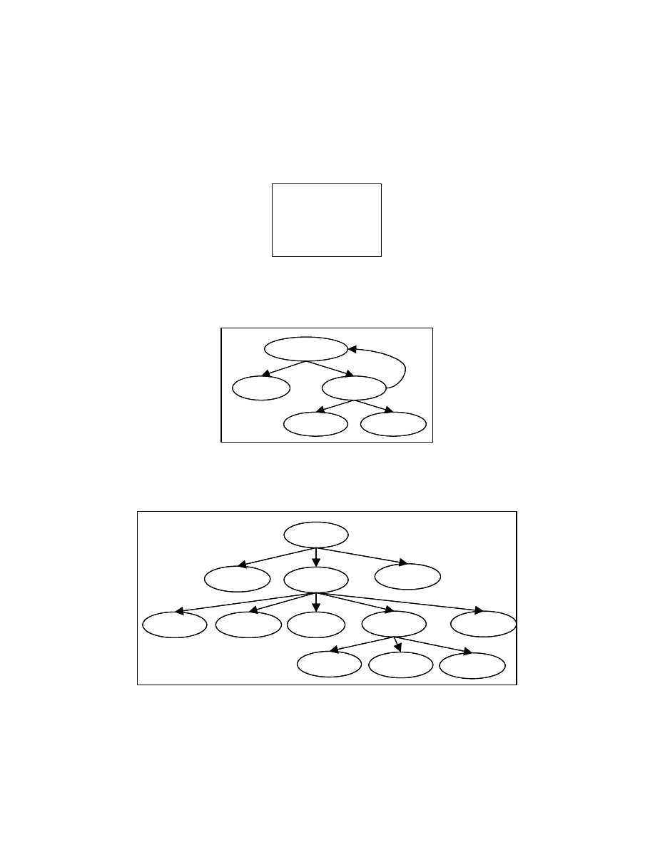
If a node in the control dependence subgraph has multiple parents, we create a
duplicate child node for each parent node. Figure 4-10 shows the PT for the program
segment shown in Figure 4-6 obtained by following this strategy.
while (x<10)
x = x+1
if (x>5)
break
print (x)
Figure 4-8: A sample program segment
while (x<10)
x=x+1
print(x)
if (x>5)
break
while (x<10)
x=x+1
print(x)
if (x>5)
break
Figure 4-9: Control dependence graph for program segment in Figure 4-8
x = x – 1
if (x>5)
goto L1
read(x)
if (x>10)
goto L1
goto L2
L1:read(x)
L2:write(x)
read (x)
main()
L1:read(x)
x = x – 1
if (x>5)
goto L1
read(x)
if (x>10)
goto L1
goto L2
L1:read(x)
L2:write(x)
read (x)
main()
L1:read(x)
Figure 4-10: PT for program segment in Figure 4-6
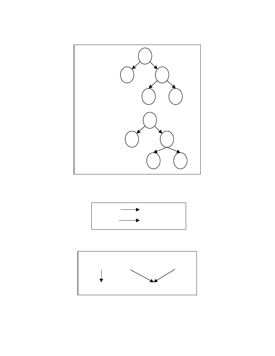
24
To handle loops in a control dependence subgraph, we use the following method.
If a node p1 has p2 as its successor in the control dependence subgraph, such that p2 is an
ancestor of p1 in the program tree constructed so far, we create a special node for p2 and
add it as children of p1. We do not explore this special node any further. Figure 4-11
shows the program tree obtained for Figure 4-8 using this strategy.
4.2
Algorithm for imposing an order on the statements
The algorithm for imposing an ordering on the nodes in a PT is shown in the
Figure 4-12. This algorithm has two steps.
1)
Partition PT nodes into reorderable sets.
2)
Use ordering strategies to get an ordering of statements in each
reorderable set.
This algorithm uses string representations of the statements (explained in Section 4.4) for
imposing an ordering on the program statements.
while (x<10)
x=x+1
print(x)
if (x>5)
break
while (x<10)
while (x<10)
x=x+1
print(x)
if (x>5)
break
while (x<10)
Figure 4-11: PT for the program segment in Figure 4-8

25
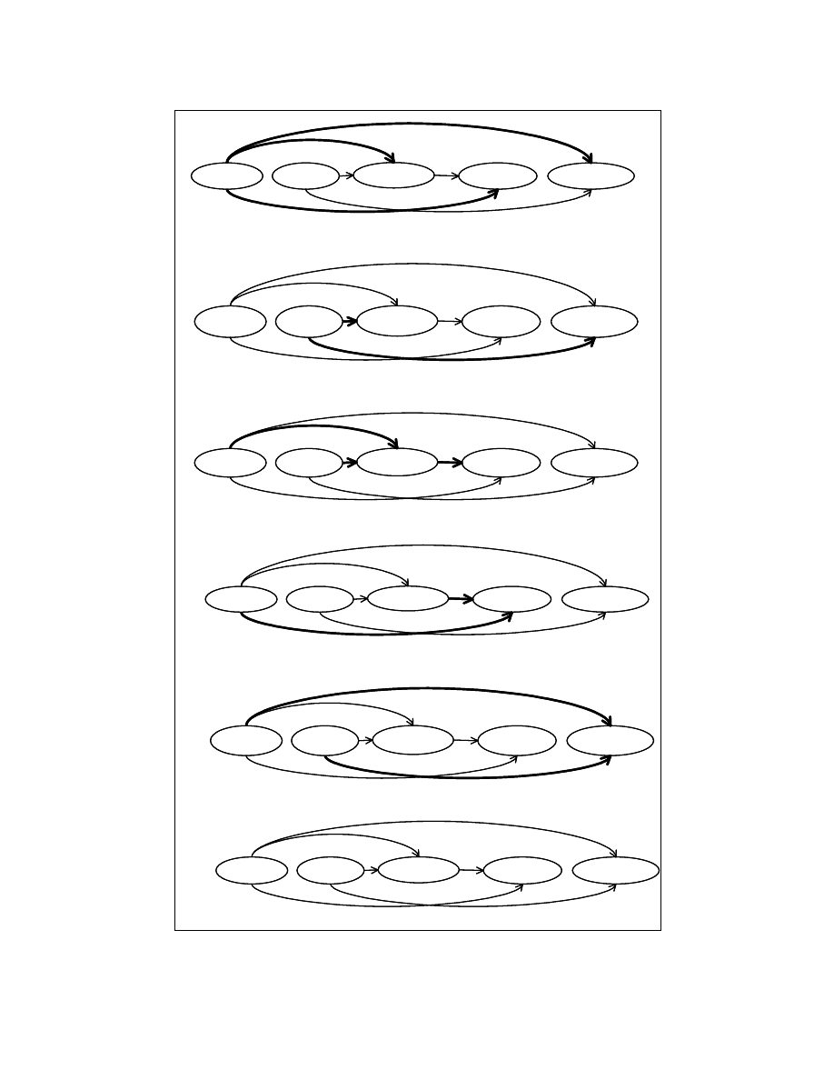
4.3
Partitioning PT into reorderable sets
This section describes a partitioning algorithm for creating reorderable sets of PT
nodes. The aim of this step is to find statements in the program that can be reordered
without changing the program semantics.
Sibling PT nodes can be reordered if there are no dependencies between these
nodes. Dependence relation between two nodes n1, n2
∈ PT, with the same parent node
is defined as follows. Node n2 is said to be dependent on node n1 if and only if there
exists a path from n1 to n2 in the control flow graph of P and either a node in the sub-tree
of PT rooted at n2 is data dependent on a node in the sub-tree of PT rooted at n1 or there
Algorithm Impose-Order (P)
PT = Program Tree of P
Build the string representations for each node in the PT.
Partition the PT into reorderable sets.
Create-String-Form (PT-root)
Sort the elements in each reorderable set by comparing the SR1 of the nodes in PT.
For the sets of statements that cannot be sorted using SR1
Sort the reorderable set by comparing the SR2 of the nodes in PT.
For the sets of statements that cannot be sorted using SR2
Sort the reorderable set by comparing the SR3 of the nodes in PT.
For the sets of statements that cannot be sorted using SR3
Sort the reorderable set by comparing the SR4 of the nodes in PT.
End Algorithm Impose-Order
Figure 4-12: Algorithm for fixing the order of statements in a program

26
exist two nodes n1’ and n2’ in the sub-trees of PT rooted at n1 and n2 respectively such
that the intersecting set of variables defined in n1’ and n2’ in non-empty.
The sets of nodes that can be reordered are computed. Each of such set is a
reorderable set. The process of creating these reorderable sets is called partitioning.
Definition Reorderable set: A set of nodes in PT are said to form a reorderable set if and
only if they have the same parent node and they can be reordered without changing the
semantics of the program represented by PT.
The children of the nodes in the PT are partitioned into one or more reorderable
sets. The order of the reorderable set is fixed, but the order of the elements within the
reorderable set is not fixed. Given a program (P) and its corresponding PT, the PT nodes
can be partitioned into reorderable sets using the partitioning algorithm. The partitioning
algorithm traverses the PT of P in the post order to find the nodes that can be reordered.
The partitioning algorithm places each node in its corresponding reorderable set. It
maintains data dependence information using a dependence graph. The dependence graph
has an edge from node n1 to node n2 if n2 depends on n1. Figure 4-13 shows the
dependence graph for the node main () in the Figure 4-4. We use dependence graph depth
(DG-Depth) of a node, which is initially set to ‘0’ for all the nodes, for placing the nodes
into reorderable sets. The children of a node are processed in the control flow order. For
every child node C of N, the partitioning algorithm finds the node C’, having the
maximum DG-Depth ‘m’, such that either C depends on C’ or C’ depends on C. The
child node C is placed in the reorderable set numbered m+1 and the DG-Depth of C is set
to m+1. This assures that after the nodes are partitioned, the dependence order of the
reorderable sets is preserved.
27
Consider the Node main () in Figure 4-4. It has {A=0, B=3, If (A>B), F=A+C,
G=A+B} as its children. The dependence graph for this set of children is shown in Figure
4-13. The edge from the node A=0 to the node If (A>B) corresponds to the dependence
relation from node A=0 to the node If (A>B); i.e., there exists a path from the node A=0
to the node If (A>B) in the control flow graph of P and a value defined by the node A=0
is used by at least one node in the sub-tree starting with the node If (A>B). Similarly, the
edge from the node If (A>B) to the node F = A+C corresponds to a dependence relation
from If (A>B) to F=A+C.
A=0
B=3
If (A>B)
F=A+C
G=A+B
A=0
B=3
If (A>B)
F=A+C
G=A+B
Figure 4-13: Data dependence graph for the children of “root” in Figure 4-4
28
(a) Processing the node [A=0]
(b) Processing the node [B=3]
Set the DG-Depth of [B=3] to 1 (max (0, 0) + 1)
0
0
0
0
0
A=0
B=3
If (A>B)
F=A+C
G=A+B
Set the DG-Depth of [A=0] to 1 (max (0, 0, 0) + 1)
1
0
0
0
0
A=0
B=3
If (A>B)
F=A+C
G=A+B
(c) Processing the node [If (A>B)]
Set the DG-Depth of [If (A>B)] to 2 (max (1, 1, 0) + 1)
1
1
0
0
0
A=0
B=3
If (A>B)
F=A+C
G=A+B
(d) Processing the node [F=A+C]
Set the DG-Depth of [F=A+C] to 3 (max (2, 1) + 1)
1
1
2
0
0
A=0
B=3
If (A>B)
F=A+C
G=A+B
(e) Processing the node [G=A+B]
Set the DG-Depth of [G=A+B] to 2 (max (1, 1) + 1)
1
1
2
3
0
A=0
B=3
If (A>B)
F=A+C
G=A+B
(f) Dependence graph depths after partitioning
1
1
2
3
2
A=0
B=3
If (A>B)
F=A+C
G=A+B
Depth :
Depth :
Depth :
Depth :
Depth :
Depth :
Figure 4-14: Working of partitioning algorithm

29
The working of the partitioning algorithm is shown in Figure 4-14. The child
nodes are processed in the control flow order. At each step, we pick a node and find the
reorderable set to which it belongs. Initially, all the child nodes are given a DG-Depth of
‘0’. Figure 4-14(a) shows the processing of the child node A=0. The incoming/outgoing
edges of the node A=0 are directed from/to the nodes having a DG-Depths as ‘0’. Hence,
the node A=0 is placed in the reorderable set numbered ‘1’. The DG-Depth of the node
A=0 is set to ‘1’. In Figure 4-14(d), the algorithm processes the child node F=A+C. The
DG-Depths of the nodes that have a dependence relation with F=A+C are {2, 1}. The
maximum value in this set is 2. Hence F=A+C is placed in the reorderable set numbered
3. The DG-Depth of the node F=A+C is set to ‘3’.
After partitioning, the reorderable sets will be as follows.
Reorderable set–1: {A=0, B=3};
Reorderable set–2: {If (A>B), G=A+B};
Reorderable set–3: {E=A+C}.
Figure 4-14(f) shows the partitioned dependence graph.
The partitioning algorithm described above gives the same reorderable sets
independent of statement reordering expression reshaping and variable renaming
transformations. The next step in getting the ZERO form for a program is to impose an
order on the nodes in the reorderable sets. Since we get the same reorderable sets even in
the presence of statement reordering, expression reshaping, and variable renaming, the
same order will be imposed for all the metamorphic variants of a virus. In the next
section, we describe the ordering strategies that we have used for creating the ZERO
form.

30
4.4 Ordering
strategies
The ordering strategies we have used for getting the ZERO form require a string
representation of the statements in the program. In this section, we describe the procedure
for constructing string from the program statements. The basic idea behind using string
representation for program statements is to impose an ordering on the statements in the
same reorderable sets by comparing their string representations. Since morphing
transformations can rename variables, we cannot use variable names in the string
representation of the statements. In order to get the string representation of a statement,
for each of the variables in the statement, we use the PT depths of the reaching
definitions [9] of that variable as a string to represent that variable. This is based on the
observation that the PT depths of the statements remain the same even if the metamorphic
transformation for statement reordering is applied.
Another problem that needs to be addressed when constructing the string
representation of statements is expression reshaping. We give a reshaping strategy for
constructing string representation for expressions with commutative operators. Figure
4-15 illustrates the method for getting a string form for an expression. The Abstract
Syntax Tree representation of the expression given in Figure 4-15(a) has to be
restructured so that the expression reshaping transformation doesn’t affect the string
representation of the expression. For achieving this, we construct a tree (which can have
more than two children) from AST of the expression. This tree representation constructed
from the AST in Figure 4-15(a) is shown in Figure 4-15(b). Using this restructured tree
for constructing the string form ensures that the expression reshaping done to the
commutative and associative operators is zeroed out.
31
Once we get the restructured ASTs, we create a string representation for the
expression represented by the AST. We use the algorithm shown in Figure 4-16 for
creating string representations of expressions. Figure 4-18 shows an example of string
representations for two expressions. This figure uses the string “I” to represent the
variables in the program.
x
y
z
z
e
d
+
*
*
-
+
x
y
z
z
-e
d
+
*
+
(c) Restructured AST for x * (y + z) * d – e + z
x
z
e
*
*
-
+
z
y
+
d
(a) AST for
x * (y + z) * d – e + z
(b) AST for
x * d * (z + y) – e + z
R
Legend
R : Reshape expressions
S : Restructure AST
S
S
x
y
z
z
e
d
+
*
*
-
+
x
y
z
z
-e
d
+
*
+
(c) Restructured AST for x * (y + z) * d – e + z
x
y
z
z
-e
d
+
*
+
(c) Restructured AST for x * (y + z) * d – e + z
x
z
e
*
*
-
+
z
y
+
d
(a) AST for
x * (y + z) * d – e + z
(b) AST for
x * d * (z + y) – e + z
R
Legend
R : Reshape expressions
S : Restructure AST
S
S
Figure 4-15: Restructuring AST to handle expression reshaping

32
After creating the string representations for the expressions in the statements, we
apply the algorithm shown in Figure 4-17 to get the string representations for the nodes in
program tree.
Algorithm Create-Expression-String-Form (expression)
If (expression is leaf)
If (expression represents a variable)
String-Representation of expression = “I”.
Else
String-Representation of expression = constant value in expression
End If
Else
S = String representation of the operator in expression
For each child C of PT-Node
Create-Expression-String-Form (C)
End For
If (PT-Node represents a commutative operator)
L = Sorted list of string representations of the children of PT-Node
Else
L = List of string representations of the children of PT-Node.
End If
S’ = String formed by appending strings in L.
String-Represetation of expression = String formed by appending S and S’
End If
End Create-Expression-String-Form
Figure 4-16: Algorithm for creating string representation of expressions

33
We name the string representation obtained by using this procedure as SR1. To
impose an order on the statements present in the same reorderable set, we compare the
SR1s of the statements in the reorderable sets. The statements in the same reorderable
sets may have the same SR1. For instance, the statements A=B+20 and C=20+D have
the same SR1s. In that case, we will not be able to impose an order on the statements
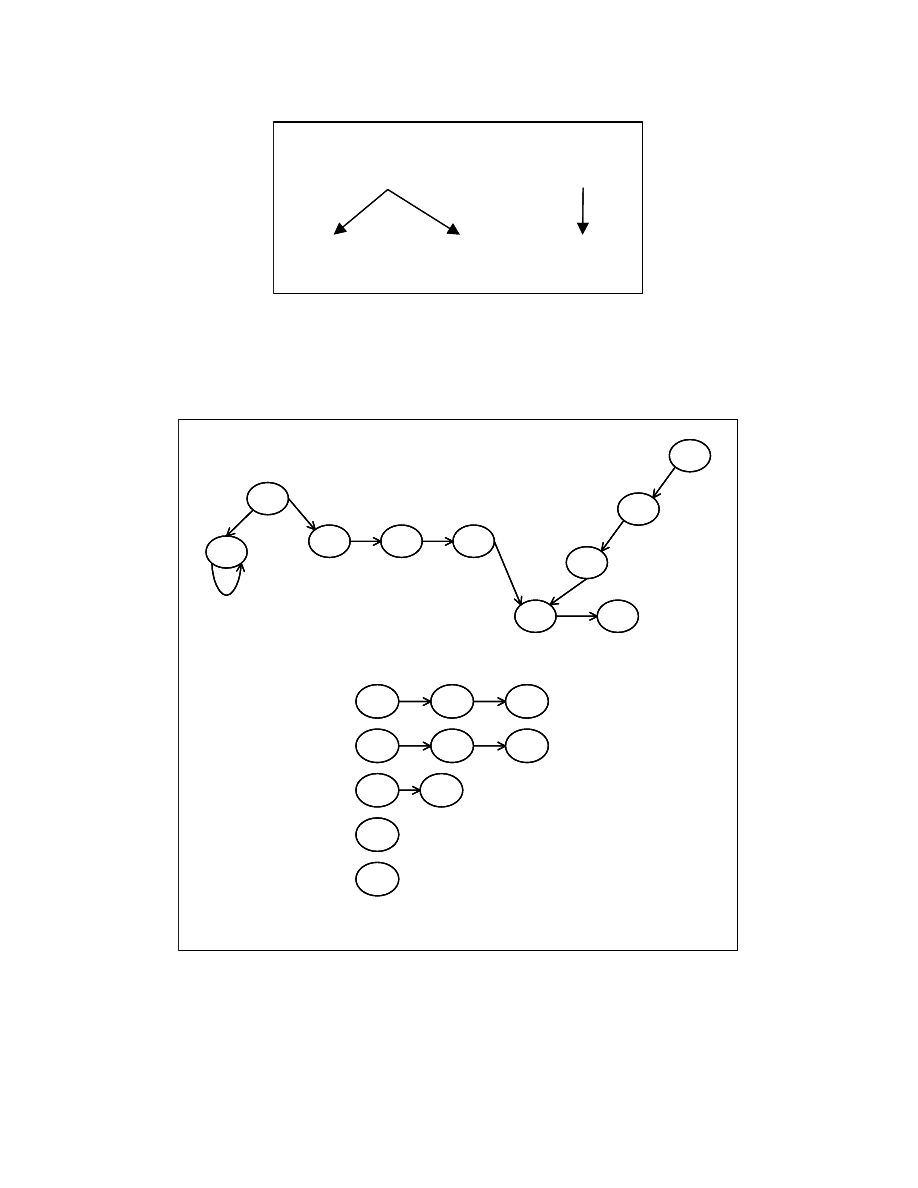
appearing in the reorderable sets using SR1. To minimize such cases, we modify the
partitioning algorithm. Instead of partitioning the statements, we partition the dependence
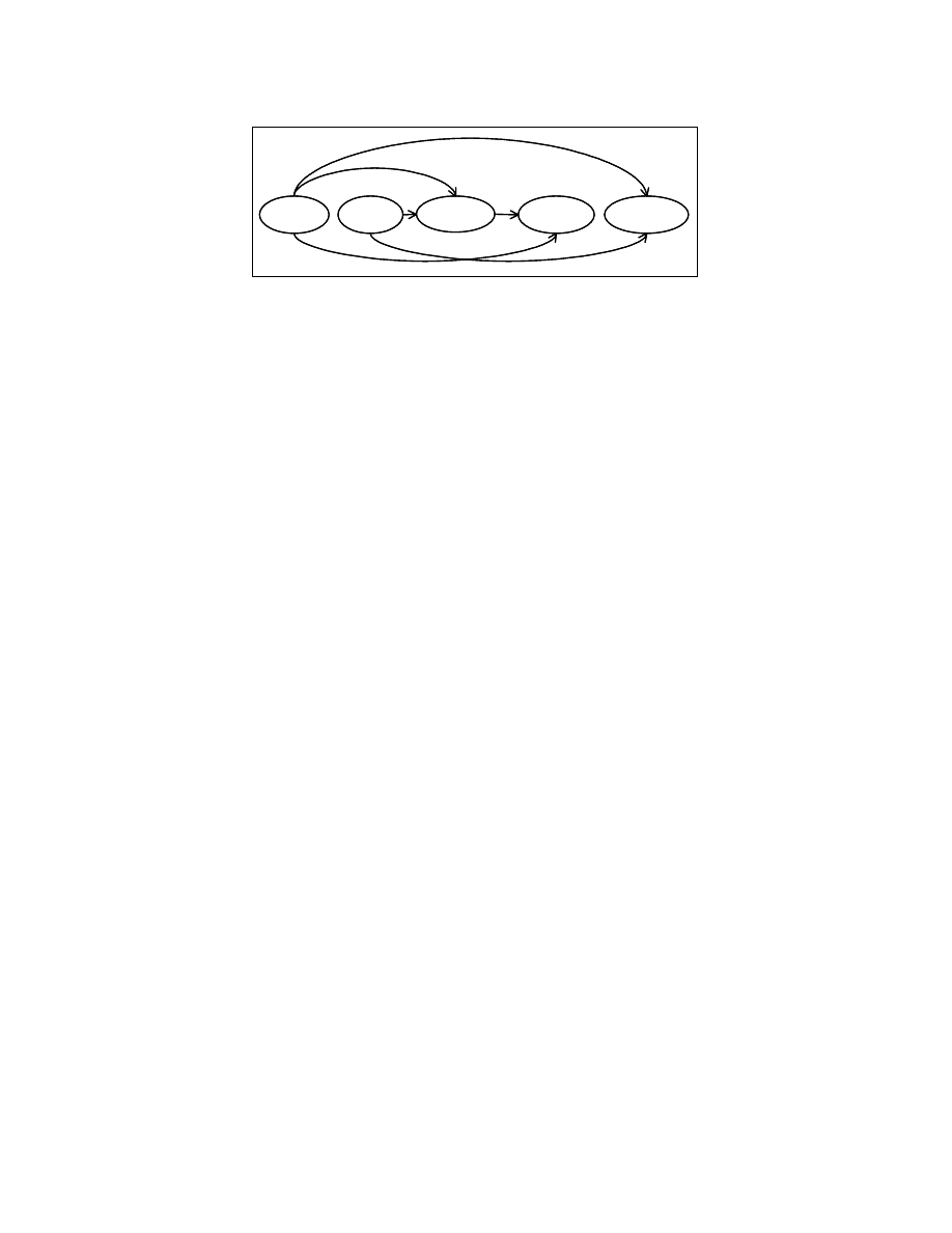
chains. A dependence chain is defined as follows. Two nodes n1 and n2 will be part of
the same dependence chain if and only if n1 has only one dependent n2, and n2 is
dependent on only one node n1. Figure 4-22 (b) shows the dependence chains formed for
Algorithm Create-String-Form (PT-Node)
If (PT-Node is leaf)
Create-Expression-String-Form(expression in PT-Node)
SR1 of PT-Node = String-Representation of expression in PT-Node.
Else
S = String representation of the expression in PT-Node
For each child C of PT-Node
Create-String-Form (C)
End For
L = Sorted list of SR1s of the children of PT-Node
S’ = String formed by appending strings in L.
SR1 of PT-Node = String formed by appending S and S’
End If
End Create-String-Form
Figure 4-17: Algorithm for creating SR1

34
the dependence graph shown in Figure 4-22 (a). The partitioning algorithm is modified to
partition these dependence chains. The algorithm for partitioning the dependence chains
into reorderable sets is similar to the one that partitions the PT nodes into reorderable
sets. Each dependence chain is treated as a PT node. To create a dependence graph for the
dependence chains, we use the following definition of dependence relation between the
dependence chains. A dependence chain c1 is said to be dependent on a dependence
chain c2 if and only if a PT node in c1 is dependent on a PT node in c2. The use of
dependence chains instead of individual program statements improves the probability of
imposing an order using the string representation of the dependence chains. This is
because the string representations of two dependence chains differ if they have at least
one statement with a different string representation in the dependence chains.
For the statements that cannot be ordered using SR1, we create a string from the
total number of uses and definitions of the variables used and defined in the statement.
We call this string representation SR2. Figure 4-19 shows an example of SR2. SR2 is
used to impose an ordering on the statements that could not be ordered by SR1. If we still
fail to get an ordering for the statements in the reorderable sets, we create a string from of
data dependence predecessors of the statements that are to be ordered by sorting the SR1s
of predecessors and appending them to get a string called SR3. Figure 4-20 shows an
example of SR4. If we fail to impose an order using SR3, we create a string from the data
successors of the statements to be ordered by sorting the SR1s of the successors and
concatenating the sorted strings to get SR4. Figure 4-21 shows an example of SR4.
35
A = B + 200
=
A
+
B
200
+200I
=I+200I
D = B - 200
=
D
-
B
200
-I200
=I-I200
A = B + 200
=
A
+
B
200
+200I
=I+200I
D = B - 200
=
D
-
B
200
-I200
=I-I200
Figure 4-18: String representation of an AST - example
A = C+10
U{1, 3} – D{2, 4}
B = D+10
U{2, 3} – D{2, 4}
A = C+10
U{1, 3} – D{2, 4}
B = D+10
U{2, 3} – D{2, 4}
Figure 4-19: SR2 - example
A = C+10
B = D+10
C = 100
D = 10
D = A + C / 2
A = C+10
B = D+10
C = 100
D = 10
D = A + C / 2
Figure 4-20: SR3 - example
36
A = C+10
B = D+10
X = A / 2
Y = A * 2
Z = B + 2
A = C+10
B = D+10
X = A / 2
Y = A * 2
Z = B + 2
Figure 4-21: SR4 - example
(a) Dependency graph
1
2
4
5
3
6
8
7
9
10
1
2
4
5
3
6
8
7
9
10
(b) Dependency Chains
(a) Dependency graph
1
2
4
5
3
6
8
7
9
10
1
2
4
5
3
6
8
7
9
10
(b) Dependency Chains
(a) Dependency graph
1
2
4
5
3
6
8
7
9
10
1
2
4
5
3
6
8
7
9
10
(b) Dependency Chains
Figure 4-22: Dependence chains – example

37
4.5 Limitations
Virus detection in general is an undecidable problem. We cannot devise a method
that can detect all possible viruses. Our method is also bounded by this theoretical limit.
For instance, the dead code removal technique may not remove all possible dead code in
a program as this technique sometimes cannot decide whether a particular code fragment
is dead code or not.
The transformation to fix an order on the statements may not always get an
ordering on all the program statements. Some instances for which an ordering is not
possible are shown in Figure 4-23. But, most of the time, we observed that the statements
for which an ordering cannot be imposed are either initialization statements or function
calls with the same number of arguments.
Our expression reshaping approach only considers reshaping done to the
commutative and associative operations. We do not take into account the reshaping done
to the distributive operators.
•
Initialization code
a=0
b=0
•
Function calls with same arguments
a(x, y)
b(c, d)
Figure 4-23: Instances for which orderings are not possible

5 Related
work
The Bloodhound technology of Symantec Inc., uses heuristics for detecting
malicious code [19]. Bloodhound uses two types of heuristic scanners: static and
dynamic. The static heuristic scanner maintains a signature database. The signatures are
associated with program code representing different functional behaviors. The dynamic
heuristic scanner uses CPU emulation to gather information about the interrupt calls the
program is making. Based on this information it can identify the functional behavior of
the program. Once different functional behaviors are identified using the static and
dynamic heuristic scanners, they are fed to an expert system, which judges whether the
program is malicious or not. Static heuristics fail to detect morphed variants of the
viruses as morphed variants have different signatures. Dynamic heuristics consider only
one possible execution of a program. A virus can avoid being detected by a dynamic
scanner by introducing arbitrary loops.
Lo et al.’s MCF [15] uses program slicing and flow analysis for detecting computer
viruses, worms, Trojan-horses, and time/logic bombs. MCF identifies telltale signs that
differentiate between malicious and benign programs. MCF slices a program with respect
to these telltale signs to get a smaller program segment representing the malicious
behavior. This smaller program segment is manually analyzed for the existence of virus
behavior.
Szappanos [13] uses code normalization techniques to detect polymorphic viruses.
Normalization techniques remove junk code & white spaces, and comments in programs
before they generate virus signature. To deal with variable renaming, Szappanos
suggests two methods – first, renaming variables by the order they appear in the program

39
and second, renaming all the variables in a program with a same name. Former approach
fails if the virus reorders its statements, and the later approach abstracts a lot of
information and may lead to incorrect results. As our approach fixes the order of the
statements in a program, the first approach suggested by Szappanos for renaming the
variable can be used in combination with our method.
Our work relates to the work done by Christodorescu et al. [1] for detecting of
malicious patterns in the executables. They use abstraction patterns, patterns representing
sequences of instructions. These patterns are parameterized in order to match different
instructions sequences with the same instruction set but different operands. They use this
mechanism for handling the variable renaming transformation. A pattern may contain
instructions that can be reordered. To detect variants with renamed variables that have
reorderable statements, they would need to maintain all possible permutations of the
reorderable statements in the abstraction patterns. Another problem with abstraction
patterns is that it becomes difficult for AV companies to distribute virus signatures, as the
virus may be reconstructed using these patterns. Their approach gives fewer false
positives but the cost of creating and matching the abstraction patterns is high. They
detect the virus variants created by performing dead code insertion, variable renaming in
the absence of statement reordering, and break & join transformations. Our method, in
addition to the above morphing transformations, can detect the viruses that apply
statement reordering and expression reshaping transformations.
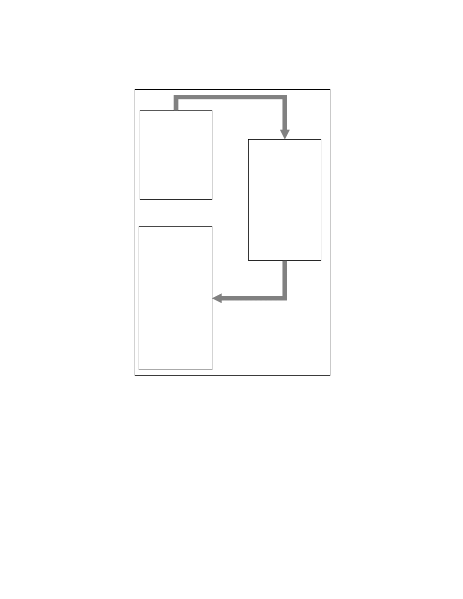
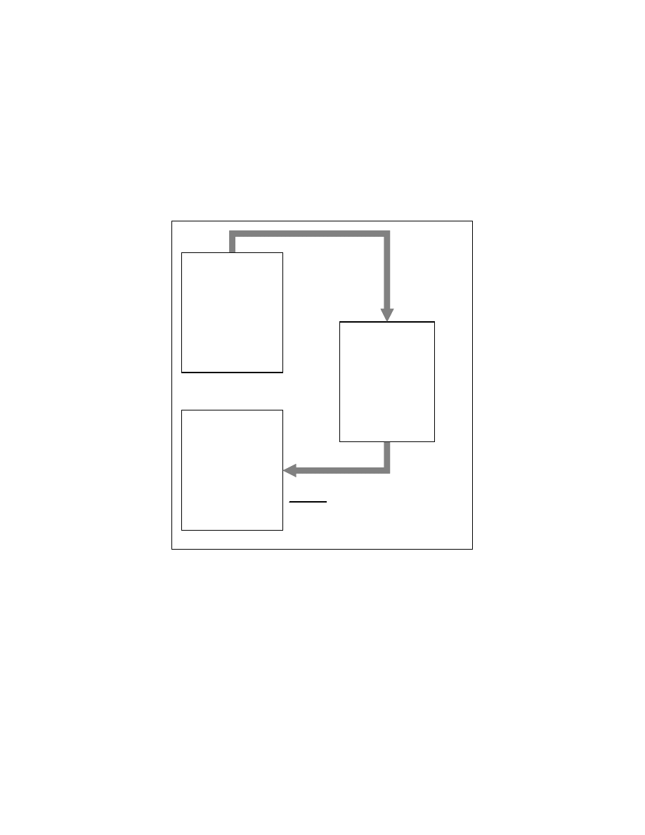
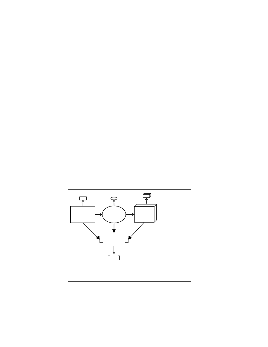
6 Implementation & results
We have implemented a tool, C
⊕, for generating the ZERO form for C programs.
C
⊕ uses the Program Dependence Graph (PDG), generated by the CodeSurfer [5], to
perform the analysis required for imposing an order on the statements of the program.
CodeSurfer provides an API in Scheme [14] to access the PDG representation of the C
programs. The use-def and def-use dependence information is calculated using this PDG
representation. We calculate the def-def dependencies using the CodeSurfer’s defs/kill
sets of the statements. Figure 6-1 shows the architecture of C
⊕.
Partitioning
Engine
CodeSurfer
Dependency
Generator
PT Generator
Ordering
Engine
C
Zero
Form
PDG
PT
PT
DG
Reorderable sets
String Form Generator
Expression AST
String Forms
Figure 6-1: C
⊕ architecture
41
We performed a series of experiments on different sets of C programs to find
study how well our approach imposed order on the statement of the program. The C
programs used in the experiments are listed in Figure 6-2. The Fractal programs [17]
create fractals using C programming language. The COOK system [22] is used for
writing build scripts for projects. It is a powerful and easy to use replacement for make
[18]. Search/Sort programs are the programs that search for data and sort data. We
calculated reorderable percentages, zeroing percentages, and sizes of reorderable sets for
these test programs.
6.1 Reorderable
percentage
We calculated the percentage of program statements that can be reordered by
using the morphing transformation for reordering statements. We call this reorderable
percentage. To calculate this reorderable percentage before the application of zeroing
transformations, we used the following formulae.
Reorderable nodes in PT={n | n
∈PT, ∃n’ ∈ PT and parent (n)=parent (n’) &
reorderable-set-number (n)=reorderable-set-number (n’)} (i.e. the set of nodes that fall in
the reorderable set with size greater than one before application of zeroing
transformations).
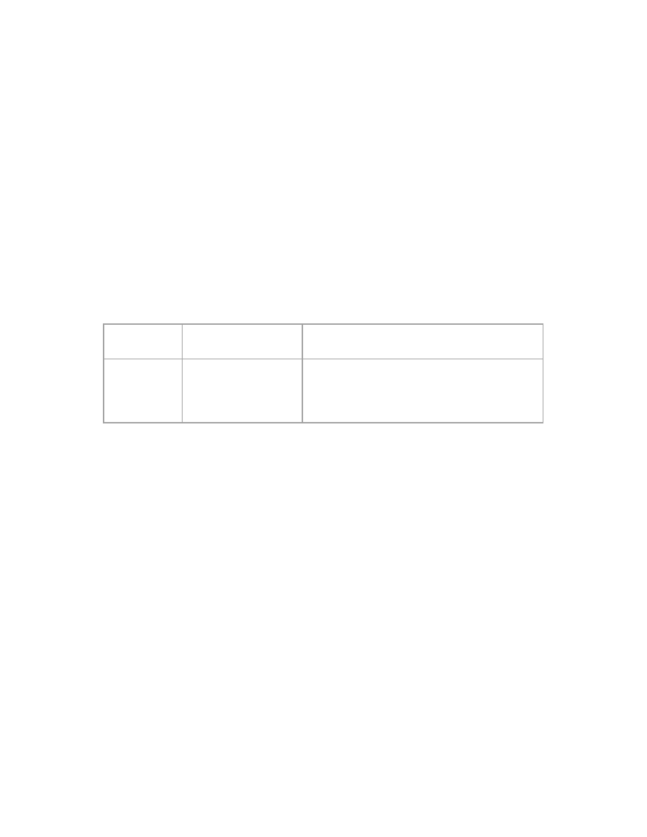
Number
Name
Description
S1
S2
S3
Fractal ( 6 files)
COOK (5 files)
Search & Sort (5
files)
Code for creating fractals
COOK’s project files
Programs to search for data and sort data.
Number
Number
Name
Name
Description
Description
S1
S2
S3
S1
S2
S3
Fractal ( 6 files)
COOK (5 files)
Search & Sort (5
files)
Fractal ( 6 files)
COOK (5 files)
Search & Sort (5
files)
Code for creating fractals
COOK’s project files
Programs to search for data and sort data.
Code for creating fractals
COOK’s project files
Programs to search for data and sort data.
Figure 6-2: Test programs used in C
⊕

42
Percentage of Reorderable nodes = (total number of reorderable nodes in PT *
100) / (total number of nodes in the PT).
After the application of zeroing transformations, reorderable percentage is
calculated using following formulae.
Reorderable nodes in PT={n | n
∈PT, ∃n’ ∈ PT ∋ parent (n)=parent (n’) &
equivalence-class-number (n)=equivalence-class-number (n’) & SR (n)=SR (n’)} (i.e. the
set of nodes that fall in the reorderable set with size greater than one after application of
zeroing transformations).
Reorderable percentage = (total number of failure nodes) *100 / (total number of
nodes in the PT).
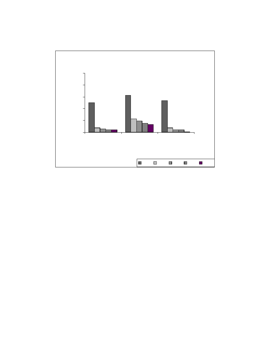
We calculated the reorderable percentages for different string representations.
With the increase in reorderable percentage for a given program, the number of possible
permutations for that program increases. Figure 6-3 shows the reorderable percentages
for our test programs. SR0 corresponds to the reorderable percentage before the
application of zeroing transformations. The Fractal programs have higher reorderable
percentages than COOK system and Search/Sort programs. This is because the Fractal
programs have image processing code that has similar structure of statements that operate
on X and Y coordinates.
43
6.2
Reorderable set sizes
We calculated the sizes of the reorderable sets for the test programs before and
after the application of zeroing transformations on those programs.
The number of reorderable sets with larger size before the appicaltion of zeroing
transformations will be more than the number of reorderable sets with the same size after
application of zeroing transformations. For example, zeroing transformations break
reorderable set of size 25 to two reorderable sets of size 15, and 10 respectively. Ideal
case for zeroing transformations is when the zeroing transformations yield reorderable
sets of size ‘1’ only.
53.8
62.8
49.7
4
19
5
4
15
4
3
13
4
1
13
4
0
20
40
60
80
100
Cook
Fractal
search/sort
Test Systems
Ze
ro
ing Pe
rc
e
n
ta
ge
SR0
SR1
SR2
SR3
SR4
Figure 6-3: Reorderable percentages for the test programs
44
61
24
19
7
2
15
0
2
0
0
0
0
0
6
0
2
0
0
0
0
0
3
0
2
0
0
0
0
0
3
0
2
0
0
0
0
0
2
4
1
0
10
20
30
40
50
60
70
2
3
4
Reorderable set size
N
u
m
b
e
r of
R
e
or
de
ra
bl
e
s
e
ts
SR0 SR1 SR2 SR3 SR4
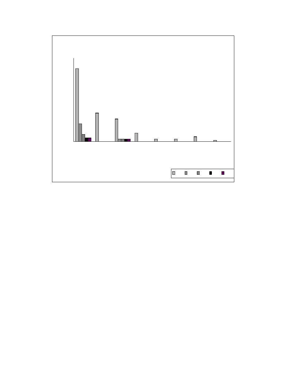
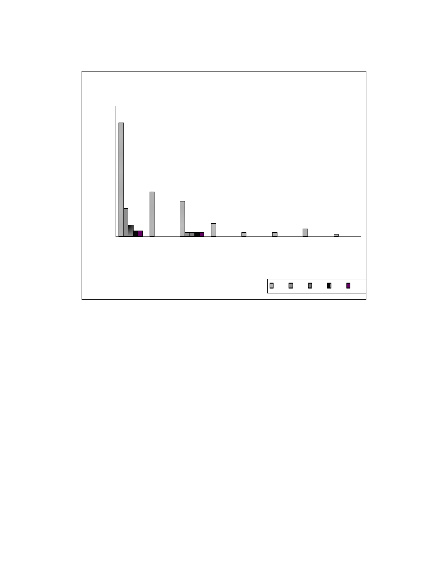
Figure 6-4 plots the sizes of reorderable sets against the number of reorderable
sets with that size for the COOK system before and after application of zeroing
transformations. Reorderable sets with size ‘1’ are not shown in this figure. The aim of
zeroing transformations is to reduce the number of reorderable sets with larger size and
break them into reorderable sets of size ‘1’.
45
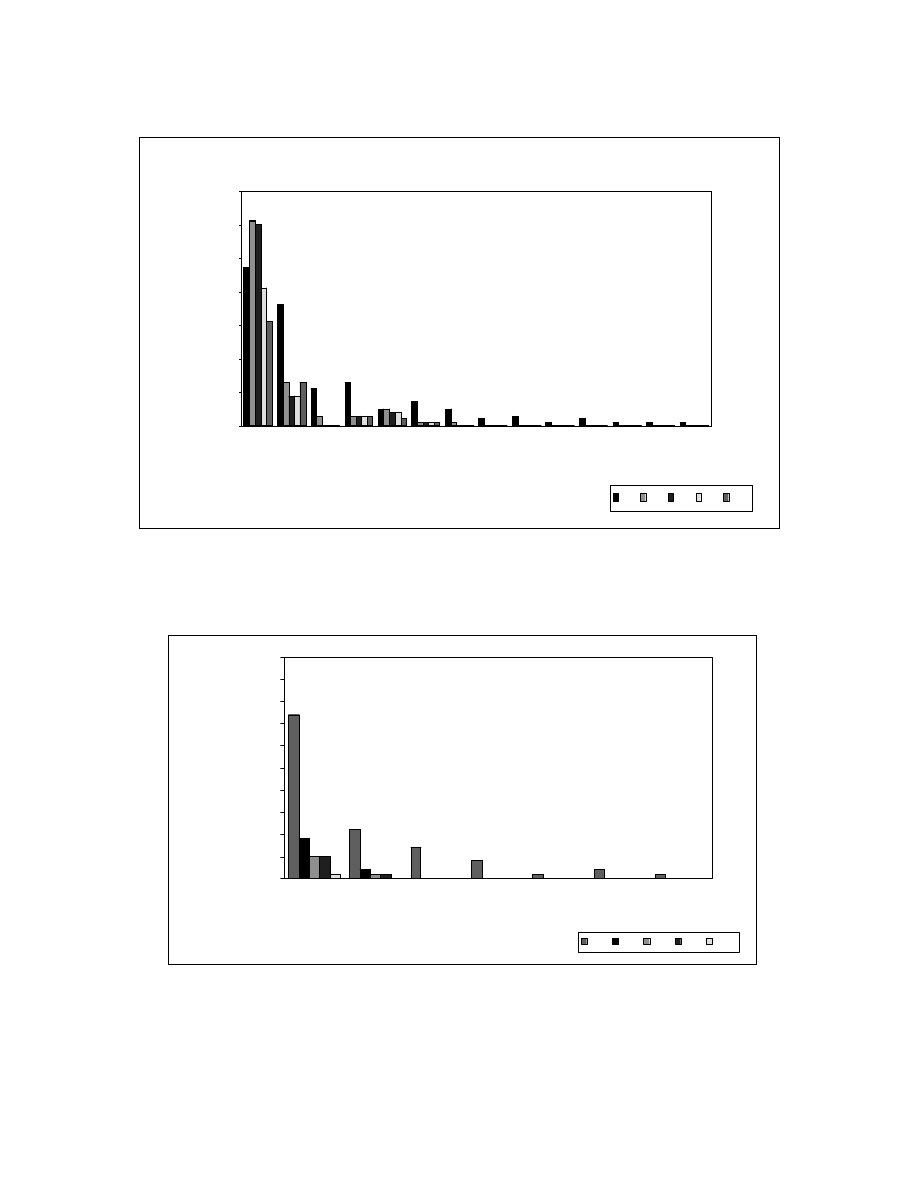
Figure 6-5 and Figure 6-6 show the reorderable set sizes before and after applying
zeroing transformations on Fractal and SEARCH/SORT programs, respectively. The
Fractal programs have reorderable sets of larger sizes when compared to other programs.
This is because the Fractal programs have more dependencies between its statements
when compared to other programs
61
24
19
7
2
15
0
2
0
0
0
0
0
6
0
2
0
0
0
0
0
3
0
2
0
0
0
0
0
3
0
2
0
0
0
0
0
2
4
1
0
10
20
30
40
50
60
70
2
3
4
Reorderable set size
N
u
m
b
e
r of
R
e
or
de
ra
bl
e
s
e
ts
SR0 SR1 SR2 SR3 SR4
Figure 6-4: COOK - Reorderable set sizes
46
47
6160
41
31
36
13
9
13
11
3
13
3333
5544
2
7
1111
5
1
2
3
1
2
1
1
1
0
10
20
30
40
50
60
70
N
u
m
b
er
of
R
eord
er
abl
e
se
ts
2
3
4
5
6
7
8
9
10
11
17
18
20
26
Reorderable set size
SR0 SR1 SR2 SR3 SR4
Figure 6-5: FRACTAL - Reorderable set sizes
37
9
5 5
1
11
2
1 1
7
4
1
2
1
0
5
10
15
20
25
30
35
40
45
50
N
u
m
ber
o
f
R
e
o
rder
abl
e
set
s
2
3
4
5
6
7
8
Reorderable set size
SR0
SR1
SR2
SR3
SR4
Figure 6-6: SEARCH/SORT – Reorderable set sizes
47
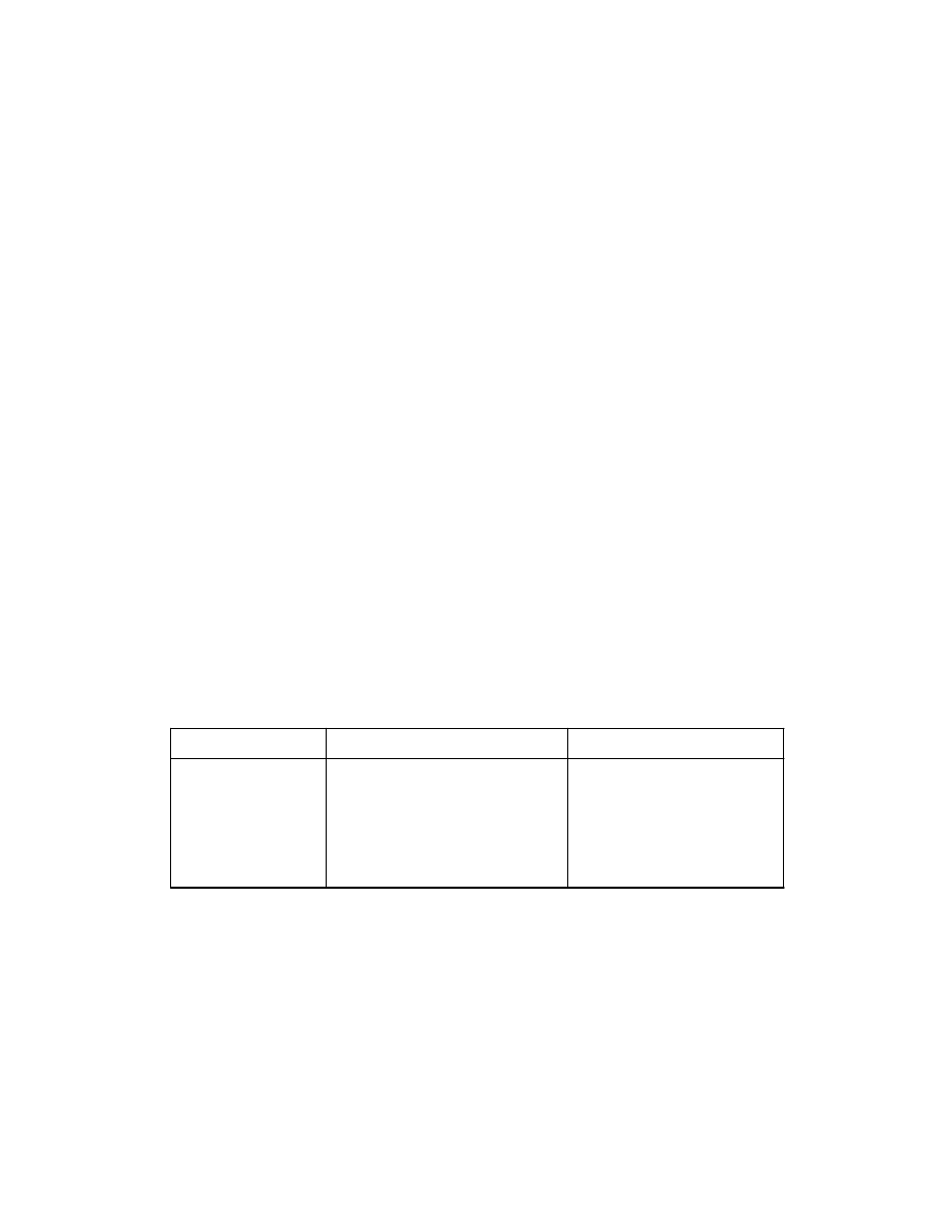
6.3
Number of possible variants
The total number of possible variants of a program that can be generated using
statement-reordering transformation is calculated using the procedure given below.
P = A node in PT
C
1
, C
2
,…, C
n
are children of P.
E
1
, E
2
,…, E
q
are Reorderable sets obtained by partitioning C
1
, C
2
,…, C
n
.
K
1
, K
2
,…, K
q
are sizes of reorderable sets E
1
, E
2
,…, E
q
.
ρ(P) = Total number of permutation obtained by reordering the nodes in the sub-tree
starting with P.
.
1
)
(
.
)).
)
(
(
!
(
)
(
1
nodes
PT
Leaf
P
If
P
nodes
PT
leaf
Non
P
If
E
C
C
K
P
i
j
j
j
i
q
i
−
∈
=
−
−
∈
∈
∋
=
∏
∏
=
ρ
ρ
ρ
The total number of possible permutations for the test programs before and after
applying zeroing transformations is shown in Figure 6-7.
2
1
196787849
Permutations after Zeroing
383968511
78674
1.19 * 10
43
COOK
SEARCH/SORT
Fractal
Permutations before Zeroing
Test System
2
1
196787849
Permutations after Zeroing
383968511
78674
1.19 * 10
43
COOK
SEARCH/SORT
Fractal
Permutations before Zeroing
Test System
Figure 6-7: Number of possible permutations for test programs

7 Conclusions and future work
We have described a method for detecting morphed variants of the viruses. Our
method maps different variants of a virus obtained by morphing transformations to their
respective zero forms. This method may be used to augment the current AV technologies
such as traditional signature scanning approach, and other static and dynamic detection
schemes. AV technologies can use our method to create zero form for a virus and extract
zero signatures of that virus. These zero signatures can be distributed to the users as virus
signatures.
Our method uses zeroing transformations to map different variants of a virus to
zero form. The effectiveness of our method is determined by the effectiveness of zeroing
transformations that map a program to zero form. As our method is a heuristic, we may
not always map all the variants to a single zero form. But the application of zeroing
transformations results in a significant decrease in the number of possible variants of a
program. The experiments we conducted show that, on an average, 55% of the program
statements were reorderable before the application of zeroing transformations which
decreased to 6% after the application of zeroing transformation for fixing the statement
order.
The morphing transformations we consider are dead code insertion, statement
reordering, variable renaming, expression reshaping, and break & join transformations.
In future work, we would like to test our method on actual viruses. We would also
like to do an investigation on other possible morphing transformations and the zeroing
transformations to create zero forms in such cases.

8 Bibliography
[1]
Mihai Christodorescu and Somesh Jha,"Static analysis of executables to detect
malicious patterns," In Proceedings of the 12th USENIX Security Symposium,
Washington, DC, 2003.
[2]
Alfred Aho, Ravi Sethi, and Jeffrey Ullman, Compilers principles, techniques,
and tools, Addison-Wesley, 1986.
[3]
Fredrick Cohen, "Computer viruses-Theory and experiments," Computers and
Security, pp:22-35, 6(1), 1984.
[4]
Jeanne Ferrante, Karl J. Ottenstein, and Joe Warren, "The program dependence
graphs and its use in optimization," ACM Transactions on Programming
Languages and Systems (TOPLAS), pp:319-349, 9(3), 1987.
[5]
GrammaTech, "CodeSurfer - Program analysis tool," 2003
http://www.codesurfer.com
, (last accessed: 08/29/2003).
[6]
Jan Hruska, "Computer virus prevention: a primer," Sophos Labs, 2002
http://www.sophos.com/virusinfo/whitepapers/prevention.html
, (last accessed:
08/29/2003).
[7]
Myles Jordon, "Dealing with metamorphism," Virus Bulletin, pp:4-6, 2002.
[8] Robert
Morgan,
Building an optimizing compiler, Butterworth-Heinemann, 1998.
[9]
Fleming Nielson, Hanne Riis Nielson, and Chris Hankin, Principles of program
analysis, Springer, 1999.
[10] Gabor Szappanos, "Polymorphic macro viruses, part one," Security Focus, 2002
http://online.securityfocus.com/infocus/1635
, (last accessed: 08/29/2003).

50
[11] Péter Ször and Peter Ferrie,"Hunting for metamorphic," In Proceedings of the
11th International Virus Bulletin Conference, pp:521-541, 2001.
[12] Vesselin Bontchev,"Macro and script virus polymorphism," In Proceedings of the
12th International Virus Bulletin Conference, pp:406-438, 2002.
[13] Gabor Szappanos,"Are there any polymorphic macro viruses at all? (… and what
to do with them)," In Proceedings of the 12th International Virus Bulletin
Conference, pp:477-477, 2002.
[14] William Clinger and Jonathan Rees, "Revised report on the algorithmic language
scheme," ACM Lisp Pointers, 4(3), 1991.
[15] Raymond W. Lo, Karl N. Levitt, and Ronald A. Olsson, "MCF: A malicious code
filter," Computers & Security, pp:541-566, 14(6), 1995.
[16] Lawrence M. Bridwell, ICSA Labs 7th Annual computer virus prevalence survey
2001, ICSA Labs, 2001.
[17] Roger T. Stevens, Fractal programming in C, M&T Books, 1989.
[18] Richard M. Stallman, Ronald McGrath, and Paul Smith, "GNU Make, A program
for directing recompilation," 2002.
[19] Symantec, "Understanding heuristics; Symantec's Bloodhound technology," 1997.
[20] VX Heavens, "Virus creation tools," 2002
http://vx.netlux.org/dat/vct.shtml
, (last
accessed: 08/29/2003).
[21] David Moore, Colleen Shannon, and Jeffery Brown,"Code-Red: a case study on
the spread and victims of an Internet worm," In Proceedings of the 2nd Internet
Measurement Workshop, 2002.

51
[22] Chris G. Davis, "Debian cook package," 2003
http://packages.debian.org/stable/devel/cook.html
, (last accessed: 08/29/2003).
[23] David M. Chess and Steve R. White,"An undetectable computer virus," In Virus
Bulletin Conference, 2000.

ABSTRACT
Metamorphic computer viruses programmatically vary their instructions to create
a different form for each infection. This is done using code evolution techniques, such as
introducing dead code, reordering statements, reshaping expressions, and changing
variable names. Current anti-virus technologies use signature, a fixed sequence of bytes
from a sample of a virus, to detect its copies on a user’s machine. Use of signatures does
not work very well with metamorphic viruses since two versions of a metamorphic virus
may have very little in common.
This thesis presents a method to transform different variants of a metamorphic
virus to the same form, called the zero form. Current technologies can be improved to
detect metamorphic viruses by using the zero form of a virus, and not the original
version, for extracting signature. We developed a tool for generating zero forms for C
programs. For the test programs we used, we found that 55% of the statements were
reorderable before applying zeroing transformations for fixing the statement order. After
applying zeroing transformations for fixing the statement order, only 6% of the
statements could not be ordered. The average number of possible permutations of the
program statements obtained by statement reordering transformation reduced from 10
43
to
10
8
with the application of zeroing transformations for fixing the statement order.

Biographical sketch
Mr. Moinuddin Mohammed was born in Rajgaopalpet, India on August 01, 1980.
He graduated with a Bachelor’s degree in Computer Science in June 2001 from Osmania
University, Hyderabad, India. He entered the Master’s program in Computer Science at
the University of Louisiana at Lafayette in Fall 2001. Following completion of this
degree, he will be pursuing a Ph.D. in the area of compilers.
Wyszukiwarka
Podobne podstrony:
Supercompilation for Equivalence Testing in Metamorphic Computer Viruses Detection
Analysis and detection of metamorphic computer viruses
Pairwise alignment of metamorphic computer viruses
Defense In Depth Against Computer Viruses
Detection of metamorphic computer viruses using algebraic specification
Detecting Metamorphic Computer Viruses using Supercompilation
Haisch TOWARD AN INTERSTELLAR MISSION ZEROING IN ON THE ZERO POINT FIELD INERTIA RESONANCE (1996)
Web Sites Hawk Instructions On Making Computer Viruses
Advanced Metamorphic Techniques in Computer Viruses
A Short Course on Computer Viruses
A Model for Detecting the Existence of Unknown Computer Viruses in Real Time
On the Time Complexity of Computer Viruses
Reports of computer viruses on the increase
The Impact of Countermeasure Spreading on the Prevalence of Computer Viruses
The Impact of Countermeasure Propagation on the Prevalence of Computer Viruses
The Asexual Virus Computer Viruses in Feminist Discourse
Mathematical models on computer viruses
The Norman Book on Computer Viruses
An Overview of Computer Viruses in a Research Environment
więcej podobnych podstron