PAIRWISE ALIGNMENT OF METAMORPHIC COMPUTER

VIRUSES

A Writing Project

Presented to

The Faculty of the Department of

Computer Science

San José State University

In Partial Fulfillment

Of the Requirements for the Degree

Master of Science

By

Scott McGhee

December, 2007

© 2007

Scott McGhee

ALL RIGHTS RESERVED

Approved by: Department of Computer Science

College of Science

San José State University

San José, CA

____________________________________

Dr. Mark Stamp

_____________________________________

Dr. David Taylor

_____________________________________

Dr. Teng Moh

Abstract

Computer viruses and other forms of malware pose a threat to virtually any software

system. A computer virus is a piece of software which takes advantage of known

weaknesses in a software system, and usually has the ability to deliver a malicious

payload. A common technique that virus writers use to avoid detection is to enable the

virus to change itself by having some kind of self-modifying code. This kind of virus is

commonly known as a metamorphic virus, and can be particularly difficult to detect [18].

Existing virus detection software is continually being improved upon in order to keep up

with the rising complexity of today’s modern computer viruses. A new approach to

detecting metamorphic viruses, which is an extension of an idea posed in a student

writing project from a previous semester [18], will be considered in this project. If a large

set of viruses in one “family” of metamorphic viruses can be treated as simple sequences

of op-codes, then sequence analysis techniques used in other fields of study like

bioengineering [5] could be used to develop a profile hidden Markov model (HMM).

This profile would then be used to score an arbitrary op-code sequence (i.e. a program

which may or may not be in the virus family) – if the output score exceeds a designated

threshold it could be concluded that the input sequence was likely to have been from that

same virus family.

One of the most common techniques to detect viruses is called signature detection, which

involves an analysis of known viruses to find signatures, or strings of bytes, which are

found in viruses and not in most non-malicious code. If the virus is metamorphic it could

potentially be difficult to find a single signature that will consistently be found in every

version of a metamorphic virus. Since a profile HMM would score the overall similarity

in structure to a virus “family”, it could theoretically detect the virus even if a reliable

signature cannot be created.

In order to develop a profile HMM for a virus family, the first step is to create a multiple

sequence alignment (MSA) for the set of family viruses; this can then be used to “train”

the profile HMM. This paper will concentrate on the techniques for creating MSA’s for

real world virus op-code sequences which will best match the virus family, as well as to

discuss the overall plausibility of the idea of using a profile HMM to detect metamorphic

viruses. Creating and testing the profile HMM to detect the viruses will be the subject of

another student project.

7

Table of Contents

1

Introduction................................................................................................................ 10

2

Computer Viruses ...................................................................................................... 11

2.1

Encrypted Viruses............................................................................................. 12

2.2

Polymorphic viruses.......................................................................................... 13

2.3

Metamorphic Viruses........................................................................................ 13

3

Existing Virus Detection Methods............................................................................. 16

3.1

Code Emulation ................................................................................................ 16

3.2

Pattern based scanning...................................................................................... 16

3.3

Heuristic Analysis............................................................................................. 17

3.4

Using Hidden Markov Models.......................................................................... 18

3.5

Proposed Strategy: Using Profile Hidden Markov Models .............................. 19

4

Op-Code Sequence Definitions ................................................................................. 20

5

Virus Alphabet Definition / Conversion.................................................................... 21

6

Pairwise Alignment ................................................................................................... 23

6.1

Mutational Processes ........................................................................................ 24

6.2

Permutation Affects on Alignments.................................................................. 25

6.3

Op-code Sequence Preprocessing ..................................................................... 26

6.3.1 Exhaustive Search......................................................................................... 27

6.3.2 Subroutine Matching..................................................................................... 27

6.4

Alignment Scoring............................................................................................ 28

6.4.1 Substitution Matrices .................................................................................... 29

6.4.2 Gap Penalties ................................................................................................ 31

6.5

Pairwise Alignment Using Dynamic Programming ......................................... 33

6.5.1 Reconstructing the Alignment ...................................................................... 35

6.5.2 Algorithm Efficiency .................................................................................... 35

7

Multiple Sequence Alignment ................................................................................... 36

7.1

Progressive Alignment Algorithm .................................................................... 37

7.1.1 Choosing Alignments.................................................................................... 39

7.1.2 Example Multiple Alignment ....................................................................... 40

8

7.1.3 Ordering Alignment Insertions ..................................................................... 43

7.1.4 Algorithm Efficiency .................................................................................... 46

7.2

Determining Alignment Quality ....................................................................... 47

7.3

Case Study: NGVCK Virus Alignment ............................................................ 48

7.4

Case Study: VCL32 and PS-MPC Virus Alignments....................................... 53

8

Preliminary Profile HMM Results............................................................................. 55

9

Future Research Needed ............................................................................................ 56

9.1

Scoring Refinement .......................................................................................... 56

9.2

Affects of Preprocessing on a Profile HMM .................................................... 57

10 Conclusion ................................................................................................................. 58

11 References.................................................................................................................. 59

9

Table of Figures

Figure 1: Op-code to symbol lookup table ..............................................................................22

Figure 2: Sample virus from NGVCK .....................................................................................23

Figure 3: Alignment for the first part of two NGVCK Virus Subroutines ..............................24

Figure 4: Effects of Permutation on Standard Alignments......................................................25

Figure 5: BLOSUM 50 substitution matrix .............................................................................30

Figure 6: Initial Op-code Substitution Matrix with values given for relative scores...............30

Figure 7: Gap Penalty Graphs..................................................................................................32

Figure 8: Minimum-Spanning Tree for adding Alignments ....................................................41

Figure 9: Snapshot of 3

rd

iteration in the progressive MSA algorithm....................................42

Figure 10: Example ordering for each of the four chosen insertion sequences .......................44

Figure 11: Sub-trees given in a spanning forest created after inserting the 6

th

edge ...............45

Figure 12: Score Distributions for both NGVCK test sets with sample size 780....................50

Figure 13: Conservation percentage based on group size for NGVCK...................................51

Figure 14: Graphical representation of groups of 20 preprocessed NGVCK viruses..............52

Figure 15: Graphical representation of groups of 20 raw NGVCK viruses ............................52

Figure 16: Score distributions for VCL32, PS-MPC, and NGVCK (Preprocessed) ...............54

Figure 17: Conservation Percentage of VCL32, PS-MPC, and NGVCK (Preprocessed).......54

Figure 18: Graphical representation of MSA’s created for PS-MPC and VCL32 ..................55

10

1 Introduction

In today’s world, computers have become integrated into the fabric of our society, so

much so that the potential for disaster exists if a critical system or group of systems were

to somehow malfunction or be corrupted. Computer viruses and other forms of malware

pose a threat to virtually any software system, and because of this they are a threat to our

way of life. Computer viruses take advantage of an inherent weakness to deliver some

kind of malicious payload by performing an action or sequence of actions which can do

some harm. In some cases the payload could be relatively harmless, but in other cases the

payload can be devastating to the system. After infection, many viruses will attempt to

spread to another system usually by the same means in which the system was originally

infected, or in some cases there can be several ways the virus will spread to other

systems. Often times this kind of malicious software is referred to as a “worm” or in

some cases “malware,” but in this paper the generic term “virus” will be used to refer to

this broad category of software.

One kind of virus which is generally believed to be difficult to detect is a metamorphic

virus. This kind of virus has the ability to change its internal structure ensuring any two

instances of the same virus will likely be different from each other, even though they will

behave the same. Metamorphic viruses will be described in more detail later. Depending

on the degree of metamorphism, some of the existing methods of detection, which rely to

some extent on the internal structure of the virus, have a difficult time dealing with this

kind of virus [18].

11

The purpose of this paper is to explore a new approach for detecting metamorphic viruses

which involves some of the same techniques currently used in bioinformatics to analyze

protein and DNA sequences. It is important to note that an individual virus can be

represented as a sequence of op-codes or processor instructions (assuming the virus can

be decompiled), which is analogous to a DNA sequence (or a gene) which can be

represented as a sequence of letters (each letter being a base pair in a DNA molecule).

The idea behind this new approach is that similar algorithms used by bioengineers to

determine if a protein sequence is part of a particular family can be used to determine if

an op-code sequence is part of a metamorphic virus family. The metamorphic virus is

referred to as a family because, similar to a protein family, there can be potentially

limitless versions of the virus, all of which are related.

This new approach is an extension to research done in [18] which explored the use of a

hidden Markov Model (HMM) to detect metamorphic viruses. The approach presented in

this paper will use a profile HMM instead, which is based on multiple alignments created

for op-code sequences. This paper will concentrate on the problem of creating the

alignments for virus op-code sequences – the profile HMM itself will only be briefly

introduced in this paper and is the main focus of another student research.

2 Computer Viruses

There are many kinds of viruses, all of which can have many different ways of causing

damage. Usually there are ways for virus detection software to detect the virus before it

can get a chance to deliver any kind of payload. In the following subsections common

12

techniques virus writers use to avoid detection will be presented along with some of their

associated strengths and weaknesses.

2.1

Encrypted Viruses

One technique commonly used by virus writers is to ensure that a large portion of the

binary form of the virus on disk is encrypted, except for a small segment of code which

can decrypt the virus when it is executed. Although the virus itself never changes, the key

used to encrypt and decrypt the virus will be different for every generation of the virus. In

this way, when the virus is stored on disk it will always be encrypted, the only time the

unencrypted form is visible would be when the virus has decrypted itself in memory.

This kind of virus has two major weaknesses:

 The small segment of code which decrypts the virus never changes on disk and

thus can be detected

 A software emulator could be used to simulate the virus and then gain access to

its decrypted form of the virus. Since the virus itself never changes, it is then open

to detection.

Detection of such viruses is still possible without trying to decrypt the actual virus body.

In most cases the code pattern of the decryptor of these viruses is unique enough for

detection [13]

13

2.2

Polymorphic viruses

Polymorphic viruses are a special form of encrypted viruses which uses the same basic

principle the addition that the decryptor will not be the same in every generation of the

virus. This kind of virus has the ability to change or to swap the decryptor with a different

version each time the virus spreads. Usually a polymorphic virus will have a large

number of possible decryptors making it difficult to detect the decrypter portion of the

virus alone. Win32/Marburg and Win95/HPS were the first viruses that used real 32-bit

polymorphic engines. Polymorphic viruses can create an endless number of new

decryptors that use different encryption methods to encrypt the constant part of the virus

body [13]. The unencrypted form of the virus body will still remain static from one

generation of the virus to the next, which means that this kind of virus is still susceptible

to detection when the virus is emulated.

2.3

Metamorphic Viruses

The major flaw in both encrypted and polymorphic viruses is that while the unencrypted

form of the virus body may be difficult to retrieve, the virus body itself always remains

the same. This means that usually encrypted or polymorphic viruses can be detected

assuming the detection software is advanced enough to obtain the unencrypted form of

the virus. A metamorphic virus, on the other hand, is a type of virus which can contain

variations in the virus body itself. This kind of virus usually involves an assembly

mutation engine of some kind, in which the disassembled virus is altered in such a way

that when the virus is reassembled it will look different than the original virus even

though it still behaves the same as the original. The amount of differentiation this

14

mutation can provide depends on the complexity of the engine used. The following are

examples of the different kinds mutations which are often used inside of common

engines:

 Random reordering of the subroutines

 Insertion or removal of Junk code (code with no affect to behavior)

 Instruction substitutions: where sequences of instructions can be substituted for a

different but equivalent set of instructions.

The following is an example of a simple substitution mutation for a segment of assembly

code taken from [8]:

XOR Reg,-1

—> NOT Reg

SUB Mem,Imm

—> ADD Mem,-Imm

XOR Reg,0

—> MOV Reg,0

ADD Reg,0

—> NOP

AND Mem,0

—> MOV Mem,0

XOR Reg,Reg

—> MOV Reg,0

SUB Reg,Reg

—> MOV Reg,0

AND Reg,Reg

—> CMP Reg,0

TEST Reg,Reg

—> CMP Reg,0

LEA Reg,[Imm]

—> MOV Reg,Imm

MOV Mem,Mem

—> NOP

Also in [9] there are many instruction substitutions that were meant for optimizing

assembly code – the following table gives just a few examples.

Instruction

CPU’s

Replacement or
action

Description / Notes

or reg, reg

Pent

test reg, reg

Better pairing
because OR writes
to register. (This is
for src = dest.)

15

pop mem

486+

pop reg
mov mem, reg

Faster on 486+
Better pairing on
Pentium

push mem

486+

mov reg, mem
push reg

Faster on 486+
Better pairing on
Pentium

In some cases the virus can be packaged with this mutation engine, so that the virus itself

has this ability to mutate its own assembly; however, in an attempt to make the virus

more light-weight the virus writer could create a virus generator which uses the engine to

create many versions of the virus up-front and then send them out independently of each

other.

The example viruses studied in this paper are all the result of virus generators which are

commonly found on the internet. The following viruses are studied in this paper and were

taken from VX Heavens search engine [15]:

 NGVCK (Next Generation Virus Generation Kit)

 VCL32 (Virus Creation Lab for Windows 32)

 PS-MPC (Phalcon/Skism Mass-Produced Code Generator).

Even though viruses created by a generator usually do not self-modify from one

generation to the next, virus detection software will need to detect each version of the

virus independently in order to be effective. Because of this, the problem of detecting the

output of a virus generator will not be distinguished from the problem of detecting a self-

modifying metamorphic virus.

16

3 Existing Virus Detection Methods

There are many different technologies available to detect viruses most of which rely on

the internal structure (rather than the behavior) of the virus. Although the behavior of

each of the permutations of a metamorphic virus is the same, the structure is different

which means they can become difficult to detect depending on the amount of variation.

There are some detection methods which detect suspicious ability or behavior within a

program, such as heuristic analysis; however these methods are rarely used as a sole

means of virus protection as they are normally prone to false-positives [18]. The

following subsections will discuss various existing methods, as well as outline the

proposed strategy to use profile HMMs for detection.

3.1

Code Emulation

Code emulation was briefly mentioned when discussing encrypted and polymorphic

viruses as a possible means of retrieving the unencrypted form of the virus body. Using

code emulation can be an effective tool when detecting viruses, since it involves

emulating software on a virtual machine rather than a real processor [18]. Because the

virus is in a controlled environment, the system emulating the virus will not run any risk

of harmful side-effects of the virus.

3.2

Pattern based scanning

One of the most common approaches to detecting viruses is called string or signature

scanning. At a high level, signature scanning involves a set of signatures, or a string of

bytes which can contain wild cards, which are found in viruses but not found in non-

17

malicious code. These signatures often contain non-contiguous code, using wild cards

where differences lie. These wild cards allow the scanner to detect if virus code is padded

with other junk code [6]. This kind of detection requires research on known viruses, and

patterns within each virus need to be studied so that these signatures can be found.

Although signature scanning works well on most viruses, a metamorphic virus could

potentially create enough variation within the application making it nearly impossible to

create a reliable signature.

3.3

Heuristic Analysis

Heuristic programming is usually regarded as an application of artificial intelligence, and

as a tool for problem solving. In a sense, heuristic anti-malware attempts to apply the

processes of human analysis to an object [10]. Some of the more common heuristic

scanning mechanisms will search for suspicious instruction sequences.

For example the following are considered suspicious by a common heuristic scanner

called TbScan [14]

 Suspicious file access. Might be able to infect a file.
 Relocator. Program code will be relocated in a suspicious way.
 Suspicious Memory Allocation. The program uses a non-standard way to search

for, and/or allocate memory.

 Wrong name extension. Extension conflicts with program structure.
 Contains a routine to search for executable (.COM or .EXE) files.
 Found an instruction decryption routine. This is common for viruses but also for

some protected software.

 Flexible Entry-point. The code seems to be designed to be linked on any location

within an executable file. Common for viruses.

18

 The program traps the loading of software. Might be a virus that intercepts

program load to infect the software.

 Disk write access. The program writes to disk without using DOS.
 Memory resident code. This program is designed to stay in memory.
 Invalid opcode (non-8088 instructions) or out-of-range branch.
 Incorrect timestamp. Some viruses use this to mark infected files.
 Suspicious jump construct. Entry point via chained or indirect jumps. This is

unusual for normal software but common for viruses.

 Inconsistent exe-header. Might be a virus but can also be a bug.
 Garbage instructions. Contains code that seems to have no purpose other than

encryption or avoiding recognition by virus scanners.

 Undocumented interrupt/DOS call. The program might be just tricky but can also

be a virus using a non-standard way to detect itself.

 EXE/COM determination. The program tries to check whether a file is a COM or

EXE file. Viruses need to do this to infect a program.

 Found code that can be used to overwrite/move a program in memory.
 Back to entry point. Contains code to re-start the program after modifications at

the entry-point are made. Very common for viruses.

 Unusual stack. The program has a suspicious stack or an odd stack.

3.4

Using Hidden Markov Models

A new more experimental approach to detecting metamorphic viruses is explored in [18]

and involves the use of a hidden Markov model (HMM). An HMM is defined as a

statistical model in which the system being modeled is assumed to be a Markov process

with unknown parameters, and the challenge is to determine the hidden parameters from

the observable parameters [16].

19

In this case the system being modeled is a family of metamorphic viruses, and the

observable parameters are the op-codes within the disassembled viruses. The amount and

meaning of the hidden parameters is unknown. To begin with, the number of hidden

parameters is simply guessed and an initial HMM with arbitrarily chosen transition

probabilities is created. Afterwards the HMM is progressively “trained” on particular

dataset of op-code sequences, the resulting HMM can be used to score an arbitrary input

sequence. If the score is over a designated threshold, then it can be concluded that the

input sequence is part of the virus family for which the HMM was trained.

In [18], an HMM is created for some viruses created by a common virus generator, the

Next Generation Virus Creation Kit (NGVCK). The possibility of using hidden Markov

models showed some promise as it was able to successfully detect the NGVCK virus

family with a high success rate and low false-positive rate.

3.5

Proposed Strategy: Using Profile Hidden Markov Models

The approach which is proposed in this paper will be to use a profile hidden Markov

model (HMM) to detect metamorphic viruses. The overall approach will be split into two

individual pieces: the first piece involves creating a multiple sequence alignment (MSA)

for a predefined set of metamorphic viruses in the same family, and the second piece will

use the MSA created in the first part to train a profile HMM and test to find the resulting

scores on various virus and non-virus sequences. Similar to the approach with a standard

HMM, if the resulting score from the profile HMM is over a designated threshold then it

can be concluded that the input sequence was part of the virus family which was used to

create the MSA.

20

This paper will concentrate on the first piece of problem: to create high quality MSA for

a set of computer virus op-code sequences. The second piece of the problem, creating and

testing the profile HMM using an MSA, is the main topic of discussion in another student

project [2].

Although this approach is similar to the use of a standard HMM, a profile HMM will use

position specific information within the alignment for scoring [1], which should prove to

be an advantage. When an input sequence is scored by a profile HMM, it will score

higher if it is structurally similar to the alignment which was used to train the profile

HMM. In contrast, a standard HMM scores an input sequence based purely on symbol

transition statistics and does not use information about the overall structure of the code

when calculating scores.

4 Op-Code Sequence Definitions

The types of sequences analyzed in this paper will be finite ordered lists of symbols from

an alphabet with a finite set of available symbols. In the field of natural science, a

sequence of residues found in protein molecules can be expressed as a sequence of letters

from the English alphabet (A – Z) in which each letter stands for a unique residue [5]. In

this paper, a similar approach to represent viruses will be taken. Essentially a virus is

made up of a sequence of op-codes or processor instructions which can be taken from the

disassembled version of the virus. Instead of taking the entire instruction (which can

include an instruction, offsets, data, and processor registers), only the high level

instructions will be considered, the rest will be ignored.

21

For simplicity of the display of a single op-code as a single character, only the top 36

most commonly used op-codes will be considered. These will be represented as letters

from the English alphabet [A-Z] and single numerical digits [0-9], all other op-codes will

be represented as an asterisk ‘*’. Although this does limit the number of unique op-codes

that can be expressed in an op-code sequence, the top 14 op-codes account for

approximately 90% of all instructions used in any typical program [3]. In addition, the

top 36 op-codes accounted for approximately 99.3% of all op-codes found in sequences

which were analyzed in this paper.

Special characters for divisions in the decompiled version of the virus will also be

provided in the alphabet. A bar ‘|’ character will be used to represent the start of a

subroutine, and a semi-colon ‘;’ character will be used to represent the start or the end of

a block of instructions - both of which can be uniquely identified in the output from IDA

Pro [4]. These special symbols will be referred to as a ‘marker’ in an op-code sequence.

The markers will be used to ensure that subroutines will be aligned properly together with

the assumption that these blocks are inherently important to the internal program

structure of the program.

5 Virus Alphabet Definition / Conversion

In order to easily display and align a disassembled application, a table in Figure 1 is

presented with all the available symbols used in the op-code sequences which are

analyzed in this paper. The symbols are ordered by frequency where the symbol ‘A’ is

the most frequent and ‘9' is the least frequent. The * will represent the rarer symbols

which do not appear very often in the test sets. Using this symbol lookup, a simple

22

parsing algorithm was used to extract the op-codes used in the raw disassembled viruses

from IDA Pro.

An example of this conversion is given in Figure 2 where a small section of the

disassembled file is given, as well as the converted op-code sequence with the related

section for the subroutine underlined. The parsing algorithm used simple java string

regular expressions to identify on each line if the line contained one of the supported op-

codes or markers.

The disassembled subroutine and the op-code sequence presented in Figure 2 were taken

from a set of NGVCK (Next Generation Virus Creation Kit) viruses. There will be

Op-Code

Rep

Op-Code

Rep

Op-Code

Rep

Op-Code

Rep

ÄÄÄÄ

;

jb

Q

xchg

7

Bound

*

ÛÛÛÛ

|

or

R

ja

8

js

*

mov

A

shl

S

sbb

9

jp

*

add

B

clc

T

sar

*

fild

*

push

C

test

U

stosd

*

fld

*

pop

D

stc

V

rcr

*

scasb

*

call

E

not

W

rep

*

aad

*

sub

F

adc

X

lodsw

*

enter

*

cmp

G

rcl

Y

stosw

*

cmc

*

jz

H

cld

Z

lodsd

*

jns

*

retn

I

neg

0

stosb

*

jno

*

jnz

J

ror

1

lodsb

*

jecxz

*

jmp

K

shr

2

loop

*

hlt

*

dec

L

rol

3

in

*

icebp

*

xor

M

imul

4

retf

*

jle

*

inc

N

div

5

std

*

fnstenv

*

lea

O

jnb

6

jnp

*

out

*

and

P

Figure 1. Op-code to symbol lookup table

23

several references to this particular virus set to demonstrate various concepts, more detail

surrounding this virus and results of tests performed on the virus will be presented in the

NGVCK Case Study (Section 7.3).

(a)

; ÛÛÛÛÛÛÛÛÛÛÛÛÛÛÛ S U B R O U T I N E ÛÛÛÛÛÛÛÛÛÛÛÛÛÛÛÛÛÛÛÛÛÛÛÛÛÛÛÛÛÛÛÛ
sub_4013D4

proc near

; CODE XREF: sub_4013EC_p sub_401408_p

pusha
lea

ebx, (dword_40103A+0D3h)[ebp]

push

114h

pop

edx

loc_4013E1:

; CODE XREF: sub_4013D4+14_j

mov

byte ptr [ebx],

0

sub

ebx, 0FFFFFFFFh

dec

edx

jnz

short loc_4013E1

popa
retn

sub_4013D4

endp

; ÛÛÛÛÛÛÛÛÛÛÛÛÛÛÛ S U B R O U T I N E ÛÛÛÛÛÛÛÛÛÛÛÛÛÛÛÛÛÛÛÛÛÛÛÛÛÛÛÛÛÛÛÛ

(b)

;EDFACDRHCODA0WALBGJ;;NLFAAFAFABMAAAA2*6MMLJMMLJWWA3AADI;AM
BBBABNBAABNBAAMBAAOOELFBAAFBBFJK;CDCDRHASBK;AFCEAABENHEGHEG
JLACEK

|COCDAFLJDI|

EABCCEAI|EABCPBCEI|EQAAMHK;GJK;AG8BGHMHGH

APGHAXPGJEQEI;ACDCD2SAFGHAGHFMLK;BAB7B7GHK;BFAPGHK;NFAAOCI|
CFAPAA5FABADI|AABBAFCDBAAEA0ACEDAEQAABCDBALF4BBASBAAAAFBABC
CDBBFAAACCBDAEAFBABDBABABABRADOAB*A*W0*FJABNFATI;VI|CCXCCCA

CABCENHLA|CDCFCCCCCCEADBAGHCCCCCEUHAATI|ECNEVI|CECEI|CAAAAB
PBABAAZEAFUHAAABLNMGJK;AASBAMASBABADI;DDK

Figure 2. Sample virus from NGVCK, (a) The raw decompiled subroutine; all op-

codes/markers that contain a symbol in the alphabet are underlined and

italicized, (b) The full op-code sequence for the NGVCK virus, with the related

subroutine in (a) underlined and italicized.

6 Pairwise Alignment

In order for the proposed method to detect metamorphic viruses to work, first we must

define an effective means of aligning a pair of op-code sequences. An alignment can be

created for any pair of sequences, although usually it is created for similar (or related)

sequences. Obviously, sequences that are exactly the same do not require an alignment,

24

since these sequences are already aligned. To visualize the alignment, the sequences can

be considered rows in a matrix, and the symbols are individual columns. All symbols in

one sequence will then be aligned with symbols in the other sequence so that related

symbols or subsequences will align to the same column. In order to accomplish this, gaps

can be inserted into either sequence, in which a gap is simply a special character usually

represented by a ‘–’ (dash).

In the example in Figure 3, the output from the prototype op-code alignment program

shows an alignment of two op-code sequences representing one subroutine.

(a)

Unaligned Sequences:

|AABNBAFCDBAAEAABCEDAEQCDABABBAF4NBBMBTYBAAAAABBCD
|AABBAFCDBAAEA0ACEDAEQAABCDBALF4BBASBAAAAFBABCCD

(c)

Alignment With Gaps:

|AABNBAFCDBAAEA-ABCEDAEQCD-ABABBA-F4NBBMBTY--BAAAA--ABB-CD
|AAB-BAFCDBAAEA0A-CEDAEQ--AABCDBALF4-BB----ASBAAAAFBAB-CCD

Figure 3. Alignment of the first part of two NGVCK Virus Subroutines

The alignment created here shows that there are many small matched sequences of length

3 to 10. The algorithm used to generate this alignment will be discussed later, but for now

it will be sufficient to assume that the alignment in Figure 3 will be fairly typical for

viruses which are metamorphic.

6.1

Mutational Processes

When comparing two sequences, one of the purposes of using an alignment is to look for

evidence that the sequences diverged from a common ancestor by a process of mutation

25

and selection [5]. In the case of proteins and DNA sequences, the basic mutational

processes which are normally considered are the following:

 Substitutions – a subsequence in the original is substituted for a new subsequence

 Insertions – the subsequence was inserted into the original

 Deletions – the subsequence was removed from the original

In the case of metamorphic viruses, these kinds of processes can also occur; however,

there is another basic process which would not normally be found in biological

sequences:

 Permutation – a random re-ordering of the original sequence

A permutation could technically be stated in terms of a series of insertions and deletions,

however it is important to make a distinction between these two mutational processes

since a permutation is not a random series of insertions and deletions.

6.2

Permutation Affects on Alignments

Knowing that highly metamorphic viruses may use permutation in its alignments, it is

important to recognize the impact which permutation can have on pairwise alignments. It

is easy to see that even a very simple permutation can have a large affect.

ABCDEFGHIJKLMNOPQRSTUVWXYZ-------------

-------------NOPQRSTUVWXYZABCDEFGHIJKLM

26

Figure 4. Effects of Permutation on Standard Alignments

As an example to demonstrate this, a simple permutation to take the second half of a

sequence and placing it in the beginning is given in Figure 4 with the resulting pairwise

alignment. By extension, it is easy to see how a more complex permutation, such as

reversing the sequence or randomizing the symbols, will greatly reduce the quality of

simple pairwise alignments.

6.3

Op-code Sequence Preprocessing

In order to cope with the problem which permutation causes alignments, it may be

possible to preprocess the sequences being aligned in such a way that any permutations

which may have occurred are reversed. This preprocessing step could be the key to

creating a high quality alignment for metamorphic virus op-code sequences; however, it

is important that the preprocessing step will preserve as much of the structure in the

sequences so that alignments created will still score low if the sequences being aligned

are not related.

In order to preserve the structure of the op-code sequence, rules which the preprocessing

transformations must follow must be defined. The initial version of this preprocessing

step will only allow reordering of subroutines/blocks within the op-code sequences, or

more precisely:

 Subsequences within blocks or subroutines cannot be changed

 No insertions or deletions can be performed, only permutation is allowed

27

Within these constraints, the problem then becomes how can the blocks or subroutines be

permuted to ‘reverse’ any previous permutations.

In the following subsections, the term “target sequence” will be used to refer to the

sequence being preprocessed, and the term “source sequence” will be used to refer to the

sequence which the target sequence is being permuted to match.

6.3.1 Exhaustive Search

The most obvious solution, and the easiest to implement, is an exhaustive search over all

possible permutations of the target sequence. This search will simply choose the

permutation of the target sequences which generates the highest scoring alignment with

the source sequence. The results from this search will guarantee the best possible result.

The issue with this approach is that the time complexity increases exponentially on the

number of subroutines in the target sequence. If the time it takes to complete the

algorithm was of no concern, either because the number of subroutines was small enough

or for any other reason, then an exhaustive search is a viable option.

6.3.2 Subroutine Matching

Another simple solution which will produce good results is to attempt to match up all

subroutines in the source sequence with subroutines in the target.

Subroutine Matching Algorithm Specification

S = list of subroutines in the source

T = list of subroutines in the target

O = output list of subroutines

28

For each subroutine s in S

Find t

 T with the highest alignment score with s

Add t to O, remove t from T

Add any remaining subroutines in T to O

This algorithm is fairly simple and only has a polynomial time complexity O(n

2

) on the

number of subroutines. The issue with the algorithm as stated above is that because the

search is performed in sequential order by the subroutines in the source, it is possible that

a sequence from the target which had a much higher score aligning with a later

subroutine in the source will be chosen accidentally.

To fix this a small enhancement can be made to first align all pairs of subroutines in S

and T, and then attempt to match sequences in S with sequences in T in the order of

sequences which have the highest scoring alignments. This enhancement adds an

additional polynomial factor to the time complexity of the algorithm, but will increase the

effectiveness of the matching.

6.4

Alignment Scoring

When creating an alignment for an arbitrary pair of sequences, the first step is to define

how an alignment will be scored. The score will determine how likely the alignment was

made because the sequences were related (a high score), or if the alignment was just

random (a low score). Any two sequences with enough symbols (for example ten or

more) will have many different possible alignments which can be created, however when

a scoring model is defined there will usually be only one alignment which maximizes the

score. It is possible, depending on the constraints of the scoring model, that two or more

29

alignments will all have the same maximum score, in which case it is sufficient to

randomly choose one alignment to be the sole maximum [5]. In a pairwise alignment,

symbols can either be matched with another symbol (a substitution) or there can be a gap

inserted – this means to properly score a pairwise alignment a substitution scoring matrix

in combination with a gap penalty model can be used.

6.4.1 Substitution Matrices

One of the most important activities which must take place in order to come up with a

proper scoring model which will result in the best possible alignments is to come up with

a substitution scoring matrix. This matrix will have all the score values used when a

symbol is aligned with any other symbol. This means that if a given sequence uses an

alphabet which has 100 symbols, the scoring matrix will need to be 100 x 100 in size. It

is important to note that a substitution matrix will have the following properties:

 Values on the diagonal are substituting a symbol with the same symbol, and in

general these values will be the highest number in the column.

 A scoring matrix will be reflective – on scoring matrix M,  i, j

ji

ij

M

M



In the matrix in Figure 5, the BLOSUM 50 substitution matrix for protein residues shows

that substituting a residue ‘R’ with the residue ‘D’ will be given a score -2, whereas

replacing an ‘R’ with the same symbol ‘R’ will give s core of +7. This matrix is the

product of extensive research and computation on large databases of aligned, un-gapped

protein sequences [5].

30

A

R

N

D

C

Q



A

5

-2

-1

-2

-1

-1



R

-2

7

-1

-2

-4

1



N

-1

-1

7

2

-2

0



D

-2

-2

2

8

-4

0



C

-1

-4

-2

-4

13

-3



Q

-1

1

0

0

-3

7



















Figure 5. BLOSUM 50 substitution matrix. Some of the matrix has not been given,

and values on the diagonal have been bolded.

We will now need to come up with a similar substitution matrix which will apply to op-

codes instead of protein residues. In order to do this, some initial criteria can be made to

take an initial guess for the values. When more research is done for likely op-code

substitutions, the criteria and actual values in the matrix can be further refined (see

Section 8.2). In Figure 6 the initial scoring matrix used in this paper is presented.

;

|

A

B



9

*

;

2

2

-20

-20



-20

-20

|

2

2

-20

-20



-20

-20

A

-20

-20

2

-1



-1

-1

B

-20

-20

-1

2



-1

-1

















9

-20

-20

-1

-1



2

-1

*

-20

-20

-1

-1



-1

6

Figure 6. Initial Op-code Substitution Matrix with values given for relative scores

The following was the criteria for used to fill in the matrix:

 matching two symbols that are exactly the same is a positive score

 matching two ‘rare’ symbols with each other is a medium positive score

 matching two different symbols is a low negative score

 matching two markers is a low positive score

31

 matching a marker with a non-marker is a high negative score

6.4.2 Gap Penalties

In an ideal alignment, each symbol from the first sequence should have a one to one

relationship with symbols in the second. This will likely be too much to ask in even the

most highly related sequences. So gaps must be allowed in the alignment, which usually

means a penalty on the score of that alignment. The choice of what gap penalty model to

use depends on the application, as do the values for the actual gap costs. The easiest way

to represent a gap penalty is a function of the gap length. For example, if we open a gap

of size g the gap-cost will be f (g). There are two basic types of gap penalty models used

commonly in sequence analysis:

 Linear gap penalty – the penalty for gap is a direct product of the size of the gap

by some linear gap-cost: f (g) = d ∙ g, where d is the gap-cost. Refer to (a) in

Figure 7.

 Affine gap penalty – a gap has an initial cost to start the gap, and a different cost

for each subsequent gap: f (g) = d + e ∙ (g - 1), where d is the gap-open cost, and e

is the gap-extension cost. Note that a linear gap penalty is the same as an affine

gap penalty where the gap-open cost is the same as the gap-extension cost. Refer

to (b) in Figure 7.

Previously in Figure 3 it was shown that the alignments created for metamorphic op-code

sequences will probably be full of small gaps of length 1 or 2. This makes sense because

a clever metamorphic virus could substitute 2 instructions for an equivalent single

instruction or expand on a single instruction into an equivalent group of 2 or more

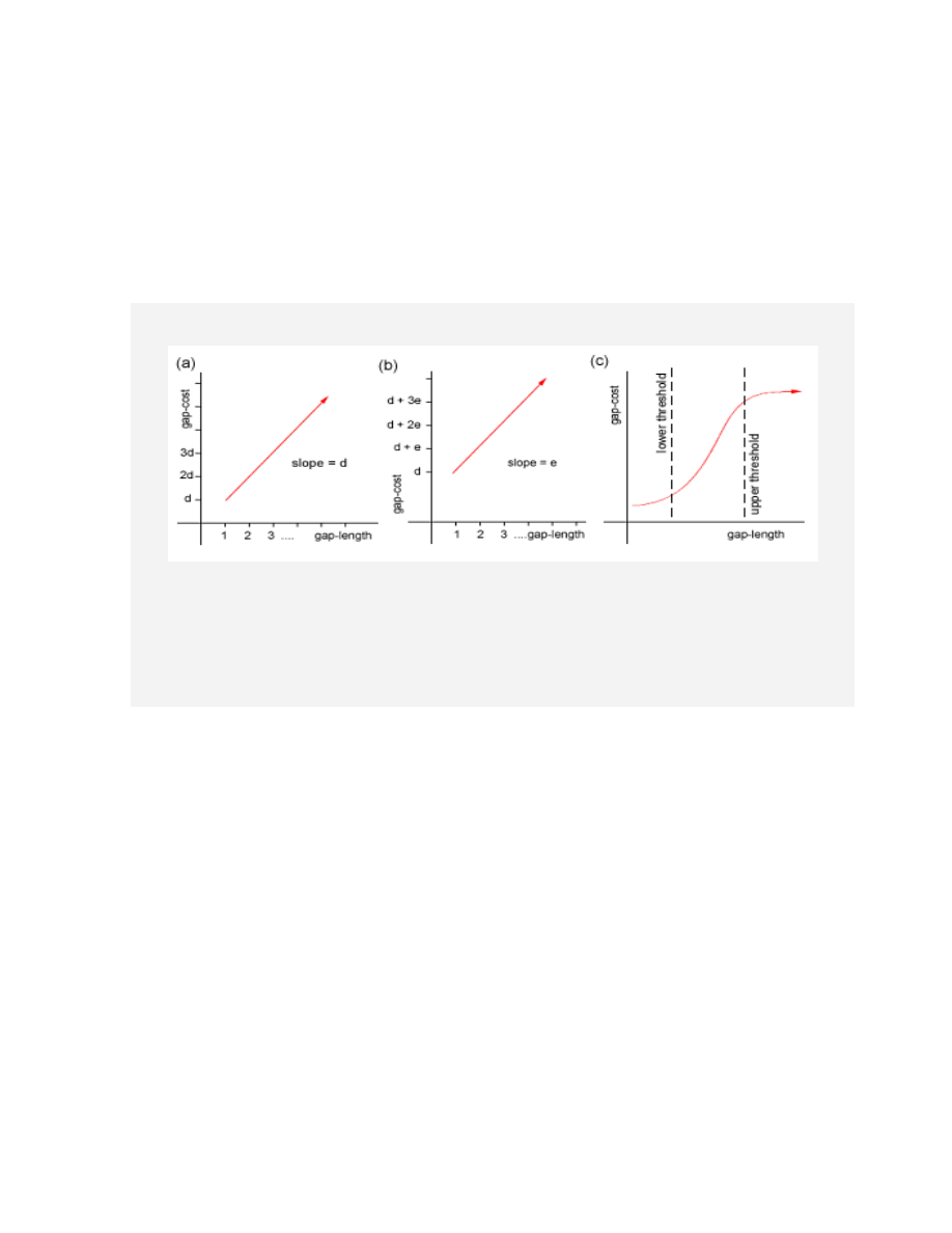
32

instructions. Also, a virus generator could insert ‘junk-code’ – which suggests when

aligning larger sequences there could be groups of entire subroutines or blocks which will

not align at all. This suggests that the ideal gap cost for aligning op-codes will look

something like the (c) in Figure 7.

Figure 7. Gap Penalty Graphs. (a) Linear Gap Penalty, (b) Affine Gap Penalty, (c)

Proposed Gap Penalty for op-code alignments

In the proposed gap penalty graph (c) of Figure 7, below the lower threshold and above

the upper threshold the gap costs do not increase much. The actual values of the gap

penalties will, similar to the scoring matrix, probably need to be guessed up front, then

refined as time goes on when more test results are available to produce higher quality

alignments. For initial research purposes, a simple affine gap penalty with values selected

by trial and error will be used. Future research can be done to determine if the gap

penalty function in (c) is more affective.

33

6.5

Pairwise Alignment Using Dynamic Programming

The next step to actually create an alignment will be to describe the algorithm which will

be used to produce alignments using the scoring mechanisms defined in the previous

section. Although there may be several different ways to produce a high scoring

alignment, the algorithm which will be used in this project will use a dynamic

programming approach.

The central idea behind this dynamic programming algorithm is to divide and conquer by

using information gathered from alignments created for smaller subsequences to

construct the optimal alignment for the entire sequence. The algorithm description below

is taken in part from [5] with some enhancements to generalize the gap scoring function

(denoted by g) – this algorithm is the mathematical basis behind the prototype developed

in this project.

Pairwise Alignment Algorithm Specification

Definitions

x = first sequence

y = second sequence

|a| = length of sequence a

a

i

= indicates the ith symbol of sequence a

a

i…j

= subsequence of a with indices i to j, where a

 a

1…|a|

s(a, b) = score assigned to substituting symbols a with b

g(n) = cost of adding one gap to a sequence with n-1 gaps

34

F and G = matrix of size |x|+1

 |y|+1 (indices will be 0 based)

F(i, j) = optimal score for aligning x

1…i

with y

1…j

G(i, j) = number of subsequent gaps used to generate F(i, j)

Recursive definition of F and G for i, j

 0

G(i, 0) = F(i, 0) = 0

G(0, j) = j

F(0, j) =





j

n

n

g

1

)

( (the cost of aligning j gaps)

1

)

1

,

(

)

,

(

3)

(case

if

1

)

,

1

(

)

,

(

2)

(case

if

0

)

,

(

1)

(case

if

3)

(case

)).

1

,

(

(

)

1

,

(

2)

(case

)),

,

1

(

(

)

,

1

(

1)

(case

),

,

(

)

1

,

1

(

max

)

,

(













































j

i

G

j

i

G

j

i

G

j

i

G

j

i

G

j

i

G

g

j

i

F

j

i

G

g

j

i

F

y

x

s

j

i

F

j

i

F

i

i

Pseudo code:

Initialize the first row in F and G : G(0, j) = j and F(0, j) =





j

n

n

g

1

)

(

For each row i, 1…|x|

Initialize F(i, 0) = 0 and G(i, 0) = 0

For each column j, 1…|y|

(i - 1, j - 1), (i - 1, j) and (i, j - 1) for F and G are all known

Calculate F(i, j) and G(i, j) using the recursive definition

35

6.5.1 Reconstructing the Alignment

In the above algorithm definition, the value in F(|x|, |y|) is the score for the optimal

alignment of the sequences x and y. In order to find the alignment which produced this

score, the implementation of this algorithm will need to keep trace-back pointers for each

cell in F. The trace back pointers can be set when calculating the index (i, j), depending

on the 3 cases defined in the recursive definition of F and G.

Case 1: (i, j)

 (i-1, j-1)

: indicates x

i

was aligned with y

j

(no gap)

Case 2: (i, j)

 (i-1, j)

: indicates a gap was inserted into x

Case 3: (i, j)

 (i, j-1)

: indicates a gap was inserted into y

Using these trace-back pointers, the decisions which lead to the final score F(|x|, |y|) can

be mapped back to F(0, 0) and the final alignment can then be reconstructed.

6.5.2 Algorithm Efficiency

In most cases, the algorithm to create an alignment is considered a one-time cost – which

means efficiency within the algorithm is not as important as the quality of the results.

However it is still important to analyze the efficiency, if only to be able to estimate the

kind of resources needed to generate alignments given the input sequences.

In the pseudo code there are 2 for loops where all the work is done to populate F and G,

where the inner loop requires a total of |x|∙|y| iterations. The reconstruction of the

alignment will require a maximum of |x|+|y| steps to follow the the trace-back pointers.

This means that the total time spent given 2 sequences of size n will be O(n

2

+ 2n) =

36

O(n

2

); and since the only space allocated is for G and F, the space complexity will be

O(2n

2

) = O(n

2

).

Although to use the dynamic programming algorithm, not much can be done about the

time complexity, the space complexity can be reduced from O(n

2

) to O(n) [5]. The

enhancement to improve the space complexity is detailed out in [5]; however, the space

complexity O(n

2

) will be acceptable for the purposes of this project.

7 Multiple Sequence Alignment

A pairwise alignment is a special case of a multiple alignment which involves only 2

sequences. When dealing with more than 2 sequences the problem of creating a multiple

alignment becomes much more complicated. In most cases, if the set of sequences align

well, more information can be retrieved from a multiple alignment because trends within

a larger set of data can be identified more clearly.

There are many different approaches to creating an MSA, in cases where the number of

sequences being aligned is small enough, an alignment can be created by hand, usually by

someone with an expert understanding of how the sequences are related, and also how

sequences can mutate over time to produce the alignment. Because the alignment was

created by hand, one would expect a very meaningful and high quality alignment. It is

obvious, though, that as the number of sequences grows the need for an automated way to

produce a high quality multiple alignment rises.

37

7.1

Progressive Alignment Algorithm

One of the simplest forms of automatically creating an MSA for an arbitrary set of

sequences is to use a progressive alignment algorithm. This kind of algorithm usually

starts off with an initial pairwise alignment and then builds on it by adding new

alignments with one by one until all sequences are included. The following is a

generalization of the algorithm:

Progressive Alignment Algorithm Specification

Definitions

M = set of aligned sequences

S = the input set of sequences

P(a, b) = the sequence a after aligning it with b

G(a, b) = the sequence a after adding any corresponding “new” gaps in b

Pseudo code:

Step 1:

Choose a, b

 S; remove a, b from S; add P(a, b), P(b, a) to M

Step 2:

Choose x

 M, y  S; then remove y from S

Step 3:

 z  M, update z = G( z, P( x , y ) )

Step 4:

Add P( y , x ) to M

Step 5:

if S is not empty go to step 2

In the above pseudo code, step 1 will initialize the MSA with a single alignment, and then

going forward all alignments will be created using one sequence already in the alignment

(denoted by x) and one sequence not in the alignment (denoted by y); the result of which

38

is added into the final alignment. In order for the existing sequences in the alignment to

match with the new alignment, any “new” gap inserted into x needs to also be applied to

all existing sequences in M (denoted by z). It is important to note that “new” here means

that it is likely that x already has gaps, due to the fact it came from M and has already

been aligned to one or more sequences. This process of matching gaps from one sequence

into another is denoted by the function G, which is demonstrated here with an example:

Assume:

x = ‘ABCDEFGHIJ’

y = ‘ABEXXFGXHI’

P( x , y ) = ‘ABCDE--FG-HIJ’

P ( y, x ) = ‘AB--EXXFGXHI-’

z = ‘0123456789’

Results of G:

G(z, P(x, y)) = ‘01234--56-789’

G(z, P(y, x)) = ‘01--23456789-’

In the algorithm, the function P is representative of standard pairwise alignment;

however, normally alignments are created for sequences which do not yet contain the

special character representing a gap. This may cause a problem in the alignment

algorithm since there was no defined way to substitute a gap for an existing symbol. In

order to fix this, the easiest solution is to add a new symbol to the sequence alphabet

which is considered “neutral” [5]. For example, one could declare the ‘+’ symbol as

neutral which will replace any gaps in step 4. In the Feng-Doolittle algorithm the neutral

39

symbol is given as an X [7]; however, in this application X already exists in the alphabet

and cannot be used. When scoring, the alignment will always assign a score of 0 for a

deletion or substitution of any neutral symbols. This addition also allows the easy

distinction between an “old” gap and a “new” gap (information needed in step 3) since

gaps that are “new” will be the gap symbol, and “old” gaps will be the neutral symbol.

In later sections this algorithm will be referred to as being composed of an initial

alignment step followed by a series of “iterations”; or more precisely for a set of n

alignments, there will be 1 initial alignment followed by n-2 iterations.

7.1.1 Choosing Alignments

Although the algorithm is fairly straightforward, the first and second steps require a

choice to be made leading to variations of this algorithm which will produce different

results. The variation stems from the fact that the choice of alignments and the order

which they are added can have an affect on the overall score and quality of that

alignment. A simple, but naïve, implementation would be to simply choose the

alignments at random; however, this would be less than ideal if one of the alignments

added had a low score.

Another more sophisticated approach, which was first introduced in the Feng-Doolittle

progressive alignment algorithm [7], would be to pre-calculate all the possible alignment

scores between pairs of sequences, and then select n-1 alignments which connect all

sequences and maximize the pairwise alignment scores.

Once the scores are calculated, one possible way to represent this data would be as an

undirected fully-connected graph in which the vertices represent the sequences and the

40

edges are assigned distance values equivalent to the alignment scores between the

sequences. When the data is represented this way, it is the problem to choose the

alignments (i.e. the edges in the graph) to maximize the score can be reduced to a

commonly known problem in graph theory of producing a minimum spanning tree. The

only difference is we are trying to maximize the cost of the spanning tree, which can

easily be fixed if we just multiply all scores by -1 and offset all scores to be positive.

In the Feng-Doolittle algorithm, this spanning tree is referred to as a guide tree which is

calculated using the clustering algorithm by Fitch & Margoliash [5]; however, the

algorithm chosen in this paper will be a variation of Prim’s algorithm [17]. After

calculating the minimum spanning tree, the alignment choices are simply the edges seen

in order when traversing through the entire tree starting from the alignment with the

highest score. An example of this selection process will be provided in the next section.

7.1.2 Example Multiple Alignment

In order to properly demonstrate the algorithm, an example MSA will be created using 10

op-code sequences taken from the NGVCK virus set. The sequences have been trimmed

down to a single subroutine from each of the viruses to simplify the example.

In Figure 8, a distance matrix is presented with all possible alignment scores among the

10 sequences, along with a representation of the spanning tree. Note that the scores in the

matrix for aligning a sequence with itself are not given because these scores will not

provide any useful information to the algorithm. One other thing to notice is that the

matrix is reflective – aligning a sequence i with sequence j is the same as aligning j with

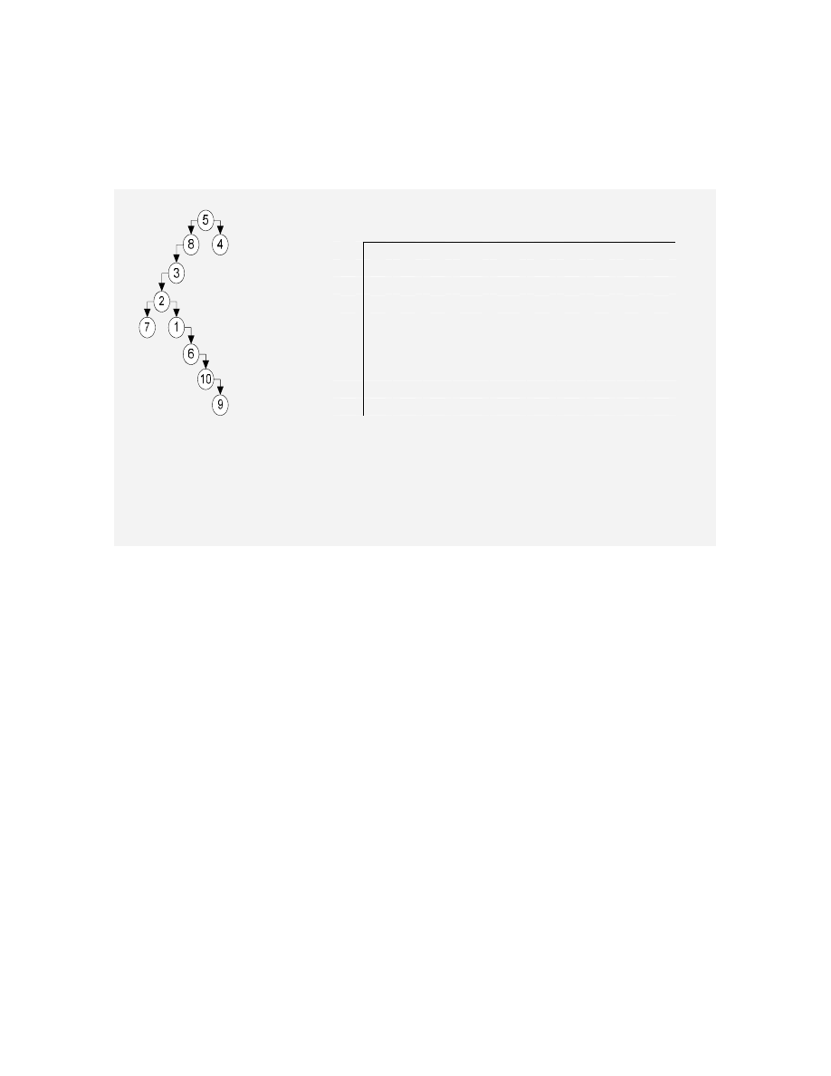
41

i. The alignment choices presented to construct the spanning tree were selected by the

prototype developed, which used a variation of Prim’s algorithm [17].

(a)

(b)

1

2

3

4

5

6

7

8

9

10

1

---

85

63

74

70

84

61

57

62

70

2

85

---

79

73

66

59

94

61

59

51

3

63

79

---

75

68

60

55

85

52

65

4

74

73

75

---

105

54

60

78

59

53

5

70

66

68

105

---

40

61

79

58

39

6

84

59

60

54

40

---

68

45

75

78

7

61

94

55

60

61

68

---

64

72

42

8

57

61

85

78

79

45

64

---

50

70

9

62

59

52

59

58

75

72

50

---

81

10

70

51

65

53

39

78

42

70

81

---

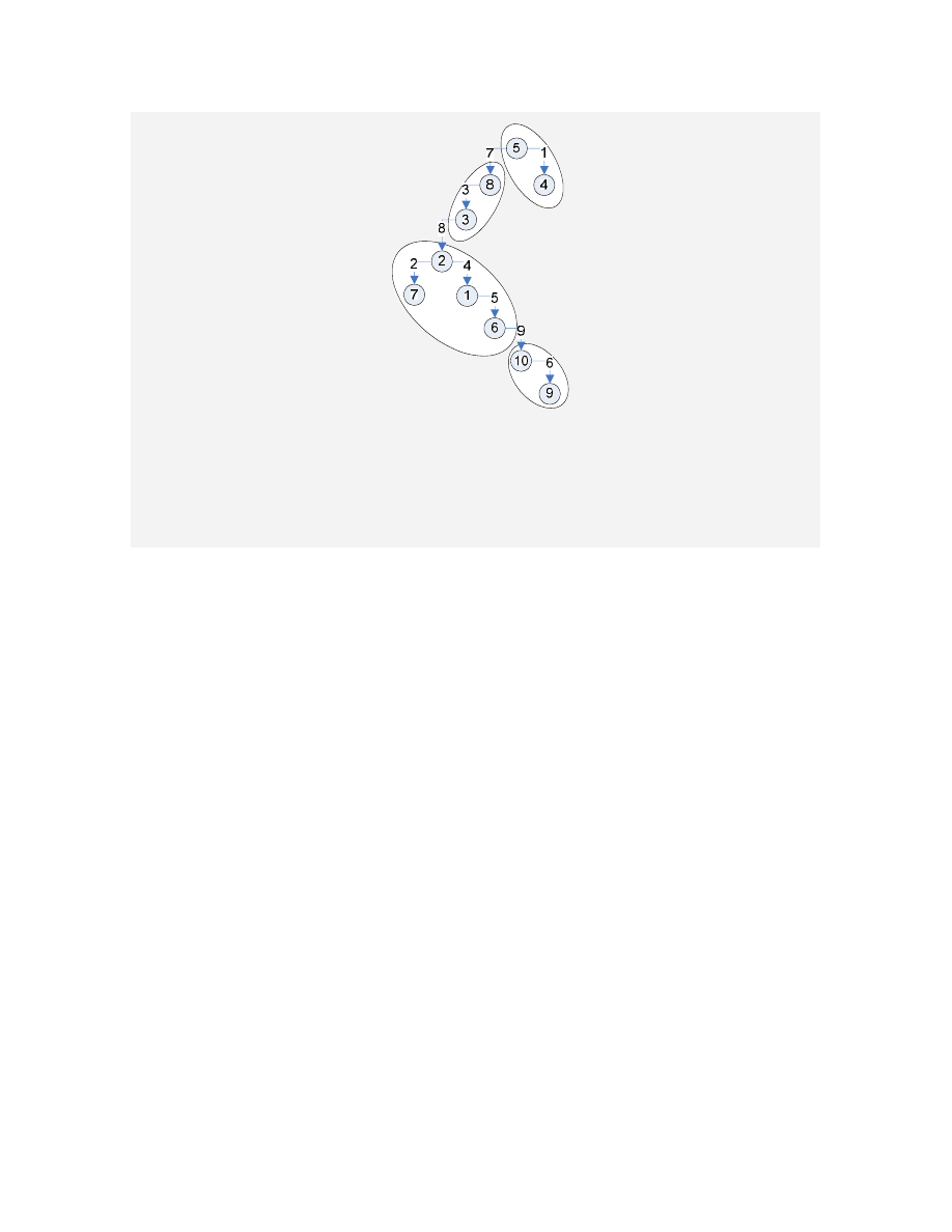
Figure 8.Minimum-Spanning Tree for adding Alignments, (a) The resulting tree,

(b) score matrix with the high score choices bolded and italicized

For the purposes of this example an alignment will be referred to as an ordered pair of

indices in which the first number represents the index of the sequence which already

exists in the MSA, and the second is the index of the sequence which is new to this

alignment (except for the first selected alignment in which both sequences are not

currently in the MSA and the ordering is arbitrary). Once the spanning tree is calculated,

the MSA is first initialized with the highest scoring alignment; in this case the alignment

(5, 4) is chosen. After the initial alignment, the following 8 alignments (corresponding to

the 8 iterations needed to align 10 sequences) are added in order: (5, 8), (8, 3), (3, 2), (2,

7), (2, 1), (1, 6), (6, 10), (10, 9).

In addition to this, Figure 9 provides a snapshot of the 3

rd

iteration which demonstrates an

iteration which a “new” gap is added (step 4 in the specification).

42

MSA Before New Alignment

5) CDABBAFCDB1AAEAA+CEDA+EQ+CDABABABALF4LBBAFBSBAAAAA
4) 2AABBAFCDABA+EAABCEDCDEQFCDABA+APALF4+BBA++SBAAAAA

8) ++AABA+CDB+AAEAA+CEDCDEQ+CDABPBA+ABF4+BBAFBSBMAAAA
3) A+ABBAFCDABA+EAA+CEDCDEQA++ABFBAN++F4+BBAFBTYBAAAA

New Alignment

2) A-ABNBAFCD-BAAEAABCEDA-EQ-CDABAB--BAF4NBBM-BTYBAAAA
3) A+AB-BAFCDABA+EAA+CEDCDEQA++ABFBAN++F4+BBAFBTYBAAAA

^ (gap introduced)

MSA After New Alignment

5) CDAB+BAFCDB1AAEAA+CEDA+EQ+CDABABABALF4LBBAFBSBAAAAA

4) 2AAB+BAFCDABA+EAABCEDCDEQFCDABA+APALF4+BBA++SBAAAAA
8) ++AA+BA+CDB+AAEAA+CEDCDEQ+CDABPBA+ABF4+BBAFBSBMAAAA

3) A+AB+BAFCDABA+EAA+CEDCDEQA++ABFBAN++F4+BBAFBTYBAAAA
2) A+ABNBAFCD+BAAEAABCEDA+EQ+CDABAB++BAF4NBBM+BTYBAAAA

^ (gap matched)

Final alignment

1) A-AB-BAFCD-B-AAEA0ACEDA-EQ---A-ABCDBALF4-BBASB---AAAAFB

2) A-ABNBAFCD-B-AAEAABCEDA-EQ-CDABAB--BA-F4NBBM-BTYBAAAA--
3) A-AB-BAFCDAB-A-EAA-CEDCDEQA--ABFBAN---F4-BBAFBTYBAAAA--

4) 2AAB-BAFCDAB-A-EAABCEDCDEQFCDABA-APAL-F4-BBA--SBAAAAA--
5) CDAB-BAFCDB1-AAEAA-CEDA-EQ-CDABABABAL-F4LBBAFBSBAAAAA--

6) CDABAAA----B-A-EA-ACEDCDEQ---A-ABCD-A-F4-BBASB---AAAAFB
7) CDAB--A-CDAB-A-EAA-CEDA-EQ-CDABCDCDAA-F4MBB--ATYBAAAA--

8) --AA-BA-CDB--AAEAA-CEDCDEQ-CDABPBA-AB-F4-BBAFBSBMAAAA--
9) CDAB--RBAFABPAAEA-ACEDCDEQAABCDAFAL---F4NBBASB---AAAAMB

10) A-ABAA-----B-AAEA-ACEDCDEQAABAFA------F4BNBASB---AAAAFB

Figure 9. Snapshot of 3

rd

iteration in the progressive MSA algorithm. In this

snapshot the (3,2) alignment is added to the MSA, and a “new” gap appears in 3

43

7.1.3 Ordering Alignment Insertions

When creating a spanning tree which maximizes the alignment scores, the order that the

alignments are added to the cumulative MSA will affect the final result. This is due to the

fact that alignments are created on already gapped sequences which will affect the

placement of aligned subsequences in the optimum pairwise alignment. In order to

determine how much affect that different sequences of alignment insertions will have on

a multiple alignment, the progressive algorithm discussed earlier will be modified to

allow edges in the graph (or pairwise alignments) to be added in any order as long as the

edges follow the minimum spanning tree. After the distance matrix is known, the

algorithm will consist of two parts: calculating the minimum spanning tree, then inserting

progressively combining sequences in the spanning tree to form the multiple alignment.

Because edges can be added to the MSA in any order, multiple small sub-trees will be

formed representing smaller sub-alignments. When an edge is added to combine two sub-

trees the two smaller MSAs can be combined by matching the newly inserted gaps in

each of the two sub-trees. This will continue until the entire spanning tree is covered and

a multiple alignment containing all sequences has been created.

To test the how much affect the ordering has on the multiple alignments, several insertion

sequences were tried:

1) Following the minimum spanning tree, start with the highest scoring pairwise

alignment then add edges to a single cumulative multiple alignment until the

entire tree is covered (this is the ordering suggested in Section 7.1.2)

2) The exact opposite of 1)

44

3) Add the edges in the graph from highest scoring to lowest scoring

4) The exact opposite of 3)

These insertion sequences were then used to create four multiple alignments for a group

of 20 viruses from the Next Generation Virus Creation Kit (NGVCK), which will be

discussed in the case study in Section 7.3, and the results showed that there were

variations within the four resulting MSAs.

In the example provided in Section 7.1.2 the following edges will be selected for the 4

insertion sequences:

Edge 1

2

3

4

5

6

7

8

9

1) Edges: (5, 4), (5, 8), (8, 3), (3, 2), (2, 7), (2, 1), (1, 6), (6, 10),(10, 9)

Scores: 105, 79,

85,

79,

94,

85,

84,

78,

81

2) Edges: (10, 9), (6, 10),(1, 6), (2, 1), (2, 7), (3, 2), (8, 3), (5, 8), (4, 5)

Scores: 81,

78,

84,

85,

94,

79,

85,

79,

105

3) Edges: (5, 4), (7, 2), (3, 8), (2, 1), (1, 6), (10, 9), (5, 8), (3, 2), (6, 10)

Scores:105,

94,

85,

85,

84,

81,

79,

79,

78

4) Edges: (6, 10), (3, 2), (5, 8), (10, 9),(1, 6) (2, 1), (3, 8), (7, 2), (5, 4)

Scores:78,

79,

79,

81,

84,

85,

85,

94,

105

Figure 10. Example ordering for each of the four chosen insertion sequences

45

Figure 11. Sub-trees given in a spanning forest created after inserting the 6

th

edge in the

3

rd

insertion sequence

In Figure 10 above, a snapshot of a spanning forest which is created after the 6

th

edge is

added in the 3

rd

insertion sequence (ordering edges from highest score to lowest). Once

the 7

th

edge is added attaching sequence 5 and sequence 8, the two smaller sub-

alignments of size two each are combined (sub-trees {5,4} and {8, 3}) to create a larger

sub-alignment of size four (sub-tree {5,4,8,3}). Subsequently adding edges 8 and 9 will

cover the entire spanning tree.

The percentage of gaps in each of the four alignments was about the same, with a

difference of less than 1%. The percent of gaps will be used as a crude measurement of

alignment quality (discussed further in Section 7.2). Interestingly, the MSAs created for

the 1

st

and 3

rd

insertion sequences were similar in appearance after subjective inspection;

conversely the 2

nd

and 4

th

insertion sequences were also similar. This may require some

additional future analysis to determine exactly how similar or dissimilar the MSAs

created using different insertion sequences by using some objective similarity index;

46

however the quality of the alignments created did not vary significantly. The resulting

MSAs were then used to train the profile HMM researched in [2] and the resulting scores

where only insignificantly affected, suggesting that the order of sequence insertions does

not greatly affect the stability of the resulting profile HMMs.

7.1.4 Algorithm Efficiency

The iterative algorithm uses the pairwise alignment as a subroutine, which has both space

and time complexity of O(n

2

) for a sequence of size n. In this case, there are some

variations of the time/space complexities due to the input data.

Best-case scenario:

The sequences are highly related and the final multiple alignment will contain

aligned sequences which are no more than cn in length, where c is a constant and

n is the maximum length of the input sequences.

Worst-case scenario:

The sequences are not related at all, none of the symbols get aligned and the

maximum amount of gaps are inserted into each sequence. In this case if m

sequences are given, and the length each sequence is n, then the number of gaps

in each sequence in the resulting alignment will be n∙(m-1).

Time Complexity:

Input: Given m sequences each of size n

T

1

= Time to pre-calculate the matrix of all scores

= The time it requires m∙(m-1)/2 alignments = O(m

2

)∙O(n

2

) = O(m

2

n

2

)

T

2

= Time to create the spanning tree using Prim’s algorithm = O(m

2

)

47

T

3

= Time to for initial alignment O(n

2

)

T

4

= (best-case) Time for each addition alignment = (m-1) ∙ O(n

2

) = O(mn

2

)

T

4

= (worst-case) Time for each additional alignment =

)

(

)

(

2

2

2

2

n

m

O

in

O

m

i







Total Time = T

1

+T

2

+T

3

+T

4

= O(m

2

n

2

) (in either the best or the worst case).

Space Complexity:

This will be defined by the amount of space required calculate the pairwise

alignment for the longest chosen sequence

(best-case) : max size sequence = O(n), space complexity = O(n

2

)

(worst-case): max size alignment = O(mn), space complexity = O(m

2

n

2

)

Thus, the space complexity can be anywhere between O(n

2

) and O(m

2

n

2

)

depending on how well the sequences align in the MSA

Similar to the algorithm to create pairwise alignments, any algorithm to create a multiple

alignment will value the quality of the results over efficiency; however, it is important to

note that the amount of time and space required to execute the program will increase

dramatically if the sequences do not align well – so the better these sequences align, the

more efficient the overall algorithm will be.

7.2

Determining Alignment Quality

There are many possible multiple alignments which can be created, and it is important to

clearly distinguish the problem of creating an alignment and the problem of determining

how well the sequences were aligned. There are many different measures of quality for

multiple alignments, some more complicated than others.

48

One common way to score a multiple alignment which is a natural extension of the

scoring mechanism defined for simple pairwise alignment uses the same substitution

matrix used before in scoring pairwise alignments but this time it is used to calculate a

cumulative score for each column in the alignment using a simple mathematical formula.

The full definition of this scoring function can be found in [5].

Although the cumulative substitution score is a useful measure of quality, in this project I

have defined a much simpler means of calculating the relative quality of an alignment:

the ratio of symbols to gaps. This ratio will be referred to by the term “conservation

percentage”, in which a low percentage means that the sequences were poorly aligned

resulting in too many gaps. When using the alignment to train a profile HMM, the

amount of conservation within the alignment will greatly affect the quality of that profile

HMM making the conservation percentage more valuable a metric than the cumulative

substitution scores.

7.3

Case Study: NGVCK Virus Alignment

The Next Generation Virus Creation Kit (NGVCK) is a virus generator which can

automatically generate variations of a virus. The NGVCK generator has an advanced

assembly source-morphing engine which includes random function ordering, junk code

insertion, and user-defined encryption methods [12]. This means that all variants of the

viruses generated by NGVCK will all have the same functionality, but they will all look

very different from one another. A similarity score was introduced in [18] which shows

that the viruses showed significantly more variation than many other commonly known

virus generators. From this definition, the NGVCK virus generator can be considered a

49

metamorphic virus, and because of its significant variation it will be considered the

“difficult” case which should sufficiently test the theory that a meaningful alignment can

be created for a highly metamorphic virus. Tests on the viruses generated by NGVCK

will provide valuable information since the virus demonstrates all 4 of the mutational

processes: insertions, deletions, substitutions, and permutations. In particular, the results

of analysis will also show how well the preprocessing algorithm using subroutine

matching increases the quality of the produced pairwise and multiple alignments.

In [18], a particular set of 200 viruses generated by NGVCK was analyzed in great detail;

for consistency this same set of 200 viruses (courtesy of Dr. Mark Stamp) will be tested

here as well. The following properties were used when creating the alignments:

Alphabet = Defined in Figure 1

Scoring Substitution Matrix = Defined in Figure 6

Gap Scoring Mechanism = Affine Gap with gap-open cost of 10 and extension cost 1

Two copies of the 200 viruses were created for testing purposes:

 The unmodified virus op-code sequences

 Modified op-code sequences in which all sequences were preprocessed to

maximize the alignment scores by attempting to reverse any permutations done by

the NGVCK generator.

The first test on each of the sets of viruses was to take one group of 40 viruses and create

a simple pairwise alignment on each possible pair of sequences within the group, or a

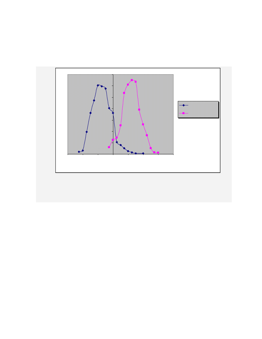
50

total of

780

2

40 













alignments. The distribution of the scores for the alignments created

is represented in Figure 10.

0

20

40

60

80

100

120

140

-6

-4

-2

0

2

4

6

8

Score

#

o

f

A

li

g

n

m

e

n

ts

Raw Sequences

Preprocessed

Figure 12. Score Distributions for both NGVCK test sets with sample size 780

In this graph, clearly the preprocessed viruses generate a much better score on average.

The next step is to analyze the multiple alignments created for NGVCK using the

progressive alignment algorithm and the pairwise alignments created in the first step.

Multiple Alignment Results for Raw sequences: The results showed that the amount of

gaps being inserted into the raw sequences was staggering. In Figure 11, the conservation

percentages for raw sequences are extremely low. This result was not surprising: as

expected the permutation engine has adversely affected the alignments.

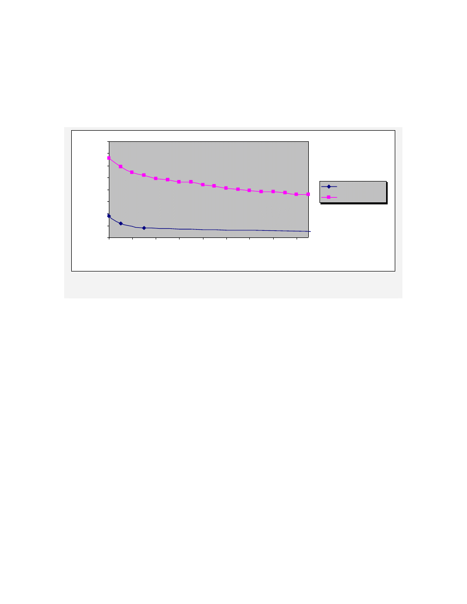
51

Results for Preprocessed Sequences: The results showed promise, the conservation

percentage of the preprocessed sequences is almost 70% for a group size of 10, and

slowly drops off as the number of sequences grows.

0%

10%

20%

30%

40%

50%

60%

70%

80%

10

30

50

70

90

110

130

150

170

Group Size

C

o

n

s

e

rv

a

ti

o

n

%

Raw Sequences

Preprocessed

Figure 13. Conservation percentage based on group size for NGVCK

In Figures 12 and 13, a graphical representation of an MSA is given in which a symbol is

represented as a black pixel and a gap is represented as white space. These images were

created by a simple Java application created specifically for the purpose of generating

these kinds of images.

52

Figure 14. Graphical representation of groups of 20 preprocessed NGVCK

viruses. The width of the image has been reduced by half

Figure 15. Graphical representation of groups of 20 raw NGVCK viruses. Width

of the image has been reduced to 1/10

th

the original size

53

7.4

Case Study: VCL32 and PS-MPC Virus Alignments

Two other viruses which were studied in [18] are the Virus Creation Lab for Win32

(VCL32), and Phalcon/Skism Mass-Produced Code Generator (PS-MPC). Unlike

NGVCK, these virus generators do not use function permutation when creating variations

of the virus.

The test sets were made up of 10 viruses from VCL32 and 30 viruses from PS-MPC. The

distributions of the pairwise alignments for the op-code sequences are shown in Figure

12. Because there are only 10 variations of the VCL32 virus, the number of alignments in

the graph was adjusted for a sample size of













2

10 = 45 alignments.

From the graphs in figures 14 and 15 the following can be concluded:

 The VCL32 virus scored higher with pairwise alignments and had a higher

conservation percentages than the other virus test sets

 the PS-MPC viruses mostly positive pairwise alignment scores but had a high

amount deviation in the distribution

 The multiple alignments created for PS-MPC viruses and the preprocessed

NGVCK viruses had about the same amount of conservation for group sizes of 3

to 30

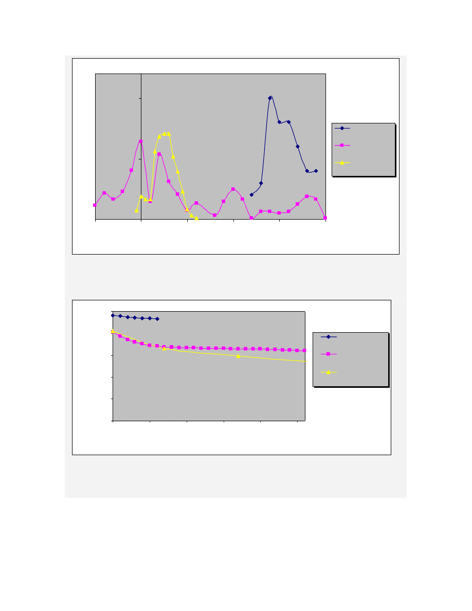
54

0

5

10

-5

0

5

10

15

20

Score

#

o

f

A

li

g

n

m

e

n

ts

VCL32

PS-MPC

NGVCK
(Preprocessed)

Figure 16. Score distributions for VCL32, PS-MPC, and NGVCK (Preprocessed)
adjusted for a sample size of 45 alignments

0%

20%

40%

60%

80%

100%

3

8

13

18

23

28

Group Size

C

o

n

s

e

rv

a

ti

o

n

%

VCL32

PS-MPC

NGVCK
(Preprocessed)

Figure 17. Conservation Percentage of VCL32, PS-MPC, and NGVCK
(Preprocessed) virus op-code sequence generated multiple alignments.

A graphical representation of the MSA’s for PS-MPC and VCL32 are given in Figure 16.

For display purposes, the height of the images were tripled in size and the width of the

55

VCL32 image was reduced by 1/8

th

. These images were produced by the same java

application used in the figures 12 and 13.

(a) MSA for two groups of 15 PS-MPC viruses

(b) MSA for 10 VCL32 viruses

Figure 18. Graphical representations of MSA’s created for PS-MPC and VCL32

8 Preliminary Profile HMM Results

The multiple alignments created in the case studies presented in this paper were given to

another student, Srilatha Attaluri, researching the profile HMM piece of the new virus

detection approach. The results of the tests can be measured by the following criteria:

 False-positive rate: The percent of non-virus files that were incorrectly identified

as a virus

 False-negative rate: The percent of virus files that were correctly identified as a

non-virus

56

The initial results indicate that for the PS-MPC and VCL32 viruses the generated profile

HMMs resulted in a 0% false-positive rate and a 0% false-negative rate. The NGVCK

viruses displayed varying results depending on the threshold value selected [2].

 16.95% false-positive rate, 0% false-negative rate when using the minimum

value as the threshold

 8.7% false-positive rate, 0.5% false-negative rate when using the second

minimum value as the threshold

 6.8% false-positive rate, 1% false-negative rate when using the third minimum

value as the threshold. [2]

9 Future Research Needed

9.1

Scoring Refinement

It is important to note that the values in the scoring matrix defined for this project (Figure

6) as well as those defined in the gap scoring mechanism used were only an initial

attempt or a guess for the values. This means that resulting alignment scores should only

be used for comparing two alignments to determine if one alignment is “better” than

another – the actual value will not be representative of any quantifiable properties of the

sequences for which the alignment was created.

That being said, there is still work to refine the actual values in the scoring matrix; the

refinement could take into account expert knowledge of the actual op-codes which the

symbols represent and determine for each possible pair of op-codes how likely is it that a

metamorphic virus will decide to substitute the op-codes for one another. This kind of

analysis may require some extensive research to produce statistics about substitutions for

57

various op-codes. It may even be possible to refine the matrix even further depending on

the actual virus which the scoring matrix will be used against, which could get even more

in depth assuming that the virus is known and this specific information about the virus

can be extracted.

Armed with this additional information, the substitution matrix could be enhanced and

the alignments generated using this new matrix would likely improve as well; however,

this kind of research is only needed to refine the scores, since it was not necessarily

important for this project to generate perfect multiple alignments in order to prove the

concept that a high quality alignment can be generated.

One possible strategy to refine the scores without having a complete statistical work-up

of possible substitutions would be to analyze each instruction and define groups of op-

codes which have similar functions. For example all op-codes which define a branch

could be one group, and op-codes which perform a mathematical function could be

another group. Then one could add additional criteria used to generate the substitution

matrix presented in Figure 6 so that any substitution within an op-code group would give

a positive score, and any substitution outside of the group would give a negative score.

This analysis is left open for future research.

9.2

Affects of Preprocessing on a Profile HMM

It was clear from the results of the NGVCK test set described in Section 7.3 that the

alignments generated for the raw op-code sequences of highly metamorphic viruses

would likely be of such a low quality that it would not produce much of a result when it

is used to train a profile HMM to detect the virus. To improve the alignments, a

58

preprocessing step was introduced which would permute the file in such a way that the

scores would be maximized; however, the affects of doing so is not clearly known.

It is likely that in order for the profile HMM to correctly score an arbitrary input

sequence, the same preprocessing step must be performed on the input sequence.

Assuming that the input sequence to the profile HMM was part of the same virus family,

the preprocessing step would easily permute the virus in the way the viruses used to

create the MSA were permuted; however, the input sequence is arbitrary and is not

necessarily the same virus. Ideally since the preprocessing step would only maximize the

scores of a possible alignment by permuting the subroutines, the maximum score of a

preprocessed non-virus would still be low and thus the results of the profile HMM will

still recognize it as a non-virus, but this concept still must be explored.

10 Conclusion

There is still more research to be done to explore the results of a profile HMM to fully

conclude if the new virus detection approach will successfully detect metamorphic

viruses. The results from the case studies presented in this paper show that creating

multiple alignments which can be used to train the profile HMM is feasible assuming the

input sequences are not permuted. This assumption can be made either because the virus

does not have the feature to permute its subroutines or because the input sequences were

preprocessed to remove the permutations. There is still room for improvement left open

for future research of the algorithms presented in this paper which could possibly

improve the accuracy of the profile HMM. Although the preliminary results show that the

profile HMM is successful in detecting some kinds of viruses, more research is needed to

59

expand on the findings to determine if the profile HMM can be used to detect more

advanced metamorphic viruses.

11 References

[1]

Accelrys Inc., Profile Hidden Markov Model Analysis, 2001

http://www.liv.ac.uk/e-science/sun/apps/genetics/

gcghelp/hmmanalysis.html

[2]

S. Attaluri, Detecting Metamorphic Viruses using Profile Hidden Markov Models,

2007, masters thesis, Department of Computer Science, San José State University

[3]

D. Bilar, Statistical Structures: Fingerprinting Malware for Classification and

Analysis, Proceedings of the Black Hat Convention, Las Vegas 2006,

http://www.blackhat.com/presentations/bh-usa-06/BH-US-

06-Bilar.pdf

[4]

datarescue.com, Executive Summary: IDA Pro – at the cornerstone of IT security,

http://www.datarescue.com/idabase/ida-executive.pdf

[5]

R. Durbin et al, 1998, Biological Sequence Analysis: Probabilistic Models of

Proteins and Nucleic Acids, pp 12-45, 135-160

[6]

extremetech.com, Antivirus Research and Detection Techniques,

http://www.extremetech.com/article2/0,1697,1150886,00.

asp

[7]

Feng, D.-F and Doolittle, R. F. 1987. Progressive sequence alignment as a

prerequisite to correct phylogenetic trees. Journal of Molecular Biology and

Evolution 13:93-104.

[8]

R. G. Fiñones, 2006, Solving the Metamorphic Puzzle,

http://www.virusbtn.com/virusbulletin/archive/2006/03/

vb200603-metamorphics

[9]

goof.com, Pentium® Optimization Cross-Reference by Instruction,

http://www.goof.com/pcg/doc/pentium-optxref.html

60

[10]

D. Harley, A. Lee, Heuristic Analysis – Detecting Unknown Viruses, 2007,

http://www.eset.com/download/whitepapers/

ESET_Heuristic-Analysis_Feb2007.pdf

[12]

P. Ször, The Art of Computer Virus Research and Defense, 2005, Addison-

Wesley

[13]

P. Ször, P. Ferrie, Hunting for Metamorphic, Proceedings of Virus Bulletin

Conference 2001, http://www.peterszor.com/metamorp.pdf

[14]

F. Veldman, Heuristic Anti-Virus Technology, http://vx.netlux.org/

lib/static/vdat/epheurs1.htm

[15]

VX Heavens, vx.netlux.org/

[16]

www.wikipedia.org, Hidden Markov Model, http://en.wikipedia.org/

wiki/Hidden_Markov_Model

[17]

www.wikipedia.org, Prim’s Algorithm, http://en.wikipedia.org/

wiki/Prim%27s_algorithm

[18]

W. Wong, Hunting for Metamorphic Engines, http://www.cs.sjsu.edu/

faculty/stamp/papers/Wing.pdf