Geometric Algebra and Computer Vision

The Auto-calibration Problem

Chris Doran

Department of Physics

Madingley Road, Cambridge

[e-mail]

www.mrao.cam.ac.uk/

clifford/

SUMMARY

1.

Rotors, bivectors and rotations.

Ways of representing

rotations and the group manifold.

2.

Extrapolating rotors and rotor calculus.

The linear space

associated with rotors, extrapolating and averaging

rotations.

3.

The known range data problem.

Least squares, its

Bayesian origin and solution for 2 and

cameras.

4.

Unknown range data problem.

Bayesian analysis again

and its geometric solution. 2 camera data and the

-camera problem.

1

G

EOMETRIC

A

LGEBRA IN

3-

D

1 scalar

3 vectors

3 bivectors

1 trivector

NB

for the pseudoscalar. Geometric product has

Æ

Dot and wedge symbols have usual meaning

A

rotor

is a normalised element of the even subalgebra,

The tilde is the

reverse

operation. Rotors generate rotations

via

¼

We can also write

¾

R generates a rotation of

in a positive (right handed)

sense in the

plane. In 3-d we can also write

¾

where

is the unit vector representing the axis.

2

T

HE

G

ROUP

M

ANIFOLD

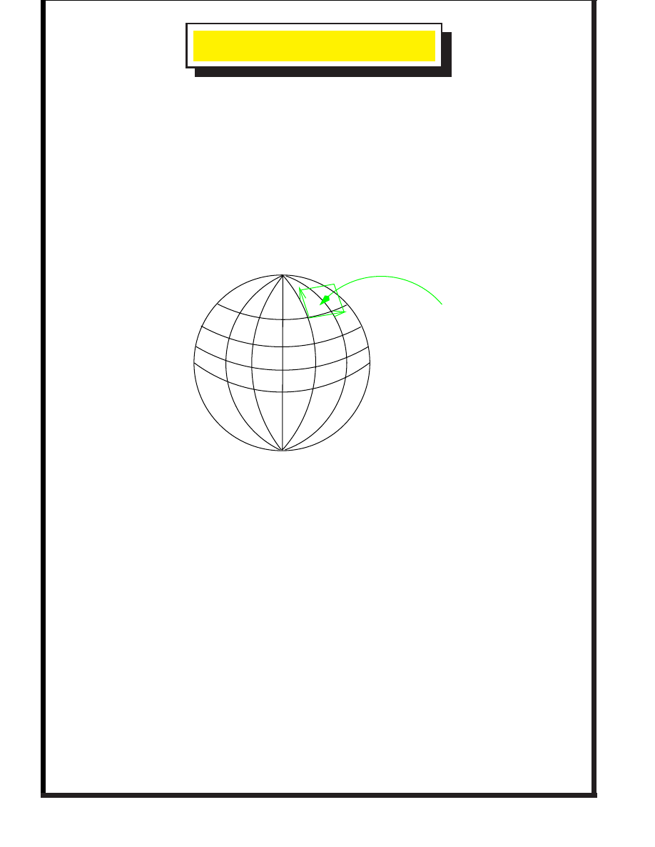
Rotors are elements of a 4-d space, normalised to 1. They lie

on a

3-sphere

. This is the

group manifold

. Any paths between

rotors must lie on this manifold.

At any point on the manifold, the

tangent space

is

3-dimensional. Just like the 2-sphere in 3-d:

Tangent plane

Rotors require 3 parameters, eg. Euler angles

½

¾

¾

¾

¿

¾

½

¾

¾

But often more convenient to use the set of bivector

generators

with

Small Complication:

The rotors

and

generate the

same

rotation. The

rotation

group manifold is more

complicated — it is a

projective 3-sphere

with

and

identified. Usually easier to work with rotors.

3

E

XTRAPOLATING

B

ETWEEN

R

OTATIONS

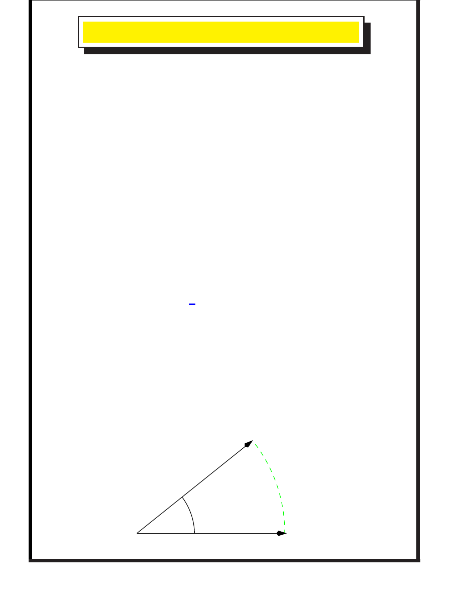
Given two estimates of a rotation,

and

, how do we find

the

mid-point

? With rotors this is

remarkably easy

! Make sure

they have smallest 4-d angle on 3-sphere. Path between them

is

so find

from

This path is

invariant

. If both endpoints are transformed, the

path transforms in the same way. The midpoint is

¾

This is

general

— works for any Lie group. For rotations in 3-d

can do even better.

and

can be viewed as two unit

vectors in 4-d. The above construction gives the path in the

plane specified by these vectors

4

The rotor path can therefore be written as (simple trig’)

and the midpoint rotor is simply

Gives a very simple prescription for finding the midpoint:

Add the rotors and normalise the result

Extremely simple! Compare with the equivalent matrix —

quadratic in

, so the expression is a mess.

These formulae are very useful in

dynamics

.

Averaging Rotations

Suppose now that we had a number of estimates for a rotation

and wanted to take the average. Again the answer is simple —

add up all of the rotors and normalise

(taking care to make

sure they are all in the ‘closest’ configuration). Useful in

computer vision

.

Lesson

Can simplify problems with rotations by relaxing the

normalisation criteria for rotors and working in the 4-d

linear

space. This provides us with one further additional tool:

5

R

OTOR

C

ALCULUS

Can view a function of a rotation as taking values over the

group manifold

. Calculus in these cases is possible, but a bit

messy. (Often resort to Euler angles.)

Now have a more elegant and simpler alternative: relax the

normalisation constraint and replace

by

— a

general

element of the even subalgebra. Start with simple result

where

contains only even-grade terms. Trick now is to write

 

Typical application is on scalar

 

where

projects onto scalar part. Now have

 

 

 

where overdot denotes scope.

6

Need a formula for the inverse term. Use

 

 

 

 

 

 

 

Can now complete derivation

 

 

 

 

Convenient to premultiply by

 

 

 

Note the

geometric product

. The result is a bivector — a

3-parameter space, as expected.

This simple derivation turns out to be very useful in a range of

applications.

7

C

OMPUTER

V

ISION

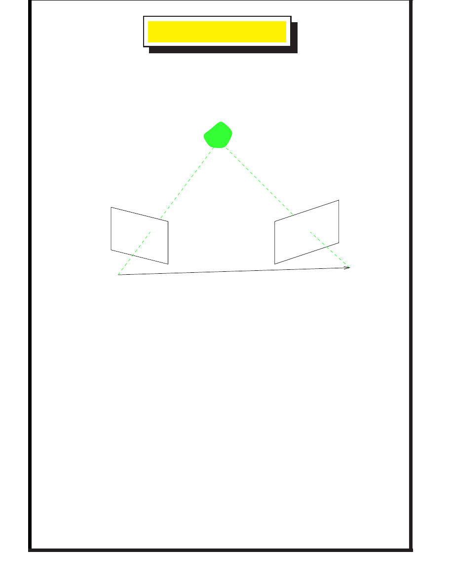
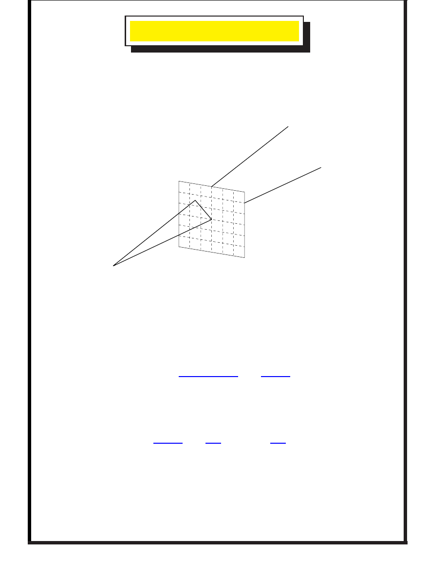
Basic problem of interest is the

auto-calibration problem

.

Suppose we have different camera views of the same scene.

Camera 1

Camera 2

Object

Given point matches (+ noise) can we figure out the relative

translation and rotation between the cameras (to calibrate).

Then use the calibrated cameras to reconstruct a 3-d scene.

Applications

1.

Gait analysis

— running etc.

2.

Motion analysis

— sports analysis and RSI in musicians

3.

Reaching and Neurogeometry

.

4.

3-d Reconstruction

eg. using a single moving camera

attached to a robot arm.

Two distinct problems to study.

8

K

NOWN

R

ANGE

D

ATA

Suppose we know the full 3-d positions of each point match

(not very likely in practice). Have coordinates

and

relative to first and second camera. With

the first camera

frame, define

¼

and have

Should have

¼

Want best fit

and

with various point matches. Minimise

least squares error

¼

There is a

Bayesian derivation

of this result. Start with

Gaussian distribution for the coordinates

(bar for ‘true’ position).

Marginalise

over actual positions to get

likelihood function in terms of data,

and

. Always useful to

see how expressions arise from a simple probabilistic

argument.

9

Solution

Differentiating

wrt

and

is straightforward

¼

so best fit,

, given by

¼

ie difference in centroids. For

derivative write

¼

¼

so just need

¼

 

¼

Substitute solution for

, get simply

where

¼

Easily solved with an

SVD

of

. Computationally

very

efficient

. A useful check on any reconstruction.

10

E

XTENSION TO

CAMERAS

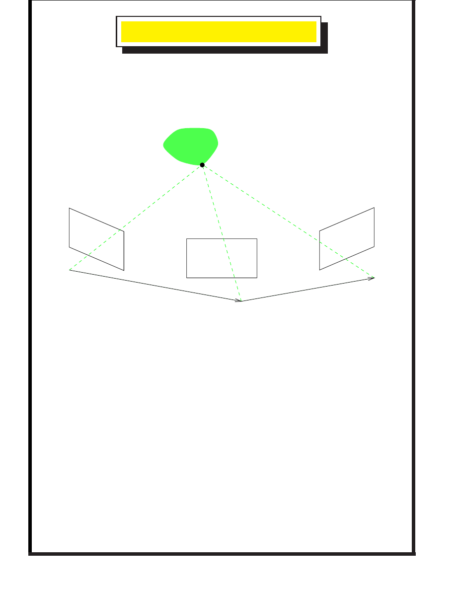
Get the general idea by considering 3 cameras. Express

everything in a

global

frame.

Camera 1

Camera 2

Camera 3

¼

¼

¼

Object

We could minimise

but this is not symmetric. Instead consider each pair in turn

with a

separate rotor

for each pair.

The rotors and translations should be consistent.

11

Impose

constraints

Can proceed as above for the translations. Find that

,

and

are still difference of centroids. The constraint is

automatically satisfied.

To find centroids we still need the rotors. Enforce rotor

constraint with a

Lagrange Multiplier

of form

must be a

multivector

Lagrange multiplier to ensure

consistency (Because normalisation is relaxed). Now take

, so final expression to minimise is

 

 

 

Get three equations, as preceding, each of form

½¾

12

For right-hand side use

so get same bivector for each of the three equations.

Introducing three tensor, one for each pair, get

symmetric

set

of equations

Want to find rotors to minimise mutual antisymmetric

contribution, subject to constraint

. Slightly

more complicated but not hard to solve numerically,

particularly as the individual pairwise minimisers are a good

starting point.

13

U

NKNOWN

R

ANGE

D

ATA

Usually we do not know the range data — instead we just

know the projective vectors on the camera plane

Image Plane

!

"

"

and choose scale with

,

 

,

"

Represent line

"

in 2-d with the

bivector

(taking

). Components

are

homogeneous coordinates

— independent of scale. Typically

these are measured.

14

Two main sources of

noise

:

1.

Pixelisation Noise

due to finite resolution.

2.

Random Noise

due to camera motion, etc. Assume to be

Gaussian.

Can get a likelihood function by marginalising over the

unknown range data. Do this with integrals of the type

#$

#$

¼

$

%

$

¼

%

¼

which gives a likelihood function going with

%

%

¼

%

%

¼

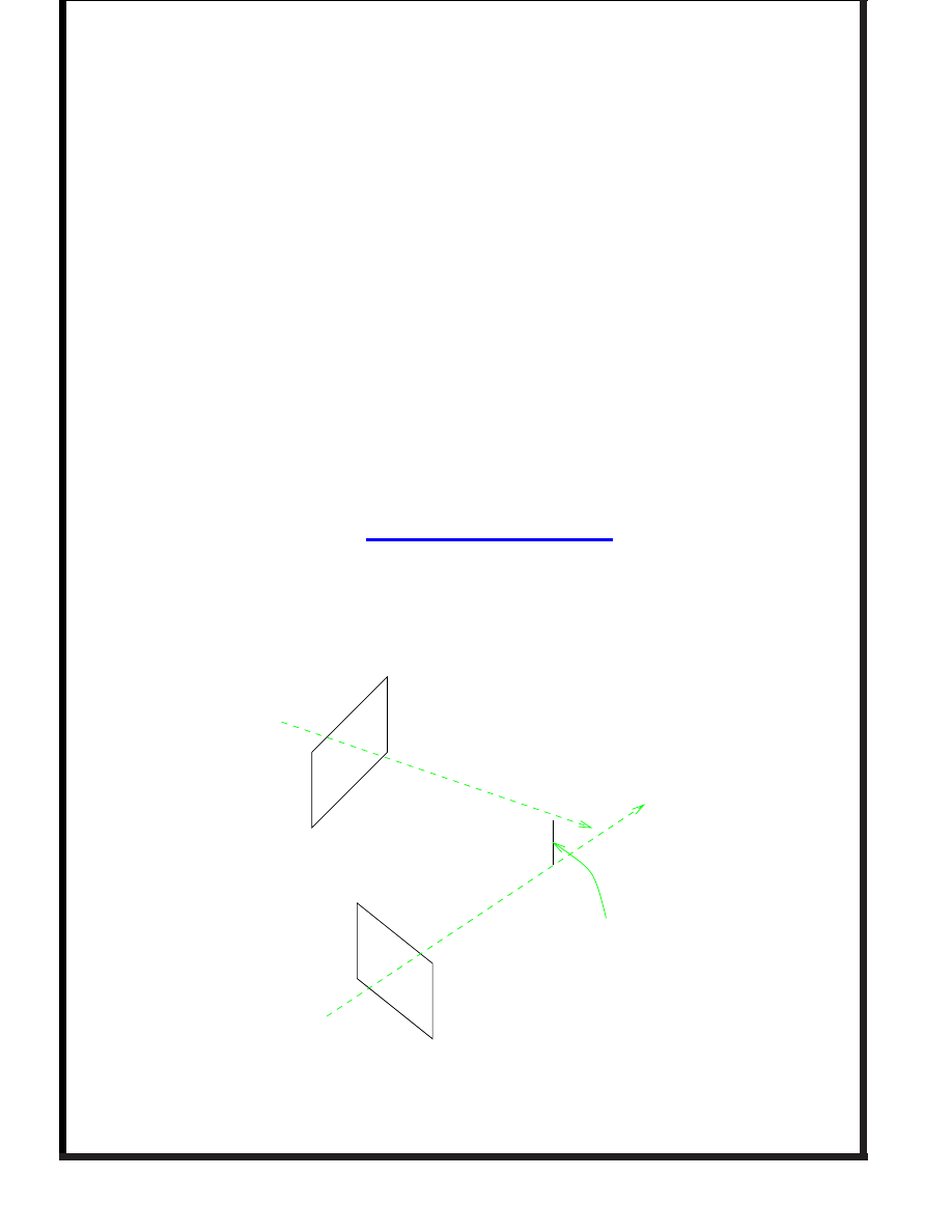
Has a simple

geometric

interpretation

Camera 1

Camera 2

Line Distance

Camera plane vectors extended out to 3-d space.

15

Find the rotor which minimises the squared distance

between

the lines

for each point match.

The setup is

scale-invariant

, so need to impose a scale. Do

this by fixing

with a Lagrange multiplier. Our final

function is

%

%

¼

%

%

¼

This is still quadratic in

and minimising gives the equation

We therefore construct the

symmetric

,

positive definite

function

This is a function of the data and the rotation only. The

translation is the eigenvector corresponding to the minimum

eigenvalue. This eigenvalue is

so the eigenvalue gives the error function. All need do is

minimise the lowest eigenvalue of

with respect to the rotor

. A fairly simple optimisation problem.

16

N

UMERICAL

R

ESULTS

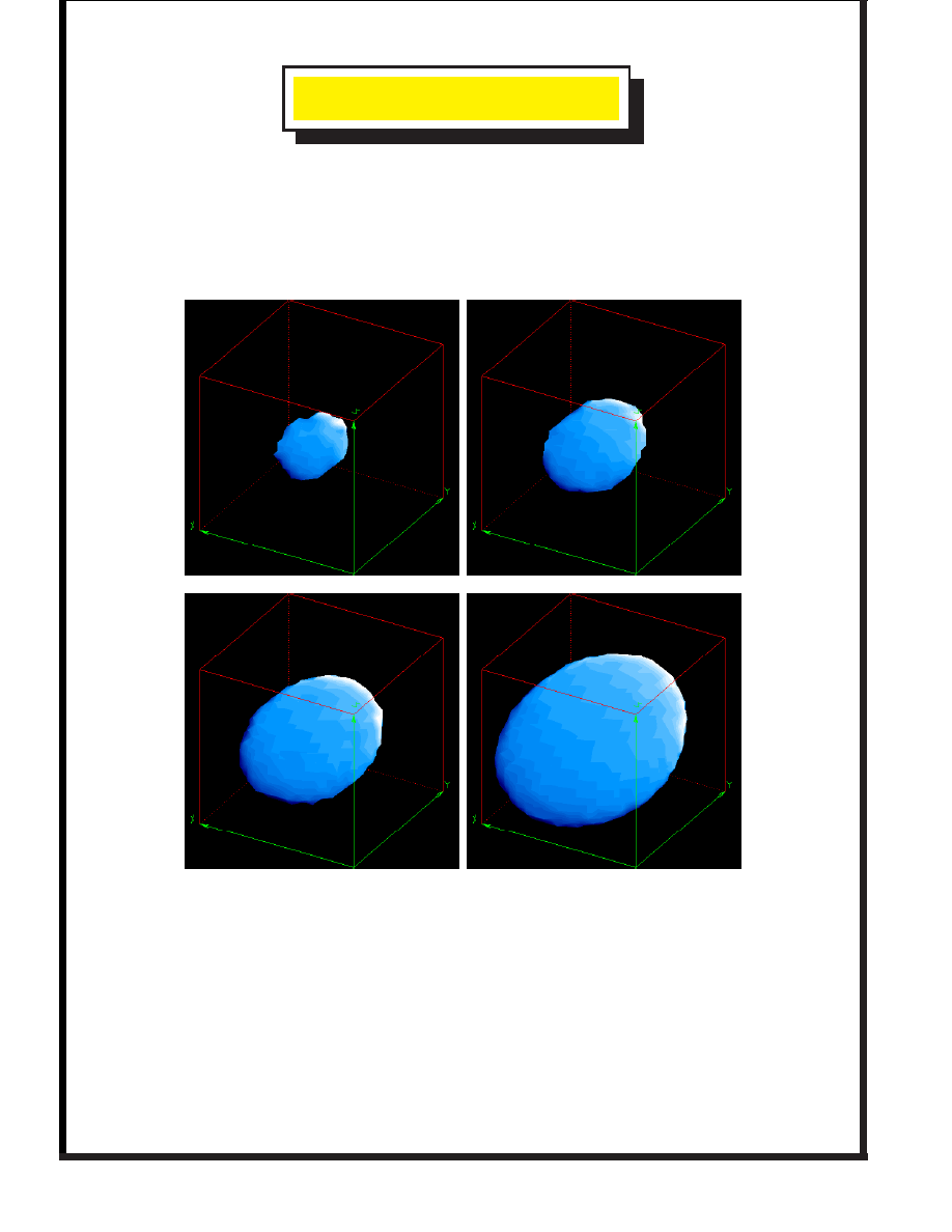
3-d contour plots of the function near the minimum look

reassuring:

The plots show surfaces of increasing

in the bivector space.

A clear trend towards a minimum. These plots used 8,000

function evaluations each. Each plots takes only

1 sec. on

a Pentium II.

17

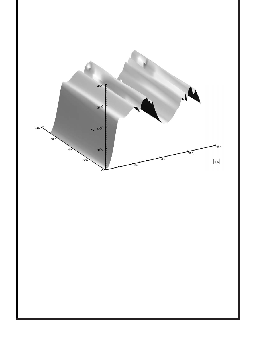
Small Problem

The function has a number of

local minima

. Downhill simplex

routines do not always find the global minimum. Need

annealing methods, or just use brute force.

Also see that function behaves very differently along direction

of rotation. From

¾

Suggests a number of potential improvements — e.g. reduce

to a 2-d function by minimising for angle.

18

E

XTENSION TO

C

AMERAS

Again this is easy. Can immediately write down an expression

to minimise for the translation vectors

Normalisation keeps everything symmetric. Now get three

equations

with the two constraints

The latter ensures that we still have

. Can recast as a

matrix equation of form

Hence find

. Again, look for best fit numerically.

19

C

ONCLUSIONS

1.

Geometric Algebra

is extremely powerful for handling

rotations in 3-d.

2.

Geometric Calculus

is extremely useful for extremisation

problems involving rotations.

3. Many computer vision problems best tackled by working

directly

with rotations and translations.

4. Auto-calibrating cameras for point matches with unknown

range data is not hard, even in the presence of noise.

5. The

Bayesian

derivation highlights the assumptions going

into the algorithms. Can change assumptions to model

noise better. Should give even better results

20