210Zboinski, Woznica art

Krzysztof Zboiński

Politechnika Warszawska

Piotr Woźnica

Politechnika Warszawska

THE UTILISATON OF ADVANCED VEHICLE

DYNAMICAL MODEL IN OPTIMISING THE SHAPE OF

RAILWAY TRANSITION CURVES

Abstract: This paper describes the concept and method by present authors of searching for
proper shape of transition curves. In the concept and the method the advanced dynamical
model of vehicle-track system, capable of simulation, and mathematically understood
optimisation methods are exploited. Principles and the most important details of the method are
obviously represented in the paper. They are supplemented with description of the software
built to solve the issue of transition curves formation (optimisation) effectively. At the end
results generated by this software are presented quite comprehensively.
Keywords: optimisation, numerical simulation, transition curves, railway vehicle dynamics,
track-vehicle interactions

1. INTRODUCTION

The problem discussed in present article is the search for proper shape of railway

transition curves. It is going to be done with regard to advanced vehicle model, dynamical
track-vehicle and vehicle-passenger interactions, and optimisation methods. The search for
proper shape means to the authors evaluation of the curve features based on chosen
dynamical quantities as well as the generation of such shape with use of mathematically
understood optimisation methods. The studies performed so far and those to be done in the
future have got a character of the numerical tests. The key element for these tests is use of
numerical simulation and the corresponding simulation software built by the authors. This
software enable to simulate dynamics of the vehicle-track system exploiting complete
dynamical model of the railway vehicle. Results of the simulations can be utilised in two
general ways. First is the direct use to get the complete knowledge about the dynamical
interactions and behaviour of the vehicle in transition curves. Second is the use of
simulation results to determine the objective function in the process of optimising the

shape of transition curve (TC). This second way of the results utilisation is discussed in the
paper first of all.

1.1. Short literature survey

Review of the literature given below cannot be complete in terms of the cited and

discussed publications since it would need a separate paper. Such a paper by present
authors is [1]. Below we discuss the literature jointly, trying to focus on the features being
the most common but not necessarily those most modern ones. Next, the criteria of TCs
evaluation are classified, which are used most often.

In opinion of present authors the most general classification of the works on TCs might

be their division into two groups. The first group includes those works that originate in the
issues of railway road design (construction). So, these works deal with the railway
infrastructure or in a wider view with the civil engineering. The second group is oriented
towards railway vehicle dynamics. Thus strong relation to the mechanical engineering is
clear. It seems that increase in total number of works concerning TCs that happened lately
[2, 3, 4, 5, 6, 7, 8, 9, 10, 11, 12] did not change a proportion between number of the works
in both groups. Despite increase in number of works in the second group
[11, 12, 13, 14, 15, 16, 17], the advantage of works' number in the first group is still a fact.

Recently increase in number of publications that deal with transition curves, both the

railway and the road ones, can be noticed. Also some qualitative change in their content
can be observed. It consists in attempts to diverge from the standard and to look for new,
more modern methods of evaluating properties of TCs. Despite these, some earlier visible
limitations of those works still exist, in present authors opinion. Namely, the analysis is
rather rare which takes account of advanced dynamics of whole vehicle-track system.
Present authors do not know method applied in practice (approved as a design tool), which
use complete dynamical model of vehicle in formation of railway TCs. Many of the
methods in use have got the traditional character. They are based on the traditional criteria
(discussed below) and often refer to very simple vehicle model. The authors failed to find
publications that exploit directly mathematically understood optimisation methods in
formation of TCs, basing on objective functions calculated as a result of the numerical
simulations. There are some works where selected quantities of interest, rather than the
shape of the curve itself, are optimised instead.

In many works from the first group approach to the track-vehicle interactions is

traditional, e.g. [18]. It is limited to discussing the vehicles jointly and studying the
selected effects (quantities) in the car body. In such works the fundamental criteria of 3-
dimensional TCs' formation are still crucial. Namely, the physical quantities that
characterise effects on the passenger and eventually on the cargo should not exceed values
that are acknowledged as acceptable [14, 18]. The corresponding relations refer to:
unbalanced lateral acceleration a

≤ a

lim

, velocity of the a change

≤

lim

, and velocity of

wheel vertical rise along the superelevation ramp f

≤ f

lim

. Some up-to-date works extend

these criteria with additional quantities and search for their courses. Such a quantity is the
second derivative of a with respect to time t or l, in case of constant v. As to the courses (of
the a first and second derivatives most often), the continuity (no abrupt change in values),
differentiability (no bends) and so on are demanded. Despite that extension, such criteria

do not take account of the dynamical properties of particular vehicle, including track-
vehicle interactions in particular conditions, or effects on vehicle bogie. These are different
than those adopted in the discussed criteria, where track has infinite stiffness and no
geometrical irregularities and vehicle is represented by a single rigid body or a particle.

Worthy of discussion are the criteria in the literature for evaluating TCs properties. Let

us classify them into tree groups called: geometrical, geodetic, and dynamic criteria. In
case of the geometrical criteria the appropriate boundary conditions at TC terminal points
must be satisfied [14, 18, 19]. Also so called consistency conditions inside TC have to be
satisfied. They ensure consistency (identity) of curvature k, superelevation ramp h, and
unbalanced acceleration a functions. Apart from the acceptable boundary and maximum
values also shape of the (da/dt)=

and sometimes d

a/dt

courses is of interest, e.g. [18].

The geodetic criteria compare different types of TCs from point of view of ease of their

setting down and maintenance during operation, e.g. [11, 20].

In case of the dynamical criteria [11, 12, 13, 14, 15, 16, 17] dynamical response of the

system on the input represented by TC (eventually including superelevation ramp) is of
interest. Two approaches can be distinguished here. The first is to build relatively simple
vehicle model that represents all vehicles and next to solve it analytically or numerically,
e.g. [13, 16, 20]. The second is to build advanced vehicle or vehicle-track model and to
solve it numerically (simulation) and then to analyse the results, e.g. [11, 12, 14, 15]. This
type of criteria and works in type of the last mentioned confirm us in a conviction that the
approach represented in our paper should be found justified and the results interesting.

2. AIMS AND SCOPE OF THE ARTICLE

2.1. The aim and scope in general

The main aim of the studies represented by present article is to elaborate and test the

numerical method of TCs form optimisation. This is in agreement with the general concept
of evaluating and forming TCs formulated in Sec. 1.

As to the scope, several introductory assumptions (expectations) have to be mentioned.

First, pure mathematical methods of optimisation are going to be used. Second, dynamical
quantities being the result of simulation of railway vehicle advanced (complete) model will
be used to determine the objective functions in the optimisation process. Third, possibility
of calculation a dozen or so different objective functions should be ensured in the software.
Forth, search for optimum solutions with objective functions based on traditional criteria
should be secured. Fifth, possibility to adopt all fundamental demands concerning TC
should be preserved in the software. Sixth, two-axle vehicle model as well as vertically and
laterally flexible track models are going to be used. Seventh, full non-linear geometry and
forces in wheel/rail contact have to be taken into account. Eight, polynomial TC is going to
be optimised. Ninth, the highest order of the polynomial should equal at least 12. Tenth,
optimisation of the entrance and exit TCs as well as of both simultaneously, for the
compound route, should be possible.

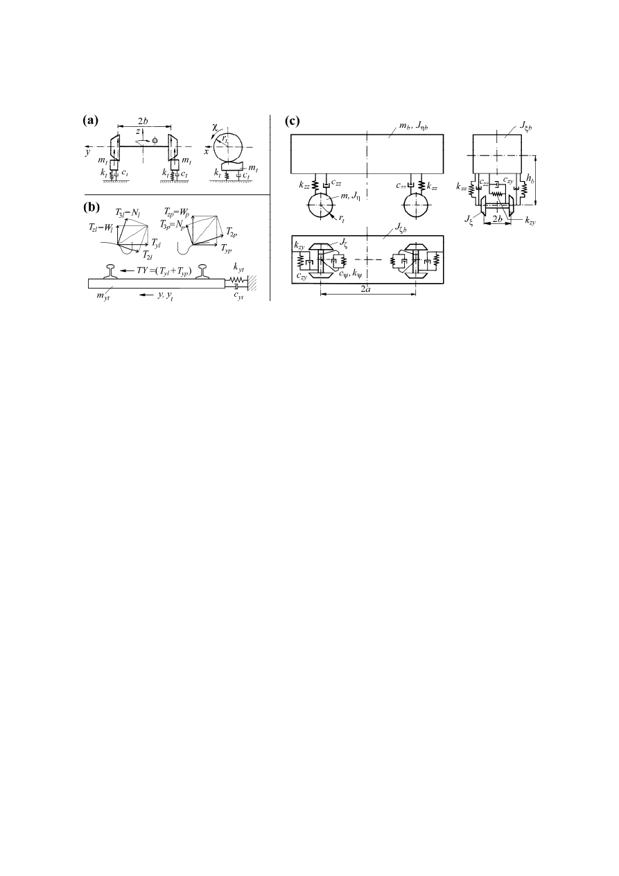
2.2. The object, its model, and the corresponding software

In order to make the analysis easier and more clear relatively simple object, and hence

its relatively simple model were utilised. To make direct reference to the earlier results
possible, the same model of the system was used as in the earlier studies by present authors
[14]. Consequently, all simulation studies were done for discrete vehicle model of 2-axle
freight car, as described in refs. [14, 21]. Its structure is shown in Fig. 1c. It is
supplemented with discrete models of vertically and laterally flexible track shown in
Figs. 1a and 1b, respectively. Parameters of the models are within average range of values
for 2-axle freight cars and for track, too. Linearity of the vehicle suspension system was
assumed. So, linear stiffness and damping elements in vehicle suspension were applied.
The same concerned the track models. Here also linear stiffness and damping elements
were utilised. One can find all parameters of the models in [14, 21].

Vehicle model is equipped with a pair of wheel/rail profiles that corresponds to the real

ones. That is a pair of the nominal (i.e. unworn) S1002/UIC60 profiles that are used all
over the Europe. Non-linear geometry of this pair is introduced into the model in a form of
the table with contact parameters. In order to calculate non-linear tangential contact forces
between wheel and rail well known FASTSIM program by J.J. Kalker was applied. Normal
forces in the contact are not constant but influenced by both the geometry and the
dynamical effects influencing value of a wheelset vertical load.

Generalised approach to the modelling was used, as explained in [21, 22, 23]. Basically,

dynamics of relative motion is used in that approach. This means that description of
motion (dynamics) is relative to track-based moving reference frames. Dynamical
equations of motion are equations of relative motion with terms depending on motion of
the reference frames explicitly recorded. None of such terms is omitted in the equations.
According to this method, the kinematic type non-linearities arising from rotational
motions of bodies within our MBS model are taken into account, too. The term generalised
refers fist of all to the generalised conditions of motion. So, the same generalised vehicle
model describes vehicle dynamics in any conditions, i.e. in straight track (ST), circular
curve (CC), and TC sections. The routes composed of such sections can also be analysed.

The route (section) of interest is characterised in the method by shape of the track centre

line which is the general space (3-dimensional) curve. In railway systems such 3-
dimensional objects are TCs with their superelevation ramps. A necessary condition to

apply the method is description of the curves (sections) by parametric equations, with the

Fig. 1. System's nominal model: (a) track vertically, (b) track laterally, (c) vehicle

curve's current length as the parameter. The cases of CC and ST are treated in the method
as the special cases of 2-dimensional and 1-dimensional geometrical objects, respectively.
Such an approach was described in [19, 23].

An important element in the method is description of kinematics of the track-based

moving reference frames. Their motion comes out directly from the track centre line shape.
The applied method of determination of the kinematical quantities on the basis of the
parametric equations is presented most recently in [23].

3. METHOD FOR OPTIMUM TRANSITION CURVE FORMATION

3.1. The simulation software

Simulation software reflects in numerical form all the features specified above for the
mathematical model. So, the original as well as characteristic features of the model are
represented in the software. Despite many such features, in general view our software
might be defined as a typical railway vehicle dynamics simulation software. We mean that
the aims for its use and results generated are those typical.
The software in view was built by the authors on their own, so it is not a commercial
code. It is also not a software for automatic generation of equations of motion (AGEM) but
the one corresponding to a particular mechanical system. Here it corresponds to the system
defined in Fig. 1. It was developed, tested, and used in research for many years. The base
in this software is set of the 2nd order ordinary differential equations (ODEs). These
equations of motion were derived from Lagrange equations of type II adapted to
description of relative motion. General form of such equations is presented in [19, 21].
Number of the equations equals a number of degrees of freedom (DOFs) of the system.
Complete vehicle-track system possess 18 DOFs. The equations of 2nd order are
transformed within the code into the 1st order ODEs to integrate them. The integration is
done with use of methods capable to solve stiff differential equations (Gear's methods).

Direct result of the numerical integration are obviously the system co-ordinates and
velocities. Apart from them, the broad set of other supplementary quantities can also be
obtained. For example these could be forces and torques exploited in the simulations. The
results can either be recorded in the resultant files or used directly in the calculations. Both
the direct and the supplementary results are used while calculating values of objective
functions during the optimisation.

3.2. Type of the transition curve and conditions for it

Type of a TC chosen for optimisation is the polynomial TC of any order n

≥4. It is defined

by Eqs. (1)-(4) that are related to space curve parametric equations:

⎟⎟

⎠

⎞

⎜⎜

⎝

⎛

−

.....

(1)

⎟⎟

⎠

⎞

⎜⎜

⎝

⎛

⋅

−

.....

)

)(

(

)

(

(2)

⎟⎟

⎠

⎞

⎜⎜

⎝

⎛

⋅

−

.....

)

)(

(

)

(

(3)

⎟⎟

⎠

⎞

⋅

⎜⎜

⎝

⎛

−

.....

)

)(

(

)

)(

(

(4)

where y, k, h, and i define curve lateral co-ordinate, curvature, superelevation, and
inclination of superelevation ramp, respectively. The R, H, L, and l define curve minimum
radius (at its end), maximum susperelevation (at the curve end), total curve length, and
current curve length, respectively. The A

are polynomial coefficients (i=n, n-1,…., 4, 3)

while n is polynomial order. Number of the polynomial terms (terms in Eqs. (1)-(4)) must
not be smaller than 2. Definition of the curves as adopted here gives possibility of proper k
and h values at TCs terminal points. They should equal 0 at the initial points and 1/R and H
at the end points. Note, that values for both always equal 0 for l=0. In order to ensure 1/R
and H values for l=L, normalisation of the coefficients is necessary. It is done with WSR
coefficient defined in Eq. (5). The normalised coefficients A'

are given in Eq. (6).

(

)

(

)

⋅

−

⋅

−

WSR

.....

)

)(

(

)

(

)

(

.....

)

)(

(

)

(

(5)

WSR

′

−

..........

.......

(6)

Finally, form of each TC being tested for optimum shape during the optimisation process is
determined with the following parametric equations:

⎟⎟

⎠

⎞

⎜⎜

⎝

⎛

⋅

−

⎟⎟

⎠

⎞

⎜⎜

⎝

⎛

′

≅

−

.....

)

)(

(

)

(

.......

(7)

In order to ensure tangence of the k and h functions at their terminal points to the k and h
functions for ST and CC, values of i function given in Eq. (4) should equal 0 for l=0 and
l=L. Equation (4) always produce 0 for l=0 when its last term is removed. An this is the
first condition that affects also rest of the equations. To ensure 0 value for l=L the round
bracket in (4) with the last term omitted should equal 0. In order to make it true all the
coefficients remain unchanged but not just one arbitrarily selected. Its value is taken as
opposite to the sum of those unchanged. And this is the second condition, that affects also
rest of the equations. In case the second coefficient is selected for change it would be:

(

)

′

⋅

′

⋅

′

−

′′

⎟⎟

⎠

⎞

′

⋅

⎜⎜

⎝

⎛

′

−

′

−

.....

)

)(

(

)

)(

(

.....

)

)(

(

)

)(

(

(8)

Some problem in optimising form of TC is a starting point (initial form of TC). In case

of TC of 5th, 7th, and 9th orders we used the curves known in the literature as the best
ones from point of view of the traditional criteria. For example, in case of the 5th order it
was the Bloss (Glodner) curve. Generally, such curves ensure minimum of the centrifugal
force integral inside a TC. This is satisfied for the simplest possible model, however, that is
in fact represented by a particle. For the higher order polynomial TCs form of the initial
TC was an arbitrary choice, possibly in connection with TCs found in the literature. The
curves in view are given below.

⎟⎟

⎠

⎞

⎜⎜

⎝

⎛

−

(9)

⎟⎟

⎠

⎞

⎜⎜

⎝

⎛

−

(10)

⎟⎟

⎠

⎞

⎜⎜

⎝

⎛

−

(11)

3.3.Optimisation method and objective functions

Let us formulate the optimisation problem that is going to be solved in the presented

studies. So, one ought to find A'

, being the polynomial coefficients, ensuring possibility of

imposing constraints on their values. The constraints in the form b

<A'

should enable to

control form of the polynomials in case it is necessary. Namely, the forms of polynomials
reasonable from practical point of view should be tested in succeeding steps of the
optimisation process, rather than those being impossible to apply in a railway conditions.
The problem just formulated is a classical formulation of the static constrained
optimisation. It is realised with the library procedure that utilises moving penalty function
algorithm combined with Powell's method of conjugate directions.

The difficulty of the problem solution lies in the very complex objective function

(quality function). This function is calculated as a result of the numerical simulation of
dynamical mechanical system (as described in Subsecs. 3.2 and 4.1). The main steps
during calculation of the objective function are: generation of the new shape of TC,
calculation of kinematical quantities (velocities and accelerations) that depend on this new
shape, and solution of ODEs set.

At current stage of the studies nine quality functions (QF) were implemented in the

software. They concern minimisation of: sum of lateral displacements for both wheelsets
(QF

); sum of squares of longitudinal and lateral creepages in wheel/rail contact for all

wheels (QF

); sum of yaw angles for both wheelsets (QF

); wheel/rail wear represented by

sum of products of tangential forces by creepages in longitudinal and lateral directions for
all wheels (QF

); wheel/rail wear represented by sum of products of normal forces and

resultant creepages for all wheels (QF

); sum of normal forces for all wheels (QF

); sum of

lateral accelerations of wheelsets and car body (QF

); sum of lateral accelerations of

wheelsets (QF

); and lateral acceleration of car body (QF

So far just three functions were tested. They are QF

, QF

, and QF

. Their physical

interpretation is as follows. Minimisation of QF

causes less wear of wheels and rails, of

reduces vehicle-track and vehicle-passenger interactions, while of QF

reduces

vehicle-track interactions. These three QFs are given in Eqs. (12), (13), and (14):

(

)

yrk

xrk

ylk

xlk

xrp

ylp

xlp

∫

−

(12)

(

)

∫

−

(13)

(

)

∫

−

(14)

where L

is distance where QF is calculated,

is longitudinal creepage,

is lateral

creepage, and

y&&

is lateral acceleration. Indices l, r, p, k, b refer to left hand-side, right

hand-side, leading wheelset, trailing wheelset, and vehicle body, respectively.

3.4. General representation of the software

Scheme of the software is shown in Fig. 2. Two iteration loops are visible there. The

first is an integration loop. This loop is stopped when distance l

lim

being length of the route

(usually the compound route ST, TC, and CC) is reached by vehicle model. The second is
an optimisation process loop. It is stopped when number of iterations reaches limit value
i

lim

. This value means that i

lim

simulations have to be performed in order to stop

optimisation process. In the calculations done so far i

lim

equal 100 was used. If optimum

solution is reached earlier, i.e. for i<i

lim

then the optimisation process stops automatically

and the corresponding results are recorded. The post-processor ensures record of A'

coefficients in each optimisation step in the special file. Besides results of simulations for
the initial and optimum TC shapes are recorded automatically in the resultant files.

Fig. 2. General scheme of the optimisation software

4. RESULTS OF NUMERICAL TESTS

The results to be presented are divided into two parts. The aim for the first part is

demonstration that the method works well and results of optimisations will be useful in the
future analyses. The aim for the second part is to show what kind of results can be

generated and how the first analyses look like. All the results below refer to the same
compound route. Its data are: velocity v=45 m/s, (ST; L=50 m), (TC; L=102,5 m, R

min

=600

m, H

max

=0,16 m), (CC; L=100 m, R=600 m, H=0,16 m).

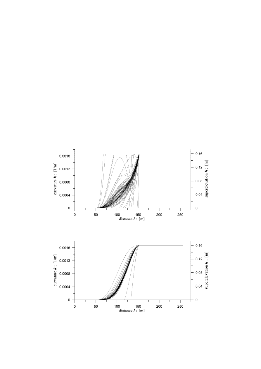
4.1. Results Aimed at testing the Software

It can be seen from Figs. 3 and 4 that searching for the optimum TC is successful.

Usually quite wide range of the shapes is swept (tested). It can be seen in Figs. 3 and 4 that
applied method of forcing the software to take proper values for k and h at TC's terminal
points works right. By comparing these figures it can also be seen that the method ensuring
tangence of k and h functions for TC at its terminal points to the functions for ST and CC
works right, too. It can be observed for the shapes producing k and h values smaller than 0
or higher than 1/R and H that such values are trimmed off by the software to avoid model's
"derailment". In case "derailment" persists, QFs are given very high values to stop interest
of the software in such solutions. Coefficients A'

for the optimised TCs are given in Sec. 6.

Fig. 3. Search for optimum 7th order TC's shape, represented by curvature k and superelevation h. No

conditions for the tangence of the k and h is imposed. QF

is used

Fig. 4. Search for optimum 7th order TC's shape represented by curvature k and superelevation ramp.

Condition for the tangence of the k and h is imposed. QF

is used

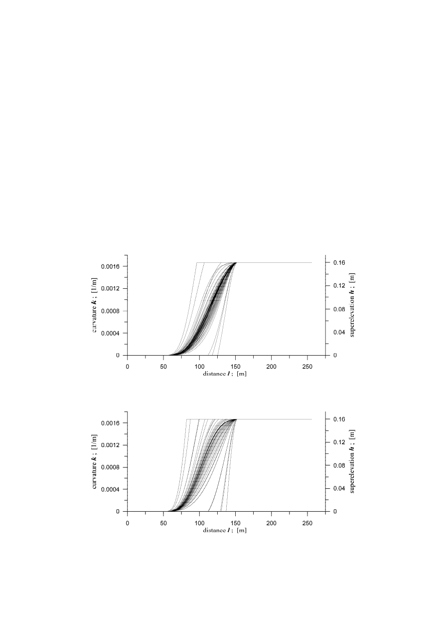
4.2. Results of Optimisation and Dynamical Simulations

It can be seen in Figs. 5 and 6 that for different QFs optimisation process goes

differently. Different sets of the curves are tested for being or not the optimum ones.
Obviously different sets of A'

coefficients for optimum shapes are obtained (see Sec. 6),

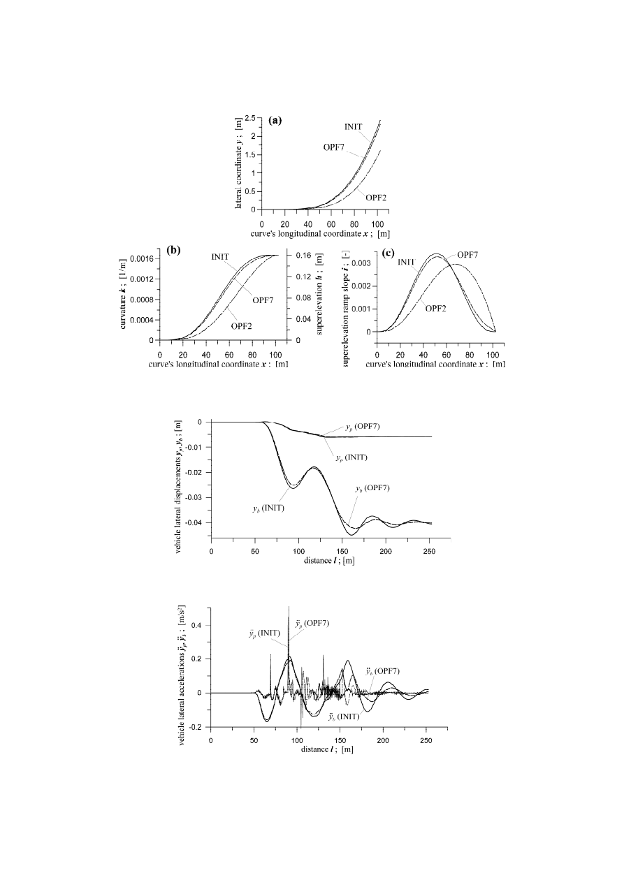
too. Figure 7 represents optimised shape of the curves and features for such curves.
Figure 7(a) represents the shapes in plane while Fig. 7(b) the shape of superelevation
ramps. Basic features of the curves are shown in Figs. 7(b) and 7(c). Figure 7(c) shows
curvatures and Fig 7(c) shows superelevation ramp slopes. Denotations used in these
figures are OPF2, OPF7, and INIT for QF

, QF

quality functions, and for the initial shape

given with Eq. (11), respectively. Figs. 8 and 9 represent selected dynamical quantities that
show improvement in the vehicle dynamical behaviour due to use of the optimised TC
shape. Comparison for the initial (INIT) and the optimised (OPF7) curves is done there.
Despite relatively small differences in these curves shapes and in their features seen in
Fig. 7, the improvements revealed in Figs. 8 and 9, especially for the car body, are
spectacular. Differences for the wheelsets also exist but are much smaller.

Fig. 5. Search for optimum 9th order TC's shape represented by curvature k and superelevation ramp.

Condition for the tangence of the k and h is imposed. QF

is used.

Fig. 6. Search for optimum 7th order TC's shape represented by curvature k and superelevation ramp.

Conditions for the tangence of the k and h is imposed. QF

is used.

Fig.7. Results of optimisation for QF

and QF

compared to the initial curve: (a) curve shapes, (b) curvatures

and supelevations, (c) superelevation ramp slopes

Fig. 8. Vehicle model lateral displacements for optimised (QF

) and initial TCs

Fig. 9. Vehicle model lateral accelerations for optimised (QF

) and initial TCs

5. CONCLUSION

The idea and the corresponding software presented in current paper appeared to be

effective tool in optimising polynomial TCs form. It proved true for different quality
functions based on the dynamical quantities from the advanced vehicle-track system. It
was possible to generate A'

polynomial coefficients in all case studies done so far. The sets

of coefficients corresponding to TCs optimised in present paper, recorded from the highest
to the lowest order of the terms, are as follows: Fig. 3, {0.19999, -0.49975, 0.37363}; Fig.
4, {1.3015, 2.4063, –0.26081, 0.0081477}; Fig. 5, {-0.26498, 1,3646, -2.736, 2.0801}; Fig.
6, {-0.28031, 1.25, -1.9939, 1.1667}. Number of the terms depends on the data taken
before each optimisation. To get the TCs' equations, the above coefficients have to be
introduced into Eq. (7).
It was shown that TCs properties can be improved by omission the lowest order terms.
The example are superelevation slopes (inclinations) in Fig. 7c. The TC matching OFP2
curve has one term less than TCs matching OFP7 and INIT curves.

In the foreseeable future the following issues deserve our attention. More QFs should be

tested and proposed. Some could take account of the several factors with use of the
weighting factors, some could be calculated for the selected parts of TCs. Next,
optimisations for the exit TCs and for the routes that include both the entrance and exit
TCs would be desirable. Our software is capable of doing these. Number of the case
studies necessary to perform in order to recommend any optimum TC shape for practice is
really large.

Acknowledgement

Scientific work financed as research project no. N N509 403136 in the years 2009-2011 from funds
for science of Ministry of Science and Higher Education, Warsaw, Poland.

References

1. Woźnica P., Zboiński K.: Analiza literatury krajowej i swiatowej dotyczącej modelowania krzywych

przejściowych z naciskem na metody komputerowe. ILiM, Logistyka, nr 6, 2009, CD Logistyka –
nauka; Railway Transport (CD jest integralną częścią wydania 6/2009 – zastrzeżenie radakcji).

2. O. Baykal, “Concept of Lateral Change of Accelaration”, Journal of Surveying Engineering, 122(3),

132-140, 1996.

3. E. Tari, O. Baykal, “A New Transition Curve with Enhanced Properties”, Canadian Journal of Civil

Engineering, 32(5), 913-923, 2005.

4. A. Ahmad, J. Ali, “G

Transition Curve Between Two Straight Lines”, Proc. 5

CGIV’08, 154-159,

IEEE Computer Society, New York, 2008.

5. Y. Tanaka, “On the Transition Curve Considering Effect of Variation of the Train Speed”, ZAMM – J.

of Aapplied Mathematics and Mechanics, 15(5), 266-267, 2006.

6. A. Ahmad, R. Gobithasan, J. Md. Ali, “G2 Transition Curve Using Quadratic Bezier Curve”, in

“Proceedings of the Computer Graphics, Imaging and Visualisation Conference”, 223-228, IEEE
Computer Society, 2007.

7. Z. Li, L. Ma, M. Zhao, Z. Mao, “Improvement Construction for Planar G

Transition Curve Between

Two Separated Circles, in V. N. Alexandrov et al. (Editors), ICCS 2006, Part II, LNCS 3992, 358-361,
2006.

8. Z. Habib, M. Sakai, “G

Planar Cubic Transition Between Two Circles”, International Journal of

Computer Mathematics, 80(8), 957-965, 2003.

9. S. Fischer, “Comparison of Railway Track Transition Curves Types”, Pollack Periodica - An

International Journal for Engineering and Information Sciences, 4(3), 99-110, 2009.

10. E. Tari, O. Baykal, ”An Alternative Curve in The Use of High Speed Transportation System”, ARI - An

International Journal For Physical and Engineering Sciences, 51, 126-135, 1998.

11. X.Y. Long, Q.C. Wei, F.Y. Zheng, “Dynamic Analysis of Railway Transition Curves”, Proc IMechE,

Part F: Journal of Rail and Rapid Transit, 224(1), 2010, DOI 10.1243/09544097JRRT287.

12. B. Kuvfer, “Optimization of Horizontal Alignments for Railway – Procedure Involving Evaluation of

Dynamic Vehicle Response”, Ph.D. Thesis, Royal Institute of Technology, Stockholm, 2000.

13. W. Koc, E. Mieloszyk, The Comparing Analysis of Some Transition Curves Using the Dynamic Model”,

Archives of Civil Engineering, 33(2), 239-261, 1987.

14. K. Zboinski, “Numerical Studies on Railway Vehicle Response to Transition Curves with Regard to

Their Different Shape”, Archives of Civil Engineering, XLIV(2), 151-181, 1998.

15. J. Drozdziel, B. Sowinski, “Railway Car Dynamic Response to Track Transition Curve and Single

Standard Turnout”, in “Computers in Railways X”, J. Allan et.al. (Editors), 849-858, WIT Press 2006.

16. J. Pombo, J. Ambrosio, “General Spatial Curve Joint for Rail Guided Vehicles:Kinematics and

Dynamics”, Multibody System Dynamics, 9(3), 237-264, 2003.

17. B. Kufver, J. Forstberg, “Dynamic Vehicle Response Versus Virtual Transitions”, Computers in

Railways IX, WIT Press, 799-807, 2004.

18. Esveld C., “Modern Railway Track”, MRT-Productions, Duisburg 1989.
19. K. Zboinski, “Railway Vehicle-Track Model in Its General Conception”, in “Advanced Railway Vehicle

System Dynamics”, J. Kisilowski, K. Knothe, (Editors), WNT – Science and Technology Publishers,
Warsaw, Poland, 29-56, 1991.

20. W. Koc, "Transition Curves with Nonlinear Superelevation Ramps in Exploitation Conditions of PKP",

Scientific Bulletins of Gdańsk University of Technology - Civil Engineering, 47, 1990.

21. K. Zboinski, “Importance of Imaginary Forces and Kinematic Type Nonlinearities for Description of

Railway Vehicle Dynamics”, Proceedings of the Institution of Mechanical Engineers, part F, Journal of
Rail and Rapid Transit, 213(4), 199-210, 1999.

22. K. Zboinski, “Relative Kinematics Exploited in Kane’s Approach to Describe Multibody Systems in

Relative Motion”, Acta Mechanica, 147(1-4), 19-34, 2001

23. K. Zboinski, “Numerical and traditional modelling of dynamics of multi-body system in type of a

railway vehicle”, Archives of Transport, 16(3), 81-106, 2004.

WYKORZYSTANIE ZAAWANSOWANEGO MODELU DYNAMICZNEGO POJAZDU

W OPTYMALIZACJI KSZTAŁTU KOLEJOWYCH KRZYWYCH PRZEJŚCIOWYCH

Streszczenie: Niniejszy artykuł opisuje koncepcję i metodę poszukiwania właściwego kształtu
kolejowych krzywych przejściowych. W koncepcji oraz metodzie wykorzystuje się
zaawansowany model dynamiczny układu tor-pojazd, z możliwością symulacji, oraz
matematycznie rozumiane metody optymalizacji. Oczywiście w artykule przedstawiono
podstawy jak i najważniejsze szczegóły metody. Są one uzupełnione o opis oprogramowania
zbudowanego dla efektywnego rozwiązania zagadnienia kształtowania (optymalizacji)
krzywych przejściowych. Na koniec, całkiem obszernie przedstawione zostały wyniki
generowane przez oprogramowanie.
Słowa kluczowe: optymalizacja, symulacja numeryczna, krzywe przejściowe, dynamika
pojazdów szynowych, oddziaływania tor-pojazd

Wyszukiwarka

Podobne podstrony:
(Art 98 a 100)
ART
Art & Intentions (final seminar paper) Lo
art 10 1007 s00482 013 1385 z
Koscioly nie majace własnej hierarchii - art
Kolorowy art jakby gazetowy
art DS 10( list bud
Art&8
Wpływ TV na dzieci! (art z sieci)
Art
art DS 10' wrze
Kodeks Dobra osobiste Art# i$
[2001] State of the Art of Variable Speed Wind turbines
535 0a56c Art 10 orto 04 08 czamara

więcej podobnych podstron