Coupled Structural/Thermal Analysis

Introduction

This tutorial was completed using ANSYS 7.0 The purpose of this tutorial is to outline a simple coupled

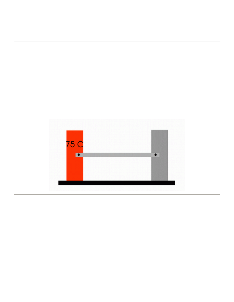
thermal/structural analysis. A steel link, with no internal stresses, is pinned between two solid structures at a
reference temperature of 0 C (273 K). One of the solid structures is heated to a temperature of 75 C (348 K). As

heat is transferred from the solid structure into the link, the link will attemp to expand. However, since it is
pinned this cannot occur and as such, stress is created in the link. A steady-state solution of the resulting stress
will be found to simplify the analysis.

Loads will not be applied to the link, only a temperature change of 75 degrees Celsius. The link is steel with a

modulus of elasticity of 200 GPa, a thermal conductivity of 60.5 W/m*K and a thermal expansion coefficient of
12e-6 /K.

Preprocessing: Defining the Problem

According to Chapter 2 of the ANSYS Coupled-Field Guide, "A sequentially coupled physics analysis is the
combination of analyses from different engineering disciplines which interact to solve a global engineering
problem. For convenience, ...the solutions and procedures associated with a particular engineering discipline

[will be referred to as] a physics analysis. When the input of one physics analysis depends on the results from
another analysis, the analyses are coupled."

Thus, each different physics environment must be constructed seperately so they can be used to determine the

coupled physics solution. However, it is important to note that a single set of nodes will exist for the entire
model. By creating the geometry in the first physical environment, and using it with any following coupled

environments, the geometry is kept constant. For our case, we will create the geometry in the Thermal
Environment, where the thermal effects will be applied.

University of Alberta ANSYS Tutorials - www.mece.ualberta.ca/tutorials/ansys/AT/Coupled/Coupled.html

Copyright © 2001 University of Alberta

Although the geometry must remain constant, the element types can change. For instance, thermal elements are
required for a thermal analysis while structural elements are required to deterime the stress in the link. It is

important to note, however that only certain combinations of elements can be used for a coupled physics
analysis. For a listing, see Chapter 2 of the ANSYS Coupled-Field Guide located in the help file.

The process requires the user to create all the necessary environments, which are basically the preprocessing

portions for each environment, and write them to memory. Then in the solution phase they can be combined to
solve the coupled analysis.

Thermal Environment - Create Geometry and Define Thermal Properties

1. Give example a Title

Utility Menu > File > Change Title ...

/title, Thermal Stress Example

2. Open preprocessor menu

ANSYS Main Menu > Preprocessor

/PREP7

3. Define Keypoints

Preprocessor > Modeling > Create > Keypoints > In Active CS...

K,#,x,y,z

We are going to define 2 keypoints for this link as given in the following table:

4. Create Lines

Preprocessor > Modeling > Create > Lines > Lines > In Active Coord

L,1,2

Create a line joining Keypoints 1 and 2, representing a link 1 meter long.

5. Define the Type of Element

Preprocessor > Element Type > Add/Edit/Delete...

For this problem we will use the LINK33 (Thermal Mass Link 3D conduction) element. This
element is a uniaxial element with the ability to conduct heat between its nodes.

6. Define Real Constants

Preprocessor > Real Constants... > Add...

In the 'Real Constants for LINK33' window, enter the following geometric properties:

i. Cross-sectional area AREA: 4e-4

This defines a beam with a cross-sectional area of 2 cm X 2 cm.

Keypoint Coordinates (x,y,z)
1

(0,0)

2

(1,0)

University of Alberta ANSYS Tutorials - www.mece.ualberta.ca/tutorials/ansys/AT/Coupled/Coupled.html

Copyright © 2001 University of Alberta

7. Define Element Material Properties

Preprocessor > Material Props > Material Models > Thermal > Conductivity > Isotropic

In the window that appears, enter the following geometric properties for steel:

i. KXX: 60.5

8. Define Mesh Size

Preprocessor > Meshing > Size Cntrls > ManualSize > Lines > All Lines...

For this example we will use an element edge length of 0.1 meters.

9. Mesh the frame

Preprocessor > Meshing > Mesh > Lines > click 'Pick All'

10. Write Environment

The thermal environment (the geometry and thermal properties) is now fully described and can be
written to memory to be used at a later time.

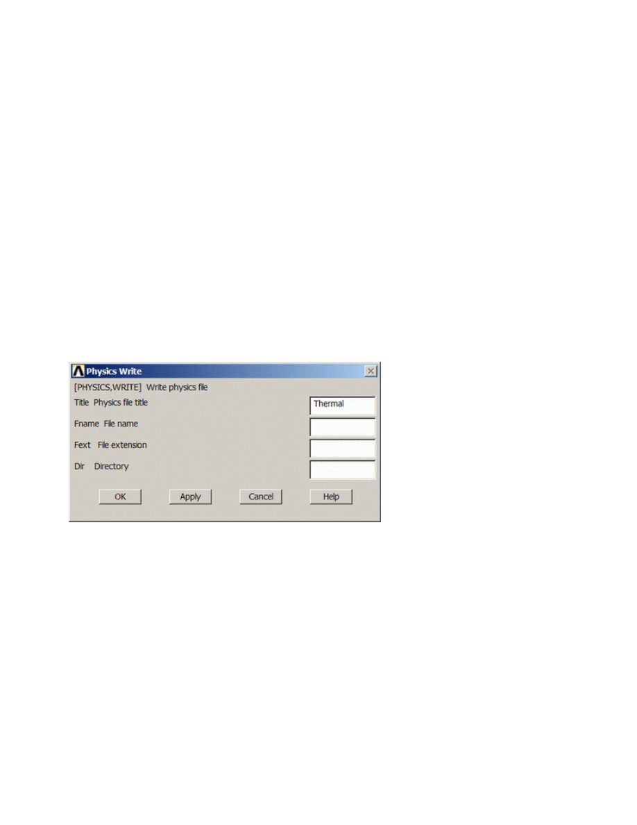
Preprocessor > Physics > Environment > Write

In the window that appears, enter the TITLE Thermal and click OK.

11. Clear Environment

Preprocessor > Physics > Environment > Clear > OK

Doing this clears all the information prescribed for the geometry, such as the element type, material
properties, etc. It does not clear the geometry however, so it can be used in the next stage, which is
defining the structural environment.

Structural Environment - Define Physical Properties

Since the geometry of the problem has already been defined in the previous steps, all that is required is to detail

the structural variables.

1. Switch Element Type

Preprocessor > Element Type > Switch Elem Type

Choose Thermal to Struc from the scoll down list.

University of Alberta ANSYS Tutorials - www.mece.ualberta.ca/tutorials/ansys/AT/Coupled/Coupled.html

Copyright © 2001 University of Alberta

This will switch to the complimentary structural element automatically. In this case it is LINK 8.
For more information on this element, see the help file. A warning saying you should modify the

new element as necessary will pop up. In this case, only the material properties need to be modified
as the geometry is staying the same.

2. Define Element Material Properties

Preprocessor > Material Props > Material Models > Structural > Linear > Elastic > Isotropic

In the window that appears, enter the following geometric properties for steel:

i. Young's Modulus EX: 200e9

ii. Poisson's Ratio PRXY: 0.3

Preprocessor > Material Props > Material Models > Structural > Thermal Expansion Coef >

Isotropic

i. ALPX: 12e-6

3. Write Environment

The structural environment is now fully described.
Preprocessor > Physics > Environment > Write

In the window that appears, enter the TITLE Struct

Solution Phase: Assigning Loads and Solving

1. Define Analysis Type

Solution > Analysis Type > New Analysis > Static

ANTYPE,0

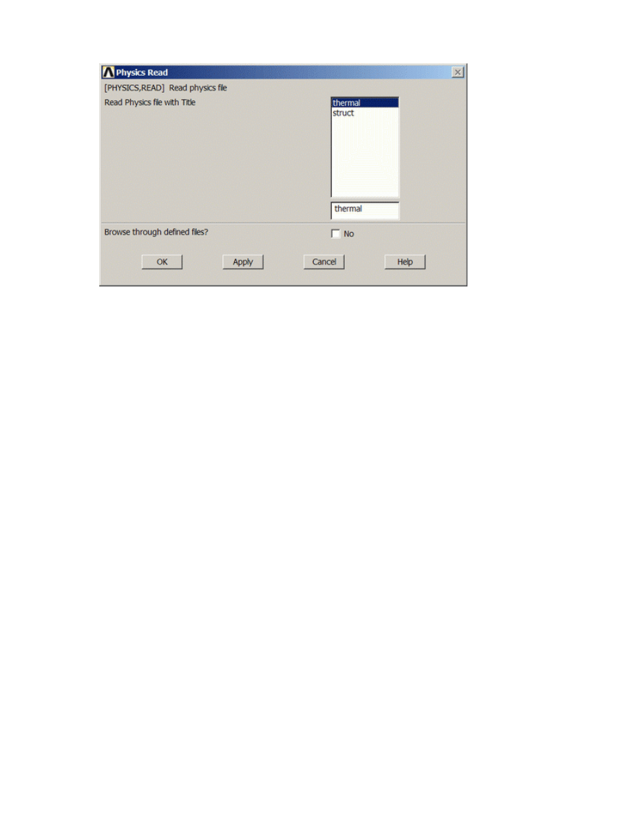
2. Read in the Thermal Environment

Solution > Physics > Environment > Read

Choose thermal and click OK.

University of Alberta ANSYS Tutorials - www.mece.ualberta.ca/tutorials/ansys/AT/Coupled/Coupled.html

Copyright © 2001 University of Alberta

If the Physics option is not available under Solution, click Unabridged Menu at the bottom of the

Solution menu. This should make it visible.

3. Apply Constraints

Solution > Define Loads > Apply > Thermal > Temperature > On Keypoints

Set the temperature of Keypoint 1, the left-most point, to 348 Kelvin.

4. Solve the System

Solution > Solve > Current LS

SOLVE

5. Close the Solution Menu

Main Menu > Finish

It is very important to click Finish as it closes that environment and allows a new one to be opened

without contamination. If this is not done, you will get error messages.

The thermal solution has now been obtained. If you plot the steady-state temperature on the link, you will
see it is a uniform 348 K, as expected. This information is saved in a file labelled

Jobname.rth

, were .rth

is the thermal results file. Since the jobname wasn't changed at the beginning of the analysis, this data can
be found as file.rth. We will use these results in determing the structural effects.

6. Read in the Structural Environment

Solution > Physics > Environment > Read

Choose struct and click OK.

7. Apply Constraints

Solution > Define Loads > Apply > Structural > Displacement > On Keypoints

Fix Keypoint 1 for all DOF's and Keypoint 2 in the UX direction.

University of Alberta ANSYS Tutorials - www.mece.ualberta.ca/tutorials/ansys/AT/Coupled/Coupled.html

Copyright © 2001 University of Alberta

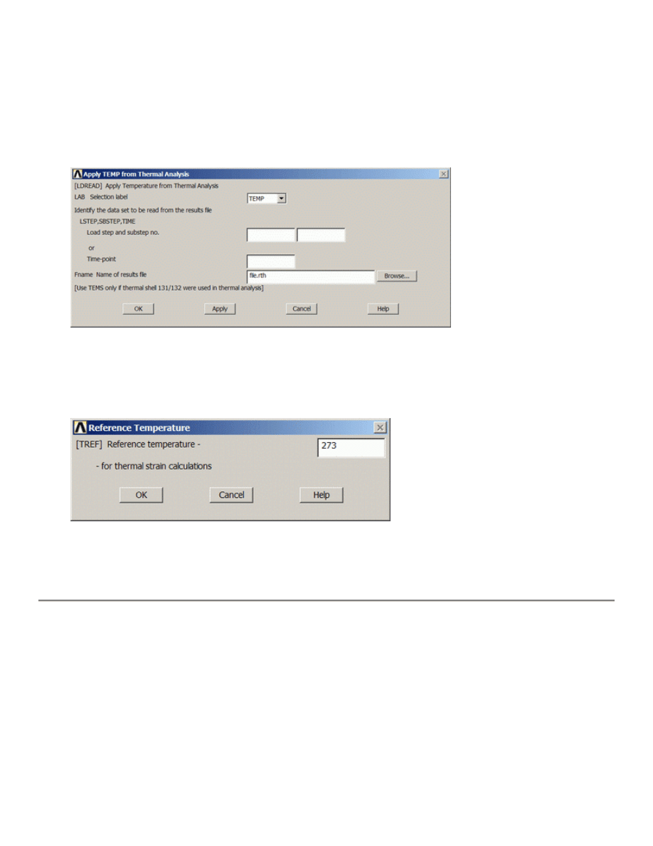
8. Include Thermal Effects

Solution > Define Loads > Apply > Structural > Temperature > From Therm Analy

As shown below, enter the file name

File.rth

. This couples the results from the solution of the

thermal environment to the information prescribed in the structural environment and uses it during
the analysis.

9. Define Reference Temperature

Preprocessor > Loads > Define Loads > Settings > Reference Temp

For this example set the reference temperature to 273 degrees Kelvin.

10. Solve the System

Solution > Solve > Current LS

SOLVE

Postprocessing: Viewing the Results

1. Hand Calculations

Hand calculations were performed to verify the solution found using ANSYS:

University of Alberta ANSYS Tutorials - www.mece.ualberta.ca/tutorials/ansys/AT/Coupled/Coupled.html

Copyright © 2001 University of Alberta

As shown, the stress in the link should be a uniform 180 MPa in compression.

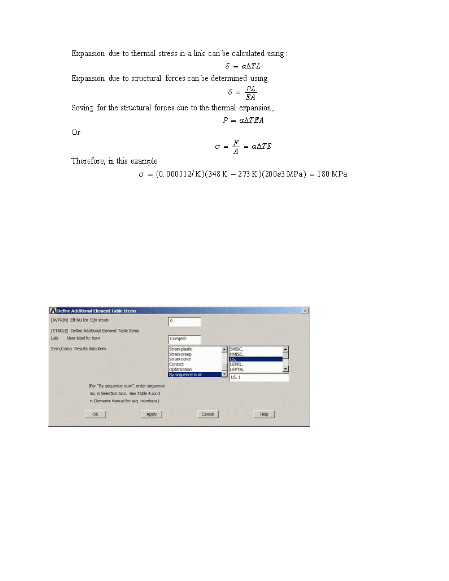
2. Get Stress Data

Since the element is only a line, the stress can't be listed in the normal way. Instead, an element
table must be created first.

General Postproc > Element Table > Define Table > Add

Fill in the window as shown below. [CompStr > By Sequence Num > LS > LS,1

ETABLE,CompStress,LS,1

3. List the Stress Data

General Postproc > Element Table > List Elem Table > COMPSTR > OK

PRETAB,CompStr

University of Alberta ANSYS Tutorials - www.mece.ualberta.ca/tutorials/ansys/AT/Coupled/Coupled.html

Copyright © 2001 University of Alberta

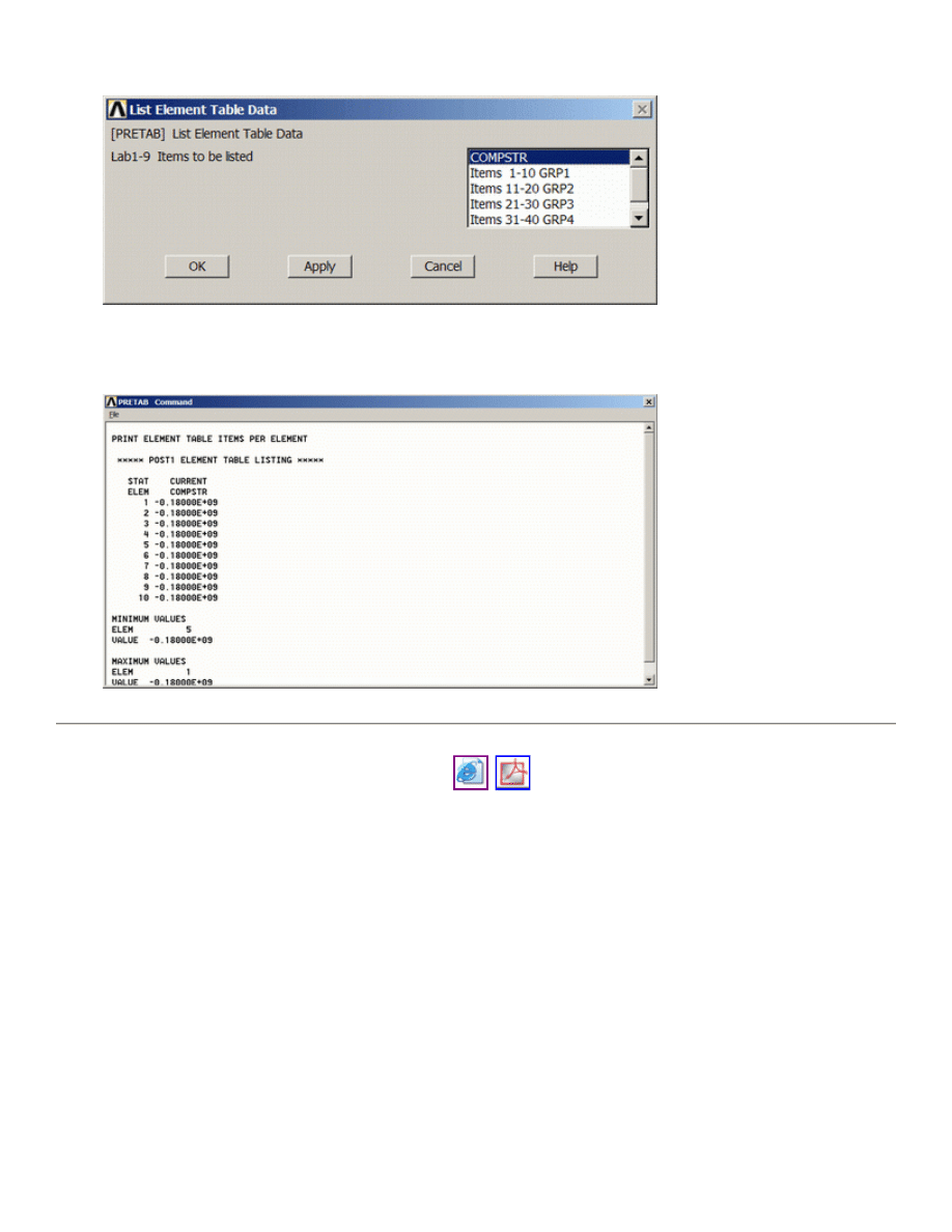
The following list should appear. Note the stress in each element: -0.180e9 Pa, or 180 MPa in
compression as expected.

Command File Mode of Solution

The above example was solved using a mixture of the Graphical User Interface (or GUI) and the command

language interface of ANSYS. This problem has also been solved using the ANSYS command language
interface that you may want to browse. Open the .HTML version, copy and paste the code into Notepad or a

similar text editor and save it to your computer. Now go to 'File > Read input from...' and select the file.

A .PDF version is also available for printing.

University of Alberta ANSYS Tutorials - www.mece.ualberta.ca/tutorials/ansys/AT/Coupled/Coupled.html

Copyright © 2001 University of Alberta