
M
ATLAB
The Language of Technical Computing
Computation
Visualization
Programming
Getting Started with MATLAB
Version 5
How to Contact The MathWorks:
508-647-7000
Phone
508-647-7001
Fax
The MathWorks, Inc.
24 Prime Park Way
Natick, MA 01760-1500
http://www.mathworks.com
Web
ftp.mathworks.com
Anonymous FTP server
comp.soft-sys.matlab
Newsgroup
support@mathworks.com
Technical support
suggest@mathworks.com
Product enhancement suggestions
bugs@mathworks.com
Bug reports
doc@mathworks.com
Documentation error reports
subscribe@mathworks.com
Subscribing user registration
service@mathworks.com
Order status, license renewals, passcodes
info@mathworks.com
Sales, pricing, and general information
Getting Started with MATLAB
COPYRIGHT 1984 - 1998 by The MathWorks, Inc.
The software described in this document is furnished under a license agreement. The software may be used
or copied only under the terms of the license agreement. No part of this manual may be photocopied or repro-
duced in any form without prior written consent from The MathWorks, Inc.
U.S. GOVERNMENT: If Licensee is acquiring the Programs on behalf of any unit or agency of the U.S.
Government, the following shall apply: (a) For units of the Department of Defense: the Government shall
have only the rights specified in the license under which the commercial computer software or commercial
software documentation was obtained, as set forth in subparagraph (a) of the Rights in Commercial
Computer Software or Commercial Software Documentation Clause at DFARS 227.7202-3, therefore the
rights set forth herein shall apply; and (b) For any other unit or agency: NOTICE: Notwithstanding any
other lease or license agreement that may pertain to, or accompany the delivery of, the computer software
and accompanying documentation, the rights of the Government regarding its use, reproduction, and disclo-
sure are as set forth in Clause 52.227-19 (c)(2) of the FAR.
MATLAB, Simulink, Stateflow, Handle Graphics, and Real-Time Workshop are registered trademarks, and
Target Language Compiler is a trademark of The MathWorks, Inc.
Other product or brand names are trademarks or registered trademarks of their respective holders.
Printing History: December 1996
First printing (for MATLAB 5)
May 1997
Second printing (for MATLAB 5.1)
September 1998
Third printing (for MATLAB 5.3)

i
Contents
Getting Started
Starting MATLAB . . . . . . . . . . . . . . . . . . . . . . . . . . . . . . . . . . . . . . . 2
Matrices and Magic Squares . . . . . . . . . . . . . . . . . . . . . . . . . . . . . 3
Entering Matrices . . . . . . . . . . . . . . . . . . . . . . . . . . . . . . . . . . . . . . 4
sum, transpose, and diag . . . . . . . . . . . . . . . . . . . . . . . . . . . . . . . . 5
Subscripts . . . . . . . . . . . . . . . . . . . . . . . . . . . . . . . . . . . . . . . . . . . . 7
The Colon Operator . . . . . . . . . . . . . . . . . . . . . . . . . . . . . . . . . . . . . 8
The magic Function . . . . . . . . . . . . . . . . . . . . . . . . . . . . . . . . . . . . . 9
Expressions . . . . . . . . . . . . . . . . . . . . . . . . . . . . . . . . . . . . . . . . . . . 11
Variables . . . . . . . . . . . . . . . . . . . . . . . . . . . . . . . . . . . . . . . . . . . . 11
Numbers . . . . . . . . . . . . . . . . . . . . . . . . . . . . . . . . . . . . . . . . . . . . . 11
Operators . . . . . . . . . . . . . . . . . . . . . . . . . . . . . . . . . . . . . . . . . . . . 12
Functions . . . . . . . . . . . . . . . . . . . . . . . . . . . . . . . . . . . . . . . . . . . . 12
Expressions . . . . . . . . . . . . . . . . . . . . . . . . . . . . . . . . . . . . . . . . . . 14
Working with Matrices . . . . . . . . . . . . . . . . . . . . . . . . . . . . . . . . . 15
Generating Matrices . . . . . . . . . . . . . . . . . . . . . . . . . . . . . . . . . . . 15
load . . . . . . . . . . . . . . . . . . . . . . . . . . . . . . . . . . . . . . . . . . . . . . . . . 16
M-Files . . . . . . . . . . . . . . . . . . . . . . . . . . . . . . . . . . . . . . . . . . . . . . 16
Concatenation . . . . . . . . . . . . . . . . . . . . . . . . . . . . . . . . . . . . . . . . 17
Deleting Rows and Columns . . . . . . . . . . . . . . . . . . . . . . . . . . . . . 17
The Command Window . . . . . . . . . . . . . . . . . . . . . . . . . . . . . . . . . 19
The format Command . . . . . . . . . . . . . . . . . . . . . . . . . . . . . . . . . . 19
Suppressing Output . . . . . . . . . . . . . . . . . . . . . . . . . . . . . . . . . . . 21
Long Command Lines . . . . . . . . . . . . . . . . . . . . . . . . . . . . . . . . . . 21
Command Line Editing . . . . . . . . . . . . . . . . . . . . . . . . . . . . . . . . . 21
Graphics . . . . . . . . . . . . . . . . . . . . . . . . . . . . . . . . . . . . . . . . . . . . . . 23
Creating a Plot . . . . . . . . . . . . . . . . . . . . . . . . . . . . . . . . . . . . . . . . 23
Figure Windows . . . . . . . . . . . . . . . . . . . . . . . . . . . . . . . . . . . . . . . 25

ii
Contents
Adding Plots to an Existing Graph . . . . . . . . . . . . . . . . . . . . . . . . 25
Subplots . . . . . . . . . . . . . . . . . . . . . . . . . . . . . . . . . . . . . . . . . . . . . 27
Imaginary and Complex Data . . . . . . . . . . . . . . . . . . . . . . . . . . . . 28
Controlling Axes . . . . . . . . . . . . . . . . . . . . . . . . . . . . . . . . . . . . . . . 29
Axis Labels and Titles . . . . . . . . . . . . . . . . . . . . . . . . . . . . . . . . . . 30
Mesh and Surface Plots . . . . . . . . . . . . . . . . . . . . . . . . . . . . . . . . . 31
Visualizing Functions of Two Variables . . . . . . . . . . . . . . . . . . . . 31
Images . . . . . . . . . . . . . . . . . . . . . . . . . . . . . . . . . . . . . . . . . . . . . . . 32
Printing Graphics . . . . . . . . . . . . . . . . . . . . . . . . . . . . . . . . . . . . . . 33
Help and Online Documentation . . . . . . . . . . . . . . . . . . . . . . . . 34
The help Command . . . . . . . . . . . . . . . . . . . . . . . . . . . . . . . . . . . . 34
The Help Window . . . . . . . . . . . . . . . . . . . . . . . . . . . . . . . . . . . . . . 35
The lookfor Command . . . . . . . . . . . . . . . . . . . . . . . . . . . . . . . . . . 36
The Help Desk . . . . . . . . . . . . . . . . . . . . . . . . . . . . . . . . . . . . . . . . 37
The doc Command . . . . . . . . . . . . . . . . . . . . . . . . . . . . . . . . . . . . . 37
Printing Online Reference Pages . . . . . . . . . . . . . . . . . . . . . . . . . 37
Link to the MathWorks . . . . . . . . . . . . . . . . . . . . . . . . . . . . . . . . . 37
The MATLAB Environment . . . . . . . . . . . . . . . . . . . . . . . . . . . . . 38
The Workspace . . . . . . . . . . . . . . . . . . . . . . . . . . . . . . . . . . . . . . . . 38
save Commands . . . . . . . . . . . . . . . . . . . . . . . . . . . . . . . . . . . . . . . 39
The Search Path . . . . . . . . . . . . . . . . . . . . . . . . . . . . . . . . . . . . . . . 39
Disk File Manipulation . . . . . . . . . . . . . . . . . . . . . . . . . . . . . . . . . 40
The diary Command . . . . . . . . . . . . . . . . . . . . . . . . . . . . . . . . . . . 40
Running External Programs . . . . . . . . . . . . . . . . . . . . . . . . . . . . . 41
More About Matrices and Arrays . . . . . . . . . . . . . . . . . . . . . . . . 42
Linear Algebra . . . . . . . . . . . . . . . . . . . . . . . . . . . . . . . . . . . . . . . . 42
Arrays . . . . . . . . . . . . . . . . . . . . . . . . . . . . . . . . . . . . . . . . . . . . . . . 45
Multivariate Data . . . . . . . . . . . . . . . . . . . . . . . . . . . . . . . . . . . . . 47
Scalar Expansion . . . . . . . . . . . . . . . . . . . . . . . . . . . . . . . . . . . . . . 48
Logical Subscripting . . . . . . . . . . . . . . . . . . . . . . . . . . . . . . . . . . . 49
The find Function . . . . . . . . . . . . . . . . . . . . . . . . . . . . . . . . . . . . . . 50

iii
Flow Control . . . . . . . . . . . . . . . . . . . . . . . . . . . . . . . . . . . . . . . . . . 52
if . . . . . . . . . . . . . . . . . . . . . . . . . . . . . . . . . . . . . . . . . . . . . . . . . . . 52
switch and case . . . . . . . . . . . . . . . . . . . . . . . . . . . . . . . . . . . . . . . 53
for . . . . . . . . . . . . . . . . . . . . . . . . . . . . . . . . . . . . . . . . . . . . . . . . . . 54
while . . . . . . . . . . . . . . . . . . . . . . . . . . . . . . . . . . . . . . . . . . . . . . . . 55
break . . . . . . . . . . . . . . . . . . . . . . . . . . . . . . . . . . . . . . . . . . . . . . . . 55
Other Data Structures . . . . . . . . . . . . . . . . . . . . . . . . . . . . . . . . . . 57
Multidimensional Arrays . . . . . . . . . . . . . . . . . . . . . . . . . . . . . . . . 57
Cell Arrays . . . . . . . . . . . . . . . . . . . . . . . . . . . . . . . . . . . . . . . . . . . 59
Characters and Text . . . . . . . . . . . . . . . . . . . . . . . . . . . . . . . . . . . 61
Structures . . . . . . . . . . . . . . . . . . . . . . . . . . . . . . . . . . . . . . . . . . . . 64
Scripts and Functions . . . . . . . . . . . . . . . . . . . . . . . . . . . . . . . . . . 67
Scripts . . . . . . . . . . . . . . . . . . . . . . . . . . . . . . . . . . . . . . . . . . . . . . . 67
Functions . . . . . . . . . . . . . . . . . . . . . . . . . . . . . . . . . . . . . . . . . . . . 69
Global Variables . . . . . . . . . . . . . . . . . . . . . . . . . . . . . . . . . . . . . . . 70
Command/Function Duality . . . . . . . . . . . . . . . . . . . . . . . . . . . . . 71
The eval Function . . . . . . . . . . . . . . . . . . . . . . . . . . . . . . . . . . . . . 71
Vectorization . . . . . . . . . . . . . . . . . . . . . . . . . . . . . . . . . . . . . . . . . 72
Preallocation . . . . . . . . . . . . . . . . . . . . . . . . . . . . . . . . . . . . . . . . . . 72
Function Functions . . . . . . . . . . . . . . . . . . . . . . . . . . . . . . . . . . . . 73
Handle Graphics . . . . . . . . . . . . . . . . . . . . . . . . . . . . . . . . . . . . . . . 76
Graphics Objects . . . . . . . . . . . . . . . . . . . . . . . . . . . . . . . . . . . . . . 76
Graphics Objects . . . . . . . . . . . . . . . . . . . . . . . . . . . . . . . . . . . . . . 76
Object Handles . . . . . . . . . . . . . . . . . . . . . . . . . . . . . . . . . . . . . . . . 77
Object Creation Functions . . . . . . . . . . . . . . . . . . . . . . . . . . . . . . . 78
Object Properties . . . . . . . . . . . . . . . . . . . . . . . . . . . . . . . . . . . . . . 78
set and get . . . . . . . . . . . . . . . . . . . . . . . . . . . . . . . . . . . . . . . . . . . 79
Graphics User Interfaces . . . . . . . . . . . . . . . . . . . . . . . . . . . . . . . . 81
Animations . . . . . . . . . . . . . . . . . . . . . . . . . . . . . . . . . . . . . . . . . . . 81
Movies . . . . . . . . . . . . . . . . . . . . . . . . . . . . . . . . . . . . . . . . . . . . . . . 83
Learning More . . . . . . . . . . . . . . . . . . . . . . . . . . . . . . . . . . . . . . . . . 85

iv
Contents

Introduction
What Is MATLAB? . . . . . . . . . . . . . . . . . . . vi

Introduction
vi
What Is MATLAB?
MATLAB is a high-performance language for technical computing. It
integrates computation, visualization, and programming in an easy-to-use
environment where problems and solutions are expressed in familiar
mathematical notation. Typical uses include:
• Math and computation
• Algorithm development
• Modeling, simulation, and prototyping
• Data analysis, exploration, and visualization
• Scientific and engineering graphics
• Application development, including Graphical User Interface building
MATLAB is an interactive system whose basic data element is an array that
does not require dimensioning. This allows you to solve many technical
computing problems, especially those with matrix and vector formulations, in
a fraction of the time it would take to write a program in a scalar noninteractive
language such as C or Fortran.
The name MATLAB stands for matrix laboratory. MATLAB was originally
written to provide easy access to matrix software developed by the LINPACK
and EISPACK projects, which together represent the state-of-the-art in
software for matrix computation.
MATLAB has evolved over a period of years with input from many users. In
university environments, it is the standard instructional tool for introductory
and advanced courses in mathematics, engineering, and science. In industry,
MATLAB is the tool of choice for high-productivity research, development, and
analysis.
MATLAB features a family of application-specific solutions called toolboxes.
Very important to most users of MATLAB, toolboxes allow you to learn and
apply specialized technology. Toolboxes are comprehensive collections of
MATLAB functions (M-files) that extend the MATLAB environment to solve
particular classes of problems. Areas in which toolboxes are available include
signal processing, control systems, neural networks, fuzzy logic, wavelets,
simulation, and many others.

vii
The MATLAB System
The MATLAB system consists of five main parts:
The MATLAB language.
This is a high-level matrix/array language with control
flow statements, functions, data structures, input/output, and object-oriented
programming features. It allows both “programming in the small” to rapidly
create quick and dirty throw-away programs, and “programming in the large”
to create complete large and complex application programs.
The MATLAB working environment.
This is the set of tools and facilities that you
work with as the MATLAB user or programmer. It includes facilities for
managing the variables in your workspace and importing and exporting data.
It also includes tools for developing, managing, debugging, and profiling
M-files, MATLAB’s applications.
Handle Graphics.
This is the MATLAB graphics system. It includes high-level
commands for two-dimensional and three-dimensional data visualization,
image processing, animation, and presentation graphics. It also includes
low-level commands that allow you to fully customize the appearance of
graphics as well as to build complete Graphical User Interfaces on your
MATLAB applications.
The MATLAB mathematical function library.
This is a vast collection of
computational algorithms ranging from elementary functions like sum, sine,
cosine, and complex arithmetic, to more sophisticated functions like matrix
inverse, matrix eigenvalues, Bessel functions, and fast Fourier transforms.
The MATLAB Application Program Interface (API).
This is a library that allows you to
write C and Fortran programs that interact with MATLAB. It include facilities
for calling routines from MATLAB (dynamic linking), calling MATLAB as a
computational engine, and for reading and writing MAT-files.
About Simulink
Simulink, a companion program to MATLAB, is an interactive system for
simulating nonlinear dynamic systems. It is a graphical mouse-driven program
that allows you to model a system by drawing a block diagram on the screen
and manipulating it dynamically. It can work with linear, nonlinear,
continuous-time, discrete-time, multivariable, and multirate systems.

Introduction
viii
Blocksets are add-ins to Simulink that provide additional libraries of blocks for
specialized applications like communications, signal processing, and power
systems.
Real-time Workshop is a program that allows you to generate C code from your
block diagrams and to run it on a variety of real-time systems.

Getting Started
. . . . . . . . . . . . . . . . . . 2
Matrices and Magic Squares . . . . . . . . . . . . . . 3
. . . . . . . . . . . . . . . . . . . . . 11
Working with Matrices . . . . . . . . . . . . . . . . 15
The Command Window . . . . . . . . . . . . . . . . 19
Graphics . . . . . . . . . . . . . . . . . . . . . . . 23
Help and Online Documentation . . . . . . . . . . . . 34
The MATLAB Environment . . . . . . . . . . . . . . 38
More About Matrices and Arrays . . . . . . . . . . . . 42
Flow Control . . . . . . . . . . . . . . . . . . . . . 52
. . . . . . . . . . . . . . . . 57
. . . . . . . . . . . . . . . . 67
Handle Graphics . . . . . . . . . . . . . . . . . . . 76
Learning More . . . . . . . . . . . . . . . . . . . . 85

Getting Started
2
Starting MATLAB
This book is intended to help you start learning MATLAB. It contains a
number of examples, so you should run MATLAB and follow along.
To run MATLAB on a PC, double-click on the MATLAB icon. To run MATLAB
on a UNIX system, type
matlab
at the operating system prompt. To quit
MATLAB at any time, type
quit
at the MATLAB prompt.
If you feel you need more assistance, type
help
at the MATLAB prompt, or pull
down on the Help menu on a PC. We will tell you more about the help and
online documentation facilities later.
Matrices and Magic Squares
3
Matrices and Magic Squares
The best way for you to get started with MATLAB is to learn how to handle
matrices. This section shows you how to do that. In MATLAB, a matrix is a
rectangular array of numbers. Special meaning is sometimes attached to
1-by-1 matrices, which are scalars, and to matrices with only one row or
column, which are vectors. MATLAB has other ways of storing both numeric
and nonnumeric data, but in the beginning, it is usually best to think of
everything as a matrix. The operations in MATLAB are designed to be as
natural as possible. Where other programming languages work with numbers
one at a time, MATLAB allows you to work with entire matrices quickly and
easily.
Getting Started
4
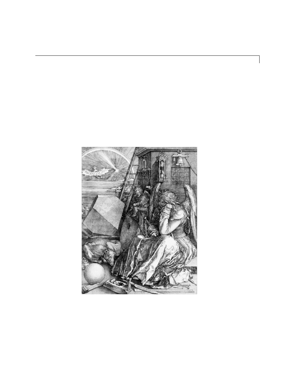
A good example matrix, used
throughout this book, appears
in the Renaissance engraving
Melancholia I by the German
artist and amateur
mathematician Albrecht Dürer.
This image is filled with
mathematical symbolism, and if
you look carefully, you will see a
matrix in the upper right
corner. This matrix is known as
a magic square and was
believed by many in Dürer’s
time to have genuinely magical
properties. It does turn out to
have some fascinating
characteristics worth exploring.
Entering Matrices
You can enter matrices into MATLAB in several different ways.
• Enter an explicit list of elements.
• Load matrices from external data files.
• Generate matrices using built-in functions.
• Create matrices with your own functions in M-files.
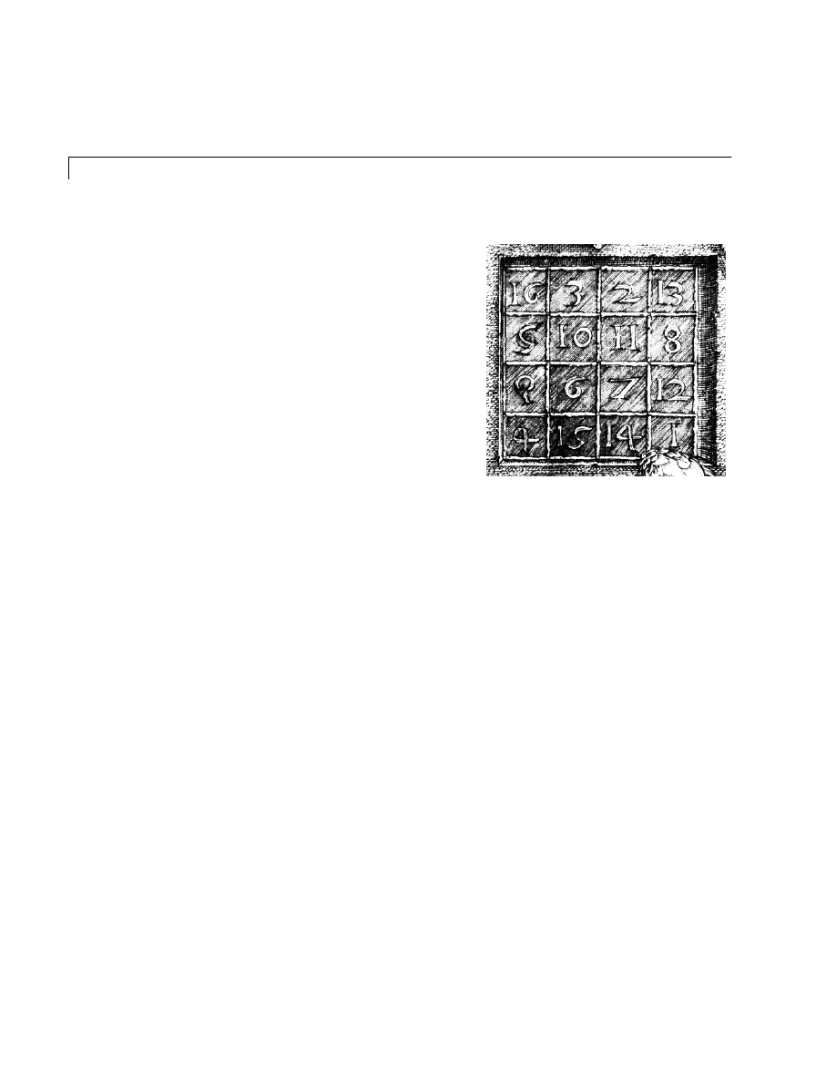
Start by entering Dürer’s matrix as a list of its elements. You have only to
follow a few basic conventions:
• Separate the elements of a row with blanks or commas.
• Use a semicolon,
;
, to indicate the end of each row.
• Surround the entire list of elements with square brackets,
[ ]
.
To enter Dürer’s matrix, simply type:
A = [16 3 2 13; 5 10 11 8; 9 6 7 12; 4 15 14 1]

Matrices and Magic Squares
5
MATLAB displays the matrix you just entered,
A =
16 3 2 13
5 10 11 8
9 6 7 12
4 15 14 1
This exactly matches the numbers in the engraving. Once you have entered the
matrix, it is automatically remembered in the MATLAB workspace. You can
refer to it simply as
A
. Now that you have
A
in the workspace, take a look at
what makes it so interesting. Why is it magic?
sum, transpose, and diag
You’re probably already aware that the special properties of a magic square
have to do with the various ways of summing its elements. If you take the sum
along any row or column, or along either of the two main diagonals, you will
always get the same number. Let’s verify that using MATLAB. The first
statement to try is
sum(A)
MATLAB replies with
ans =
34 34 34 34
When you don’t specify an output variable, MATLAB uses the variable
ans
,
short for
answer
, to store the results of a calculation. You have computed a row
vector containing the sums of the columns of
A
. Sure enough, each of the
columns has the same sum, the
magic
sum, 34.
How about the row sums? MATLAB has a preference for working with the
columns of a matrix, so the easiest way to get the row sums is to transpose the
matrix, compute the column sums of the transpose, and then transpose the
result. The transpose operation is denoted by an apostrophe or single quote,
'
.
It flips a matrix about its main diagonal and it turns a row vector into a column
vector. So
A'

Getting Started
6
produces
ans =
16 5 9 4
3 10 6 15
2 11 7 14
13 8 12 1
And
sum(A')'
produces a column vector containing the row sums
ans =
34
34
34
34
The sum of the elements on the main diagonal is easily obtained with the help
of the
diag
function, which picks off that diagonal.
diag(A)
produces
ans =
16
10
7
1
and
sum(diag(A))
produces
ans =
34

Matrices and Magic Squares
7
The other diagonal, the so-called antidiagonal, is not so important
mathematically, so MATLAB does not have a ready-made function for it. But a
function originally intended for use in graphics,
fliplr
, flips a matrix from left
to right.
sum(diag(fliplr(A)))
ans =
34
You have verified that the matrix in Dürer’s engraving is indeed a magic
square and, in the process, have sampled a few MATLAB matrix operations.
The following sections continue to use this matrix to illustrate additional
MATLAB capabilities.
Subscripts
The element in row
i
and column
j
of
A
is denoted by
A(i,j)
. For example,
A(4,2)
is the number in the fourth row and second column. For our magic
square,
A(4,2)
is
15
. So it is possible to compute the sum of the elements in the
fourth column of
A
by typing
A(1,4) + A(2,4) + A(3,4) + A(4,4)
This produces
ans =
34
but is not the most elegant way of summing a single column.
It is also possible to refer to the elements of a matrix with a single subscript,
A(k)
. This is the usual way of referencing row and column vectors. But it can
also apply to a fully two-dimensional matrix, in which case the array is
regarded as one long column vector formed from the columns of the original
matrix. So, for our magic square,
A(8)
is another way of referring to the value
15
stored in
A(4,2)
.
If you try to use the value of an element outside of the matrix, it is an error:
t = A(4,5)
Index exceeds matrix dimensions.

Getting Started
8
On the other hand, if you store a value in an element outside of the matrix, the
size increases to accommodate the newcomer:
X = A;
X(4,5) = 17
X =
16 3 2 13 0
5 10 11 8 0
9 6 7 12 0
4 15 14 1 17
The Colon Operator
The colon,
:
, is one of MATLAB’s most important operators. It occurs in several
different forms. The expression
1:10
is a row vector containing the integers from 1 to 10
1 2 3 4 5 6 7 8 9 10
To obtain nonunit spacing, specify an increment. For example
100:–7:50
is
100 93 86 79 72 65 58 51
and
0:pi/4:pi
is
0 0.7854 1.5708 2.3562 3.1416
Subscript expressions involving colons refer to portions of a matrix.
A(1:k,j)
is the first
k
elements of the
j
th column of
A
. So
sum(A(1:4,4))

Matrices and Magic Squares
9
computes the sum of the fourth column. But there is a better way. The colon by
itself refers to all the elements in a row or column of a matrix and the keyword
end
refers to the last row or column. So
sum(A(:,end))
computes the sum of the elements in the last column of
A
.
ans =
34
Why is the magic sum for a 4-by-4 square equal to 34? If the integers from 1 to
16 are sorted into four groups with equal sums, that sum must be
sum(1:16)/4
which, of course, is
ans =
34
If you have access to the
Symbolic Math Toolbox, you
can discover that the magic
sum for an n-by-n magic
square is (
n
3
+
n
)/2.
The magic Function
MATLAB actually has a built-in function that creates magic squares of almost
any size. Not surprisingly, this function is named
magic
.
B = magic(4)
B =
16 2 3 13
5 11 10 8
9 7 6 12
4 14 15 1
This matrix is almost the same as the one in the Dürer engraving and has all
the same “magic” properties; the only difference is that the two middle columns
are exchanged. To make this
B
into Dürer’s
A
, swap the two middle columns.
A = B(:,[1 3 2 4])

Getting Started
10
This says “for each of the rows of matrix
B
, reorder the elements in the order 1,
3, 2, 4.” It produces
A =
16 3 2 13
5 10 11 8
9 6 7 12
4 15 14 1
Why would Dürer go to the trouble of rearranging the columns when he could
have used MATLAB’s ordering? No doubt he wanted to include the date of the
engraving, 1514, at the bottom of his magic square.

Expressions
11
Expressions
Like most other programming languages, MATLAB provides mathematical
expressions, but unlike most programming languages, these expressions
involve entire matrices. The building blocks of expressions are
• Variables
• Numbers
• Operators
• Functions
Variables
MATLAB does not require any type declarations or dimension statements.
When MATLAB encounters a new variable name, it automatically creates the
variable and allocates the appropriate amount of storage. If the variable
already exists, MATLAB changes its contents and, if necessary, allocates new
storage. For example
num_students = 25
creates a 1-by-1 matrix named
num_students
and stores the value 25 in its
single element.
Variable names consist of a letter, followed by any number of letters, digits, or
underscores. MATLAB uses only the first 31 characters of a variable name.
MATLAB is case sensitive; it distinguishes between uppercase and lowercase
letters.
A
and
a
are not the same variable. To view the matrix assigned to any
variable, simply enter the variable name.
Numbers
MATLAB uses conventional decimal notation, with an optional decimal point
and leading plus or minus sign, for numbers. Scientific notation uses the letter
e
to specify a power-of-ten scale factor. Imaginary numbers use either
i
or
j
as
a suffix. Some examples of legal numbers are
3 –99 0.0001
9.6397238 1.60210e–20 6.02252e23
1i –3.14159j 3e5i

Getting Started
12
All numbers are stored internally using the long format specified by the IEEE
floating-point standard. Floating-point numbers have a finite precision of
roughly 16 significant decimal digits and a finite range of roughly 10
-308
to
10
+308
. (The VAX computer uses a different floating-point format, but its
precision and range are nearly the same.)
Operators
Expressions use familiar arithmetic operators and precedence rules.
Functions
MATLAB provides a large number of standard elementary mathematical
functions, including
abs
,
sqrt
,
exp
, and
sin
. Taking the square root or
logarithm of a negative number is not an error; the appropriate complex result
is produced automatically. MATLAB also provides many more advanced
mathematical functions, including Bessel and gamma functions. Most of these
functions accept complex arguments. For a list of the elementary mathematical
functions, type
help elfun
+
Addition
–
Subtraction
*
Multiplication
/
Division
\
Left division
(described in the section on Matrices and Linear
Algebra in Using MATLAB)
^
Power
'
Complex conjugate transpose
( )
Specify evaluation order

Expressions
13
For a list of more advanced mathematical and matrix functions, type
help specfun
help elmat
Some of the functions, like
sqrt
and
sin
, are built-in. They are part of the
MATLAB core so they are very efficient, but the computational details are not
readily accessible. Other functions, like
gamma
and
sinh
, are implemented in
M-files. You can see the code and even modify it if you want.
Several special functions provide values of useful constants.
Infinity is generated by dividing a nonzero value by zero, or by evaluating well
defined mathematical expressions that overflow, i.e., exceed
realmax
.
Not-a-number is generated by trying to evaluate expressions like
0/0
or
Inf–Inf
that do not have well defined mathematical values.
The function names are not reserved. It is possible to overwrite any of them
with a new variable, such as
eps = 1.e–6
and then use that value in subsequent calculations. The original function can
be restored with
clear eps
pi
3.14159265…
i
Imaginary unit,
√
-1
j
Same as
i
eps
Floating-point relative precision, 2
-52
realmin
Smallest floating-point number, 2
-1022
realmax
Largest floating-point number, (2-
ε
)2
1023
Inf
Infinity
NaN
Not-a-number

Getting Started
14
Expressions
You have already seen several examples of MATLAB expressions.
Here are a
few more examples, and the resulting values.
rho = (1+sqrt(5))/2
rho =
1.6180
a = abs(3+4i)
a =
5
z = sqrt(besselk(4/3,rho–i))
z =
0.3730+ 0.3214i
huge = exp(log(realmax))
huge =
1.7977e+308
toobig = pi*huge
toobig =
Inf

Working with Matrices
15
Working with Matrices
This section introduces you to other ways of creating matrices.
Generating Matrices
MATLAB provides four functions that generate basic matrices:
Some examples:
Z = zeros(2,4)
Z =
0 0 0 0
0 0 0 0
F = 5*ones(3,3)
F =
5 5 5
5 5 5
5 5 5
N = fix(10*rand(1,10))
N =
4 9 4 4 8 5 2 6 8 0
R = randn(4,4)
R =
1.0668 0.2944 –0.6918 –1.4410
0.0593 –1.3362 0.8580 0.5711
–0.0956 0.7143 1.2540 –0.3999
–0.8323 1.6236 –1.5937 0.6900
zeros
All zeros
ones
All ones
rand
Uniformly distributed random elements
randn
Normally distributed random elements

Getting Started
16
load
The
load
command reads binary files containing matrices generated by earlier
MATLAB sessions, or reads text files containing numeric data. The text file
should be organized as a rectangular table of numbers, separated by blanks,
with one row per line, and an equal number of elements in each row. For
example, outside of MATLAB, create a text file containing these four lines:
16.0 3.0 2.0 13.0
5.0 10.0 11.0 8.0
9.0 6.0 7.0 12.0
4.0 15.0 14.0 1.0
Store the file under the name
magik.dat
. Then the command
load magik.dat
reads the file and creates a variable,
magik
, containing our example matrix.
M-Files
You can create your own matrices using M-files, which are text files containing
MATLAB code. Just create a file containing the same statements you would
type at the MATLAB command line. Save the file under a name that ends in
.m
.
NOTE To access a text editor on a PC, choose Open or New from the File
menu or press the appropriate button on the toolbar. To access a text editor
under UNIX, use the ! symbol followed by whatever command you would
ordinarily use at your operating system prompt.
For example, create a file containing these five lines:
A = [ ...
16.0 3.0 2.0 13.0
5.0 10.0 11.0 8.0
9.0 6.0 7.0 12.0
4.0 15.0 14.0 1.0 ];

Working with Matrices
17
Store the file under the name
magik.m
. Then the statement
magik
reads the file and creates a variable,
A
, containing our example matrix.
Concatenation
Concatenation is the process of joining small matrices to make bigger ones. In
fact, you made your first matrix by concatenating its individual elements. The
pair of square brackets,
[]
, is the concatenation operator. For an example, start
with the 4-by-4 magic square,
A
, and form
B = [A A+32; A+48 A+16]
The result is an 8-by-8 matrix, obtained by joining the four submatrices.
B =
16 3 2 13 48 35 34 45
5 10 11 8 37 42 43 40
9 6 7 12 41 38 39 44
4 15 14 1 36 47 46 33
64 51 50 61 32 19 18 29
53 58 59 56 21 26 27 24
57 54 55 60 25 22 23 28
52 63 62 49 20 31 30 17
This matrix is half way to being another magic square. Its elements are a
rearrangement of the integers
1:64
. Its column sums are the correct value for
an 8-by-8 magic square.
sum(B)
ans =
260 260 260 260 260 260 260 260
But its row sums,
sum(B')'
, are not all the same. Further manipulation is
necessary to make this a valid 8-by-8 magic square.

Getting Started
18
Deleting Rows and Columns
You can delete rows and columns from a matrix using just a pair of square
brackets. Start with
X = A;
Then, to delete the second column of
X
, use
X(:,2) = []
This changes
X
to
X =
16 2 13
5 11 8
9 7 12
4 14 1
If you delete a single element from a matrix, the result isn’t a matrix anymore.
So, expressions like
X(1,2) = []
result in an error. However, using a single subscript deletes a single element,
or sequence of elements, and reshapes the remaining elements into a row
vector. So
X(2:2:10) = []
results in
X =
16 9 2 7 13 12 1

The Command Window
19
The Command Window
So far, you have been using the MATLAB command line, typing commands and
expressions, and seeing the results printed in the command window. This
section describes a few ways of altering the appearance of the command
window. If your system allows you to select the command window font or
typeface, we recommend you use a fixed width font, such as Fixedsys or
Courier, to provide proper spacing.
The format Command
The
format
command controls the numeric format of the values displayed by
MATLAB. The command affects only how numbers are displayed, not how
MATLAB computes or saves them. Here are the different formats, together
with the resulting output produced from a vector
x
with components of
different magnitudes.
x = [4/3 1.2345e–6]
format short
1.3333 0.0000
format short e
1.3333e+000 1.2345e–006
format short g
1.3333 1.2345e–006
format long
1.33333333333333 0.00000123450000
format long e
1.333333333333333e+000 1.234500000000000e–006

Getting Started
20
format long g
1.33333333333333 1.2345e–006
format bank
1.33 0.00
format rat
4/3 1/810045
format hex
3ff5555555555555 3eb4b6231abfd271
If the largest element of a matrix is larger than 10
3
or smaller than 10
-3
,
MATLAB applies a common scale factor for the short and long formats.
In addition to the
format
commands shown above
format compact
suppresses many of the blank lines that appear in the output. This lets you
view more information on a screen or window. If you want more control over
the output format, use the
sprintf
and
fprintf
functions.
Suppressing Output
If you simply type a statement and press Return or Enter, MATLAB
automatically displays the results on screen. However, if you end the line with
a semicolon, MATLAB performs the computation but does not display any
output. This is particularly useful when you generate large matrices. For
example
A = magic(100);

The Command Window
21
Long Command Lines
If a statement does not fit on one line, use three periods,
...
, followed by
Return
or Enter to indicate that the statement continues on the next line. For
example
s = 1 –1/2 + 1/3 –1/4 + 1/5 – 1/6 + 1/7 ...
– 1/8 + 1/9 – 1/10 + 1/11 – 1/12;
Blank spaces around the
=
,
+
, and
–
signs are optional, but they improve
readability.
Command Line Editing
Various arrow and control keys on your keyboard allow you to recall, edit, and
reuse commands you have typed earlier. For example, suppose you mistakenly
enter
rho = (1 + sqt(5))/2
You have misspelled
sqrt
. MATLAB responds with
Undefined function or variable 'sqt'.
Instead of retyping the entire line, simply press the
↑
key. The misspelled
command is redisplayed. Use the
←
key to move the cursor over and insert the
missing
r
. Repeated use of the
↑
key recalls earlier lines. Typing a few
characters and then the
↑
key finds a previous line that begins with those
characters.
The list of available command line editing keys is different on different
computers. Experiment to see which of the following keys is available on your
machine. (Many of these keys will be familiar to users of the EMACS editor.)
↑
ctrl-p
Recall previous line
↓
c
trl-n
Recall next line
←
ctrl-b
Move back one character
→
ctrl-f
Move forward one character
ctrl-
→
ctrl-
r
Move right one word

Getting Started
22
ctrl-
←
ctrl-
l
Move left one word
home
ctrl-a
Move to beginning of line
end
ctrl-e
Move to end of line
esc
ctrl-u
Clear line
del
ctrl-d
Delete character at cursor
backspace
ctrl-h
Delete character before cursor
c
trl-k
Delete to end of line
Graphics
23
Graphics
MATLAB has extensive facilities for displaying vectors and matrices as
graphs, as well as annotating and printing these graphs. This section describes
a few of the most important graphics functions and provides examples of some
typical applications.
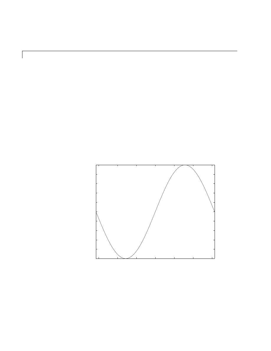
Creating a Plot
The
plot
function has different forms, depending on the input arguments. If
y
is a vector,
plot(y)
produces a piecewise linear graph of the elements of
y
versus the index of the elements of
y
. If you specify two vectors as arguments,
plot(x,y)
produces a graph of
y
versus
x
.
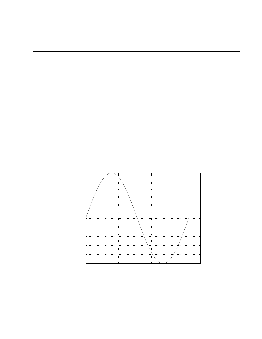
For example, to plot the value of the sine function from zero to
2π
, use
t = 0:pi/100:2*pi;
y = sin(t);
plot(t,y)
0
1
2
3
4
5
6
7
−1
−0.8
−0.6
−0.4
−0.2
0
0.2
0.4
0.6
0.8
1
Getting Started
24
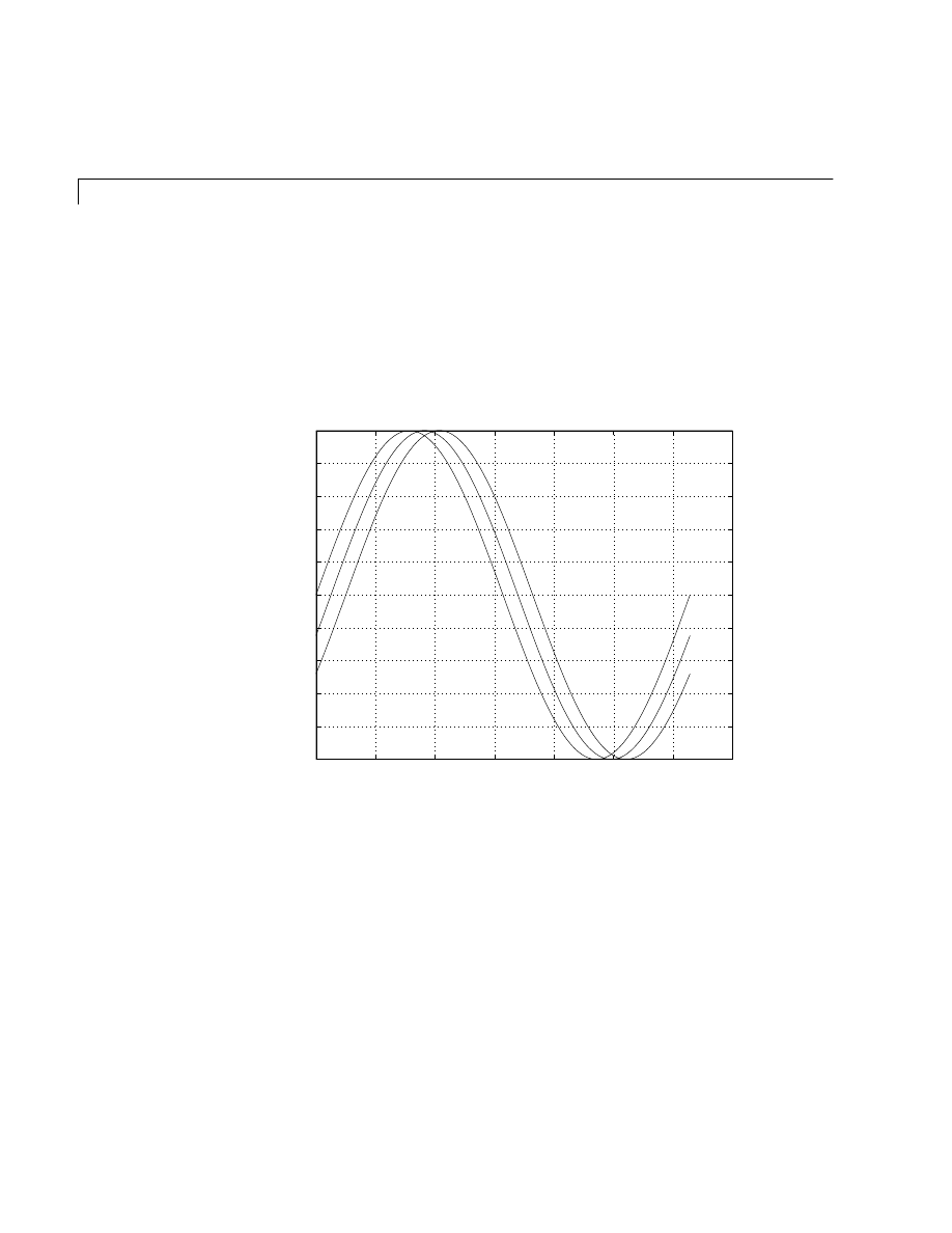
Multiple
x
-
y
pairs create multiple graphs with a single call to
plot
. MATLAB
automatically cycles through a predefined (but user settable) list of colors to
allow discrimination between each set of data. For example, these statements
plot three related functions of
t
, each curve in a separate distinguishing color:
y2 = sin(t–.25);
y3 = sin(t–.5);
plot(t,y,t,y2,t,y3)
It is possible to specify color, linestyle, and markers, such as plus signs or
circles, with:
plot(x,y,'color_style_marker')
0
1
2
3
4
5
6
7
−1
−0.8
−0.6
−0.4
−0.2
0
0.2
0.4
0.6
0.8
1

Graphics
25
color_style_marker
is a 1-, 2-, or 3-character string (delineated by single
quotation marks) constructed from a color, a linestyle, and a marker type:
• Color strings are
'c'
,
'm'
,
'y'
,
'r'
,
'g'
,
'b'
,
'w'
, and
'k'
. These correspond
to cyan, magenta, yellow, red, green, blue, white, and black.
• Linestyle strings are
'–'
for solid,
'
– –
'
for dashed,
':'
for dotted,
'–.'
for
dash-dot, and
'none'
for no line.
• The most common marker types include
'+'
,
'o'
,
'*'
, and
'x'
.
For example, the statement:
plot(x,y,'y:+')
plots a yellow dotted line and places plus sign markers at each data point. If
you specify a marker type but not a linestyle, MATLAB draws only the marker.
Figure Windows
The
plot
function automatically opens a new figure window if there are no
figure windows already on the screen. If a figure window exists,
plot
uses that
window by default. To open a new figure window and make it the current
figure, type
figure
To make an existing figure window the current figure, type
figure(n)
where
n
is the number in the figure title bar. The results of subsequent
graphics commands are displayed in this window.
Adding Plots to an Existing Graph
The
hold
command allows you to add plots to an existing graph. When you type
hold on
MATLAB does not remove the existing graph; it adds the new data to the
current graph, rescaling if necessary. For example, these statements first
Getting Started
26
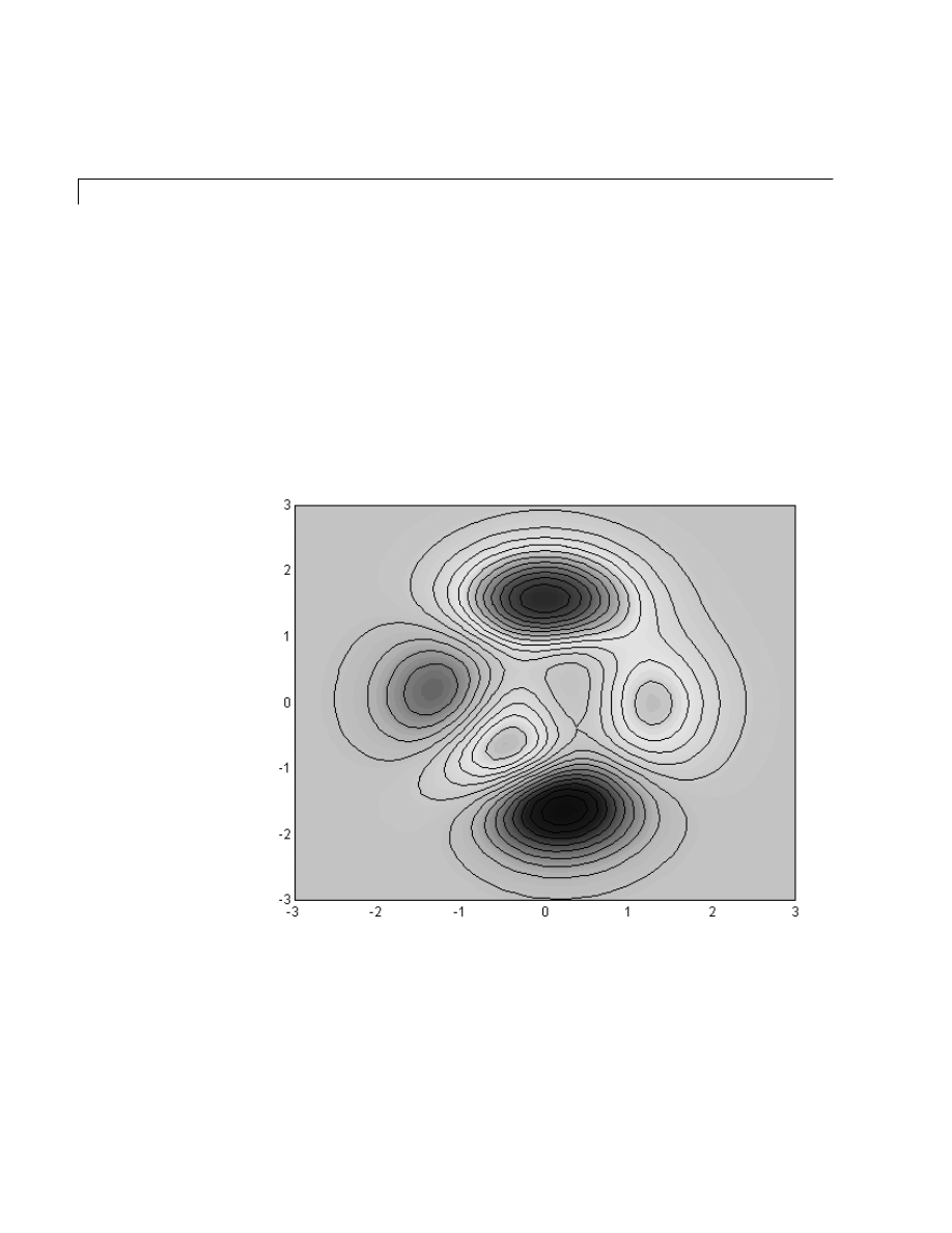
create a contour plot of the
peaks
function, then superimpose a pseudocolor plot
of the same function:
[x,y,z] = peaks;
contour(x,y,z,20,'k')
hold on
pcolor(x,y,z)
shading interp
The
hold on
command causes the
pcolor
plot to be combined with the
contour
plot in one figure.
Graphics
27
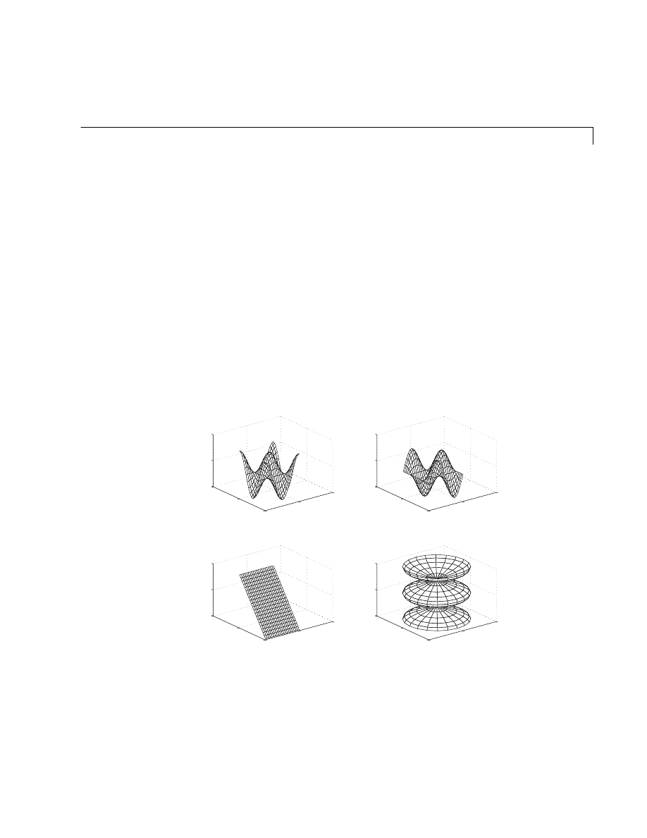
Subplots
The
subplot
function allows you to display multiple plots in the same window
or print them on the same piece of paper. Typing
subplot(m,n,p)
breaks the figure window into an
m
-by-
n
matrix of small subplots and selects
the
p
th subplot for the current plot. The plots are numbered along first the top
row of the figure window, then the second row, and so on. For example, to plot
data in four different subregions of the figure window,
t = 0:pi/10:2*pi;
[X,Y,Z] = cylinder(4*cos(t));
subplot(2,2,1)
mesh(X)
subplot(2,2,2); mesh(Y)
subplot(2,2,3); mesh(Z)
subplot(2,2,4); mesh(X,Y,Z)
0
20
40
0
20
40
−5
0
5
0
20
40
0
20
40
−5
0
5
0
20
40
0
20
40
0
0.5
1
−5
0
5
−5
0
5
0
0.5
1
Getting Started
28
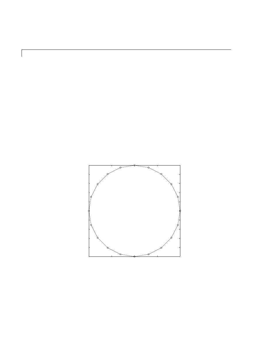
Imaginary and Complex Data
When the arguments to
plot
are complex, the imaginary part is ignored except
when
plot
is given a single complex argument. For this special case, the
command is a shortcut for a plot of the real part versus the imaginary part.
Therefore,
plot(Z)
where
Z
is a complex vector or matrix, is equivalent to
plot(real(Z),imag(Z))
For example
t = 0:pi/10:2*pi;
plot(exp(i*t),'–o')
draws a 20-sided polygon with little circles at the vertices.
−1
−0.5
0
0.5
1
−1
−0.8
−0.6
−0.4
−0.2
0
0.2
0.4
0.6
0.8
1

Graphics
29
Controlling Axes
The
axis
function has a number of options for customizing the scaling,
orientation, and aspect ratio of plots.
Ordinarily, MATLAB finds the maxima and minima of the data and chooses an
appropriate plot box and axes labeling. The
axis
function overrides the default
by setting custom axis limits,
axis([xmin xmax ymin ymax])
axis
also accepts a number of keywords for axes control. For example
axis square
makes the entire x-axes and y-axes the same length and
axis equal
makes the individual tick mark increments on the x- and y-axes the same
length. So
plot(exp(i*t))
followed by either
axis square
or
axis equal
turns the oval into a proper
circle.
axis auto
returns the axis scaling to its default, automatic mode.
axis on
turns on axis labeling and tick marks.
axis off
turns off axis labeling and tick marks.
The statement
grid off
turns the grid lines off and
grid on
turns them back on again.
Getting Started
30
Axis Labels and Titles
The
xlabel
,
ylabel
, and
zlabel
functions add x-,
y
-, and z-axis labels. The
title
function adds a title at the top of the figure and the
text
function inserts
text anywhere in the figure. A subset of Tex notation produces Greek letters,
mathematical symbols, and alternate fonts. The following example uses
\leq
for ð,
\pi
for ¼, and
\it
for italic font.
t = –pi:pi/100:pi;
y = sin(t);
plot(t,y)
axis([–pi pi –1 1])
xlabel('–\pi \leq {\itt} \leq \pi')
ylabel('sin(t)')
title('Graph of the sine function')
text(1,–1/3,'\it{Note the odd symmetry.}')
−3
−2
−1
0
1
2
3
−1
−0.8
−0.6
−0.4
−0.2
0
0.2
0.4
0.6
0.8
1
−
π
≤
t
≤
π
sin(t)
Graph of the sine function
Note the odd symmetry.

Graphics
31
Mesh and Surface Plots
MATLAB defines a surface by the z-coordinates of points above a grid in the x-y
plane, using straight lines to connect adjacent points. The functions
mesh
and
surf
display surfaces in three dimensions.
mesh
produces wireframe surfaces
that color only the lines connecting the defining points.
surf
displays both the
connecting lines and the faces of the surface in color.
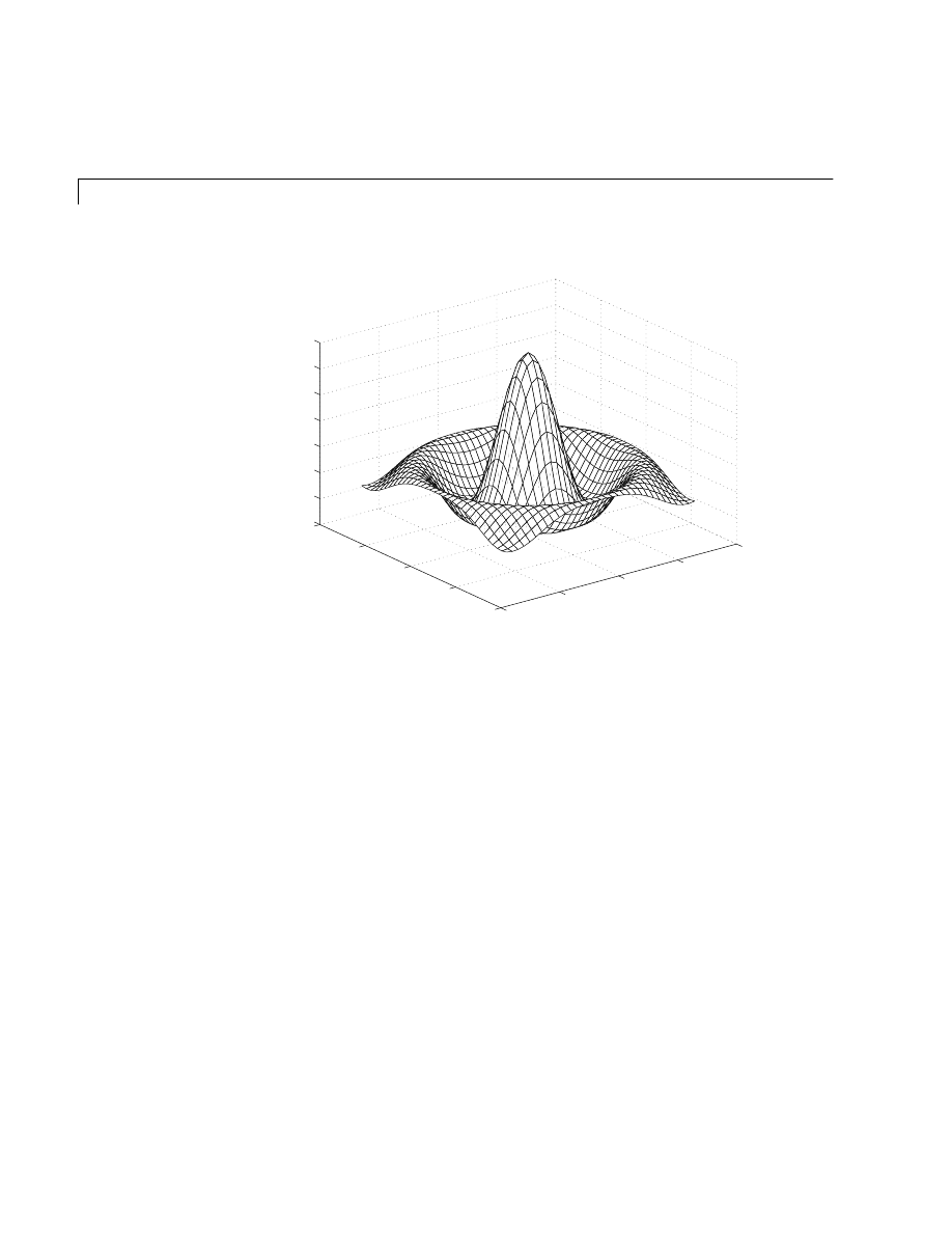
Visualizing Functions of Two Variables
To display a function of two variables, z = f (x,y), generate
X
and
Y
matrices
consisting of repeated rows and columns, respectively, over the domain of the
function. Then use these matrices to evaluate and graph the function. The
meshgrid
function transforms the domain specified by a single vector or two
vectors
x
and
y
into matrices
X
and
Y
for use in evaluating functions of two
variables. The rows of
X
are copies of the vector
x
and the columns of
Y
are
copies of the vector
y
.
To evaluate the two-dimensional sinc function, sin(r)/r, between x and y
directions:
[X,Y] = meshgrid(–8:.5:8);
R = sqrt(X.^2 + Y.^2) + eps;
Z = sin(R)./R;
mesh(X,Y,Z)
Getting Started
32
In this example,
R
is the distance from origin, which is at the center of the
matrix. Adding
eps
avoids the indeterminate 0/0 at the origin.
Images
Two-dimensional arrays can be displayed as images, where the array elements
determine brightness or color of the images. For example,
load durer
whos
shows that file
durer.mat
in the demo directory contains a 648-by-509 matrix,
X
, and a 128-by-3 matrix,
map
. The elements of
X
are integers between 1 and
128, which serve as indices into the color map,
map
. Then
image(X)
colormap(map)
axis image
−10
−5
0
5
10
−10
−5
0
5
10
−0.4
−0.2
0
0.2
0.4
0.6
0.8
1

Graphics
33
reproduces Dürer’s etching shown at the beginning of this book. A high
resolution scan of the magic square in the upper right corner is available in
another file. Type
load detail
and then use the uparrow key on your keyboard to reexecute the
image
,
colormap
, and
axis
commands. The statement
colormap(hot)
adds some twentieth century colorization to the sixteenth century etching.
Printing Graphics
The Print option on the File menu and the
command both print
MATLAB figures. The Print menu brings up a dialog box that lets you select
common standard printing options. The
command provides more
flexibility in the type of output and allows you to control printing from M-files.
The result can be sent directly to your default printer or stored in a specified
file. A wide variety of output formats, including PostScript, is available.
For example, this statement saves the contents of the current figure window as
color Encapsulated Level 2 PostScript in the file called
magicsquare.eps
:
print –depsc2 magicsquare.eps
It’s important to know the capabilities of your printer before using the
command. For example, Level 2 Postscript files are generally smaller and
render more quickly when printing than Level 1 Postscript. However, not all
PostScript printers support Level 2, so you need to know what your output
device can handle. MATLAB produces graduated output for surfaces and
patches, even for black and white output devices. However, lines and text are
printed in black or white.

Getting Started
34
Help and Online Documentation
There are several different ways to access online information about MATLAB
functions.
• The
help
command
• The help window
• The MATLAB Help Desk
• Online reference pages
• Link to The MathWorks, Inc.
The help Command
The
help
command is the most basic way to determine the syntax and behavior
of a particular function. Information is displayed directly in the command
window. For example
help magic
prints
MAGIC Magic square.
MAGIC(N) is an N–by–N matrix constructed from
the integers 1 through N^2 with equal row,
column, and diagonal sums.
Produces valid magic squares for N = 1,3,4,5....
NOTE
MATLAB online
help
entries use uppercase characters for the
function and variable names to make them stand out from the rest of the text.
When typing function names, however, always use the corresponding
lowercase characters because MATLAB is case sensitive and all function
names are actually in lowercase.

Help and Online Documentation
35
All the MATLAB functions are organized into logical groups, and MATLAB’s
directory structure is based on this grouping. For example, all the linear
algebra functions reside in the
matfun
directory. To list the names of all the
functions in that directory, with a brief description of each:
help matfun
Matrix functions – numerical linear algebra.
Matrix analysis.
norm – Matrix or vector norm.
normest – Estimate the matrix 2–norm
...
The command
help
by itself lists all the directories, with a description of the function category each
represents:
matlab/general
matlab/ops
...
The Help Window
The MATLAB help window is available on PCs by selecting the Help Window
option under the Help menu, or by clicking the question mark on the menu bar.
It is also available on all computers by typing
helpwin
To use the help window on a particular topic, type
helpwin topic
The help window gives you access to the same information as the
help
command, but the window interface provides convenient links to other topics.

Getting Started
36
The lookfor Command
The
lookfor
command allows you to search for functions based on a keyword.
It searches through the first line of
help
text, which is known as the H1 line,
for each MATLAB function, and returns the H1 lines containing a specified
keyword. For example, MATLAB does not have a function named
inverse
. So
the response from
help inverse
is
inverse.m not found.
But
lookfor inverse
finds over a dozen matches. Depending on which toolboxes you have installed,
you will find entries like
INVHILB Inverse Hilbert matrix.
ACOSH Inverse hyperbolic cosine.
ERFINV Inverse of the error function.
INV Matrix inverse.
PINV Pseudoinverse.
IFFT Inverse discrete Fourier transform.
IFFT2 Two–dimensional inverse discrete Fourier transform.
ICCEPS Inverse complex cepstrum.
IDCT Inverse discrete cosine transform.
Adding
–all
to the
lookfor
command, as in
lookfor –all
searches the entire help entry, not just the H1 line.

Help and Online Documentation
37
The Help Desk
The MATLAB Help Desk provides access to a wide range of help and reference
information stored on a disk or CD-ROM in your local system. Many of the
underlying documents use HyperText Markup Language (HTML) and are
accessed with an Internet Web browser such as Netscape or Microsoft
Explorer. The Help Desk process can be started on PCs by selecting the Help
Desk
option under the Help menu, or, on all computers, by typing
helpdesk
All of MATLAB’s operators and functions have online reference pages in HTML
format, which you can reach from the Help Desk. These pages provide more
details and examples than the basic
help
entries. HTML versions of other
documents, including this manual, are also available. A search engine, running
on your own machine, can query all the online reference material.
The doc Command
If you know the name of a specific function, you can view its reference page
directly. For example, to get the reference page for the eval function, type
doc eval
The
doc
command starts your Web browser, if it is not already running.
Printing Online Reference Pages
Versions of the online reference pages, as well as the rest of the MATLAB
documentation set, are also available in Portable Document Format (PDF)
through the Help Desk. These pages are processed by Adobe’s Acrobat reader.
They reproduce the look and feel of the printed page, complete with fonts,
graphics, formatting, and images. This is the best way to get printed copies of
reference material.
Link to the MathWorks
If your computer is connected to the Internet, the Help Desk provides a
connection to The MathWorks, the home of MATLAB. You can use electronic
mail to ask questions, make suggestions, and report possible bugs. You can also
use the Solution Search Engine at The MathWorks Web site to query an
up-to-date data base of technical support information.

Getting Started
38
The MATLAB Environment
The MATLAB environment includes both the set of variables built up during a
MATLAB session and the set of disk files containing programs and data that
persist between sessions.
The Workspace
The workspace is the area of memory accessible from the MATLAB command
line. Two commands,
who
and
whos,
show the current contents of the
workspace. The
who
command gives a short list, while
whos
also gives size and
storage information.
Here is the output produced by
whos
on a workspace containing results from
some of the examples in this book. It shows several different MATLAB data
structures. As an exercise, you might see if you can match each of the variables
with the code segment in this book that generates it.
whos
Name Size Bytes Class
A 4x4 128 double array
D 5x3 120 double array
M 10x1 3816 cell array
S 1x3 442 struct array
h 1x11 22 char array
n 1x1 8 double array
s 1x5 10 char array
v 2x5 20 char array
Grand total is 471 elements using 4566 bytes.
To delete all the existing variables from the workspace, enter
clear

The MATLAB Environment
39
save Commands
The
save
commands preserve the contents of the workspace in a MAT-file that
can be read with the
load
command in a later MATLAB session. For example
save August17th
saves the entire workspace contents in the file
August17th.mat
. If desired, you
can save only certain variables by specifying the variable names after the
filename.
Ordinarily, the variables are saved in a binary format that can be read quickly
(and accurately) by MATLAB. If you want to access these files outside of
MATLAB, you may want to specify an alternative format.
When you save workspace contents in text format, you should save only one
variable at a time. If you save more than one variable, MATLAB will create the
text file, but you will be unable to load it easily back into MATLAB.
The Search Path
MATLAB uses a search path, an ordered list of directories, to determine how
to execute the functions you call. When you call a standard function, MATLAB
executes the first M-file function on the path that has the specified name. You
can override this behavior using special private directories and subfunctions.
The command
path
shows the search path on any platform. On PCs, choose Set Path from the File
menu to view or modify the path.
–ascii
Use 8-digit text format.
–ascii –double
Use 16-digit text format.
–ascii –double –tabs
Delimit array elements with tabs.
–v4
Create a file for MATLAB version 4.
–append
Append data to an existing MAT-file.

Getting Started
40
Disk File Manipulation
The commands
dir
,
type
,
delete
, and
cd
implement a set of generic operating
system commands for manipulating files. This table indicates how these
commands map to other operating systems.
For most of these commands, you can use pathnames, wildcards, and drive
designators in the usual way.
The diary Command
The
diary
command creates a diary of your MATLAB session in a disk file. You
can view and edit the resulting text file using any word processor. To create a
file called
diary
that contains all the commands you enter, as well as
MATLAB’s printed output (but not the graphics output), enter
diary
To save the MATLAB session in a file with a particular name, use
diary filename
To stop recording the session, use
diary off
MATLAB
MS-DOS
UNIX
VAX/VMS
dir
dir
ls
dir
type
type
cat
type
delete
del or erase
rm
delete
cd
chdir
cd
set default

The MATLAB Environment
41
Running External Programs
The exclamation point character ! is a shell escape and indicates that the rest
of the input line is a command to the operating system. This is quite useful for
invoking utilities or running other programs without quitting MATLAB. On
VMS, for example,
!edt magik.m
invokes an editor called
edt
for a file named
magik.m
. When you quit the
external program, the operating system returns control to MATLAB.

Getting Started
42
More About Matrices and Arrays
This sections shows you more about working with matrices and arrays,
focusing on
• Linear Algebra
• Arrays
• Multivariate Data
Linear Algebra
Informally, the terms matrix and array are often used interchangeably. More
precisely, a matrix is a two-dimensional numeric array that represents a linear
transformation. The mathematical operations defined on matrices are the
subject of linear algebra.
Dürer’s magic square
A =
16 3 2 13
5 10 11 8
9 6 7 12
4 15 14 1
provides several examples that give a taste of MATLAB matrix operations.
You’ve already seen the matrix transpose,
A
'. Adding a matrix to its transpose
produces a symmetric matrix.
A + A'
ans =
32 8 11 17
8 20 17 23
11 17 14 26
17 23 26 2

More About Matrices and Arrays
43
The multiplication symbol,
*
, denotes the matrix multiplication involving inner
products between rows and columns. Multiplying a matrix by its transpose also
produces a symmetric matrix.
A'*A
ans =
378 212 206 360
212 370 368 206
206 368 370 212
360 206 212 378
The determinant of this particular matrix happens to be zero, indicating that
the matrix is singular.
d = det(A)
d =
0
The reduced row echelon form of
A
is not the identity.
R = rref(A)
R =
1 0 0 1
0 1 0 –3
0 0 1 3
0 0 0 0
Since the matrix is singular, it does not have an inverse. If you try to compute
the inverse with
X = inv(A)
you will get a warning message
Warning: Matrix is close to singular or badly scaled.
Results may be inaccurate. RCOND = 1.175530e–017.
Roundoff error has prevented the matrix inversion algorithm from detecting
exact singularity. But the value of
rcond
, which stands for reciprocal condition
estimate, is on the order of
eps
, the floating-point relative precision, so the
computed inverse is unlikely to be of much use.

Getting Started
44
The eigenvalues of the magic square are interesting.
e = eig(A)
e =
34.0000
8.0000
0.0000
–8.0000
One of the eigenvalues is zero, which is another consequence of singularity.
The largest eigenvalue is 34, the magic sum. That’s because the vector of all
ones is an eigenvector.
v = ones(4,1)
v =
1
1
1
1
A*v
ans =
34
34
34
34
When a magic square is scaled by its magic sum,
P = A/34
the result is a doubly stochastic matrix whose row and column sums are all one.
P =
0.4706 0.0882 0.0588 0.3824
0.1471 0.2941 0.3235 0.2353
0.2647 0.1765 0.2059 0.3529
0.1176 0.4412 0.4118 0.0294

More About Matrices and Arrays
45
Such matrices represent the transition probabilities in a Markov process.
Repeated powers of the matrix represent repeated steps of the process. For our
example, the fifth power
P^5
is
0.2507 0.2495 0.2494 0.2504
0.2497 0.2501 0.2502 0.2500
0.2500 0.2498 0.2499 0.2503
0.2496 0.2506 0.2505 0.2493
This shows that as k approaches infinity, all the elements in the kth power, P
k
,
approach
1
/
4
.
Finally, the coefficients in the characteristic polynomial
poly(A)
are
1 –34 –64 2176 0
This indicates that the characteristic polynomial
det( A -
λ
I )
is
λ
4
- 34
λ
3
- 64
λ
2
+ 2176
λ
The constant term is zero, because the matrix is singular, and the coefficient of
the cubic term is -34, because the matrix is magic!
Arrays
When they are taken away from the world of linear algebra, matrices become
two dimensional numeric arrays. Arithmetic operations on arrays are done
element-by-element. This means that addition and subtraction are the same
for arrays and matrices, but that multiplicative operations are different.
MATLAB uses a dot, or decimal point, as part of the notation for multiplicative
array operations.

Getting Started
46
The list of operators includes:
If the Dürer magic square is multiplied by itself with array multiplication
A.*A
the result is an array containing the squares of the integers from 1 to 16, in an
unusual order.
ans =
256 9 4 169
25 100 121 64
81 36 49 144
16 225 196 1
Array operations are useful for building tables. Suppose
n
is the column vector
n = (0:9)';
Then
pows = [n n.^2 2.^n]
+
Addition
-
Subtraction
.*
Element-by-element multiplication
./
Element-by-element division
.\
Element-by-element left division
.^
Element-by-element power
.'
Unconjugated array transpose

More About Matrices and Arrays
47
builds a table of squares and powers of two.
pows =
0 0 1
1 1 2
2 4 4
3 9 8
4 16 16
5 25 32
6 36 64
7 49 128
8 64 256
9 81 512
The elementary math functions operate on arrays element by element. So
format short g
x = (1:0.1:2)';
logs = [x log10(x)]
builds a table of logarithms.
logs =
1.0 0
1.1 0.04139
1.2 0.07918
1.3 0.11394
1.4 0.14613
1.5 0.17609
1.6 0.20412
1.7 0.23045
1.8 0.25527
1.9 0.27875
2.0 0.30103
Multivariate Data
MATLAB uses column-oriented analysis for multivariate statistical data. Each
column in a data set represents a variable and each row an observation. The
(i,j)
th element is the
i
th observation of the
j
th variable.

Getting Started
48
As an example, consider a data set with three variables:
• Heart rate
• Weight
• Hours of exercise per week
For five observations, the resulting array might look like:
D =
72 134 3.2
81 201 3.5
69 156 7.1
82 148 2.4
75 170 1.2
The first row contains the heart rate, weight, and exercise hours for patient 1,
the second row contains the data for patient 2, and so on. Now you can apply
many of MATLAB’s data analysis functions to this data set. For example, to
obtain the mean and standard deviation of each column:
mu = mean(D), sigma = std(D)
mu =
75.8 161.8
3.48
sigma =
5.6303
25.499 2.2107
For a list of the data analysis functions available in MATLAB, type
help datafun
If you have access to the Statistics Toolbox, type
help stats
Scalar Expansion
Matrices and scalars can be combined in several different ways. For example,
a scalar is subtracted from a matrix by subtracting it from each element. The
average value of the elements in our magic square is 8.5, so
B = A – 8.5

More About Matrices and Arrays
49
forms a matrix whose column sums are zero.
B =
7.5 –5.5 –6.5 4.5
–3.5 1.5 2.5 –0.5
0.5 –2.5 –1.5 3.5
–4.5 6.5 5.5 –7.5
sum(B)
ans =
0 0 0 0
With scalar expansion, MATLAB assigns a specified scalar to all indices in a
range. For example:
B(1:2,2:3) = 0
zeros out a portion of
B
B =
7.5 0 0 4.5
–3.5 0 0 –0.5
0.5 –2.5 –1.5 3.5
–4.5 6.5 5.5 –7.5
Logical Subscripting
The logical vectors created from logical and relational operations can be used
to reference subarrays. Suppose
X
is an ordinary matrix and
L
is a matrix of the
same size that is the result of some logical operation. Then
X(L)
specifies the
elements of
X
where the elements of
L
are nonzero.
This kind of subscripting can be done in one step by specifying the logical
operation as the subscripting expression. Suppose you have the following set of
data.
x =
2.1 1.7 1.6 1.5 NaN 1.9 1.8 1.5 5.1 1.8 1.4 2.2 1.6 1.8
The
NaN
is a marker for a missing observation, such as a failure to respond to
an item on a questionnaire. To remove the missing data with logical indexing,

Getting Started
50
use
finite(x)
, which is true for all finite numerical values and false for
NaN
and
Inf
.
x = x(finite(x))
x =
2.1 1.7 1.6 1.5 1.9 1.8 1.5 5.1 1.8 1.4 2.2 1.6 1.8
Now there is one observation,
5.1
, which seems to be very different from the
others. It is an outlier. The following statement removes outliers, in this case
those elements more than three standard deviations from the mean.
x = x(abs(x–mean(x)) <= 3*std(x))
x =
2.1 1.7 1.6 1.5 1.9 1.8 1.5 1.8 1.4 2.2 1.6 1.8
For another example, highlight the location of the prime numbers in Dürer’s
magic square by using logical indexing and scalar expansion to set the
nonprimes to 0.
A(~isprime(A)) = 0
A =
0 3 2 13
5 0 11 0
0 0 7 0
0 0 0 0
The find Function
The
find
function determines the indices of array elements that meet a given
logical condition. In its simplest form,
find
returns a column vector of indices.
Transpose that vector to obtain a row vector of indices. For example
k = find(isprime(A))'
picks out the locations, using one-dimensional indexing, of the primes in the
magic square.
k =
2 5 9 10 11 13

More About Matrices and Arrays
51
Display those primes, as a row vector in the order determined by
k
, with
A(k)
ans =
5 3 2 11 7 13
When you use
k
as a left-hand-side index in an assignment statement, the
matrix structure is preserved.
A(k) = NaN
A =
16 NaN NaN NaN
NaN 10 NaN 8
9 6 NaN 12
4 15 14 1

Getting Started
52
Flow Control
MATLAB has five flow control constructs:
• if statements
• switch statements
• for loops
• while loops
• break statements
if
The
if
statement evaluates a logical expression and executes a group of
statements when the expression is true. The optional
elseif
and
else
keywords provide for the execution of alternate groups of statements. An
end
keyword, which matches the
if
, terminates the last group of statements. The
groups of statements are delineated by the four keywords – no braces or
brackets are involved.
MATLAB’s algorithm for generating a magic square of order n involves three
different cases: when n is odd, when n is even but not divisible by 4, or when n
is divisible by 4. This is described by
if rem(n,2) ~= 0
M = odd_magic(n)
elseif rem(n,4) ~= 0
M = single_even_magic(n)
else
M = double_even_magic(n)
end
In this example, the three cases are mutually exclusive, but if they weren’t, the
first true condition would be executed.
It is important to understand how relational operators and
if
statements work
with matrices. When you want to check for equality between two variables, you
might use
if A == B, ...

Flow Control
53
This is legal MATLAB code, and does what you expect when
A
and
B
are scalars.
But when
A
and
B
are matrices,
A == B
does not test if they are equal, it tests
where they are equal; the result is another matrix of 0’s and 1’s showing
element-by-element equality. In fact, if
A
and
B
are not the same size, then
A == B
is an error.
The proper way to check for equality between two variables is to use the
isequal
function,
if isequal(A,B), ...
Here is another example to emphasize this point. If
A
and
B
are scalars, the
following program will never reach the unexpected situation. But for most
pairs of matrices, including our magic squares with interchanged columns,
none of the matrix conditions
A > B
,
A < B
or
A == B
is true for all elements
and so the
else
clause is executed.
if A > B
'greater'
elseif A < B
'less'
elseif A == B
'equal'
else
error('Unexpected situation')
end
Several functions are helpful for reducing the results of matrix comparisons to
scalar conditions for use with
if
, including
isequal
isempty
all
any
switch and case
The
switch
statement executes groups of statements based on the value of a
variable or expression. The keywords
case
and
otherwise
delineate the
groups. Only the first matching case is executed. There must always be an
end
to match the
switch
.

Getting Started
54
The logic of the magic squares algorithm can also be described by
switch (rem(n,4)==0) + (rem(n,2)==0)
case 0
M = odd_magic(n)
case 1
M = single_even_magic(n)
case 2
M = double_even_magic(n)
otherwise
error(’This is impossible’)
end
Note for C Programmers Unlike the C language
switch
statement,
MATLAB’s
switch
does not fall through. If the first case statement is true, the
other case statements do not execute. So, break statements are not required.
for
The
for
loop repeats a group of statements a fixed, predetermined number of
times. A matching
end
delineates the statements.
for n = 3:32
r(n) = rank(magic(n));
end
r
The semicolon terminating the inner statement suppresses repeated printing,
and the
r
after the loop displays the final result.
It is a good idea to indent the loops for readability, especially when they are
nested.
for i = 1:m
for j = 1:n
H(i,j) = 1/(i+j);
end
end

Flow Control
55
while
The
while
loop repeats a group of statements an indefinite number of times
under control of a logical condition. A matching
end
delineates the statements.
Here is a complete program, illustrating
while
,
if
,
else
, and
end
, that uses
interval bisection to find a zero of a polynomial.
a = 0; fa = –Inf;
b = 3; fb = Inf;
while b–a > eps*b
x = (a+b)/2;
fx = x^3–2*x–5;
if sign(fx) == sign(fa)
a = x; fa = fx;
else
b = x; fb = fx;
end
end
x
The result is a root of the polynomial x
3
- 2x - 5, namely
x =
2.09455148154233
The cautions involving matrix comparisons that are discussed in the section on
the
if
statement also apply to the
while
statement.
break
The
break
statement lets you exit early from a
for
or
while
loop. In nested
loops,
break
exits from the innermost loop only.

Getting Started
56
Here is an improvement on the example from the previous section. Why is this
use of
break
a good idea?
a = 0; fa = –Inf;
b = 3; fb = Inf;
while b–a > eps*b
x = (a+b)/2;
fx = x^3–2*x–5;
if fx == 0
break
elseif sign(fx) == sign(fa)
a = x; fa = fx;
else
b = x; fb = fx;
end
end
x

Other Data Structures
57
Other Data Structures
This section introduces you to some other data structures in MATLAB,
including:
• Multidimensional arrays
• Cell arrays
• Characters and text
• Structures
Multidimensional Arrays
Multidimensional arrays in MATLAB are arrays with more than two
subscripts. They can be created by calling
zeros
,
ones
,
rand
, or
randn
with
more than two arguments. For example
R = randn(3,4,5);
creates a 3-by-4-by-5 array with a total of 3x4x5 = 60 normally distributed
random elements.
A three-dimensional array might represent three-dimensional physical data,
say the temperature in a room, sampled on a rectangular grid. Or, it might
represent a sequence of matrices, A
(k)
, or samples of a time-dependent matrix,
A(t). In these latter cases, the (i, j)th element of the kth matrix, or the t
k
th
matrix, is denoted by
A(i,j,k)
.
MATLAB’s and Dürer’s versions of the magic square of order 4 differ by an
interchange of two columns. Many different magic squares can be generated by
interchanging columns. The statement
p = perms(1:4);
generates the 4! = 24 permutations of
1:4
. The
k
th permutation is the row
vector,
p(k,:)
. Then
A = magic(4);
M = zeros(4,4,24);
for k = 1:24
M(:,:,k) = A(:,p(k,:));
end
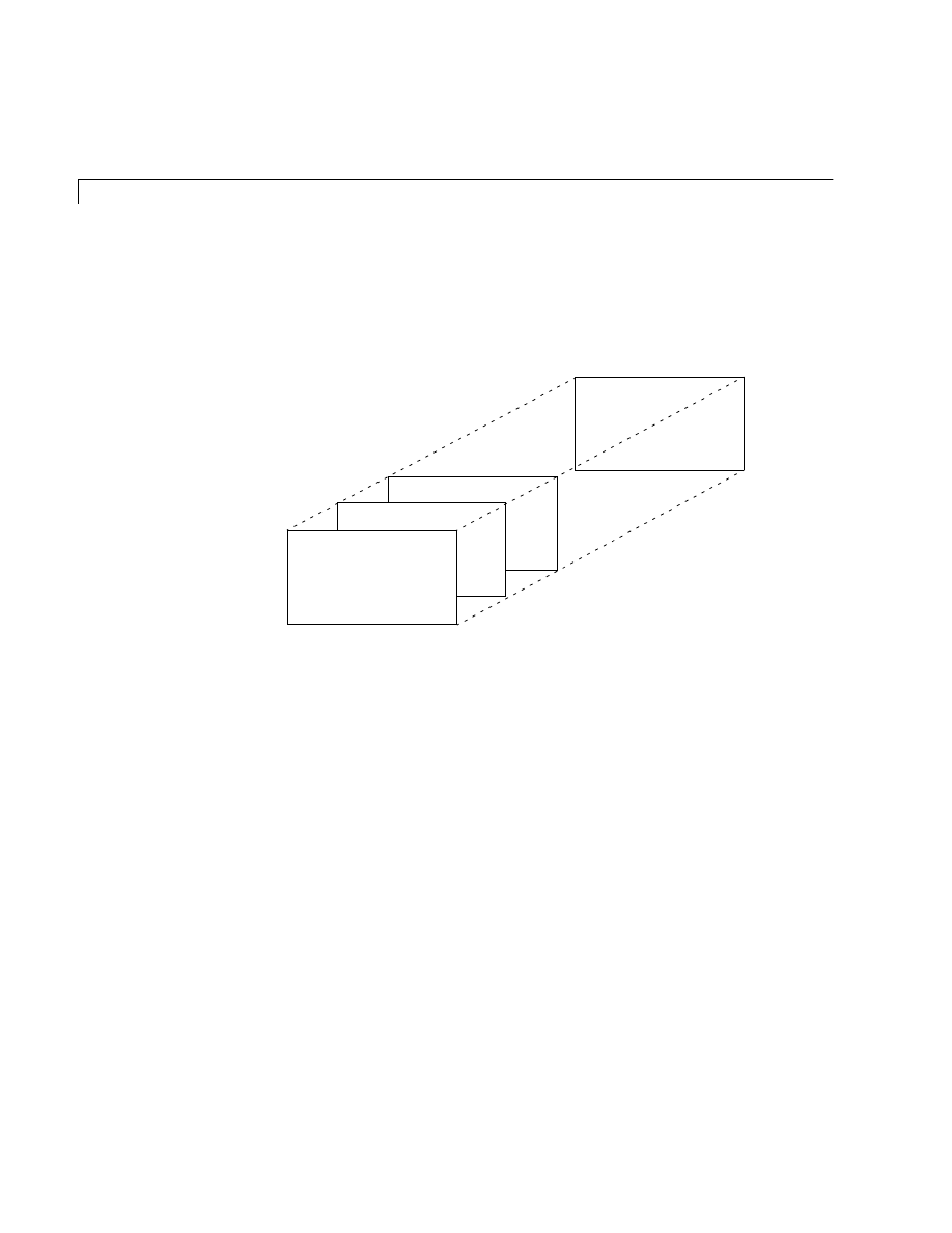
Getting Started
58
stores the sequence of 24 magic squares in a three-dimensional array,
M
. The
size of
M
is
size(M)
ans =
4 4 24
It turns out that the 22nd matrix in the sequence is Dürer’s:
M(:,:,22)
ans =
16 3 2 13
5 10 11 8
9 6 7 12
4 15 14 1
The statement
sum(M,d)
computes sums by varying the
d
th subscript. So
sum(M,1)
is a 1-by-4-by-24 array containing 24 copies of the row vector
34 34 34 34
13 2 3 16
8 11 10 5
12 7 6 9
1 14 15 4
3 13 2 16
10 8 11 5
6 12 7 9
15 1 14 4
16 2 3 13
5 11 10 8
9 7 6 12
4 14 15 1
13 3 2 16
8 10 11 5
12 6 7 9
1 15 14 4
..
.

Other Data Structures
59
and
sum(M,2)
is a 4-by-1-by-24 array containing 24 copies of the column vector
34
34
34
34
Finally,
S = sum(M,3)
adds the 24 matrices in the sequence. The result has size 4-by-4-by-1, so it looks
like a 4-by-4 array,
S =
204 204 204 204
204 204 204 204
204 204 204 204
204 204 204 204
Cell Arrays
Cell arrays in MATLAB are multidimensional arrays whose elements are
copies of other arrays. A cell array of empty matrices can be created with the
cell
function. But, more often, cell arrays are created by enclosing a
miscellaneous collection of things in curly braces,
{}
. The curly braces are also
used with subscripts to access the contents of various cells. For example
C = {A sum(A) prod(prod(A))}
produces a 1-by-3 cell array. The three cells contain the magic square, the row
vector of column sums, and the product of all its elements. When
C
is displayed,
you see
C =
[4x4 double] [1x4 double] [20922789888000]
This is because the first two cells are too large to print in this limited space, but
the third cell contains only a single number, 16!, so there is room to print it.

Getting Started
60
Here are two important points to remember. First, to retrieve the contents of
one of the cells, use subscripts in curly braces. For example,
C{1}
retrieves the
magic square and
C{3}
is 16!. Second, cell arrays contain copies of other arrays,
not pointers to those arrays. If you subsequently change
A
, nothing happens to
C
.
Three-dimensional arrays can be used to store a sequence of matrices of the
same size. Cell arrays can be used to store a sequences of matrices of different
sizes. For example,
M = cells(8,1);
for n = 1:8
M{n} = magic(n);
end
M
produces a sequence of magic squares of different order,
M =
[ 1]
[ 2x2 double]
[ 3x3 double]
[ 4x4 double]
[ 5x5 double]
[ 6x6 double]
[ 7x7 double]
[ 8x8 double]
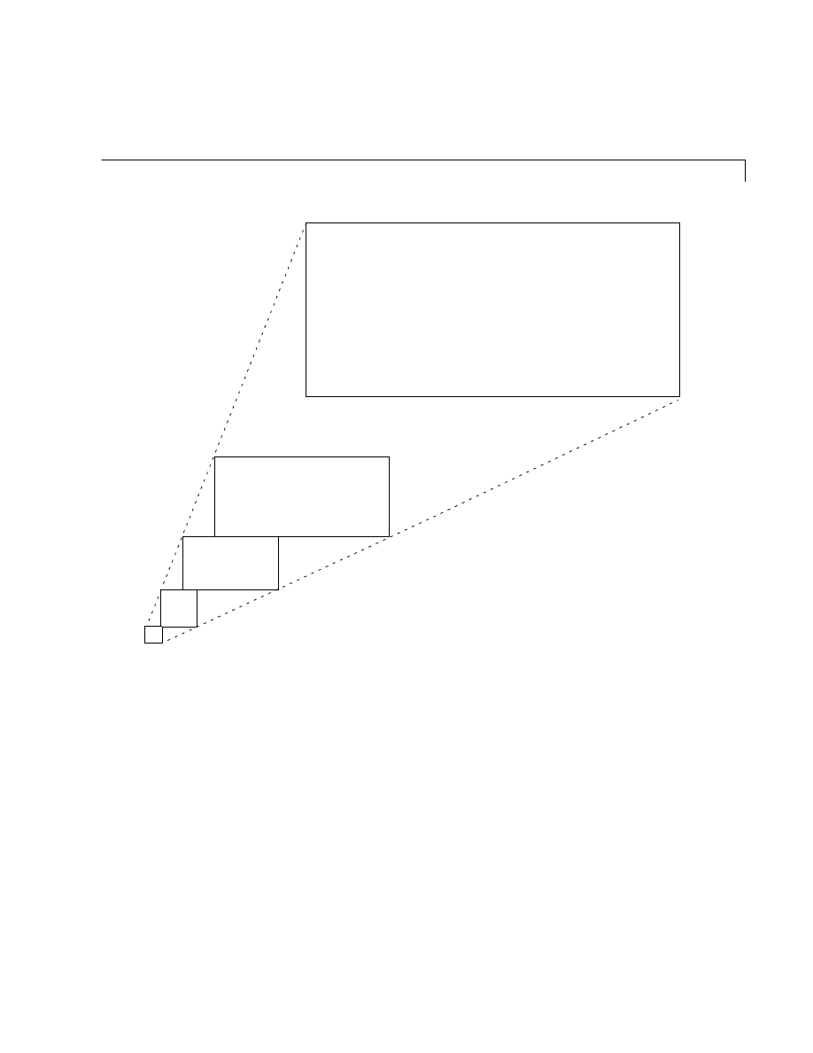
Other Data Structures
61
You can retrieve our old friend with
M{4}
Characters and Text
Enter text into MATLAB using single quotes. For example,
s = 'Hello'
The result is not the same kind of numeric matrix or array we have been
dealing with up to now. It is a 1-by-5 character array.
16 2 3 13
5 11 10 8
9 7 6 12
4 14 15 1
...
64
2
3
61
60
6
7
57
9
55
54
12
13
51
50
16
17
47
46
20
21
43
42
24
40
26
27
37
36
30
31
33
32
34
35
29
28
38
39
25
41
23
22
44
45
19
18
48
49
15
14
52
53
11
10
56
8
58
59
5
4
62
63
1
1 3
4 2
8 1 6
3 5 7
4 9 2
1

Getting Started
62
Internally, the characters are stored as numbers, but not in floating-point
format. The statement
a = double(s)
converts the character array to a numeric matrix containing floating-point
representations of the ASCII codes for each character. The result is
a =
72 101 108 108 111
The statement
s = char(a)
reverses the conversion.
Converting numbers to characters makes it possible to investigate the various
fonts available on your computer. The printable characters in the basic ASCII
character set are represented by the integers
32:127
. (The integers less than
32 represent nonprintable control characters.) These integers are arranged in
an appropriate 6-by-16 array with
F = reshape(32:127,16,6)';
The printable characters in the extended ASCII character set are represented
by
F+128
. When these integers are interpreted as characters, the result
depends on the font currently being used. Type the statements
char(F)
char(F+128)
and then vary the font being used for the MATLAB command window. On a PC,
select Preferences under the File menu. Be sure to try the Symbol and

Other Data Structures
63
Wingdings
fonts, if you have them on your computer. Here is one example of
the kind of output you might obtain.
!"#$%&'()*+,-./
0123456789:;<=>?
@ABCDEFGHIJKLMNO
PQRSTUVWXYZ[\]^_
`abcdefghijklmno
pqrstuvwxyz{|}~-
†°¢£§•¶ß®©™´¨¦ÆØ
×±ðŠ¥µ¹²³¼½ªº¾æø
¿¡¬ÐƒÝý«»…þÀÃÕŒœ
–—“”‘’÷ÞÿŸ
⁄
¤‹›__
‡·‚„‰ÂÊÁËÈÍÎÏÌÓÔ
šÒÚÛÙiˆ˜¯``°¸
″
`ÿ
Concatenation with square brackets joins text variables together into larger
strings. The statement
h = [s, ' world']
joins the strings horizontally and produces
h =
Hello world
The statement
v = [s; 'world']
joins the strings vertically and produces
v =
Hello
world
Note that a blank has to be inserted before the
'w'
in
h
and that both words in
v
have to have the same length. The resulting arrays are both character arrays;
h
is 1-by-11 and
v
is 2-by-5.
To manipulate a body of text containing lines of different lengths, you have two
choices – a padded character array or a cell array of strings. The
char
function
accepts any number of lines, adds blanks to each line to make them all the

Getting Started
64
same length, and forms a character array with each line in a separate row. For
example
S = char('A','rolling','stone','gathers','momentum.')
produces a 5-by-9 character array
S =
A
rolling
stone
gathers
momentum.
There are enough blanks in each of the first four rows of
S
to make all the rows
the same length. Alternatively, you can store the text in a cell array. For
example
C = {'A';'rolling';'stone';'gathers';'momentum.'}
is a 5-by-1 cell array
C =
'A'
'rolling'
'stone'
'gathers'
'momentum.'
You can convert a padded character array to a cell array of strings with
C = cellstr(S)
and reverse the process with
S = char(C)
Structures
Structures are multidimensional MATLAB arrays with elements accessed by
textual field designators. For example,
S.name = 'Ed Plum';
S.score = 83;
S.grade = 'B+'

Other Data Structures
65
creates a scalar structure with three fields.
S =
name: 'Ed Plum'
score: 83
grade: 'B+'
Like everything else in MATLAB, structures are arrays, so you can insert
additional elements. In this case, each element of the array is a structure with
several fields. The fields can be added one at a time,
S(2).name = 'Toni Miller';
S(2).score = 91;
S(2).grade = 'A–';
Or, an entire element can be added with a single statement.
S(3) = struct('name','Jerry Garcia',...
'score',70,'grade','C')
Now the structure is large enough that only a summary is printed.
S =
1x3 struct array with fields:
name
score
grade
There are several ways to reassemble the various fields into other MATLAB
arrays. They are all based on the notation of a comma separated list. If you type
S.score
it is the same as typing
S(1).score, S(2).score, S(3).score
This is a comma separated list. Without any other punctuation, it is not very
useful. It assigns the three scores, one at a time, to the default variable
ans
and
dutifully prints out the result of each assignment. But when you enclose the
expression in square brackets,
[S.score]

Getting Started
66
it is the same as
[S(1).score, S(2).score, S(3).score]
which produces a numeric row vector containing all of the scores.
ans =
83 91 70
Similarly, typing
S.name
just assigns the names, one at time, to
ans
. But enclosing the expression in
curly braces,
{S.name}
creates a 1-by-3 cell array containing the three names.
ans =
'Ed Plum' 'Toni Miller' 'Jerry Garcia'
And
char(S.name)
calls the
char
function with three arguments to create a character array from
the
name
fields,
ans =
Ed Plum
Toni Miller
Jerry Garcia

Scripts and Functions
67
Scripts and Functions
MATLAB is a powerful programming language as well as an interactive
computational environment. Files that contain code in the MATLAB language
are called M-files. You create M-files using a text editor, then use them as you
would any other MATLAB function or command.
There are two kinds of M-files:
• Scripts, which do not accept input arguments or return output arguments.
They operate on data in the workspace.
• Functions, which can accept input arguments and return output arguments.
Internal variables are local to the function.
If you’re a new MATLAB programmer, just create the M-files that you want to
try out in the current directory. As you develop more of your own M-files, you
will want to organize them into other directories and personal toolboxes that
you can add to MATLAB’s search path.
If you duplicate function names, MATLAB executes the one that occurs first in
the search path.
To view the contents of an M-file, for example,
myfunction.m
, use
type myfunction
Scripts
When you invoke a script, MATLAB simply executes the commands found in
the file. Scripts can operate on existing data in the workspace, or they can
create new data on which to operate. Although scripts do not return output
arguments, any variables that they create remain in the workspace, to be used
in subsequent computations. In addition, scripts can produce graphical output
using functions like
plot
.
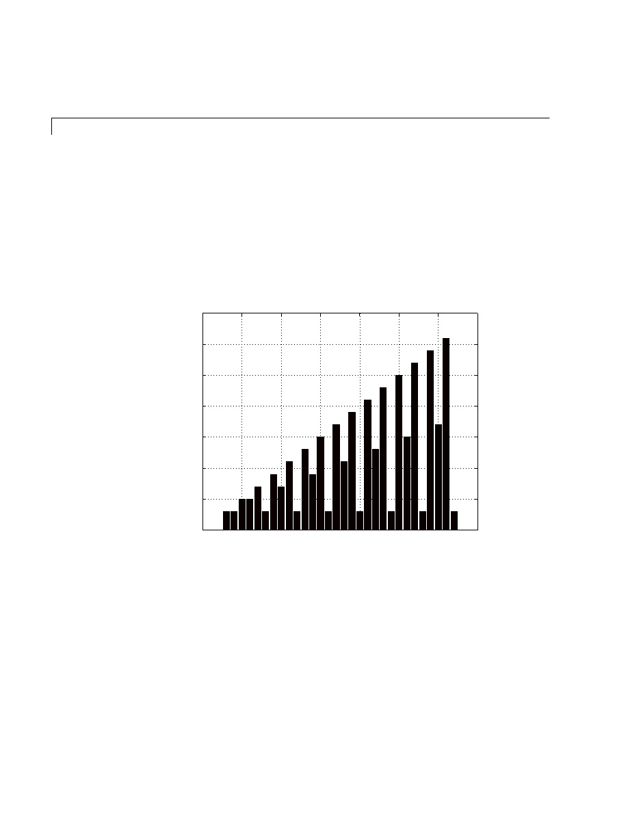
Getting Started
68
For example, create a file called
magicrank.m
that contains these MATLAB
commands:
% Investigate the rank of magic squares
r = zeros(1,32);
for n = 3:32
r(n) = rank(magic(n));
end
r
bar(r)
Typing the statement
magicrank
causes MATLAB to execute the commands, compute the rank of the first 30
magic squares, and plot a bar graph of the result. After execution of the file is
complete, the variables
n
and
r
remain in the workspace.
0
5
10
15
20
25
30
35
0
5
10
15
20
25
30
35

Scripts and Functions
69
Functions
Functions are M-files that can accept input arguments and return output
arguments. The name of the M-file and of the function should be the same.
Functions operate on variables within their own workspace, separate from the
workspace you access at the MATLAB command prompt.
A good example is provided by
rank
. The M-file
rank.m
is available in the
directory
toolbox/matlab/matfun
You can see the file with
type rank
Here is the file.
function r = rank(A,tol)
% RANK Matrix rank.
% RANK(A) provides an estimate of the number of linearly
% independent rows or columns of a matrix A.
% RANK(A,tol) is the number of singular values of A
% that are larger than tol.
% RANK(A) uses the default tol = max(size(A)) * norm(A) * eps.
s = svd(A);
if nargin==1
tol = max(size(A)) * max(s) * eps;
end
r = sum(s > tol);
The first line of a function M-file starts with the keyword
function
. It gives the
function name and order of arguments. In this case, there are up to two input
arguments and one output argument.
The next several lines, up to the first blank or executable line, are comment
lines that provide the help text. These lines are printed when you type
help rank
The first line of the help text is the H1 line, which MATLAB displays when you
use the
lookfor
command or request
help
on a directory.

Getting Started
70
The rest of the file is the executable MATLAB code defining the function. The
variable
s
introduced in the body of the function, as well as the variables on the
first line,
r
,
A
and
tol
, are all local to the function; they are separate from any
variables in the MATLAB workspace.
This example illustrates one aspect of MATLAB functions that is not ordinarily
found in other programming languages – a variable number of arguments. The
rank
function can be used in several different ways:
rank(A)
r = rank(A)
r = rank(A,1.e–6)
Many M-files work this way. If no output argument is supplied, the result is
stored in
ans
. If the second input argument is not supplied, the function
computes a default value. Within the body of the function, two quantities
named
nargin
and
nargout
are available which tell you the number of input
and output arguments involved in each particular use of the function. The
rank
function uses
nargin
, but does not need to use
nargout
.
Global Variables
If you want more than one function to share a single copy of a variable, simply
declare the variable as
global
in all the functions. Do the same thing at the
command line if you want the base workspace to access the variable. The global
declaration must occur before the variable is actually used in a function.
Although it is not required, using capital letters for the names of global
variables helps distinguish them from other variables. For example, create an
M-file called
falling.m
:
function h = falling(t)
global GRAVITY
h = 1/2*GRAVITY*t.^2;
Then interactively enter the statements:
global GRAVITY
GRAVITY = 32;
y = falling((0:.1:5)');
The two global statements make the value assigned to
GRAVITY
at the
command prompt available inside the function. You can then modify
GRAVITY
interactively and obtain new solutions without editing any files.

Scripts and Functions
71
Command/Function Duality
MATLAB commands are statements like
load
help
Many commands accept modifiers that specify operands.
load August17.dat
help magic
type rank
An alternate method of supplying the command modifiers makes them string
arguments of functions.
load('August17.dat')
help('magic')
type('rank')
This is MATLAB’s “command/function duality.” Any command of the form
command argument
can also be written in the functional form
command('argument')
The advantage of the functional approach comes when the string argument is
constructed from other pieces. The following example processes multiple data
files,
August1.dat, August2.dat
, and so on. It uses the function
int2str
,
which converts an integer to a character string, to help build the file name.
for d = 1:31
s = ['August' int2str(d) '.dat']
load(s)
% Process the contents of the d-th file
end
The eval Function
The
eval
function works with text variables to implement a powerful text
macro facility. The expression or statement
eval(s)

Getting Started
72
uses the MATLAB interpreter to evaluate the expression or execute the
statement contained in the text string
s
.
The example of the previous section could also be done with the following code,
although this would be somewhat less efficient because it involves the full
interpreter, not just a function call.
for d = 1:31
s = ['load August' int2char(d) '.dat']
eval(s)
% Process the contents of the d–th file
end
Vectorization
To obtain the most speed out of MATLAB, it’s important to vectorize the
algorithms in your M-files. Where other programming languages might use
for
or
DO
loops, MATLAB can use vector or matrix operations. A simple example
involves creating a table of logarithms.
x = 0;
for k = 1:1001
y(k) = log10(x);
x = x + .01;
end
Experienced MATLAB users
like to say “Life is too short
to spend writing for loops.”
A vectorized version of the same code is
x = 0:.01:10;
y = log10(x);
For more complicated code, vectorization options are not always so obvious.
When speed is important, however, you should always look for ways to
vectorize your algorithms.
Preallocation
If you can’t vectorize a piece of code, you can make your
for
loops go faster by
preallocating any vectors or arrays in which output results are stored. For

Scripts and Functions
73
example, this code uses the function
zeros
to preallocate the vector created in
the
for
loop. This makes the
for
loop execute significantly faster.
r = zeros(32,1);
for n = 1:32
r(n) = rank(magic(n));
end
Without the preallocation in the previous example, the MATLAB interpreter
enlarges the
r
vector by one element each time through the loop. Vector
preallocation eliminates this step and results in faster execution.
Function Functions
A class of functions, called “function functions,” works with nonlinear functions
of a scalar variable. That is, one function works on another function. The
function functions include
• Zero finding
• Optimization
• Quadrature
• Ordinary differential equations
MATLAB represents the nonlinear function by a function M-file. For example,
here is a simplified version of the function
humps
from the
matlab/demos
directory:
function y = humps(x)
y = 1./((x–.3).^2 + .01) + 1./((x–.9).^2 + .04) – 6;
Evaluate this function at a set of points in the interval 0 ð
x
ð 1 with
x = 0:.002:1;
y = humps(x);
Then plot the function with
plot(x,y)
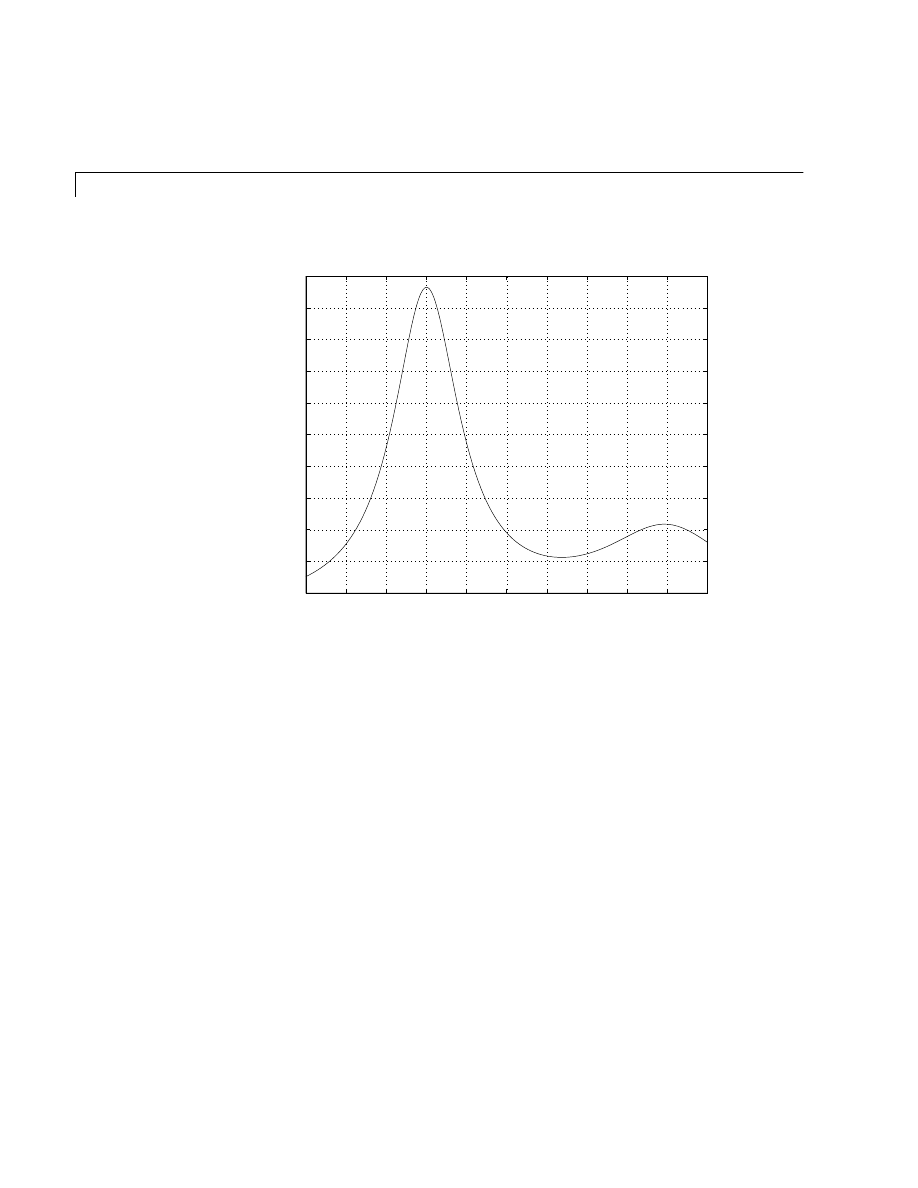
Getting Started
74
The graph shows that the function has a local minimum near x = 0.6. The
function
fmins
finds the minimizer, the value of x where the function takes on
this minimum. The first argument to
fmins
is the name of the function being
minimized and the second argument is a rough guess at the location of the
minimum.
p = fmins('humps',.5)
p =
0.6370
To evaluate the function at the minimizer,
humps(p)
ans =
11.2528
Numerical analysts use the terms quadrature and integration to distinguish
between numerical approximation of definite integrals and numerical
0
0.1
0.2
0.3
0.4
0.5
0.6
0.7
0.8
0.9
1
0
10
20
30
40
50
60
70
80
90
100

Scripts and Functions
75
integration of ordinary differential equations. MATLAB’s quadrature routines
are
quad
and
quad8
. The statement
Q = quad8('humps',0,1)
computes the area under the curve in the graph and produces
Q =
29.8583
Finally, the graph shows that the function is never zero on this interval. So, if
you search for a zero with
z = fzero('humps',.5)
you will find one outside of the interval
z =
–0.1316

Getting Started
76
Handle Graphics
MATLAB provides a set of low-level functions that allows you to create and
manipulate lines, surfaces, and other graphics objects. This system is called
Handle Graphics.
Graphics Objects
Graphics objects are the basic drawing primitives of MATLAB’s Handle
Graphics system. The objects are organized in a tree structured hierarchy. This
reflects the interdependence of the graphics objects. For example, Line objects
require Axes objects as a frame of reference. In turn, Axes objects exist only
within Figure objects.
Graphics Objects
There are eleven kinds of Handle Graphics objects:
• The Root object is the at top of the hierarchy. It corresponds to the computer
screen. MATLAB automatically creates the Root object at the beginning of a
session.
• Figure objects are the windows on the root screen other than the Command
window.
• Uicontrol objects are user interface controls that execute a function when
users activate the object. These include pushbuttons, radio buttons, and
sliders.
• Axes objects define a region in a figure window and orient their children
within this region.
• Uimenu objects are user interface menus that reside at the top of the figure
window.
• Image objects are two-dimensional objects that MATLAB displays using the
elements of a rectangular array as indices into a colormap.
• Line objects are the basic graphics primitive for most two-dimensional plots.
• Patch objects are filled polygons with edges. A single Patch can contain
multiple faces, each colored independently with solid or interpolated colors.
• Surface objects are three-dimensional representations of matrix data created
by plotting the value of the data as heights above the x-y plane.

Handle Graphics
77
• Text objects are character strings.
• Light objects define light sources that affect all objects within the Axes.
Object Handles
Every individual graphics object has a unique identifier, called a handle, that
MATLAB assigns to the object when it is created. Some graphs, such as
multiple line plots, are composed of multiple objects, each of which has its own
handle. Rather than attempting to read handles off the screen and retype
them, you will find that it is always better to store the value in a variable and
pass that variable whenever a handle is required.
The handle of the root object is always zero. The handle of a figure is an integer
that, by default, is displayed in the window title. Other object handles are
floating-point numbers that contain information used by MATLAB. For
example, if
A
is the Dürer magic square, then
h = plot(A)
creates a line plot with four lines, one for each column of
A
. It also returns a
vector of handles such as
h =
9.00024414062500
6.00048828125000
7.00036621093750
8.00036621093750
The actual numerical values are irrelevant and may vary from system to
system. Whatever the numbers are, the important fact is that
h(1)
is the
handle for the first line in the plot,
h(2)
is the handle for the second, and so on.
MATLAB provides several functions to access frequently used object handles:
•
gcf
•
gca
•
gco
You can use these functions as input arguments to other functions that require
figure and axes handles. Obtain the handle of other objects you create at the
time of creation. All MATLAB functions that create objects return the handle
(or a vector of handles) of the object created.

Getting Started
78
Remove an object using the
delete
function, passing the object’s handle as an
argument. For example, delete the current axes (and all of its children) with
the statement:
delete(gca)
Object Creation Functions
Calling the function named after any object creates one of those objects. For
example, the
text
function creates text objects, the
figure
function creates
figure objects, and so on. MATLAB’s high-level graphics functions (like
plot
and
surf
) call the appropriate low-level function to draw their respective
graphics.
Low-level functions simply create one of the eleven graphics objects defined by
MATLAB with the exception of the root object, which only MATLAB can create.
For example:
line([1 3 6], [8 –2 0], 'Color', 'red')
Object Properties
All objects have properties that control how they are displayed. MATLAB
provides two mechanisms for setting the values of properties. Object properties
can be set by the object creation function, or can be changed with the
set
function after the object already exists. For example, these statements create
three objects and override some of their default properties.
days = ['Su';'Mo';'Tu';'We';'Th';'Fr';'Sa']
temp = [21.1 22.2 19.4 23.3 23.9 21.1 20.0];
f = figure
a = axes('YLim',[16 26],'Xtick',1:7,'XTickLabel',days)
h = line(1:7,temp)
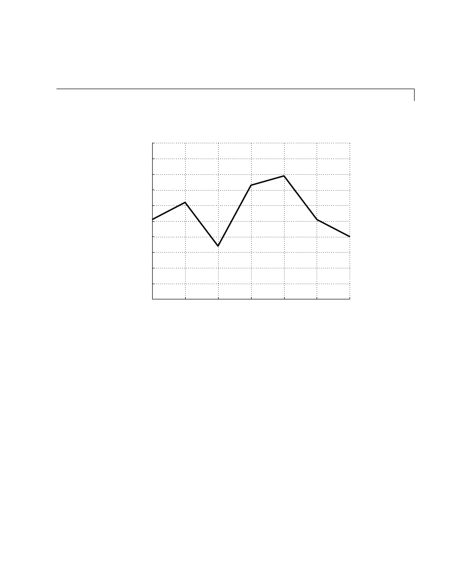
Handle Graphics
79
days
is a character array containing abbreviations for the days of the week and
temp
is a numeric array of typical temperatures. The figure window is created
by calling
figure
with no arguments, so it has the default properties. The axes
exists within the figure and has a specified range for the scaling of the y-axis
and specified labels for the tick marks on the x-axis. The line exists within the
axes and has specified values for the x and y data. The three object handles
f
,
a
, and
h
, are saved for later use.
set and get
Object properties are specified by referencing the object after its creation. To
do this, use the handle returned by the creating function.
The
set
function allows you to set any object’s property by specifying the
object’s handle and any number of property name/property value pairs. For
instance, to change the color and width of the line from the previous example,
set(h,'Color',[0 .8 .8],'LineWidth',3)
Su
Mo
Tu
We
Th
Fr
Sa
16
17
18
19
20
21
22
23
24
25
26
Temperature

Getting Started
80
To see a list of all settable properties for a particular object, call
set
with the
object’s handle:
set(h)
Color
EraseMode: [ {normal} | background | xor | none ]
LineStyle: [ {–} | –– | : | –. | none ]
LineWidth
Marker:
MarkerSize
...
XData
YData
ZData
To see a list of all current settings properties for a particular object, call
get
with the object’s handles:
get(h)
Color = [0 0.8 0.8]
EraseMode = normal
LineStyle =
LineWidth = [3]
Marker = none
MarkerSize = [6]
...
XData = [ (1 by 7) double array]
YData = [ (1 by 7) double array]
ZData = []
To query the value of a property, use
get
with the property name:
get(h,'Color')
ans =
0 0.8000 0.8000

Handle Graphics
81
The axes object carries many of the detailed properties of the overall graphic.
For example, the title is another child of the axes. The statements:
t = get(a,'title');
set(t,'String','Temperature','FontAngle','oblique')
specify a particular title. The
title
function provides another interface to the
same properties.
Graphics User Interfaces
Here is a simple example illustrating how to use Handle Graphics to build user
interfaces. The statement
b = uicontrol('Style','pushbutton', ...
'Units','normalized', ...
'Position',[.5 .5 .2 .1], ...
'String','click here');
creates a pushbutton in the center of a figure window and returns a handle to
the new object. But, so far, clicking on the button does nothing. The statement
s = 'set(b,''Position'',[.8*rand .9*rand .2 .1])';
creates a string containing a command that alters the pushbutton’s position.
Repeated execution of
eval(s)
moves the button to random positions. Finally,
set(b,'Callback',s)
installs
s
as the button’s callback action, so every time you click on the button,
it moves to a new position.
Animations
MATLAB provides several ways of generating moving, animated, graphics.
Using the
EraseMode
property is appropriate for long sequences of simple plots
where the change from frame to frame is minimal. Here is an example showing
simulated Brownian motion. Specify a number of points, like
n = 20

Getting Started
82
and a temperature or velocity, such as
s = .02
The best values for these two parameters depend upon the speed of your
particular computer. Generate
n
random points with (x,y) coordinates between
–
1
/
2
and +
1
/
2
x = rand(n,1)–0.5;
y = rand(n,1)–0.5;
Plot the points in a square with sides at -1 and +1. Save the handle for the
vector of points and set its
EraseMode
to
xor
. This tells the MATLAB graphics
system not to redraw the entire plot when the coordinates of one point are
changed, but to restore the background color in the vicinity of the point using
an “exclusive or” operation.
h = plot(x,y,'.');
axis([–1 1 –1 1])
axis square
grid off
set(h,'EraseMode','xor','MarkerSize',18)
Now begin the animation. Here is an infinite
while
loop, which you will
eventually break out of by typing
<ctrl>–c
. Each time through the loop, add a
small amount of normally distributed random noise to the coordinates of the
points. Then, instead of creating an entirely new plot, simply change the
XData
and
YData
properties of the original plot.
while 1
drawnow
x = x + s*randn(n,1);
y = y + s*randn(n,1);
set(h,'XData',x,'YData',y)
end
How long does it take for one of the points to get outside of the square? How
long before all of the points are outside the square?
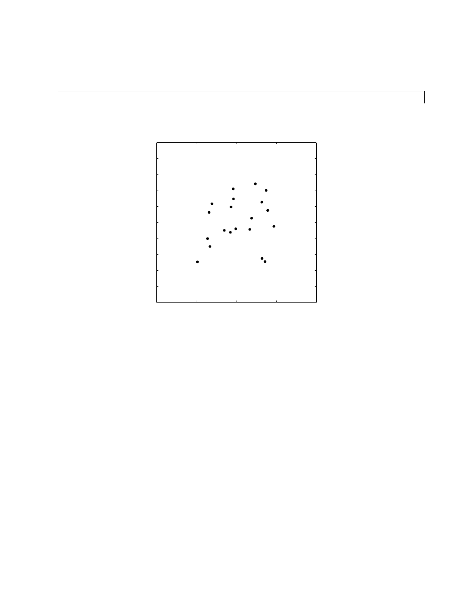
Handle Graphics
83
Movies
If you increase the number of points in the Brownian motion example to
something like
n = 300
and
s = .02
, the motion is no longer very fluid; it takes
too much time to draw each time step. It becomes more effective to save a
predetermined number of frames as bitmaps and to play them back as a movie.
First, decide on the number of frames, say
nframes = 50;
Next, set up the first plot as before, except do not use
EraseMode
.
x = rand(n,1)–0.5;
y = rand(n,1)–0.5;
h = plot(x,y,'.')
set(h,'MarkerSize',18);
axis([–1 1 –1 1])
axis square
grid off
−1
−0.5
0
0.5
1
−1
−0.8
−0.6
−0.4
−0.2
0
0.2
0.4
0.6
0.8
1

Getting Started
84
Now, allocate enough memory to save the complete movie,
M = moviein(nframes);
This sets aside a large matrix with
nframes
columns. Each column is long
enough to save one frame. The total amount of memory required is proportional
to the number of frames, and to the area of the current axes; it is independent
of the complexity of the particular plot. For 50 frames and the default axes,
over 7.5 megabytes of memory is required. This example is using square axes,
which is slightly smaller, so only about 6 megabytes is required.
Generate the movie and use
getframe
to capture each frame.
for k = 1:nframes
x = x + s*randn(n,1);
y = y + s*randn(n,1);
set(h,'XData',x,'YData',y)
M(:,k) = getframe;
end
Finally, play the movie 30 times.
movie(M,30)

Learning More
85
Learning More
To see more MATLAB examples, select Examples and Demos under the menu,
or type
demo
at the MATLAB prompt. From the menu displayed, run the demos that interest
you, and follow the instructions on the screen.
For a more detailed explanation of any of the topics covered in this book, see
• The MATLAB Installation Guide describes how to install MATLAB on your
platform.
• Using MATLAB provides in depth material on the MATLAB language,
working environment, and mathematical topics.
• Using MATLAB Graphics describes how to use MATLAB’s graphics and
visualization tools.
• The MATLAB Application Program Interface Guide explains how to write C
or Fortran programs that interact with MATLAB.
• MATLAB Product Family New Features provides information on what is new
in this release and information that is useful in making the transition from
previous releases of MATLAB to this release.
MATLAB Toolboxes are collections of M-files that extend MATLAB's
capabilities to a number of technical fields. Separate guides are available for
each of the Toolboxes. Some of the topics they cover are
Communications
Control Systems
Financial Computation
Frequency-Domain System Identification
Fuzzy Logic
Higher-Order Spectral Analysis
Image Processing
Linear Matrix Inequalities

Getting Started
86
Model Predictive Control
Mu-Analysis and Synthesis
Numerical Algorithms
Neural Networks
Optimization
Partial Differential Equations
Quantitative Feedback Theory
Robust Control
Signal Processing
Simulation (Simulink)
Splines
Statistics
Symbolic Mathematics
System Identification
Wavelets
For the very latest information about MATLAB and other MathWorks
products, point your Web browser to:
http://www.mathworks.com
and use your Internet News reader to access the newsgroup
comp.soft-sys.matlab
A number of MATLAB-related books available from many different publishers.
A booklet entitled MATLAB-Based Books is available from The MathWorks
and an up-to-date list is available on the Web site.
If you have read this entire book and run all the examples, congratulations, you
are off to a great start with MATLAB. If you have skipped to this last section
or haven’t tried any of the examples, may we suggest you spend a little more
time Getting Started. In either case, welcome to the world of MATLAB!

I-1
Index
A
animation 81
API vii
arrays 42, 45
cell 59
columnwise organization 47
concatenating 17
creating in M-files 16
deleting rows or columns 17
elements 11
generating with functions and operators 15
listing contents 11
loading from external data files 16
multidimensional 57
notation for elements 11
variable names 11
C
cell arrays 59
colon operator 8
command line editing 21
concatenating arrays 17
continuing statements on multiple lines 21
D
doc
E
editing command lines 21
elements of arrays 11
external programs
F
file manipulation 40
flow control 52
for
format
function functions 73
functions 12, 69
G
global variables 70
graphics
2-D 23
handle graphics 76
objects 76
H
Handle Graphics vii, 76
help 34
I
if

Index
I-2
L
library
loading arrays 16
logical vectors 49
lookfor
M
mathematical function library vii
MATLAB
Application Programmer’s Interface vii
Handle Graphics vii
history vi
language vii
mathematical function library vii
overview vi
starting 2
working environment vii
matrix 3
M-file
movies 83
multidimensional arrays 57
multivariate data, organizing 47
N
O
objects, graphics 76
online help
operators 12
output
controlling format 19
suppressing 21
P
plotting
preallocation 72
printing
graphics 33
online reference pages 37
R
Reference Guide 34
running external programs 41
S
save
scripts 67
search path 39
searching online help 36, 37
semicolon to suppress output 21
Simulink vii
starting MATLAB 2
statements

Index
I-3
subplot
subscripting
sum
switch
T
transpose
U
user interfaces
V
vector
W
while
who
working environment
workspace
Document Outline
- Introduction
- Getting Started
- Index
Wyszukiwarka
Podobne podstrony:
(ebook pdf) Matlab Getting started
(ebook pdf) Matlab Getting started
Getting Started
getting started IAOTAGZXANHHC6G Nieznany
Part I Getting Started
1 3 Getting started with Data Studio Lab
Getting Started with PostHASTE
Packt Publishing Getting Started with Backbone Marionette (2014)
Getting Started
ANSYS Getting Started Tutorial Workbench
chinas southwest 3 getting started
1 2 Getting started (2)
Neuro Solutions 5 Getting Started Manual
mr zr getting started
01 GETTING STARTED
Part I Getting Started
więcej podobnych podstron