
NeuroSolutions
Getting Started Manual
Version 5

ii

iii
Table of Contents
CHAPTER 1: WELCOME ..................................................................................................... 1
1.1 W
ELCOME TO
N
EURO
S
OLUTIONS
.................................................................................. 1
1.2 L
EVEL
S
UMMARY
.......................................................................................................... 1
1.3 T
ECHNICAL
S
UPPORT
.................................................................................................... 3
1.4 O
THER
N
EURO
D
IMENSION
P
RODUCTS
.......................................................................... 4
CHAPTER 2: INSTALLATION ............................................................................................ 8
2.1 P
ACKING
L
IST
............................................................................................................... 8
2.2 S
YSTEM
R
EQUIREMENTS
............................................................................................... 8
2.3 I
NSTALLATION
I
NSTRUCTIONS
...................................................................................... 8
2.4 S
UMMARY OF
I
NSTALLED
C
OMPONENTS
....................................................................... 9
2.5 U
NINSTALLING
N
EURO
S
OLUTIONS
............................................................................. 10
CHAPTER 3: LEARNING ABOUT NEUROSOLUTIONS .............................................. 11
3.1 S
TARTING
N
EURO
S
OLUTIONS
..................................................................................... 11
3.2 R
UNNING THE
D
EMOS
................................................................................................. 11
3.3 U
SING THE
O
NLINE
H
ELP
............................................................................................ 13
CHAPTER 4: BUILDING A NEURAL NETWORK ......................................................... 15
4.1 F
OUR
W
AYS TO
C
ONSTRUCT A
N
EURAL
N
ETWORK
.................................................... 15
4.2 T
HE
N
EURAL
E
XPERT
.................................................................................................. 16
4.2.1 Starting
the
NeuralExpert .................................................................................... 16
4.2.2 Getting
Help
in
the NeuralExpert ........................................................................ 17
4.2.3 NeuralExpert
Problem
Type Selection Panel....................................................... 17
4.2.4 NeuralExpert
Input
File Selection Panel ............................................................. 18
4.2.5 NeuralExpert
Tag
Input Columns Panel .............................................................. 19
4.2.6 NeuralExpert
Desired
File Selection Panel ......................................................... 20
4.2.7
NeuralExpert Tag Desired Columns Panel.......................................................... 21
4.2.8
NeuralExpert Tag Symbolic Desired Panel ......................................................... 22
4.2.9 NeuralExpert
Generalization Protection Panel ................................................... 23
4.2.10
NeuralExpert Out Of Sample Testing Panel ........................................................ 24
4.2.11 NeuralExpert
Network Complexity Panel ............................................................ 25
CHAPTER 5: UNDERSTANDING THE BREADBOARD ............................................... 27
5.1 B
READBOARD
I
CONS
................................................................................................... 27
5.2 T
HE
I
NSPECTOR
........................................................................................................... 29

iv
CHAPTER 6: TRAINING A NETWORK........................................................................... 32
6.1 R
UNNING A
S
IMULATION
............................................................................................. 32
6.2 R
ECOVERING FROM AN
U
NSUCCESSFUL
T
RAINING
..................................................... 34
6.3 V
ERIFYING THE
T
RAINING
........................................................................................... 36
6.4 D
ENORMALIZING THE
P
ROBES
.................................................................................... 36
6.5 M
ANUALLY
O
PTIMIZING THE
N
ETWORK
..................................................................... 37
CHAPTER 7: TESTING A NETWORK ............................................................................. 39
7.1 S
TARTING THE
T
ESTING
W
IZARD
................................................................................. 39
7.2 G
ETTING
H
ELP IN THE
T
ESTING
W
IZARD
..................................................................... 39
7.3 T
ESTING
W
IZARD
D
ATA
S
ET
S
ELECTION
P
ANEL
.......................................................... 40
7.4 T
ESTING
W
IZARD
O
UTPUT
P
RODUCTION
P
ANEL
.......................................................... 41
CHAPTER 8: THE NEURALBUILDER............................................................................. 42
8.1 S
TARTING THE
N
EURAL
B
UILDER
................................................................................ 42
8.2 G
ETTING
H
ELP IN THE
N
EURAL
B
UILDER
..................................................................... 43
8.3 N
EURAL
B
UILDER
S
UPPORTED
M
ODELS
...................................................................... 43
8.4 N
EURAL
B
UILDER
T
RAINING
D
ATA
P
ANEL
.................................................................. 44
8.5 C
ROSS
V
ALIDATION AND
T
EST
D
ATA
P
ANEL
.............................................................. 46
8.6 N
EURAL
B
UILDER
T
OPOLOGY
P
ANEL
.......................................................................... 47
8.7 N
EURAL
B
UILDER
H
IDDEN
L
AYER
P
ANEL
................................................................... 48
8.8 N
EURAL
B
UILDER
O
UTPUT
L
AYER
P
ANEL
................................................................... 50
8.9 N
EURAL
B
UILDER
S
UPERVISED
L
EARNING
P
ANEL
....................................................... 52
8.10 N
EURAL
B
UILDER
P
ROBE
C
ONFIGURATION
P
ANEL
...................................................... 53
8.11 B
UILDING THE
N
ETWORK WITH THE
N
EURAL
B
UILDER
............................................... 55
CHAPTER 9: NEURAL NETWORK THEORY................................................................ 56
9.1 S
UMMARY OF
N
EURAL
N
ETWORK
T
HEORY
................................................................ 56
9.2 T
HE
N
EURAL
N
ETWORK
D
ESIGN AND
U
SE
L
IFE
C
YCLE
.............................................. 57
9.3 C
HOOSING A
N
EURAL
A
RCHITECTURE
........................................................................ 58
9.4 N
EURAL
N
ETWORK
T
RAINING
H
INTS
.......................................................................... 60
CHAPTER 10: APPENDIX .................................................................................................... 62
10.1 F
ILE
F
ORMAT
R
EQUIREMENTS
.................................................................................... 62

v
NeuroDimension, Inc.
3701 NW 40th Terrace, Suite 1
Gainesville, FL 32606
Phone: 800-ND-IDEAS
Outside U.S.: 352-377-5144
Fax: 352-377-9009
info@nd.com
www.nd.com

vi

1
Chapter 1: W
ELCOME
1.1 W
ELCOME TO
N
EURO
S
OLUTIONS
Welcome to NeuroSolutions, the premier neural network simulation environment.
This manual is designed to get you up and running in the least amount of time possible. It
is a concise summary of the most important topics covered in the extensive online help.
We anticipate you will be able to cover all material in this manual, including examples, in
less than six hours total time.
By the time you finish this manual, you will have developed a basic familiarity with the
NeuroSolutions environment. To learn more about NeuroSolutions' extensive features, as
well as additional tutorials, examples and an introduction to neural computing, please turn
to the online help.
1.2 L
EVEL
S
UMMARY
Features common to all levels:
Icon-based construction of neural networks
Component-level editing of parameters
Macro recording and playback
OLE-compatible server
Online, context-sensitive help
NeuralBuilder and NeuralExpert neural network construction utilities
2
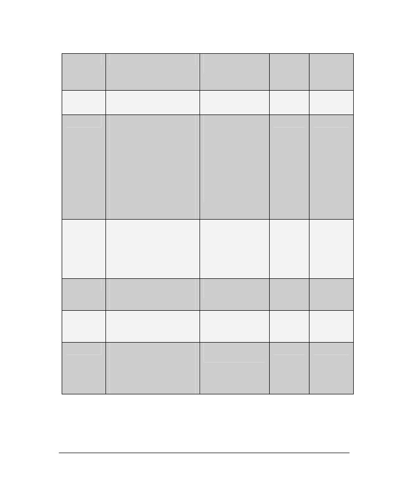
Level-specific features:
Level
Topologies
Learning
Paradigms
Hidden
Layers
Neurons
per
Hidden
Layer
Educator
Multilayer Perceptron (MLP)
Generalized feedforward
Backpropagation
2
50
Users
Educator +
Modular networks
Hebbian
Principal component analysis
(PCA)
Competitive
Kohonen feature maps
Neuro-Fuzzy
Support Vector Machines
Educator +
Unsupervised
Genetic
Adatron (SVM)
Congugate
Gradient
Levenberg-
Marquardt
6
500
Consultants
Users +
Hopfield, time delay
(TDNN)
Time lagged recurrent
(TLRN)
Users +
Backpropagation
through time
(BPTT)
Fixed point
recurrent learning
Unlimited
unlimited
Professional
Consultants +
ANSI C++ Source Code
Generation
Same as
Consultants
Unlimited
unlimited
Developers
Lite
Consultants +
User-defined dynamic link
libraries (DLL’s)
Same as
Consultants
Unlimited
unlimited
Developers
Consultants +
ANSI C++ source code
generation
User-defined dynamic link
libraries (DLL’s)
Same as
Consultants
Unlimited
unlimited
3
1.3 T
ECHNICAL
S
UPPORT
Included with Evaluation/Demo Software
Toll-free line for bug reports and installation problems
Included with Purchased Software
Toll-free line for bug reports and installation problems
90 days of unlimited email, fax and phone support (additional support plans available for purchase)
Contact Information
Bug Reports and Installation Problems:
1-800-634-3327 (option 4)
All other Technical Support:
(352) 377-1542
Fax:
(352) 377-9009
Email:
support@neurosolutions.com
Please have your invoice number ready when calling and include your invoice number in
all fax, email, or written correspondence.
Note that the technical support described above is for questions regarding the software
package. Neural network experts are on staff and available for consulting on an hourly
basis. Consulting rates are dependent on the specifics of the problem.
Help Resources
Before contacting technical support, please attempt to answer any questions by first
consulting the following resources:
This manual
NeuroSolutions Frequently Asked Questions (FAQ)
The online help
The latest versions of the online help and FAQ can always be found at the
NeuroDimension web site: www.nd.com
While we want to encourage you to use the extensive help facilities to answer your
questions, we do not want to discourage you from giving us your feedback on how we can
improve the package and how we can better support you, the customer.

4
1.4 O
THER
N
EURO
D
IMENSION
P
RODUCTS
NeuroSolutions for Excel
NeuroSolutions for Excel is a revolutionary product that allows you access to all the
powerful features of NeuroSolutions, but with the convenience and ease of use of a
spreadsheet program. This Microsoft Excel add-in gives you the ability to visually tag
your data as Training, Cross Validation, Testing, or Production, train a neural network,
and test the neural network's performance directly from within a Microsoft Excel
worksheet. Reports are automatically generated showing the results. Working with neural
networks could not be any easier.
NeuroSolutions for Excel is not just for the novice, however. There are also powerful
built-in features that help you to find the optimum neural network for your problem.
These include the ability to train a neural network multiple times, vary any neural network
parameters across multiple runs, genetically optimize network parameters, and create your
own custom batches.
Custom Solution Wizard
The Custom Solution Wizard is a tool that will take an existing neural network created
with NeuroSolutions and automatically generate and compile a Dynamic Link Library
(DLL). This allows you to easily incorporate neural network models into your own
applications and into other NeuroDimension products, such as TradingSolutions
(Developers level only).
While using the wizard to create the DLL, you are also given the option of creating a shell
for any of the following development environments
1
:
Visual Basic ®
Visual C++ ®
Microsoft Excel ®
Microsoft Access ®
Active Server Pages (Developers level only)
TradingSolutions
Each shell provides a sample application along with source code to give you a starting
point for integrating the generated DLL into your application.
1
® Visual Basic, Visual C++, Microsoft Excel, and Microsoft Access are registered trademarks of Microsoft
Corporation

5
The generated neural network DLL provides a simple protocol for assigning the network
input and producing the corresponding network output. Furthermore, the Developers
level of the Custom Solution Wizard supports learning. This allows you to train the
generated neural network and/or retune the network after gathering new data.
Embedding a custom neural network into your application could not be any easier!
Neural and Adaptive Systems: Fundamentals Through Simulations
This interactive electronic book published by John Wiley and Sons combines the
hypertext and searching capabilities of the Windows help system with the highly graphical
simulation environment of NeuroSolutions to produce a revolutionary learning tool. The
book contains over 200 interactive experiments in NeuroSolutions to elucidate the
fundamentals of neural networks and adaptive systems.
TradingSolutions
TradingSolutions is a comprehensive financial analysis software package that helps you
make better trading decisions. It combines traditional technical analysis with state-of-the-
art artificial intelligence technologies. Now you can use any combination of financial
indicators in conjunction with advanced neural networks and genetic algorithms to create
models that are remarkably effective, especially in today's volatile markets.
TradingSolutions' user-friendly interface allows you to perform complex financial
forecasting without leaving you lost in the technology. Simple wizards guide you step-by-
step through each task, while optional advanced panels give you the flexibility to adjust
parameters behind the scenes.
Genetic Server
Genetic Server is a general-purpose genetic algorithm ActiveX component that can be
used to easily build custom genetic applications in Visual Basic (or any other environment
that supports Active-X components). This software provides two core genetic algorithms:
Generational and Steady State. Furthermore, the user can select between several types of
selection, crossover, and mutation. Floating point and integer data types are supported in
addition to the traditional binary data type. Genetic Server also provides several methods
for terminating the genetic search.
Genetic Library
Genetic Library is a general-purpose genetic algorithm library written in ANSI C++. The
library provides two core genetic algorithms: Generational and Steady State.
Furthermore, the user can select between several types of selection, crossover, and
mutation, or even write their own. Floating point and integer data types are supported in
addition to the traditional binary data type. The library also provides several methods for
terminating the genetic search.

6
Consulting
Neural network and genetic algorithm experts are on staff and available for consulting on
an hourly basis. Consulting rates are dependent upon the specifics of the problem. To
obtain an estimate for consulting, please email your problem specifics to info@nd.com.
Support and Maintenance Packages
2
Gold Support Plan
NeuroDimension offers an extended support plan, called the Gold Support Plan:
•
1-Year of additional email support (1-Year begins after initial 90-Day period)
•
Available anytime
•
Annual subscription price: $195
The annual subscription price for the Gold Support Plan is $135 while in-service.
Platinum Support Plan
NeuroDimension offers an extended support plan, called the Platinum Support Plan:
•
1-Year of additional email and phone support (1-Year begins after initial 90-Day
period)
•
Priority treatment for all support issues
•
Guaranteed bug fixes (or work around) within 5 business days
•
2 sessions (max time: 30-minutes each) of web conference for technical support
related issues
•
$200 coupon towards neural network training course (only valid during duration
of support)
•
Available anytime
•
Annual subscription price: $495
The annual subscription price for the Platinum Support Plan is $345 while in-service.
2
The technical support described above is for questions regarding the software package.
Neural network experts are on staff and available for consulting on an hourly basis.
Consulting rates are dependent on the specifics of the problem.

7
NeuroSolutions Maintenance Plan
NeuroDimension offers an maintenance/upgrade plan, called the NeuroSolutions
Maintenance Plan:
•
1-Year of Free Minor Upgrades and (1) Major Upgrade (1-Year begins after initial
90-Day period)
•
Access to Beta Products
•
Available only within 30 days of product purchase
•
Annual subscription cost: 30% of list price
The annual subscription price for the NeuroSolutions Maintenance Plan is 30% of the
list price of the software. This product is only available within 30 days of the software
purchase.

8
Chapter 2: I
NSTALLATION
2.1 P
ACKING
L
IST
Before installing, verify that you received the following materials:
Compact disk (CD)
Installation instructions page
Technical support page
NeuroSolutions Getting Started Manual
If any components are missing, please contact NeuroDimension immediately.
To ensure that you are kept informed of the latest product updates and releases, please
complete and mail the registration card.
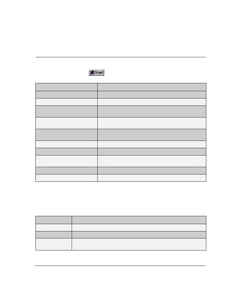
2.2 S
YSTEM
R
EQUIREMENTS
Before installing NeuroSolutions, you should verify that your system configuration meets
the following minimum specifications:
Operating System
Windows 98 or Higher
Mac OS 9/ OS X with Connectix Virtual PC for Mac
Memory
32MB RAM (64MB recommended)
Hard Drive
80MB free disk space
Video
640x480 with 256 colors (800x600 with 16M colors recommended)
2.3 I
NSTALLATION
I
NSTRUCTIONS
1) Install the Software
Insert the CD-ROM into the drive. The installation program should start automatically. If
this does not happen, run the program "autorun.exe" from the root CD directory.
The installation program is highly automated and easy to use. Follow the on-screen
instructions. It is recommended that first-time users perform the typical installation.
2) Activate the Software
9
NeuroSolutions is initially in evaluation mode and must be activated in order to remove
the evaluation restrictions. Once you purchase a license for NeuroSolutions you will
receive an email with instructions for obtaining an activation code that you will use to
activate the software. If you purchased and did not receive this email or have misplaced it,
please contact NeuroDimension to have another copy sent to you.
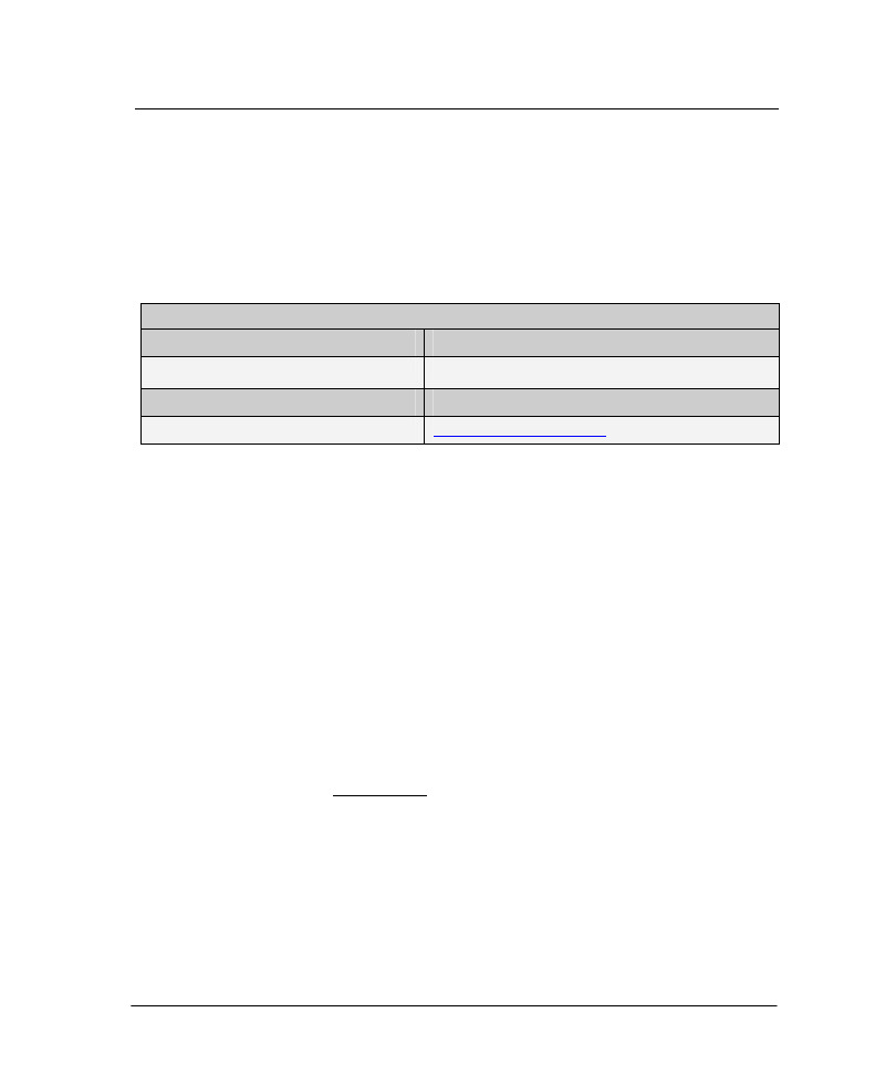
2.4 S
UMMARY OF
I
NSTALLED
C
OMPONENTS
If you have chosen the default installation, NeuroSolutions will install the following items
in the Windows Start Menu
, Start
⇒
Programs
⇒
NeuroSolutions 5:
Item
Description
Data Manager
A utility for importing, analyzing and preprocessing data files
Getting Started Manual
This manual in online form
Interactive Book Preface and TOC
Preface and Table of Contents on an interactive book on neural
networks (Chapter 1 is included)
NeuralBuilder
A utility for constructing neural networks based on the neural
model desired
NeuralExpert
A utility for constructing neural networks based on the application
type
NeuroSolutions for Excel Demos
A demo of an Excel add-in product for NeuroSolutions
NeuroSolutions for Excel Help
Online documentation for NeuroSolutions for Excel
NeuroSolutions for Excel
Launches Microsoft Excel and loads the NeuroSolutions for Excel
add-in
NeuroSolutions
The main NeuroSolutions program
NeuroSolutions Help
Online documentation for NeuroSolutions
If you performed the default installation, the installation program created the directory
"C:\Program Files\NeuroSolutions 5". Within this directory tree are the sub-directories
and files of the NeuroSolutions package. You will not typically need to directly access
most of the sub-directories; however, three are of interest to beginning users:
Sub-Directory
Description
DLLCust
Contains some ready-to-use Dynamic Link Libraries (DLL’s)
Macros
Contains common macros
Tutorials
A set of saved breadboards and related data that correspond to examples in the
online help

10
2.5 U
NINSTALLING
N
EURO
S
OLUTIONS
From the Windows Start Menu
:
Go to Start
⇒
Settings
⇒
Control Panel.
Double-click "Add/Remove Programs".
Select "NeuroSolutions 5" in the list and click the "Add/Remove" button.
Sometimes the uninstall program may leave behind a few files. You may delete these
manually.
11
Chapter 3: L
EARNING
A
BOUT
N
EURO
S
OLUTIONS
3.1 S
TARTING
N
EURO
S
OLUTIONS
The easiest way to start NeuroSolutions is from the Windows Start button
:
Go to Start⇒Programs⇒NeuroSolutions 5⇒NeuroSolutions.
From the Welcome menu that appears, choose
NeuroSolutions under the Demos section.
Demo selection panel
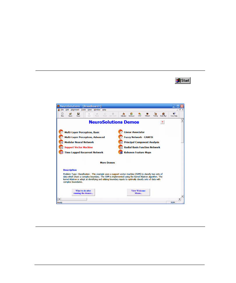
3.2 R
UNNING THE
D
EMOS
The best way to get an overview of the features provided by NeuroSolutions is to run the
demos. These demos present a series of examples in neural computing, which illustrate
the broad range of capabilities NeuroSolutions has to offer.
12
If you have not already launched the
NeuroSolutions Demo panel:
Go to the Help menu and select "Demos," or type "Ctrl+D."
To run a demo,
Make a selection by holding the mouse over the demo title. The selected button's text will turn red,
and the selected demo will be described.
Click the mouse button to run the demo. The demos present a series of panels, each one introducing a
particular feature of NeuroSolutions.
To advance to the next panel, click the Forward button .
To quit the present demo and return to the main demo menu, click the Cancel button .
All demos are live! Each one starts with random initial conditions and learns online. These
demos are also designed to be interactive. Many of the panels have edit cells that allow
you to modify the network parameters and buttons to run the simulation or single-step
through an epoch.
These demos are not restrictive. At any time during the presentation, you are able to
manipulate the breadboard by adding a component, removing a component, or changing a
component’s parameters with the Inspector. This can be advantageous in that you can
learn a lot about the software by experimenting with the components. However, changing
the state of the breadboard may result in an error message later in the demo. If the demo
does fail, click the Cancel button to get you back to main demo menu. Or, simply
restart the demo.
A running demo
13
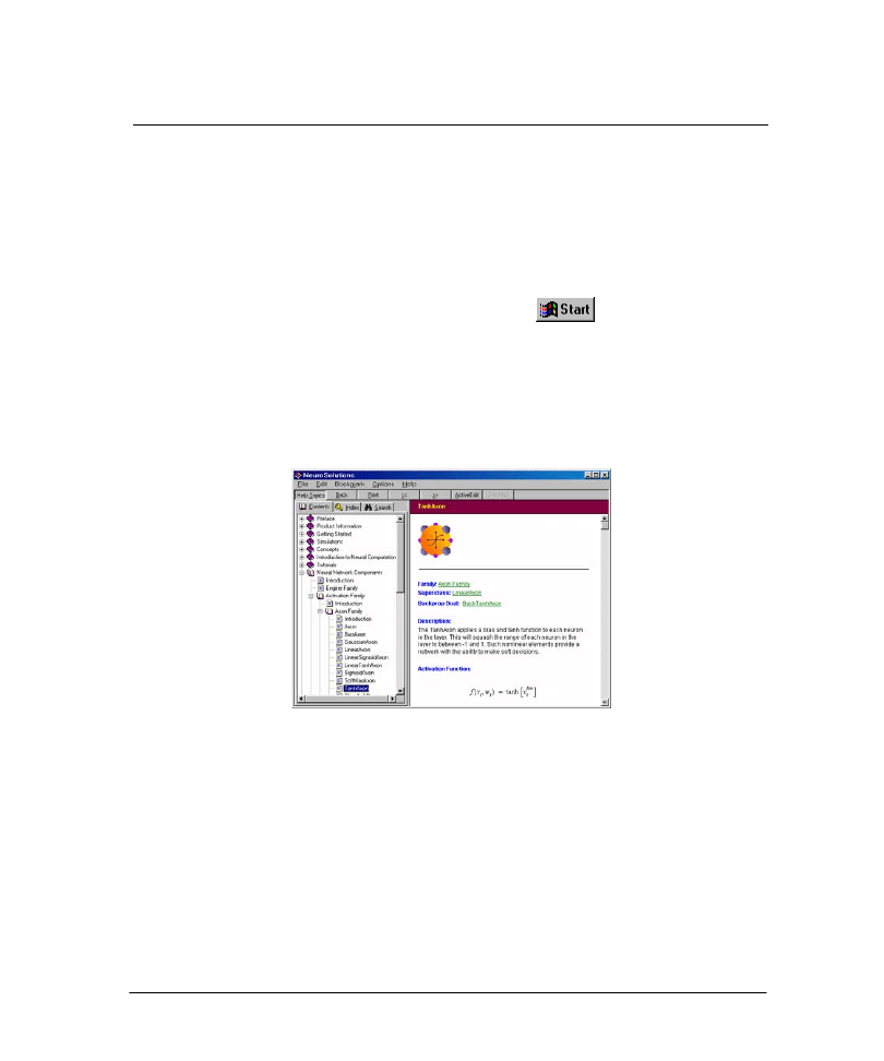
3.3 U
SING THE
O
NLINE
H
ELP
In addition to running the demos, the next best way to learn about NeuroSolutions is to
browse the online help. The online help is extensive, with several hundred topics
documenting all features of NeuroSolutions. It also has additional examples and tutorials,
as well as an introduction to neural networks.
Launching the Online Help
To launch the online help from the Windows Start Menu
:
Go to Start
⇒
NeuroSolutions 5
⇒
NeuroSolutions Help.
To launch the online help from within NeuroSolutions:
Go to the Help menu and select "NeuroSolutions Help" or press F1.
You may then get help by topic, index or keyword.
NeuroSolutions Help Topics
The Getting Started Manual is also available online. Simply launch it as you would the main
online help. This manual may be useful when you try the examples.
Context-Sensitive Help
NeuroSolutions also provides context-sensitive help. To access context-sensitive help:
Go to the Help menu and choose "Context Help" or press "Shift-F1".
Then click on any icon in the palettes, any component on the breadboard, or a property
page of the Inspector, and the help file will automatically open to the associated topic.

14
Printing the Online Help
From the main help topics page, you can print out the entire help file. To print out a
single chapter, open that chapter from the main help topics page and then print.
Alternatively, you can print out an individual topic from a topic page. The entire
documentation is also available in PDF format from the Download section of the
NeuroSolutions web site (
www.neurosolutions.com)
.
NeuroSolutions FAQ
Within the online help you will find a special section called the NeuroSolutions Frequently
Asked Questions (FAQ), a compendium of the most common questions received by
technical support. Beginning users may want to consult it before searching the general
help.

15
Chapter 4: B
UILDING A
N
EURAL
N
ETWORK
4.1 F
OUR
W
AYS TO
C
ONSTRUCT A
N
EURAL
N
ETWORK
There are four ways to build a neural network:
1. Run the NeuralExpert program.
2. Run the NeuralBuilder program.
3. Run a pre-recorded macro (such as one of the demos) and modify the resulting network.
4. Manually construct a network from a blank breadboard.
For the beginning user the easiest way to build a network is to use the NeuralExpert.
More advanced users who want more control of the topology and parameter settings may
want to use the NeuralBuilder. It is important to note that breadboards built with either
the NeuralExpert or NeuralBuilder can be modified later.
The NeuralExpert
The NeuralExpert asks you questions and intelligently builds a neural network. It
configures the parameters and probes based on your description of the problem to be
solved. Once you select a problem type you will see all the questions you will need to
answer in the panel on the left. You can click on these steps/numbers to navigate through
the question and answer session. Once the network is built, you can modify the settings
either directly on the breadboard or within the NeuralExpert.
NeuralExpert Opening Panel
16
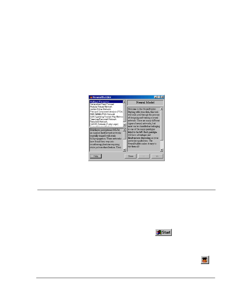
The NeuralBuilder
The NeuralBuilder is targeted for more advanced users. It presents a series of panels that
represent logical steps in the neural network design process. At each panel you make
choices and occasionally enter parameters. Instead of asking you questions based on the
problem type, as with the NeuralExpert, the NeuralBuilder allows you the specify the
neural network based on a particular neural model (topology).
Unlike the NeuralExpert, any modifications to the network must be made directly to the
breadboard – the NeuralBuilder does not have an edit capability. However, the
NeuralBuilder can be minimized and kept in the background, with all entered data still
intact. At any time, you can backtrack, make design changes, and then build another
network.
NeuralBuilder Opening Panel
4.2 T
HE
N
EURAL
E
XPERT
4.2.1 Starting the NeuralExpert
These following topics will take you through the various question panels of the
NeuralExpert. At each panel, the basic options will be explained, and suggestions offered.
You are encouraged to try the examples that are presented at the end of each panel’s
description. Each example continues throughout the chapter.
To launch the NeuralExpert from the Windows Start Menu
:
Select Start
⇒
NeuroSolutions 5
⇒
NeuralExpert
⇒
NeuralExpert.
To launch the NeuralExpert from within NeuroSolutions:
Go to the Tools menu and choose "NeuralExpert" or click the "NExpert" toolbar button
.
17
4.2.2 Getting Help in the NeuralExpert
Online help is available from all NeuralExpert panels. To access help for the current
panel, click the Help button in the lower left corner of the wizard.
NeuralExpert Help Topic for the Input File Specification Panel
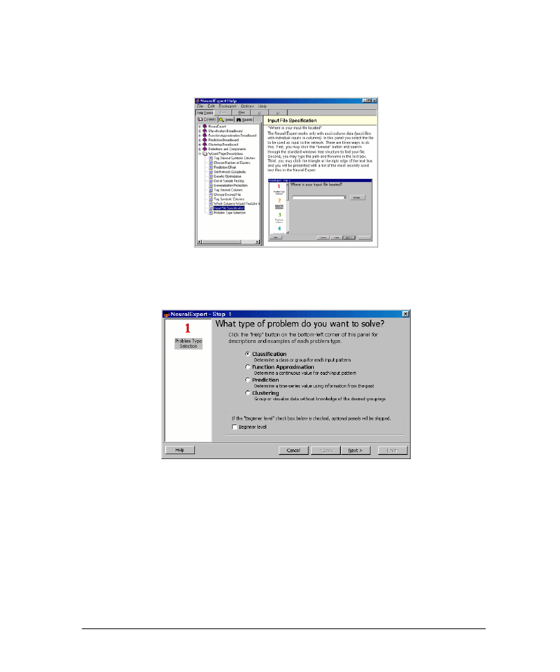
4.2.3 NeuralExpert Problem Type Selection Panel
NeuralExpert Problem Type Selection Panel
The first step in building a neural network with the NeuralExpert is the specification of
the problem type. The four currently available problem types in the NeuralExpert are
Classification, Prediction, Function Approximation, and Clustering. Please see the
NeuralExpert help file for detailed descriptions of these four problem types. If your
problem does not fit one of these descriptions (or you would like to completely specify
the architecture and parameters yourself), then you may want to use the NeuralBuilder
instead.
18
Example
9 Use the default "Classification" in the NeuralExpert Problem Type Selection panel.
9 For this example, uncheck the “Beginner level” switch so that we can examine some
of the advanced panels.
9 Click the Next button
to advance to the next panel.
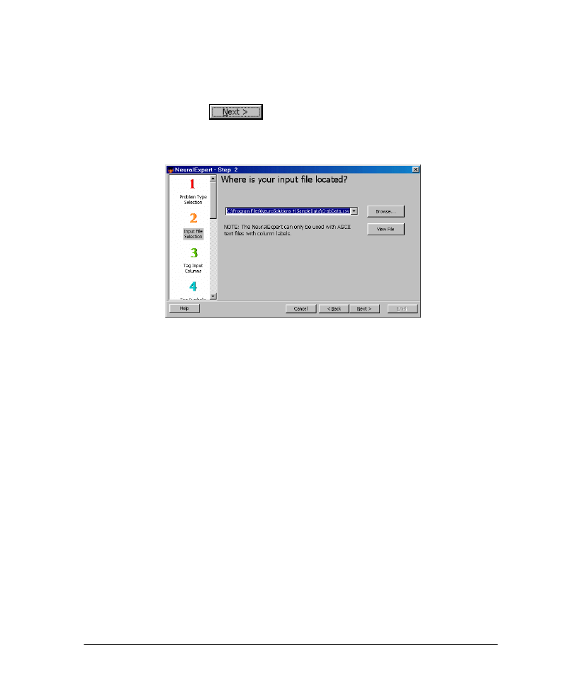
4.2.4 NeuralExpert Input File Selection Panel
NeuralExpert Input File Selection Panel
The next step in constructing your neural model is to select the input data. The
Input
File Selection
panel is where you specify where the input data file is located. There are
three ways to do this:
Click the "Browse" button and search through the standard windows tree structure to find your file.
Type the path and filename in the text box.
Click the triangle at the right edge of the text box and you will be presented with a list of the most
recently used text files in the NeuralExpert.
Please see the section on File Format Requirements before making this selection.
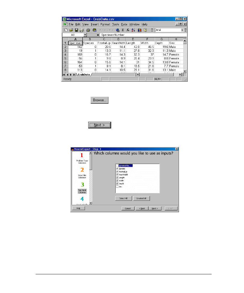
Example
The sample data we will use contain various attributes of stone crab specimens. There are
50 male and 50 female specimens for each of two species (blue form and orange form) for
a total of 200 specimens. The columns labeled "Species", "Frontal Lip", "Rear Width",
"Length", "Width", and "Depth" will serve as inputs to the neural network. The goal is to
train a neural network to determine the sex of a specimen (male or female) based on these
attributes.
19
Crab Classification Data used for the NeuralExpert Example
9 Click the Browse button
. The
Open
panel will display.
9 Navigate to the file "…\NeuroSolutions 5\SampleData\CrabData.csv" and double-
click it.
9 Click the View File button to view the file’s contents (optional).
9 Click the Next button
to advance to the next panel.
4.2.5 NeuralExpert Tag Input Columns Panel
NeuralExpert Tag Input Columns Panel
The next step in constructing your neural model is to tag the input columns. The
Tag
Input Columns
panel is where you specify which data you would like to feed into the
neural network. ASCII column data typically has column labels as the first row. If they do
not, the wizard will ask you if you would like to add column labels.
20
Example
The first column of this data is the specimen number, which is not useful information in
classifying the sex. The last column is the desired output ("Male" or "Female"). The rest of
the columns will be used as inputs to the network.
9 Uncheck the first item ("SpecimenNumber") and the last item ("Sex").
9 Click the Next button
to advance to the next panel.
9 All of the input columns have numeric data, so click the Next button
again to skip the Tag Symbolic Inputs panel.
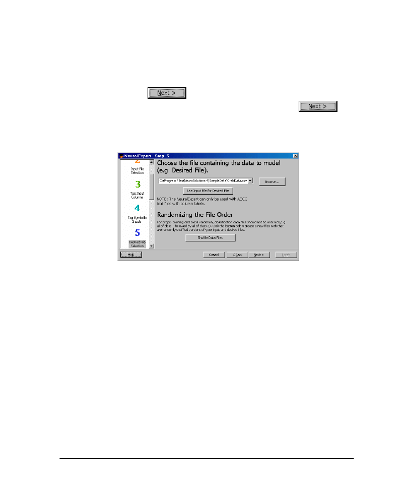
4.2.6 NeuralExpert Desired File Selection Panel
NeuralExpert Desired File Selection Panel
The next step in constructing your neural model is to select the desired output data. The
Desired File Selection
panel is where you specify where the desired output data file is
located. There are four ways to do this:
Click the "Browse" button and search through the standard windows tree structure to find your file.
Type the path and filename in the text box.
Click the triangle at the right edge of the text box and you will be presented with a list of the most
recently used text files in the NeuralExpert.
Click the "Use Input File as Desired File" button, which will place the input file name in the desired
file text box.
Please see the section on File Format Requirements before making this selection.
For classification problems you will be given the option to randomize the order of your
data before presenting it to the network. Neural networks train better if the presentation
of the data is not ordered. For instance, if you are classifying between two classes male
and female, the network will train much better if the male and female data are intermixed,
21
rather than all the males followed by all the females. If your data is highly ordered, you
should randomize the order before training the neural network.
Example
The file we chose for our input columns also contains the desired output column – the
sex of the specimen. The rows of this file are already randomized, so there is no need to
perform this operation again.
9 Click the Use Input File as Desired File button
. The path of the
input file should appear in the text box.
9 Click the Next button
to advance to the next panel.
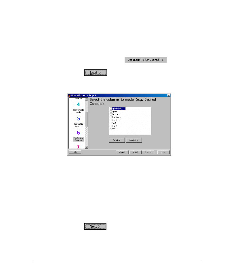
4.2.7 NeuralExpert Tag Desired Columns Panel
NeuralExpert Tag Desired Columns Panel
The next step in constructing your neural model is to tag the desired output columns. The
Tag Desired Columns
panel is where you specify which data you would like the neural
network to produce.
Example
The first column of this data is the specimen number, which is not something that we
want to try to classify. The next six columns have already been specified as the input data.
The last column is the desired output ("Sex").
9 Uncheck the first item ("SpecimenNumber"), but leave the last item ("Sex") checked.
9 Click the Next button
to advance to the next panel.
22
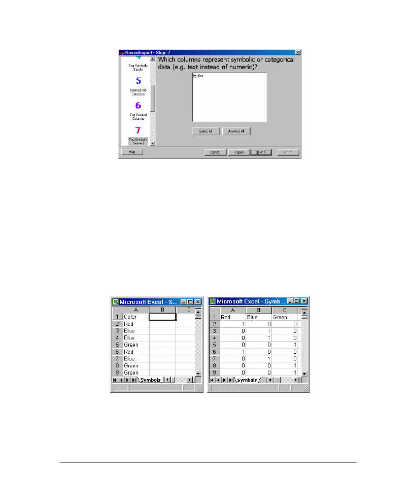
4.2.8 NeuralExpert Tag Symbolic Desired Panel
NeuralExpert Tag Symbolic Desired Panel
The
Tag Desired Columns
panel is used to specify which (if any) of the desired output
columns contain symbolic data. Symbolic columns are those in which each data element is
a string of characters (e.g. "yes"/"no"). Most often symbolic strings are non-numeric, but
columns containing discrete (non-continuous) numeric values should usually be tagged as
symbolic also.
NeuroSolutions translates a symbolic column by expanding it to N columns, where N is
the number of unique strings in the column. Each expanded column represents a
particular string. A "1" in an expanded column indicates the occurrence of the column’s
corresponding string and a "0" indicates a non-occurrence. The figure below illustrates a
symbolic column before and after the symbolic translation process.
Symbolic Column Before (left) and After (right) Symbolic Translation
23
Example
The desired output column contains non-numeric data – instances of "Male" or "Female"
specimens. Therefore, this column should be tagged as symbolic.
9 Leave the only item ("Sex") checked.
9 Click the Next button
to advance to the next panel.
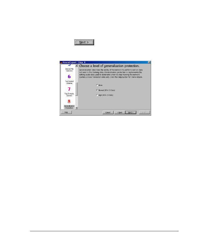
4.2.9 NeuralExpert Generalization Protection Panel
NeuralExpert Generalization Protection Panel
One of the primary goals in training neural networks is to ensure that the network
performs well on data that it has not been trained on (called "generalization"). The
standard method of ensuring good generalization is to divide your training data into
multiple data sets. The most common data sets are the training, cross validation, and
testing data sets.
The cross validation data set is used by the network during training. Periodically, while
training on the training data set, the network is tested for performance on the cross
validation set. During this testing, the weights are not trained, but the performance of the
network on the cross validation set is saved and compared to past values. If the network is
starting to overtrain on the training data, the cross validation performance will begin to
degrade. Thus, the cross validation data set is used to determine when the network has
been trained as well as possible without overtraining (i.e., maximum generalization).
The
Generalization Protection
panel is used to specify the amount of data to set aside
for cross validation. "None" indicates that all of the data in the input and desired files will
be used for training. This option is generally only used when you have very little data to
work with (e.g., less than 100 rows). "Normal" generalization protection specifies that
20% of your data will be set aside for cross validation. "High" generalization protection
will set aside 40% of your data for cross validation. This option should only be used when
you have a great deal of data (e.g. 10,000 rows or more).
24
Example
The data file for this example has 200 rows, so we will want to use "Normal"
generalization protection.
9 Check the "Normal" radio button.
9 Click the Next button
to advance to the next panel.
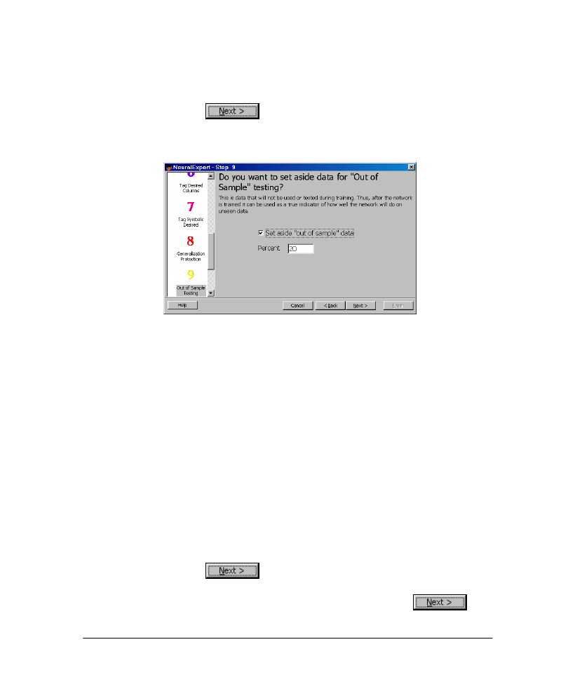
4.2.10 NeuralExpert Out Of Sample Testing Panel
NeuralExpert Out Of Sample Testing Panel
Although the network is not trained with the cross validation set, it uses the cross
validation set to choose a "best" set of weights. Therefore, it is not truly an out-of-sample
test of the network. For a true test of the performance of the network, an independent
(i.e., out of sample) testing set is used. This provides a true indication of how the network
will perform on new data.
The
Out Of Sample Testing
panel is used to specify the amount of data to set aside for
the testing set. The percentage will vary depending on the amount of data you have and
how rigorously you wish to test the network on out of sample data. The default value is
20% when this option is enabled.
Example
We would like to set aside 40 of the 200 rows of data to test the performance of the
network after training.
9 Check the "Set aside out of sample data" check box. Leave the "Percent" text box at
the default of 20.
9 Click the Next button
to advance to the next panel.
9 This problem is not complex enough to warrant the additional processing time
needed to perform parameter optimization, so click the Next button
again to skip the Genetic Optimization panel.
25
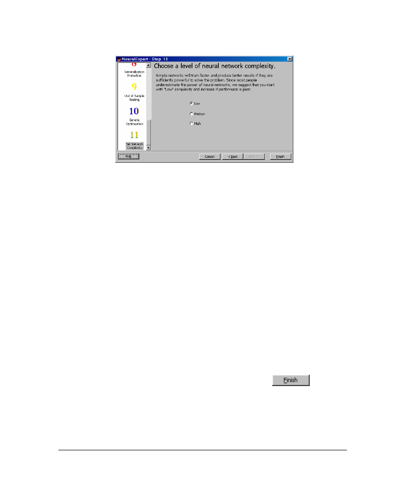
4.2.11 NeuralExpert Network Complexity Panel
NeuralExpert Network Complexity Panel
The
Network Complexity
panel is used to specify the size of the neural network in
terms of hidden layers and processing elements (neurons). In general, smaller neural
networks are preferable over large ones. If a small one can solve your problem sufficiently
(you would be surprised how powerful small networks are), then a large one will not only
require more training and testing time but also may perform worse on new data. This is
the generalization problem -- the larger the neural network, the more free parameters it
has to solve the problem. Excessive free parameters may over fit the data, causing the
network to overspecialize or memorize the training data. When this happens, the
performance of the training data will be much better than the performance of the cross
validation or testing data sets.
It is strongly recommended that you start with a "low complexity" network. After using a
low complexity network, you can move to a "medium" or "high" complexity network and
see if the performance is significantly better. Be warned that "medium" or "high"
complexity networks generally require a large amount of data (i.e., a thousand or more
training rows) to adequately train.
Example
We only have 120 rows of training data, so we should only need a low complexity
network.
9 Leave the default setting of "Low" and click the Finish button
to build
the neural network in NeuroSolutions.

26
NeuroSolutions Breadboard built with the NeuralExpert
After the network is built, a warning panel will be displayed indicating that there may not
be enough training data to adequately train the neural network. This is because this sample
data set has a small number of training exemplars (120) for the number of inputs we have
(6). This is not a problem since we are just using this data set for demonstration purposes.
If you get this panel when using a real data set and your network does not perform well
on the testing set, then you may need to either reduce the number of inputs or increase
the amount of training data.
27
Chapter 5: U
NDERSTANDING THE
B
READBOARD
5.1 B
READBOARD
I
CONS
Although you are no doubt anxious to try out your first simulation, a short digression on
understanding the NeuroSolutions breadboard is in order.
The Graphical User Interface and Simulations
NeuroSolutions adheres to the so-called local additive model. Under this model, each
component can activate and learn using only its own weights and the activations of its
neighbors. This lends itself very well to the object-oriented modeling, since each
component can be a separate object that sends and receives messages. This in turn allows
for a graphical user interface (GUI) with icon-based construction of networks.
When you see a group of components on the breadboard, it is important to understand
that it is much more than a picture; it is an actual representation of the underlying neural
network behind the user interface. What this means to the user is that there is a one-to-
one correspondence between the icons on the breadboard and the simulation that is going
on behind the GUI. Any network that you can construct on the breadboard can be
simulated. This is the key to the power of NeuroSolutions. In addition to all the standard
neural architectures, it is very easy to build and simulate novel architectures that are state
of the art in neurocomputing.
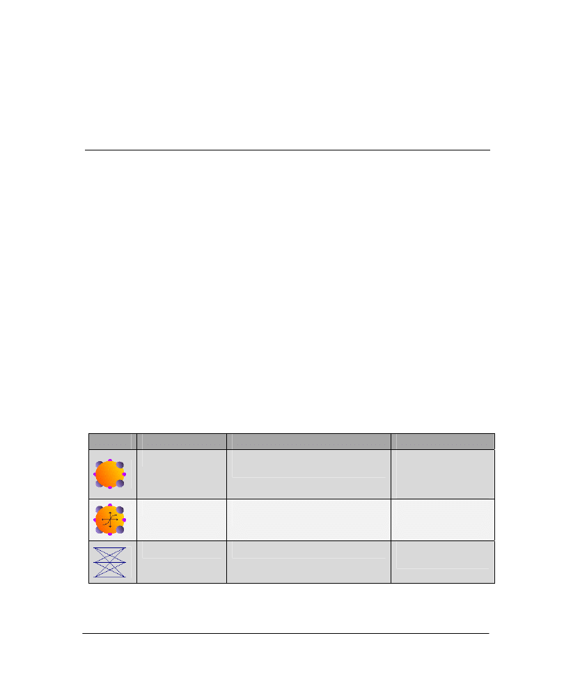
Here are some of the most common components:
Icon
Name
Description
Primary Usage
Axon
Layer of PE’s (processing elements) with
identity transfer function.
Can act as a placeholder
for the File component
at the input layer, or as a
linear output layer.
TanhAxon
Layer of PE’s with hyperbolic transfer
function (output range –1 to 1).
Used as hidden or
output layer.
FullSynapse
Full matrix multiplication.
Connects two axon
layers.
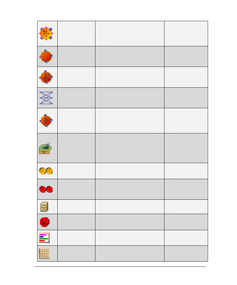
28
L2Criterion
Square error criterion.
Computes the error
between the output and
desired signal, and passes
it to the backpropagation
network.
BackAxon
Layer of PE’s with identity transfer
function.
Attaches to "dual"
forward Axon, for use in
backpropagation
network.
BackTanhAxon
Layer of PE’s with transfer function that
is the derivative of the TanhAxon.
Attaches to "dual"
forward TanhAxon, for
use in backpropagation
network.
BackFullSynapse
Back full matrix multiplication.
Attaches to "dual"
forward FullSynapse, for
use in backpropagation
network.
BackCriteriaControl
Input to backpropagation network.
Attaches to Criterion,
for use in
backpropagation
network. Receives error
from Criterion.
Momentum
Gradient search with momentum.
Updates weights.
Momentum increases
effective learning rate
when weight change is
consistently in the same
direction.
StaticControl
Static forward controller
Controls the forward
activation phase of
network.
BackStaticControl
Static backpropagation controller
Controls the backward
activation phase of
network
(backpropagation).
File
File input
For network input and
desired data from a file.
Threshold
Transmitter
Thresholded transmitter
For controlling one
component based on the
values of another.
BarChart
Bar chart probe
Displays data bar graph
style.
DataGraph
Graphing probe
Displays data versus
time.
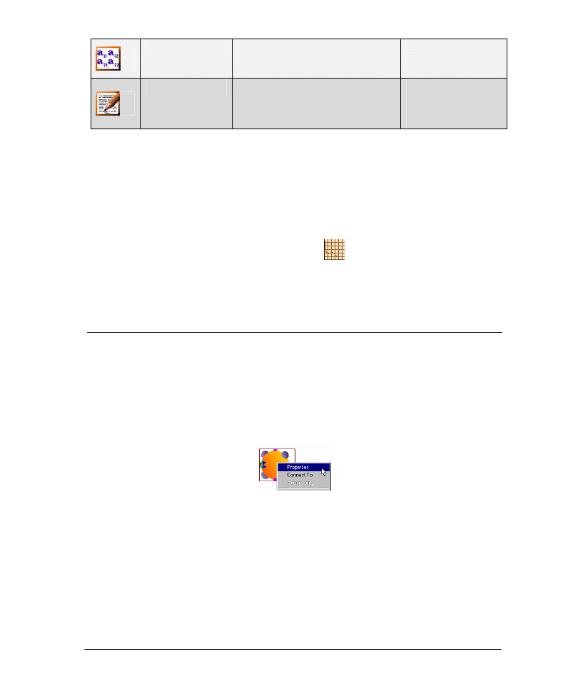
29
MatrixViewer
Numerical probe
Displays numerical
values at the current
instant in time.
DataWriter
Numerical probe
Displays numerical
values across time. Also
allows for the saving of
data to a file.
It is important to note that there may be probes stamped on the breadboard that are not
opened by default. The reason for this is that open probe display windows require
additional processing during training, which may slow down the simulation considerably.
However, you may find some of these probes to be useful, in which case you should open
them by double-clicking on the corresponding icon on the breadboard.
Example
9 Double-click on the top-most DataGraph icon
stacked on the right-most
TanhAxon (see table above). When the network is run, this probe has been set up to
display the network output vs. the desired output for the cross validation set.
5.2 T
HE
I
NSPECTOR
Every NeuroSolutions component also has a corresponding parameter set that you can
edit. You access a component’s parameter set though a dialog box called the Inspector.
Invoking the Inspector
You invoke the Inspector for any component on the breadboard by right-clicking its icon and choosing
"Properties"
Invoking the Inspector
You can also invoke the Inspector by left-click selecting an icon and then typing "Alt+Enter."
30
Sample Inspector
Property Pages
Once the Inspector is open, selecting any icon on the breadboard will change the
Inspector to reflect that component.
A component’s parameter set is organized according to property pages. The property
pages are labeled at the tabs across the top of the Inspector. You access the various
property pages by clicking on the tabs.
Simultaneously Editing Several Components
Thanks to NeuroSolutions’ object-oriented design, you will discover strong similarities
between the property pages of components within the same family. You can take
advantage of this by simultaneously editing the parameters of multiple components:
Invoke the Inspector for the first component.
Go to the property page of your choice.
Hold down the "Shift" key while left-click selecting the remaining components.
Edit any parameter(s) within the Inspector. Any changes you make in the Inspector will be reflected
in all selected components, so long as they all have the same parameter.
For example, you can simultaneously change the number of PE’s of a group of Axons,
even if they have different transfer functions (tanh, sigmoid, etc.).
Component Names
A name is one parameter that all components have in common. A component’s name can
be found on the Engine property page of its Inspector. Every component on a
breadboard must have a distinct name. The NeuralBuilder automatically named
components in a standard but intuitive fashion. For example, the Axon with a File
component is always named "inputAxon":
Example Component Name

31
You can name components any way you choose. However, most NeuroSolutions macros
supplied with the package expect that the components be named in a standard way. See
the online help topic "Naming" for more information.
32
Chapter 6: T
RAINING A
N
ETWORK
6.1 R
UNNING A
S
IMULATION
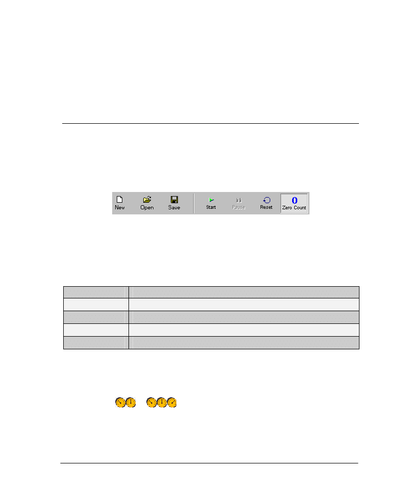
Default Toolbar
Once you have constructed a network, the next step is to train it. The basic network
controls are included in the default toolbar (called the Necessities toolbar), which contains
the following icons:
A segment of the NeuroSolutions Default Toolbar
If this toolbar is not visible, you can activate it by going to the Tools menu, choosing
"Customize", and checking the "Necessities" check box.
The following commands are most commonly used to control a simulation:
Name
Action
Start
Starts the simulation.
Pause
Pauses the simulation.
Reset
Resets the epoch and exemplar counters, and randomizes the weights.
Zero Counters
Resets the epoch and exemplar counters without randomizing the weights.
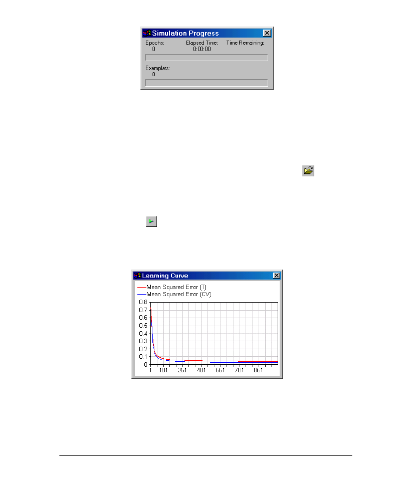
Monitoring a Simulation’s Progress
The Simulation Progress window provides a real-time graphic view of the number of epochs
that have been run. If this window is not visible, double-click the forward controller as
represented by
or
.
33
NeuroSolutions Simulation Progress Window
Example
This example picks up where the one from the previous chapter on the NeuralExpert left
off. Even if you did not follow the example in the previous chapter, you can still open an
existing breadboard that has been pre-saved for you:
9 Go to the File menu and select "Open," or type "Ctrl+O," or click the
toolbar
button.
9 Navigate to the file "…\NeuroSolutions\SampleData\CrabMLP.nsb" and double-
click it.
9 You are now ready to train the network.
9 Click the Start button
to begin the simulation to train the network. Note: this
button may be hidden behind a probe window.
The network will train for 1000 epochs. If the training was successful, the learning curves
should look something like this:
Sample Learning Curves
The red line corresponds to the error of the training set and the blue line corresponds the
error of the cross validation set. In most cases you will find that the cross validation error
will initially fall with the training error, but eventually will rise after the network begins to
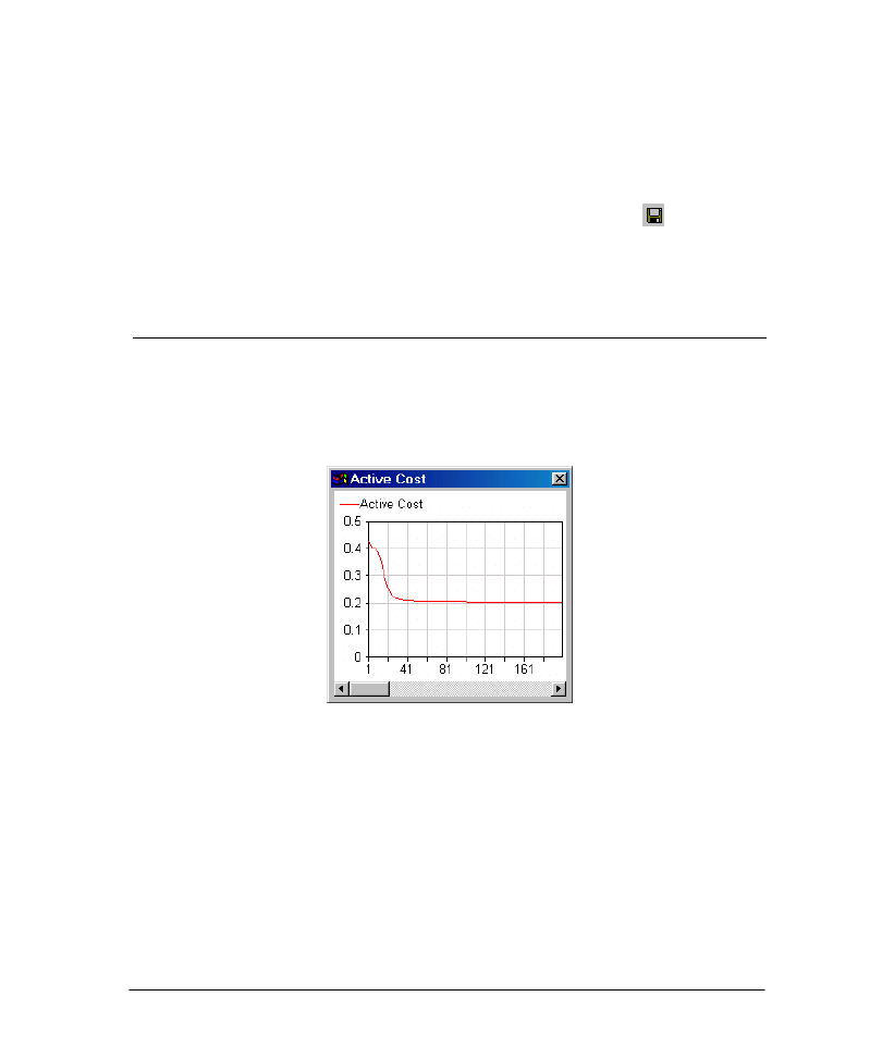
34
overtrain or "memorize" the data. The network is configured to automatically save the
weights of the network when the cross validation error reaches a bottom.
If your learning curves do not approach zero, then see the following section on
Recovering from an Unsuccessful Training for a discussion of possible reasons and
options.
It is always a good idea to save a breadboard after a successful training.
9 Go to the File menu and select "Save," or type "Ctrl+S," or click the
icon.
9 If you have not previously saved the breadboard, you will be prompted to save the
network with a name and location of your choice.
6.2 R
ECOVERING FROM AN
U
NSUCCESSFUL
T
RAINING
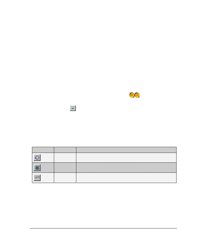
Identifying an Unsuccessful Training
It may happen that the network does not learn the problem. This is best evidenced by a
learning curve that does not approach zero.
An Unsuccessful Training
Three Possible Reasons for an Unsuccessful Training
If a training is unsuccessful, it is most likely due to one of three factors:
The network is capable of learning the problem but has not been trained long enough.
The network is capable of learning the problem but is stuck in a local minima.
The network is not powerful enough to learn the problem.
35
Increasing the Network’s Computing Power
If you have determined that the problem is not due to one of the first two possibilities,
then you will need to increase the number of processing elements in the network. If your
network was created with the NeuralExpert, you can increase the network’s computing
power by following these steps:
Click the "Modify" button on the breadboard.
Switch to the "Network Complexity" panel of the NeuralExpert (step #11 on the left side of the
panel).
If your network was "Low" change it to "Medium". If it was "Medium" change it to "High".
Click the "Finish" button to make the modifications to the network.
Increasing the Training Time
If the network has not been trained long enough, the simple remedy is to increase the
number of epochs and continue the training:
Invoke the Inspector for the forward controller by right clicking on
and selecting “Properties”.
On the
Static
property page, increase the "Epochs/Run."
Click the Start button
to continue the training.
Getting Out of a Local Minima
NeuroSolutions has several controls useful for getting a network out of a local minima.
These controls are available within the Control toolbar. If this toolbar is not visible, you
can activate it by going to the Tools menu, choosing "Customize", and checking the
"Control" check box.
Control
Name
Action
Reset
Resets the epoch and exemplar counters, and randomizes the weights.
Randomize
Randomizes the weights using Mean and Variance, specified on Soma
property page.
Jog
Randomizes the weights about their present values using the Variance,
specified on Soma property page.
If you are stuck in a local minima you may want to first try jogging the weights and
continuing the training. If that doesn’t work you may want to reset or randomize the
network and train again.
36
6.3 V
ERIFYING THE
T
RAINING
Although the mean square error is a good overall measure of whether a training run was
successful, sometimes it can be misleading. This is particularly true for classification
problems. When "Classification" is selected as the problem type, the NeuralExpert stamps
a pair of confusion matrix probes – one for the training set and one for the cross
validation set (assuming that you selected either "Normal" or "High" Generalization
Protection).
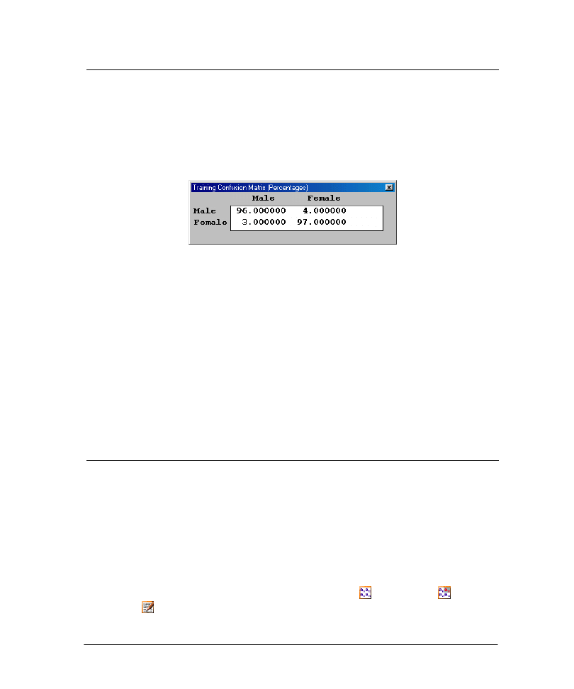
A Confusion Matrix Probe for the Training Set
The confusion matrix tallies the results of all exemplars of the last epoch and computes
the classification percentages for every output vs. desired combination. For example, in
the figure above, 96% of the male exemplars were correctly classified while 4% of the
male exemplars were classified incorrectly as female. Similarly, 97% of the female
exemplars were correctly classified while 3% of the female exemplars were classified as
male.
Example
9 Observe the "CrossVal" and "Training" confusion matrix probes displayed on the
breadboard to determine how well the training performed.
6.4 D
ENORMALIZING THE
P
ROBES
The NeuralBuilder and NeuralExpert automatically set up normalization of the input and
desired files. Normalization, the process of scaling and shifting the data to better match
the network’s range, is an important part of neural network pre-processing, and can
significantly speed up training.
Viewing the Data in its Native Range
When probing a network, however, it may be preferable to view the data in its original
range. This process is called denormalization. All probes that display the data numerically
are capable of denormalization, including the MatrixViewer , MatrixEditor , and
DataWriter . Access to this feature is from the Probes property page of the Inspector:
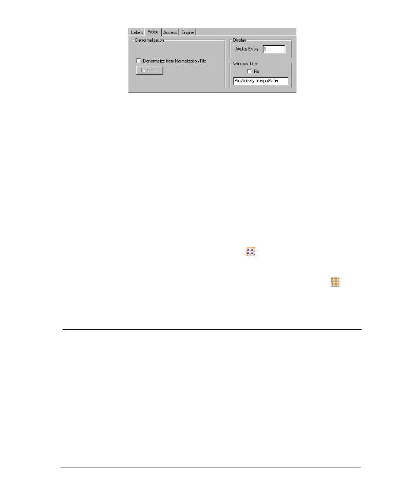
37
Probe Denormalization in the Inspector
Automatic Matching of Probe with Normalization File
Every data set generates its own normalization file, which stores the scale and offset of
the data. Probes can then use this normalization file to perform the denormalization. If
the probe is at the input File, NeuroSolutions will automatically choose the input File’s
normalization file to perform the denormalization. If the Probe is at either the output
Axon or desired File, the desired File’s normalization file will be used.
Note that denormalizing the probes does not in any way affect the training of the
network.
Example
By default the NeuralBuilder and NeuralExpert configure the probes on the breadboard
to display in the original data’s range. Let's verify that this setting is correct.
9 Invoke the Inspector for the bottom MatrixViewer on the desired File, and go to
the Probes property page.
9 Verify that the box "Denormalize from Normalization File" is checked
9 Repeat for the other desired MatrixViewer probe and the DataGraph probes
attached to the right-most TanhAxon.
6.5 M
ANUALLY
O
PTIMIZING THE
N
ETWORK
As mentioned previously, it is important to find the network with the minimal number of
free weights that can still learn the problem. The minimal network is more likely to
generalize well to new data. Therefore, once you have achieved a successful training, you
should then begin the process of decreasing the size of the network and repeating the
training until it no longer learns the problem to your satisfaction.
Note that NeuroSolutions does include a facility for optimizing various network
parameters using a genetic algorithm, but this topic is too advanced for this manual.
Interested users should refer to the NeuroSolutions, NeuralBuilder and/or NeuralExpert
documentation for detailed information on genetic optimization within NeuroSolutions.
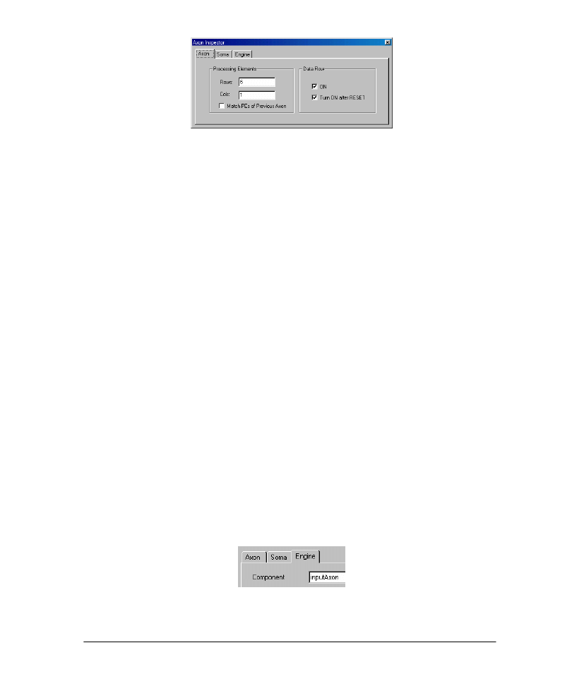
38
Example
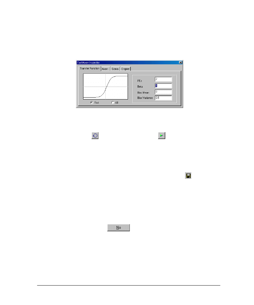
The NeuralExpert built the neural network with 3 PE’s on the hidden layer TanhAxon,
and the network learned the problem easily. Now we will decrease that number:
9 Invoke the Inspector for the hidden layer TanhAxon.
9 Enter "2" in the edit box for the number of Rows.
TanhAxon Inspector After Changing the Number of PE’s to 2
Now we will re-train the network:
9 Click the Reset button
, followed by the Start button
.
9 Observe the learning curve and confusion matrices to see whether the network
learned the problem.
If the network did not learn, re-train several more times to make sure the network was not
stuck in a local minima. You should find that this size network can learn the problem.
Once the network learns the problem, save the breadboard:
9 Go to the File menu and select "Save," or type "Ctrl+S," or click the
icon.
9 Let’s now decrease the number of Rows to 1:
9 Enter "1" in the edit box for the number of PE’s.
9 Repeat the training process as previously described.
You may observe that the network does not solve the problem as well with 1 PE. If this is
the case, you can conclude that 2 PE’s on the hidden layer is optimal. To load in the
breadboard trained with 2 PE’s:
9 Go to the File menu and choose "Close."
9 When prompted, select "No"
to saving the breadboard.
9 Go to the File menu and choose the most recent file name you used from the list at
the bottom of the menu.
39
Chapter 7: T
ESTING A
N
ETWORK
7.1 S
TARTING THE
T
ESTING
W
IZARD
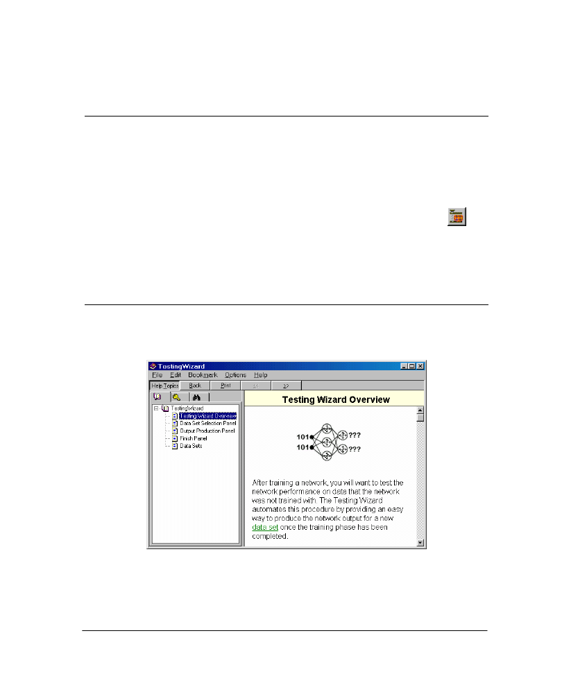
After training a network, you will want to test the network performance on data that the
network was not trained with. The TestingWizard automates this procedure by providing
an easy way to produce the network output for the testing dataset that you defined within
the NeuralExpert or NeuralBuilder, or on a new dataset not yet defined.
To launch the TestingWizard from within NeuroSolutions:
Go to the Tools menu and choose "TestingWizard" or click the "Testing" toolbar button
.
If your breadboard was built with the NeuralExpert, you may alternatively:
Click the "Test" button in the upper-left corner of the breadboard.
7.2 G
ETTING
H
ELP IN THE
T
ESTING
W
IZARD
Online help is available from all TestingWizard panels. To access help, click the Help
button in the lower left corner of the wizard.
TestingWizard Help Window
40
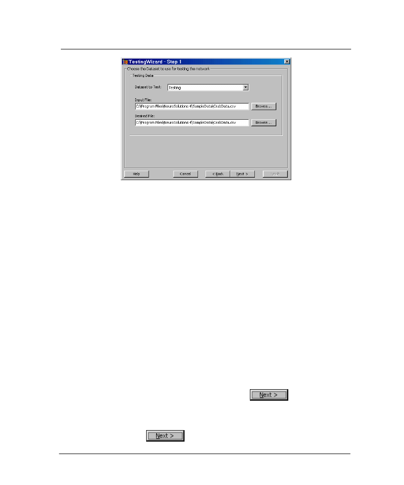
7.3 T
ESTING
W
IZARD
D
ATA
S
ET
S
ELECTION
P
ANEL
TestingWizard Data Set Selection Panel
This panel is used to specify the data to use for your test. The two most common data sets
to use are Testing and Production. Testing is used if there is desired data that corresponds
to the input data. Production is used if you do not know what the output is supposed to
be – you want to neural network to tell you. You may also test the network using the
Training or Cross Validation sets.
If the selected data set has already been defined, either manually or using one of the
wizards, then the file path(s) will be filled in for you by default. If you have not yet defined
the data set, or would like to override the existing file settings, click the Browse button(s)
to define the input and/or desired files.
Note that the input file for the Testing/Production set must have the same column labels
as the input file used for the training set. Likewise, the desired file of the Testing set must
be of the same structure as the training desired file.
Example
Recall that within the NeuralExpert we had allocated 20% of the data file for the testing
set. The TestingWizard detects this automatically, so there is no need to specify the files
again.
9 Launch the TestingWizard.
9 Read the Introduction panel and click the Next button
to advance to the
file selection panel.
9 Note that the data set defaults to Testing and the input and desired file paths are
already filled in.
9 Click the Next button
to advance to the next panel.
41
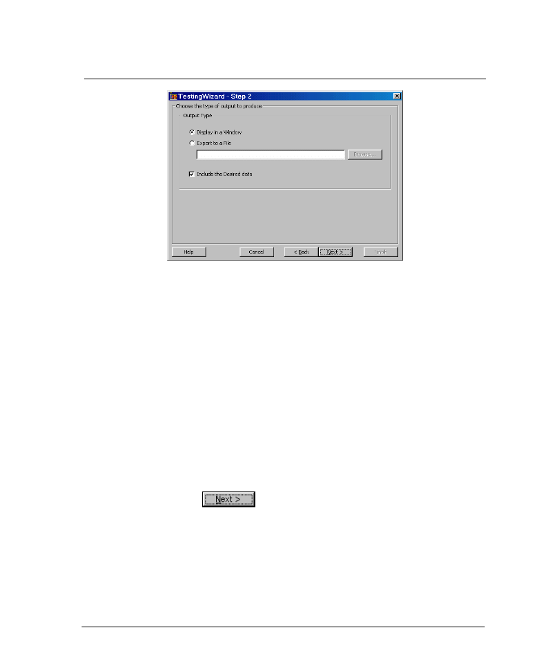
7.4 T
ESTING
W
IZARD
O
UTPUT
P
RODUCTION
P
ANEL
TestingWizard Output Production Panel
This panel is used to specify how the network output of the testing set should be
produced. The DataWriter probe is the component used to extract the output data. You
may either display the output data in a window or have the data written to an ASCII file.
To do this, click the "Export to a file" radio button, click the "Browse" button and specify
a file name and directory to write the output data to.
You may also include the desired data within the display/file in order to do a side-by-side
comparison. If you only want to produce the output data, uncheck the "Include the
Desired Data" box.
Example
We will keep the default settings, which will produce the testing results within a display
window and include the desired response with the network output.
9 Make sure that the "Display in a Window" radio button is selected and the "Include
the Desired Data" checkbox is checked.
9 Click the Next button
to advance to the next panel.
9 Click the Finish button to test the network.
9 Observe the results by scrolling through the window labeled "Desired and Output".
42
Chapter 8: T
HE
N
EURAL
B
UILDER
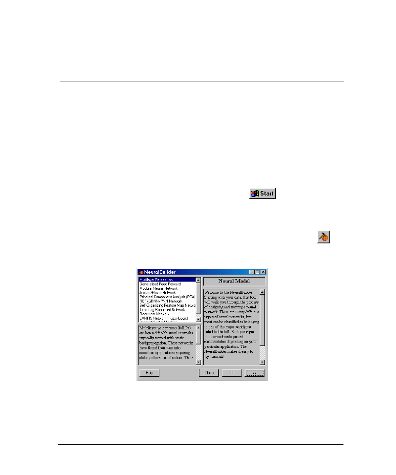
8.1 S
TARTING THE
N
EURAL
B
UILDER
An alternative to the NeuralExpert is the NeuralBuilder. This neural network construction
utility provides more flexibility in specifying the neural network topology and parameters.
In the following topics, we will take you through the various design panels of the
NeuralBuilder. At each panel, the basic design options will be explained, and suggestions
offered. If you would like to understand the rationale behind some of the suggestions,
please see the section on Neural Network Training Hints.
We encourage you try the examples that are presented at the end of each panel’s
description. Each example continues throughout this chapter. For this reason, we
recommend you do not skip any panels.
To launch the NeuralBuilder from the Windows Start Menu
:
Select Start
⇒
NeuroSolutions 5
⇒
NeuralBuilder.
To launch the NeuralBuilder from within NeuroSolutions:
Go to the Tools menu and choose "NeuralBuilder" or click the "NBuilder" toolbar button
.
The following panel will appear:
NeuralBuilder Neural Model Panel
43
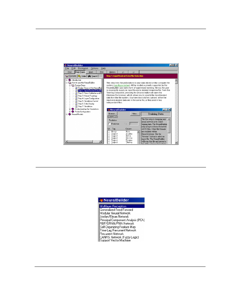
8.2 G
ETTING
H
ELP IN THE
N
EURAL
B
UILDER
Online help is available from all NeuralBuilder panels. To access help for the current
panel, click the Help button in the lower left corner of the wizard. Note that all other
topics of the help file can be accessed through the table of contents on the left side of the
help window.
NeuralBuilder Help Window
8.3 N
EURAL
B
UILDER
S
UPPORTED
M
ODELS
The first step in building a neural network is choosing a neural model. The NeuralBuilder
supports eleven neural models, shown below. For a complete description of these models,
and how to choose one for your application, see Choosing a Neural Architecture.
NeuralBuilder Supported Models
44
The Multilayer Perceptron is by far the most common neural network model. We will use
it as the basis of our example as we take you through the various NeuralBuilder panels.
Now, to get started …
Example
9 Use the default "Multilayer Perceptron" in the NeuralBuilder
Neural Model
panel.
9 Click the Forward button
to advance to the next panel.
8.4 N
EURAL
B
UILDER
T
RAINING
D
ATA
P
ANEL
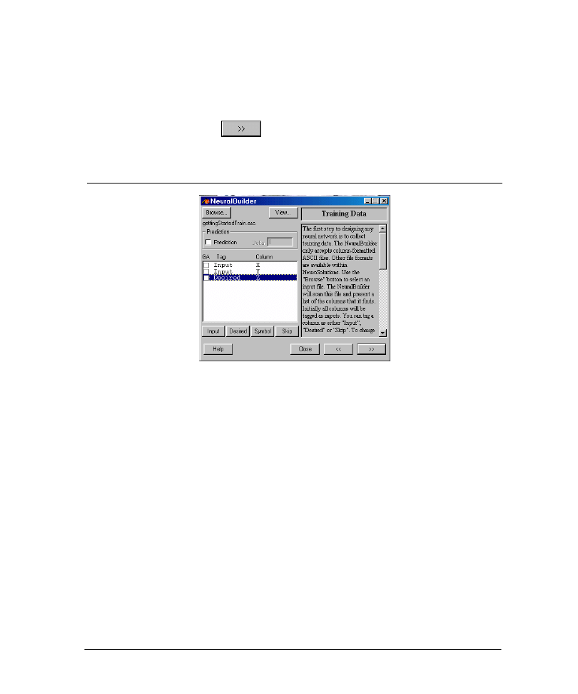
NeuralBuilder Training Data Panel
The next step in constructing your neural model is to select the training data. The
Training Data
panel is where you:
Choose your file.
Tag the columns according to usage.
For time series only, specify that the goal of the training is prediction, where "Delta" is the number of
time steps in the future to predict.
Please see the section on File Format Requirements before making the file selection.
Tagging Columns
By default, all columns are tagged as "Input." You can change the default setting of any
column to the "Desired" response of the network, specify that the column contains
"Symbols" that need to be converted to numeric data, or "Skip" the column entirely.
The "GA" checkboxes are used to indicate that a genetic algorithm is to determine if the
corresponding input is to be included or skipped. Genetic Algorithms are general-purpose
search algorithms based upon the principles of evolution observed in nature. Genetic
algorithms combine selection, crossover, and mutation operators with the goal of finding
45
the best solution to a problem. They search for this optimal solution until a specified
termination criterion is met. In NeuroSolutions the criteria used to evaluate the fitness of
each potential solution is the lowest cost achieved during the training run. Please see the
documentation for NeuroSolutions and the NeuralBuilder for more information on this
topic.
Training and Desired Files
The input and desired data can be either in the same file, or split into separate files. If they
are in separate files, and you do not tag any columns as "Input" in this panel, then the
Desired Response
panel will immediately follow this panel, where you can specify the
separate desired file.
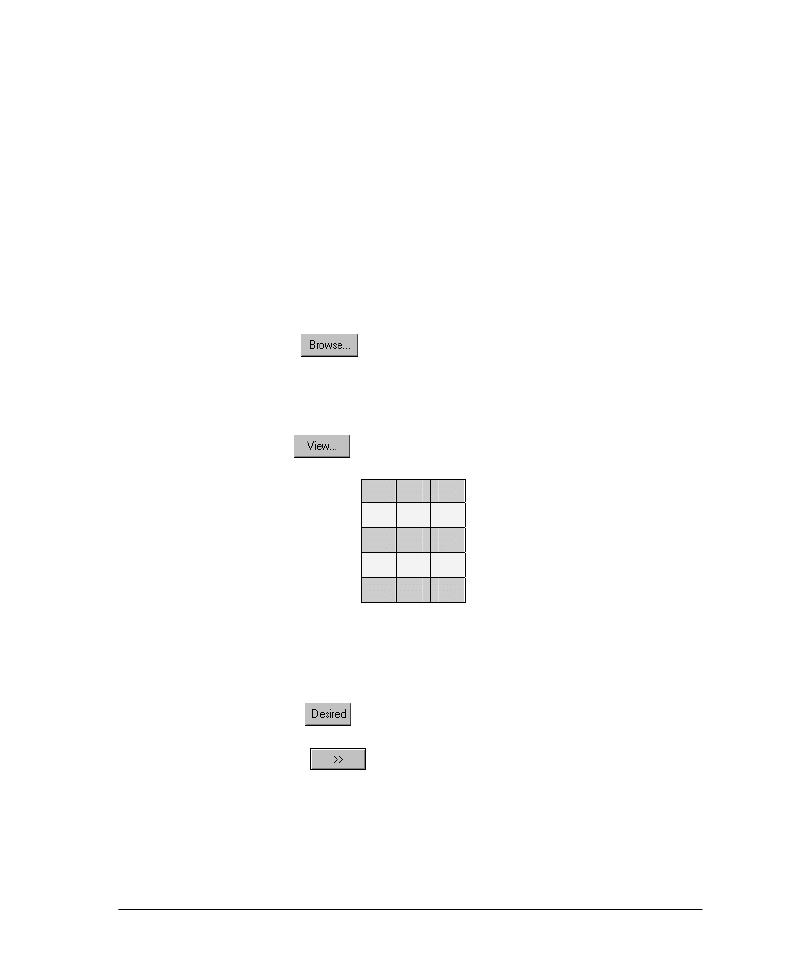
Example
Our example contains both input and desired data in the same file:
9 Click the Browse button
. The
Open
panel will display.
9 Navigate to the file "…\NeuroSolutions 5\SampleData\gettingStartedTrain.asc" and
double-click it.
9 Back in the
Training Data
panel, you should see a list of all the columns in the file.
Note that they are all initially tagged as Input.
9 Click the View button
to view the file’s contents:
X
Y
Z
0
0
0
0
1
1
1
0
1
1
1
0
This data is the input-output response of an exclusive-or logic gate. The X and Y columns
are the voltage inputs to the gate, and the Z column is the expected output of the gate,
given the inputs. There are a total of four exemplars. To tag column Z as the desired data:
9 Select column "Z."
9 Click the Desired button
. You should see the "Z" column tag change from
"Input" to "Desired":
9 Click the Forward button
to advance to the next panel.
46
8.5 C
ROSS
V
ALIDATION AND
T
EST
D
ATA
P
ANEL
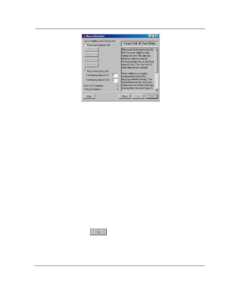
NeuralBuilder Cross Validation and Test Data Panel
This panel is used to specify the cross validation and/or testing data sets. These data sets
can be specified as a percentage of the exemplars from the training file, or they can be
input from separate files.
Cross Validation Set
Neural networks can be overtrained to the point where performance on new data actually
deteriorates. Roughly speaking, overtraining results in a network that memorizes the
individual exemplars, rather than trends in the data set as a whole. Cross validation is a
process whereby part of the data set is set aside for the purpose of monitoring the training
process, to guard against overtraining.
Testing Set
The testing set is used to test the performance of the network. Once the network has been
trained, the weights are then frozen, the testing set is fed into the network, and the
network output is compared with the desired output.
Example
Because we are working with a small data set, we will not specify a cross validation or
testing set.
9 Click the Forward button
to advance to the next panel.
47
8.6 N
EURAL
B
UILDER
T
OPOLOGY
P
ANEL
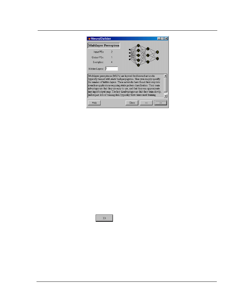
NeuralBuilder Multilayer Perceptron Panel
The Topology
panel is specific to the neural model chosen in the first panel. This is
where you set:
The number of hidden layers, and
Parameters specific to the architecture you chose in the first panel.
Number of Hidden Layers
Common to all models is a text box for the number of hidden layers. Unless you believe
your problem is particularly difficult, start with the default setting of one hidden layer; you
can always return later and add additional layers.
Example
For the Multilayer Perceptron, the number of hidden layers is the only parameter in this
panel. One hidden layer should be sufficient to solve the exclusive-or problem.
9 Use the default value of "1" as the number of Hidden Layers.
9 Click the Forward button
to advance to the next panel.
48
8.7 N
EURAL
B
UILDER
H
IDDEN
L
AYER
P
ANEL
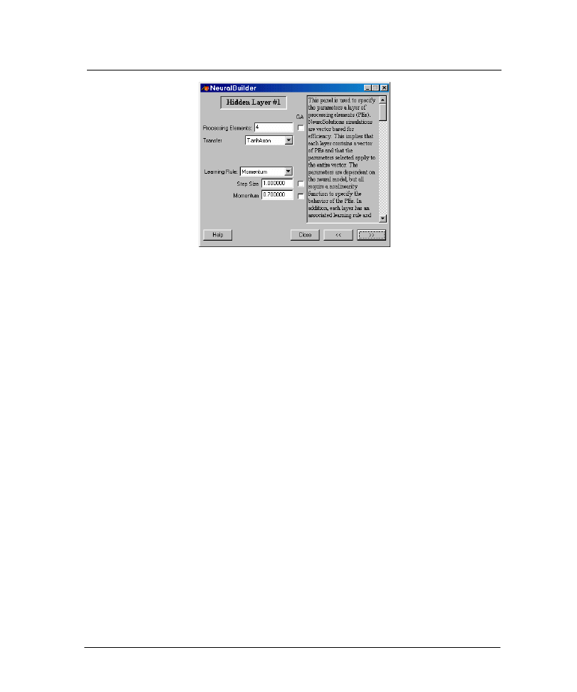
NeuralBuilder Hidden Layer #1 Panel
The
Hidden Layer
panel is where you choose:
The number of processing elements in the layer.
The layer’s transfer function.
The layer’s learning rule and parameters.
For each number of hidden layers requested in the Topology
panel, separate
Hidden
Layer
panels will appear in sequence.
Number of Processing Elements
The most important parameter you need to set here is the number of processing elements
(PE’s). The number of PE’s directly affects the overall computing power of the network.
Ideally, the number of PE’s should be chosen based on the complexity of the desired
input-output mapping of the data, but really can only be determined experimentally.
It is important to note that the minimal number of PE’s needed to solve a problem need
not be related to the size of the data set. However, the NeuralBuilder does not know the
complexity of the data, and thus chooses the number of PE’s proportional to the number
of input channels. This is likely to overestimate the required number of PE’s, but at least
the network is likely to learn on the first trial. However, good generalization to new data
depends on finding the minimal number of PE’s that can solve the problem.
The "GA" checkbox next to the "Processing Elements" text box is used to indicate that a
genetic algorithm will be used to determine the number of processing elements that
produced the lowest cross validation error during a large number of training runs. Genetic
optimization is beyond the scope of this manual. Please see the documentation for
NeuroSolutions and the NeuralBuilder for more information on this topic.

49
Transfer Function
It is the non-linearity of the hidden layer’s axons that give a neural network the
computational ability to learn difficult problems. Of the eight axons offered by the
NeuralBuilder,
Axon
Output Range
Features
TanhAxon
-1 to 1
Nonlinear axon of choice.
SigmoidAxon
0 to 1
Same general shape as TanhAxon.
LinearTanhAxon
-1 to 1
Piecewise linear approximation to TanhAxon.
LinearSigmoidAxon
0 to 1
Piecewise linear approximation to SigmoidAxon.
SoftMaxAxon
0 to 1
Outputs sum to 1. Used for classification.
BiasAxon
Infinite
Linear axon with adjustable slope and adaptable bias.
LinearAxon
Infinite
Linear axon with adaptable bias.
Axon
Infinite
Simplest axon, identity transfer function.
only the first five are non-linear. Of those five, only the TanhAxon and SigmoidAxon are
commonly used on the hidden layer(s).
For most problems, use the recommended TanhAxon transfer function.
Input File Normalization
The NeuralBuilder will automatically instruct NeuroSolutions to scale and shift the input
data to match the range of the first hidden layer’s transfer function. For example, if the
first hidden layer’s axon is a TanhAxon, the input data will be scaled and shifted to lie
between –1 and 1. This important pre-processing step is called normalization, which will
be discussed later.
Learning Rules
The learning rule, also called gradient search, is used to calculate the weight update.
NeuroSolutions and the NeuralBuilder offer five learning rules:
NeuralBuilder Learning Rules
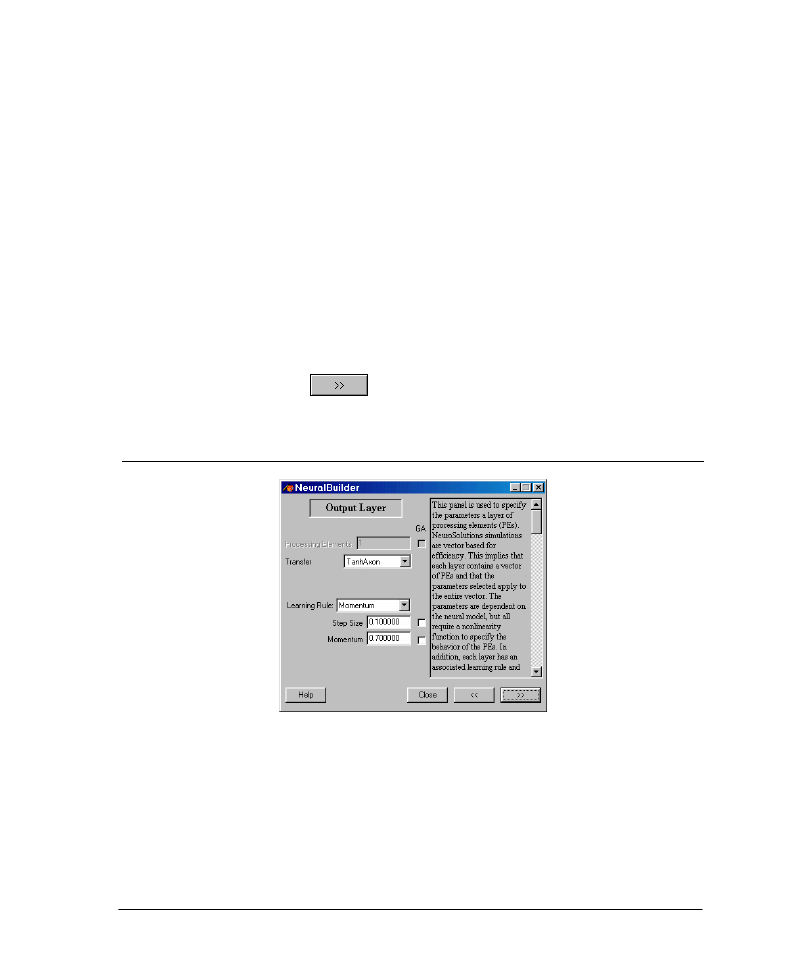
50
Beginning users should use Momentum learning for all layers. Though not potentially as
fast as Quickprop, DeltaBarDelta or ConjugateGradient, Momentum learning is generally
more stable.
It is usually quite safe to go with the recommended values for the learning parameters.
The "GA" checkboxes next to the learning parameters are used to indicate that a genetic
algorithm will be used to determine the parameters. Genetic optimization is beyond the
scope of this manual. Please see the documentation for NeuroSolutions and the
NeuralBuilder for more information on this topic.
Example
Although non-linear, the exclusive-or problem is not particularly difficult. Therefore, we
will start out with 3 processing elements:
9 Enter "3" into the Processing Elements edit box.
9 Use the default "TanhAxon" as the layer’s PE Transfer function.
9 Use the default "Momentum" as the Learning Rule, along with the default "0.1" Step
Size and "0.7" Momentum.
9 Click the Forward button
to advance to the next panel.
8.8 N
EURAL
B
UILDER
O
UTPUT
L
AYER
P
ANEL
NeuralBuilder Output Layer Panel
This panel is identical to the panel for the hidden layer(s), except that the number of
Processing Elements is completely determined by the number of channels of desired
response data.
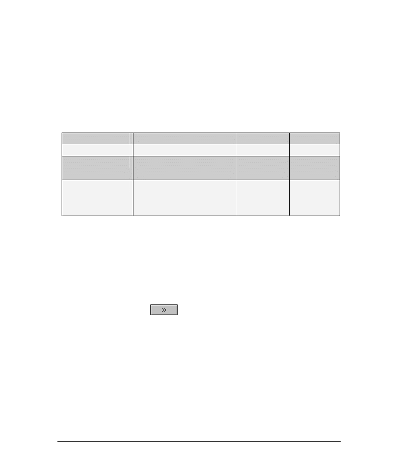
51
Output File Normalization
Just as for the input data, the NeuralBuilder will automatically normalize the desired
response data to match the range of the output transfer function. For example, if the
output layer is a TanhAxon, the desired response data will be normalized to lie between –
1 and 1.
Transfer Function
It is important to choose the output layer’s transfer function to match the problem. Use
the following table as a guide to choosing the proper output Axon:
Problem
Description
Output Range
Output Axon
Multi-way classification
1 of N classification.
0 to 1
SoftMaxAxon
Two-way classification
1 of 2 classification, with only a single
desired channel.
-1 to 1or 0 to 1
TanhAxon or
Sigmoid
Regression
Desired response is a continuous
function of the input.
Infinite
Axon
BiasAxon
LinearAxon
Again, it is usually quite safe to stick with the recommended values for the learning
parameters.
Example
The exclusive-or problem has only a single channel of desired response, and therefore the
number of PE’s chosen by the NeuralBuilder is 1. We will choose the TanhAxon as the
output layer transfer function.
9 Use the default "TanhAxon" for the output layer PE Transfer function.
9 Click the Forward button
to advance to the next panel.
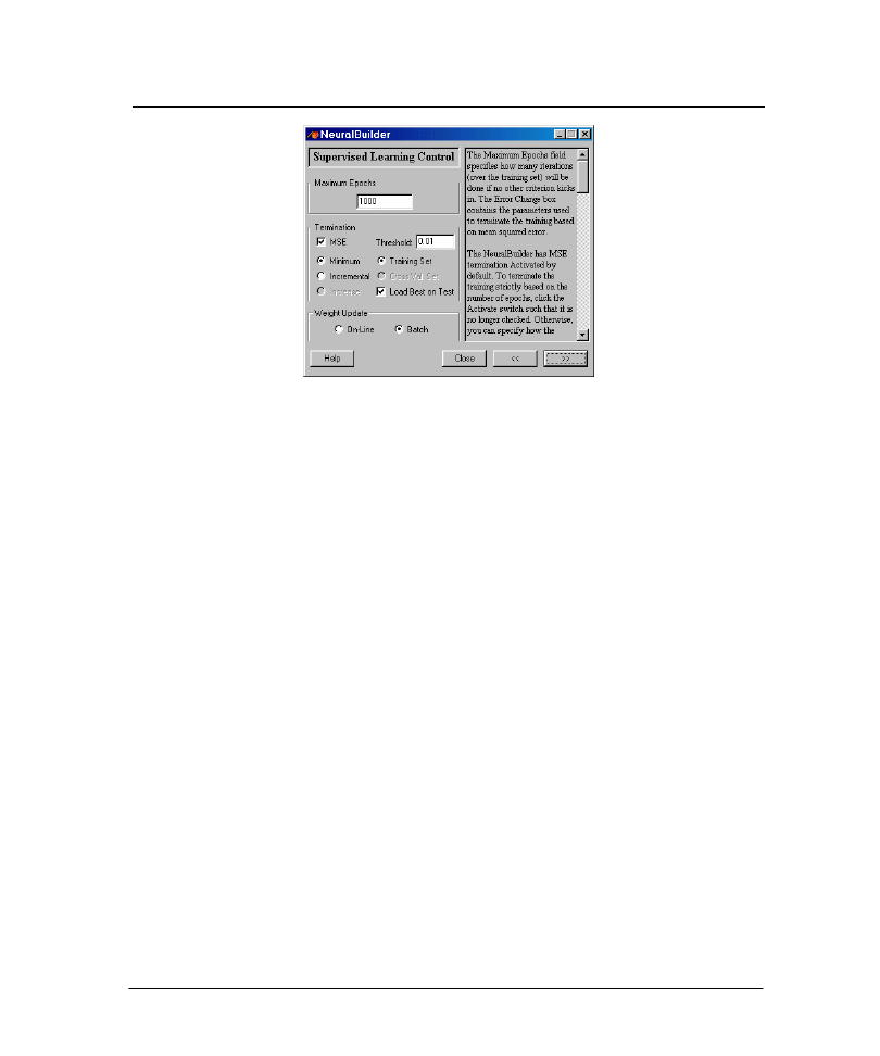
52
8.9 N
EURAL
B
UILDER
S
UPERVISED
L
EARNING
P
ANEL
NeuralBuilder Supervised Learning Panel
The
Supervised Learning
panel is where you:
Enter the
Maximum Epochs
to train.
Specify
Termination
criteria for stopping the training.
Choose the frequency of
Weight Update
.
Maximum Epochs
Many problems should be learnable within the default 1000 epochs; thus the default is a
reasonable starting point.
Termination Criteria
The Termination criteria, when "MSE" (mean square error) and "Minimum" are chosen,
sets up the necessary breadboard components so that the training stops when the error
reaches the "Threshold." Stopping the learning in this fashion keeps the network from
overtraining, and thus is particularly desirable if cross validation is not being used. The
default "Threshold" is usually adequate.
When cross validation is used, the default configuration is to have the training stop when
the cross validation error begins to increase. The best weights of the network are
automatically saved at the point when the cross validation error is at its lowest point.
When testing the network, these best weights are loaded into the network before the
testing data is fed through the network (if the "Load Best on Test" switch is set).
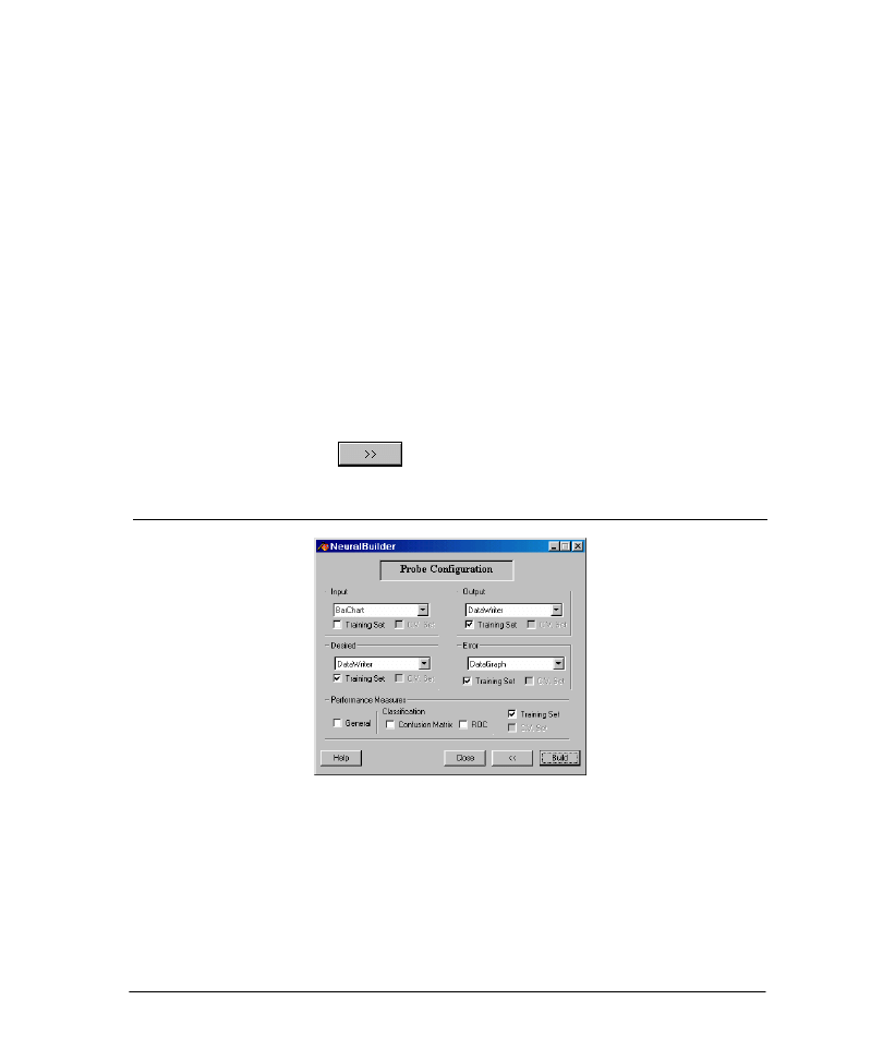
53
Weight Update
The Weight Update option determines when the network weights are updated. "Online"
learning updates the weights after the presentation of each exemplar, while "Batch"
learning waits until the entire training set has been presented, and thus effectively averages
the weight updates over the data set. For beginning users, we recommend "Batch" weight
update because the learning is stable over a wider range of step sizes. However, for large
data sets, the "Online" weight update can be significantly faster, although it requires a
more careful tuning of the learning parameters.
Example
The exclusive-or problem is not particularly difficult, therefore we will stop the training
after 200 epochs maximum. However, we do not want to overtrain, so we will use a
Termination criterion.
9 Enter "200" as the Maximum Epochs.
9 Use the defaults "MSE" and "Minimum" as the Termination criteria, and "0.01" as the
Threshold.
9 Use the default "Batch" as the Weight Update.
9 Click the Forward button
to advance to the next panel.
8.10 N
EURAL
B
UILDER
P
ROBE
C
ONFIGURATION
P
ANEL
NeuralBuilder Probe Configuration Panel
NeuroSolutions can probe the data flowing through a network, or any of its parameters,
using a variety of visualization tools. The NeuralBuilder concentrates on the most
important of these. In the
Probe Configuration
panel, you can:
Choose the type of probe for any of the following points in the network, such as
Input
,
Output
,
Desired
response,
Error
or
Weights
.
Monitor the performance of the network during training.
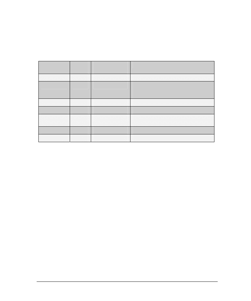
54
Specify whether the probes will monitor training, cross validation, or both.
Build the network.
Probe Types
NeuroSolutions offers many different probes. The NeuralBuilder handles the seven most
important probes, shown in the chart below:
Probe
Matrix
Style?
Accumulates
Data Over Time?
Feature
BarChart
No
No
Length of bar is proportional to value.
DataWriter
Yes
Yes
Accumulates the data over time in a separate
window, which can be saved as a text file. Also
dumps direct to a file.
Hinton
Yes
No
Size of box is proportional to value.
ImageViewer
Yes
No
Intensity of pixels proportional to value.
MatrixEditor
Yes
No
For editing network parameters, even as a
simulation is running.
MatrixViewer
Yes
No
Standard numerical display.
DataGraph
No
Yes
Graphs the signal over time.
Matrix style probes display their data in a two-dimensional array if the underlying data is
arranged that way.
Learning Curve
You should always monitor the error during training, and the best way to do this is with
the DataGraph. The resulting plot is called the learning curve. If you are using a cross
validation data set, then you should also monitor its learning curve.
Example
We would like to view the learning curve, the network output and the desired output.
Since this is a classification problem, we will also include a confusion matrix to see when
all 4 exemplars are classified correctly.
9 Use the default settings of the "DataWriter" for the Output and Desired response
and the "DataGraph" for the Error.
9 Leave the "Training Set" switches at their defaults (switched on for the Output,
Desired and Error).
9 Check the "Confusion Matrix" box under Performance Measures.
Note that because we are not performing cross validation, that option is not available for
the probes in this example.
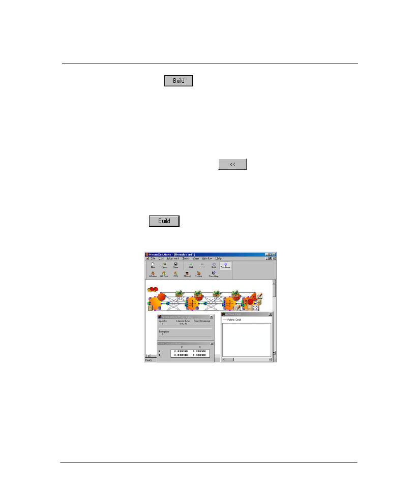
55
8.11 B
UILDING THE
N
ETWORK WITH THE
N
EURAL
B
UILDER
Upon clicking the Build button
from the
Probe Configuration
panel, the
NeuralBuilder opens NeuroSolutions and sends the commands necessary to build the
network, exactly as you have designed it.
Keeping the NeuralBuilder in the Background for Future Use
After the network has been built, the NeuralBuilder minimizes itself to the background.
We recommend that you keep the NeuralBuilder in the background with all of your most
recent settings. Should you decide to change your design, simply return to the
NeuralBuilder, backtrack using the Back button
, make only the necessary
changes, and then re-build the network.
Example
Finally, we are ready to build the Multilayer Perceptron.
9 Click the Build button
.
Within NeuroSolutions itself, you should see the following network being built:
Example MLP Breadboard
Once a breadboard has been built, your first step should be to save it:
9 Go to the File menu and select "Save as…".
Save the breadboard using a name and location of your choice.

56
Chapter 9: N
EURAL
N
ETWORK
T
HEORY
9.1 S
UMMARY OF
N
EURAL
N
ETWORK
T
HEORY
It is not necessary to know the details of neural networks in order to use them, but this
basic introduction can be helpful. A complete coverage of neural network theory can be
found within the interactive book "Neural and Adaptive Systems: Fundamentals Through
Simulations” (ISBN: 0471351679) by Principe, Euliano, and Lefebvre. More information
on this book is available from the NeuroDimension web site at:
http://www.nd.com/products/nsbook.htm
Neural Network Definition
A neural network is an adaptable system that can learn relationships through repeated
presentation of data and is capable of generalizing to new, previously unseen data. Some
networks are supervised, in that a human determines what the network should learn from
the data. In this case, you give the network a set of inputs and corresponding desired
outputs, and the network tries to learn the input-output relationship by adapting its free
parameters. Other networks are unsupervised, in that the way they organize information is
hard-coded into their architecture.
Neural Network Use
Neural networks are used for both regression and classification. In regression, the outputs
represent some desired, continuously valued transformation of the input patterns. In
classification, the objective is to assign the input patterns to one of several categories or
classes, usually represented by outputs restricted to lie in the range from 0 to 1, so that
they represent the probability of class membership.
Important Neural Network Theories
For regression, it can be shown that a single hidden layer Multilayer Perceptron can learn any desired
continuous input-output mapping if there are sufficient numbers of axons in the hidden layer(s).
For classification, Multilayer Perceptrons can learn the Bayesian posterior probability of correct
classification. This means that the neural network takes into account the relative frequency of
occurrence of the classes, giving more weight to frequently occurring classes.
For temporal problems, it can be shown that recurrent networks can follow any desired trajectory over
time.

57
9.2 T
HE
N
EURAL
N
ETWORK
D
ESIGN AND
U
SE
L
IFE
C
YCLE
The Neural Network design and use life cycle is a complex dynamic process with many
steps. However, careful consideration of the following steps can yield a vast improvement
in neural network performance.
1. Understand the Data
Neural networks cannot be used as black boxes, even in the best of circumstances. There
is no substitute for a firm understanding of the data. Explore the data in as many ways as
possible:
a) Try to understand the physical process that produced the data.
b) Plot the data: Plot the individual channels, as well as one channel against another.
c) Examine the statistics: Calculate the within channel mean and variance, as well as
the between channel correlations.
d) Use digital signal processing (DSP) analysis techniques, such as the Fast Fourier
Transform (FFT), to understand the data in the frequency domain.
2. Preprocess the Data
The goal here is to take the insight gained in (1) above, and to encode it into the data.
Examples include:
a) Transform the data so that it better represents "features" of the known physical
process.
b) Transform the data to a more compact representation using universal techniques
such as Principal Component Analysis (PCA) or Kohonen Self-Organizing
Feature Maps (SOFM). Note that these techniques can also be implemented
online at the first layer of a neural network.
c) Eliminate superfluous input channels. It is also possible to identify superfluous
input channels after a network has been trained (see (7) below).
3. Choose a Desired Input-Output Mapping
Decide what the neural network is to accomplish. In particular, what is to be the desired
input-output relationship? Sometimes this can require hand coding of the desired data.
4. Choose a Neural Architecture
(see Choosing a Neural Architecture)
For regression, always start out with a linear network. For classification, always start out
with a linear discriminant classifier. Even if these networks do not perform well, they
provide a baseline comparison for other networks as you graduate in complexity. Also, a

58
consideration here is whether an unsupervised network can perform the desired input-
output mapping.
5. Train the Network
(see Neural Network Training Hints )
If possible, monitor the training with a subset of the training exemplars set aside as a cross
validation set. If the data set is too small to use cross validation, then stop the training
when the learning curve first starts to level off.
6. Repeat the Training
There is a high degree of variability in the performance of a network trained multiple
times, but starting from different initial conditions.
Therefore, the training should be repeated several times, varying the size of the network,
and/or the learning parameters. Among those networks that perform the best (on the
cross validation set, if available), choose the one with the smallest number of free weights.
7. Perform Sensitivity Analysis
Sensitivity analysis measures the effect of small changes in the input channels on the
output, and is computed over the whole training set. It can be used to identify superfluous
input channels. Eliminate those channels and repeat the training process.
8. Test the Network on New Data
This is where you put the network to use. If you have carefully followed the previous
steps, the network should generalize well to new data.
9. Update the Training
Occasionally, when enough new data is accumulated, include old test data in with the
existing training set, and repeat the entire training process.
9.3 C
HOOSING A
N
EURAL
A
RCHITECTURE
Neural networks can be very powerful learning systems. However, it is very important to
match the neural architecture to the problem. As seen previously, the NeuralBuilder
constructs the most popular neural architectures. The chart below is a guide to choosing
one of the NeuralBuilder’s models for your problem.

59
Model
Description
Primary Use or Advantage
Multilayer Perceptron
(MLP)
The most widely used neural
network
General Classification or Regression.
Generalized Feedforward
MLP
MLP plus additional layer-to-
layer forward connections
Additional computing power over
standard MLP.
Modular Feedforward
Several parallel MLP’s that
combine at the output
Reduced number of weights between
layers compared to standard MLP.
Radial Basis Function
(RBF)
Linear combination of
Gaussian Axons
Fast training, simple interpretation of
Gaussian centers and widths.
Jordan and Elman
MLP with non-adaptable
recurrent feedback
Adds fixed memory to the MLP for
simple temporal problems with fixed
temporal dependencies.
Principal Component
Analysis (PCA) Hybrids
Unsupervised PCA at input
followed by a supervised MLP
Project high dimensional redundant
input data onto smaller dimension.
Resulting outputs are orthogonal.
Self-Organizing Feature
Map (SOFM) Hybrid
Unsupervised SOFM at input
followed by a supervised MLP
Project high dimensional data onto
smaller dimension while preserving
neighborhoods.
Time Lagged Recurrent
Locally recurrent layer(s) with a
single adaptable weight
For temporal problems with short
temporal dependencies. Guaranteed
stability, simple interpretation of
recurrent weight in terms of memory
depth of data.
General Recurrent
Fully and partially recurrent
networks
For more difficult temporal problems,
the most powerful neural network, but
also the most difficult to train. Often
become unstable.
CANFIS
Adaptable Fuzzy membership
function at the input
For poorly defined problems. The fuzzy
preprocessing makes the neural
network’s job easier by characterizing
inputs that are not easily discretized,
often resulting in a better overall model.
Support Vector Machine
Trained using the kernel
adatron algorithm.
Strictly used for small to medium sized
classification problems. The SVM is
especially effective in separating sets of
data that share complex boundaries.
Within NeuroSolutions itself, you can manually construct an even wider variety of neural
architectures.

60
9.4 N
EURAL
N
ETWORK
T
RAINING
H
INTS
Here are some key tips for getting better results. Keep in mind that the NeuralBuilder
automatically implements many of these suggestions for you.
Speeding Up Training
For large data sets, use the online weight update.
Updating the network weights after the presentation of each exemplar acts as a random
source of perturbation to the gradient descent, which can help keep the network from
getting stuck in a local minima.
On the hidden layers, use the Tanh non-linearity, not the Sigmoid.
Sigmoids produce zeros, and learning does not occur when the input to a learning element
is zero.
Scale your data by input channel to match the range of the first hidden layer’s transfer function.
Scaling your data by channel to match the first hidden layer’s range can speed up training
because a solution is not far from the initial weight values in the weight space (the relative
magnitudes of the weights before and after training are comparable). For the Tanh non-
linearity, scale the data to lie between –1 and 1.
Use a small learning rate for layers near the output, and an increasingly larger learning rate as you
move back in the network towards the input.
The gradient gets attenuated by each layer as it is backpropagated from the output to the
input, and this can cause layers near the input to learn very slowly.
Try using the Levenberg-Marquardt learning alrgorithm.
This pseudo second-order learning algorithm tends to train in fewer epochs and arrive a
lower error. I may not be practical for very large networks (i.e., several hundred weights or
more).
Improving Generalization
Don’t train forever.
Overtraining can actually degrade performance on the test set. If you can, set aside part of
your training data for cross validation, and stop the training when the performance on the
cross validation set deteriorates. If your data set is too small to afford cross validation,
then stop the training when the learning curve (error vs. epoch) just begins to flatten out.
Repeat the training several times.
Neural networks are highly non-linear and can have many local minima in the weight
space. Repeating the training increases your chance of finding, or getting closer to, the
global minimum.

61
For multi-way classification, where the desired response is either 0 or 1, use a SoftMax at the output
layer (to constrain the outputs to sum to one). Monitor the confusion matrix, in addition to mean
square error, to monitor the training progress.
If you use a SoftMax output, then you can interpret the outputs directly as probabilities,
even for the test set.
For regression, where the desired response varies continuously over some range, use a linear output.
Even if your data is scaled, the larger dynamic range of a linear output will both speed up
learning and improve generalization.
Find the minimum number of total PE’s in the network such that it is still able to learn the problem.
You can either start with a small number of PE’s per layer and then increase until the
network is first able to learn the problem, or you can start with a large number of PE’s
and then decrease until the network no longer learns. The network with the smallest
number of free weights is also the one most likely to generalize well on new data. As a
general rule, start with a network that has approximately one free weight for every ten
exemplars in the training set.
For high-dimensional input data, use a Principal Component Analysis (PCA) layer at the input to
project the input onto a smaller dimension.
The smaller dimensional input reduces the number of free weights in the layers that
follow, which can improve generalization, and the orthogonalization of the input can
speed up training.

62
Chapter 10: A
PPENDIX
10.1 F
ILE
F
ORMAT
R
EQUIREMENTS
Whereas NeuroSolutions can input data in many formats, including binary and bitmaps,
the NeuralExpert and NeuralBuilder require that your data be formatted as follows:
ASCII file format.
Data arranged as columns, which may include inputs, desired outputs, or data that is not used by the
neural network.
Each row contains one exemplar (pattern) of data (with the exception of the first row, which may
contain column headings).
The data elements within each row are separated by tabs, spaces, or commas.
Example
SpecimenNumber,Species,FrontalLip,RearWidth,Length,Width,Depth,Male,Female
142,0,20.6,14.4,42.8,46.5,19.6,1,0
19,1,13.3,11.1,27.8,32.3,11.3,1,0
169,0,16.7,14.3,32.3,37,14.7,0,1
56,1,9.8,8.9,20.4,23.9,8.8,0,1
164,0,15.6,14.1,31,34.5,13.8,0,1
53,1,9.1,8.1,18.5,21.6,7.7,0,1

63
I
NDEX
A
A
DDRESS
.........................................................................................................................................................
V
A
RCHITECTURE
...........................................................................................................................................69
ASCII............................................................................................................................................................73
B
B
READBOARD
I
CONS
..................................................................................................................................31
B
UILDING
.....................................................................................................................................................65
C
C
LASSIFICATION
..........................................................................................................................................18
C
LUSTERING
................................................................................................................................................18
C
OLUMN
........................................................................................................................ 21,
22,
23,
24,
26,
27
C
OMPLEXITY
................................................................................................................................................29
C
OMPONENT
..................................................................................................................................................9
C
ONTACT
........................................................................................................................................................
V
C
ONTENTS
.....................................................................................................................................................7
C
ROSS
V
ALIDATION
........................................................................................................................27,
28,
55
C
YCLE
...........................................................................................................................................................68
D
D
ATA
..........................................................................................20,
21,
22,
23,
24,
25,
26,
27,
52,
53,
55,
73
D
EMOS
....................................................................................................................................................11,
12
D
ENORMALIZATION
.............................................................................................................................41,
42
D
ENORMALIZE
............................................................................................................................................41
D
ESIGN
.........................................................................................................................................................68
D
ESIRED
.................................................................................................................. 23,
24,
25,
26,
27,
53,
63
E
E
.............................................................................................................................................................
V
F
F
ILE
.............................................................................................................. 20,
21,
23,
24,
47,
52,
53,
55,
73
F
INISH
...........................................................................................................................................................65
F
ORMAT
........................................................................................................................................................73
F
OUR
W
AYS TO
C
ONSTRUCT A
N
EURAL
N
ETWORK
..............................................................................16
F
UNCTION
....................................................................................................................................................18
G
G
ENERALIZATION
................................................................................................................................27,
28
S
PEED
......................................................................................................................................................71,
72

64
H
H
ELP
.............................................................................................................................. 13,
14,
15,
18,
46,
51
H
IDDEN
..................................................................................................................................................57,
58
H
INTS
............................................................................................................................................................71
I
I
NPUT
................................................................................................................................... 20,
21,
23,
52,
53
I
NSPECTOR
.............................................................................................................................................33,
34
I
NSTALLATION
...............................................................................................................................................8
I
NSTRUCTIONS
...............................................................................................................................................8
L
L
AUNCH
..................................................................................................................................................17,
50
L
AUNCHING
.................................................................................................................................................11
L
AYER
...............................................................................................................................................57,
59,
60
L
EARNING
..............................................................................................................................................61,
62
L
EARNING
R
ATE
...................................................................................................................................57,
59
L
EARNING
R
ULE
.............................................................................................................................57,
58,
59
L
EVEL
.............................................................................................................................................................2
L
IFE
...............................................................................................................................................................68
L
IST
.................................................................................................................................................................7
L
OCAL
.....................................................................................................................................................39,
40
M
M
INIMA
...................................................................................................................................................39,
40
M
ODEL
.............................................................................................................................................29,
56,
70
M
ODELS
T
OPOLOGY
...................................................................................................................................................51
N
N
ETWORK
........................................................................................................................... 29,
30,
42,
44,
65
N
EURAL
N
ETWORK
........................................................................................................................67,
68,
69
N
EURAL
B
UILDER
...............................................................50,
51,
52,
53,
55,
56,
59,
60,
61,
62,
63,
65,
73
PE..................................................................................................................................................................59
N
EURAL
E
XPERT
.............................................................................17,
18,
20,
21,
23,
24,
26,
27,
28,
29,
73
N
EURO
D
IMENSION
......................................................................................................................................
V
N
EURO
S
OLUTIONS
.......................................................................................................................................1
O
O
NLINE
..................................................................................................................................................13,
15
O
PTIMIZATION
............................................................................................................................................43
O
PTIMIZE
.....................................................................................................................................................42
O
UTPUT
....................................................................................................... 23,
24,
25,
26,
27,
48,
59,
60,
63
P
P
ACKING
........................................................................................................................................................7
P
HONE
............................................................................................................................................................
V

65
P
ROBE
...............................................................................................................................................42,
62,
63
P
ROBES
.........................................................................................................................................................48
P
ROBLEM
..........................................................................................................................................18,
19,
20
P
ROCESSING
E
LEMENTS
............................................................................................................................57
P
RODUCTION
...............................................................................................................................................47
R
R
ECOVERY
....................................................................................................................................................39
R
EGRESSION
................................................................................................................................................18
R
EQUIREMENTS
.............................................................................................................................................7
R
UNNING A
S
IMULATION
...........................................................................................................................37
S
S
ELECTION
...................................................................................................................................................47
S
TART
............................................................................................................................................................50
S
TARTING
.....................................................................................................................................................11
S
TOP
........................................................................................................................................................61,
62
S
UMMARY
...................................................................................................................................................1,
9
S
UPERVISED
.................................................................................................................................................61
S
UPPORT
.........................................................................................................................................................3
S
YMBOL
.........................................................................................................................................................26
S
YMBOLIC
...............................................................................................................................................26,
27
S
YSTEM
...........................................................................................................................................................7
T
T
AG
.............................................................................................................................................21,
23,
24,
26
T
ECHNICAL
....................................................................................................................................................3
T
EST
........................................................................................................................................................28,
46
T
ESTING
.............................................................................................................................. 28,
46,
47,
48,
55
T
ESTING
W
IZARD
............................................................................................................................46,
47,
48
T
HEORY
........................................................................................................................................................67
T
IPS
...............................................................................................................................................................39
T
OPOLOGY
.......................................................................................................................................29,
56,
69
T
RAINING
.................................................................................................... 39,
40,
41,
52,
53,
61,
62,
71,
72
T
YPE
........................................................................................................................................................18,
20
U
U
NINSTALL
...................................................................................................................................................10
V
V
ERIFICATION
.............................................................................................................................................41
W
W
EIGHTS
................................................................................................................................................61,
62
W
ELCOME
......................................................................................................................................................1
Wyszukiwarka
Podobne podstrony:
GETTING STARTED MANUAL
Getting Started
getting started IAOTAGZXANHHC6G Nieznany
(ebook pdf) Matlab Getting started
Part I Getting Started
1 3 Getting started with Data Studio Lab
Getting Started with PostHASTE
Packt Publishing Getting Started with Backbone Marionette (2014)
Getting Started
ANSYS Getting Started Tutorial Workbench
chinas southwest 3 getting started
1 2 Getting started (2)
mr zr getting started
Matlab Getting Started
01 GETTING STARTED
Part I Getting Started
więcej podobnych podstron