Version 7

Getting Started

Manual

OriginLab Corporation

All rights reserved. No part of the contents of this book may be reproduced or transmitted in any form
or by any means without the written permission of OriginLab Corporation.

OriginLab, Origin, and LabTalk are either registered trademarks or trademarks of OriginLab
Corporation. Other product and company names mentioned herein may be the trademarks of their
respective owners.

OriginLab Corporation
One Roundhouse Plaza
Northampton, MA 01060
USA
(413) 586-2013
(800) 969-7720
Fax (413) 585-0126
www.OriginLab.com

Contents

•

Contents

Chapter 1, Introduction

Welcome to Origin .................................................................................................................... 1
Getting Help Using Origin ........................................................................................................ 1
Additional Products Available from OriginLab ........................................................................ 3

OriginPro..................................................................................................................... 3
The Peak Fitting Module............................................................................................. 4
Additional Add-ons..................................................................................................... 5

Chapter 2, Installing and Registering Origin

System Requirements ................................................................................................................ 7
Installing Origin - Single User License ..................................................................................... 7

Upgrading an Existing Version of Origin ................................................................... 7
Required System DLLs ............................................................................................. 12
Un-installing Origin .................................................................................................. 13
Re-installing Origin................................................................................................... 13

Installing Origin - Network License........................................................................................ 14

Installing the Origin 7 Server .................................................................................... 14
Un-installing the Server ............................................................................................ 15
Installing the Origin 7 Clients ................................................................................... 15
Un-Installing a Client................................................................................................ 17

Starting and Registering Origin............................................................................................... 18

Chapter 3, What's New in Version 7

Introduction ............................................................................................................................. 21
Ease-of-Use ............................................................................................................................. 21

Annotations ............................................................................................................... 21
Plotting...................................................................................................................... 25
Analysis..................................................................................................................... 26
Data Import and Handling......................................................................................... 28

Analysis Power........................................................................................................................ 33

New Graph Types ..................................................................................................... 33
Statistical Analysis .................................................................................................... 37
Programming............................................................................................................. 42

Contents

•

Contents

Chapter 4, Getting Started Using Origin

The Origin Workspace............................................................................................................. 45

Menus and Menu Commands.................................................................................... 46
Toolbars..................................................................................................................... 48
Window Types .......................................................................................................... 54
Project Explorer ........................................................................................................ 64
Results Log................................................................................................................ 67
Code Builder ............................................................................................................. 68
Script Window .......................................................................................................... 69

Origin Project Files.................................................................................................................. 70

Saving a Project......................................................................................................... 71
Automatically Creating a Backup ............................................................................. 72
Opening a New Project ............................................................................................. 72
Opening an Existing Project...................................................................................... 73
Opening More than One Project................................................................................ 74
Appending Projects ................................................................................................... 74

Project Windows ..................................................................................................................... 75

Creating a New Window ........................................................................................... 75
Renaming a Window................................................................................................. 76
Hiding a Window ...................................................................................................... 77
Deleting a Window.................................................................................................... 77
Refreshing a Window................................................................................................ 78
Duplicating a Window .............................................................................................. 78
Saving a Window ...................................................................................................... 78
Opening a Window from a File................................................................................. 79

Window Templates.................................................................................................................. 80

Tutorial 1, Plotting Your Data

Introduction ............................................................................................................................. 85
Importing Your Data ............................................................................................................... 85
Designating Worksheet Columns as Error Bars ...................................................................... 89
Plotting Your Data................................................................................................................... 90

Focusing on a Region of Your Graph........................................................................ 91

Customizing the Graph............................................................................................................ 93

Customizing the Data Plot......................................................................................... 93
Customizing the Axes ............................................................................................... 93
Adding Text to the Graph.......................................................................................... 95

Saving Your Project ................................................................................................................ 97

Contents

•

iii

Tutorial 2, Exploring Your Data

Introduction ............................................................................................................................. 99

Data Reader............................................................................................................... 99
Screen Reader ......................................................................................................... 100
Data Selector ........................................................................................................... 101
Enlarger Tool and Undo Enlarge ............................................................................ 102
Zoom In and Zoom Out........................................................................................... 104
Region of Interest (Image Data).............................................................................. 105
Masking................................................................................................................... 106

Getting Started....................................................................................................................... 108
Transforming Column Values ............................................................................................... 109
Sorting Worksheet Data ........................................................................................................ 110
Plotting a Range of the Worksheet Data................................................................................ 112
Masking Data in the Graph.................................................................................................... 113
Performing a Linear Fit on the FLUOR Data Plot................................................................. 115
Saving the Project.................................................................................................................. 119

Tutorial 3, Creating Multiple Layer Graphs

121

Introduction ........................................................................................................................... 121
Opening the Project File........................................................................................................ 123
Origin's Multiple Layer Graph Templates............................................................................. 123
Designating Multiple X Columns in the Worksheet.............................................................. 127
Creating a Multiple Layer Graph........................................................................................... 128

Arranging Layers in the Graph Window................................................................. 131
Adding Data to the New Layers.............................................................................. 133
Linking Axes........................................................................................................... 134

Customizing the Legend........................................................................................................ 136
Saving the Graph as a Template ............................................................................................ 140

Tutorial 4, Nonlinear Curve Fitting

141

Introduction ........................................................................................................................... 141
Fitting from the Menu ........................................................................................................... 141
Fitting Using the Tools.......................................................................................................... 143
Fitting Comparison................................................................................................................ 144
The Fitting Wizard ................................................................................................................ 145
The Advanced Fitting Tool ................................................................................................... 146

The Basic Mode ...................................................................................................... 146
The Advanced Mode ............................................................................................... 147

Fitting a Data Set Using Your Own Function ....................................................................... 148

Opening the Project File.......................................................................................... 148
Defining a Function................................................................................................. 149
Assigning the Function Variables to the Data Sets ................................................. 150
Simulating Curves to Initialize the Parameter Values............................................. 152
Fitting the Data........................................................................................................ 154
Creating a Worksheet With the Fitting Results and Exiting the Fitter .................... 155

Contents

•

Contents

Tutorial 5, Creating 3D Surface Graphs

159

Introduction to Matrices ........................................................................................................ 159
Converting a Worksheet to a Matrix ..................................................................................... 162

Selecting the Type of Conversion ........................................................................... 163

Creating a 3D Surface Graph................................................................................................. 166
Customizing the Graph.......................................................................................................... 168

Changing the Color Map Values ............................................................................. 168
Changing the Color Map Colors ............................................................................. 170
Adding Contours to the Color Map Surface Graph................................................. 172
Changing the Perspective of the Graph ................................................................... 173

Tutorial 6, Creating Presentations with the Layout Page

175

Introduction ........................................................................................................................... 175
Adding Graphs, Worksheets and Text to the Layout Page .................................................... 176

Opening the Project File.......................................................................................... 176
Creating a New Layout Page................................................................................... 177
Adding Pictures and Text to a Layout Page ............................................................ 178

Customizing the Appearance of the Layout Page.................................................................. 182

Arranging Pictures on the Layout Page................................................................... 182
Editing the Pictures in the Layout Page .................................................................. 184

Exporting the Layout Page .................................................................................................... 187

Tutorial 7, Working with Excel in Origin

191

Introduction ........................................................................................................................... 191
Opening an Excel Workbook in Origin ................................................................................. 191
Plotting an Excel Workbook in Origin .................................................................................. 193

Creating a Graph Using the Select Data for Plotting Dialog Box ........................... 194
Creating a Data Plot by Dragging Data Into a Graph.............................................. 196
Creating a Graph Using Origin’s Default Plot Assignments................................... 197

Saving an Excel Workbook in Origin.................................................................................... 198

Tutorial 8, Programming in Origin

201

Introduction ........................................................................................................................... 201
Creating a New Source File................................................................................................... 202
Coding Your Function ........................................................................................................... 204
Compiling and Testing the Function ..................................................................................... 205
Using the Function in Origin ................................................................................................. 207

Index

211

Chapter 1, Introduction

Welcome to Origin

•

Chapter 1, Introduction

Welcome to Origin

Thank you for purchasing Origin version 7! This manual is provided to
familiarize you with the fundamentals of Origin in a minimal amount of
time. The manual provides information for new and upgrade users,
including:
=> A summary of the major new features in version 7.
=> An overview of the major Origin concepts and terminology.
=> Tutorials covering a broad range of Origin topics.
This manual also provides installation and registration assistance. For
additional help using Origin, review the Origin Help file (Help:Origin)
or visit the OriginLab web site at www.OriginLab.com.

Getting Help Using Origin

If you have a question about using Origin, assistance is available from
several different sources.

From the Software
=> The status bar in the Origin window provides text clarifying the
function of toolbar buttons, tool elements, and menu commands. It also
displays Origin status messages.

Figure 1: The Status Bar Messages

Chapter 1, Introduction

•

Getting Help Using Origin

=> The Origin Help contains information on all of Origin’s features. To
open the Origin Help, select Help:Origin or press F1. If a dialog box is
open when you press F1, the Help opens displaying information specific
to the dialog box.
Programming Help is also available from the Help:Programming
submenu. Select Program Guide to learn general tips and strategies on
programming in Origin. Select Origin C Reference to find information
on a specific Origin C class or function. Select LabTalk Reference to
find information on the LabTalk programming language.

Viewing Origin's Help
files requires Internet
Explorer version 4.0 or
higher.

Important Note about Origin's Help Files: The Origin Help files are
compiled HTML Help. To view these Help files, you must have
Internet Explorer version 4.0 or higher installed on your computer. (We
recommend having Internet Explorer version 5.0 or higher installed.)
Internet Explorer need not be your default browser, but it must be
installed.

=> Sample Origin projects and data files are provided with Origin.
These files are located in the Origin \Samples subfolder. Sample projects
show you how to perform analysis routines, create custom graphs, and
program routines in Origin.

From the Manuals
=> This Getting Started Manual includes a "Getting Started Using
Origin" section with basic information on using Origin. Tutorials are
also provided which step you through common Origin operations.
=> The Programming Guide provides general tips and strategies on
programming in Origin.

From the Web Site
You can access helpful areas of the OriginLab web site by selecting
Help:Origin on the Web. This menu command opens a submenu
providing fast access to a number of useful areas. These resource pages
include support, custom tools, the graph gallery, a user forum, and the
OriginLab home page. To access the OriginLab home page directly from
your browser, go to www.OriginLab.com.

From Your Origin Technical Support Representative
OriginLab and our team of international support representatives are
committed to providing high quality technical support to our registered
users of Origin. To contact OriginLab Technical Support or to find out
how to contact your local support representative, select Help:Origin on
the Web:Technical Support. Alternatively, go to www.OriginLab.com
and click the Technical Support link.

Chapter 1, Introduction

Additional Products Available from OriginLab

•

=> Customers with local technical support representatives can find
contact information on the OriginLab technical support web pages.
=> If OriginLab is your technical support representative, you can submit
a technical question to OriginLab from the web site.
Additionally, if OriginLab is your technical support representative, you
can contact OriginLab Technical Support at tech@originlab.com.
Phone: 1-800-969-7720 or 1-413-586-2013

Additional Products Available from OriginLab

OriginLab provides two major products, Origin and OriginPro. In
addition, OriginLab provides custom tools and modules that enhance
Origin and OriginPro.

OriginPro

OriginPro includes all the features found in Origin. Additionally,
OriginPro is an application development environment for building
custom analysis applications based on Origin. After development,
custom applications can be run on the standard Origin version or the
OriginPro version.

Create Sophisticated Custom Interfaces
=> Create dialog boxes, tabbed tools, and wizards using OriginPro’s
Dialog Builder.
=> Select controls from industry standard development tools.
=> Save wizard procedures as a toolbar button.
=> Add your own menus and menu commands to the Origin menu bar.

Powerful Programming Environment with Origin C (Origin C is also
part of standard Origin)
=> ANSI C with some C++ features.
=> String, vector, matrix, complex, complex matrix support built-in.
=> Access to Origin objects such as worksheets, data plots, and Project
Explorer.
=> Essential elements of the Numerical Algorithms Group (NAG

)

numerical library included for advanced computation.
=> Code Builder environment provides syntax coloring, debugging with
breakpoints, and output windows.

Chapter 1, Introduction

•

Additional Products Available from OriginLab

=> Add custom classes into Origin C classes with external DLL. (This
feature is only available in OriginPro.)

Design Dynamic Data Exchange (DDE) Applications
=> Program your Visual Basic or Visual C++ applications to send data
to Origin to display complex graphs in real time.
=> Use Origin as a graphics server.

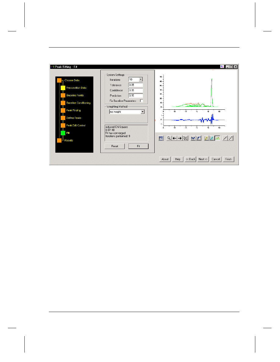
The Peak Fitting Module

Work in chromatography, spectroscopy, engineering, pharmacology, and
other fields frequently requires analysis of data sets exhibiting multiple
peaks. Analysis of multi-peak data is particularly difficult when peaks
overlap, or when data are "noisy." The Peak Fitting Module (PFM)
provides the tools needed for serious peak analysis, including:
=> Data filtering.
=> Automatic and/or manual baseline and peak detection.
=> Built-in or user-defined curve-fitting functions.
=> Highly accurate nonlinear least squares curve fitting.
=> Publication-quality output.
The PFM provides a wizard interface to simplify peak analysis. You can
run the PFM on Origin or OriginPro.

Chapter 1, Introduction

Additional Products Available from OriginLab

•

Figure 2: The Peak Fitting Module

Additional Add-ons

In addition to the Peak Fitting Module, OriginLab offers custom tools
and modules that are available from the OriginLab web site
(www.OriginLab.com). Some tools are available free of charge and
others are available at a cost. The tools add specific enhancements to
Origin and OriginPro.
Most of the tools and modules are provided in a special file format with a
.OPK extension. After downloading the file, these tools and modules are
easily installed by dragging the file from Windows Explorer onto your
running copy of Origin or OriginPro.

Chapter 1, Introduction

•

Additional Products Available from OriginLab

Chapter 2, Installing and Registering Origin

System Requirements

•

Chapter 2, Installing and

Registering Origin

System Requirements

Origin version 7 requires the following minimum system configuration:
Microsoft Windows 95 or later or Windows NT 4.0 or later.
133 MHz or higher Pentium compatible CPU.
64 MB of RAM.
CD-ROM drive.
50 MB of free hard disk space.
Internet Explorer version 4.0 or later (we recommend version 5.0 or
later). Internet Explorer need not be your default browser, but it must be
installed for viewing Origin's compiled HTML Help.

Installing Origin - Single User License

For network installation
information, see
"Installing Origin -
Network License" on page
14.

To install a new copy of Origin or OriginPro, or to upgrade an existing
copy, insert the Origin 7 CD into your CD-ROM. A window opens with
a number of options, including installing Origin. Click the link to install
Origin. If the CD does not start automatically, browse the CD and run
ORIGINCD.EXE directly.
The setup program prompts you to type in your Origin serial number
and license key. These numbers are located inside your registration card
in the Origin product package.

Upgrading an Existing Version of Origin

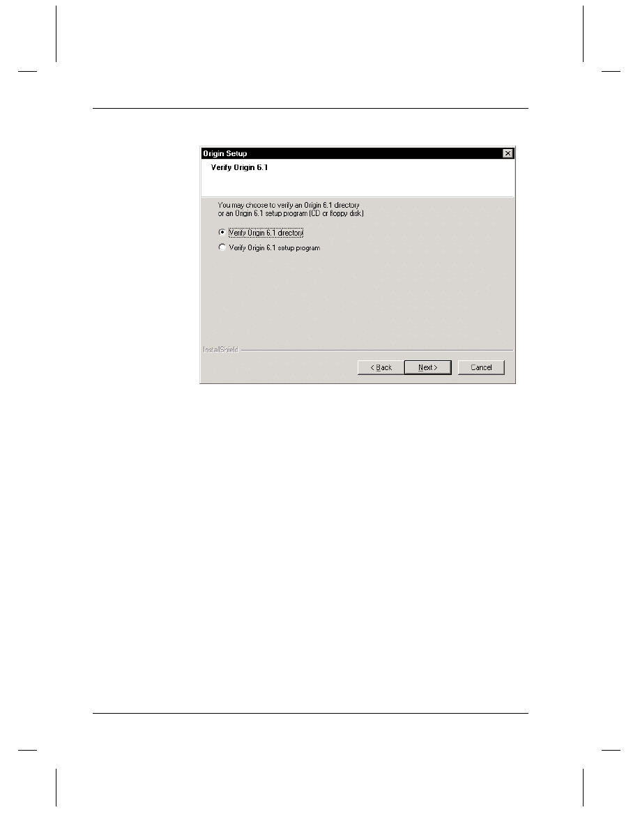
After entering your serial number and license key, the Upgrade setup
program will verify that the previous version of Origin is installed on
your computer. If the Upgrade setup program does not automatically
find this version, it opens the following dialog box.

Chapter 2, Installing and Registering Origin

•

Installing Origin - Single User License

Figure 1: Verifying a Previous Version

This dialog box allows you to instruct the Upgrade setup program to
perform the version verification from a folder on your hard disk or from
the previous version's CD or floppy disk (if the previous version is not
installed on your computer).
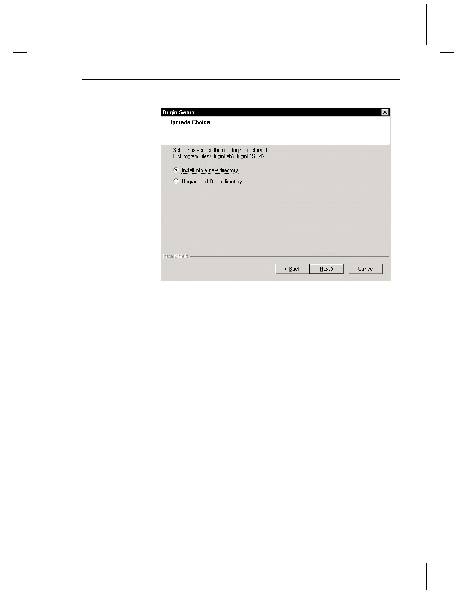
After verification of the previous version, the Upgrade setup program
offers you the option to either upgrade your existing copy of Origin, or to
install Origin 7 into a new folder, leaving the existing copy of Origin
unaltered. To learn more about these options, see Table 1 on page 11.

Chapter 2, Installing and Registering Origin

Installing Origin - Single User License

•

Figure 2: Upgrading an Existing Folder or Installing into a New Folder

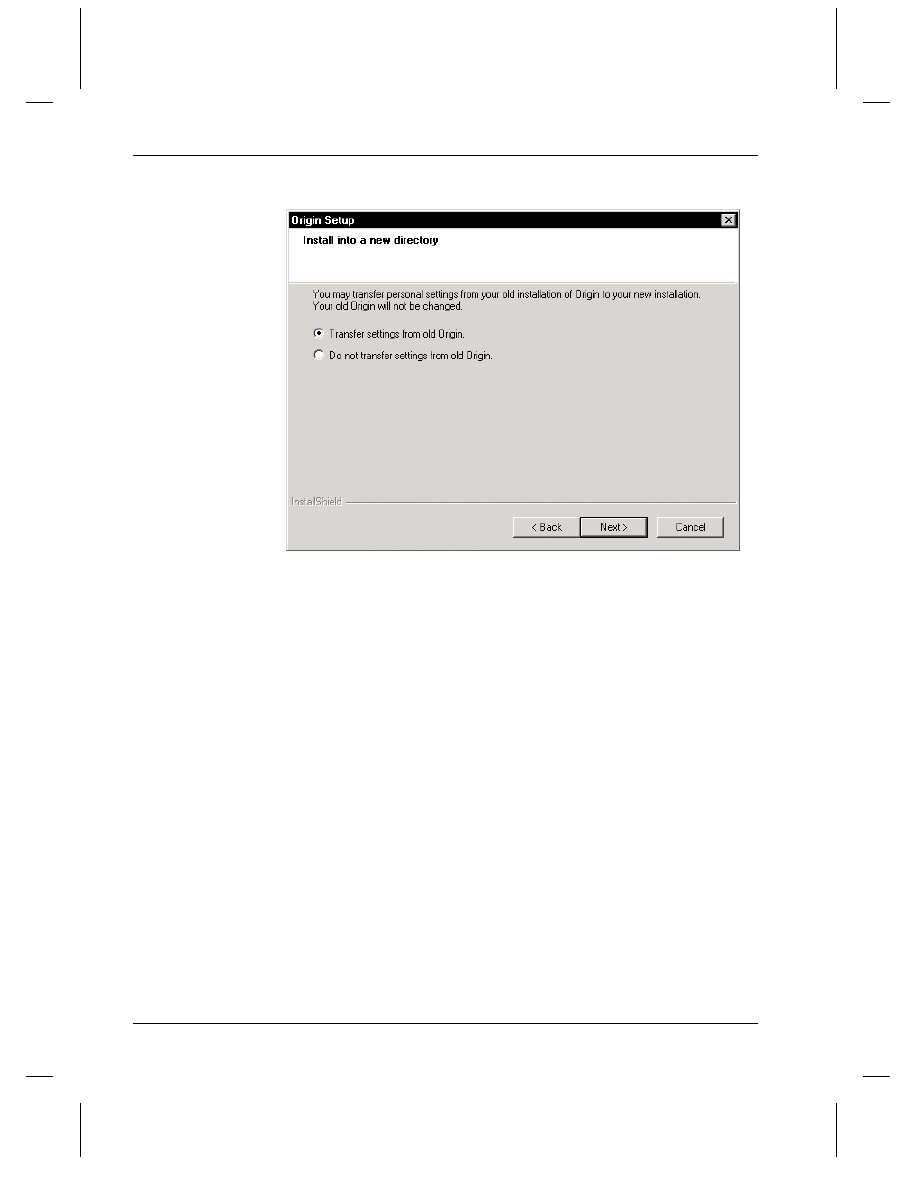
If you install Origin 7 into a new folder, you have the option to:
=> Copy your user-defined fitting functions to the new program folder's
\FitFunc subfolder.
=> Copy any modified built-in files to the new program folder's
\Modified Files subfolder. (Built-in files are files that were installed by
your previous Origin installation. For a list of the built-in file types that
can be modified, see the following table.)
=> Copy any user-defined toolbar settings to the new program folder.
To learn more about this option, see Table 1 on page 11.

Chapter 2, Installing and Registering Origin

•

Installing Origin - Single User License

Figure 3: Installation Option to Transfer Previous Settings

Chapter 2, Installing and Registering Origin

Installing Origin - Single User License

•

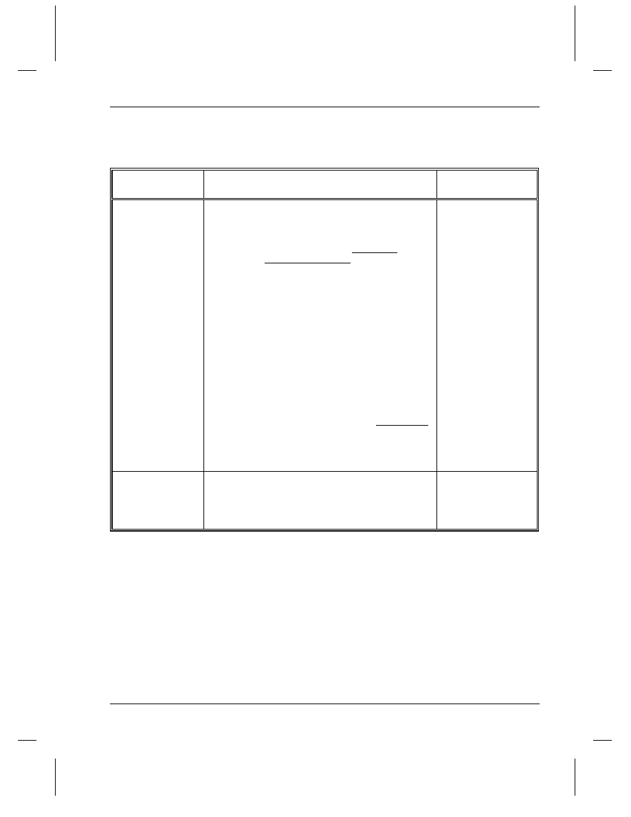
The following table summarizes your upgrade installation options.

Table 1: Upgrade Installation Options

Upgrade Option

Description

When to Choose

this Option

Install into a new
folder, transfer
previous Origin
settings.

1) You are given the option to modify the default program
folder name.
2) Origin is installed into this new folder.
3) The install program then copies all built-in files of the
following type that you have modified in your previous
version of Origin to a \Modified Files subfolder in your new
Origin 7 program folder. This includes template (OTW,
OTP, OTM), script (OGS), initialization (INI),
configuration (CNF), Origin project (OPJ), data (DAT,
etc.), and fitting function (FDF) files. Your modified file in
the original location is left unaltered.
4) User-defined toolbar settings are copied from your
previous version of Origin to your new Origin 7 program
folder. The user-defined toolbar settings in the original
location are left unaltered.
5) User-defined fitting functions are copied into the
\FitFunc folder in your new Origin 7 program folder.
6) Other user-created files (excluding user-defined fitting
functions) that are not modified built-in files are not copied
from your previous version of Origin. For example,
templates, Origin projects, data files, and script files that are
not provided as part of the previous version are not copied
over.

This is the
recommended upgrade
installation option.
This option leaves your
previous Origin
installation unaltered,
but transfers your
custom settings to the
new installation.
If you select this option,
do not delete your
previous Origin
installation until you
have copied any needed
user-created files to the
new program folder.

Install into a new
folder, do not transfer
previous Origin
settings.

1) You are given the option to modify the default program
folder name.
2) Origin is installed into this new folder.
3) Your previous version of Origin is left unaltered.

Select this option if you
do not want any of your
custom settings
transferred to the new
installation.

Chapter 2, Installing and Registering Origin

•

Installing Origin - Single User License

Upgrade Option

Description

When to Choose

this Option

Upgrade previous
Origin folder.

1) You are not given the option to change the program
folder name. Thus, if the previous path was C:\Program
Files\OriginLab\Origin61, it remains the same after your
upgrade. If you change the path after installation, then the
Add/Remove program (see "Un-installing Origin" on page
13) will be unable to find your Origin files. (Note: If you
want to rename your program folder name, do this before
installing the upgrade.)
2) All built-in files of the following type that you have
modified are copied into a \Modified Files subfolder. This
includes template (OTW, OTP, OTM), script (OGS),
initialization (INI), configuration (CNF), Origin project
(OPJ), data (DAT, etc.), and fitting function (FDF) files.
During the upgrade installation, your modified file in the
original location is replaced with the Origin 7 version of the
file.
3) User-created files that are not modified built-in files
(such as new templates and new fitting functions) are not
altered or moved during the upgrade.
4) User-defined toolbars remain available after upgrading.

Select this option if you
are low on disk space.

Required System DLLs

Origin requires the following three system DLLs to run properly:
Mfc42.dll

File Version: 6.00.8665.0 or later

Msvcrt.dll

File Version: 6.00.8797.0 or later

Comctl32.dll File Version: 5.8 or later
These DLLs are most commonly installed to the \Windows\System
folder (Windows 95/98/ME/XP) or the \Windows\System32 folder
(Windows NT/2000). To check the version of any DLL, locate the file
using the Windows Explorer or the Find program, right-click on the DLL
file, select Properties from the shortcut menu, and then select the
Version tab in the Properties window.
During the Origin installation, the setup program will update the DLLs if
older versions are present. If an older version is in use and can not be
replaced during installation, then a reboot is required after installation.
The setup program will inform you of this. Furthermore, if an older
version of a DLL is found, you are given the option to save a copy of the
older version in your Origin \OldSystemDLLs subfolder.
There may be cases where the setup program fails to update the system
DLLs. If this occurs, you can download the DLLs from the Technical
Support area of the OriginLab web site (www.OriginLab.com).

Chapter 2, Installing and Registering Origin

Installing Origin - Single User License

•

Un-installing Origin

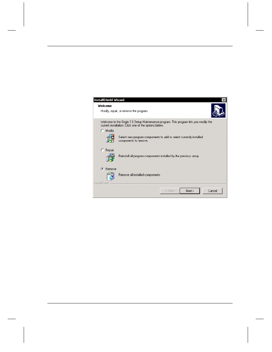
To remove Origin from your computer, run the Origin 7 Add/Remove
program. This program opens the following dialog box. Select the
Remove option.

Figure 4: Un-installing Origin

The Remove option copies all built-in files of the following type that you
have modified into a \Modified Files subfolder. This includes template
(OTW, OTP, OTM), script (OGS), initialization (INI), configuration
(CNF), Origin project (OPJ), data (DAT, etc.), and fitting function (FDF)
files. It then removes all installed files (excluding the \Modified Files
subfolder). User-created files that are not modified built-in files (such as
new templates and new fitting functions) are not removed during this
process.

Re-installing Origin

To re-install Origin, first un-install Origin by running the Origin 7
Add/Remove program and selecting the Remove option (see the previous
topic). Then insert the Origin 7 CD into your CD-ROM and click the
link to install Origin.

Chapter 2, Installing and Registering Origin

•

Installing Origin - Network License

Origin 7 supports a server-based network which can have either machine-
based clients, roaming-user clients, or both. The server must be installed
to a server machine running Windows NT 4.0, 2000, XP or a later
version, and the server machine must use the TCP/IP network protocol.
Client machines must have Windows 95, 98, ME, NT 4.0, 2000, XP or a
later version installed.

Installing the Origin 7 Server

You must run the Server setup program on the server computer - you can
not run it on a remote computer. Additionally, you must log on to an
account that has administrator privileges on the local computer. The
server can be installed anywhere on the server machine that is writable.
After installing the Origin server, it can be shared as read-only.
To install a new copy of the Origin 7 server or to upgrade an existing
version of an Origin server, insert the Origin 7 CD into your CD-ROM.
A window opens with a number of options, including installing Origin.
Click the link to install Origin. If the CD does not start automatically,
browse the CD and run ORIGINCD.EXE directly.
The Server setup program prompts you to type in your Origin serial
number and license key. These numbers are located inside your
registration card in the Origin product package.
If you are upgrading a server installation, you will also be asked if you
want to upgrade your existing version or install the Origin 7 server into a
new folder, leaving the existing copy unaltered. For information on these
upgrade options, see "Upgrading an Existing Version of Origin" on page
7.
After completing the installation, the Origin 7 server is a full working
version of Origin 7. However, the Origin 7 server does not need to be
running for Origin 7 clients to be able to run.

Un-installing the Server

To remove an Origin 7 server, run the Origin 7 Server Add/Remove
program. Select the Remove option in the dialog box that opens. This
option copies all built-in files of the following type that have been
modified into a \Modified Files subfolder. This includes template (OTW,
OTP, OTM), script (OGS), initialization (INI), configuration (CNF),
Origin project (OPJ), data (DAT, etc.), and fitting function (FDF) files.
It then removes all installed files (excluding the \Modified Files
subfolder). User-created files that are not modified built-in files (such as

Chapter 2, Installing and Registering Origin

Installing Origin - Network License

•

new templates and new fitting functions) are not removed during this
process.

Installing the Origin 7 Clients

After the server installation is complete, the Origin server folder includes
a \ClientSetup subfolder that contains a client setup program. The client
setup icon can be double-clicked by the client to install the Origin client.
Alternatively, you can mail the client users an active link to the client
setup program.
If installing to a Windows NT or Windows 2000 computer, you should
log on to an account that has administrator privileges on the client
computer. You do not have to run the Client setup program on the client
computer, but if you run it on a remote computer you must manually
verify that the client computer has the correct version of all required
system DLLs (see "Required System DLLs" on page 12).
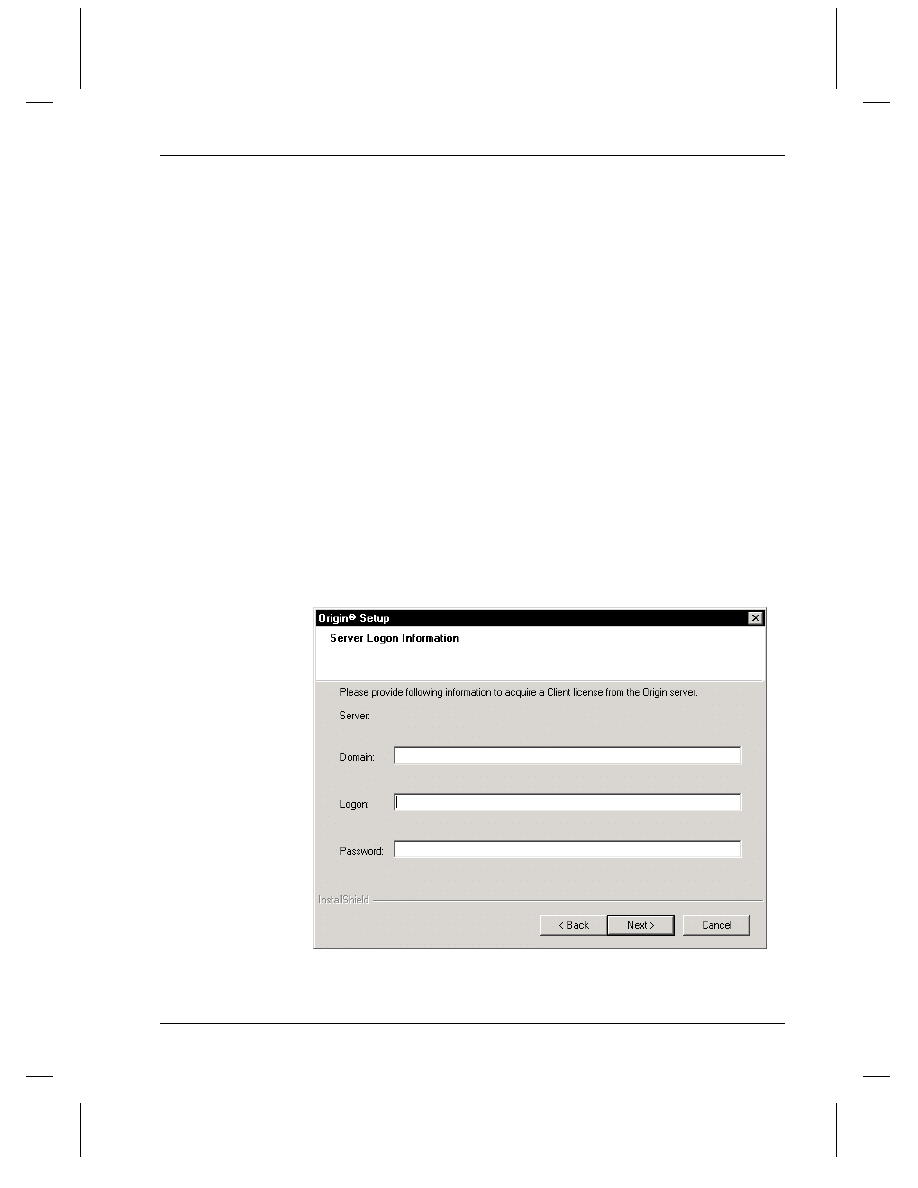
During the client installation, you will be asked to enter the network
license serial number and a client installation folder path. You will also
be asked to enter the server logon information shown in the following
figure.

Figure 5: Server Logon Information

Chapter 2, Installing and Registering Origin

•

Installing Origin - Network License

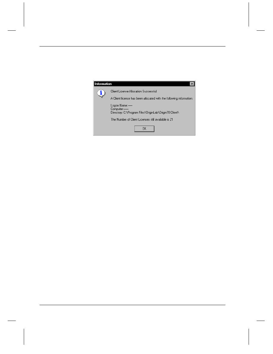
After successful verification, the following dialog box indicates the client
license was successfully allocated.

Figure 6: Successful Allocation of the Client License

If you are upgrading a client installation, you will also be asked if you
want to upgrade your existing version or install the Origin 7 client into a
new folder, leaving the existing copy of Origin unaltered. For
information on these upgrade options, see "Upgrading an Existing
Version of Origin" on page 7.

Installing a Machine-Based or Roaming-User Origin Client
Origin 7 supports a server-based network which can have either machine-
based clients, roaming-user clients, or both. If you log on to any
Windows computer and specify a user account that is not set up as a
roaming-user account (on the Windows NT/2000 Domain Controller)
and install an Origin 7 client, that client installation will be machine-
based. In order to use that particular Origin client you will have to log on
to that machine.
If you log on to any Windows computer and specify a user account that is
set up as a roaming-user account (on the Windows NT/2000 Domain
Controller) and install an Origin 7 client, the client installation of Origin
will be a roaming-user client if the following conditions are met:
=> When asked to enter the path to the Origin 7 client software folder
during the client installation, you must ensure that the path will be valid
no matter which computer is logged on to. You can either enter a UNC
path to the client folder (\\ComputerName\ShareName\...\Origin 7.0
Client) or enter a mapped drive path (H:\Origin 7.0 Client) that is always
valid whenever you log on to that roaming-user account. This condition
is minimally restrictive since UNC paths are absolute and mapped drives,
while relative, are stored as part of a roaming-user's profile.
=> During the client installation you should choose the Personal
(<UserName>) radio button when asked which location you want the

Chapter 2, Installing and Registering Origin

Starting and Registering Origin

•

Origin 7 client program folder to be installed to. This ensures that the
program icons will become part of the roaming-user's profile.
=> You must ensure that the correct version of all required system DLLs
are installed on any computer on which you intend to run an Origin
client. One way to do this is to run the Client setup on each computer
that you will be using a roaming Origin client. This will ensure that the
correct system DLLs are there. You can then uninstall the Origin client
and the updated system DLLs will remain. Alternatively, you can
manually check that the correct DLLs are present. For more information
on manually checking, see "Required System DLLs" on page 12.
Once the pathing, program folder location, and system DLL conditions
are met, Windows will automatically manage the Origin client for that
roaming-user account. You will have complete access to the installed
Origin 7 client no matter which computer you log on to.

Un-Installing a Client

To remove an Origin 7 client from your computer, run the Origin 7
Client Add/Remove program. Select the Remove option in the dialog
box that opens. This option copies all built-in files of the following type
that you have modified into a \Modified Files subfolder. This includes
template (OTW, OTP, OTM), script (OGS), initialization (INI),
configuration (CNF), Origin project (OPJ), data (DAT, etc.), and fitting
function (FDF) files. It then removes all installed files (excluding the
\Modified Files subfolder). User-created files that are not modified built-
in files (such as new templates and new fitting functions) are not
removed during this process.

Starting and Registering Origin

To start Origin, click Start, then select Programs. Point to the Origin 7
folder and select the Origin 7 (or OriginPro 7) program icon from the
submenu.
=> If this is a new installation, if you are upgrading from a version prior
to 6.1, or if you are upgrading from version 6.1 but did not enter a
registration ID in your 6.1 program, then the OriginLab Registration
dialog box displays after you start Origin.
=> If you are upgrading from version 6.1 and you had entered a
registration ID in your Origin 6.1 program, then Origin starts without
displaying the OriginLab Registration dialog box. In this case, your
registration ID is already entered in your upgrade. You can verify this by
selecting Help:About Origin. You registration ID should be listed in
the About Origin dialog box.

Chapter 2, Installing and Registering Origin

•

Starting and Registering Origin

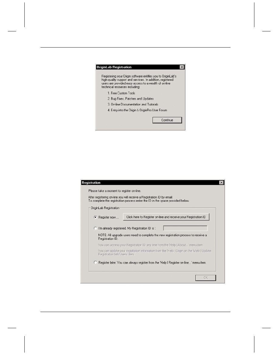
Figure 7: The OriginLab Registration Dialog Box

This dialog box reviews the benefits of registering Origin 7. These
benefits include receiving technical support and having access to services
that are available from the OriginLab web site (www.OriginLab.com).
When you click Continue, the Registration dialog box opens.

Figure 8: The Registration Dialog Box

Chapter 2, Installing and Registering Origin

Starting and Registering Origin

•

=> If you are upgrading from version 6.1 and you had entered a
registration ID in your Origin 6.1 program, then this dialog box does not
display because your upgrade is already registered.

If you do not have web
or email access,
contact your Origin
representative to
complete the
registration process.

=> In all other cases, you must register your copy of Origin by entering
your registration ID (a registration ID is not the same as a serial number
or a license key). If you do not have a registration ID, then click the
associated button in the Registration dialog box. This button starts your
browser and takes you to the OriginLab registration web page. After
you complete the registration form on this web page, you will be sent an
email message notifying you of your registration ID. Type this
registration ID in the Registration ID text box on the Registration dialog
box. Once you enter your registration ID in Origin, both your serial
number and registration ID will display in the About Origin dialog box
(Help:About Origin).

Chapter 2, Installing and Registering Origin

•

Starting and Registering Origin

Chapter 3, What's New in Version 7

Introduction

•

Chapter 3, What's New in

Version 7

Introduction

Origin 7 offers new features that make Origin easier to use and provide
increased analysis power. The following sections introduce the major
new features in version 7. For more information on a feature, review the
Origin Help file (Help:Origin). Additionally, review the Release Notes
provided with the product.

Ease-of-Use

Annotations

Text Editing

Origin 7 provides enhanced annotation tools including in-place text
editing and toolbar button access to common formatting options.
=> To create a new text label, right-click and select Add Text from the

shortcut menu or click the Text Tool button

and then click at the

desired location. Then begin typing the text. As you type your text,
formatting options are available from the Format toolbar and color
control is available from the Style toolbar.

Figure 1: The Format and Style Toolbars

Chapter 3, What's New in Version 7

•

Ease-of-Use

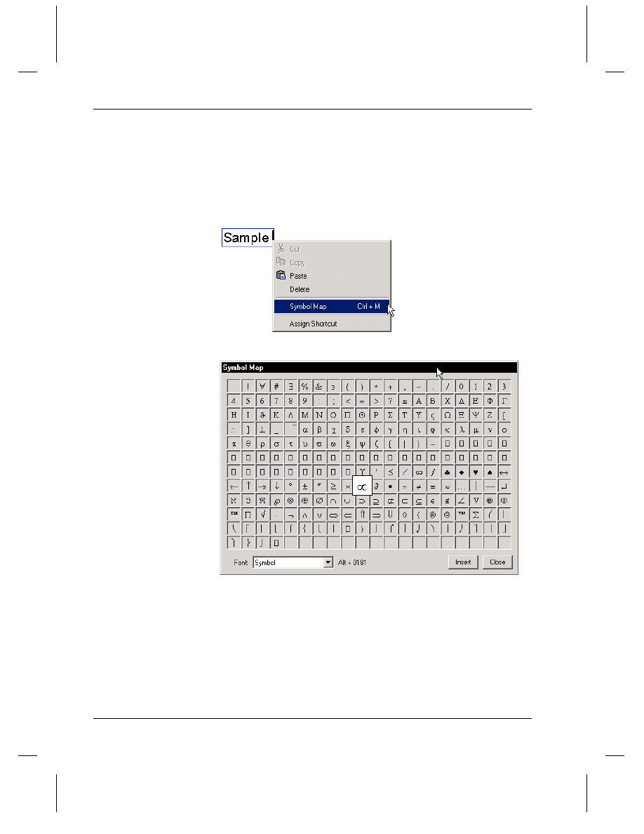
If no text is currently highlighted, the formatting/color option begins at
the current cursor location. Otherwise, the formatting/color applies to the
highlighted text only. You can also add characters from a selected font
set by right-clicking while in in-place editing mode and selecting Symbol
Map from the shortcut menu (or by pressing CTRL+M).

Figure 2: Adding Characters from a Selected Font Set

To exit the text entering and editing mode, click off the label or press
ESC.
=> To edit an existing text label, double-click to enter the in-place
editing mode. (Tip: To temporarily turn off the rotation when you in-
place edit rotated labels, select Tools:Options to open the Options dialog
box. Select the Text Fonts tab and then select the Do Not Rotate Text
While In-Place Editing check box.)

Chapter 3, What's New in Version 7

Ease-of-Use

•

=> To resize a text label, click once on the label and then select the
desired font size from the combo box on the Format toolbar.

Alternatively, click the Increase Font or Decrease Font buttons
on this toolbar. You can also drag a control handle to resize the label.
=> To rotate a text label, click once on the label, pause long enough to
avoid a double-click (about a second), and then click a second time on
the label. A rotation symbol

displays in the middle of the label and

rotation handles display at the corners of the label. Click on a rotation
handle and rotate the label as desired. (You can also specify a specific
rotation angle in the Text Control dialog box.)
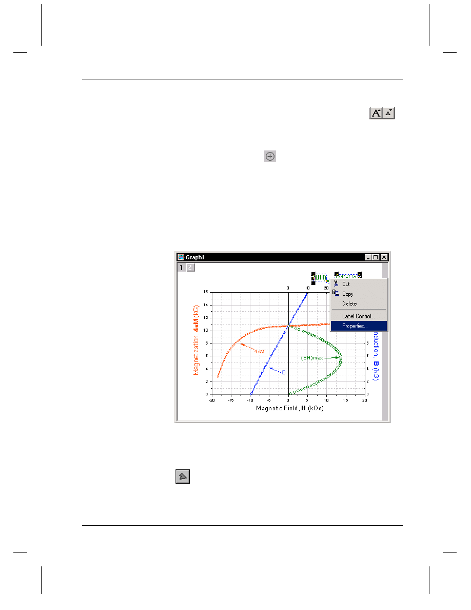
=> To access the Text Control dialog box, right-click on the text label
and select Properties from the shortcut menu. Alternatively, press
CTRL while double-clicking on the label.

Figure 3: Opening the Text Control Dialog Box

Drawing

Four new drawing tools have been added to the Tools toolbar in Origin 7:

Polygon Tool: To draw a polygon, click on the tool and then click

in the window at each of the corner locations for the polygon. Either
double-click at the last location or click once and then press ESC.

Chapter 3, What's New in Version 7

•

Ease-of-Use

Region Tool: To draw a region, click on the tool and then click

and drag the desired region. Release the mouse button to complete the
operation.

Polyline Tool: To draw a polyline, click on the tool and then click

in the window at each of the corner locations for the polyline. Either
double-click at the last location or click once and then press ESC.

Freehand Draw Tool: To draw a freehand line, click on the tool

and then click and drag the desired line. Release the mouse button to
complete the operation.
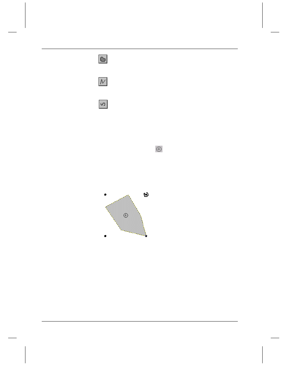
All of Origin's drawing objects can be rotated and skewed. Additionally,
individual points can be moved.
=> To rotate an object, click once on the object, pause long enough to
avoid a double-click (about a second), and then click a second time on
the object. A rotation symbol

displays in the middle of the object

and rotation handles display at the corners of the object. Click on a
rotation handle and rotate the object as desired.

Figure 4: Rotating an Object

Click and rotate.

=> To skew an object, click once on the object, pause long enough to
avoid a double-click (about a second), and then click a second time on
the object. Pause again and then click a third time on the object.
Triangular skew handles display at the corners of the object. Click on a
skew handle and drag as desired.

Chapter 3, What's New in Version 7

Ease-of-Use

•

Figure 5: Skewing an Object

Click and drag a handle.

=> To move points in an object, follow the "skew" procedure and then
click one more time (a total of four clicks with pauses in between).
Handles appear on moveable points. Drag the desired points to new
locations.

Figure 6: Moving an Object's Points

Click and drag a handle.

Additionally, when a drawing object is selected, the Style toolbar buttons
are available for customizing the object's display. For closed objects, this
includes the pattern and fill color controls.
Additional object controls are available from the Object Control dialog
box which is accessed by double-clicking on the object.

Plotting

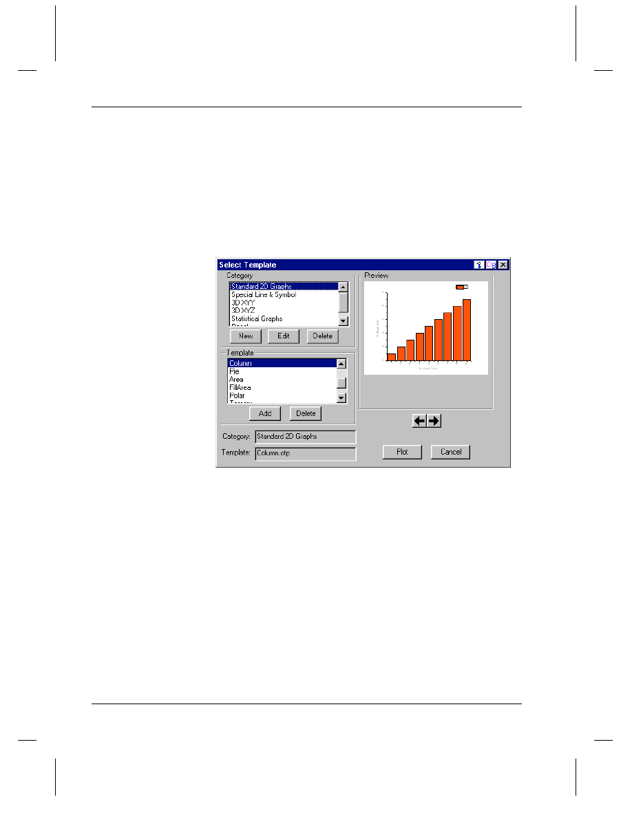
Template Library Tool

Origin provides a Template Library tool for categorizing and accessing
graph templates. To open the Template Library tool when a worksheet or

Chapter 3, What's New in Version 7

•

Ease-of-Use

an Excel workbook is active, select Plot:Template Library. In addition
to organizing graph templates, you can also use the tool to plot your
worksheet or Excel workbook data. If you highlighted data in the
worksheet or workbook before opening the tool, and your data selection
is appropriate for the template you've selected, then click the Plot button
to plot the data into the template. If you did not highlight data or if your
selection was not appropriate for the template you've selected, then click
the Plot button to open an intermediary dialog box for data selection.

Figure 7: The Template Library Tool

Analysis

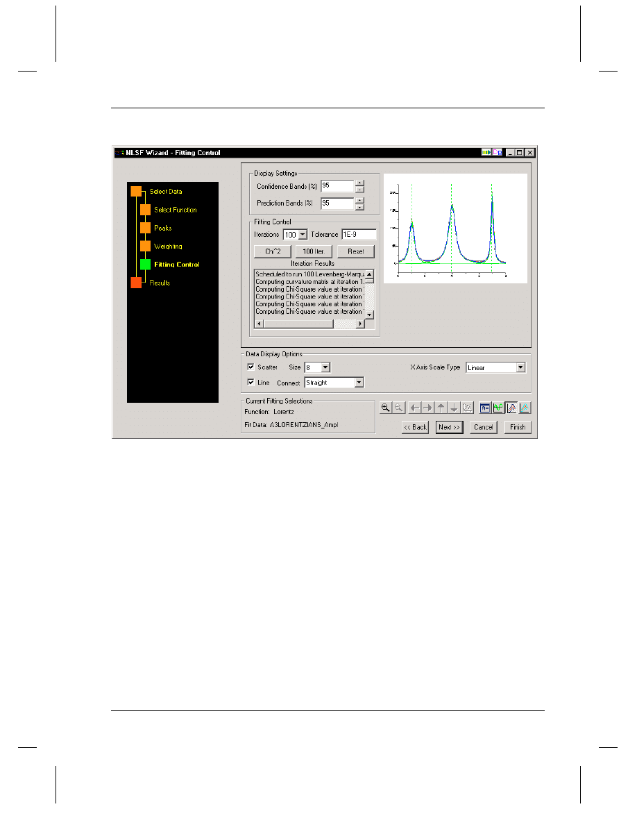
NLSF Wizard

Origin 7 provides a wizard for performing nonlinear least squares fitting.
The NLSF wizard is easier to use than the advanced fitting tool (NLSF),
as it steps you through the fitting process. The wizard provides only the
most frequently used fitting options. For complete fitting options, open
the NLSF.
To open the NLSF Wizard, select Analysis:Nonlinear Curve
Fit:Fitting Wizard.

Chapter 3, What's New in Version 7

Ease-of-Use

•

Figure 8: The NLSF Wizard

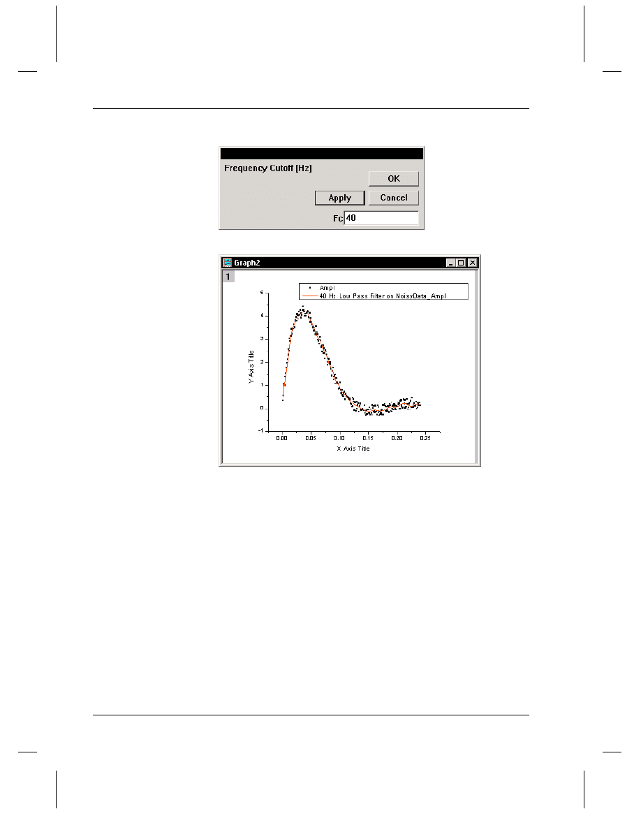
Analysis Apply Button

The following analysis routines now have an Apply button available in
their respective dialog boxes. When the Apply button is clicked, the
interim results display in the graph. The dialog box remains open and is
available for further changes. Each time you change a dialog box setting
and click Apply, the results update in the graph. The results are not
finalized until you click OK.
=> The following graph menu commands have an Apply button:
Analysis:Smoothing:Savitzky-Golay, Adjacent Averaging, and FFT
Filter
Analysis:FFT Filter:Low Pass, High Pass, Band Pass, and Band
Block
Analysis:Interpolate/Extrapolate
=> The following worksheet menu commands have an Apply button:
Statistics:Descriptive Statistics:Frequency Count

Chapter 3, What's New in Version 7

•

Ease-of-Use

Figure 9: 40 Hz Low Pass Filter Applied

Data Import and Handling

Thermo Galactic SPC

You can now import Thermo Galactic SPC data files into Origin by
selecting File:Import:Galactic (SPC). Origin supports both single and
multiple arrays.
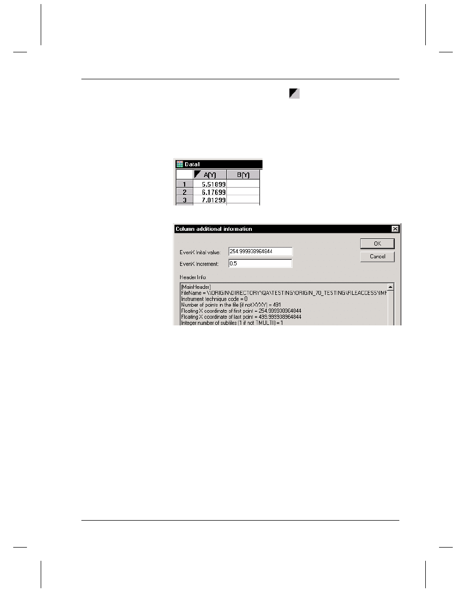
=> If the data file contains an array of X values, then Origin assigns
those values to an X column.
=> If the initial X value and the increment are stored in the header, then
Origin creates a hidden X column with the correct starting value and
increment. To view this information in Origin, perform one of the
following operations:

Chapter 3, What's New in Version 7

Ease-of-Use

•

1) Double-click on the black triangle

located in the upper-left corner

of the column heading. This action opens the Column Additional
Information dialog box. You can modify the starting X value and
increment in the associated text boxes.

Figure 10: Reviewing the Starting X Value and Increment

2) Click on the column heading to select the column and then select
Format:Set Worksheet X. This menu command also opens a dialog
box for modifying the starting X value and increment.
To view the hidden X column, select View:Show X Column.

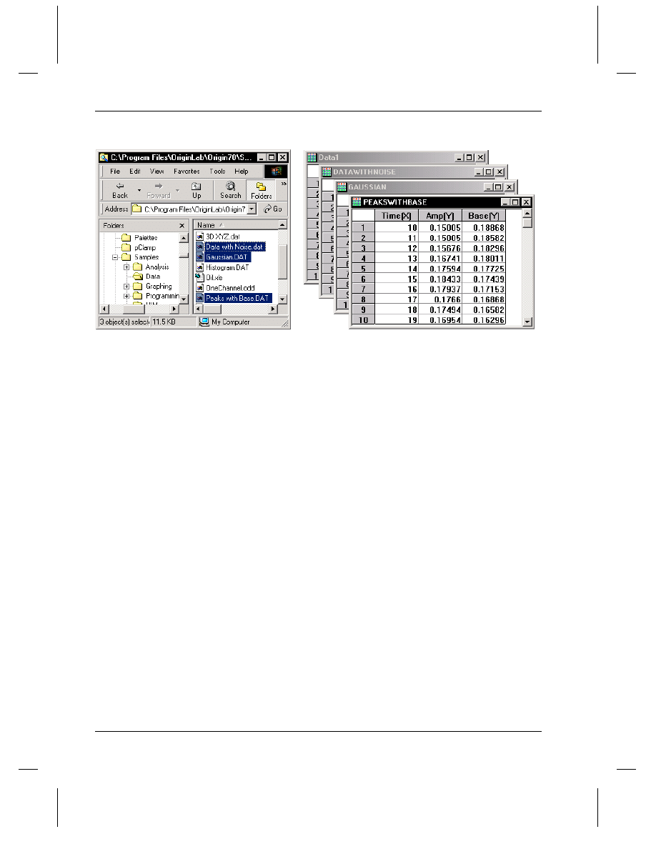
Drag-and-Drop

You can drag-and-drop ASCII, SigmaPlot, Minitab, and Thermo Galactic
SPC files into Origin. Once you have selected the file in Windows
Explorer, if Origin isn't currently open you can drag the file onto your
Origin desktop icon. If Origin is already open, you can drag the file over
the Origin taskbar button and hold there until Origin becomes active.
Then continue dragging and drop the file into the Origin workspace.
You can drop the data files into existing worksheets or graphs, or you can
drop into a blank location of the workspace to import into a new
worksheet for a single file, or multiple worksheets for multiple files.

Chapter 3, What's New in Version 7

•

Ease-of-Use

Figure 11: Dragging Data Files Into Origin

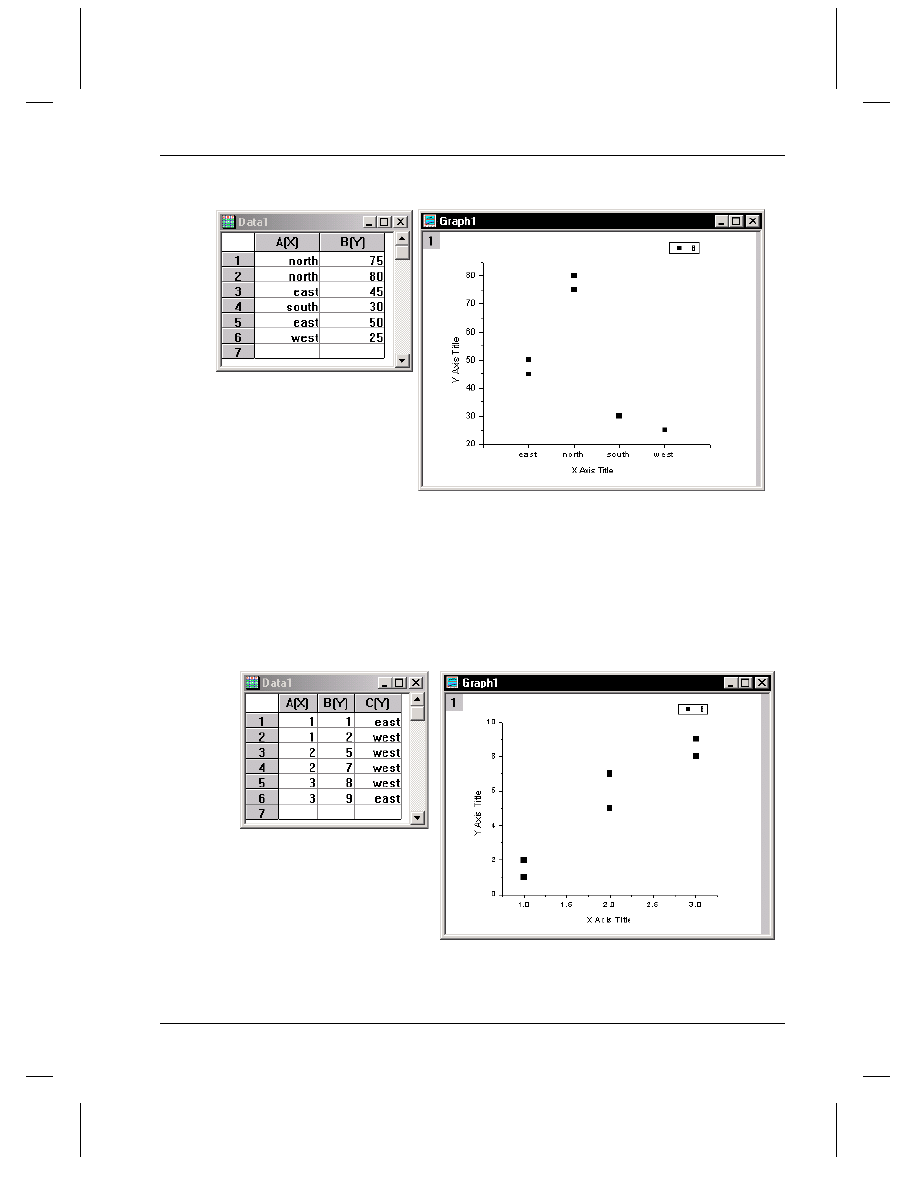
Categorical Data Support

Origin 7 supports plotting categorical data in both X and Y columns.
Before plotting categorical data, you must set the column to Categorical
by highlighting the column and selecting Column:Set as Categorical.
=> When you plot a Categorical X column and one or more associated Y
columns, Origin creates a graph with the X categories as X axis tick
labels. These tick labels are organized alphabetically (categories starting
with numeric values are first) and then evenly spaced across the axis.
The Y data is plotted using the associated X tick values.

Chapter 3, What's New in Version 7

Ease-of-Use

•

Figure 12: Plotting Categorical X Data

=> If your worksheet contains a Categorical Y column, then you can
map this categorical data to your data plots, displaying categories of data
using the same symbol shape, color, size, or other plot attribute.
For example, in the following figure, the A(X) and B(Y) columns are
plotted using the Scatter template.

Figure 13: Plotting the A(X) and B(Y) Columns

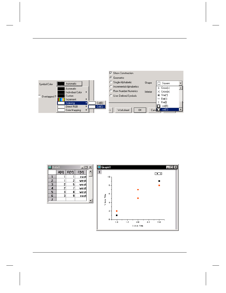
To display categories of data (east, west) using the same symbol shape
and color, open the Symbol tab of the Plot Details dialog box and edit the

Chapter 3, What's New in Version 7

•

Ease-of-Use

Symbol Color and Shape drop-down lists as shown in the following
figure. In this example the colors for each category will be indexed from
the color list.

Figure 14: Mapping the Symbol Color and Shape to Column C

The resultant graph displays the data using the column C categories for
both the symbol color and shape. To do this, Origin alphabetizes the
categories (categories starting with numeric values are first). Because
color indexing was selected, Origin assigns the first category the first
color in the color list, the second category the second color, etc. Origin
performs this same alphabetic assignment for all other mapped plot
attributes.

Figure 15: The Resultant Graph

Chapter 3, What's New in Version 7

Analysis Power

•

Analysis Power

New Graph Types

Image Graph

Origin 7 provides enhanced support for importing, viewing, and plotting
raster graphic images. To import a gray scale, 8-bit color or higher
resolution color image into the active matrix, select File:Import Image.
When you first import the image, Origin displays a device independent
bitmap (DIB) of the image in the matrix.
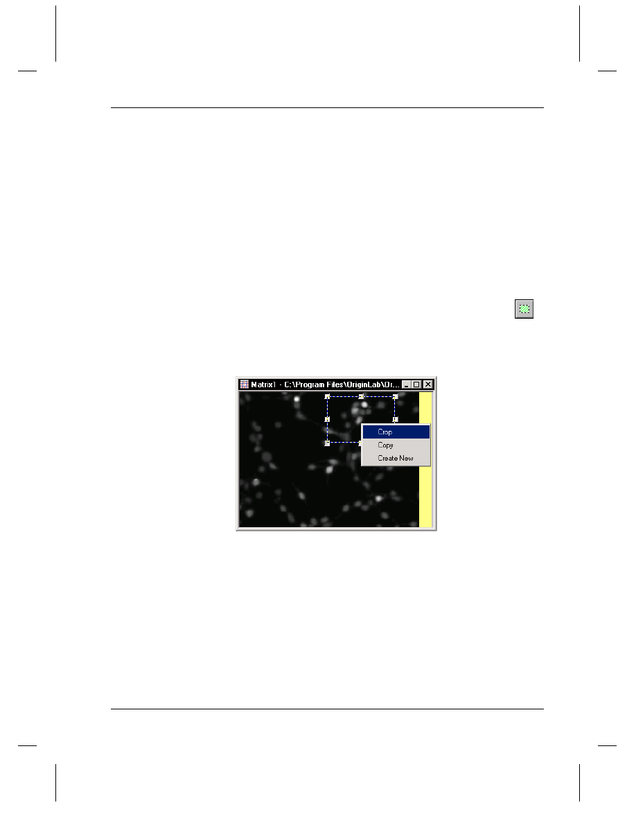
If you are only interested in a region of the image, you can select a region

of the DIB using the Rectangle Tool (in "region of interest mode")
on the Tools toolbar.

Figure 16: Selecting a Region of Interest

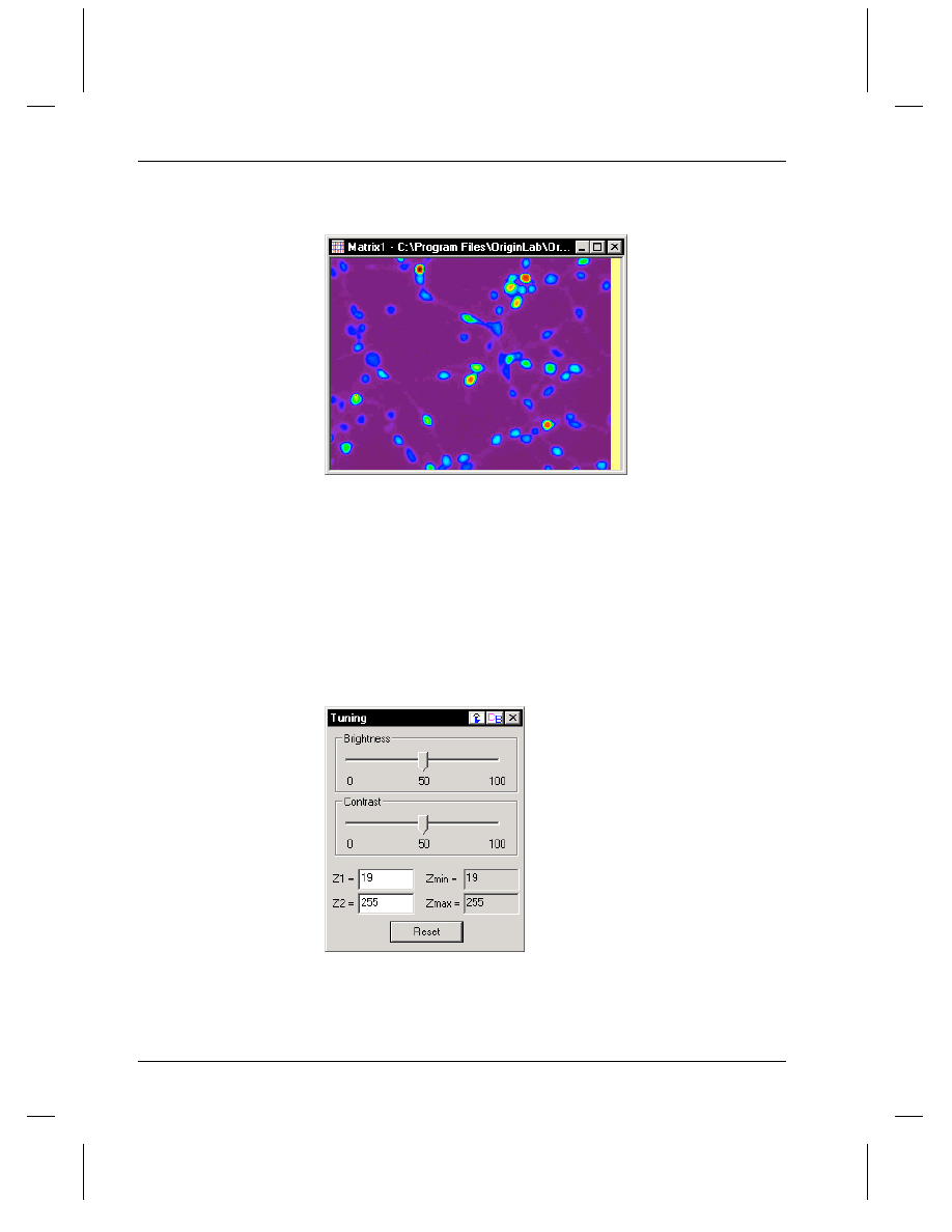
You can also view the image using a built-in or user supplied color
palette. Viewing the image using a specified color palette may clarify
regions of the image. To view the image using a color palette, you must
first convert the DIB to matrix data. To do this, select Image:Convert
to Gray + Data. Origin converts each pixel to an RGB value and then
assigns the corresponding matrix cell an index number to a gray scale
palette, based on the RGB value of the pixel. To display the image using
a palette other than gray scale, select Image:Palette:PaletteSelection.

Chapter 3, What's New in Version 7

•

Analysis Power

Figure 17: Viewing the Image Using a Built-in Palette for Improved
Clarity

When viewing the image from a palette, Origin maps each cell's index
value to a color in the selected palette. Thus, the image's full matrix Z
value range is mapped to the palette. You can adjust the brightness and
the contrast of the image using the Tuning tool. To open this tool, select
Image:Tuning. When you adjust the Contrast slider, you are increasing
or decreasing the Z value range that is mapped to the palette. When you
adjust the Brightness slider, you are shifting the range of Z values that
are mapped to the palette.

Figure 18: Adjusting the Brightness and Contrast of the Image

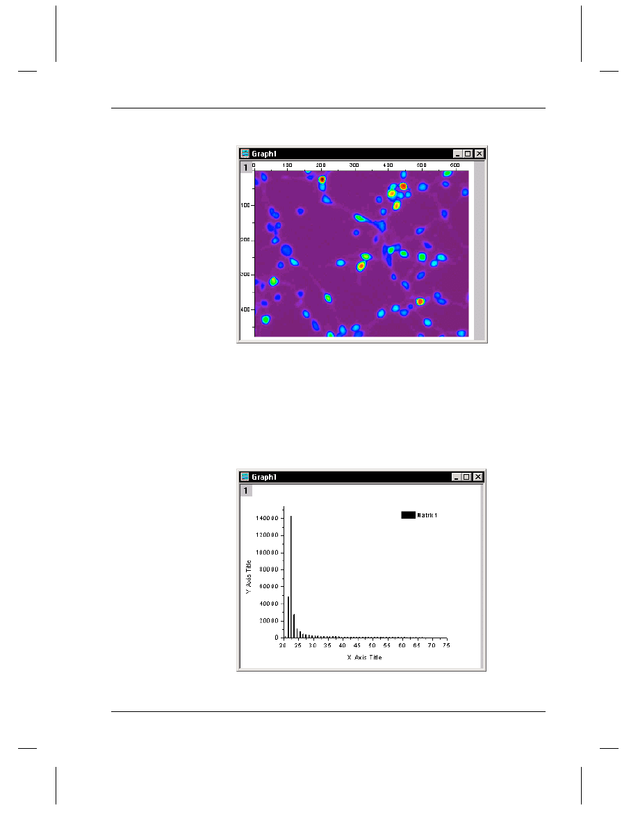
To plot the image into a graph window, select Plot:Image Plot.

Chapter 3, What's New in Version 7

Analysis Power

•

Figure 19: Plotting the Image into a Graph

Image Histogram

After importing a raster graphic image into a matrix, Origin can create a
histogram of the intensity values in the image. To plot a histogram from
the image in the matrix, select Plot:Histogram.

Figure 20: Example Image Histogram

Chapter 3, What's New in Version 7

•

Analysis Power

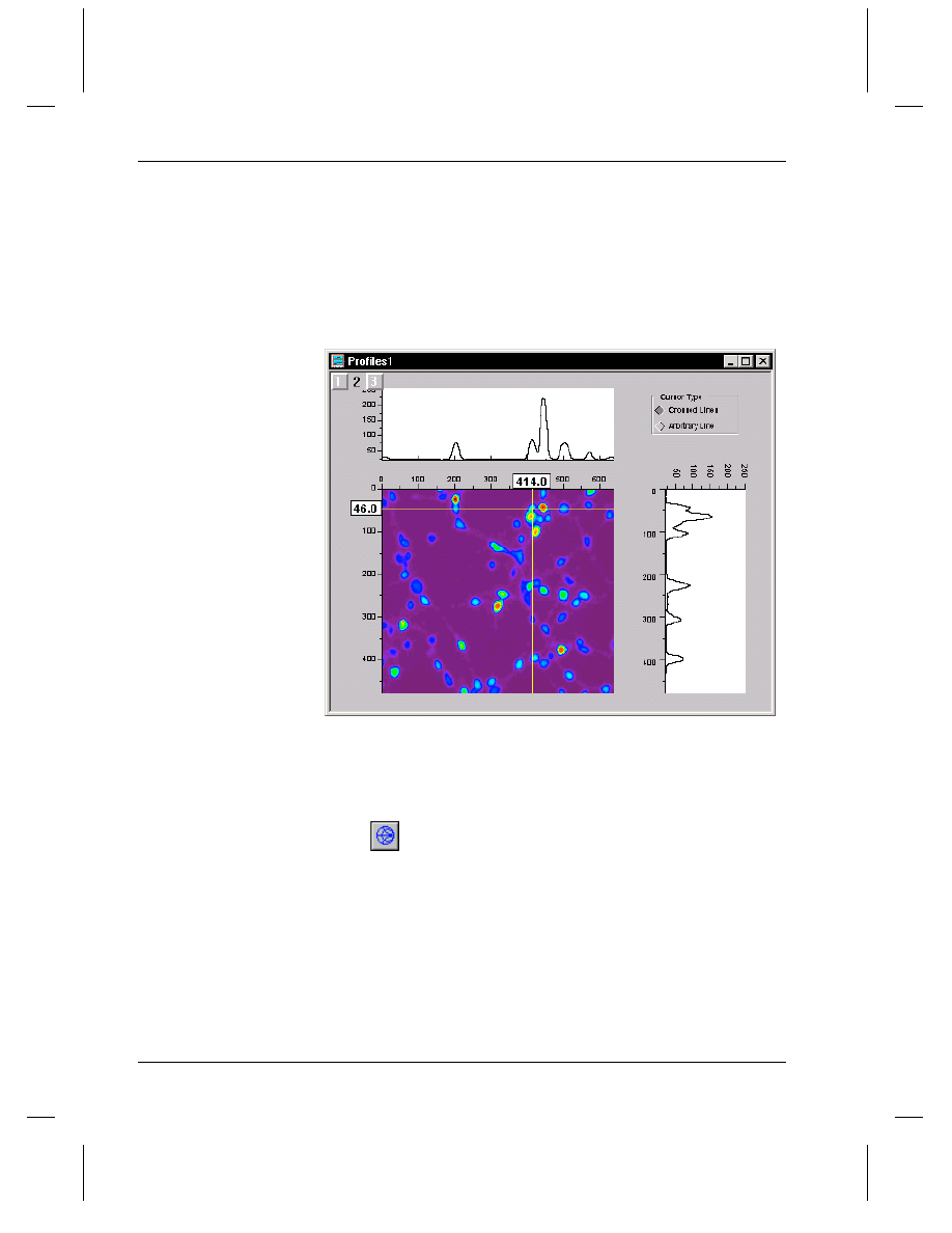
Image Profiling

Matrix images can also be plotted using a graph template that includes X
and Y projections. To plot to this template, select Plot:Profiles. You
can drag the lines to view different X and Y projections. You can also
view the projections using an arbitrary line.

Figure 21: Viewing the Images X and Y Projections

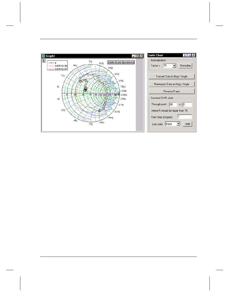
Smith Chart

You can now create Smith

Charts in Origin 7. To plot data using the

Smith Chart template, select Plot:Smith Chart or click the Smith Chart

button

on the 2D Graphs toolbar.

To customize the Smith Chart, edit the Plot Details and Axes dialog
boxes. Additionally, click the Smith Chart Operations button to open the
Smith Chart tool.

Chapter 3, What's New in Version 7

Analysis Power

•

Figure 22: Smith Chart with Operations Tool

Statistical Analysis

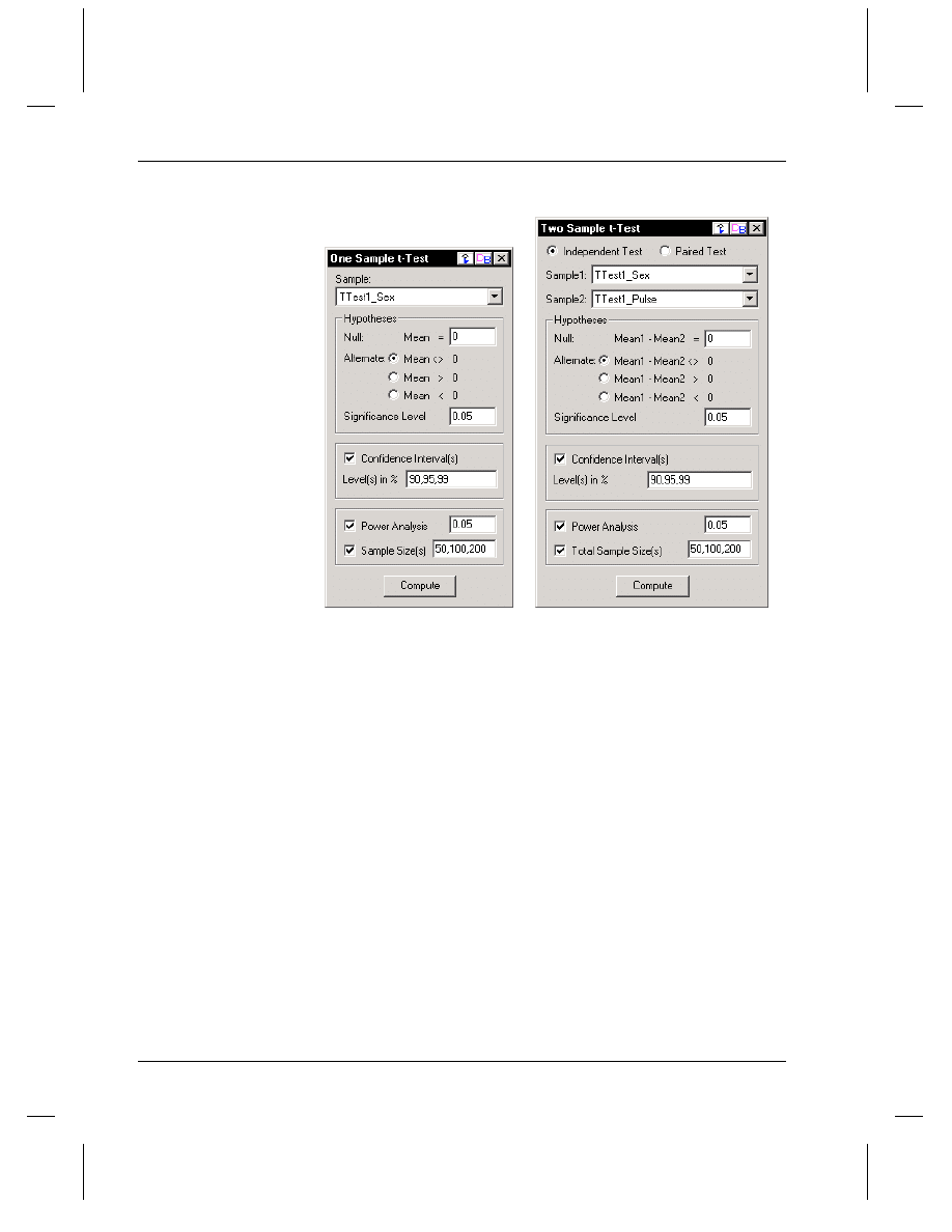
One / Two Sample t-Test

One and two sample t-Tests have been completely redesigned and
expanded in Origin 7. The following new features have been added:
=> You can now select new data sets, change settings, and re-compute
without having to re-open the dialog box each time.
=> Both one and two tailed tests can now be computed by selecting any
one of three Alternate Hypotheses.
=> Confidence intervals for a number of different confidence levels can
now be computed.
=> Actual Power can now be computed for any specified alpha level.
=> Hypothetical Power for a number of different sample sizes can now
be computed.
One and two sample t-Tests are available from the Statistics:Hypothesis
Testing menu.

Chapter 3, What's New in Version 7

•

Analysis Power

Figure 23: One and Two Sample t-Test Dialog Boxes

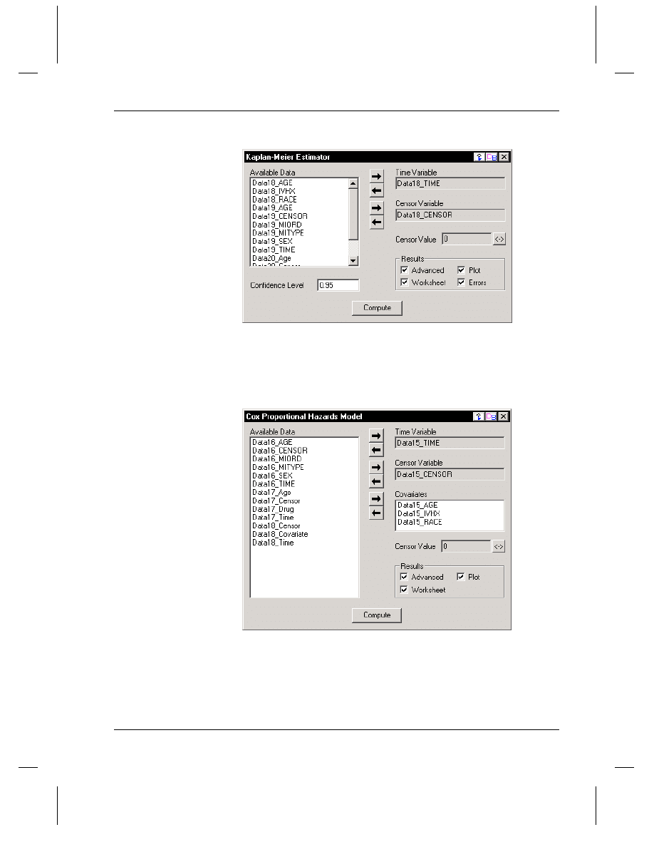
Survival Analysis

The Survival Analysis features are new in Origin 7. Two computations
are available:
=> Kaplan-Meier Product Limit Estimator
=> Cox Proportional Hazards Model
Both of these computations are used to estimate the survivorship function
which is the probability of survival to a given time based on a sample of
failure times.
To use the Kaplan-Meier estimator, select Statistics:Survival
Analysis:Kaplan-Meier Estimator.

Chapter 3, What's New in Version 7

Analysis Power

•

Figure 24: Kaplan-Meier Estimator Dialog Box

To use the Cox Proportional Hazards model, select Statistics:Survival
Analysis:Cox Proportional Hazards Model.

Figure 25: Cox Proportional Hazards Model Dialog Box

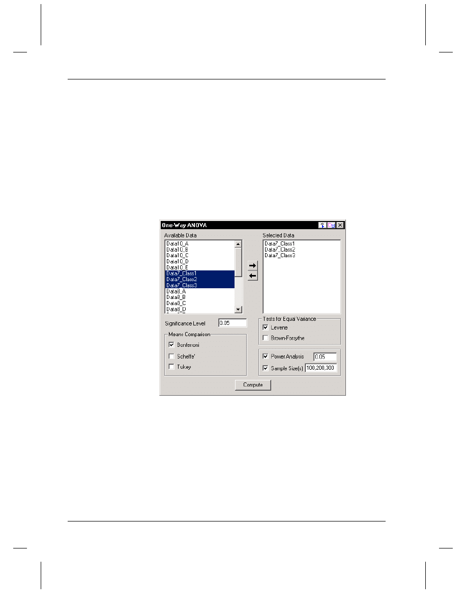
One-Way ANOVA

One-way ANOVA has been redesigned and expanded in Origin 7. The
following new features have been added:

Chapter 3, What's New in Version 7

•

Analysis Power

=> You can now select new data sets, change settings, and re-compute
without having to re-open the dialog box each time.
=> Non-contiguous column selection from any worksheet in the project.
=> Three different methods of Means Comparison (Bonferroni, Scheffé,
Tukey) can now be computed.
=> Two different Tests for Equal Variance (Levene, Brown-Forsythe)
can now be computed.
=> Actual Power can now be computed for any specified alpha level.
=> Hypothetical Power for a number of different sample sizes can now
be computed.
One-way ANOVA is available from the Statistics:ANOVA menu.

Figure 26: One-way ANOVA Dialog Box

Two-Way ANOVA

Two-way ANOVA evaluates the effect of two independent factors on a
measured response and whether or not there is an interaction between the
two factors. This feature is new in Origin 7 and will support the
following new computations:
=> You can select new data sets, change settings, and re-compute
without having to re-open the dialog box each time.
=> Non-contiguous column selection from any worksheet in the project,
and the ability to group levels of each factor either by classification

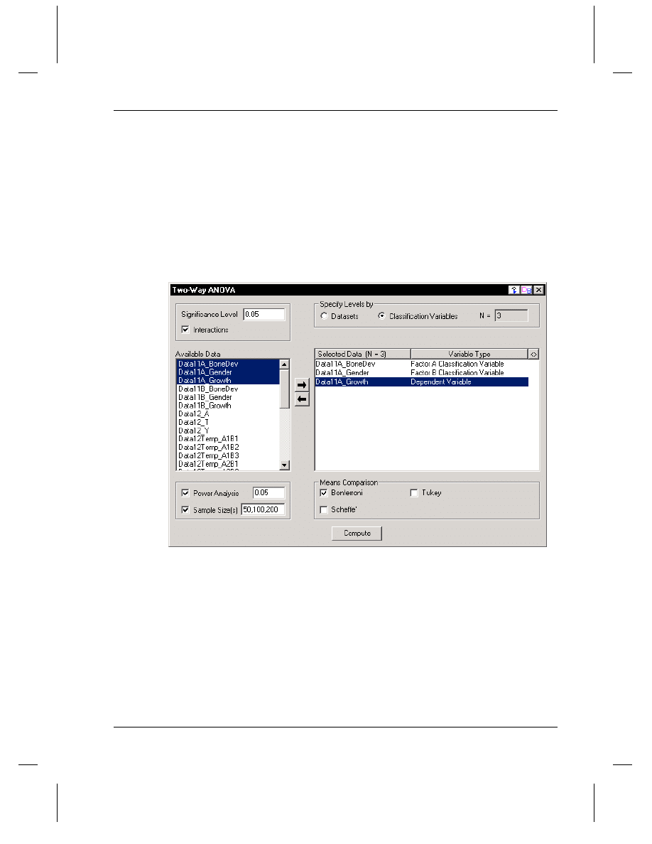
Chapter 3, What's New in Version 7

Analysis Power

•

variables or by data set.
=> Three different methods of Means Comparison (Bonferroni, Scheffé,
Tukey) can be computed.
=> A computation that determines whether or not there are any
interactions between the two factors.
=> Actual Power can be computed for any specified alpha level.
=> Hypothetical Power for a multiple number of different sample sizes
can be computed.
Two-way ANOVA is available from the Statistics:ANOVA menu.

Figure 27: Two-way ANOVA Dialog Box

Normality Test

You can now perform a Shapiro-Wilk normality test by selecting one or
more columns of data and then selecting Statistics:Descriptive
Statistics:Normality Test (Shapiro-Wilk). This test detects departures
from normality without requiring that the mean or variance of the
hypothesized normal distribution be specified in advance. For each
selected data set, the sample size N, the Shapiro-Wilk statistic W and its
significance level for testing normality P(W), and the decision rule are
output to the Results Log.

Chapter 3, What's New in Version 7

•

Analysis Power

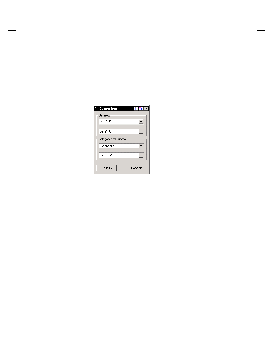
Fit Comparison

A new Fit Comparison tool is available by selecting Tools:Fit
Comparison. This tool compares two data sets by fitting the same
function to the data. It then uses an F-test to determine whether the two
data sets are significantly different from each other. The results are
output to the Results Log.

Figure 28: Fit Comparison Tool

Programming

Origin C

Origin 7 introduces a new programming language called Origin C.
Origin C supports a nearly complete ANSI C language syntax and a
subset of C++ features including internal and DLL-extended classes.
Furthermore, Origin C is "Origin aware". This means that Origin objects
such as worksheets and graphs are mapped in Origin C, allowing direct
manipulation of these objects and their properties from Origin C.
Typical programming routines in Origin include the following:
=> Adding functionality to Origin by creating new importing, analysis,
graphing, and exporting routines.
=> Automating the work you do in Origin.
=> Performing simulations in Origin, with live feedback.
To learn more about programming using Origin C, select
Help:Programming:Program Guide from the Origin menu.
Additionally, sample Origin projects and associated source files are
included in the \Samples\Programming subfolders.

Chapter 3, What's New in Version 7

Analysis Power

•

Code Builder

Code Builder is Origin's integrated development environment. To open

Code Builder, click the Code Builder button

on the Standard

toolbar. Code Builder provides standard tools for writing, compiling,
and debugging your Origin C functions. Once an Origin C function is
compiled, the function becomes accessible from Origin.

NAG Numerical Library

Origin 7 includes the following Numerical Algorithms Group (NAG

)

function libraries:
a02 - Complex Arithmetic
c06 - Fourier Transforms
e01 - Interpolation
e02 - Curve and Surface Fitting
F - Linear Algebra
f06 - Linear Algebra Support Functions
g01 - Simple Calculations on Statistical Data
g02 - Correlation and Regression Analysis
g03 - Multivariate Methods
g04 - Analysis of Variance
g08 - Nonparametric Statistics
g11 - Contingency Table Analysis
g12 - Survival Analysis
s - Approximations of Special Functions
Many of these functions are called from built-in Origin routines.
However, you can also call any of these NAG functions from Origin C.
To learn more, review the sample Origin project files provided in the
\Samples\Programming\NAG ... folders.

Chapter 3, What's New in Version 7

•

Analysis Power

Chapter 4, Getting Started Using Origin

The Origin Workspace

•

Chapter 4, Getting Started Using

Origin

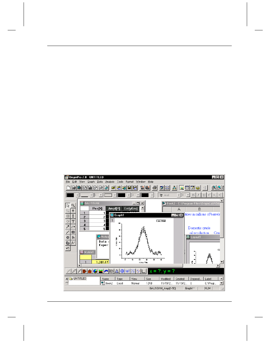
The Origin Workspace

When you start Origin, a new project opens displaying a worksheet
window in the workspace. The worksheet is one type of window
available in Origin. Origin also provides graph (including function
graph), layout page, Excel workbook, matrix, and notes windows.
Having various windows allows you to simultaneously view different
visual representations of your data - such as data in a worksheet versus a
graph - simplifying data manipulation and analysis.

Figure 1: The Origin Workspace and Supported Window Types

Chapter 4, Getting Started Using Origin

•

The Origin Workspace

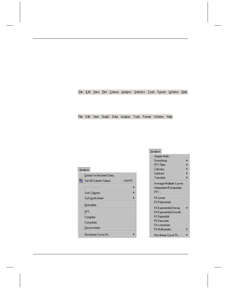
Menus and Menu Commands

Origin's menu bar provides commands to perform operations on the
active window and to perform general operations such as opening a Help
file or turning on the display of a toolbar. The menu bar changes as you
change the active window. For example, the following figures compare
the worksheet and graph menu bars.

Figure 2: The Worksheet Window Menu Bar

Figure 3: The Graph Window Menu Bar

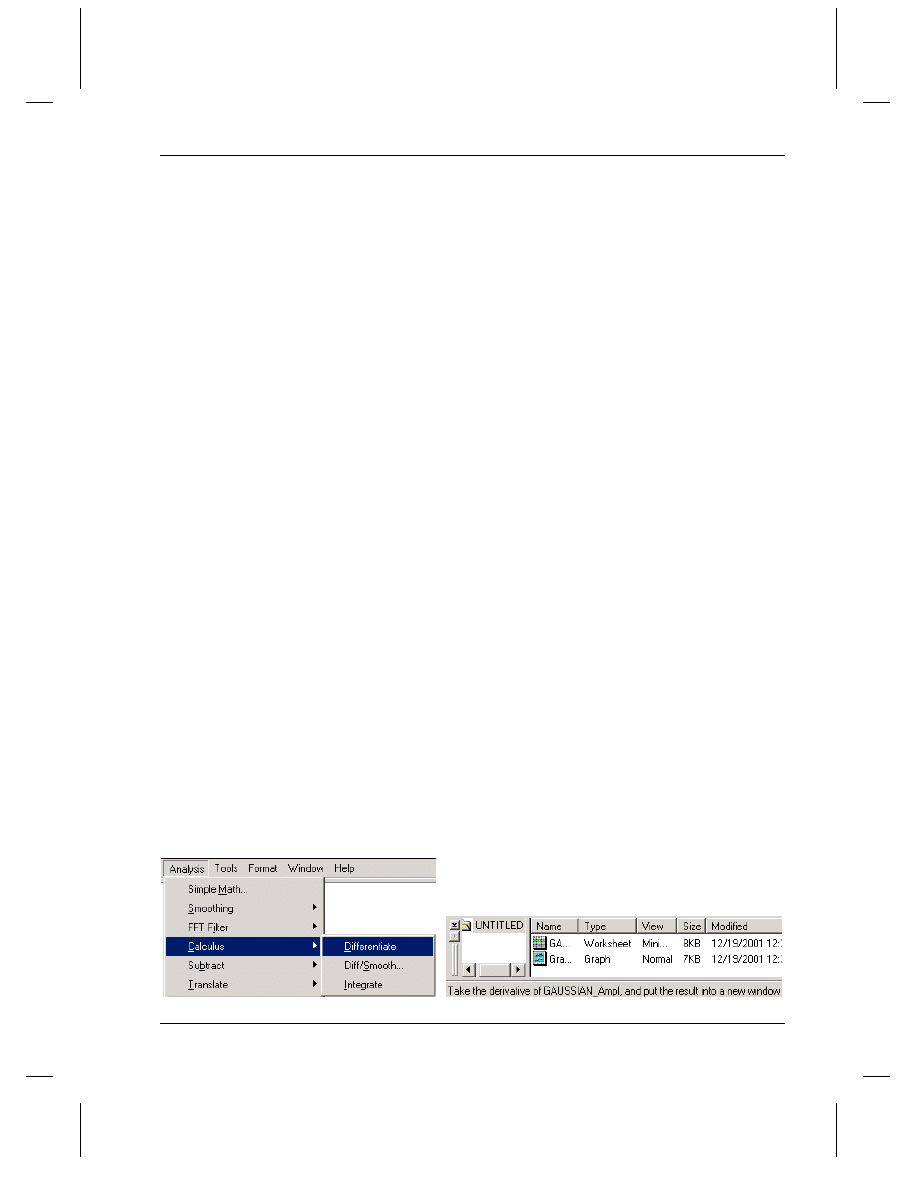
Menus are also sensitive to the active window. For example, the
following figure compares the worksheet and graph Analysis menus.

Figure 4: The Worksheet and Graph Analysis Menus

Chapter 4, Getting Started Using Origin

The Origin Workspace

•

Origin provides two menu "levels" which determine the number of menu
commands that are available. By default, Origin displays the "full
menu", which means that all available menu commands are provided.
However, Origin also offers a "short menu" level, which provides a
reduced set of menu commands for performing basic operations only. To
activate this reduced set of commands, select Format:Menu:Short
Menus. At any time you can re-activate the full set of commands by
selecting Format:Menu:Full Menus.
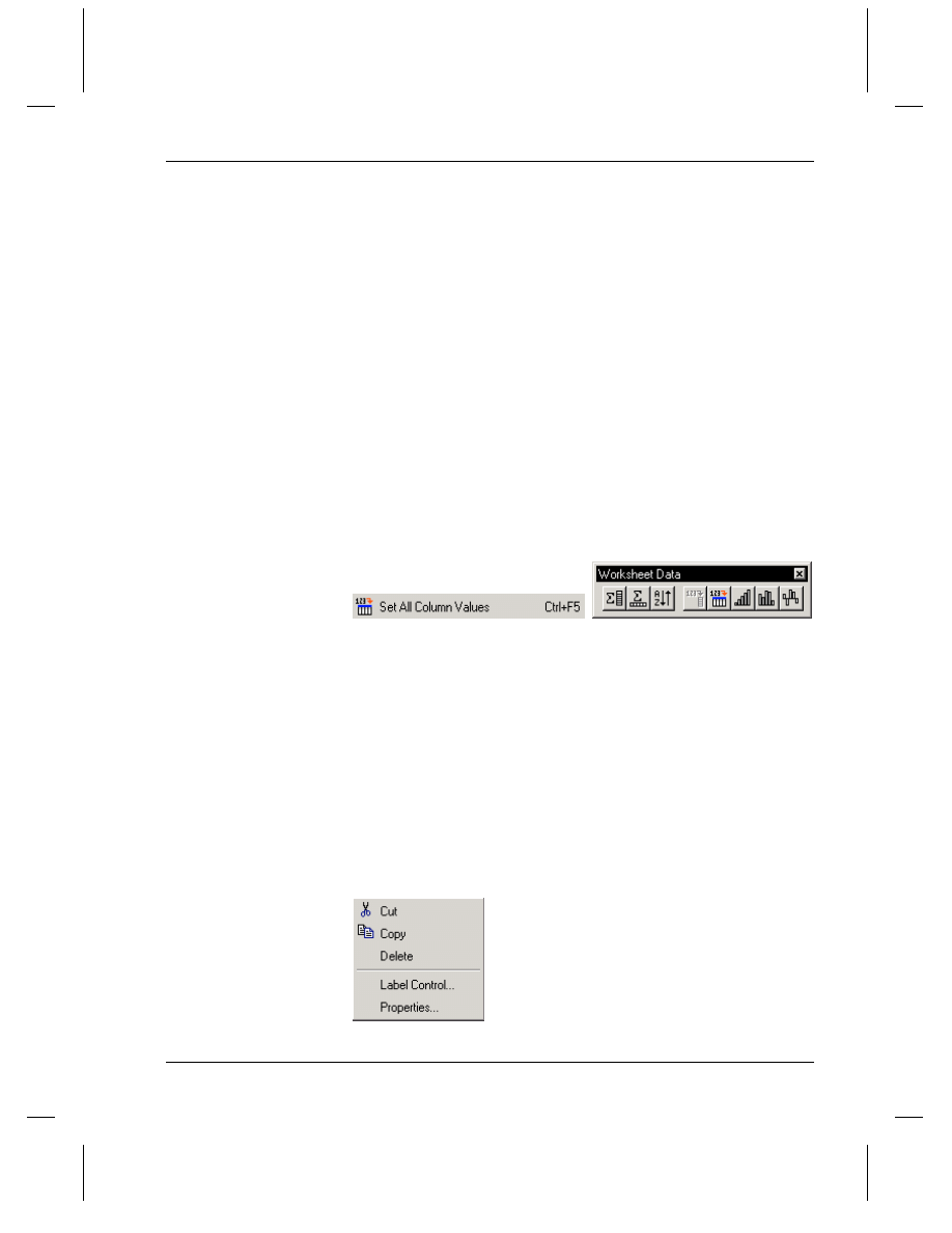
Some menu commands have shortcut keys associated with them. If
available, the shortcut key displays to the right of the menu command.
For example, when a worksheet window is active, you can press
CTRL+F5 to access Set All Column Values. (Note: You can't use a
shortcut key if the menu is open.)
Some menu commands also have bitmaps that display to the left of the
command. The bitmap indicates that the menu command also has toolbar
button access. To access the command from a toolbar, look for the
toolbar button represented by the command's bitmap.

Figure 5: Accessing a Command from a Toolbar

(To learn how to open additional toolbars, such as the Worksheet Data
toolbar, see "Toolbars" on page 48.)
To turn off the display of bitmaps in the menus, select Tools:Options to
open the Options dialog box. Select the Miscellaneous tab and then clear
the Display Bitmaps in Menus check box. After you click OK, you are
asked if you want to save this setting for future Origin sessions.
Many commands are also available from shortcut menus. To open a
shortcut menu, right-click on the object you want to perform an action
on. For example, if you right-click on a text label, the shortcut menu in
the following figure opens.

Figure 6: Opening a Shortcut Menu

Chapter 4, Getting Started Using Origin

•

The Origin Workspace

Toolbars

Origin provides toolbar buttons for frequently used menu commands. As
with menu commands, some toolbars are only available when a particular
window (for example, a worksheet) is active. Additionally, a toolbar that
is available for multiple window types may contain buttons that are
window-sensitive.
When you position the mouse pointer over a toolbar button, a view box
opens displaying the button name, which indicates its purpose. A more
detailed description also displays in the status bar.

Figure 7: Viewing a Button's Name and Purpose

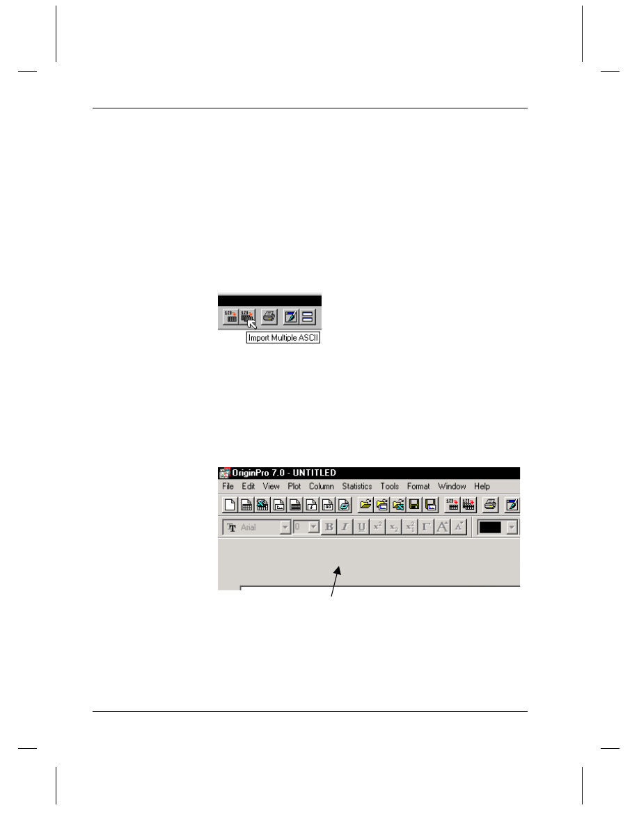
If you open Excel workbooks in Origin, when you change the active
window from an Excel workbook to any other window type (for
example, a worksheet), or when you close an Excel workbook, the
toolbar region displays a blank area where the Excel toolbars were
located (see the following figure).

Figure 8: Blank Area in the Toolbar Region

Blank area where the Excel toolbars were located.

Chapter 4, Getting Started Using Origin

The Origin Workspace

•

To open the Options
dialog box when an
Excel workbook is
active, select
Window:Origin
Options.

This area is called a toolbar spacer. To hide the toolbar spacer, right-
click in the region and select Hide Toolbar Spacer from the shortcut
menu. When you re-activate the Excel workbook window or re-open a
workbook, Origin will automatically show the toolbar spacer with the
Excel toolbars. (To prevent Origin from using the toolbar spacer, select
Tools:Options to open the Options dialog box. Select the
Miscellaneous tab and then clear the Use Toolbar Spacer check box.
After you click OK, you are asked if you want to save this setting for
future Origin sessions.)

When you first start Origin, the following toolbars are available:
Standard, Graph, Format, Style, Tools, and 2D Graphs.

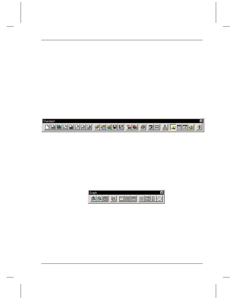
Figure 9: The Standard Toolbar

The Standard toolbar provides buttons for opening, saving, and creating
new projects and windows, and for importing ASCII data. It also
provides buttons for general window operations such as printing,
duplicating, and refreshing windows. The Standard toolbar provides
buttons for opening Project Explorer, the Results Log, the Script
window, and Code Builder. A button is provided for custom
programming. A button is also provided for adding a column to the
worksheet.

Figure 10: The Graph Toolbar

The Graph toolbar is available when a graph or layout page is active. It
provides buttons to zoom in and out and to rescale axes to show all the
data. It provides buttons to display data plots in multiple layers, display
layers in multiple windows, and to merge windows. Labeling buttons are
available for legends and a time/date stamp.

Chapter 4, Getting Started Using Origin

•

The Origin Workspace

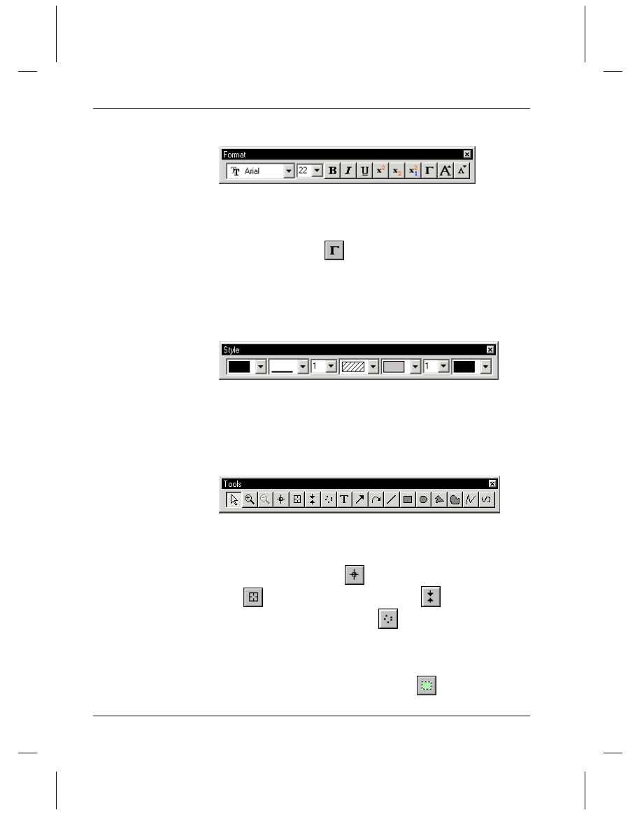
Figure 11: The Format Toolbar

The Format toolbar is available when a text label is active. This toolbar
provides text formatting buttons. Color control is available from the
Style toolbar.

Note: The Greek button

uses the Symbol font set. To associate the

button with a different font set, select Tools:Options to open the Options
dialog box. Select the Text Fonts tab and then select the desired font set
from the Greek drop-down list.

Figure 12: The Style Toolbar

The Style toolbar is available when a text label or other annotation is
selected. It provides buttons to set the line and fill color, style, and point
size.

Figure 13: The Tools Toolbar

The Tools toolbar provides text, arrow, line, and other annotation
buttons. It also provides buttons to enlarge a region of a graph. The
Tools toolbar also provides buttons to read the XY (and Z, if 3D or

contour) location on the page

, and the XY (and Z) location of a data

point

. You can also define a range of data

. Furthermore, a

button is provided to draw a data plot

For more information on the Screen Reader, Data Reader, and Data
Marker buttons, see "Tutorial 2, Exploring Your Data".
Note: If you are viewing an image in a matrix, you can display the

Rectangle tool in the "region of interest" mode

. The region of

Chapter 4, Getting Started Using Origin

The Origin Workspace

•

interest mode allows you to select a region of the image to crop, copy, or
duplicate. The region of interest mode is controlled from the
Tools:Show Tools as ROI menu command.

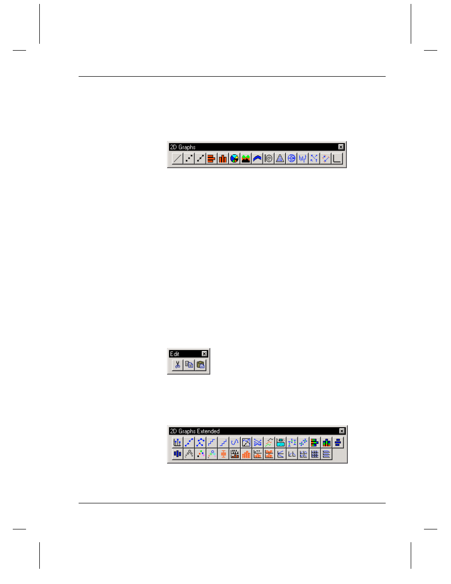
Figure 14: The 2D Graphs Toolbar

The 2D Graphs toolbar is available when a worksheet, Excel workbook,
or graph window is active. It provides buttons for the common 2D graph
templates, and for accessing a custom graph template.
=> When a worksheet or Excel workbook is active, first select the data
that you want to plot and then click the button on the 2D Graphs toolbar
to plot your data.
=> When a graph window is active, you can change the graph type (for
example, from scatter to column) for the active data plot. To activate a
data plot, select the data plot from the Data menu. Then click the button
on the 2D Graphs toolbar to change the graph type.

In addition to these default toolbars, you can open the following
additional toolbars. To do this, select View:Toolbars to open the
Customize Toolbar dialog box. Then select the desired toolbar from the
Toolbars tab.

Figure 15: The Edit Toolbar

The Edit toolbar provides cut, copy, and paste buttons.

Figure 16: The 2D Graphs Extended Toolbar

The 2D Graphs Extended toolbar is available when a worksheet, Excel
workbook, or graph window is active. It provides buttons for the

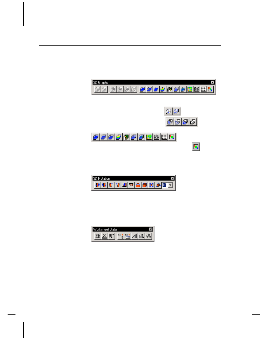
Chapter 4, Getting Started Using Origin

•

The Origin Workspace

additional 2D graph templates not accessible from the 2D Graphs toolbar.

Figure 17: The 3D Graphs Toolbar

The 3D Graphs toolbar is available when a worksheet, Excel workbook,

or matrix is active. The first two buttons

are available for

plotting XYZ data. The next four buttons

are

available for plotting XYY data. The remaining buttons

are available for

plotting matrices. The last button, the Image Plot button

, is

available for plotting images.

Figure 18: The 3D Rotation Toolbar

The 3D Rotation toolbar is available when a 3D graph is active. This
toolbar provides buttons to rotate the graph and change the perspective.

Figure 19: The Worksheet Data Toolbar

The Worksheet Data toolbar is available when a worksheet is active.
This toolbar provides buttons to perform statistics on columns or rows of
data, sort, use functions to set column values or mathematically
transform values, update these column values, and fill columns with row
numbers or random numbers.

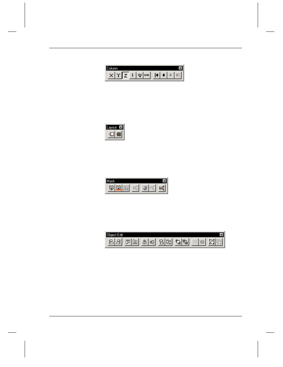
Chapter 4, Getting Started Using Origin

The Origin Workspace

•

Figure 20: The Column Toolbar

The Column toolbar is available when a worksheet column is selected. It
provides buttons to set the column plotting designation and to move
columns.

Figure 21: The Layout Toolbar

The Layout toolbar is available when a layout page is active. It provides
buttons to add pictures of graphs or worksheets to the layout page.

Figure 22: The Mask Toolbar

The Mask toolbar is available when a worksheet or graph is active. This
toolbar provides buttons to mask data from analysis.

Figure 23: The Object Edit Toolbar

The Object Edit toolbar is available when one or more annotation objects
are selected in the active window, or when more than one picture is
selected in a layout page. The toolbar provides buttons to align the
selected objects/pictures, and to change the drawing order of the
objects/pictures. Buttons are provided to group objects so that you can
move or align the group. Additionally, buttons are provided to change
the drawing order of objects relative to data plots.

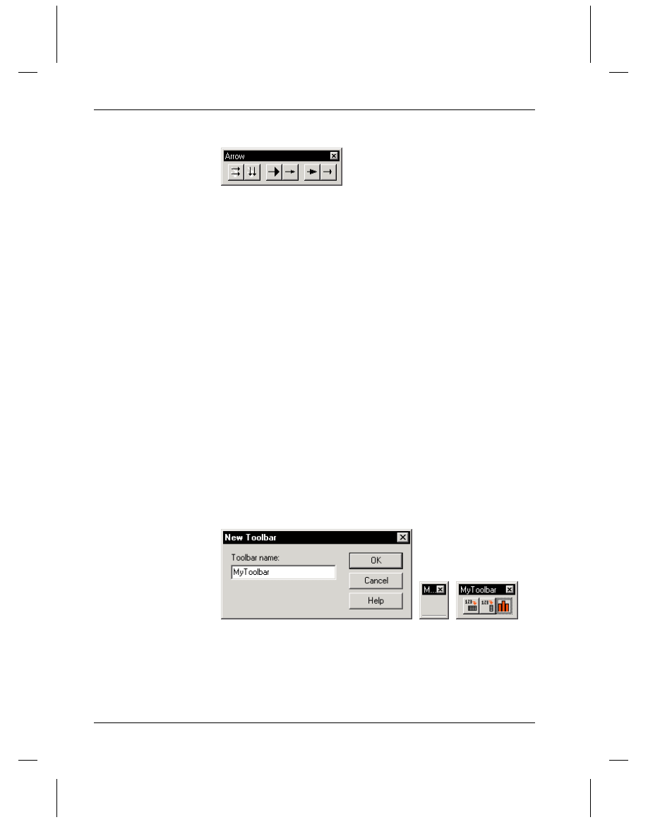
Chapter 4, Getting Started Using Origin

•

The Origin Workspace

Figure 24: The Arrow Toolbar

The Arrow toolbar is available when one or more lines or arrows are
selected. This toolbar provides buttons to align multiple lines/arrows,
and to customize the arrow head.

In addition to adding Origin's default toolbars to your workspace, you
can add and remove buttons from any of the default toolbars, or create
new toolbars containing a single button or a combination of buttons from
the default toolbars.
To add and remove buttons from any of Origin's default toolbars, select
View:Toolbars to enter the toolbar editing mode. You can now drag
toolbar buttons between toolbars. To remove a button from a toolbar,
drag the button off the toolbar (not on to another toolbar) and release the
mouse button. To add a button to a toolbar, select the Button Groups tab
on the Customize Toolbar dialog box. From the Groups list box, select
the toolbar which displays the button by default. Then drag the desired
button onto any of the toolbars.
To create a new toolbar, you can drag a button into the workspace or into
the toolbar region (not on to another toolbar). Alternatively, click New
on the Toolbars tab of the Customize Toolbar dialog box. Type the
desired name in the New Toolbar dialog box and click OK. Now select
the Button Groups tab and drag the desired buttons onto the new toolbar.

Figure 25: Creating a New Toolbar

Window Types

Origin provides a number of window types for viewing, analyzing, and
presenting your data. These windows include worksheet, matrix, Excel

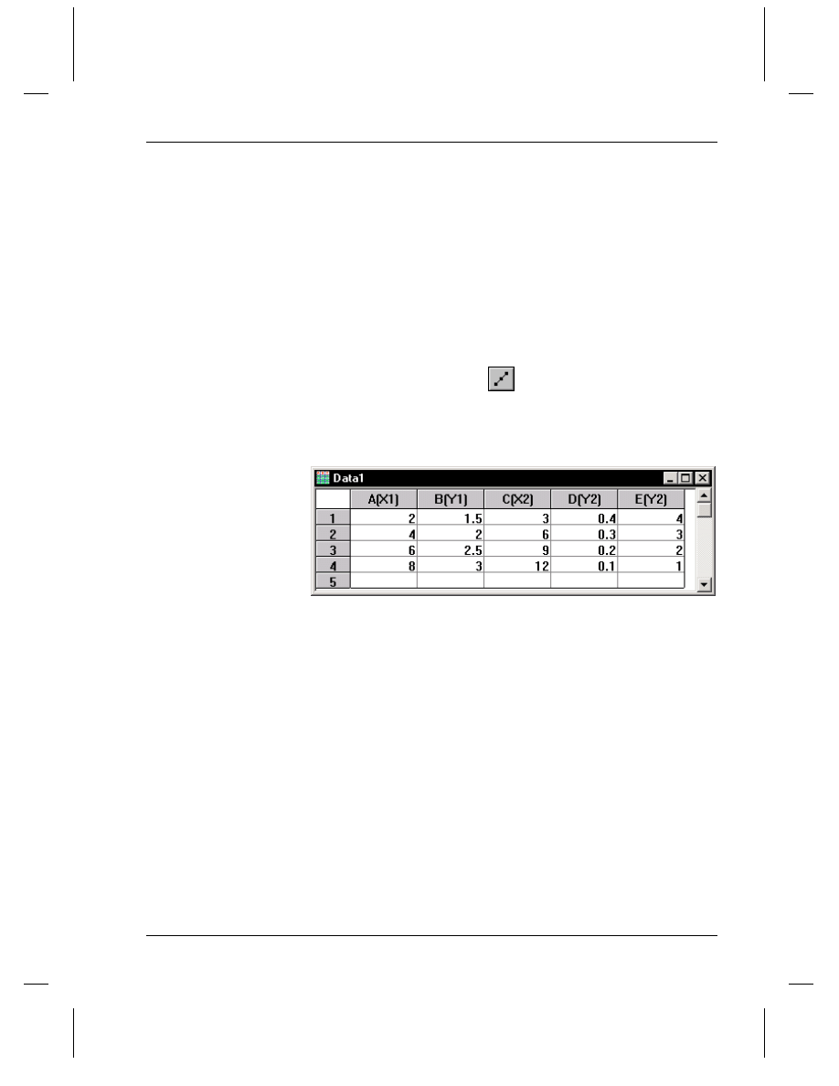
Chapter 4, Getting Started Using Origin

The Origin Workspace

•

workbook, graph, layout page, and notes windows. The window type
that is currently active in the Origin workspace determines the menu bar
and toolbars that are available.

Worksheet Windows

A worksheet's primary function is to hold and organize the data that you
bring into Origin, and to provide tools for data manipulation, exploration,
statistics, analysis, and plotting.
The columns in a worksheet are related to one another by their plotting
designation (such as X and Y) and their location. The plotting
designation determines how the selected data will plot. For example, in
the following worksheet, if you select columns A through E and then

click the Line & Symbol button

on the 2D Graphs toolbar, columns

A and B, C and D, and C and E will plot as XY pairs.

Figure 26: Worksheet Column Plotting Designations

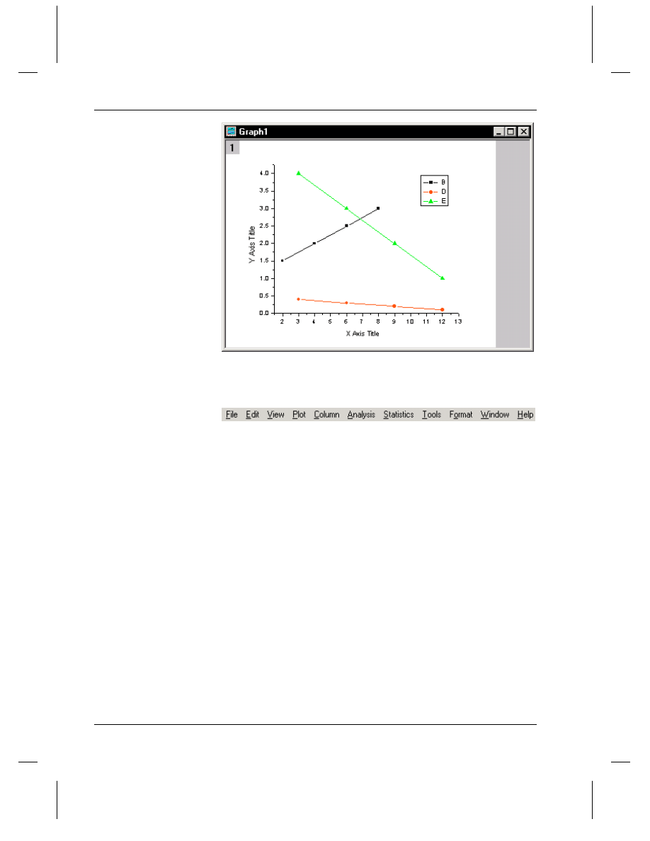
Chapter 4, Getting Started Using Origin

•

The Origin Workspace

Worksheet Menu Bar

The File menu provides Origin project and window commands that are
available independent of the active window. When a worksheet is active,
the File menu also provides commands to:
=> import and export data

Undo is available for
most worksheet
operations, but it is not
available for all Origin
operations.

The Edit menu provides cut, copy, paste, and undo commands that are
available independent of the active window. Additionally, a "button edit
mode" command is available for editing programmed labels. When a
worksheet is active, the Edit menu also provides commands to:
=> set the worksheet display range
=> convert the worksheet to a matrix
=> transpose and paste transpose

The View menu provides commands to control the display of the Project
Explorer window, toolbars, status bar, and Results Log. It also provides
a command to display a grid for aligning objects. These commands are
available independent of the active window. When a worksheet is active,
the View menu also provides commands to:
=> update a graph after changing the worksheet data
=> go to a specified worksheet row
=> show a hidden X column

Chapter 4, Getting Started Using Origin

The Origin Workspace

•

Select your data first.
Then select the Plot
menu command.

The Plot menu is only available when a worksheet, matrix, or Excel
workbook is active. The Plot menu provides commands to:
=> plot data into a specified graph template

Select your column first.
Then select the Column
menu command.

The Column menu is only available when a worksheet is active. This
menu provides commands to:
=> set the column's plotting designation
=> use functions to set column values or mathematically transform
values
=> add and move columns

The Analysis menu provides commands to:
=> extract data
=> sort data
=> normalize data
=> perform FFT-related operations
=> perform nonlinear curve fitting
The Statistics menu is only available when a worksheet is active. This
menu provides commands to:
=> perform a number of statistical tests on your data
The Tools menu command provides commands to set global preferences
in the Options dialog box, re-activate reminder messages, and pack
selected files into a single file to share with other Origin users. These
commands are available independent of the active window. When a
worksheet is active, the Tools menu also provides commands to:
=> associate LabTalk script with the worksheet
=> perform linear, polynomial, and sigmoidal fitting
=> compare two columns of data by fitting the same function to the data
The Format menu provides commands to display a reduced menu
structure in which only basic operations are available, to edit the name
and programming-related properties of a label, and to align objects to a
grid. These commands are available independent of the active window.
Additionally, the worksheet Format menu provides commands to:
=> set the worksheet or column display options
=> set incremental X values in a worksheet without a designated X
column
The Window menu provides commands to arrange the windows in the
workspace, open the Script window, activate a Project Explorer folder,
and activate a window in the workspace. These commands are available
independent of the active window.
The Help menu provides commands to open the Origin and
programming-related Help files, open a dialog box with tips on using
Origin, go to the OriginLab web site, and register your copy of Origin.
These commands are available independent of the active window.

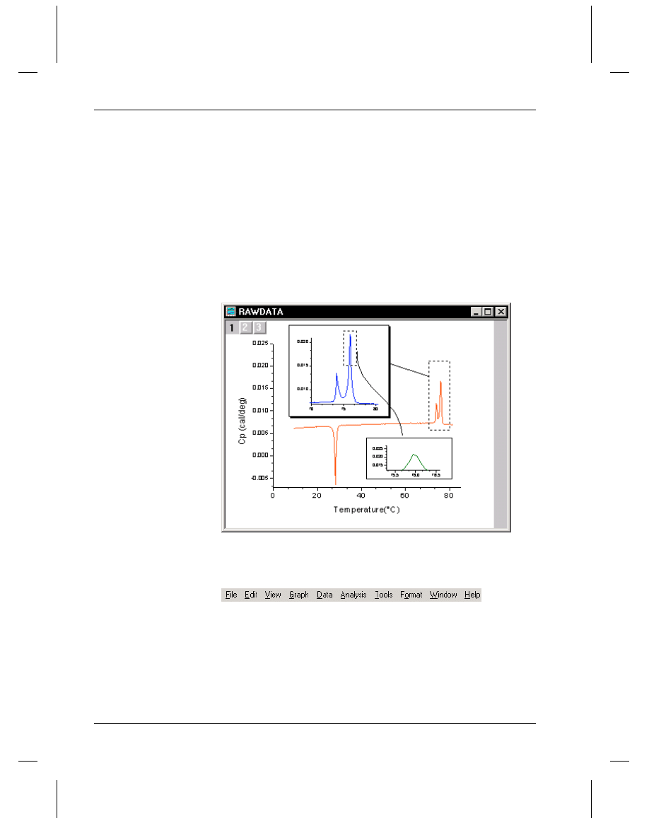
Chapter 4, Getting Started Using Origin

•

The Origin Workspace

Graph Windows

A graph window is a container and editor for creating graphs. Each
graph window contains a single editable page. The page serves as a
backdrop for the various graph objects, including layers, axes,
annotations, and data plots.
There are many ways to create graphs in Origin. The easiest method is to
select the worksheet data that you want to plot, and then select the
desired graph type from the Plot menu or from one of the plotting
toolbars. If you've already created a graph window, you can select and
drag data from a worksheet into the graph window.

Figure 27: A Graph with Multiple Layers

Graph Menu Bar

(See the Worksheet Menu Bar for commands that are available for all
window types.)

Chapter 4, Getting Started Using Origin

The Origin Workspace

•

When copying or when
exporting to a vector
image file, you can
control the graph size
from the Options
dialog box
(Tools:Options, Page
tab).

The File menu provides graph-specific commands to:
=> import ASCII data
=> import an image file
=> export the graph to an image file
The Edit menu provides graph-specific commands to:
=> copy a graph to the clipboard
=> add and arrange layers in the active graph
=> rotate the graph between landscape and portrait orientation
=> merge all the graph windows into one window

The View menu provides graph-specific commands to:
=> view the graph using the screen driver or active printer driver
=> zoom in and out of the graph
=> show or hide elements in the graph
=> resize the active graph layer so that it fills the page
=> resize the graph window so that it fills the screen

You can also drag data
from a worksheet or
Excel workbook into a
graph.

The Graph menu provides commands to:
=> add data to the graph, including error bars or a function
=> rescale the axes and exchange the X and Y axes
=> create a new legend or color scale for color mapped data
=> stack grouped data (most useful for column and bar charts)

You can open the Plot
Details dialog box for
a data set by pressing
CTRL and selecting it
from the list.

The Data menu provides graph-specific commands to:
=> set the display range
=> move and remove data points
The Data menu also lists the data sets that are plotted in the active
graph. The active data set is checked.

The Analysis menu provides graph-specific commands to:
=> perform linear and nonlinear fitting
=> perform math operations
=> smooth or filter the data
=> differentiate and integrate
=> perform a subtraction or translation
=> average curves
=> perform interpolation and extrapolation
=> perform an FFT
The Tools menu provides graph-specific commands to:
=> open analysis and fitting tools
=> open a tool for adding and arranging layers
=> compare two sets of data by fitting the same function to the data
The Format menu provides graph-specific commands to:
=> set the page, layer, data plot, and axes display options

Layout Page Windows

A layout page window is a “display panel” for graphs and worksheets
that have been created in other windows. You can add and arrange

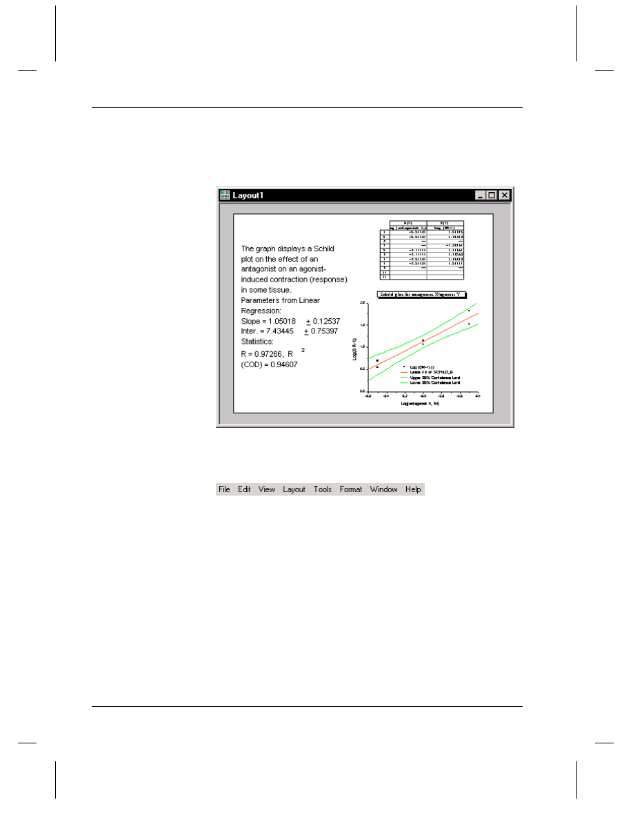
Chapter 4, Getting Started Using Origin

•

The Origin Workspace

worksheet and graph pictures in a layout page, as well as text and other
annotations.

Figure 28: A Layout Page Window

Layout Page Menu Bar

(See the Worksheet Menu Bar for commands that are available for all
window types.)

When copying or when
exporting to a vector
image file, you can
control the size from
the Options dialog box
(Tools:Options, Page
tab).

The File menu provides layout page-specific commands to:
=> import an image file
=> export the layout page to an image file
The Edit menu provides layout page-specific commands to:
=> copy a layout page to the clipboard
=> rotate the layout page between landscape and portrait orientation

The View menu provides layout page-specific commands to:
=> view the layout page using the screen driver or active printer driver
=> zoom in and out of the layout page
=> show master page items in the layout page

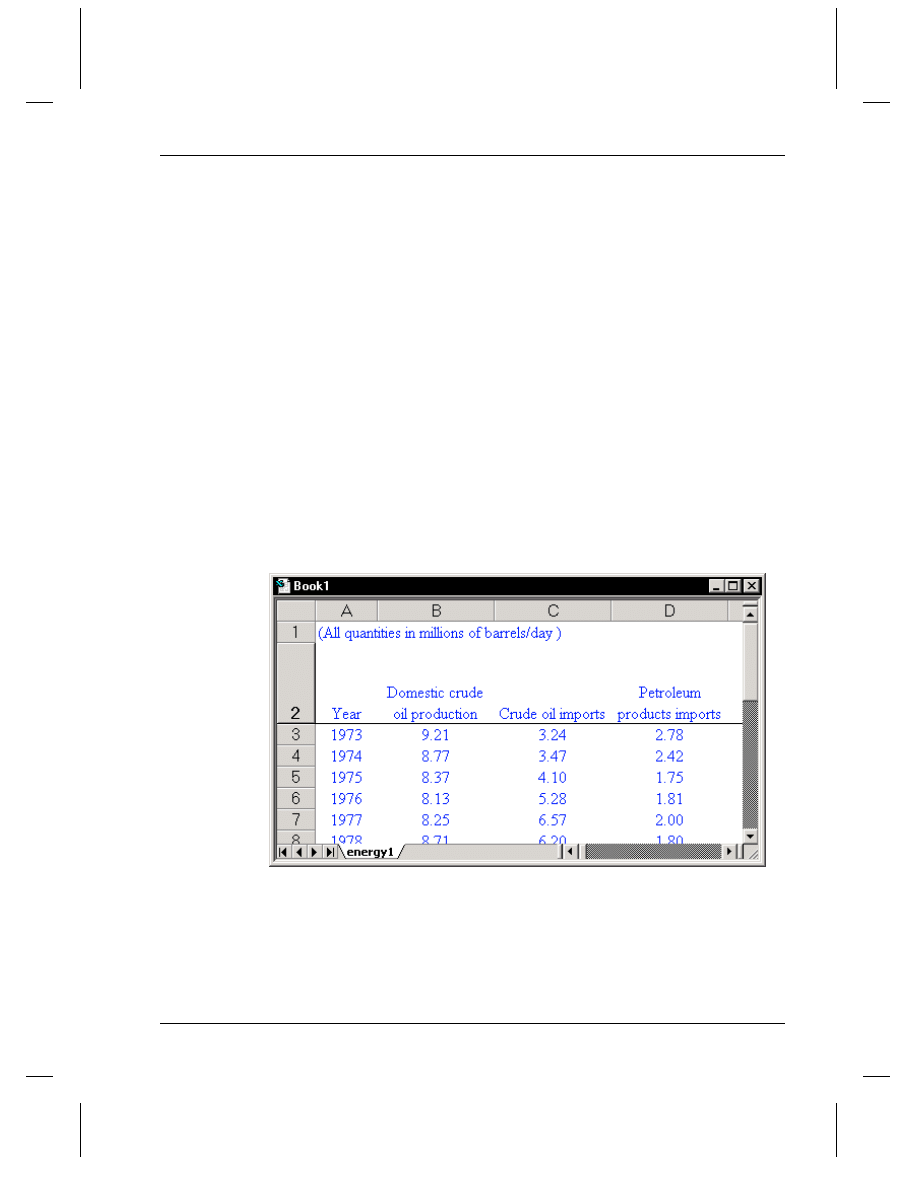
Chapter 4, Getting Started Using Origin

The Origin Workspace

•

The Layout menu is only available when a layout page is active. This
menu provides commands to:
=> add pictures of graphs or worksheets
=> view picture placeholders to increase redraw speed
=> view pictures using the screen driver to increase redraw speed
The Format menu provides layout page-specific commands to:
=> set the page display options

Excel Workbook Windows

You can open Excel workbooks inside Origin, combining Origin's
plotting and analysis power with Excel's spreadsheet tools. To plot your
workbook data in Origin, you must have Excel version 7 (Microsoft
Office 95) or later installed on your computer either as a local or network
copy.
Note: When you change the active window from an Excel workbook to
any other window type, the toolbar region displays a blank area where
the Excel toolbars were located. To hide this spacer, right-click in this
region and select Hide Toolbar Spacer from the shortcut menu.

Figure 29: Opening an Excel Workbook in Origin

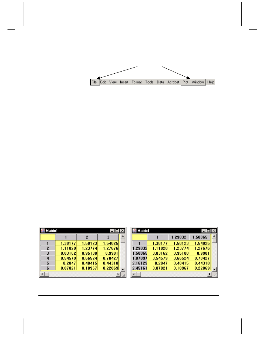
Chapter 4, Getting Started Using Origin

•

The Origin Workspace

Excel Workbook Menu Bar

Origin menus.

To open the Origin
Help file, right-click on
the workbook title bar
and select Help
Contents from the
shortcut menu.

When an Excel workbook is active in Origin, the menu bar displays both
Origin and Excel menus. The File, Plot, and Window menus are Origin
menus. All other menus are Excel menus.
The File menu provides Origin project and window commands.
The Plot menu provides commands to plot data into a specified graph
template.

The Window menu provides commands to:
=> set global preferences in the Options dialog box
=> control the display of the Project Explorer window, toolbars, and
Results Log
=> convert an Excel workbook to a matrix using direct conversion
=> arrange the windows in the workspace, open the Script window,
activate a Project Explorer folder, and activate a window in the
workspace

Matrix Windows

A matrix displays a single data set containing Z values. Instead of
displaying the data set as a column in a worksheet, a matrix displays the
data in a specified dimension of rows and columns. A matrix is linearly
mapped in X by columns and linearly mapped in Y by rows. By default,
the column and row numbers display in the column and row headings.
To display the X and Y values, select View:Show XY.

Figure 30: Showing the X and Y Matrix Values

Chapter 4, Getting Started Using Origin

The Origin Workspace

•

Origin provides a number of methods for converting a worksheet to a
matrix. This includes direct conversion, 2D binning, converting regular
XYZ data, and converting random XYZ data using gridding. These
conversion methods are available from the worksheet's Edit:Convert to
Matrix submenu.
When a matrix is active, you can create 3D, surface, contour, and image
plots.

Matrix Menu Bar

(See the Worksheet Menu Bar for commands that are available for all
window types.)
The File menu provides matrix-specific commands to:
=> import and export data
=> import and export image files
The Edit menu provides matrix-specific commands to:
=> convert the matrix to a worksheet
The View menu provides matrix-specific commands to:
=> when viewing an image, zoom in and out of the image
=> when viewing data, go to a specified row
=> switch between data mode and image mode
=> show the column and row numbers or show the XY mapping for the
Z values
The Plot menu provides commands to plot data into a specified graph
template.
The Matrix menu is only available when a matrix is active. This menu
provides commands to:
=> set matrix properties such as the internal data type and the display
format
=> set the matrix dimensions and the XY mapping relationship
=> use functions to set the matrix values or mathematically transform
values
=> transpose, invert, shrink using averaging, expand using bilinear
interpolation, smooth, or integrate the matrix
The Image menu is only available when a matrix is active. This menu
provides commands to:
=> display images using selected color palettes
=> open a tool to adjust the brightness and contrast in the image
The Tools menu provides matrix-specific commands to:
=> display the Tools toolbar tools in the "region of interest mode" for
selecting a region to copy, crop, or create a new matrix

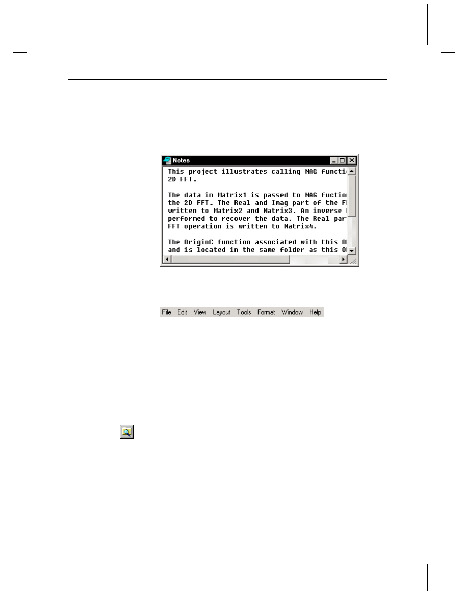
Chapter 4, Getting Started Using Origin

•

The Origin Workspace

Notes Windows

Notes windows can contain only text, and are thus used for recording
information.

Figure 31: A Notes Window

Notes Menu Bar

(See the Worksheet Menu Bar for commands that are available for all
window types.)
The View menu provides notes-specific commands to:
=> enable word wrapping

Project Explorer

Project Explorer is
shown or hidden by
clicking the Project

Explorer button

the Standard toolbar.

Project Explorer is a tool to help you organize your Origin projects. It is
particularly useful if you are working with a project that contains more
than a few windows. You can use Project Explorer to develop a folder
structure for organizing the windows in your project. You can also use
Project Explorer to control the view of your workspace.

When you first start Origin, Project Explorer displays docked to the
bottom edge of the workspace. You can dock it to any other edge or
display it as a window in the workspace. To prevent Project Explorer
from docking when positioning it as a window, press CTRL while
dragging.

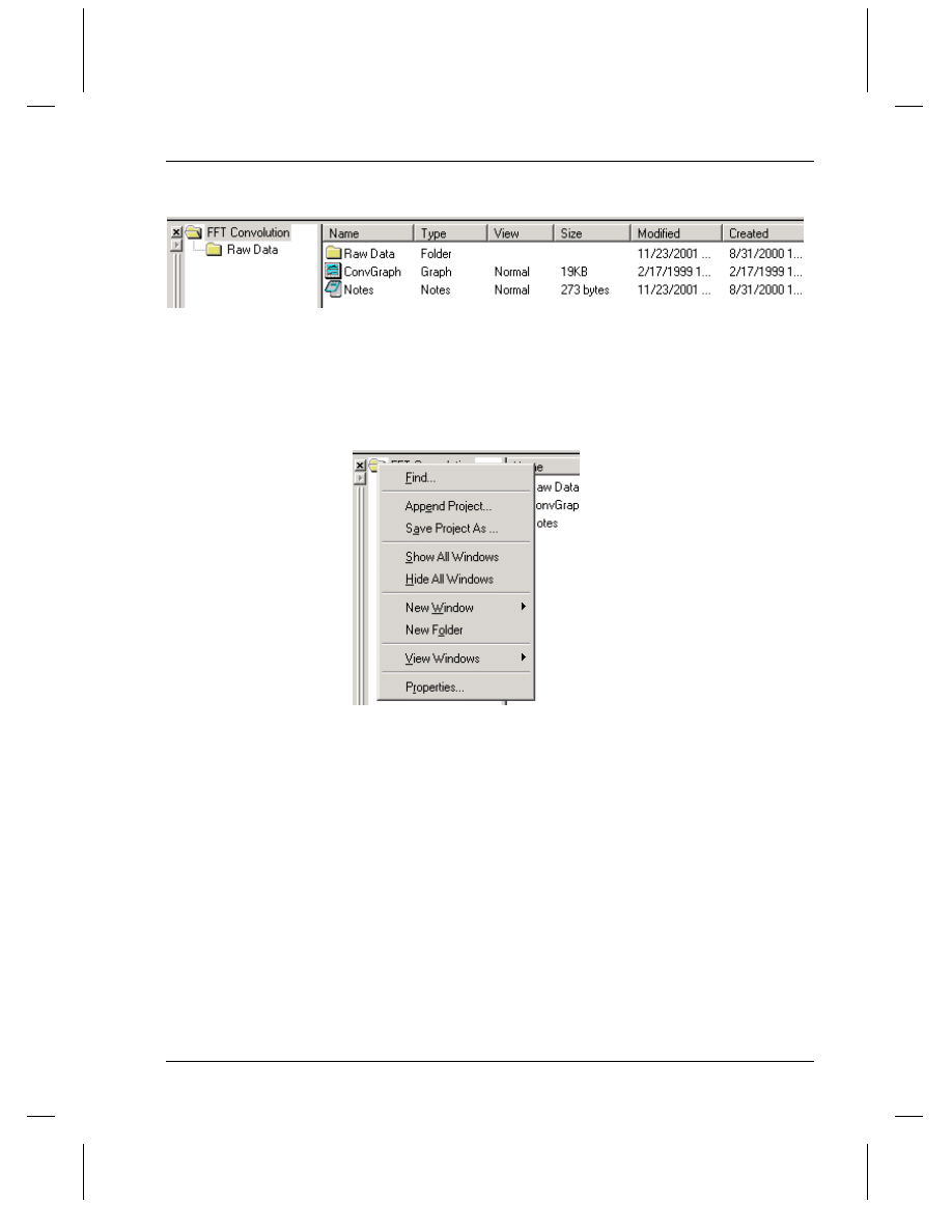
Chapter 4, Getting Started Using Origin

The Origin Workspace

•

Figure 32: Project Explorer

To create a new folder, right-click on the project folder (or a subfolder)
and select New Folder from the shortcut menu. Once you have created
one or more subfolders, you can move windows between folders.

Figure 33: Creating a New Folder

In addition to adding and moving folders, Project Explorer also controls
the view of your workspace. By default, only the windows in the active
Project Explorer folder display in your workspace. For projects with lots
of windows, this allows you to focus on specific windows in a clutter-
free workspace.
To control the view of the windows in your workspace, right-click on a
Project Explorer folder or right-click in a blank space on the left side of
Project Explorer. Select View:View Mode to alter the view mode.
(Alternatively, select View:View Windows:View Mode from the Origin
menu bar.)

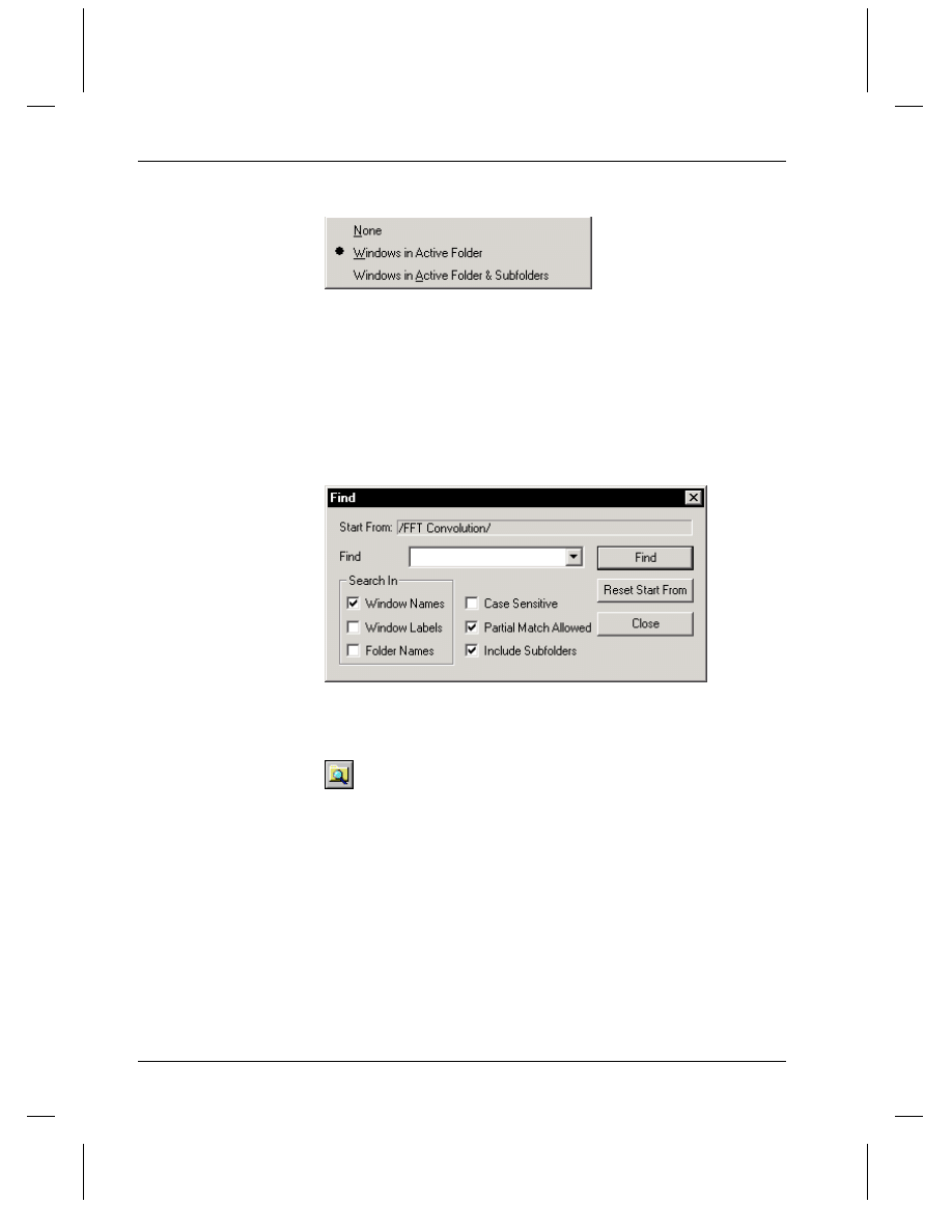
Chapter 4, Getting Started Using Origin

•

The Origin Workspace

Figure 34: Controlling the View of Windows in the Workspace

After you organize your windows into multiple folders, Project
Explorer's Find dialog box helps you locate windows in your project. To
open this dialog box, right-click on the Project Explorer folder that you
want to start your search from and select Find from the shortcut menu.
If you are unsure of the window location within your Project Explorer
folder structure, right-click on the main project folder and select Find.

Figure 35: Finding Windows in Your Project

Because Project Explorer uses some of your workspace, you may want to
close Project Explorer, even if you have already created a folder
structure. To close Project Explorer, click the Project Explorer button

on the Standard toolbar.

When Project Explorer is closed, Origin continues to use your folder
structure and view settings to display the windows in your workspace.
Thus, if you are working with a project that contains subfolders, and the
view mode is set to view only the active folder's windows, then Origin
will display the windows in your currently active folder.
To access windows in other folders, you can re-open Project Explorer or
you can select Window:Folders:Folder Name to view the windows in
the selected Project Explorer folder. The window list at the bottom of the
Window menu updates to reflect the windows in the Folder Name
folder.

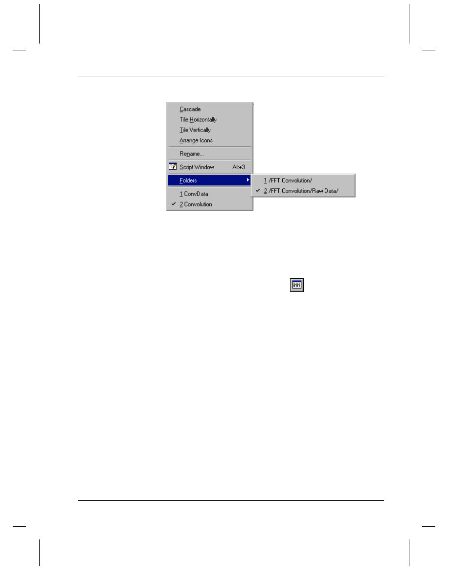
Chapter 4, Getting Started Using Origin

The Origin Workspace

•

Figure 36: Accessing Folders and Windows from the Menu Bar

Results Log

When you save an
Origin project, the
contents of the Results
Log is saved with the
project.

Origin automatically routes most analysis and fitting results to the
Results Log. In most cases, when results are output to the Results Log,
it opens automatically. However, to manually open (and close) the

Results Log, click the Results Log button

on the Standard toolbar.

Opening and closing the Results Log only controls its view state. You
do not lose results by closing the log.

When the Results Log first opens, it displays docked to the top edge of
the workspace. You can dock it to any other edge or display it as a
window in the workspace. To prevent the Results Log from docking
when positioning it as a window, press CTRL while dragging.
Each entry in the Results Log includes a date/time stamp, the window
name, a numeric stamp which is the Julian day, the type of analysis
performed, and the results.

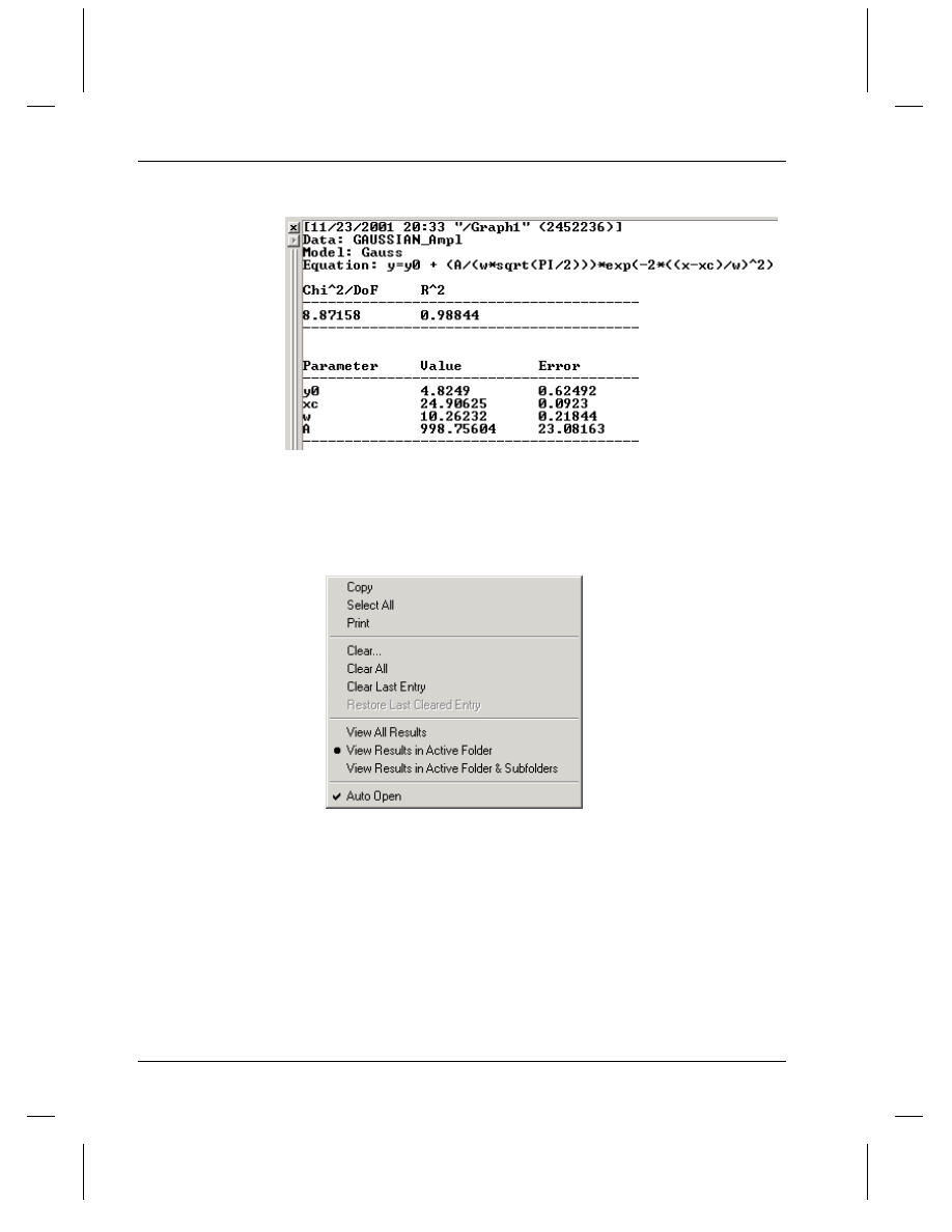
Chapter 4, Getting Started Using Origin

•

The Origin Workspace

Figure 37: The Results Log

You can right-click in the Results Log to open a shortcut menu with
commands to copy, print, clear, and view additional results.

Figure 38: The Results Log Shortcut Menu

Note: When you close the Results Log after it has been docked to the
edge of the workspace, the toolbar region may display a blank area where
the log was located. To hide this spacer, right-click in this region and
select Hide Toolbar Spacer from the shortcut menu.

Code Builder

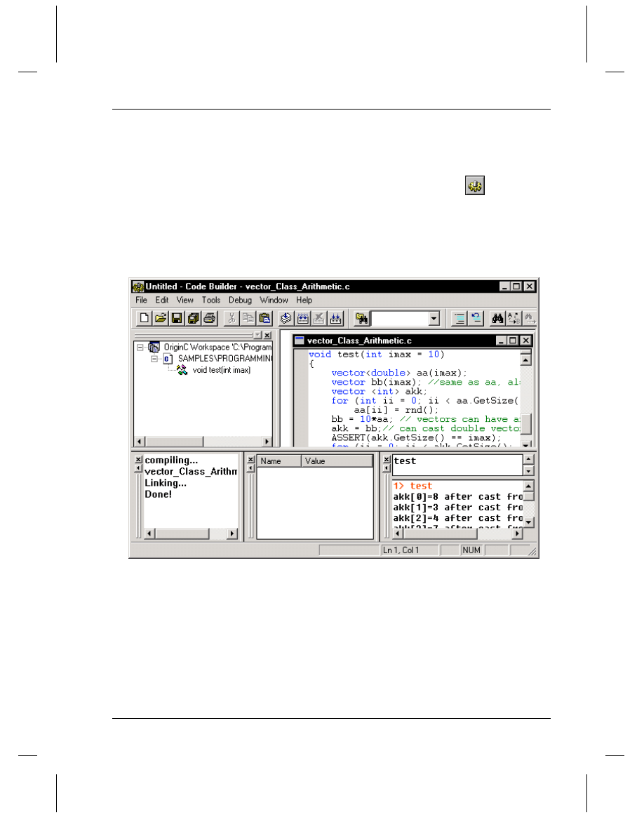
Chapter 4, Getting Started Using Origin

The Origin Workspace

•

Origin C is "Origin aware". This means that Origin objects such as
worksheets and graphs are mapped to classes in Origin C, allowing direct
manipulation of these objects and their properties from Origin C.
Origin C's integrated development environment is called Code Builder.

To open Code Builder, click the Code Builder button

on the

Standard toolbar. Code Builder provides tools for writing, compiling,
and debugging your Origin C functions. Once an Origin C function is
compiled, the function becomes accessible from Origin.

Figure 39: Code Builder

To learn more about programming in Origin, select
Help:Programming:Program Guide or review the sample Origin
projects located in the \Samples\Programming folder.

Script Window

The Script Window is available for executing LabTalk commands.
LabTalk is Origin's "historic" programming language. It has been
available in versions up to and including Origin 7. However, Origin 7

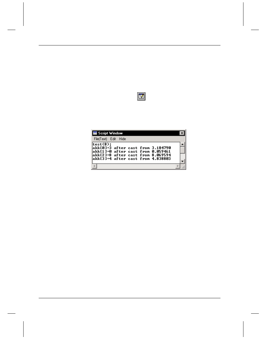
Chapter 4, Getting Started Using Origin

•

Origin Project Files

introduced the new Origin C programming language. Whereas LabTalk
scripts are interpreted during execution by Origin, Origin C code is
compiled to byte code form and therefore executes much faster than
LabTalk.
Even though Origin C is the preferred programming language in Origin
7, Origin C functions must be called using LabTalk commands. These
commands can be executed from the Script window, or from many other
locations that support LabTalk script. To open the Script window, click

the Script Window button

on the Standard toolbar. Note that when

you save an Origin project, the Script window contents are not saved
with the project.

Figure 40: The Script Window

To learn more about programming in Origin, select
Help:Programming:Program Guide or review the sample Origin
projects located in the \Samples\Programming folder.

Origin Project Files

Origin provides sample
project files in the
\Samples subfolders.

An Origin project file contains all the worksheet, matrix, graph, layout
page, and notes windows that are open in the workspace when you save
the project. These windows include minimized and hidden windows, as
well as windows that are accessible from other Project Explorer folders
in the current workspace.

Excel workbook windows are a special case. If a workbook is open in
the workspace, the project can be saved with a link to the source
workbook file, or the workbook can be saved internal to the project.
=> Saving the project with a link to the source workbook file allows you
to maintain an external Excel file that is updated when changes are made
to the associated workbook in Origin. This source file is also available
for use in other applications and can be accessed by other users.
=> Saving the workbook internal to the project enhances the project's
portability. You can open the project on any computer that has Origin

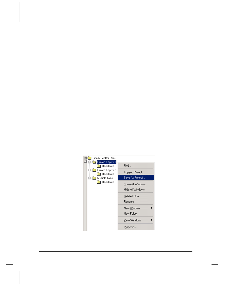
Chapter 4, Getting Started Using Origin

Origin Project Files

•

and Excel installed and have full access to your workbook data.
To control how the workbook is saved with the project, right-click on the
workbook window title bar and select Properties from the shortcut
menu.
In addition to these window types, the contents of the Results Log is
saved with an Origin project, as well as the current Project Explorer
folder and window structure.

Saving a Project

For information on
customizing the default
save path, see
"Opening an Existing
Project" on page 73.

To save a project to the current file name, select File:Save Project. If
the project has not been previously saved, this menu command opens the
Save As dialog box displaying the default file name, UNTITLED.OPJ,
in the File Name text box. Type the desired file name in the text box
(specify the path) and click Save to save the project.

To save the project to a new file name, select File:Save Project As. This
menu command also opens the Save As dialog box.
If you have developed a folder structure in Project Explorer, you can save
a selected folder and its subfolders to a new project file. To do this,
right-click on the Project Explorer folder that you want to save to a
project file and select Save As Project from the shortcut menu.

Figure 41: Saving a Project Explorer Folder to an Origin Project File

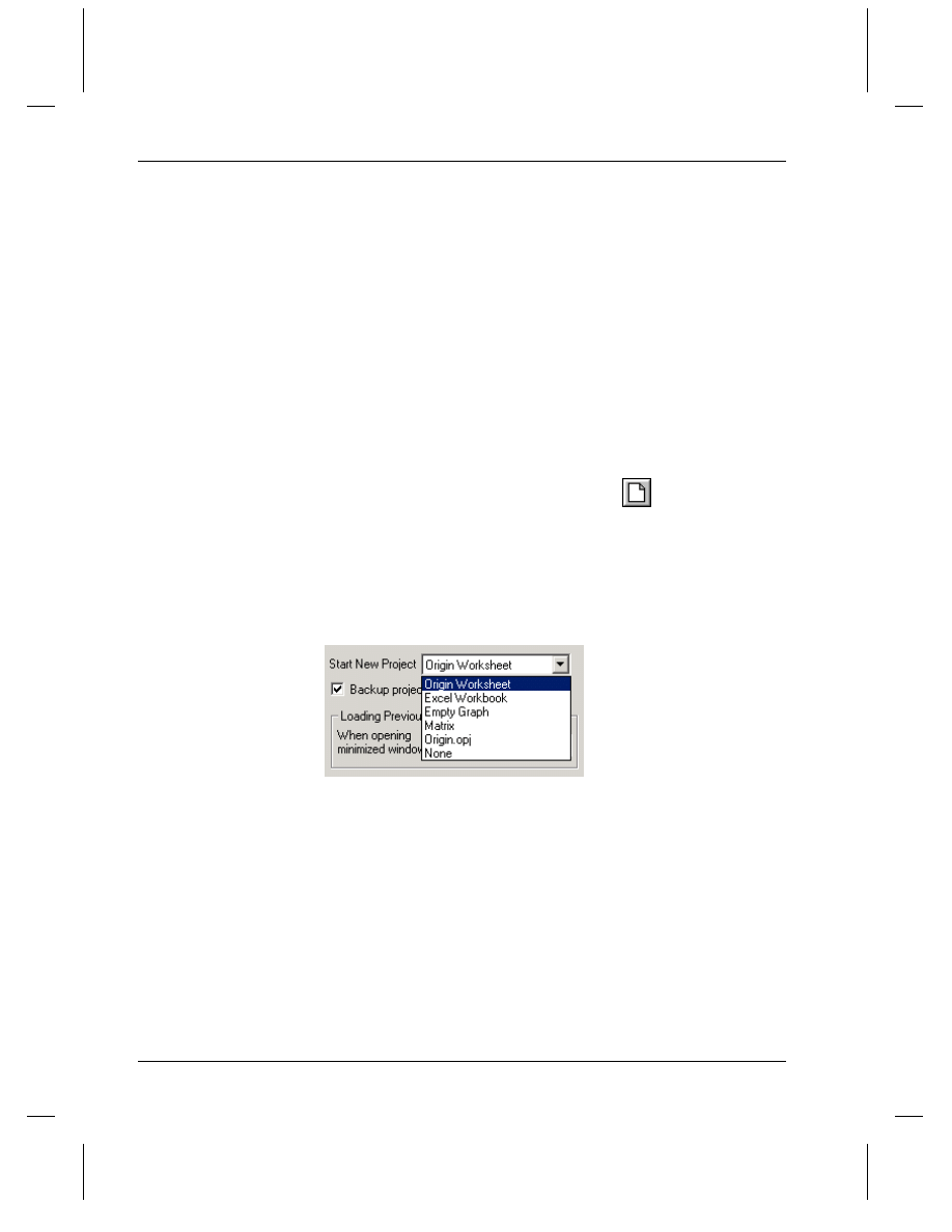
Chapter 4, Getting Started Using Origin

•

Origin Project Files

In this example, the Linked Layers 1 folder and its Raw Data subfolder,
all the windows that they contain, plus Results Log output specific to
these windows are saved to a new project file.

Automatically Creating a Backup

Origin will automatically create a backup of the currently saved project
file before re-saving. Origin renames the saved file BACKUP.OPJ, and
then saves the altered file using the specified file name.
The automatic backup feature is set on the Open/Close tab of the Options
dialog box (Tools:Options).

Opening a New Project

A new project is opened each time you start Origin. You can also open a

new project by clicking the New Project button

on the Standard

toolbar. In both cases, the new project contains one worksheet window.
You can, however, customize the new project that opens. To do this,
select Tools:Options to open the Options dialog box. Select the
Open/Close tab and then modify the Start New Project setting.

Figure 42: Customizing the New Project Setting

You can select from worksheet, Excel workbook, empty graph, matrix,
ORIGIN.OPJ, or none. The ORIGIN.OPJ file includes a worksheet and
a graph window. The graph window is configured to display a data plot
of column A (X values) and column B (Y values) automatically, after
you import or enter data into the worksheet columns. You can customize
the ORIGIN.OPJ project file and resave it. After you click OK in the
Options dialog box, you are asked if you want to save this setting for
future Origin sessions.

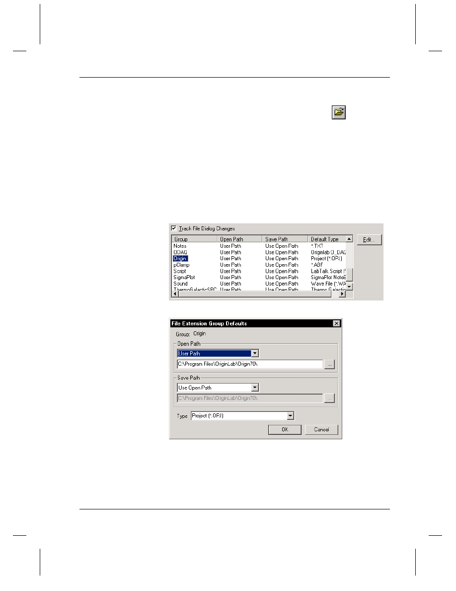
Chapter 4, Getting Started Using Origin

Origin Project Files

•

Opening an Existing Project

To open an existing project file, click the Open button

on the

Standard toolbar and select the desired file from the Open dialog box.
By default, Origin will keep track of the project file path, so that each
time you open a project in the current Origin session, the path to the last
opened file will be selected by default in the Open dialog box. To turn
off file tracking or to specify a custom project file path, select
Tools:Options to open the Options dialog box. Select the File Locations
tab. Select Origin from the top list box and then click Edit. This opens
the File Extension Group Defaults dialog box.

Figure 43: Customizing File Tracking

=> To specify a custom project file path, select User Path in the Open
Path group and then browse to the desired folder from the associated text
box. Click OK.
=> To set your Origin folder as the project file path, select Origin Path
from the Open Path drop-down list. Click OK.

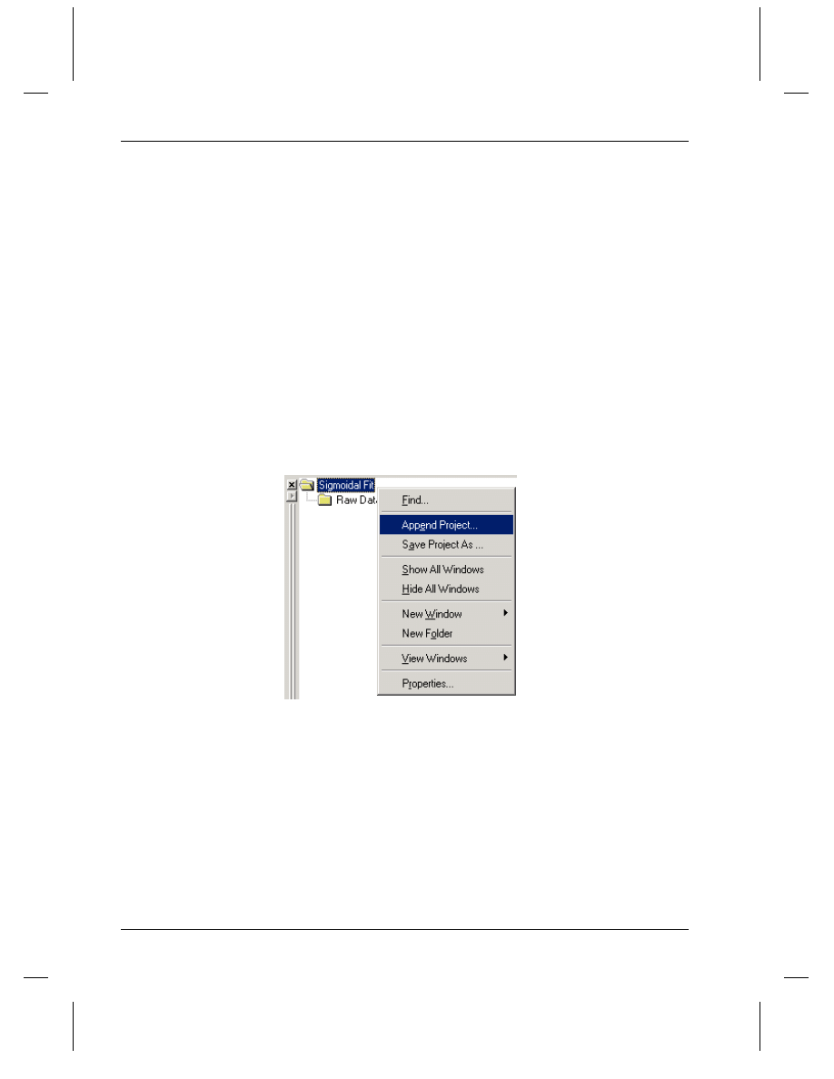
Chapter 4, Getting Started Using Origin

•

Origin Project Files

To direct Origin to always use this custom path, clear the Track File
Dialog Changes on the File Locations tab. Click OK. An Attention
dialog box asks if you want to save this setting for future Origin sessions.
Click Yes.

Opening More than One Project

Origin can only open one project at a time. To open multiple projects,
you must start multiple instances of Origin.

Appending Projects

The contents of a project can be added to the currently opened project by
selecting File:Append or by right-clicking on a Project Explorer folder
and selecting Append Project from the shortcut menu.

Figure 44: Appending Projects

To re-activate the
display of Reminder
Message boxes, select
Tools:Reactivate
Reminder Messages.

After you select the project to append, Origin displays a Reminder
Message asking if you want to append the contents of the new project
into a new Project Explorer folder or into the current folder.
If duplicate window names exist between projects, Origin automatically
changes the name of the appended window by adding an "A" to the
window name (AWindowName). For example, in the following figure, a
project containing a Data1 worksheet is appended to a project that also
contains a Data1 worksheet. The appended window is renamed AData1.

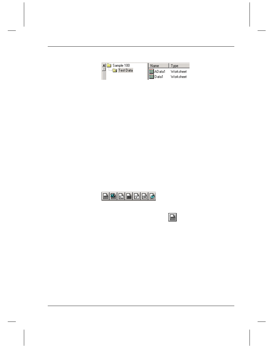
Chapter 4, Getting Started Using Origin

Project Windows

•

Figure 45: Renaming Duplicate Window Names when Appending

Project Windows

To learn how to
organize your project
using Project Explorer,
see "Project Explorer"
on page 64.

Project windows include worksheet, matrix, Excel workbook, graph,
layout page, and notes windows. You can create and open any number
of windows in an Origin project. The only limitation is your machine's
memory. However, you should keep your projects manageable by
limiting the number of windows contained in a project. You should also
consider organizing the windows using Project Explorer.

Creating a New Window

To create a new window, click one of the New Window buttons on the
Standard toolbar.

Figure 46: New Window Buttons on the Standard Toolbar

To learn more about
templates, see
"Window Templates"
on page 80.

These buttons create windows based on a default template. For

example, the New Worksheet button

creates a worksheet based on

the ORIGIN.OTW template. You can change the template that is
associated with any of these buttons. To do this, select File:New to
open the New dialog box. To change the template associated with the
New Worksheet button, select Worksheet from the list box, then select
the desired template from the Template group. Click Set Default to
associate this template with the New Worksheet button.

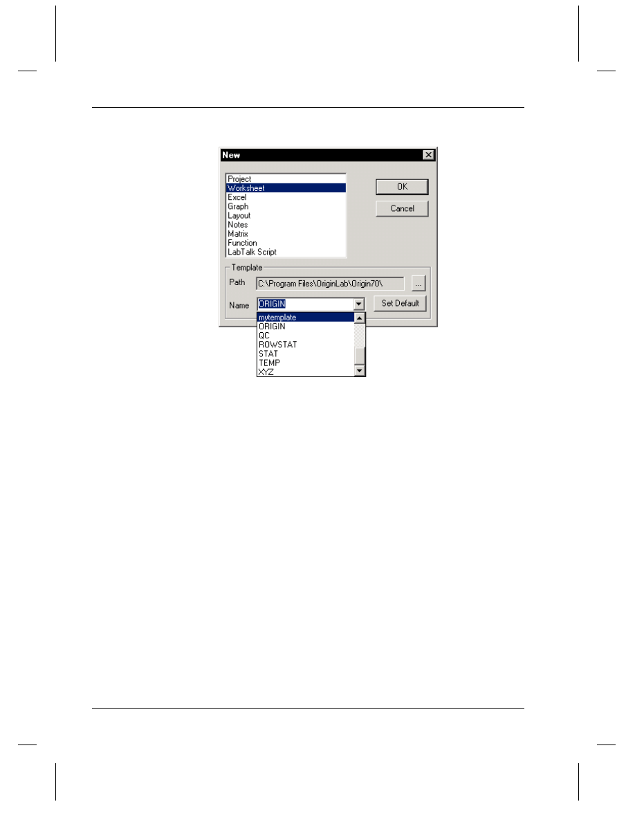
Chapter 4, Getting Started Using Origin

•

Project Windows

Figure 47: Changing the Template for the New Worksheet Button

You can also use the New dialog box to create new windows based on
specific templates.

Renaming a Window

To rename a worksheet, matrix, graph, layout page, or notes window,
activate the window and then select Window:Rename. Alternatively,
right-click on the window's title bar and select Rename from the shortcut
menu. Both menu commands open the Rename dialog box.
To rename an Excel workbook window, right-click on the window's title
bar and select Properties from the shortcut menu.
When renaming windows, consider the following:
=> The window name cannot start with a numeral.
=> Origin ignores any spaces between characters.
=> The name cannot exceed 13 characters in length.
For greater flexibility in window naming, include the Label field in the
window title bar. The label allows more characters and accepts special
characters (for example, an underscore and dollar sign). It also allows
spaces between characters.

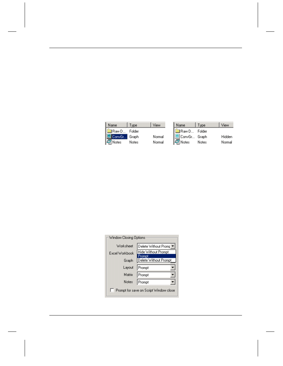
Chapter 4, Getting Started Using Origin

Project Windows

•

Hiding a Window

To maximize the use of your workspace, you can hide windows from
view - without deleting them from the project. To hide a window in the
workspace, select the desired window icon on the right side of Project
Explorer and then double-click on this icon. To return the window to the
normal view mode, double-click again on the window icon. These view
controls are also available by right-clicking on the window icon in
Project Explorer, or by right-clicking on the window title bar.

Figure 48: Hiding a Window from View

Deleting a Window

When you delete a
window, it is no longer
a part of the project.

To delete a window from the project, click the X button in the upper-
right corner of the window. Origin then asks you if you want to hide or
delete the window.

To prevent this verification prompt from displaying, select
Tools:Options to open the Options dialog box. Then select the
Open/Close tab. In the Window Closing Options group, select how you
want Origin to respond when you click a particular window type's close
button.

Figure 49: Setting the Close Option for a Window Type

Chapter 4, Getting Started Using Origin

•

Project Windows

Refreshing a Window

Whenever you change the contents of a graph window or a worksheet, or
expose a part of a window that was hidden, Origin automatically redraws
the affected portion of the window. Occasionally, a portion of the
window may not refresh correctly. Whenever this occurs, click the

Refresh button

on the Standard toolbar to refresh the active window.

Note: To control the percentage of the window that must be exposed
before Origin automatically redraws the window, select Tools:Options
to open the Options dialog box. Select the Miscellaneous tab and then
edit the No Redraw (% Covered) combination box.

Duplicating a Window

To duplicate the active worksheet, graph, matrix, or layout page window,

click the Duplicate button

on the Standard toolbar. When a

duplicate window is created, Origin names the window using the default
window name syntax:
DefaultWindowNameN
where N is assigned the lowest available number not used by other
window names (of the same type) in the project.

Table 1: Default Window Names

Window

Default Name

Worksheet

WorksheetN

Graph

GraphN

Matrix

MatrixN

Layout Page

LayoutN

Function Graph

FunctionN

Saving a Window

In addition to saving projects, windows (except for layout pages) can be
saved to a file. When a window is saved to a file, the window can be
opened in any other Origin project. To save the active window to a file,
select File:Save Window As. This menu command opens the Save As
dialog box. Origin automatically lists the correct file extension for the
active window type in the Save as Type drop-down list.

Chapter 4, Getting Started Using Origin

Project Windows

•

Table 2: Window File Extensions

Window

File Extension

worksheet

.OGW

matrix

.OGM

graph

.OGG

Excel workbook

.XLS

notes

.TXT

Opening a Window from a File

To learn how to
append projects, see
"Appending Projects"
on page 74.

If you have a window in one project that you want to include in another
project, you can append the projects. However, this action will add all
the windows from a selected project into the currently open project. To
"append" only the desired window, you must save the window to a file
and then open the window in the desired project. To open a worksheet,
graph, matrix, or notes window that was saved to a file, click the Open

button

on the Standard toolbar. This button opens the Open dialog

box. From the Files of Type drop-down list, select:

‘Worksheets (*.OGW)’ to open a worksheet window.
‘Graphs (*.OGG)’ to open a graph or function graph window.
‘Matrix (*.OGM)’ to open a matrix window.
‘Text (*.TXT)’ to open a notes window.
After you open a worksheet, graph, matrix, or notes window file in a
project and then save the project, the window then remains a part of this
project.

To open an Excel workbook file, click the Open Excel button

on the

Standard toolbar. After you select your Excel file, a dialog box opens
asking if you want to open the workbook as an Excel workbook or as an
Origin worksheet.

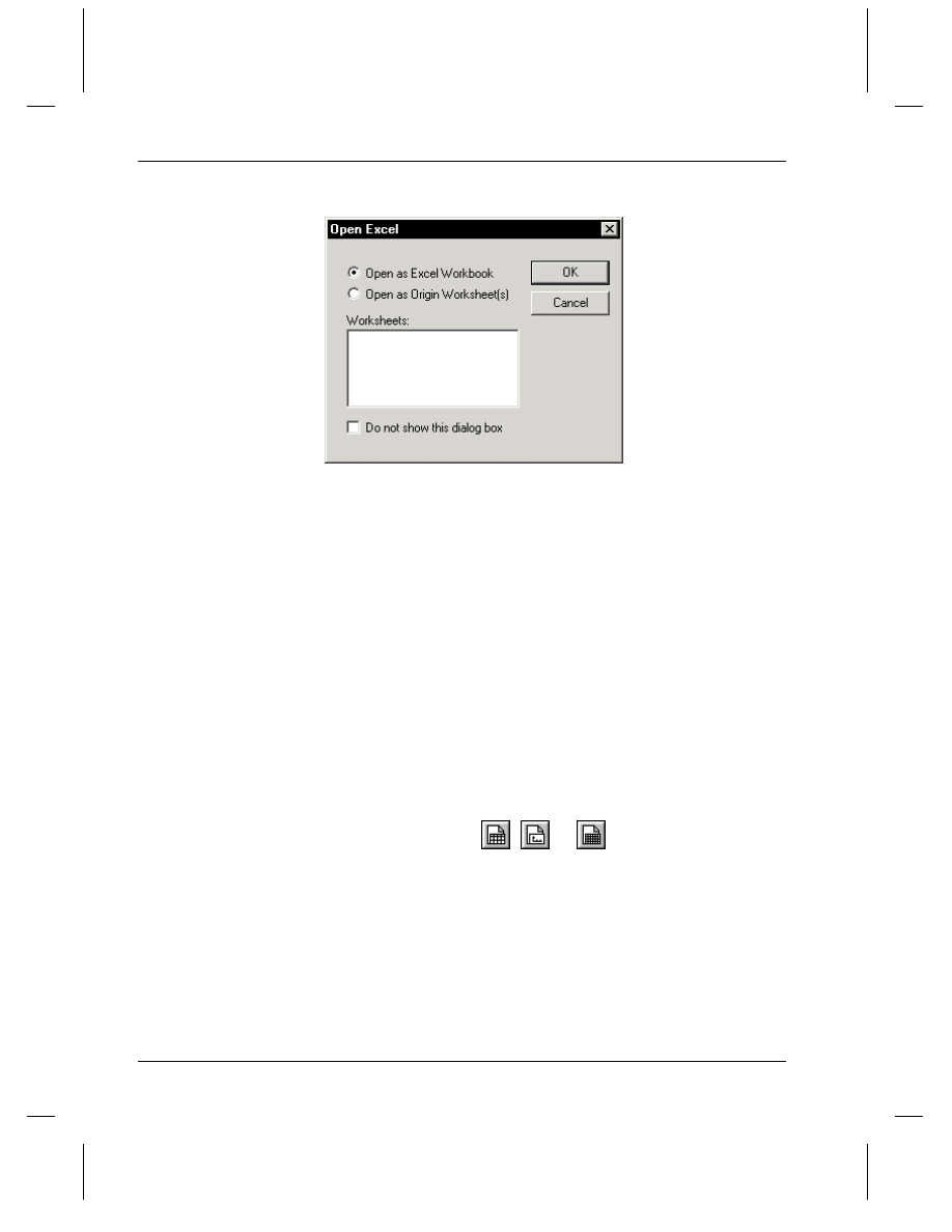
Chapter 4, Getting Started Using Origin

•

Window Templates

Figure 50: Opening an Excel Workbook

If you open the workbook as a workbook, you can continue to use Excel's
spreadsheet tools to process your data, all within the Origin workspace.
You also have access to Origin's plotting and analysis tools. When you
are ready to save your project, you can save the project with a link to
your source workbook, and update the link, or you can save the
workbook as part of your Origin project. When you update the link to a
(linked) workbook, the updated workbook is available for other
applications or other users.
If you open the workbook as one or more Origin worksheets, you have
no access to Excel's spreadsheet tools in Origin. Furthermore, the data
no longer has a connection to the source workbook. Thus, the changes
you make to the data are lost to the original workbook.

Window Templates

When you create a new worksheet, graph, or matrix window, (for

example, by clicking the

, or

button on the Standard

toolbar), Origin creates the new window based on a template. The
template determines the properties of the new window. For example, if
the new window is a worksheet, the template determines the number of
columns in the worksheet, each column's plotting designation and display
type, the ASCII import settings, and any formulas used to set the column
values. If the new window is a graph, the template determines the
number of layers (sets of XY axes) on the page and their arrangement,
the types of data plots in each layer (for example, scatter or bars), the
number of data plots, the axes scale type, and text labels and other
annotations. Basically the template determines all the attributes of the

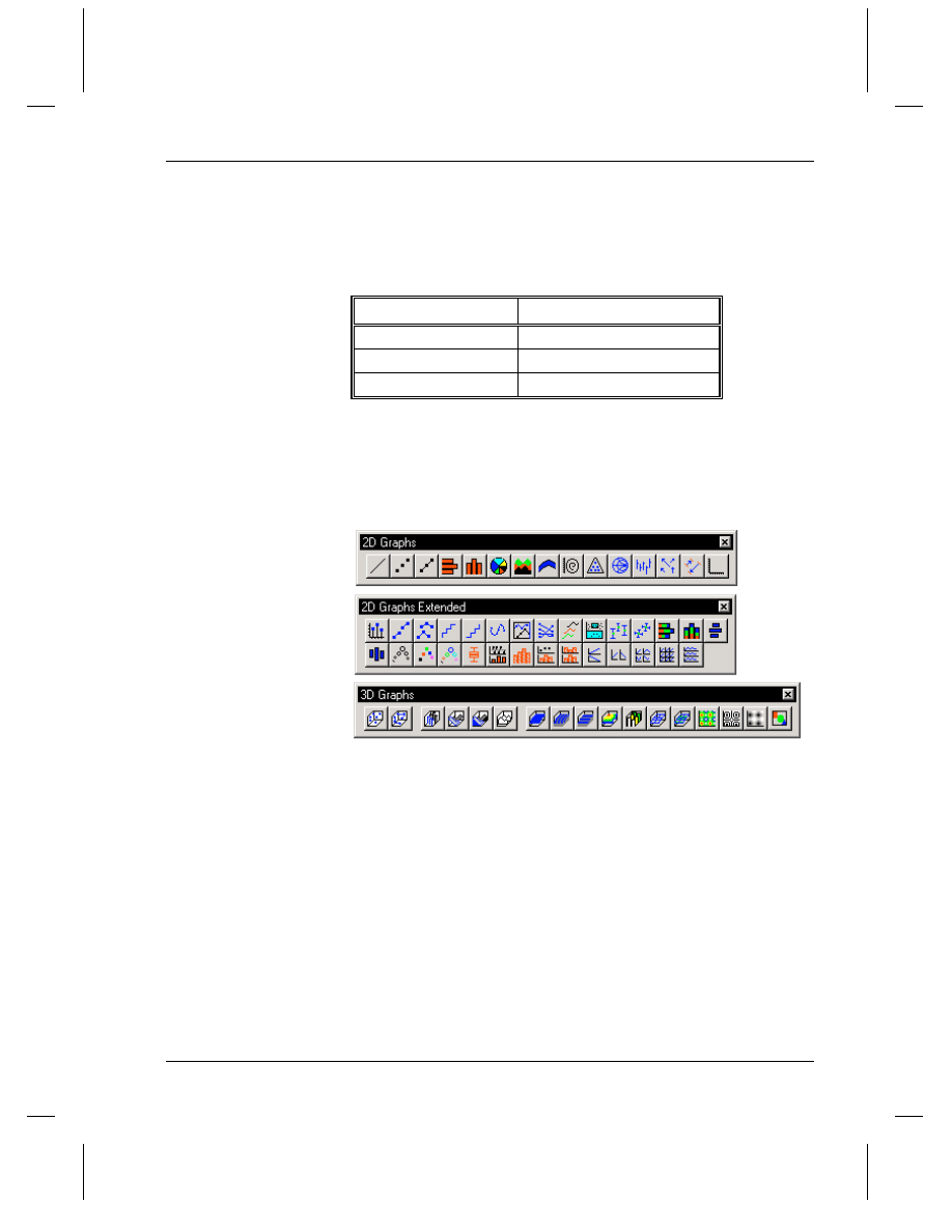
Chapter 4, Getting Started Using Origin

Window Templates

•

window, except for the actual data the window will contain. Data is
never saved with a template.
The following table lists the file extensions for the templates.

Table 3: Template File Extensions

Window

Template File Extension

worksheet

.OTW

graph or function graph

.OTP

matrix

.OTM

Origin provides many built-in templates. For example, most of the graph
templates are accessible from the plotting toolbar buttons.

Figure 51: Plotting Toolbar Buttons

Origin also provides a Template Library tool for categorizing and
accessing graph templates. To open the Template Library tool when a
worksheet or an Excel workbook is active, select Plot:Template
Library.

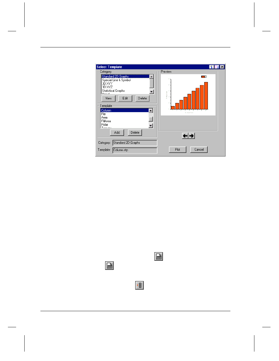
Chapter 4, Getting Started Using Origin

•

Window Templates

Figure 52: The Template Library Tool

You can also use the Template Library tool to plot your worksheet or
Excel workbook data. If you highlighted data in the worksheet or
workbook before opening the tool, and your data selection is appropriate
for the template you've selected, then click the Plot button to plot the data
into the template. If you did not highlight data or if your selection was
not appropriate for the template you've selected, then click the Plot
button to open an intermediary dialog box for data selection.

To create a custom template, you can modify an existing template or
create a new template. The procedure is similar in both cases. You must
first open a window based on a built-in template, customize the
properties of the objects in the window, and then save the window as a
template. The instructions on re-building the window are saved with the
template. However, any data in the window is not saved with the
template.
For example, suppose you want to customize the template associated

with the New Worksheet button

on the Standard toolbar. To do this,

click

to open a new worksheet. Now customize the attributes of this

worksheet. For example, perhaps you always import ASCII data files
that contain data in the format X, Y, Y Errors. In this case, click the Add

New Columns button

on the Standard toolbar. Then right-click on

the new column (C) and select Set As:Y Error from the shortcut menu.

Chapter 4, Getting Started Using Origin

Window Templates

•

To save this window as a template, select File:Save Template As. The
built-in template ORIGIN.OTW is listed by default in the File Name text
box. If you click Save, you will overwrite the built-in template with your
custom settings. Alternatively, you can type a new file name to save
your changes to a new template.
If you save to a new file name, you can associate the New Worksheet

button

with this new template file (it is currently linked to

ORIGIN.OTW). To do this, select File:New to open the New dialog
box. Select Worksheet from the list box. Then select your new template
file from the Template group. Finally, click the Set Default button to
associate this template with the New Worksheet button.

Chapter 4, Getting Started Using Origin

•

Window Templates

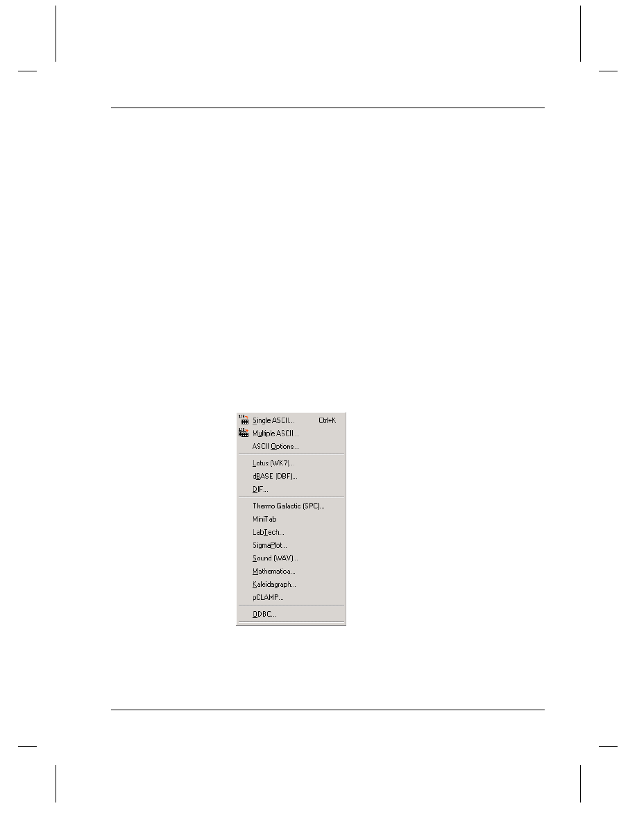
Tutorial 1, Plotting Your Data

Introduction

•

Tutorial 1, Plotting Your Data

Introduction

This tutorial will show you how to import ASCII data into a worksheet,
plot the data, and then customize some basic elements of the graph.

Importing Your Data

Origin imports data stored in a wide variety of formats. These import
options are available from the worksheet's File:Import submenu.

Figure 1: Importing Data into a Worksheet

When you import data from this submenu, Origin allows you to control
the default folder that is listed in the associated "Open" dialog box. To
do this, select Tools:Options to open the Options dialog box. Then

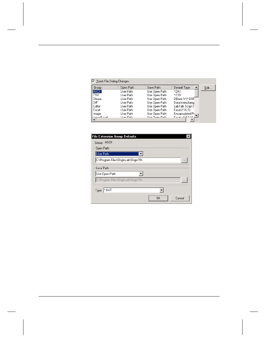
Tutorial 1, Plotting Your Data

•

Importing Your Data

select the File Locations tab. Select the desired data type from the top
list box and then click the Edit button.

Figure 2: Customizing the Default Folder for the Import Data Types

If your data files are stored in the same location as your Origin project
files, then select Project Path from the Open Path drop-down list. Click
OK in this dialog box and in the Options dialog box. To save the settings
for the next Origin session, click Yes at the Attention prompt.
In addition to the menu commands, you can also drag-and-drop ASCII,
SigmaPlot, Minitab, and Thermo Galactic SPC files into Origin. Once
you have selected the file in Windows Explorer, if Origin isn't currently
open you can drag the file onto your Origin desktop icon. If Origin is
already open, you can drag the file over the Origin taskbar button and
hold there until Origin becomes active. Then continue dragging and drop
the file into the Origin workspace.

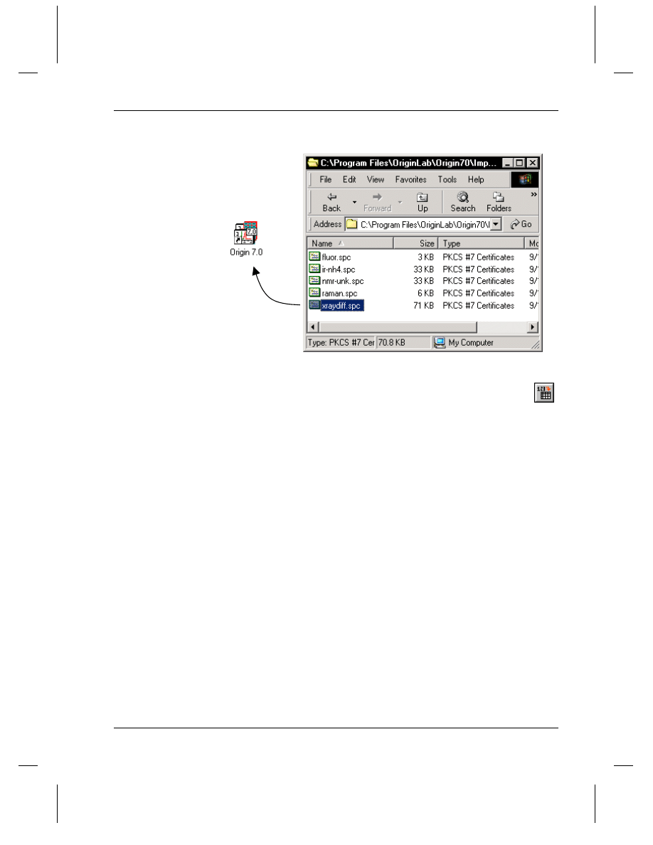
Tutorial 1, Plotting Your Data

Importing Your Data

•

Figure 3: Dragging a Data File Onto Your Origin Desktop Icon

Drag-and-drop the

file onto your

desktop icon.

If you customize the
ASCII Import Options
settings, you can save
your worksheet as a
template to access the
settings in the future.

When you import ASCII data by dropping into Origin, by selecting

File:Import:Single ASCII, or by clicking the Import ASCII button
on the Standard toolbar, Origin uses the import settings defined in the
ASCII Import Options dialog box. The default import settings will work
well with many ASCII files. However, with complex ASCII files, you
may need to customize these settings. To open the ASCII Import
Options dialog box, select File:Import:ASCII Options.

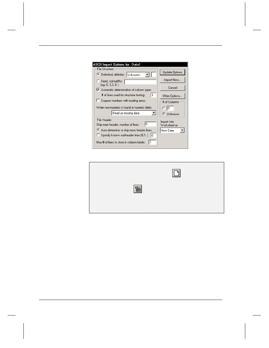
Tutorial 1, Plotting Your Data

•

Importing Your Data

Figure 4: Customizing the ASCII Import Settings

To Import the ASCII File:

1) Begin this lesson by clicking New Project

on the Standard

toolbar.

2) Click Import ASCII

on the Standard toolbar.

3) In the Origin \TUTORIAL folder, select TUTORIAL_1.DAT from
the list of files.
4) Click Open. The ASCII file imports into the worksheet.

The worksheet is renamed using the name of the ASCII file you
imported. Because the file contains text in the first two rows, the first
row of text is used to rename the columns, while the first and second
rows of text are used to create column labels. The labels are used for the
text in the legend when a graph is created.
Note: You may need to resize the worksheet to see all the columns.

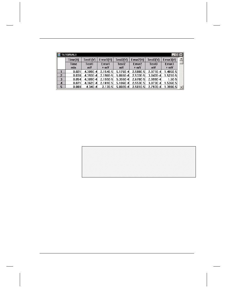
Tutorial 1, Plotting Your Data

Designating Worksheet Columns as Error Bars

•

Figure 5: Importing the ASCII File

Designating Worksheet Columns as Error Bars

When you import data into a worksheet, the default column designations
of X, Y, Y, Y, etc. are used to show data associations. If your data is
associated differently, you can manually set the column designations.
In this example, the data has the following associations: X, Y, Y Error,
Y, Y Error, Y, Y Error.

To Designate Columns as Error Bars:
1) Click on the Time(X) column heading and drag to the Error3(Y)
column heading.
2) Right-click within the highlighted cells to open a shortcut menu.
3) Select Set As:XYYErr from the shortcut menu. This changes the
Error1, Error2, and Error3 columns to error bar columns.

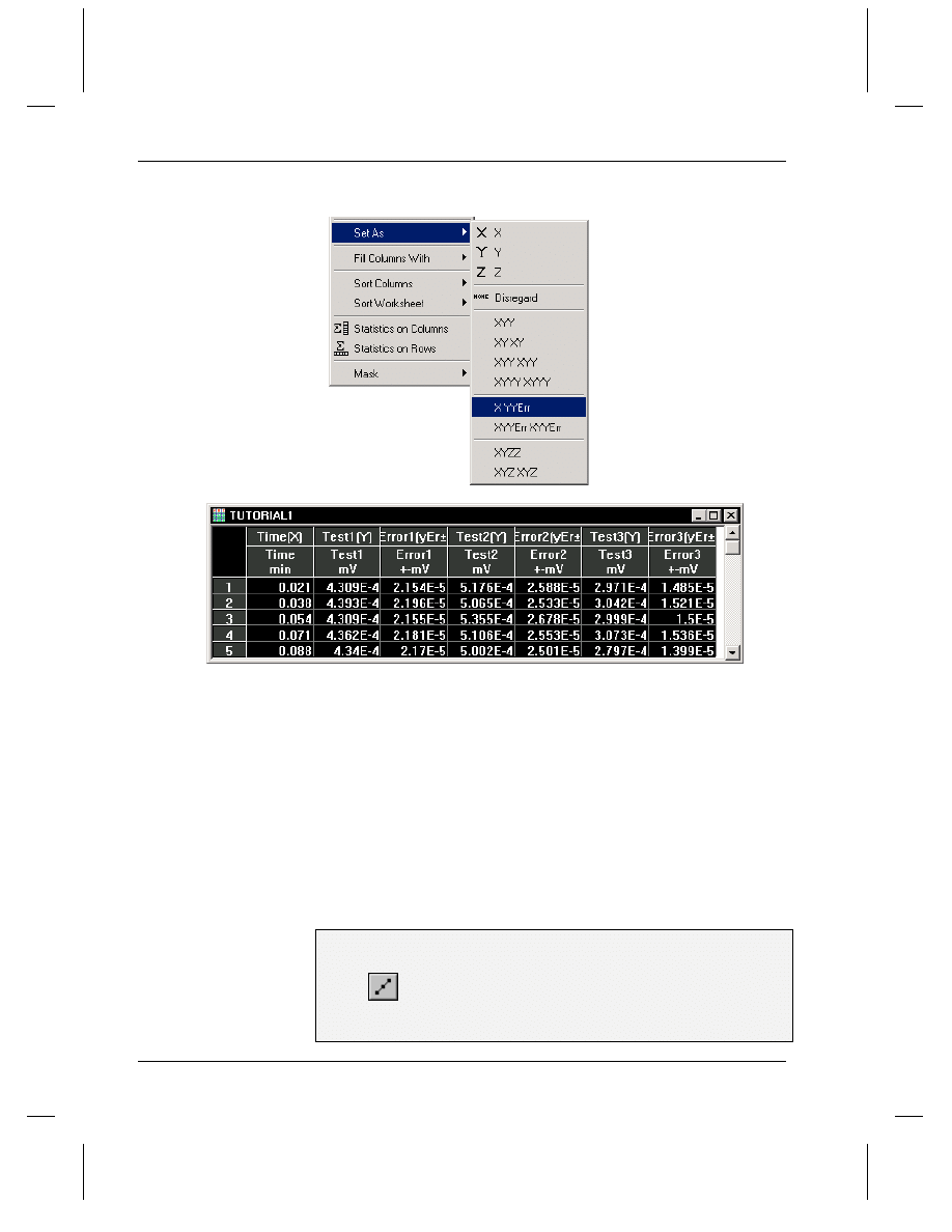
Tutorial 1, Plotting Your Data

•

Plotting Your Data

Figure 6: Setting the Column Designations

Plotting Your Data

Origin offers a broad range of plotting options. The quickest way to
create a graph is to select your worksheet data by highlighting the
column(s), and then clicking a button on one of the plotting toolbars.
When you plot multiple columns using this technique, Origin
automatically groups the data plots and increments attributes such as the
symbol type and color, so that you can easily distinguish between data
plots.

To Plot Your Worksheet Data:
1) With your worksheet data still selected, click the Line + Symbol

button

on the 2D Graphs toolbar. The three Y columns are plotted

as line and symbol data plots with error bars provided by the error bar
columns to the right of the associated Y columns.

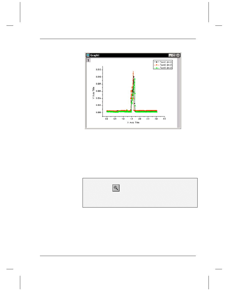
Tutorial 1, Plotting Your Data

Plotting Your Data

•

Figure 7: Plotting the Worksheet Data

Focusing on a Region of Your Graph

You may want to take a closer look at interesting areas of your data,
particularly if you have a large number of points. Origin provides a
number of tools to accomplish this, including the Enlarger tool. The
Enlarger tool automatically rescales the axes of the graph to show only
the region of the data plot(s) you select.

To Enlarge a Section of Your Data:

1) Click Enlarger

on the Tools toolbar.

2) Click-and-drag with the magnifying glass cursor to draw a box around
the large peaks (near X = 1.5) in the graph window. Release the mouse
button to complete the operation.

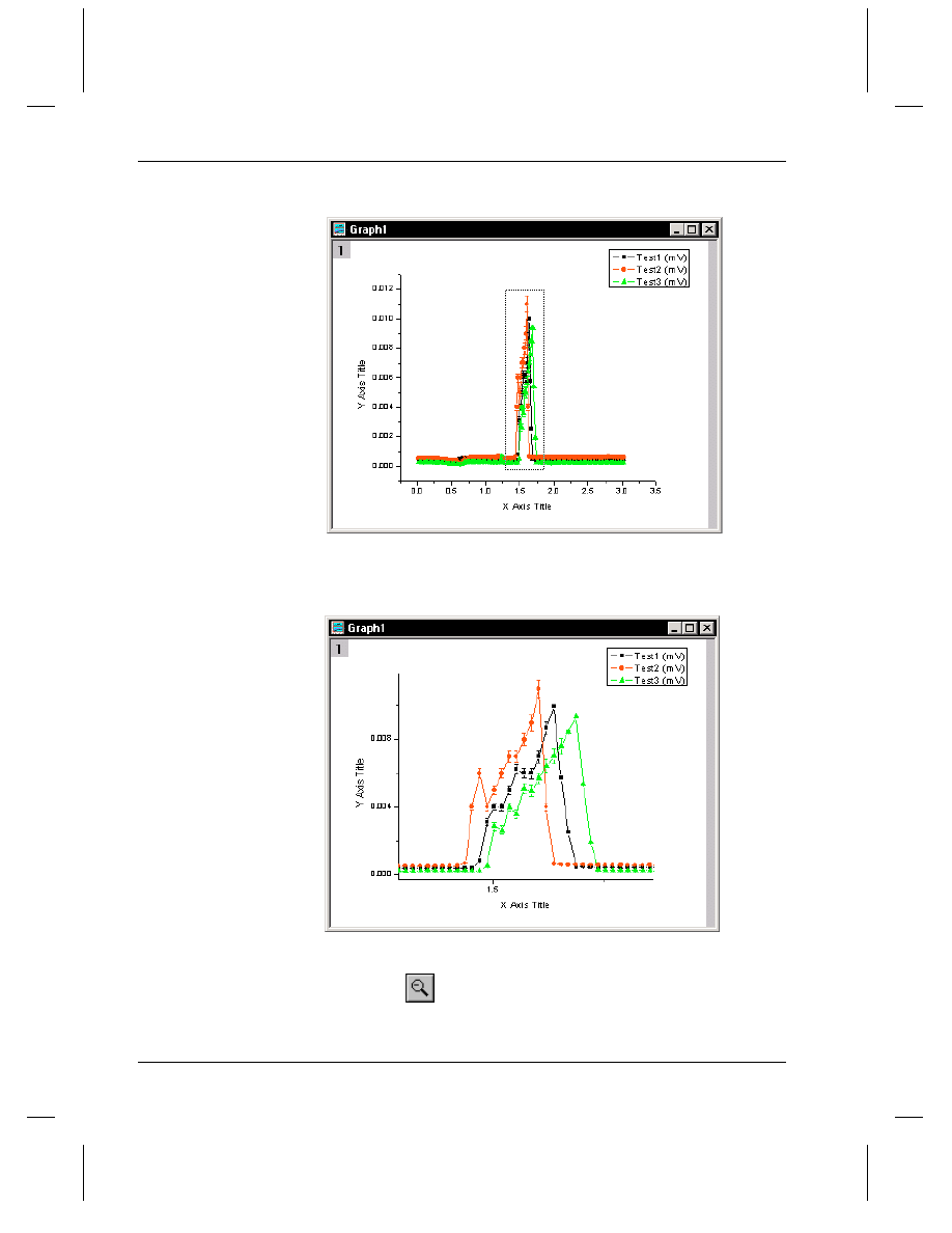
Tutorial 1, Plotting Your Data

•

Plotting Your Data

Figure 8: Enlarging a Section of Your Data

Figure 9: Rescaled Graph

Note: To return the axes to their original scale, click on the Undo

Enlarge tool

on the Tools toolbar.

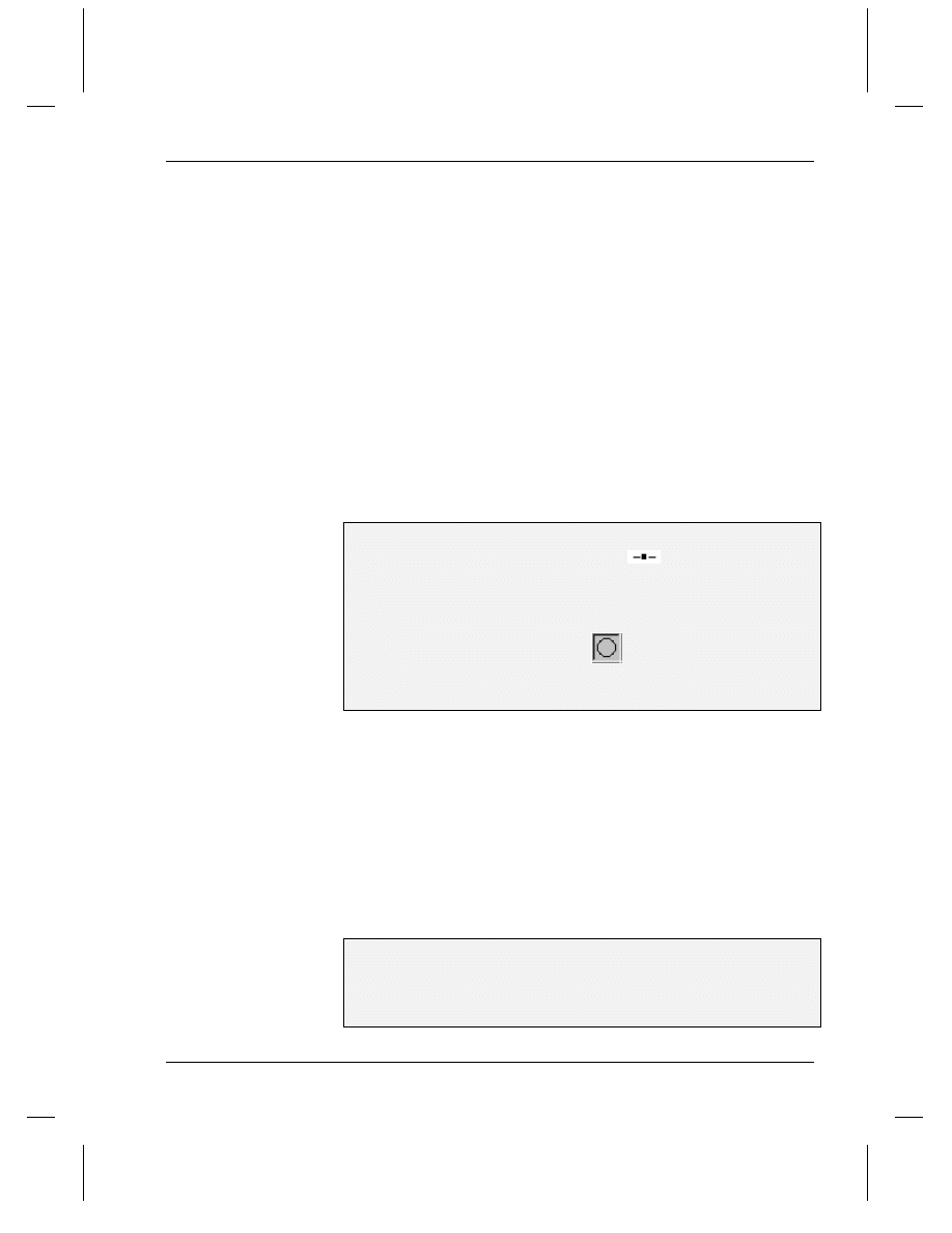
Tutorial 1, Plotting Your Data

Customizing the Graph

•

Customizing the Graph

Origin allows you to customize every aspect of your graph. The easiest
way to customize graphic elements is to double-click on them.

Customizing the Data Plot

Double-clicking on a data plot or the data plot icon in the legend opens
the Plot Details dialog box. This dialog box allows you to customize the
data plot you selected, as well as all the features of the graph window
except for the axes and text labels. The selection on the left side of the
dialog box determines the controls available for customizing on the right
side of the dialog box. For example, when a line and symbol data plot is
selected, you can edit the attributes of the lines and symbols, draw drop-
lines to either axis, and select which features are incremented between
the grouped data plots.

To Customize the Data Plot:
1) Double-click on the Test1 data plot icon

in the legend. The Plot

Details dialog box opens with the TUTORIAL1:Time(x), Test1(Y) data
plot icon selected on the left side of the dialog box.
2) Select the Symbol tab if it is not currently selected.

3) Select the open circle symbol type

from the Preview drop-down

list.
4) Click OK.

Note: Because the data plots are grouped, the symbol type of the Test2
and Test3 data plots change to increment from the open circle symbol
selected for the Test1 data plot.

Customizing the Axes

Double-clicking on any of the axes in the graph opens the Axis dialog
box. Similar to the Plot Details dialog box, you can specify the axis you
want to customize by selecting it from the Selection list box on the left
side of the dialog box.

To Customize the Axes:
1) Double-click on the X axis.
2) On the Scale tab, type 1.2 in the From text box, 1.8 in the To text box,
and .1 in the Increment text box.

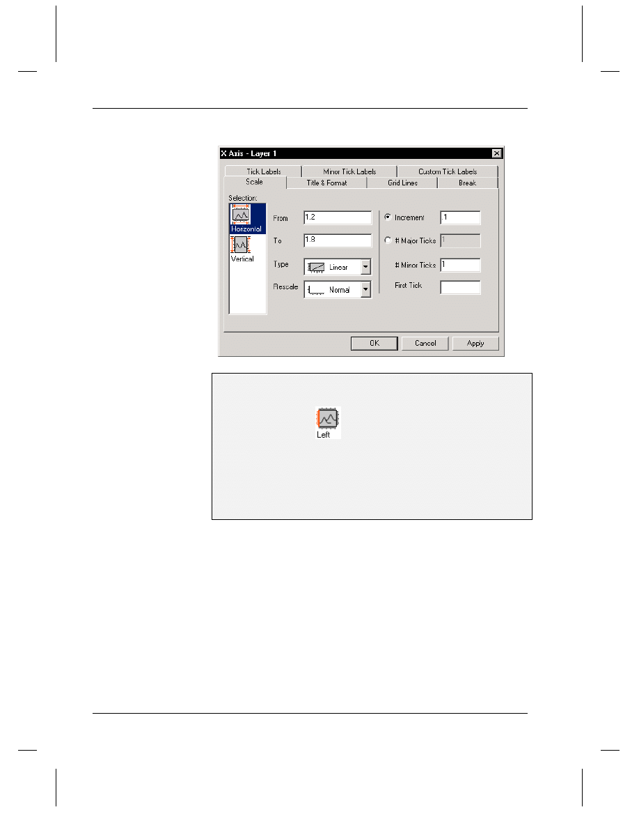
Tutorial 1, Plotting Your Data

•

Customizing the Graph

Figure 10: The X Axis Dialog Box

3) Select the Title & Format tab.
4) Type Time (sec) in the Title text box, overtyping the default text.

5) Select the Left icon

from the Selection list box.

6) Type Potential (mV) in the Title text box, overtyping the default text.
7) Select the Scale tab.
8) Type -.001 in the From text box, .014 in the To text box, and .002 in
the Increment text box.
9) Click OK.

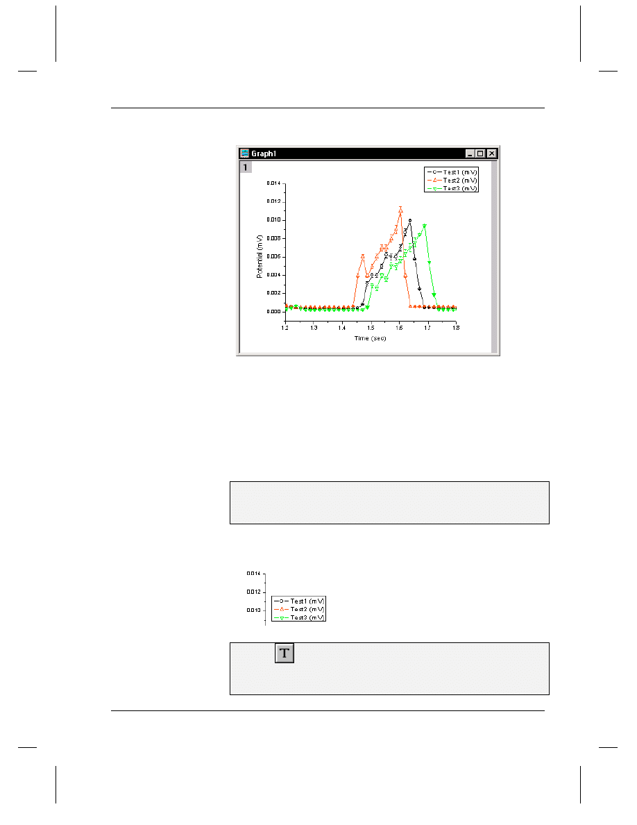
Tutorial 1, Plotting Your Data

Customizing the Graph

•

Figure 11: Customizing the Graph

Adding Text to the Graph

To further customize your graph, you can add annotations including text,
arrows, lines, and shapes. The tools that let you add these annotations
are located on the Tools toolbar. Alternatively, you can right-click
anywhere in the graph to add text using a shortcut menu.

To Add Text to the Graph:
1) First click and drag the legend so that it is located close to the Y axis.
Click off the legend to de-select it.

Figure 12: Moving the Legend

2) Click

on the Tools toolbar and then click in the upper-left

position of the graph. The cursor begins flashing where you clicked.
3) Type Effect of Solvent Loss on Sample Potential.

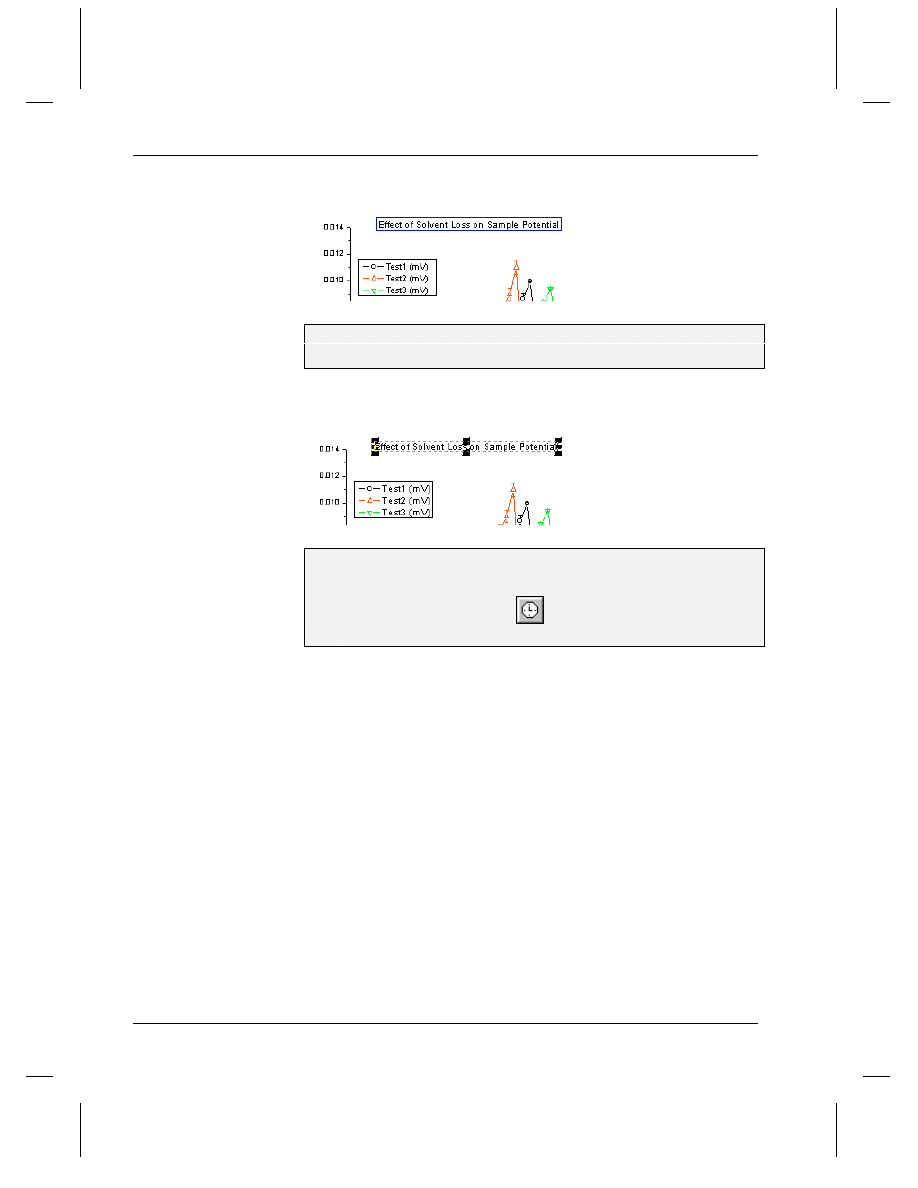
Tutorial 1, Plotting Your Data

•

Customizing the Graph

Figure 13: In-place Text Editing

4) Press ESC to exit the text editing mode.
5) Click once on the new text label so that it becomes selected.

Figure 14: Selecting the Text Label

6) Drag the bottom right control handle to increase the size of the label.
7) Click off the label when done.

8) Click the Date & Time button

on the Graph toolbar to add a date

and time stamp.

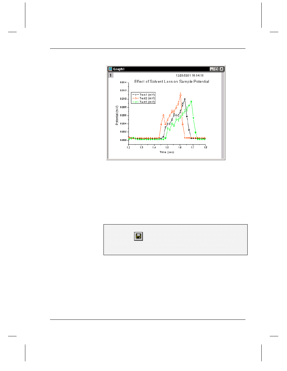
Tutorial 1, Plotting Your Data

Saving Your Project

•

Figure 15: The Finished Graph

Saving Your Project

Your project currently consists of one worksheet and one graph window
and the data displayed in both. Both of these windows and the data they
contain are saved within an Origin project file when you save the project.

To Save Your Project:

1) Click Save

on the Standard toolbar.

2) Type Tutorial_1 in the File Name text box, then click Save. The
project is saved as Tutorial_1.OPJ.

Tutorial 1, Plotting Your Data

•

Saving Your Project

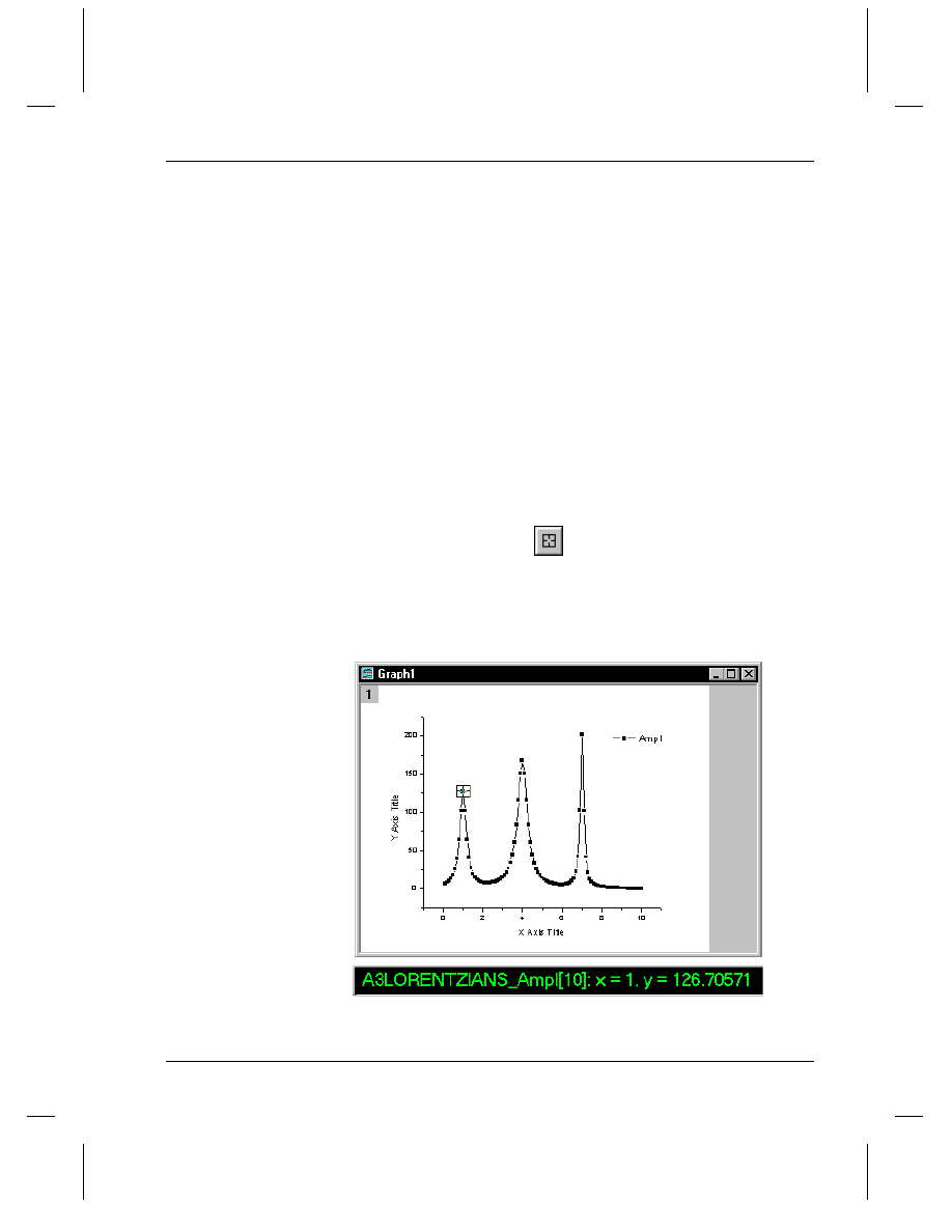
Tutorial 2, Exploring Your Data

Introduction

•

Tutorial 2, Exploring Your Data

Introduction

Origin offers a number of tools to select a region of a data plot, view
coordinate or screen values, enhance the data plot display, and mask data.

Data Reader

To read the X, Y, and Z (for 3D and contour) values for a data point,

click the Data Reader button

on the Tools toolbar. This action

opens the Data Display tool if it is not already open. Click on the desired
data point to read its X,Y, and Z coordinates in the Data Display tool.

Figure 1: Using the Data Reader Tool

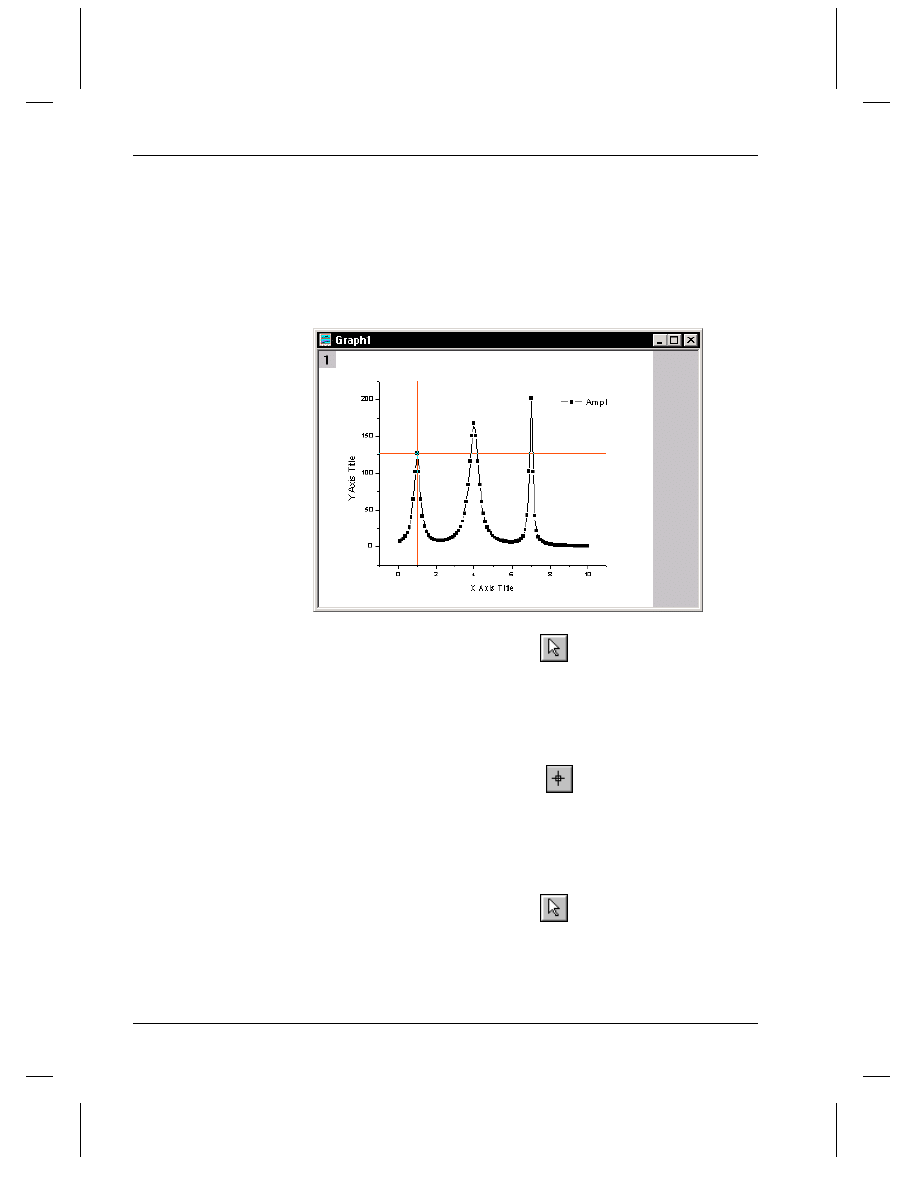
Tutorial 2, Exploring Your Data

100

•

Introduction

To move the cross-hair to the next data point along the data plot, use the
left and right arrow keys or click on the data point.
To change the vertical and horizontal cross hair size after clicking on a
point, press the spacebar. Continue pressing the spacebar to further
increase the size of the cross hairs.

Figure 2: Increasing the Cross Hair Size

Press ESC or click the Pointer button

on the Tools toolbar when you

are finished.

Screen Reader

To read the X, Y, and Z (for 3D and contour) values for any point on the

screen, click the Screen Reader button

on the Tools toolbar. This

action opens the Data Display tool if it is not already open. Click on the
desired screen location to read its X,Y, and Z coordinates in the Data
Display tool.
As with the Data Reader tool, you can press the spacebar to increase the
cross hair size.

Press ESC or click the Pointer button

on the Tools toolbar when you

are finished.

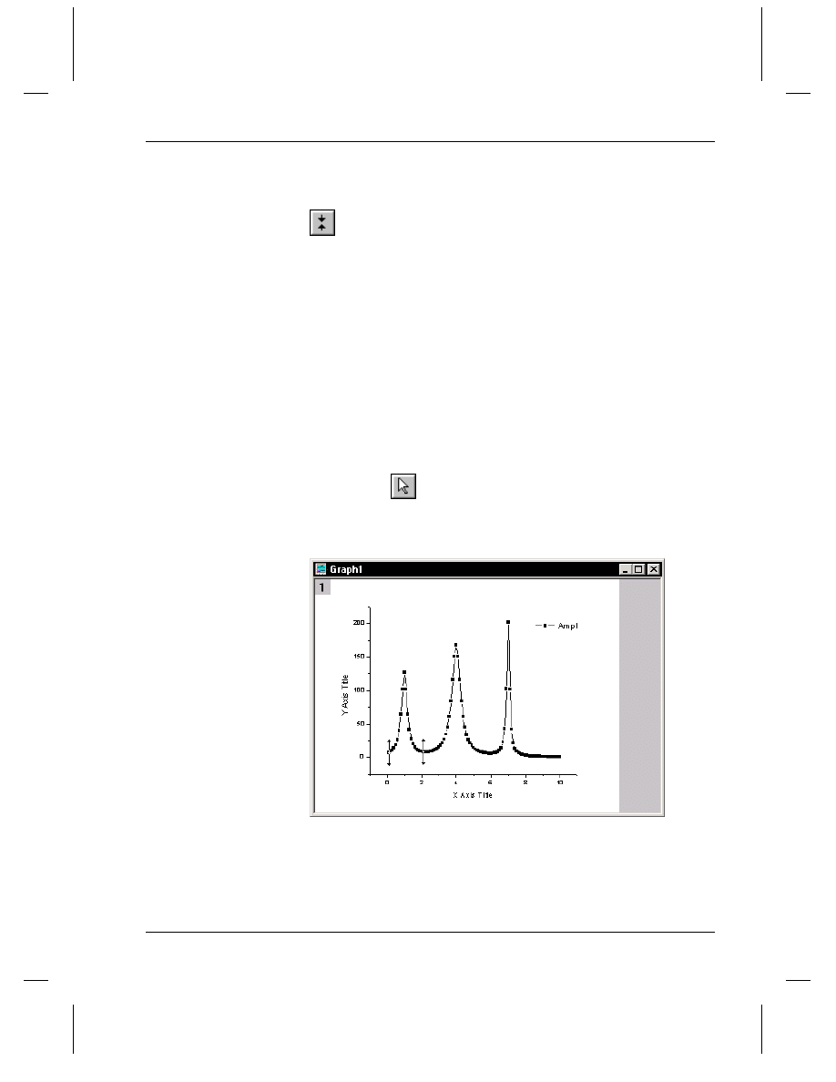
Tutorial 2, Exploring Your Data

Introduction

•

101

Data Selector

To select a range of a data plot for analysis, click the Data Selector tool

on the Tools toolbar. Data markers display at both ends of the

active data plot. Additionally, the Data Display tool opens if it is not
already open.
To mark the data segment of interest, click and drag the markers with the
mouse. You can also use the left and right arrow keys to select a marker.
The CTRL + left or right arrow keys move the selected marker to the
next data point. Holding both the SHIFT and CTRL keys while
depressing the left or right arrow keys moves the data markers in
increments of five along the data plot. (Note: If your X data is not
sorted, you may need to sort the data before selecting a range. To do
this, activate the worksheet and select Analysis:Sort
Worksheet:Ascending.)
As with the Data Reader tool, you can press the spacebar to increase the
cross hair size.
After you have defined the range of interest, press ESC or click the

Pointer button

on the Tools toolbar.

Figure 3: Selecting a Range of Data for Analysis

Any analysis operations you perform on this data plot will apply to the
selected region only.

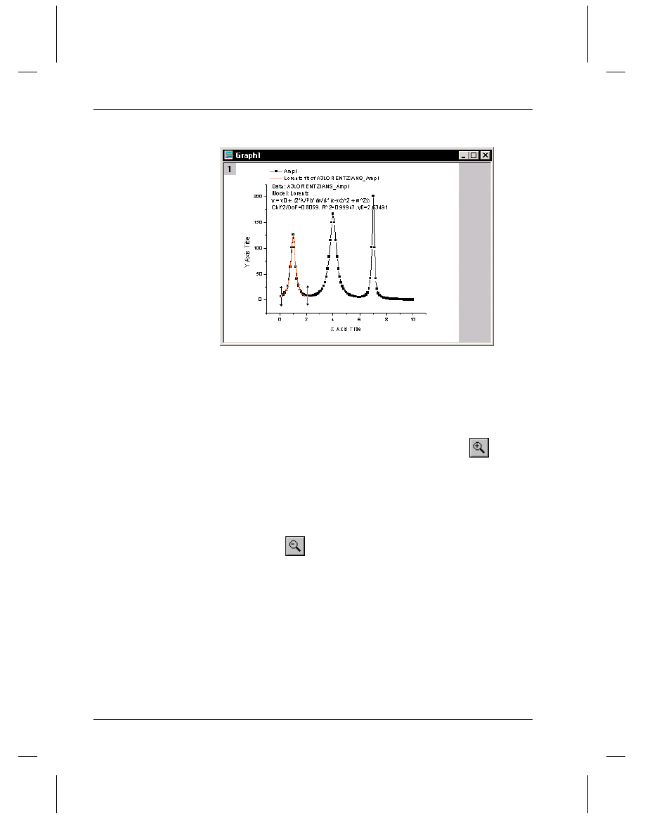
Tutorial 2, Exploring Your Data

102

•

Introduction

Figure 4: Performing a Fit in the Selected Range

To hide the data outside this range, select Data:Set Display Range.
To remove the selection range, select Data:Reset to Full Range.

Enlarger Tool and Undo Enlarge

To magnify a portion of a data plot, click the Enlarger tool

on the

Tools toolbar. The close-up of the data can be viewed in the current
window or in a new window. When a data plot is magnified using the
Enlarger tool, the axes are rescaled to show an expanded view of the
data.
=> To view the magnified data in the current window, drag the area of
interest in the graph. To re-display the entire data plot, click the Undo

Enlarge button

=> To view the magnified data in a new window, hold down the CTRL
key while dragging the area of interest in the graph window. Release the
mouse button, then release the CTRL key. Origin opens a new graph
window named Enlarged. A rectangle object with sizing handles appears
in the original graph window (if the sizing handles are not displayed,
click on the object to select it).

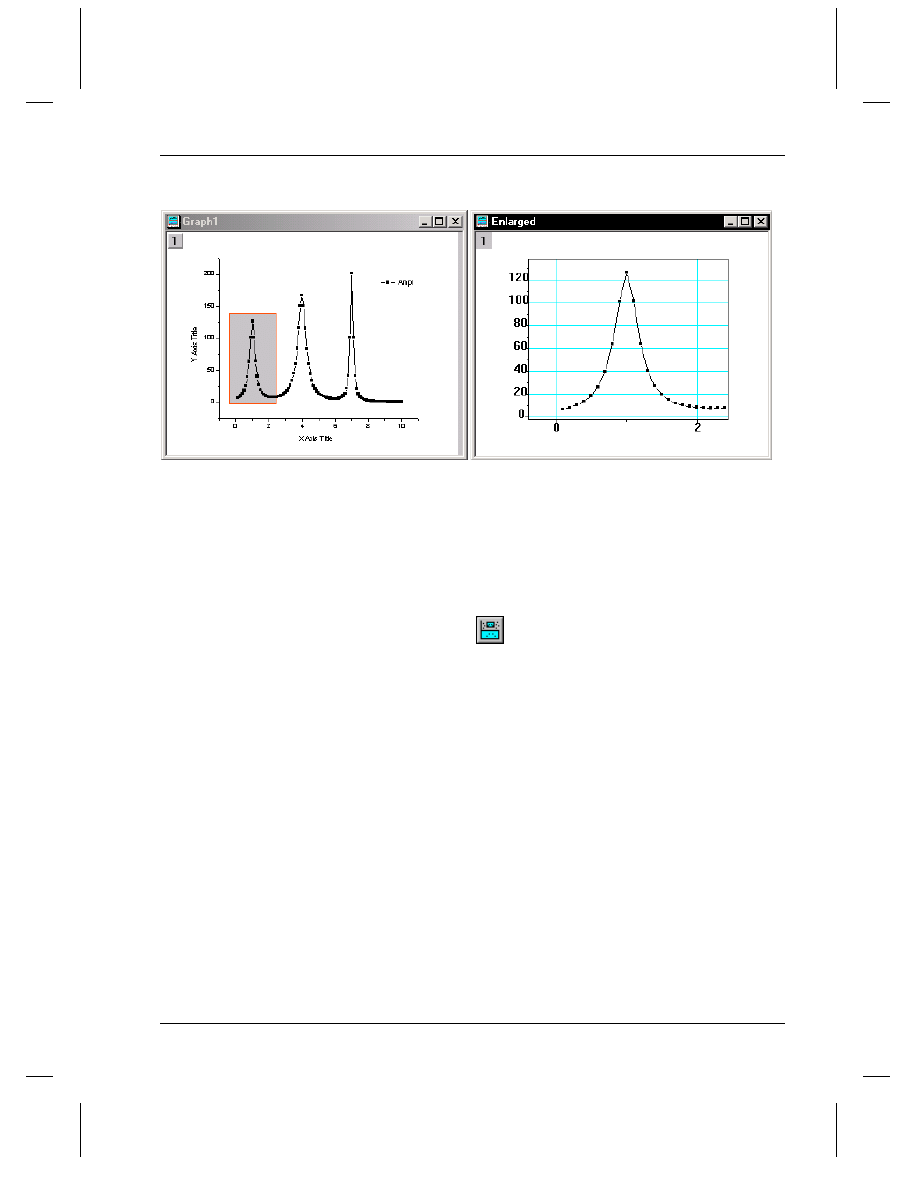
Tutorial 2, Exploring Your Data

Introduction

•

103

Figure 5: Viewing the Data in the Enlarged Window

To change the data segment in the Enlarged window, resize the
rectangular object or change its position by dragging in the original graph
window. The Enlarged window updates accordingly.
After you finish analyzing the data, you can click on the rectangle object
and delete it.
=> To view the magnified data in the same graph window (along with
the full range of data), highlight the desired worksheet column(s) and

click the Zoom button

on the 2D Graphs Extended toolbar. A graph

window with two layers opens. The top layer displays the entire data
range and the bottom layer provides a zoomed-in view of your data plot.

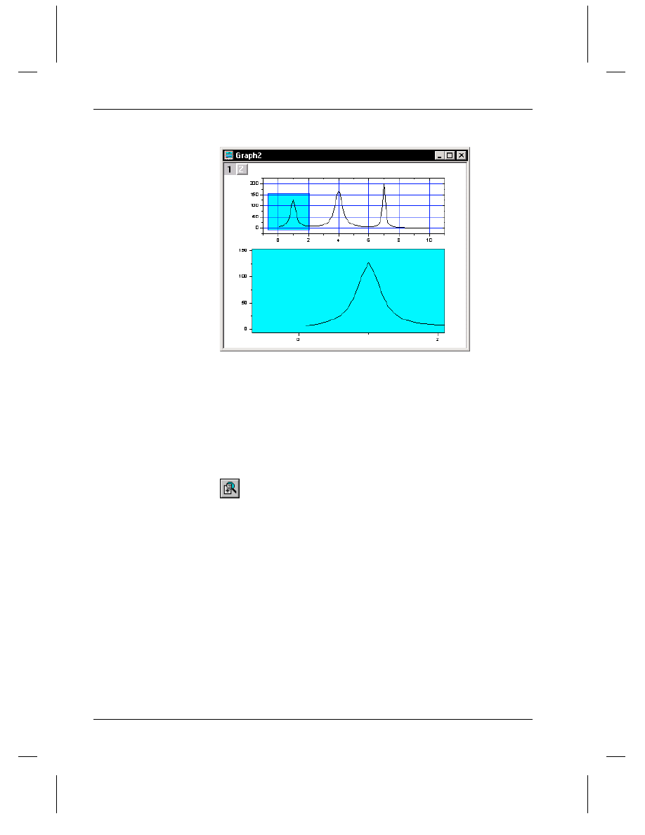
Tutorial 2, Exploring Your Data

104

•

Introduction

Figure 6: Viewing the Full and Enlarged Range Together

To change the data segment in the bottom layer, resize the rectangular
object or change its position by dragging in the top layer.
After you finish analyzing the data, you can click on the rectangle object
and delete it.

Zoom In and Zoom Out

To display a close-up view of the graph page, click the Zoom In button

on the Graph toolbar, then click on the desired zoom location in the

graph window. Origin zooms the page, centering the zoom view at this
location in the window (the axes are not rescaled).

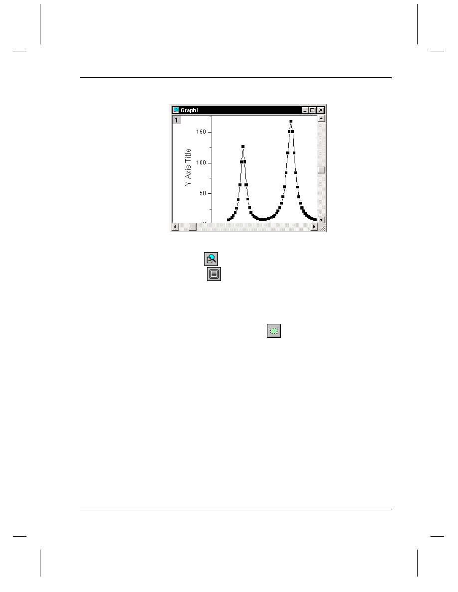
Tutorial 2, Exploring Your Data

Introduction

•

105

Figure 7: Zooming in on the Graph

To zoom in closer, click the button again. To zoom out, click the Zoom

Out button

. To return the view to the full page, click the Whole

Page button

Region of Interest (Image Data)

When you import image data in a matrix, you can select a region of the

image using the Rectangle Tool

on the Tools toolbar. (When a

matrix with an image is active, the Rectangle tool displays in the "region
of interest mode" by default. This setting is controlled from the
Tools:Region of Interest Tools menu command.) Select the Rectangle
Tool and then drag your region of interest. Then right-click in this region
and select Crop, Copy, or Create New from the shortcut menu.

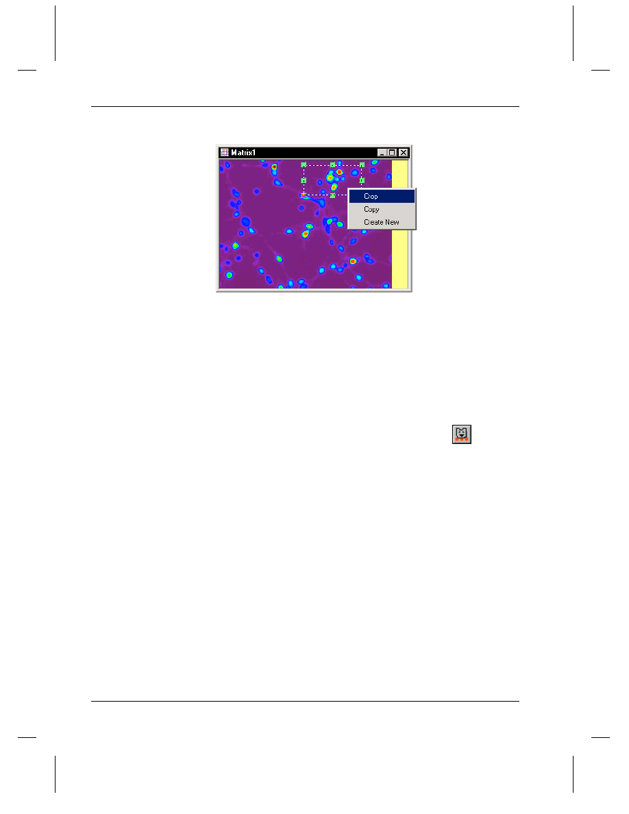
Tutorial 2, Exploring Your Data

106

•

Introduction

Figure 8: Selecting a Region of Interest in an Image

Masking

Select View:Toolbars
if the Mask toolbar
isn't open.

The Mask toolbar allows you to exclude ranges of data or individual
data points from analysis. It is most useful if you want to analyze only a
specific section of your data, or if you have erroneous data points that
you do not want included in your analysis. The Mask toolbar is
available for both worksheet and graph windows. For graph windows,
masking is only available for scatter or line + symbol graphs.

To mask a range in a graph, click the Mask Range button

. Then

move the data markers so that they define the range you want to mask.

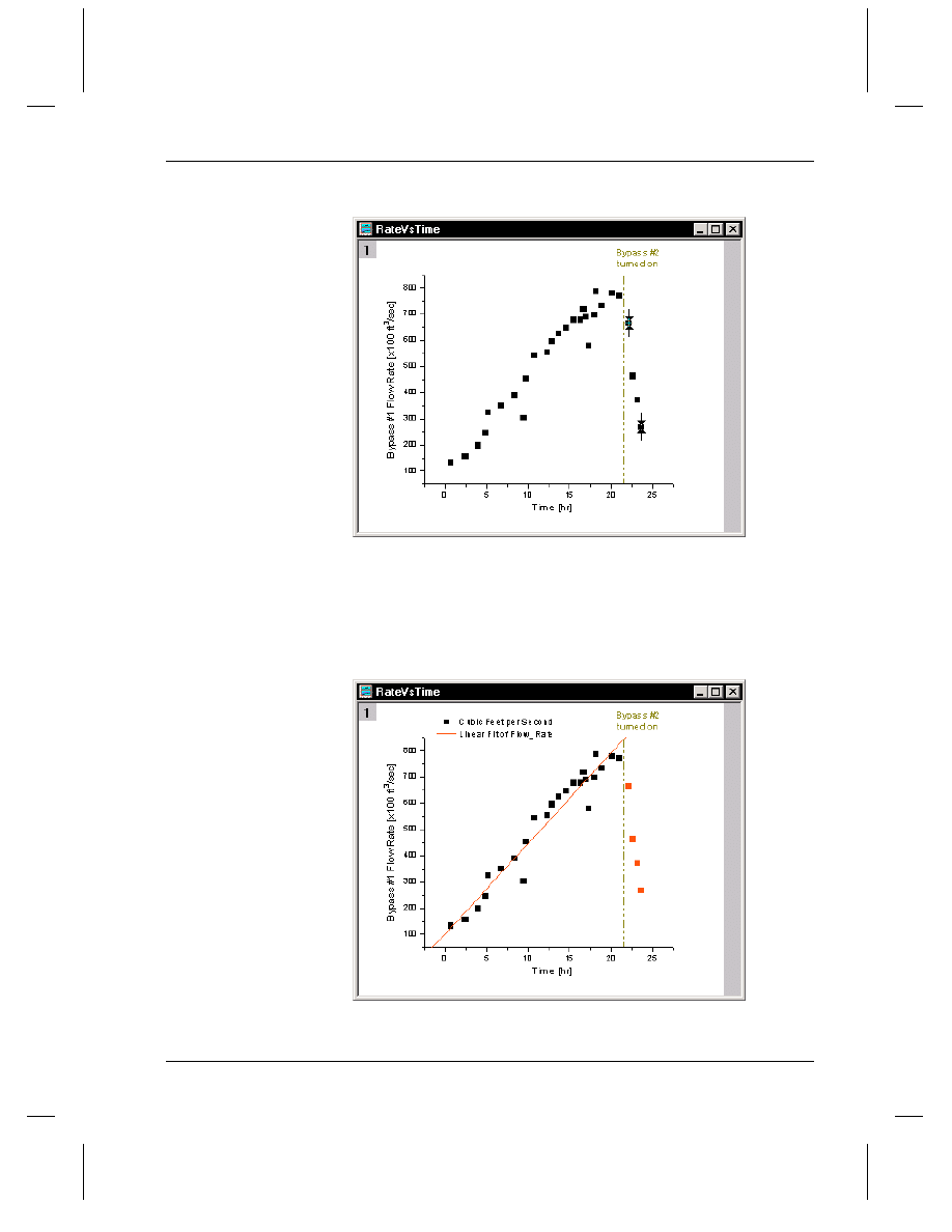
Tutorial 2, Exploring Your Data

Introduction

•

107

Figure 9: Masking a Range of Data

When finished defining the range, press ENTER. The masked points
then display with red color. Any analysis you perform on this data plot
will exclude the masked data.

Figure 10: Linear Fit Excluding the Masked Region

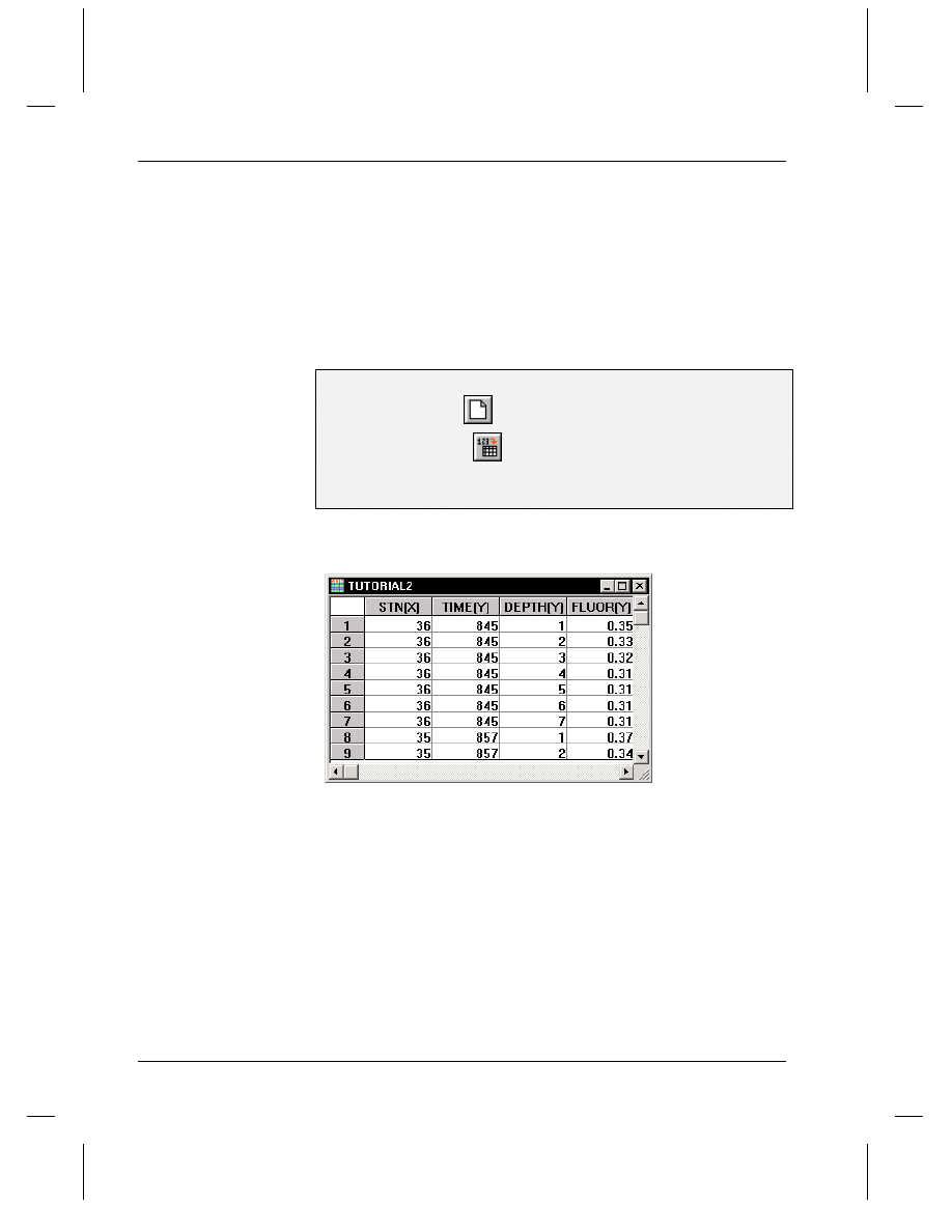
Tutorial 2, Exploring Your Data

108

•

Getting Started

The following tutorial will show you more about using the masking tools.
It will also show you how to mathematically transform data in a
worksheet column, sort a worksheet based on primary and secondary
columns, and plot a range of worksheet data.
To begin this tutorial, you will open a new Origin project and import
ASCII data.

To Import the Data File:

1) Click New Project

on the Standard toolbar.

2) Click Import ASCII

, then select TUTORIAL_2.DAT from the

Origin \TUTORIAL folder.
3) Click Open.

Figure 11: Importing the ASCII File

Note: There are several columns that are not visible due to the current
worksheet size. When there is a reference in this tutorial to a column that
is not visible, scroll the worksheet to locate it.

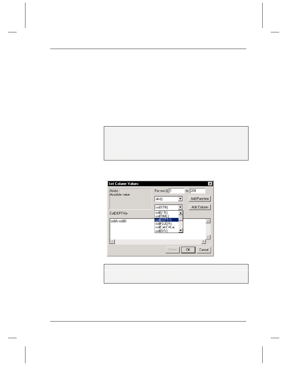
Tutorial 2, Exploring Your Data

Transforming Column Values

•

109

Transforming Column Values

You can also include
compiled Origin C
functions in the Set
Column Values dialog
box.

You can create or transform data sets using any mathematical expression
recognized by Origin in the Set Column Values dialog box. This dialog
box provides a text box for you to type a value or mathematical
expression to apply to the selected column or range of the column. It
also includes a function drop-down list from which you can select a
function to add to the text box. In addition, a column drop-down list
contains a list of all the columns in the active worksheet. Select the
column you want to add to the text box, then click Add Column to add
the selected column to the text box.

To Transform the Column Values:
1) Right-click on the Depth(Y) column heading.
2) Select Set Column Values from the shortcut menu.
3) Leave col(A)-col(B) highlighted in the text box and select
col(DEPTH) from the Add Column drop-down list.

Figure 12: Selecting the Depth Column

4) Click Add Column. Col(DEPTH) overwrites the highlighted text.
5) Leave the cursor at the current location in the text box and type
*.3048 in the text box.

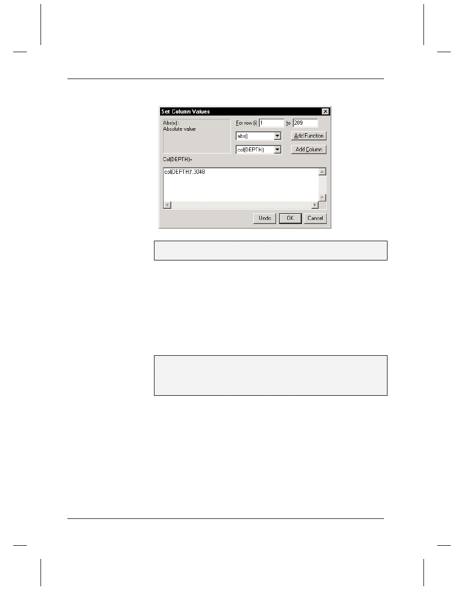
Tutorial 2, Exploring Your Data

110

•

Sorting Worksheet Data

Figure 13: Transforming the Column Values

6) Click OK. The expression you typed in the Set Column Values
dialog box is used to update the values in the DEPTH column.

Sorting Worksheet Data

Origin can sort individual columns, multiple selected columns, or entire
worksheets. Origin offers simple sorting in which specified data is sorted
using one "sort by" column and a selected sort order, as well as nested
sorting.

To Sort the Worksheet Data:
1) Move the mouse pointer to the upper-left corner of the worksheet to
turn the cursor into a downward pointing arrow, then click to select all
the columns in the worksheet.

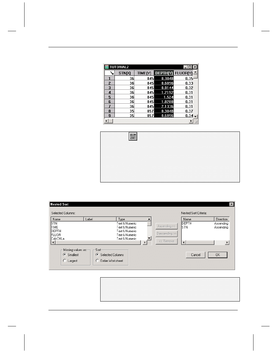
Tutorial 2, Exploring Your Data

Sorting Worksheet Data

•

111

Figure 14: Positioning the Cursor to Select All Columns

2) Click Sort

on the Worksheet Data toolbar to open the Nested

Sort dialog box.
3) Select DEPTH from the Selected Columns list box, then click
Ascending. The column is added to the Nested Sort Criteria list box.
This selection makes DEPTH the primary sort column in ascending
order.
4) Select STN from the Selected Columns list box, then click Ascending.
This makes STN the secondary sort column in ascending order.

Figure 15: Sorting the Worksheet

5) Click OK.
6) De-select the worksheet by clicking in the upper–left blank space in
the worksheet (without the cursor changing to the downward pointing
arrow).

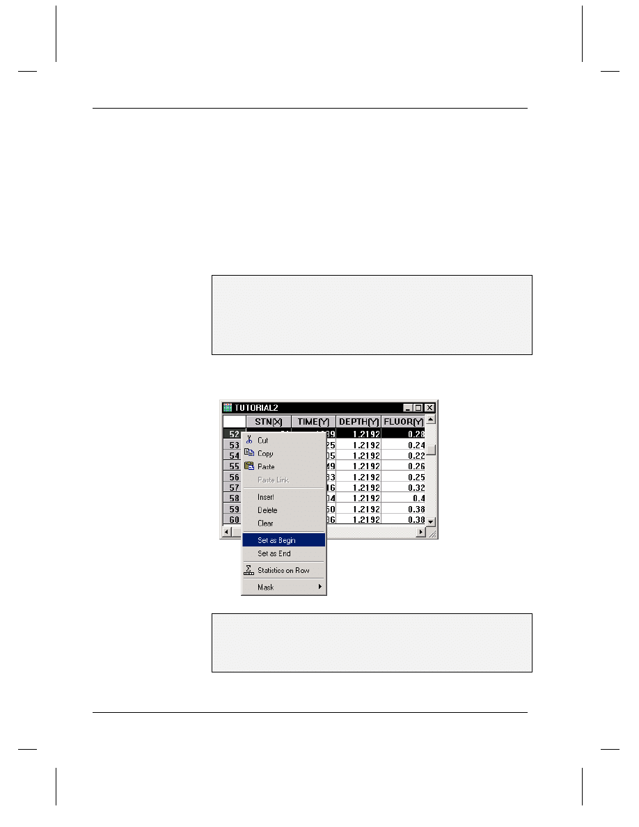
Tutorial 2, Exploring Your Data

112

•

Plotting a Range of the Worksheet Data

The entire worksheet is sorted so that the values in the DEPTH (primary)
column are ascending. If there are two cells of equal value in the
DEPTH column, then the values in the corresponding rows of the STN
(secondary) column are used to determine the worksheet order.

Plotting a Range of the Worksheet Data

You can set the worksheet display range so that subsequent plotting and
analysis are performed only on the data of interest.

To Select a Range of the Worksheet Data:
1) Select View:Go To Row.
2) Type 52 in the dialog box that opens, then click OK.
3) Right-click on the row heading for row number 52.
4) Select Set As Begin from the shortcut menu.

Figure 16: Selecting a Range of Worksheet Data

5) Use the vertical scroll bar to move down in the worksheet so that row
number 68 is visible.
6) Right-click on the row heading for row number 68.
7) Select Set As End from the shortcut menu.

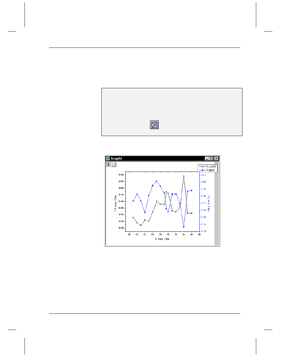
Tutorial 2, Exploring Your Data

Masking Data in the Graph

•

113

Notice that the data outside the selected range is no longer displayed in
the worksheet. The data has not been deleted from the worksheet, only
hidden to provide for easier viewing of the selected range. The hidden
data can be shown by re-selecting the entire worksheet and then selecting
Edit:Reset to Full Range.

Plotting the Data:
1) Click the FLUOR column heading to select the column.
2) Scroll to the right in the worksheet and CTRL+click on the TEMP
column heading. This selects the TEMP column while leaving the
FLUOR column selected.

3) Click Double Y Axis

on the 2D Graphs Extended toolbar.

(Select View:Toolbars if the 2D Graphs Extended toolbar isn't open.)

Figure 17: Plotting a Range of Worksheet Data

Masking Data in the Graph

The Mask toolbar is provided for excluding data from Origin's analysis
and fitting routines. You can mask individual data points or a range of
data. Once data is masked, options become available to change the
masked data color, hide or show the masked data, swap the masked and
unmasked data, and enable or disable masking.

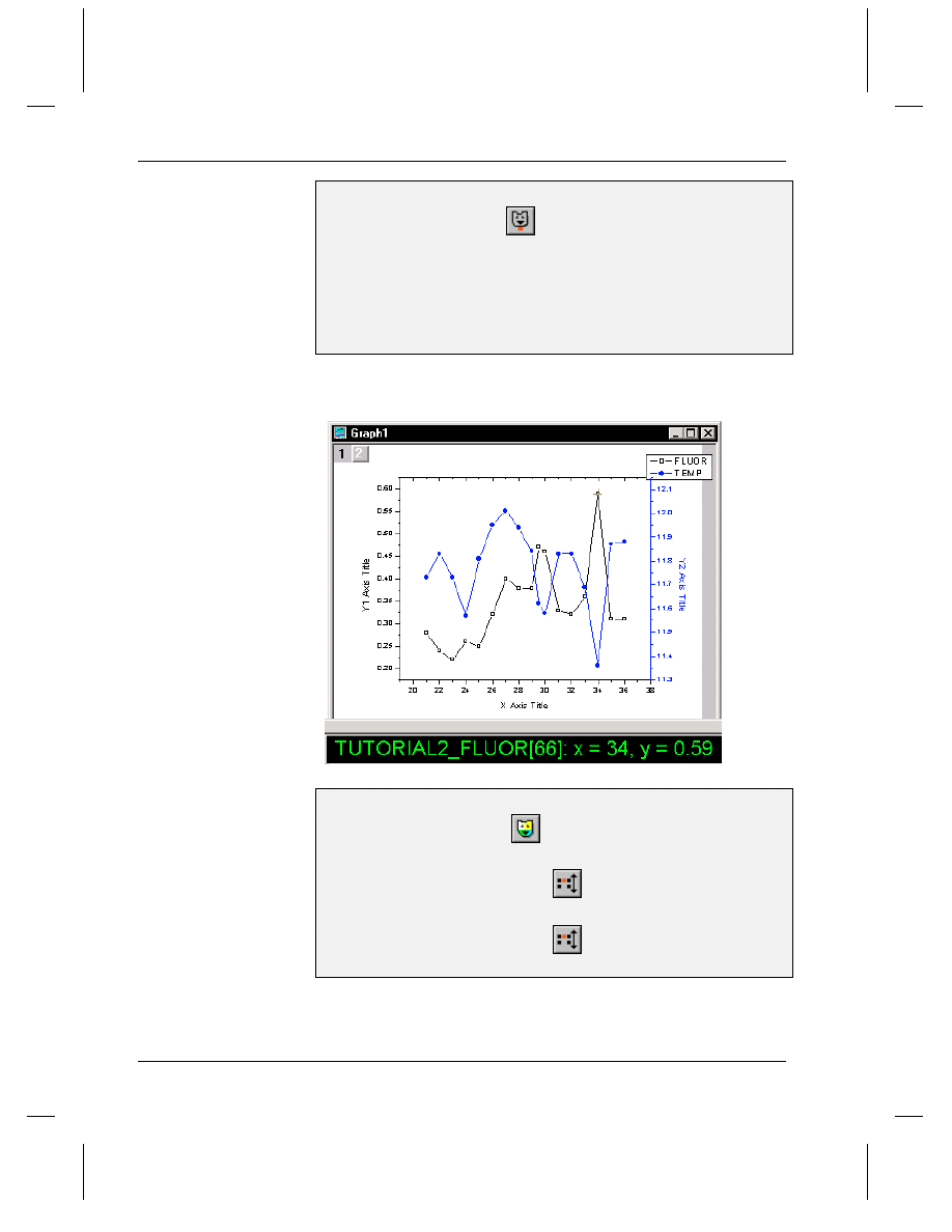
Tutorial 2, Exploring Your Data

114

•

Masking Data in the Graph

To Mask a Data Point in the Graph:

1) Click Mask Point Toggle

on the Mask toolbar. (Select

View:Toolbars if the Mask toolbar isn't open.) This activates the Data
Reader tool.
2) Click on the FLUOR data plot in the graph (black, open square
symbols) and then use the right or left arrows on the keyboard to move
the cursor to the data point at X = 34 and Y = .59. The Data Display tool
displays the current coordinate values.

Figure 18: Masking Data in the Graph Window

3) Press ENTER to select this point for masking.

4) Click Change Mask Color

on the Mask toolbar. The color

changes to green.

5) Click Hide/Show Masked Points

on the Mask toolbar to hide the

masked data point.

6) Click Hide/Show Masked Points

on the Mask toolbar again to

show the data point.

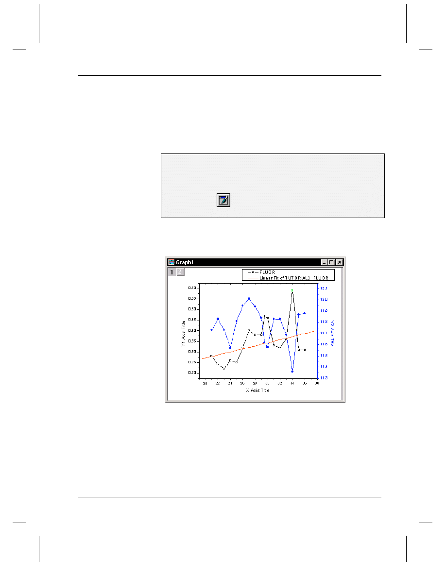
Tutorial 2, Exploring Your Data

Performing a Linear Fit on the FLUOR Data Plot

•

115

Performing a Linear Fit on the FLUOR Data Plot

Now that a data point is masked in the FLUOR data plot, subsequent
analysis and fitting are performed only on the non-masked data. You
can, however, disable the mask on the data point, and analyze or fit all
the data points in the current selection range.

To Perform a Linear Fit with the Data Point Masked:
1) Select Analysis:Fit Linear. A fit line is added to the graph and the
Results Log opens displaying the fitting results. You can scroll the
Results Log to view the results.

2) Click Refresh

on the Standard toolbar and reposition the legend

so it fits on the page.

Figure 19: Linear Fit of the FLUOR Data Plot with a Masked Data
Point

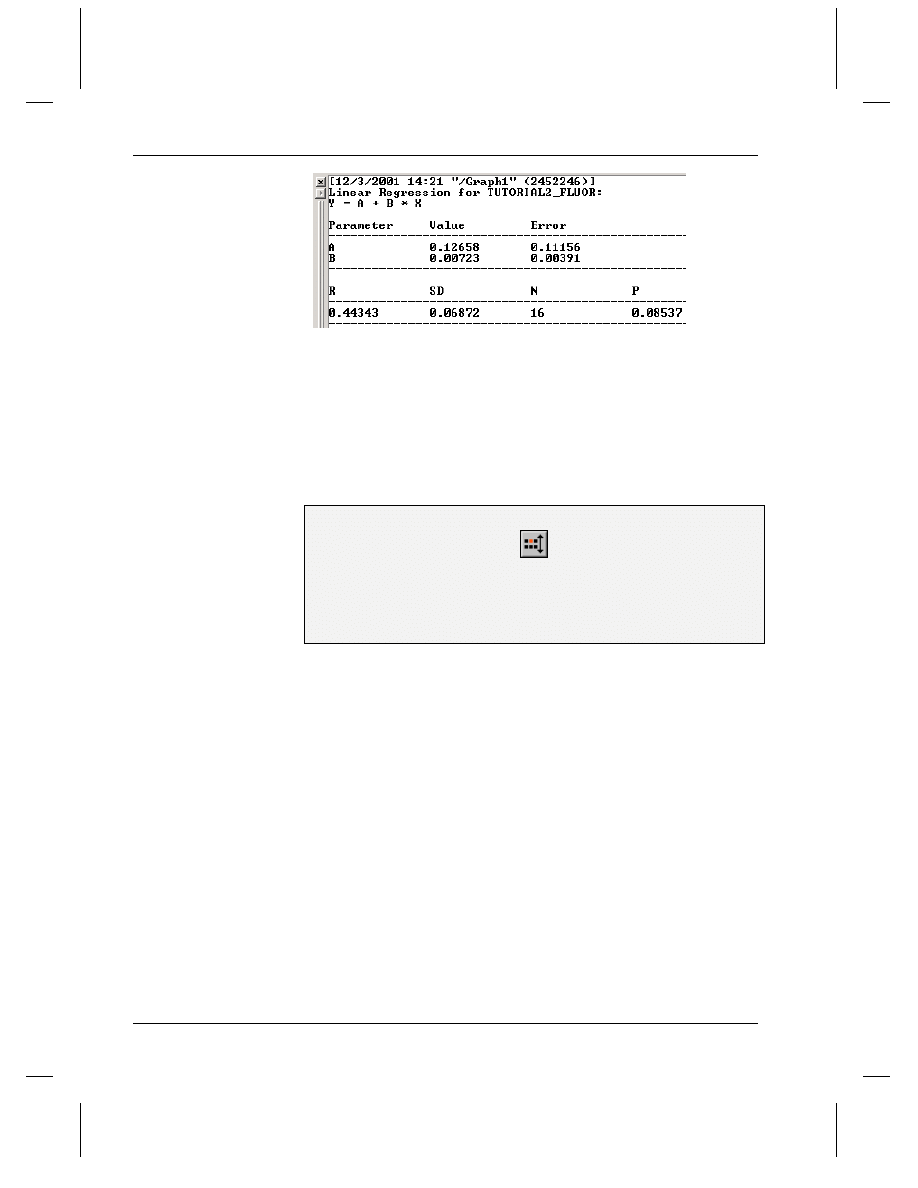
Tutorial 2, Exploring Your Data

116

•

Performing a Linear Fit on the FLUOR Data Plot

By default, the Results Log shows the results for all fitting done in the
currently active Project Explorer folder. To change this default behavior,
right-click in the Results Log and select a different viewing option.
Each time a new fit is done the results are appended to the Results Log.
Each entry in the Results Log includes a date/time stamp, the window
name, a numeric stamp which is the Julian day, the type of analysis
performed, and the results.

To Perform a Linear Fit with the Mask Disabled:

1) Click Disable/Enable Masking

on the Mask toolbar. The

masked data point changes from green to black.
2) Select Analysis:Fit Linear. A second fit line is drawn on the graph.
3) Verify that the mask is disabled by comparing the two fit results in
the Results Log.

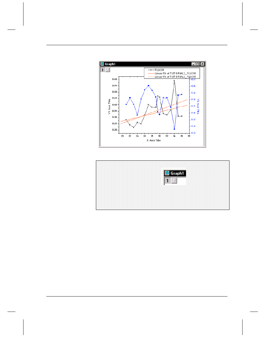
Tutorial 2, Exploring Your Data

Performing a Linear Fit on the FLUOR Data Plot

•

117

Figure 20: Linear Fit of Data with Mask Disabled (2 Fit Lines)

To Remove the First Fit Line From the Graph:

1) Double-click on the layer 1 icon

in the upper-left

corner of the graph. This opens the Layer 1 dialog box.
2) Select linearfit1_tutorial2fluo from the Layer Contents list box.
3) Click the <= arrow (to the left of the Layer Contents list box). The
data set is removed from the list box.

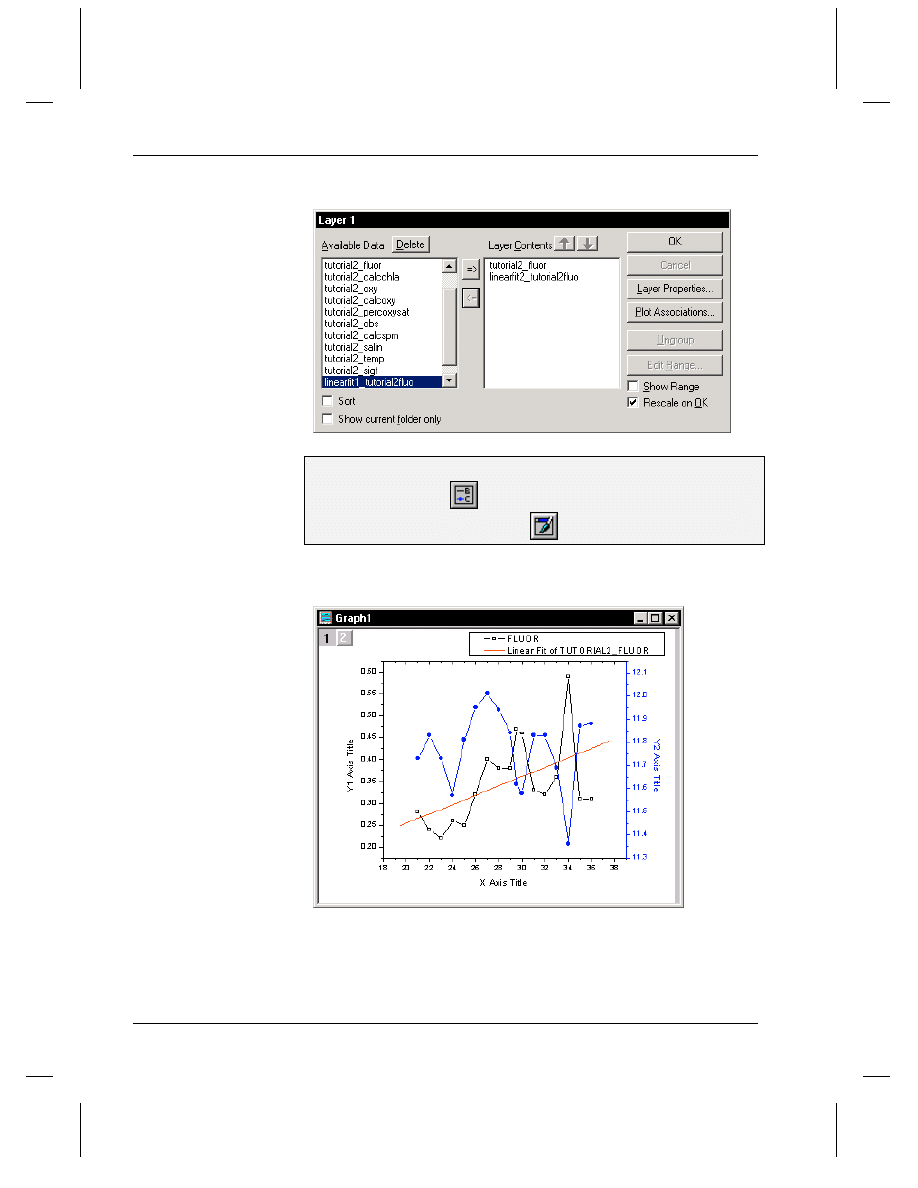
Tutorial 2, Exploring Your Data

118

•

Performing a Linear Fit on the FLUOR Data Plot

Figure 21: Removing the First Fit Line from the Graph

4) Click OK to close the dialog box.

5) Click New Legend

on the Graph toolbar to update the legend.

You may need to also click Refresh

on the Standard toolbar.

Figure 22: Linear Fit of Data with Mask Disabled (1 Fit Line)

Tutorial 2, Exploring Your Data

Saving the Project

•

119

Saving the Project

Your Origin project currently consists of your data, worksheets, graph,
analysis results and the current folder organization in the Project
Explorer.

To Save the Project:
1) Select File:Save Project.
2) Type a name in the File Name text box.
3) Click Save.

Tutorial 2, Exploring Your Data

120

•

Saving the Project

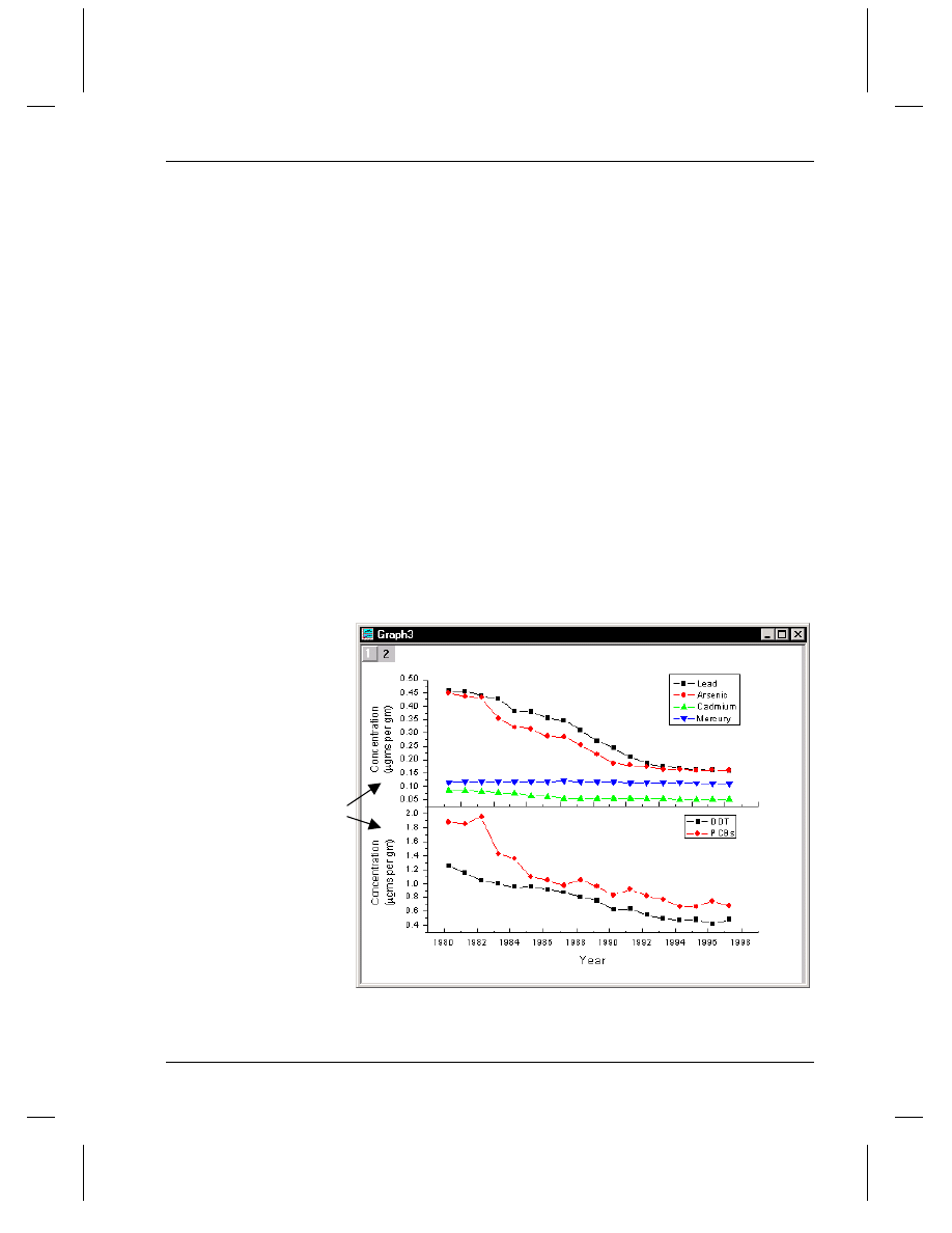
Tutorial 3, Creating Multiple Layer Graphs

Introduction

•

121

Tutorial 3, Creating Multiple

Layer Graphs

Introduction

The layer is the fundamental building block of Origin graphs. A layer is
an Origin object consisting of one set of controlling axes. Furthermore,
any, none, or all of the four axes (the top and bottom X and right and left
Y) that make up the layer may or may not be displayed. A layer can
contain objects, such as labels, or data plots, that also may or may not be
displayed. A graph window must contain at least one layer and may
include as many as 80 layers.

Figure 1: Multiple Layer Graph

2 layers

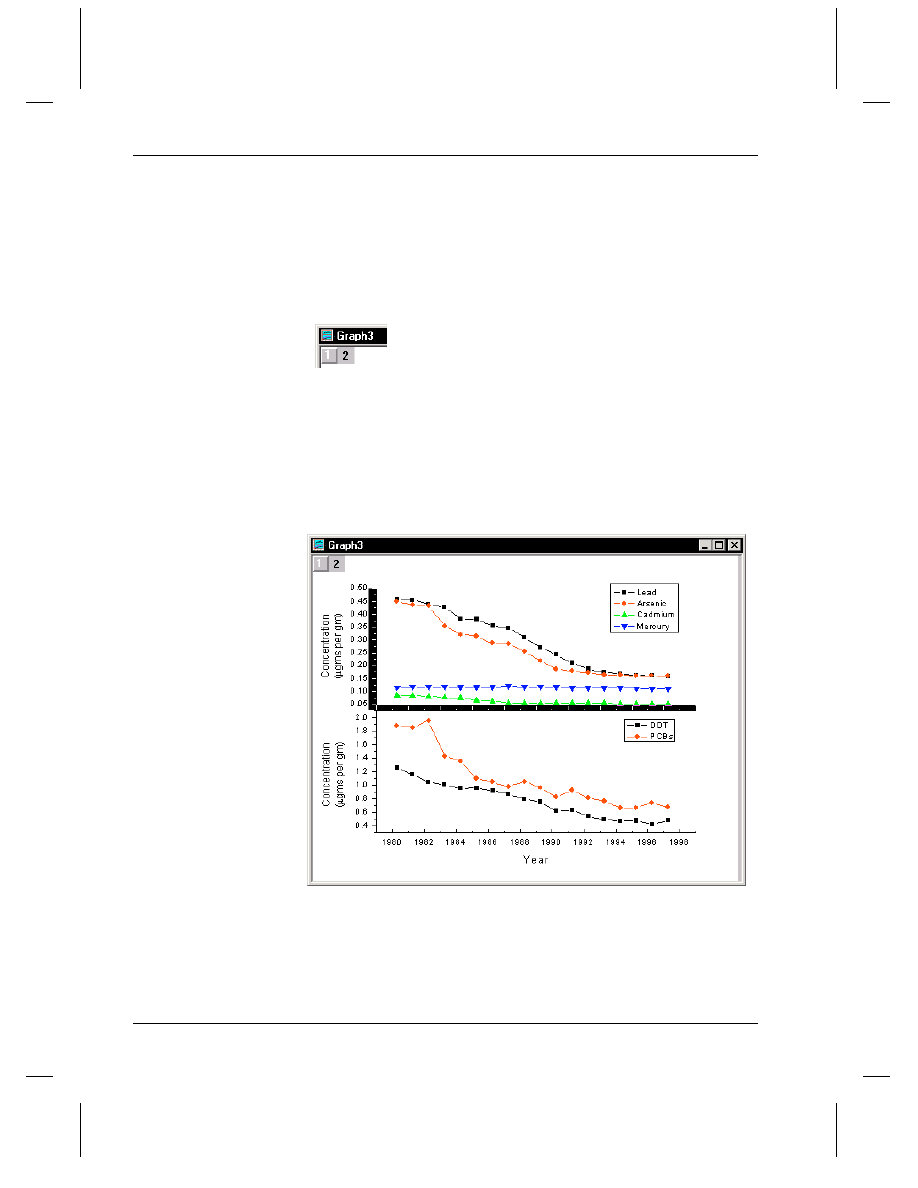
Tutorial 3, Creating Multiple Layer Graphs

122

•

Introduction

There is always one (only one) active layer in a graph window. This
active layer is the only layer that is receptive to program commands. For
example, any data or objects added to a graph will be added to the active
layer. The active layer is denoted by a depressed layer icon in the upper-
left corner of the graph window.

Figure 2: Layer 2 is Active

=> To hide the layer icons, select View:Show:Layer Icons.
=> To highlight the axes in the active layer, select View:Show:Active
Layer Indicator.
Both these actions only effect the currently active graph window.

Figure 3: Highlighting the Axes in the Active Layer

To activate another layer, click the layer icon of the layer you want to be
active.

Tutorial 3, Creating Multiple Layer Graphs

Opening the Project File

•

123

This tutorial will introduce you to Origin's built-in multiple layer graph
templates. It will also show you how to create your own multiple layer
graph and then save it as a template.

Opening the Project File

The data for this tutorial is provided in a project file.

To Open the Project File:

1) Click Open

on the Standard toolbar.

2) In the Origin \TUTORIAL folder, select TUTORIAL_3.OPJ from the
list of files.
3) Click Open. A project containing four graph windows and a
worksheet opens.

Origin's Multiple Layer Graph Templates

Origin contains several built-in, multiple layer graph templates. These
templates allow you to select a range of data, then click a button to plot
the selected data into multiple layers in a graph window.
The double Y axis graph template is ideal for plotting data that includes
two or more dependent data sets and a common independent data set. A
sample double Y axis graph is currently active in your project.

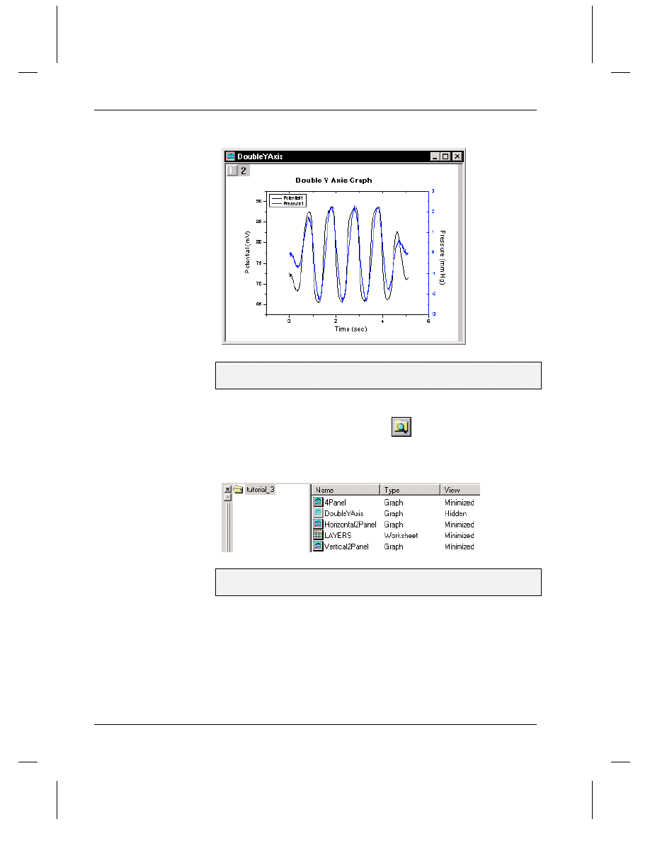
Tutorial 3, Creating Multiple Layer Graphs

124

•

Origin's Multiple Layer Graph Templates

Figure 4: The Double Y Axis Graph

1) Right-click on the double Y axis graph window title bar and select
Hide from the shortcut menu.

Project Explorer provides easy access to all the windows in the project.
By default, Project Explorer is docked at the bottom of your workspace.

If your Project Explorer is closed, click

on the Standard toolbar.

Figure 5: Project Explorer

2) Double-click on the Horizontal2Panel graph icon on the right pane of
Project Explorer.

The horizontal 2 panel graph template is ideal for plotting related data
that does not share an independent data set. You can use the Edit:Add
& Arrange Layers menu command and the Layer tool to customize the
spacing of the layers and to swap the layer arrangement.

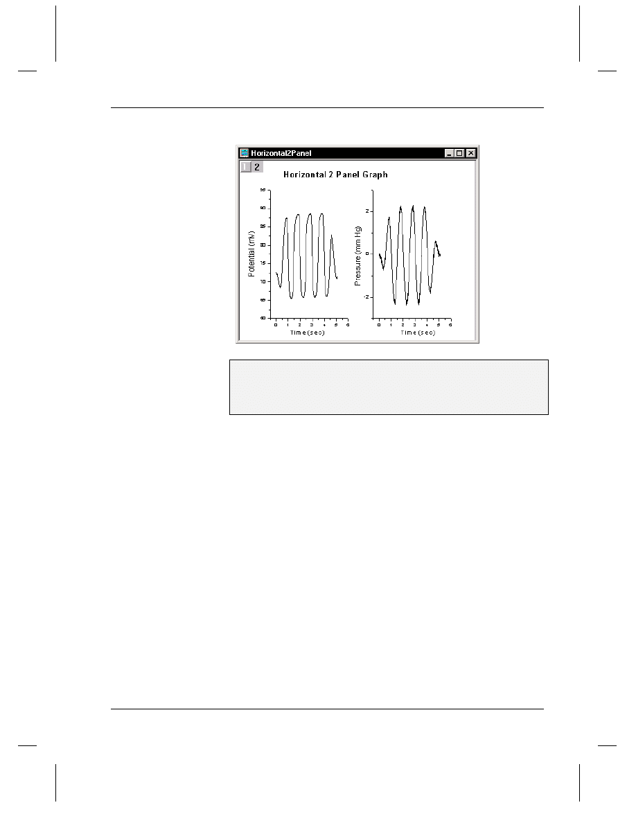
Tutorial 3, Creating Multiple Layer Graphs

Origin's Multiple Layer Graph Templates

•

125

Figure 6: The Horizontal 2 Panel Graph

3) Right-click on the Horizontal2Panel graph icon on the right pane of
Project Explorer and select Hide Window from the shortcut menu.
4) Double-click on the Vertical2Panel graph icon on the right pane of
Project Explorer.

The vertical 2 panel graph template provides the same data presentation
as the horizontal 2 panel graph template, but in a one column with two
rows configuration.

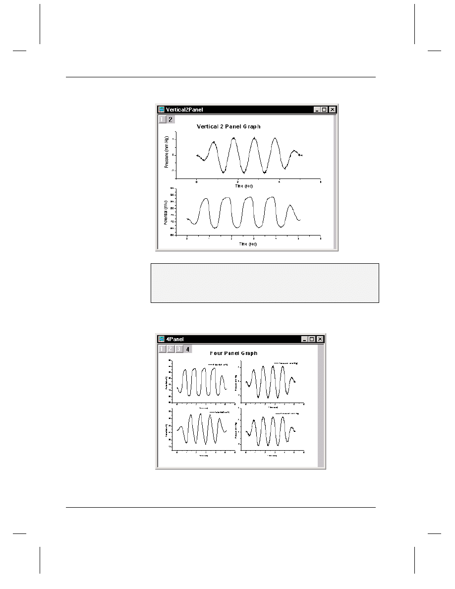
Tutorial 3, Creating Multiple Layer Graphs

126

•

Origin's Multiple Layer Graph Templates

Figure 7: The Vertical 2 Panel Graph

5) Right-click on the Vertical2Panel graph icon on the right pane of
Project Explorer and select Hide Window from the shortcut menu.
6) Double-click on the 4Panel graph icon on the right pane of Project
Explorer.

Figure 8: The 4 Panel Graph

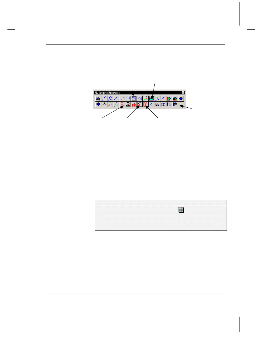
Tutorial 3, Creating Multiple Layer Graphs

Designating Multiple X Columns in the Worksheet

•

127

Additional multiple layer graphs are accessible from the 2D Graphs
Extended toolbar (select your data before clicking the button).

Figure 9: The 2D Graphs Extended Toolbar

Double Y Axis Zoom

QC Chart Histogram+Prob. Stacked Histogram

Panel Graphs

Designating Multiple X Columns in the
Worksheet

When your worksheet includes multiple X columns, Y columns in the
worksheet plot against the nearest X column to the left. Though this
default behavior can be disregarded by selecting non-associated columns
with CTRL selection, the default plotting behavior allows you to quickly
create graphs from associated XY data sets.

To Designate a Second X Column:

1) Double-click on the Layers worksheet icon

on the right pane of

Project Explorer.
2) Right-click on the Trial2 column heading and select Set As:X from
the shortcut menu.

The Trial2 column designation changes to X2 and the columns to the
right of it are designated as Y2. In addition, the Trial1 column
designation changes to X1 and the columns between Trial1 and Trial2 are
designated as Y1. This allows you to quickly determine which column
will be providing the X values for the data you are plotting.

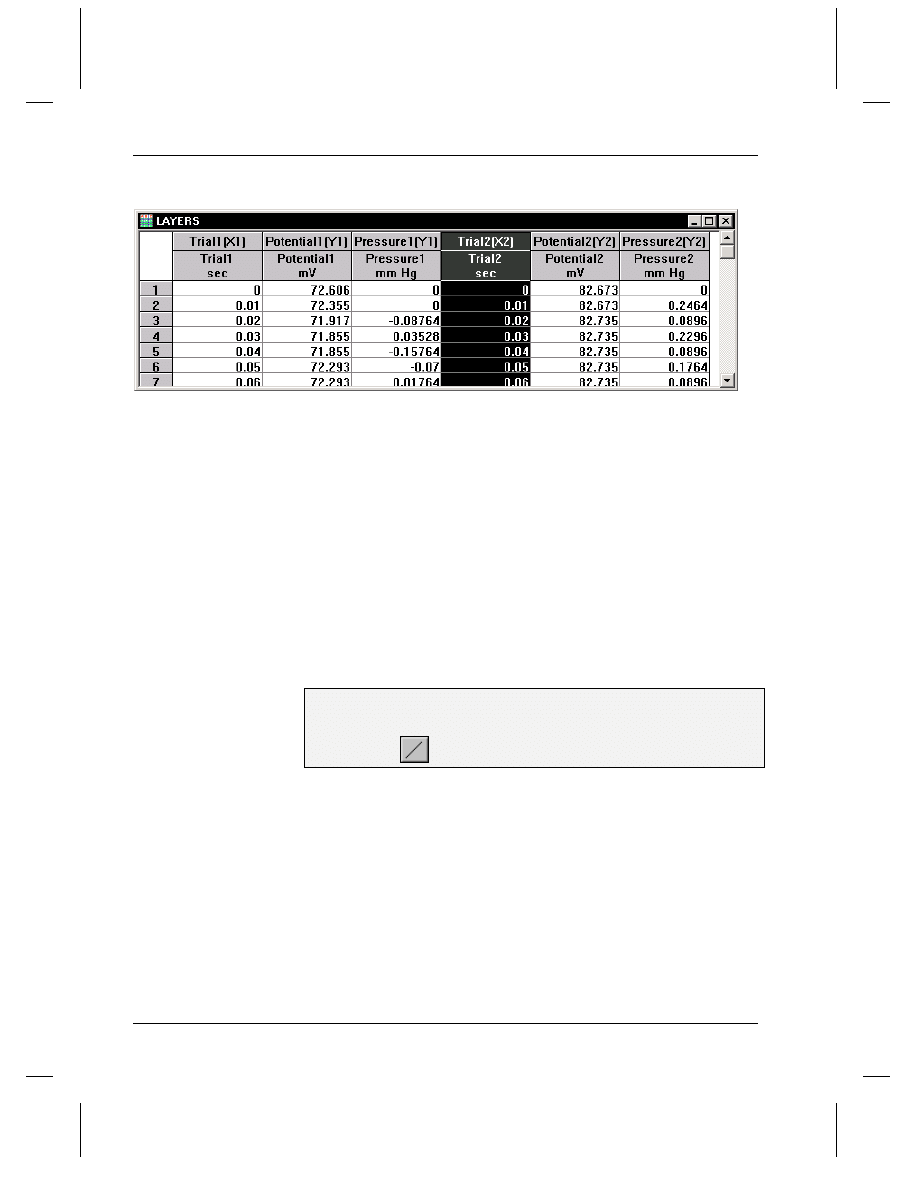
Tutorial 3, Creating Multiple Layer Graphs

128

•

Creating a Multiple Layer Graph

Figure 10: Setting Trial2 as X

Creating a Multiple Layer Graph

Origin does not contain pre-defined templates for all the different ways in
which layers can be arranged. However, you can create your own
custom multiple layer graph and save it as a template for future use.
The following steps describe a method for creating a multiple layer
graph, using a single layer graph as a starting point. This information is
provided to familiarize you with important layer concepts. However,
keep in mind that Origin provides a number of multiple layer graph
templates that you can use as a starting point for your custom multiple
layer graph.

To Create a Multiple Layer Graph:
1) Click on the Potential1 column heading to highlight the column.

2) Click Line

on the 2D Graphs toolbar.

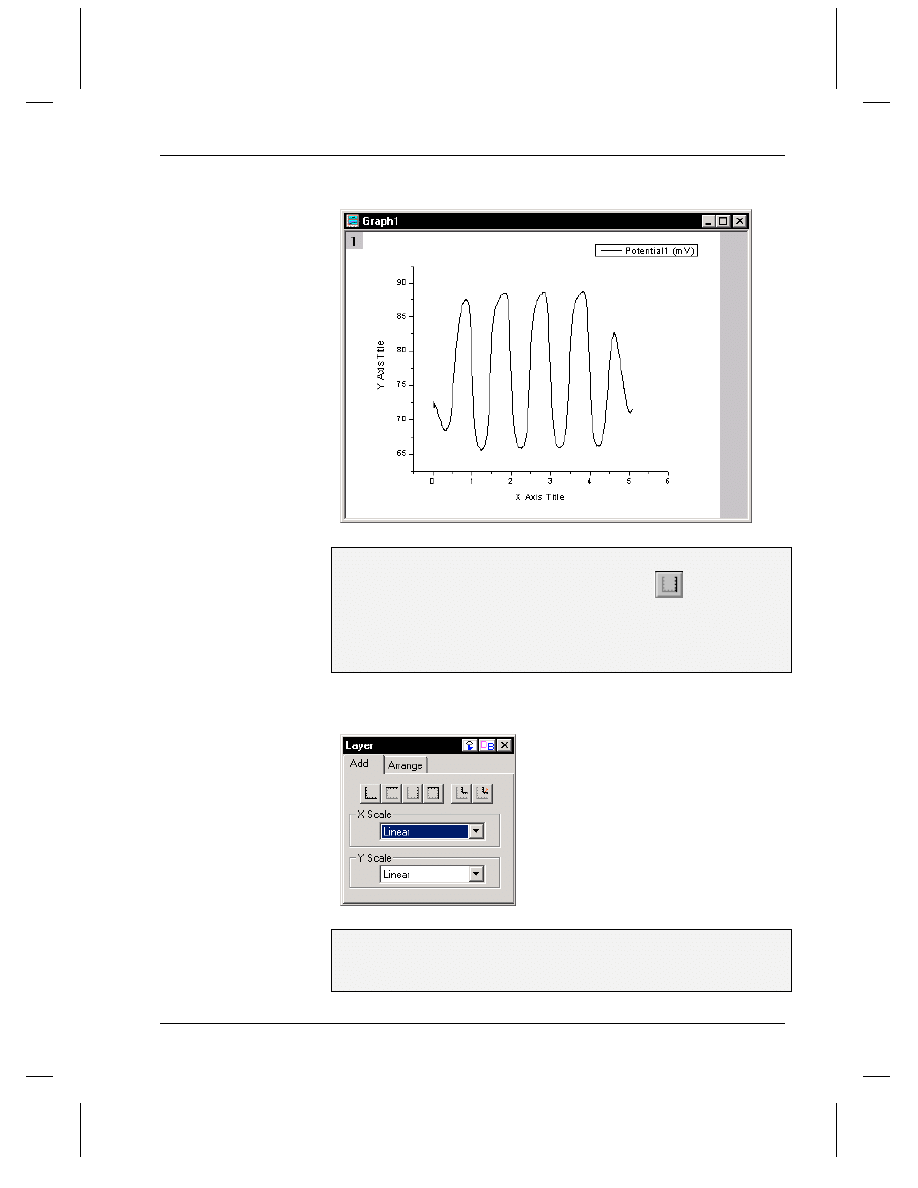
Tutorial 3, Creating Multiple Layer Graphs

Creating a Multiple Layer Graph

•

129

Figure 11: Line Graph of Potential1 Column

3) Select Tools:Layer to open the Layer tool.

4) With the Add tab selected, click Linked Right Y

. This adds a

second layer to the graph displaying only the right Y axis. By default,
the X axis of this layer is linked to the X axis of layer 1. This means that
if you change the X axis scale in layer 1, the X axis scale in layer 2
automatically updates with the change.

Figure 12: The Layer Tool

5) Double-click on the layer 2 icon in the upper-left corner of the graph
window.
6) Select layers_pressure1 in the Available Data list box.

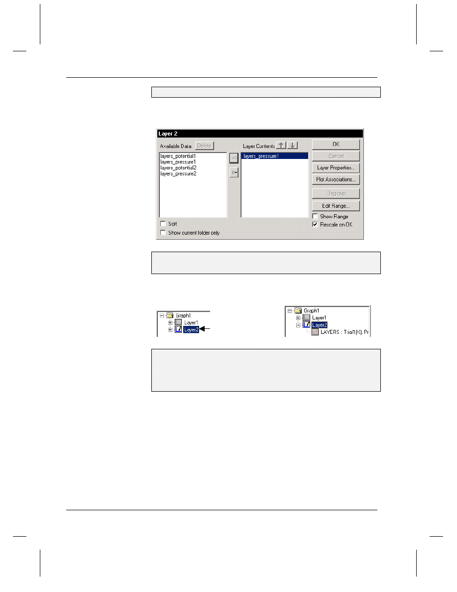
Tutorial 3, Creating Multiple Layer Graphs

130

•

Creating a Multiple Layer Graph

7) Click => to add the data set to the Layer Contents list box.

Figure 13: Adding Data to Layer 2

8) Click Layer Properties. The Plot Details dialog box opens.
9) Double-click on the Layer2 icon on the left side of the dialog box.

Figure 14: Opening the Layer Tree

Double-click here.

10) Click on the LAYERS:Trial1(X), Pressure1(Y) data plot icon on the
left side of the dialog box. This action opens the Line tab.
11) Select Blue from the Color drop-down list, then click OK.
12) Click OK to close the Layer 2 dialog box.

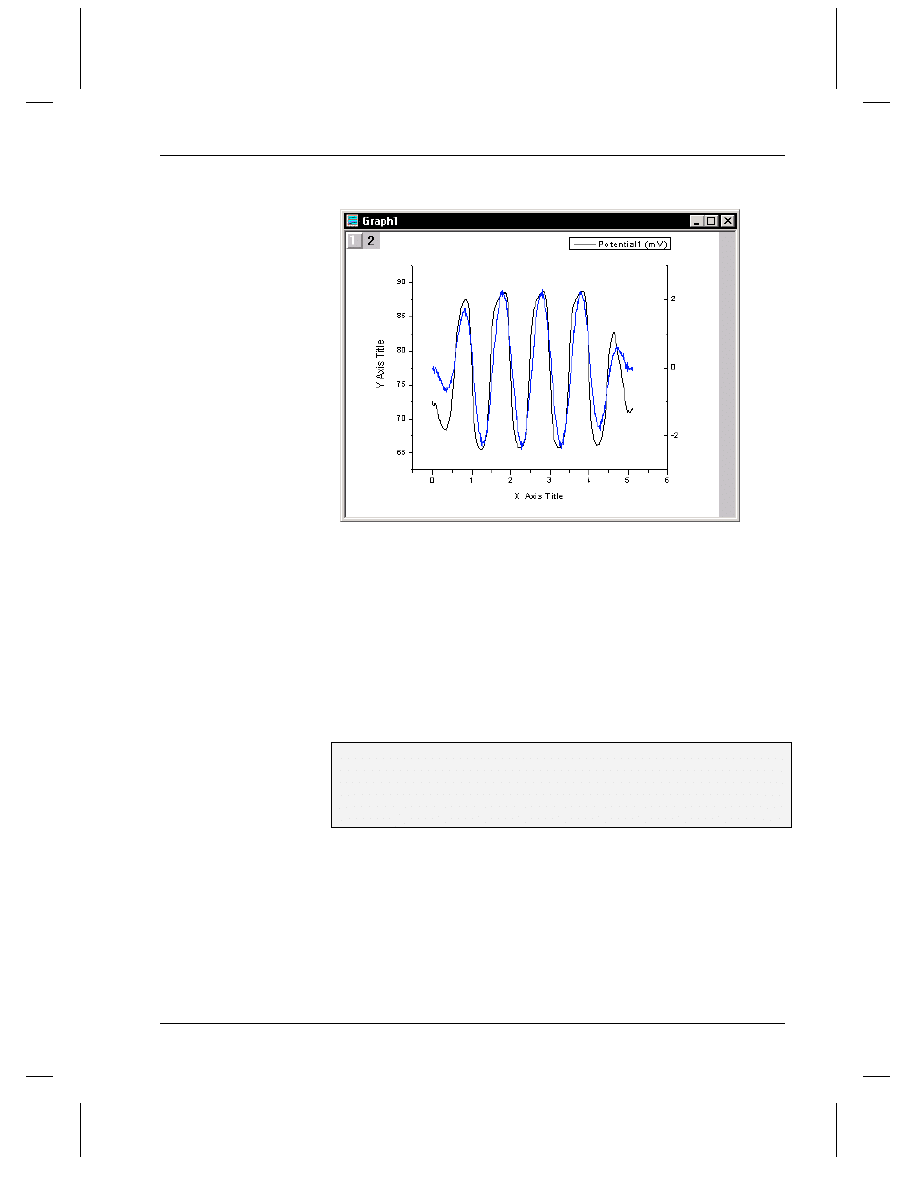
Tutorial 3, Creating Multiple Layer Graphs

Creating a Multiple Layer Graph

•

131

Figure 15: Adding a Right Y Controlling Axis and Data

Origin provides many methods to add layers to your graph. In addition
to the Layer tool, you can select menu commands from the Edit menu or
from a shortcut menu available outside of the graph page (but within the
window).

Arranging Layers in the Graph Window

In this section, you will add and arrange layers to set up a vertical 2 panel
graph with left and right Y axes.

To Add and Arrange Layers in the Graph:
1) Select Edit:Add & Arrange Layers.
2) In the Total Number of Layers dialog box, type 2 in the Number of
Rows text box.

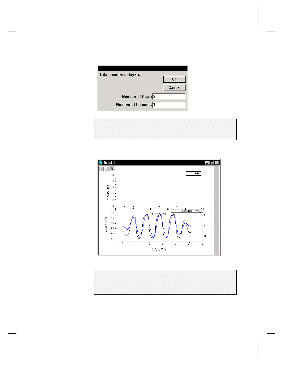
Tutorial 3, Creating Multiple Layer Graphs

132

•

Creating a Multiple Layer Graph

Figure 16: Setting the Number of Layers

3) Click OK. Origin asks for permission to create 1 more layer.
4) Click Yes.
5) Click OK in the Spacing dialog box to accept the default settings.

Figure 17: Adding and Arranging Layers

To Add the Right Y Controlling Axis to the Top Layer:
1) With the layer 3 icon selected, right-click in the gray area of the graph
window, outside of the page and select New Layer (Axes):(Linked):
Right Y from the shortcut menu.

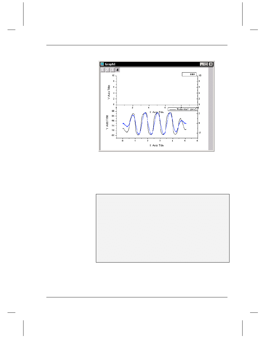
Tutorial 3, Creating Multiple Layer Graphs

Creating a Multiple Layer Graph

•

133

Figure 18: Adding a Right Y Axis to the Top Layer

Adding Data to the New Layers

To add the data to layers 3 and 4, you will use the Layer n dialog box in
the same way you added the data to layer 2.

To Add Data to the New Layers:
1) Double-click on the layer 3 icon.
2) In the Layer 3 dialog box, select layers_potential2 in the Available
Data list box, then click => to add it to the Layer Contents list box.
3) Click OK.
4) Double-click on the layer 4 icon.
5) In the Layer 4 dialog box, select layers_pressure2 in the Available
Data list box, then click => to add it to the Layer Contents list box.
6) Click Layer Properties to open the Plot Details dialog box.
7) Double-click on the Layer4 icon on the left side of the dialog box,
then click on the LAYERS:Trial2(X), Pressure2(Y) data plot icon.

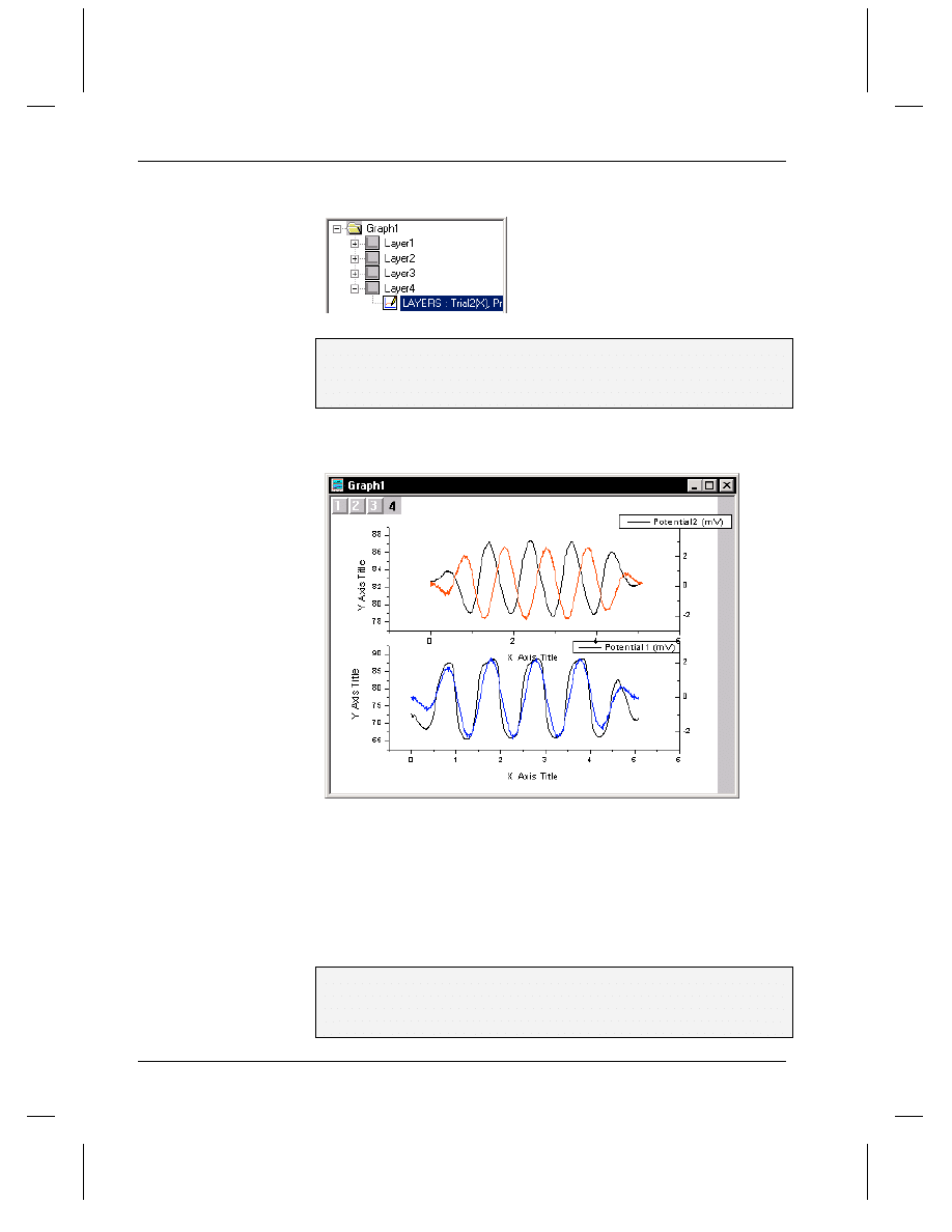
Tutorial 3, Creating Multiple Layer Graphs

134

•

Creating a Multiple Layer Graph

Figure 19: Graph Tree of Plot Details Dialog Box

8) Select Red from the Color drop-down list.
9) Click OK to exit the Plot Details dialog box.
10) Click OK in the Layer 4 dialog box.

Figure 20: Adding Additional Layers and Data

Linking Axes

You can link axes between layers so that when you change the axis scale
in one layer the other layer's linked axis updates to the same scale
automatically.

To Link the X Axes:
1) Double-click on the layer 3 icon to open the Layer 3 dialog box.
2) Click Layer Properties.

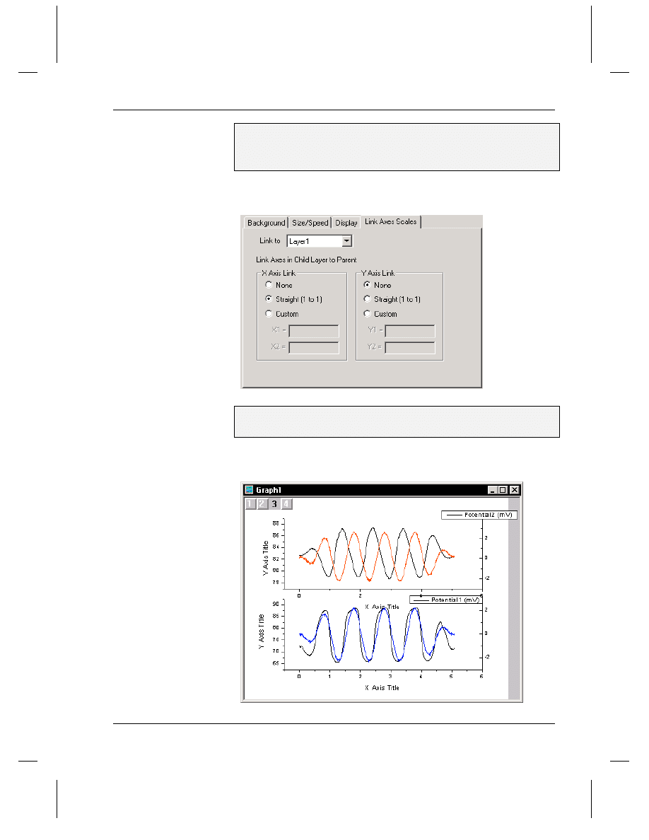
Tutorial 3, Creating Multiple Layer Graphs

Creating a Multiple Layer Graph

•

135

3) Select the Link Axes Scales tab.
4) Select Layer 1 from the Link To drop-down list.
5) Select the Straight (1 to 1) radio button in the X Axis Link group.

Figure 21: Setting the Axis Linking Relationship

6) Click OK to close the Plot Details dialog box.
7) Click OK in the Layer 3 dialog box.

Figure 22: Adding Data to the Layers

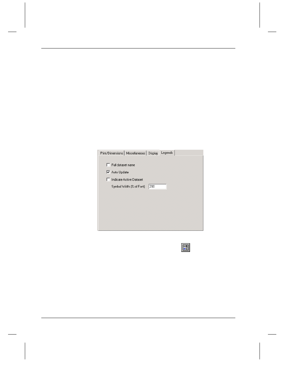
Tutorial 3, Creating Multiple Layer Graphs

136

•

Customizing the Legend

You can test the axis link by double-clicking on the bottom X axis and
changing the From or To values on the Scale tab. After clicking OK, the
top X axis also reflects your changes.

Customizing the Legend

Origin automatically displays a legend when you create a new graph.
Furthermore, legends are layer-specific, so that if your graph has multiple
layers, Origin displays a legend for each layer. If you add additional data
to a layer, the legend will not update to include the new data unless you
have selected the Auto Update check box on the Legends tab of the
page's Plot Details dialog box (Format:Page).

Figure 23: Setting the Legend to Update Automatically

You can also instruct Origin to update the legend for the active layer at

any time by clicking the New Legend button

on the Graph toolbar.

If there is currently no legend in the layer, Origin creates one.
A legend is a unique text label. Origin names the text label "Legend" to
identify it. This name is stored in the legend's Label Control dialog box.
You can open this dialog box by selecting the legend and then selecting
Format:Label Control. If you rename the legend, it will maintain its
current contents but it will no longer update when you click New Legend
or when you add data to the layer.

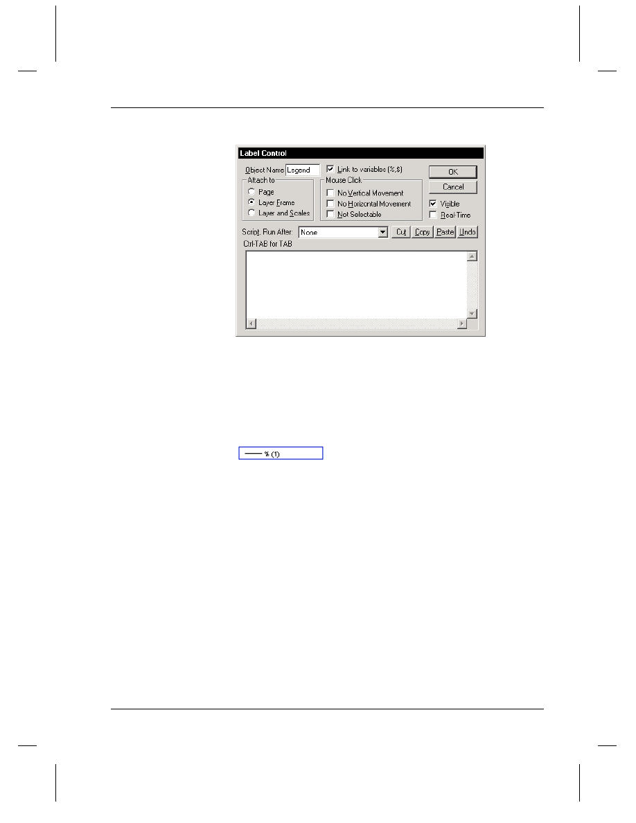
Tutorial 3, Creating Multiple Layer Graphs

Customizing the Legend

•

137

Figure 24: The Label Control Dialog Box for a Legend

A legend text label also uses special formatting to display the data set
names and the data plot type icon (such as a line). If you double-click on
the legend in the top layer of the current example, the in-place editing
mode will display as shown in the following figure.

Figure 25: In-place Editing of a Legend Text Label

The %(1) is called substitution notation. This notation instructs Origin to
display the data set name for the first data set in this layer.
When you are in-place editing any label, you can use substitution
notation. For example, you can display the value of a specific data point
in a data plot using the following substitution notation:
%(WorksheetName, ColumnNumber, RowNumber)
For example, if a worksheet is named data1, and you have plotted
columns A(X) and B(Y), you can display the value of the data point in
column 2, row 3 using:
%(data1, 2, 3)
To use this substitution notation, you must select the Link to Variables
(%,$) check box in the Label Control dialog box (Figure 24).
In addition to substitution notation, Origin uses a special escape sequence
to display the data plot icon in the legend (such as a line). This special
escape sequence is:
\L(DataListPosition)
Where DataListPosition is the data plot's position in the data list, the list

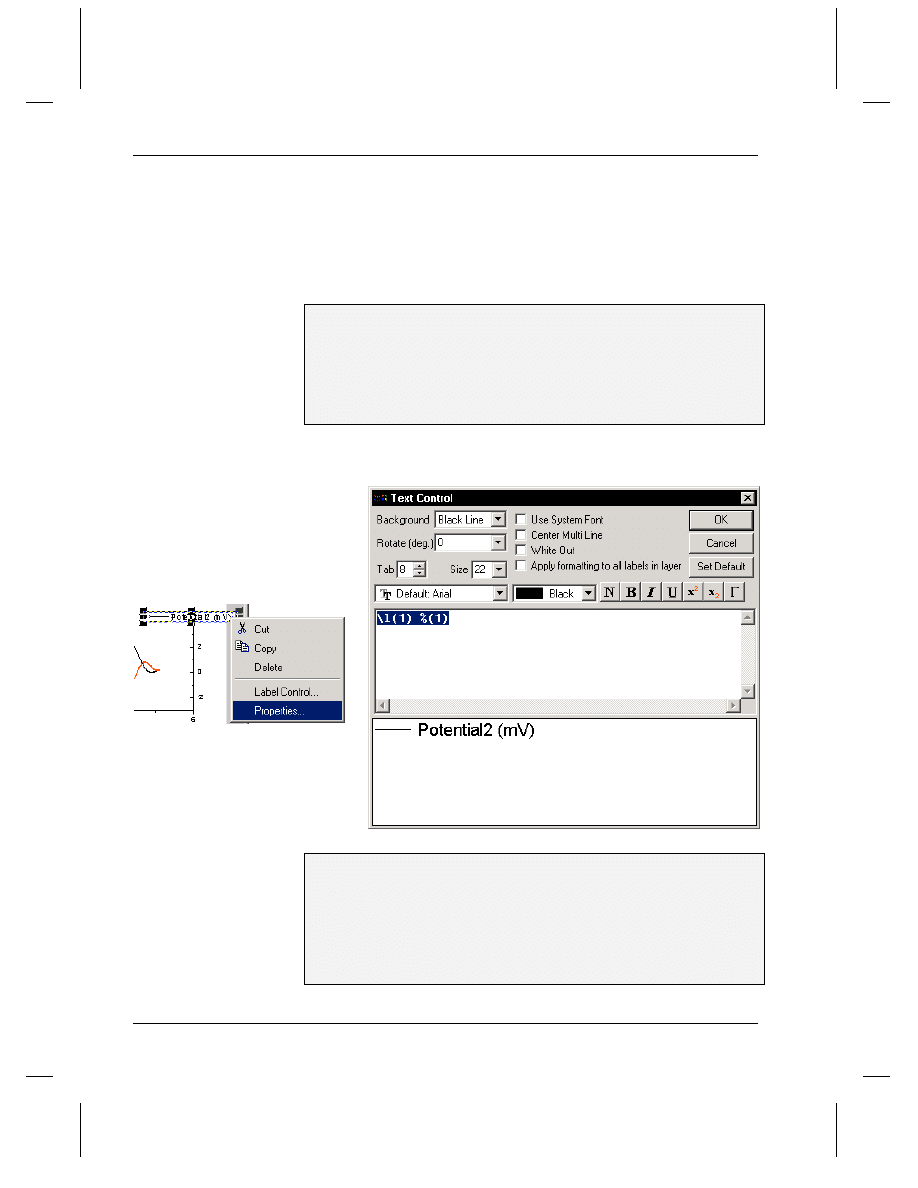
Tutorial 3, Creating Multiple Layer Graphs

138

•

Customizing the Legend

of plotted data at the bottom of the Data menu.
If you double-click on a legend to enter the in-place editing mode, you
will see the data plot icon, not the \L( ) escape sequence. This is because
Origin does not support using escape sequences in the in-place editing
mode. To use escape sequences, you must edit the label in the Text
Control dialog box (see the following instructions).

To Customize the Legend:
1) In the bottom layer, click on the text portion of the legend reading
Potential1 (mV), then press DELETE.
2) In the top layer, right-click on the text portion of the legend reading
Potential2 (mV) and select Properties from the shortcut menu. This
opens the Text Control dialog box.

Figure 26: Opening the Text Control Dialog Box

3) In the Text Control dialog box, type the following text, overwriting
\L(1) %(1):
\L(1.1) Potential1
\L(2.1) Pressure1
\L(3.1) Potential2
\L(4.1) Pressure2

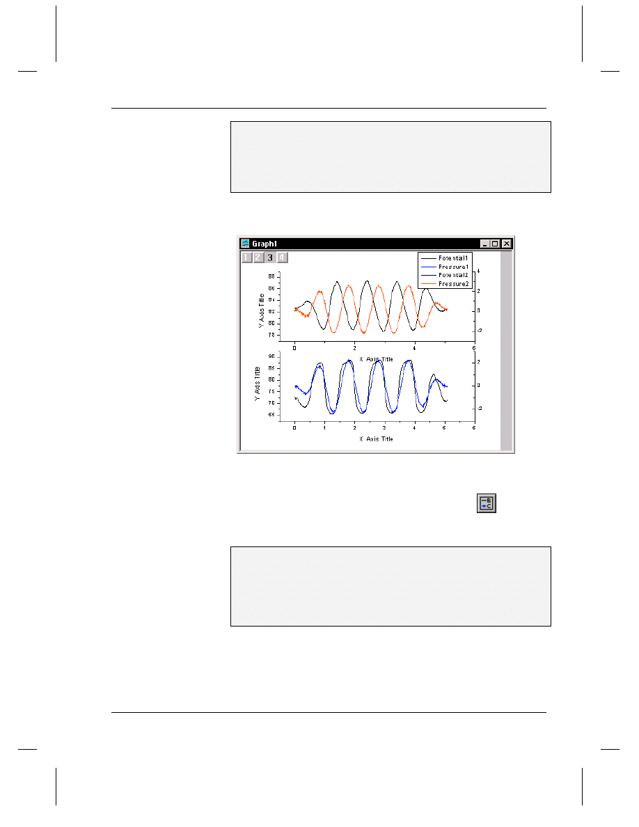
Tutorial 3, Creating Multiple Layer Graphs

Customizing the Legend

•

139

The preview box on the bottom of the dialog box shows what the text
will look like in the legend.
4) Click OK.
5) If necessary, drag the legend to a new location to minimize
overlapping of graphic elements.

Figure 27: Updating the Legend to Include All the Data

The legend now displays the data plot type representations from all the
layers in the graph. To prevent Origin from overwriting your custom

legend (for example, if you click the New Legend button

on the

Graph toolbar) you can rename the legend.

To Rename the Legend:
1) Right-click on the legend text.
2) Select Label Control from the shortcut menu that opens.
3) Type Custom Legend in the Object Name text box.
4) Click OK.

Tutorial 3, Creating Multiple Layer Graphs

140

•

Saving the Graph as a Template

Template files retain information on how to display the data, but do not
actually save the data. If you save the current graph window as a
template, then the next time you need to create a similar graph, you can
select your worksheet data and then select your custom graph template.
Your custom template is easily accessed by clicking the Template button

on the 2D Graphs toolbar or by selecting Plot:Template Library.

To Save Your Graph as a Template:
1) Right-click on the graph window title bar.
2) Select Save Template As from the shortcut menu.
3) Type Multilayer in the File Name text box.
4) Type My Templates in the Template Category combo box.
5) Click Save.

To test your template, you can make the Layers worksheet active, select
all the worksheet columns, and then select Plot:Template Library.
Select the My Templates category and then select your Multilayer
template. Click Plot to plot your data.

Tutorial 4, Nonlinear Curve Fitting

Introduction

•

141

Tutorial 4, Nonlinear Curve

Fitting

Introduction

Origin offers several methods of fitting functions to your data. These
methods vary in speed and complexity to optimize fitting for all users. In
this tutorial, you will be introduced to fitting using the menu commands,
the tools, the fitting wizard (NLSF Wizard), and the advanced fitting tool
(NLSF). You will then use the NLSF to define your own function and fit
sample data.
In addition to defining functions in the NLSF, Origin provides a C
programming language called Origin C and an integrated development
environment called Code Builder for defining and compiling functions.
Once compiled, you can access the function from the NLSF. To learn
more:
=> Review the AsymGauss.OPJ project that is located in the Origin
\Samples\Programming\NLSF User-defined Function folder.
=> Review "Tutorial 8, Programming in Origin".

Fitting from the Menu

Origin offers access to several fitting functions directly from the
Analysis menu. To perform a fit on your data using the menu
commands, make sure that the data plot you want to perform the fit on is
active, then select the type of fit you want to perform from the Analysis
menu. Most of the menu commands require no parameter information
from you and will carry out the fit automatically. Some may ask you for
some parameter information, but will suggest default values based on
your data.

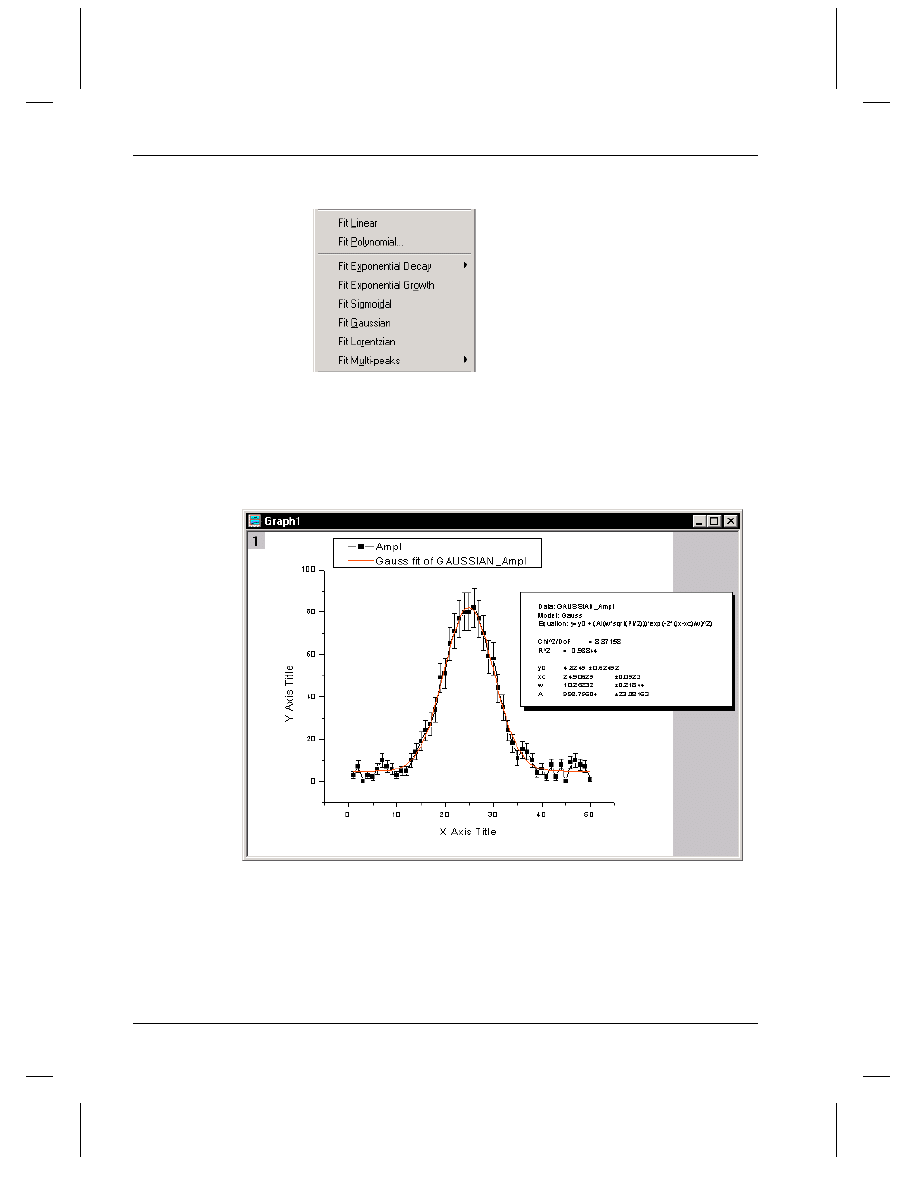
Tutorial 4, Nonlinear Curve Fitting

142

•

Fitting from the Menu

Figure 1: Fitting Commands from the Graph Window Analysis Menu

After performing the fit, Origin displays the fit curve and results
(depending on the fit selection) in the graph window, and outputs the full
results to the Results Log.

Figure 2: Fitting from the Analysis Menu

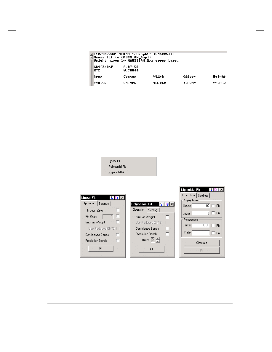
Tutorial 4, Nonlinear Curve Fitting

Fitting Using the Tools

•

143

Fitting Using the Tools

For a greater degree of control than the menu commands allow, Origin
provides three fitting tools: the Linear Fit, Polynomial Fit, and
Sigmoidal Fit tools. These tools are available from the Tools menu when
a worksheet or a graph is active.

Figure 3: The Fitting Tools

To use the fitting tools, select the data set or data plot you want to fit,
open the tool and customize the options on both tabs of the tool, and then
click Fit on the Operation tab.

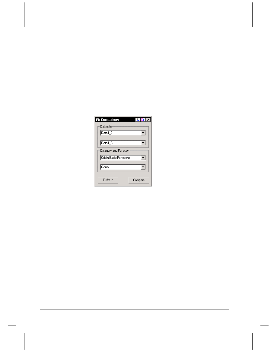
Tutorial 4, Nonlinear Curve Fitting

144

•

Fitting Comparison

A Fit Comparison tool is available to determine if two data sets are
representative samples from the same population or not. This tool
compares the data sets by fitting the same function to the data. It then
uses an F-test to determine whether the data sets are significantly
different from each other. To open the Fit Comparison tool when a
worksheet or graph is active, select Tools:Fit Comparison.

Figure 4: The Fit Comparison Tool

This tool outputs the results to the Results Log.

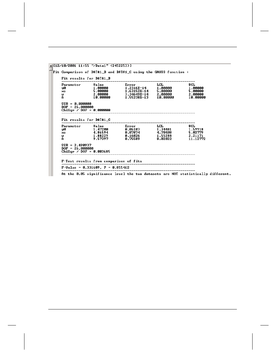
Tutorial 4, Nonlinear Curve Fitting

The Fitting Wizard

•

145

Figure 5: The Fit Comparison Results

The Fitting Wizard

Origin provides both a wizard (NLSF Wizard) and an advanced fitting
tool (NLSF) for performing nonlinear least squares fitting. The wizard
steps you through the fitting process, and is thus easier to use than the
NLSF. However, the wizard does not provide all the fitting options
available in the NLSF. For example, if you want to define a new fitting
function, fit multiple data sets to a function, fit with multiple independent
or dependent variables, or run scripts at specified triggers (for example,
after a fit is performed), then you must use the NLSF.
To open the NLSF Wizard when a worksheet or graph is active, select
Analysis:Nonlinear Curve Fit:Fitting Wizard.

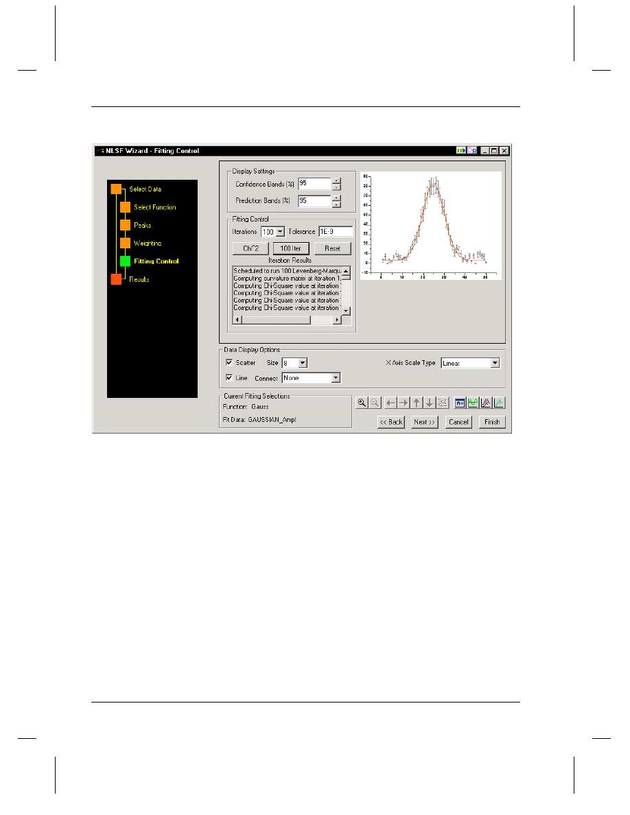
Tutorial 4, Nonlinear Curve Fitting

146

•

The Advanced Fitting Tool

Figure 6: The NLSF Wizard (Fitting Control Page)

The Advanced Fitting Tool

The advanced fitting tool (NLSF) is Origin's most powerful and complex
method of fitting data. To open the NLSF when a worksheet or graph is
active, select Analysis:Nonlinear Curve Fit:Advanced Fitting Tool.
There are two display modes available for the NLSF: basic and
advanced. You can switch between modes by clicking the More button
in the basic mode or the Basic Mode button in the advanced mode.

The Basic Mode

The basic mode of the NLSF provides an abbreviated fitting function list
and a less complex interface than the advanced mode. Additionally, the
basic mode offers less control over the fit and less customization of the
reported results.

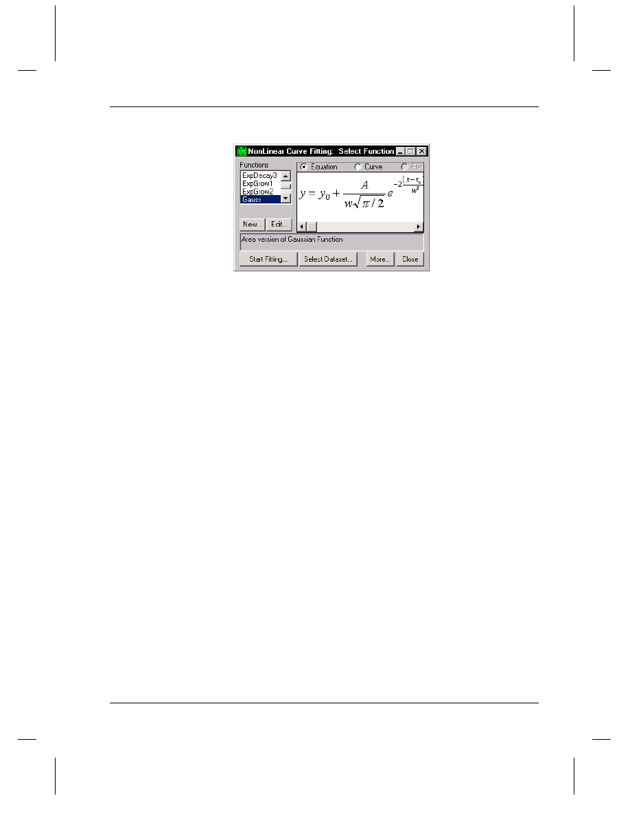
Tutorial 4, Nonlinear Curve Fitting

The Advanced Fitting Tool

•

147

Figure 7: Basic Mode of the NLSF

The Advanced Mode

The advanced mode lets you customize all aspects of the fitting process.
It provides access to many more fitting functions than the basic mode and
the functions are separated into categories to facilitate searching. The
advanced mode also has its own menu and toolbar to provide access to all
its features.
To select a function in the advanced mode, first select Function:Select
from the NLSF menu if the Select Function page is not active. Then
select the appropriate category from the Categories list box, and select
the desired function from the Functions list box. Once a function is
selected, the procedure for fitting is the same as for fitting after you
define your own function (see the following sections).

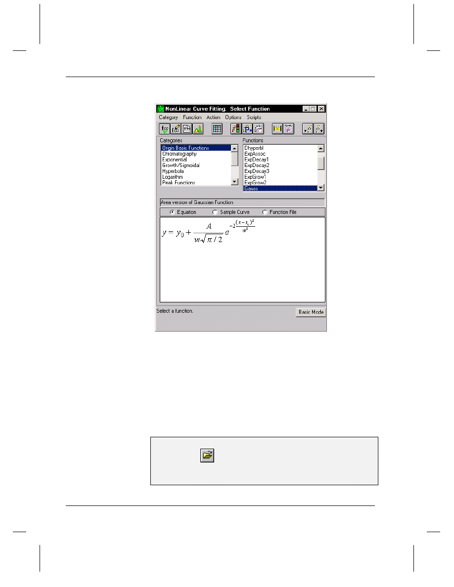
Tutorial 4, Nonlinear Curve Fitting

148

•

Fitting a Data Set Using Your Own Function

Figure 8: Advanced Mode of the NLSF

Fitting a Data Set Using Your Own Function

Opening the Project File

The data for this tutorial is provided in an Origin project file.

To Open the Project File:

1) Click Open

on the Standard toolbar.

2) In the Origin \TUTORIAL folder, select TUTORIAL_4.OPJ from the
list of files.

Tutorial 4, Nonlinear Curve Fitting

Fitting a Data Set Using Your Own Function

•

149

3) Click Open.

The project opens showing a worksheet containing data and a graph
window containing a data plot.

Defining a Function

You can define your own function in the NLSF and then access that
function in future sessions. In the basic mode, you click New to define a
function. The following procedure guides you through defining a
function in the advanced mode.

To Define your own Function in the Advanced Mode:
1) Select Analysis:Nonlinear Curve Fit:Advanced Fitting Tool. This
opens the NLSF.
2) If the NLSF opens in the basic mode, click More to switch to the
advanced mode. (See pages 147 and 148 for pictures of the basic and
advanced modes.)
3) Select Function:New from the NLSF menu bar. This activates the
Define New Function dialog box.
4) Type MyFitFunc in the Name text box.
5) Select 3 from the Number of Parameters drop-down list.
6) Type p1*exp(-x^p2/p3) in the Definition text box.

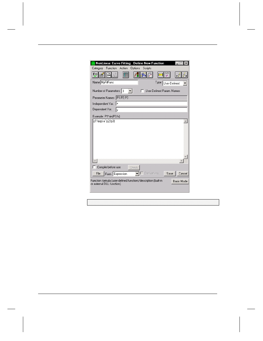
Tutorial 4, Nonlinear Curve Fitting

150

•

Fitting a Data Set Using Your Own Function

Figure 9: Defining a New Function

7) Click Save.

The function is saved under the name MyFitFunc. The MyFitFunc
function will now be available in the list of functions under the currently
active category. The currently active category is the selected category In
the NLSF Select Function dialog box (Function:Select from the NLSF
menu).

Assigning the Function Variables to the
Data Sets

The next step is to assign the X and Y variables in the function to the
corresponding X and Y data sets in the data plot you are fitting.

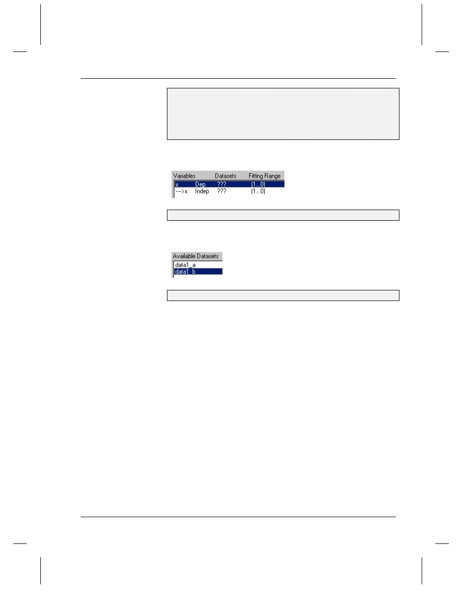
Tutorial 4, Nonlinear Curve Fitting

Fitting a Data Set Using Your Own Function

•

151

To Assign the Function Variables to Data Sets:
1) Select Action:Dataset from the NLSF menu bar. This activates the
Select Dataset dialog box.
2) In the list box at the top of the fitter, the Y variable should be selected
in the list. If not, select it.

Figure 10: Selecting the Y Variable

3) In the Available Datasets list box, select data1_b.

Figure 11: Selecting the Data Set

4) Click Assign.

When you assign the Y variable to data1_b (the Y data set), Origin
automatically assigns the X variable to data1_a (the associated X data
set).

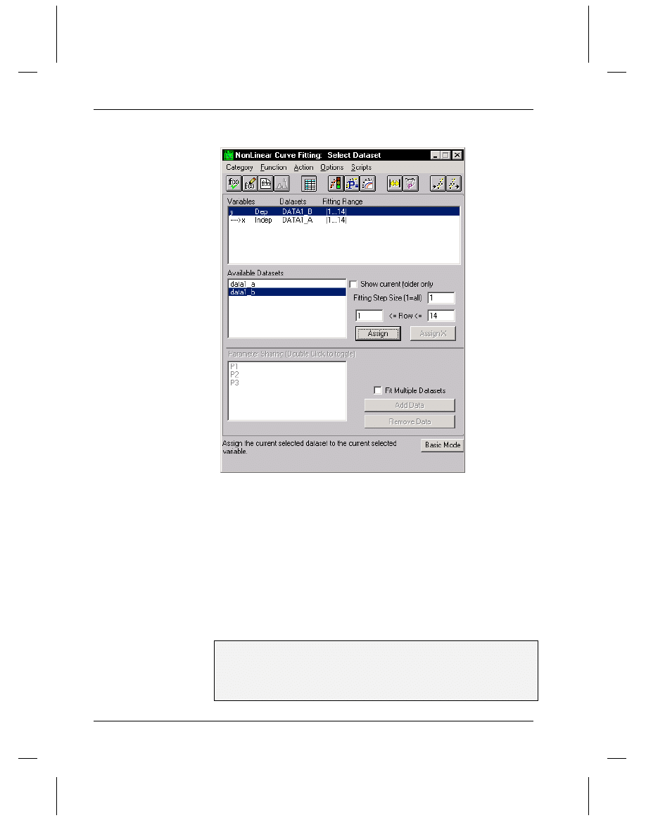
Tutorial 4, Nonlinear Curve Fitting

152

•

Fitting a Data Set Using Your Own Function

Figure 12: Assigning Variables to Data Sets

Simulating Curves to Initialize the
Parameter Values

Origin lets you observe what the function will look like with various
parameter values in the Simulate Curves dialog box. This enables you to
get an understanding of which parameter values produce curves that look
similar to your data. This is important because reasonably good starting
parameter values are in most cases a precondition for the success of the
fitting process.

To Simulate Curves:
1) Select Action:Simulate from the NLSF menu bar. This activates the
Simulate Curves dialog box.
2) Type 5 in the P1, P2, and P3 text boxes (overwriting the dashes).

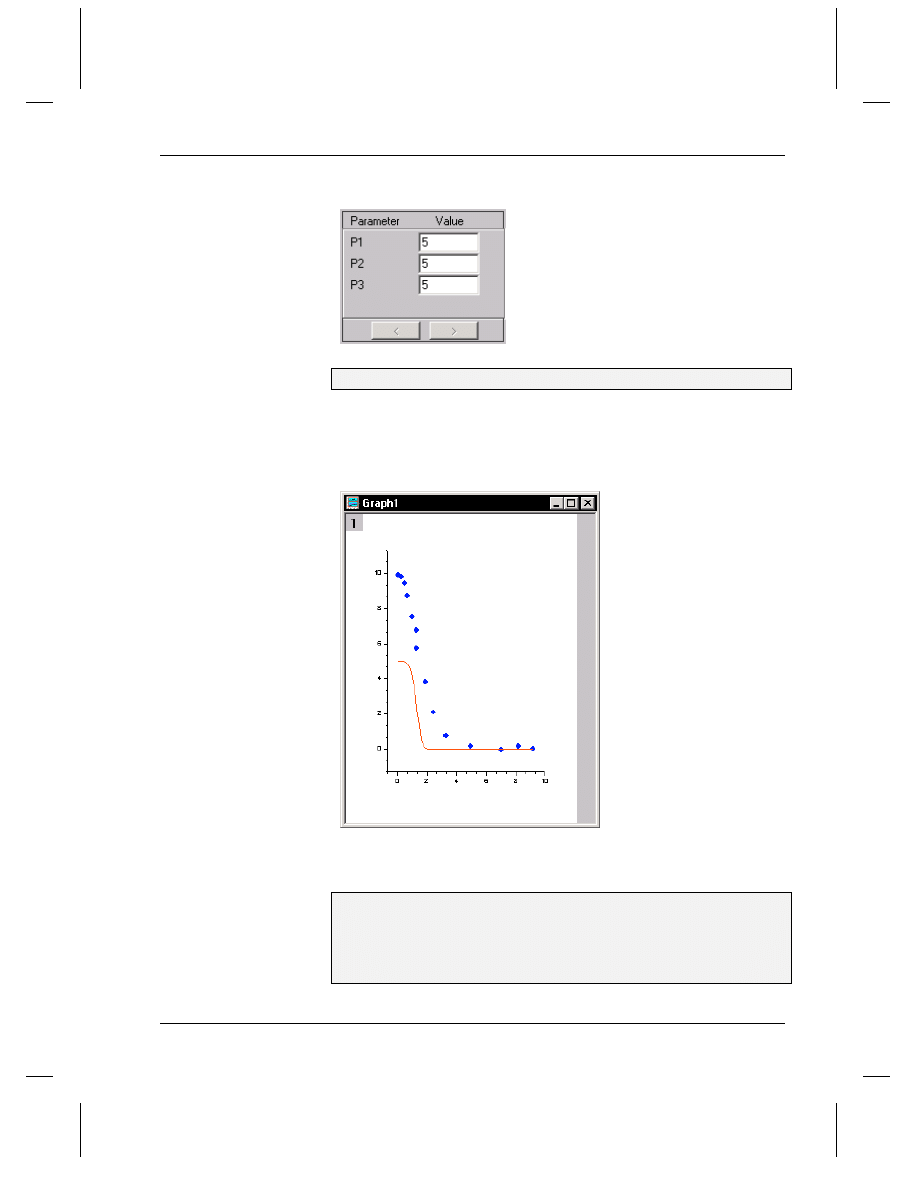
Tutorial 4, Nonlinear Curve Fitting

Fitting a Data Set Using Your Own Function

•

153

Figure 13: Initializing Parameter Values

3) Click Create Curve.

The parameters you typed in the text boxes are used to create a curve
which is plotted in the graph window containing your data plot.

Figure 14: Simulated Curve

You can type new parameter values in the text boxes to create a
simulated curve which looks more like your data.

4) Type 10 in the P1 text box (overwriting 5).
5) Click Create Curve.
6) Type 1 in the P2 and P3 text boxes (overwriting 5).
7) Click Create Curve.

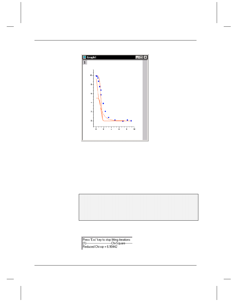
Tutorial 4, Nonlinear Curve Fitting

154

•

Fitting a Data Set Using Your Own Function

Figure 15: Fine-tuning the Simulated Curve

The simulated curve is much more similar to the plotted data with the last
set of parameter values. These will be the initial parameter values when
Origin fits the data.

Fitting the Data

You will now fit the data using the function you defined. The initial
parameter values will be used from the Simulate Curves dialog box.

To Fit the Data:
1) Select Action:Fit from the NLSF menu bar. This activates the Fitting
Session dialog box.
2) Click Chi-Sqr. The reduced chi-squared value for the current
parameter values displays in the view box.

Figure 16: Calculating the Reduced Chi-Square Value

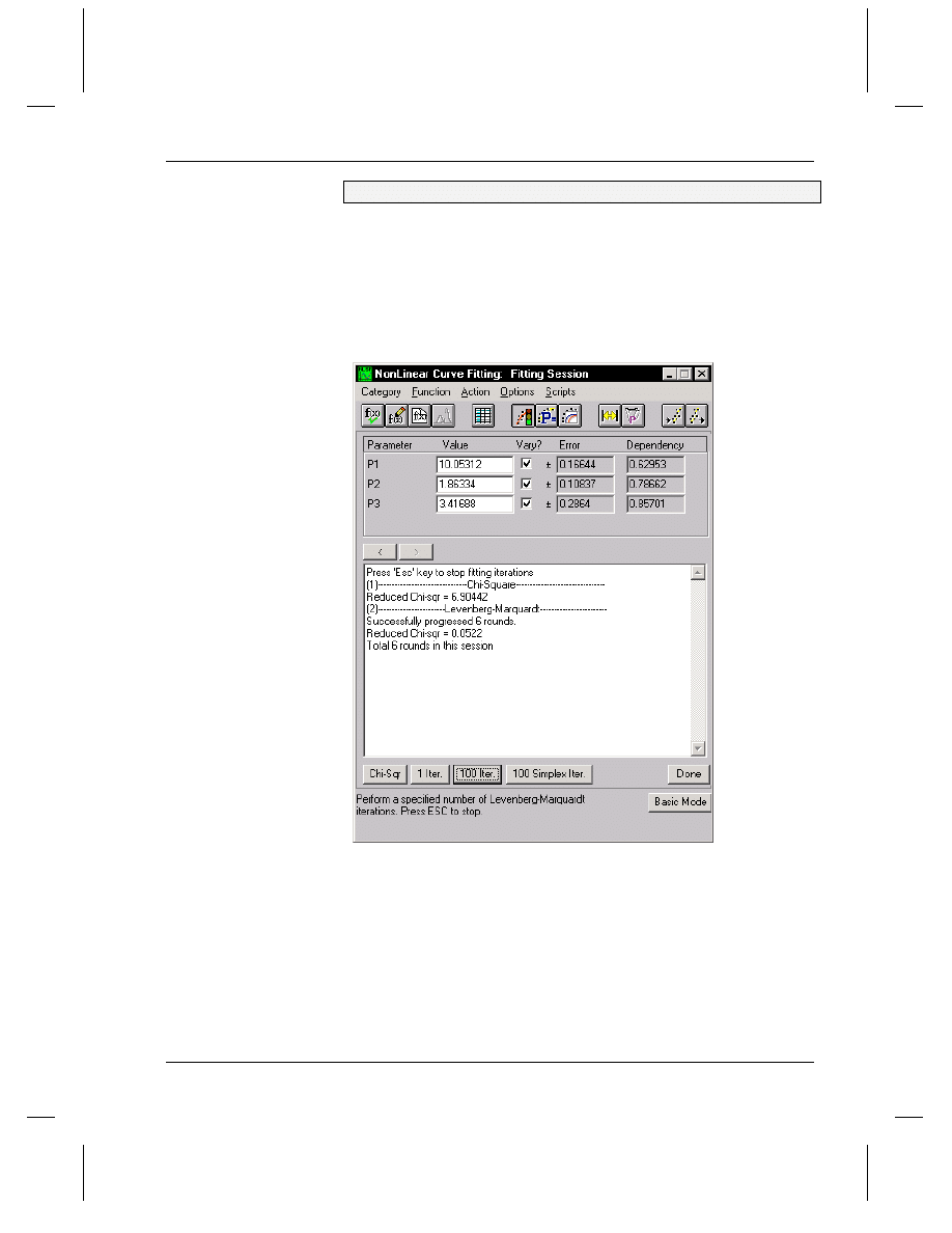
Tutorial 4, Nonlinear Curve Fitting

Fitting a Data Set Using Your Own Function

•

155

3) Click 100 Iter.

Origin fits the data, performing a maximum of 100 Levenberg-Marquardt
iterations. The fit curve displays in the graph. The reduced chi-squared
value and the number of iterations performed are reported in the NLSF
view box. The updated parameter values are shown in the Value text
boxes.

Figure 17: Fitting Session

Creating a Worksheet With the Fitting
Results and Exiting the Fitter

After fitting your data, you can create a worksheet that contains all the
results of your fitting session. Additionally, when you close the NLSF,
Origin displays the parameter fitting results in the Results Log and in a
label in the graph window.

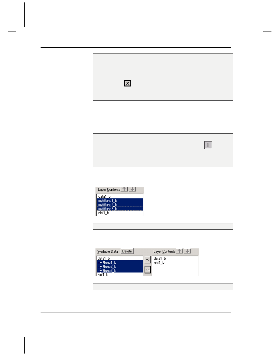
Tutorial 4, Nonlinear Curve Fitting

156

•

Fitting a Data Set Using Your Own Function

To Create a Worksheet with the Fitting Results:
1) Select Action:Results in the NLSF. This activates the Generate
Results dialog box.
2) Click Param. Worksheet.

3) Click Close

in the upper-right corner of the NLSF to close the

NLSF.
4) Click Yes at the Attention prompt.

After closing the NLSF, a Parameters worksheet displays all the fitting
results.
The graph window displays your data plot, the simulated curves, the fit
curve, and a text label with the parameter results.

To Remove the Simulated Curves from the Graph:

1) In the Graph1 window, double-click on the layer 1 icon

located

in the upper-left corner. This opens the Layer 1 dialog box.
2) Select the myfitfunc1_b, myfitfunc2_b, and myfitfunc3_b data sets
in the Layer Contents list box.

Figure 18: Selecting Data Sets in the Layer

3) Click <= to move the selected data sets out of the layer.

Figure 19: Moving the Data Sets Out of the Layer

4) Click OK to close the Layer 1 dialog box.

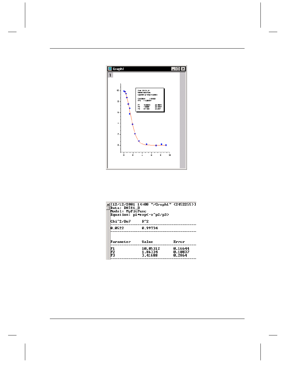
Tutorial 4, Nonlinear Curve Fitting

Fitting a Data Set Using Your Own Function

•

157

Figure 20: Final Graph

The Results Log also displays the parameter results.

Figure 21: The Fitting Results in the Results Log

Tutorial 4, Nonlinear Curve Fitting

158

•

Fitting a Data Set Using Your Own Function

Tutorial 5, Creating 3D Surface Graphs

Introduction to Matrices

•

159

Tutorial 5, Creating 3D Surface

Graphs

Introduction to Matrices

There are two primary data structures in Origin: worksheets and
matrices. Data stored in worksheets can be used to create any 2D graph
and some 3D graphs, but in order to create a 3D surface graph or a 3D
contour graph you must have your data stored in a matrix. Origin
provides methods for converting worksheets to matrices, and for
converting matrices to worksheets.
Matrices have numbered columns which are mapped to linearly spaced X
values and numbered rows which are mapped to linearly spaced Y
values. You can view the X and Y values in the matrix column and row
headings by selecting View:Show X/Y. Each cell value in a matrix
represents a Z value which is located in the XY plane by the cell's X
value (determined by its column) and by the cell's Y value (determined
by its row).

To Learn More about the XY Mapping in a Matrix:

1) Click the New Matrix button

on the Standard toolbar to create an

empty matrix.
2) Select Matrix:Set Dimensions to specify its dimensions and
coordinates.
3) In the Dimensions group, type 11 in the Columns text box and 21 in
the Rows text box.
4) In the Coordinates group, type -10 in both the First X text box and the
First Y text box.
5) In the Coordinates group, type 10 in both the Last X text box and the
Last Y text box.

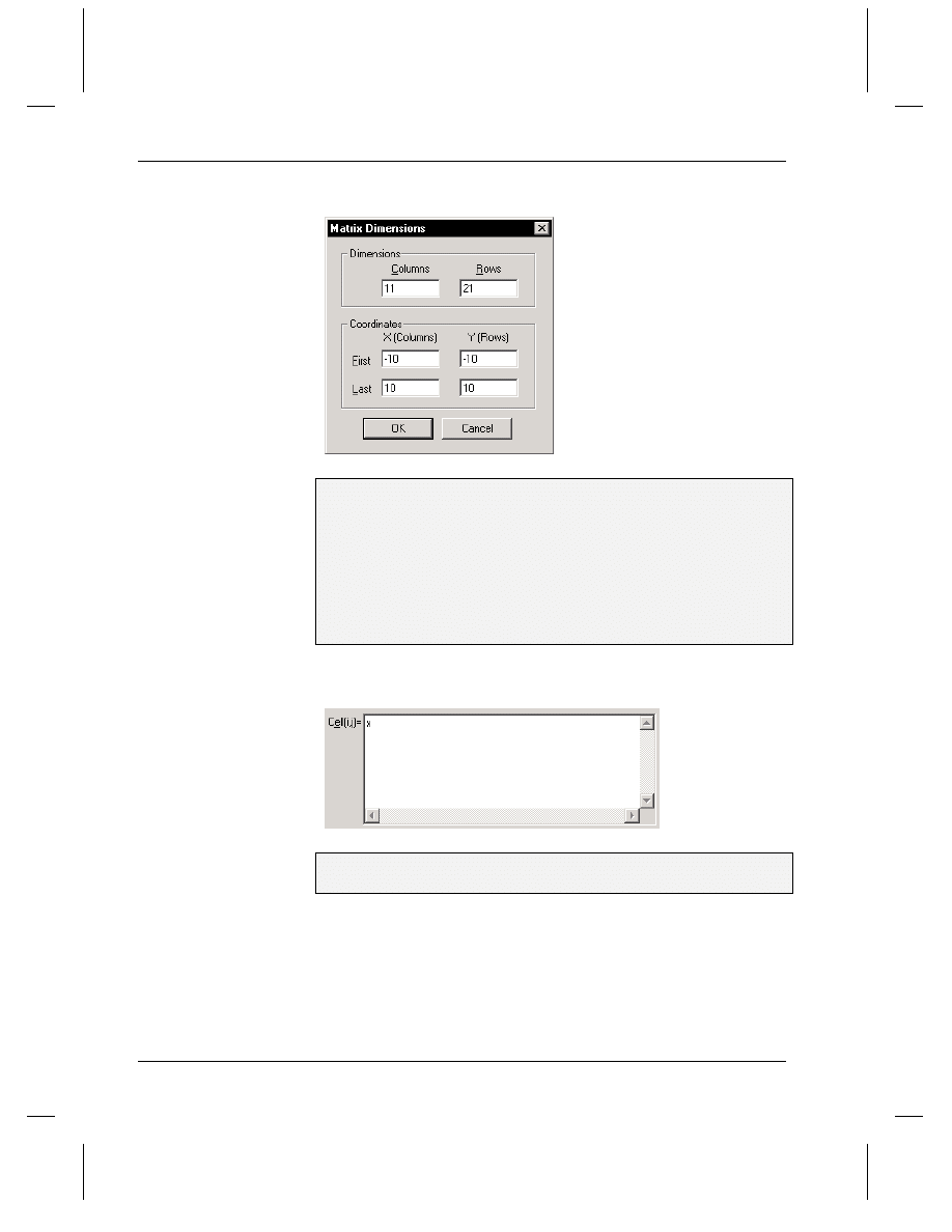
Tutorial 5, Creating 3D Surface Graphs

160

•

Introduction to Matrices

Figure 1: Setting the Matrix Dimensions and XY Coordinates

6) Click OK. You have created a matrix with 11 columns and 21 rows
with each dimension mapped to the coordinates from -10 to 10.
7) Select View:Show X/Y to view the X and Y values in the matrix
column and row headings.
8) Size and position the new matrix so that you can see all 11 columns
and all 21 rows.
9) Select Matrix:Set Values to fill the empty cells with Z values. As a
demonstration, type x in the Cell(i,j)= text box.

Figure 2: Setting the Matrix Z Values

9) Click OK. Each cell in each column is filled with a number equal to
the X value of its column.

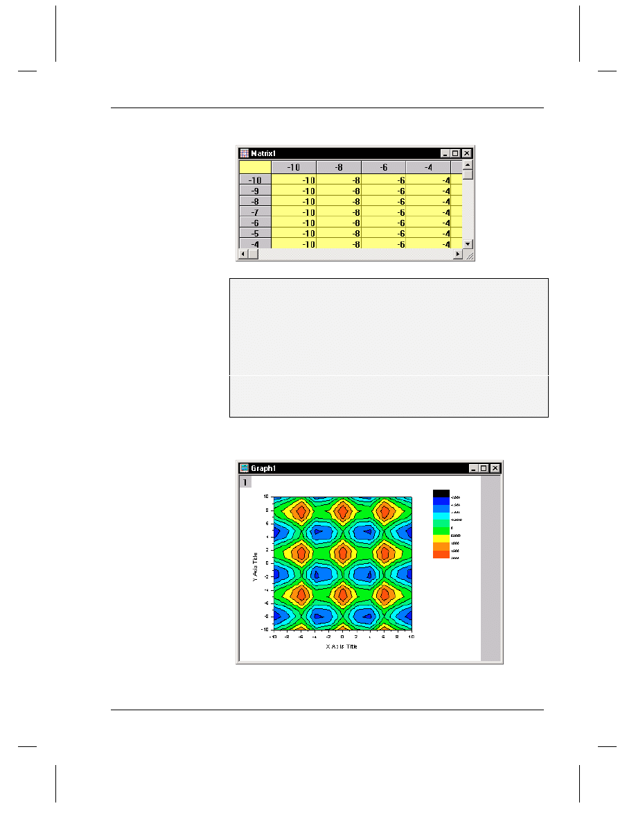
Tutorial 5, Creating 3D Surface Graphs

Introduction to Matrices

•

161

Figure 3: Filling Each Column with its X Value (full matrix not shown)

10) Re-select Matrix:Set Values and this time type y (replacing x) in
the Cell(i,j)= text box.
11) Click OK. Each cell in each row is filled with a number equal to the
Y value of its row.
12) Re-select Matrix:Set Values and type the equation cos(x)+sin(y) in
the Cell(i,j)= text box.
13) Click OK.
14) Select Plot:Contour Plot:Contour-Color Fill to create a contour
graph of the matrix data. Note the X and Y scales (-10 to 10) on the
resulting graph.

Figure 4: Creating a Contour Graph of the Matrix Data

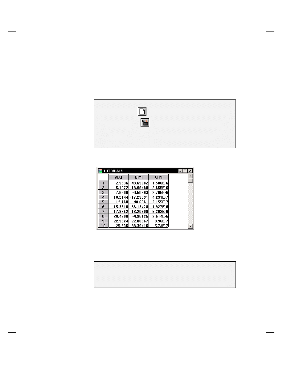
Tutorial 5, Creating 3D Surface Graphs

162

•

Converting a Worksheet to a Matrix

In this section you will learn how to change a worksheet column’s
designation, then convert an XYZ worksheet to a matrix so that it can be
plotted as a 3D surface graph.
The data for this lesson is provided in an ASCII file.

To Import the ASCII File:

1) Click New Project

on the Standard toolbar.

2) Click Import ASCII

on the Standard toolbar.

3) In the Origin \TUTORIAL folder, select TUTORIAL_5.DAT from
the list of files.
4) Click Open.

Figure 5: Importing the ASCII File

By default, when the file is imported columns are added to the worksheet
as Y columns. To convert the worksheet to a matrix it must be in an
XYZ format.

To Change the Column Designation:
1) Right-click on the C(Y) column heading.
2) Select Set As:Z from the shortcut menu. Column C is now
designated as a Z column.

Tutorial 5, Creating 3D Surface Graphs

Converting a Worksheet to a Matrix

•

163

Selecting the Type of Conversion

Origin provides several methods for converting worksheets to matrices,
including direct, expand columns, 2D binning, regular XYZ and random
XYZ conversions. The method that you use will depend on the type of
data in the worksheet.
=> Direct Conversion: A common format for XYZ worksheet data is
to have X data values in the left-most column, Y data values in the first
row, and Z values in columns 2 to N and rows 2 to M. If your worksheet
data is organized this way, you can use Direct Conversion. However,
because matrices map X coordinates to columns and Y coordinates to
rows, this worksheet setup requires that the worksheet be transposed
before converting. To do this, select Edit:Transpose. You must then
delete the first column and the first row. After you select the Direct
Conversion method, Origin creates a new matrix that contains the same
number of rows and columns as the worksheet. Origin fills the matrix
with the worksheet values, maintaining the same row and column
positions in the matrix. You can then set the matrix X and Y mapping
relationship.
=> Expand Columns: There may be cases where a screen editor which
is used to create an ASCII file has an upper limit for the number of
characters allowed on a single line. This upper limit may even be less
than the number of columns required in the matrix. To compensate for
this, one row of matrix data can be stored in multiple rows of an ASCII
file. After this type of data is imported in a worksheet, the Expand
Columns method will copy the number of worksheet rows that you
specify into the first row of a matrix. Origin repeats this procedure to
convert all rows in the worksheet.
=> 2D Binning: This method bins the XY data (creates a frequency
count of data points falling within a given XY range) and stores the bin
counts as Z values in a matrix.
=> Regular XYZ: In order for XYZ worksheet data to be classified as
Regular, the XY data must meet the following requirements. Each X
value must have the same number of Y values and each Y value must
have the same number of X values. In addition, both the X and the Y
data values must be equally spaced. To check for regularity, you can plot
the XY data sets as a line and symbol graph.

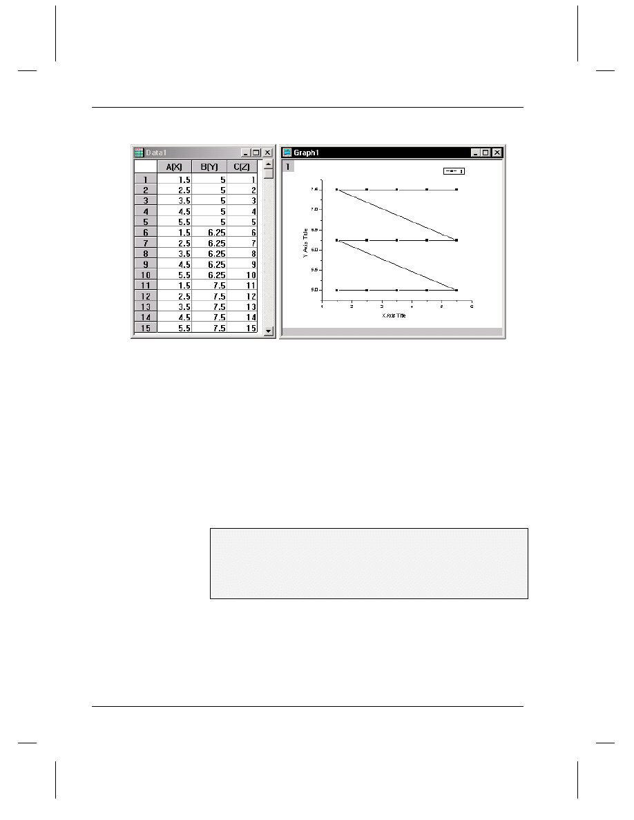
Tutorial 5, Creating 3D Surface Graphs

164

•

Converting a Worksheet to a Matrix

Figure 6: Plotting Worksheet Data to Check Regularity

=> Sparse XYZ: This method converts “regular” XYZ data to a matrix
by assuming missing values for missing X,Y data pairs.
=> Random XYZ: If your worksheet data does not fall into any of the
previously mentioned types, then it can be classified as random data.
The procedure for converting random XYZ data to a matrix is called
gridding. Origin offers a number of gridding methods, including the
method of Renka and Cline and a modification of Shepard's method.
Both these methods are provided by the NAG® C Library eo1
Interpolation.

The data in this lesson is an XYZ worksheet with un-ordered XY data.
Thus, random gridding will be used to convert the data to a matrix.

To Convert the Worksheet to a Matrix:
1) If it is not still selected, click on the C(Z) column heading to select
the column.
2) Select Edit:Convert to Matrix:Random XYZ. This opens the
Random XYZ Gridding dialog box.

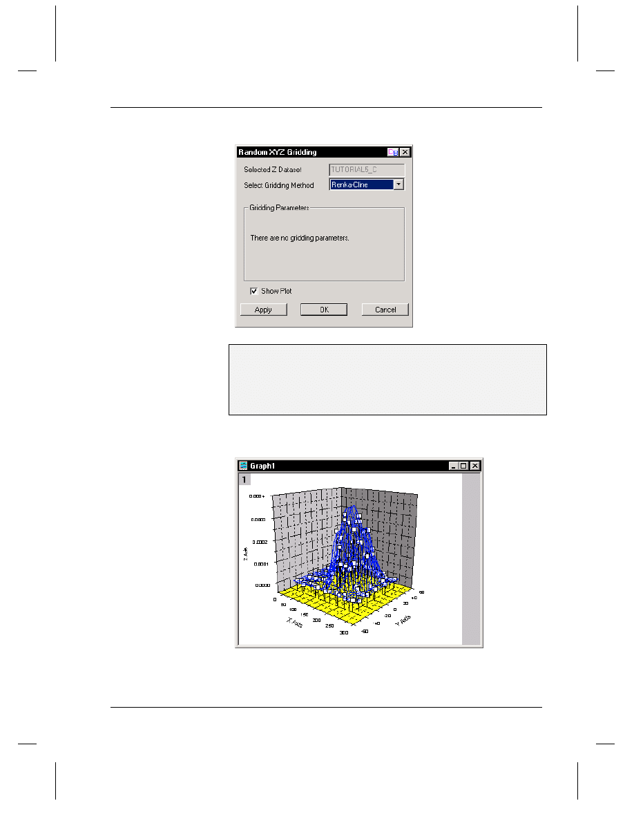
Tutorial 5, Creating 3D Surface Graphs

Converting a Worksheet to a Matrix

•

165

Figure 7: The Random XYZ Gridding Dialog Box

3) Select Renka-Cline from the Select Gridding Method drop-down list
if it is not already selected.
4) Select the Show Plot button if it is not already selected.
5) Click Apply. A graph is created that shows the raw data as an XYZ
scatter plot and the grid as a mesh plot.

Figure 8: Gridding Using the Renka-Cline Method

By changing the gridding method and re-clicking Apply, you can
compare the graph output for the various methods and then choose the

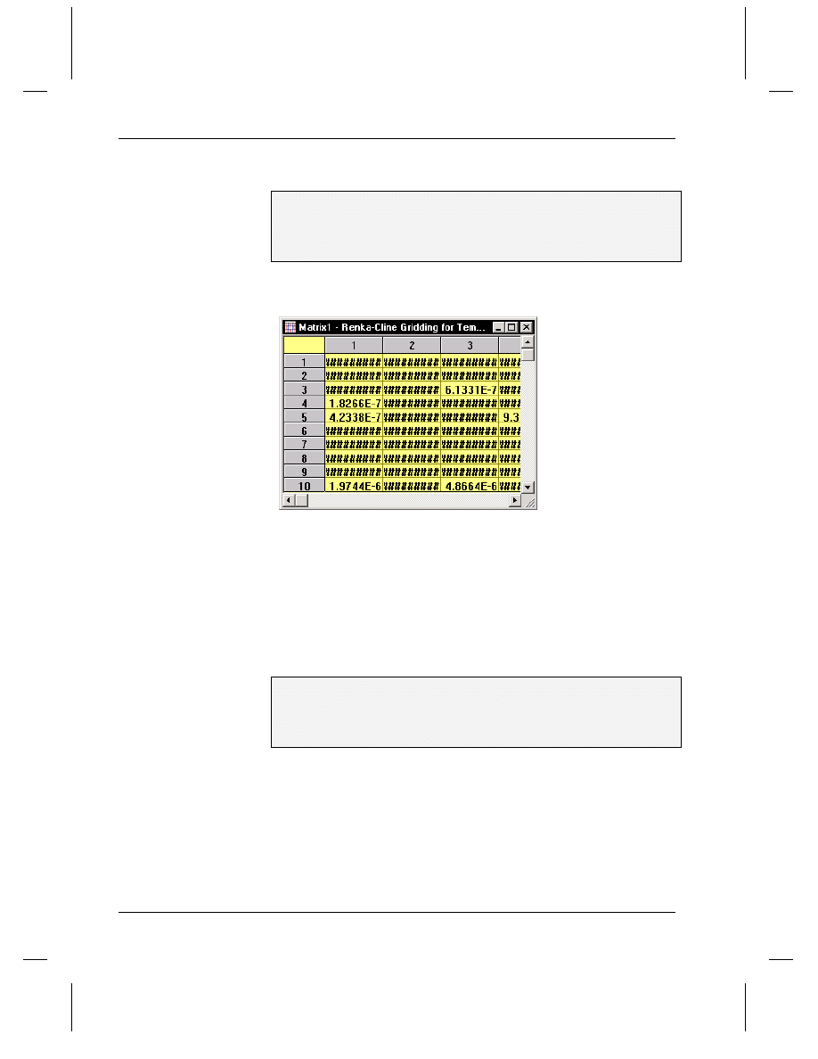
Tutorial 5, Creating 3D Surface Graphs

166

•

Creating a 3D Surface Graph

method which produces a surface that best includes the points. For this
data, the Renka-Cline method is the best choice.

6) Click OK to close the dialog box.
7) Activate the matrix window for the Renka-Cline gridding. (Note that
if Origin cannot display an entire cell value, it displays # characters in the
cell.)

Figure 9: The Matrix Containing the Gridding Results

Creating a 3D Surface Graph

Now that you have your data in a matrix you can create any type of
contour or 3D surface graph. For this tutorial you will create a 3D color
mapped surface graph.

To Create a 3D Color Mapped Surface Graph:
1) With the matrix active, select Plot:3D Color Map Surface. A
Reminder Message opens informing you that the graph will be displayed
using Speed Mode.

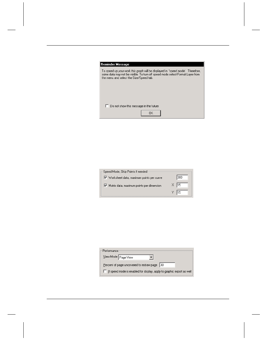
Tutorial 5, Creating 3D Surface Graphs

Creating a 3D Surface Graph

•

167

Figure 10: A Reminder Message about Speed Mode

Speed Mode increases the redraw speed of your graph by displaying a
reduced number of data points. You can control the Speed Mode setting
by selecting Format:Layer to open the layer's Plot Details dialog box.
Then select the Size Speed tab and edit the Speed Mode, Skip Points if
Needed group.

Figure 11: Setting Speed Mode to Increase the Graph Redraw Speed

This Speed Mode setting only effects the view of the graph in Origin.
When you copy, export, or print your graph, all the data points will be
included. To use Speed Mode when you export or copy your graph,
select Format:Page to open the page's Plot Details dialog box. Then
select the Miscellaneous tab and edit the Performance group.

Figure 12: Setting Speed Mode for Exporting or Copying a Graph

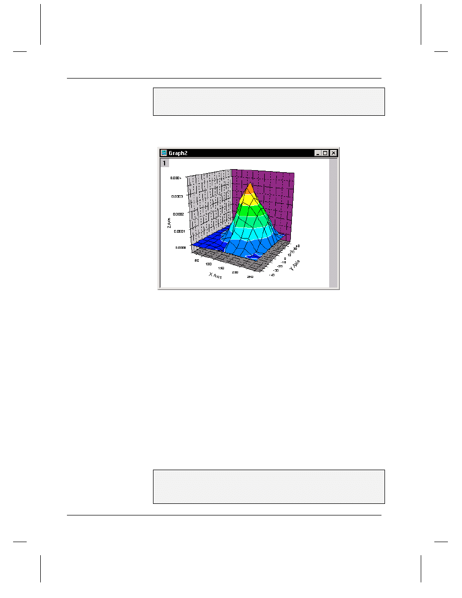
Tutorial 5, Creating 3D Surface Graphs

168

•

Customizing the Graph

2) Click OK to close the Reminder Message. The matrix data is plotted
as a color map surface graph. The different colors represent different Z-
value ranges.

Figure 13: Color Map Surface Graph

Customizing the Graph

Origin gives you full control over the color mapping applied to the
surface data plot. All the options for customizing the color map are
located on the Color Map tab of the Plot Details dialog box.

Changing the Color Map Values

The Color Map tab on the Plot Details dialog box displays the current
color map associated with levels of Z values. To edit an individual level
or color, click on the value or color in the Level or Fill column. To edit
the entire range of levels or colors, click on the Level or Fill column
heading. To edit a range of levels, SHIFT + click on the desired values
to select a range, then click on the Level or Fill column heading.

To Change the Number of Levels in the Color Map:
1) Right-click on the surface plot.
2) Select Plot Details from the shortcut menu.

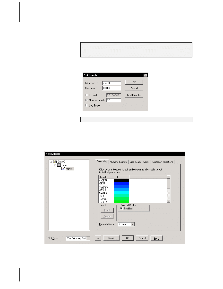
Tutorial 5, Creating 3D Surface Graphs

Customizing the Graph

•

169

3) Click on the Level column heading to open the Set Levels dialog box.
4) Select the Num. of Levels radio button, then type 12 in the associated
text box.

Figure 14: The Set Levels Dialog Box

5) Click OK.

The Color Map tab updates to show twelve levels (plus levels for values
above and below the maximum and minimum levels) and associated
colors in the list box.

Figure 15: Updated Color Map Tab

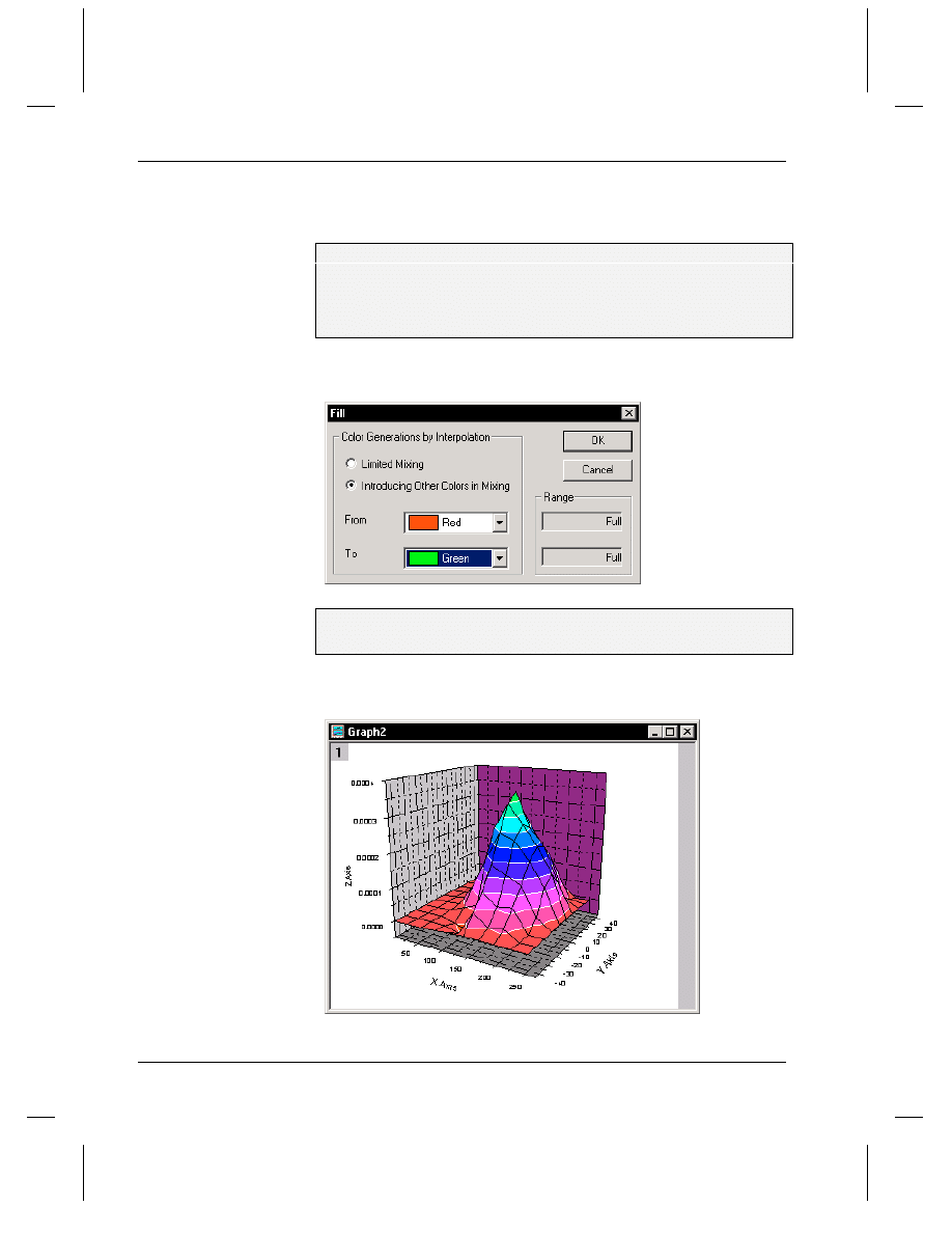
Tutorial 5, Creating 3D Surface Graphs

170

•

Customizing the Graph

Changing the Color Map Colors

Customizing the Fill Color Range:
1) Click on the Fill column heading to open the Fill dialog box.
2) Select Red from the From drop-down list.
3) Select Green from the To drop-down list.

Figure 16: Editing the Fill Dialog Box

4) Click OK.
5) Click OK in the Plot Details dialog box.

Figure 17: The Customized Surface Graph

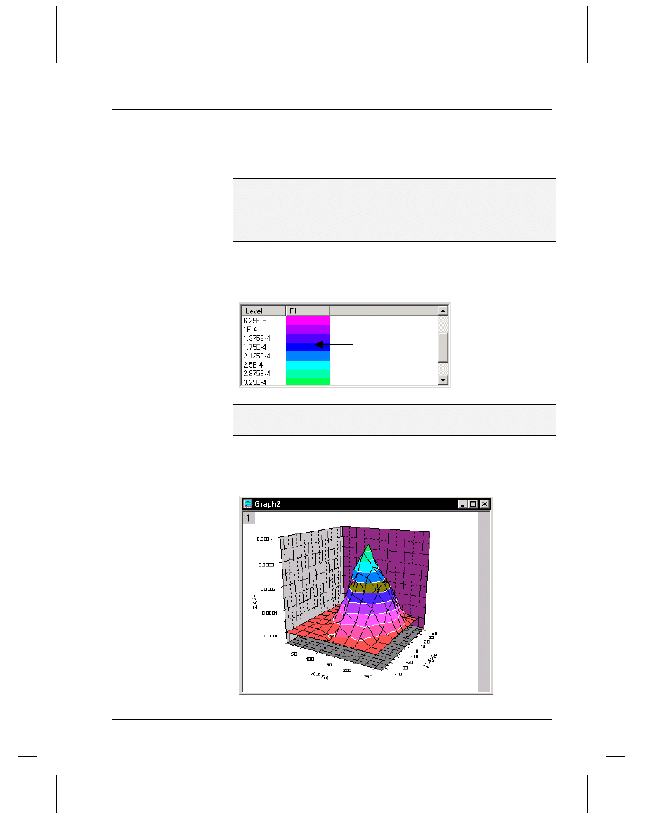
Tutorial 5, Creating 3D Surface Graphs

Customizing the Graph

•

171

In addition to editing color ranges, you can edit individual colors. This is
especially useful if you have an important section of your data that you
want to highlight or make transparent.

To Edit an Individual Color:
1) Right-click on the surface plot.
2) Select Plot Details from the shortcut menu.
3) On the Color Map tab, click on the color associated with 1.75E -4.

The Fill dialog box opens.

Figure 18: Selecting an Individual Color to Edit

Click here.

4) Select None from the Fill Color drop-down list, then click OK.
5) Click OK in the Plot Details dialog box.

The data plot redraws showing the transparent level.

Figure 19: Editing an Individual Color

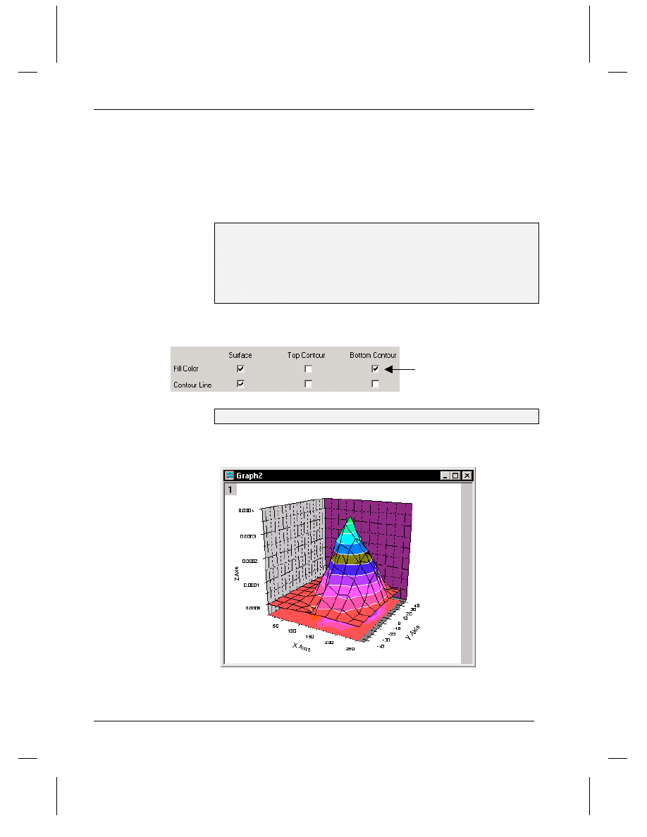
Tutorial 5, Creating 3D Surface Graphs

172

•

Customizing the Graph

Adding Contours to the Color Map Surface
Graph

To further enhance your graph, you can display contour lines and colors
on the top or bottom plane of your surface graph. This is done on the
Surface / Projections tab of the Plot Details dialog box.

To Add Contour Colors to the Bottom Plane of the Surface Graph:
1) Right-click on the surface graph.
2) Select Plot Details from the shortcut menu.
3) Select the Surface / Projections tab.
4) Select the Fill Color check box under the Bottom Contour text.

Figure 20: The Surface / Projections Tab

Select this check box.

5) Click OK.

Figure 21: Displaying Bottom Contour Colors

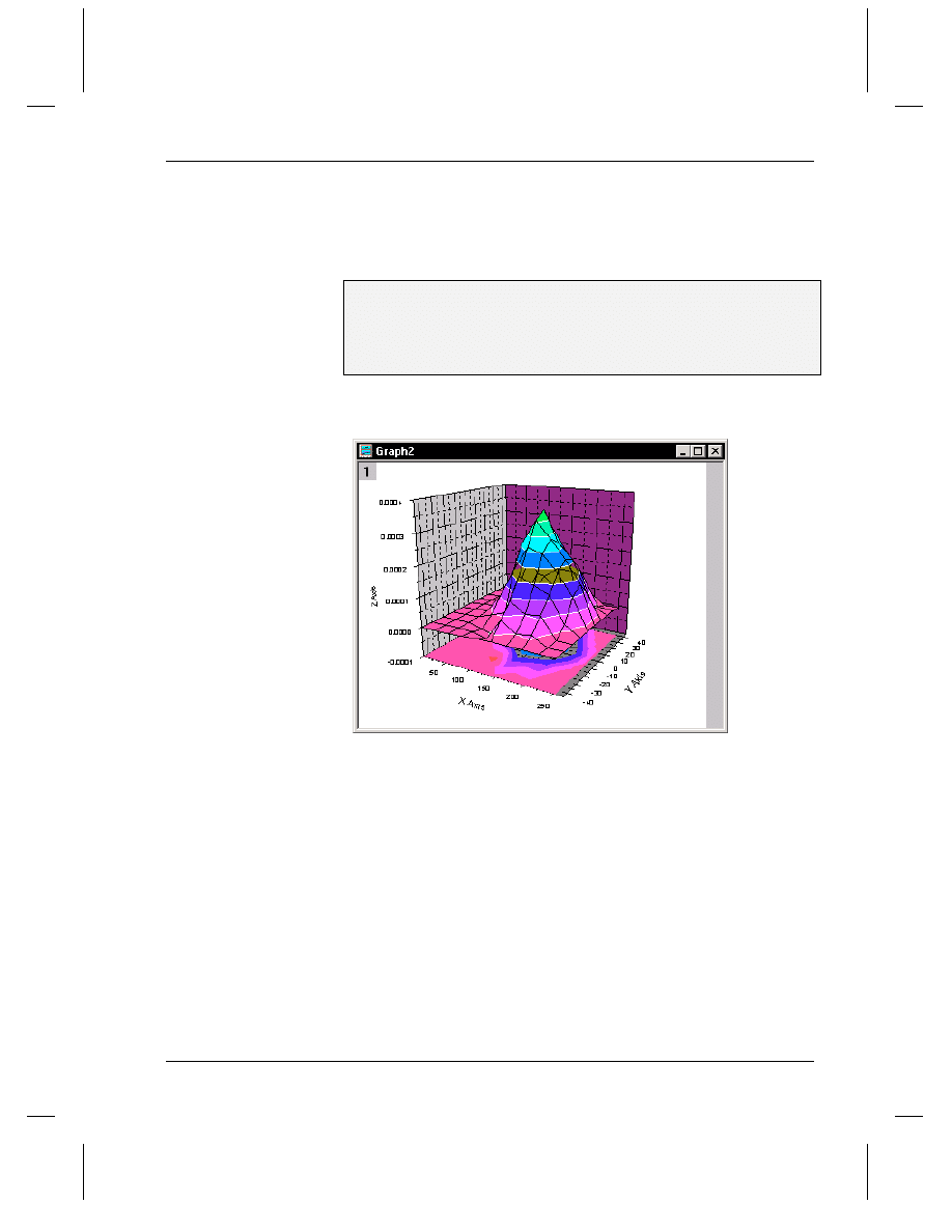
Tutorial 5, Creating 3D Surface Graphs

Customizing the Graph

•

173

With the current Z axis scale range and the current view angle, the
surface plot substantially overlaps the bottom contour, blocking it from
view. To make more of the contour visible, you can change the Z axis
scale to begin from a lower value.

To Change the Z Axis Scale:
1) Select Format:Axes:Z Axis to open the Z Axis dialog box.
2) In the From text box, type -1E-4.
3) Click OK.

Figure 22: Changing the Z Axis Scale

The Z axis now displays a greater range below the surface graph. This
decreases the amount of overlap of the surface plot and the contour,
providing for a better visual presentation.

Changing the Perspective of the Graph

When you create a 3D graph, the 3D Rotation toolbar automatically
opens. This toolbar contains buttons for controlling the perspective of
the 3D graph. By rotating the graph you can further reduce the overlap
of the surface plot with the contour, providing better perspective for
viewing the graph.

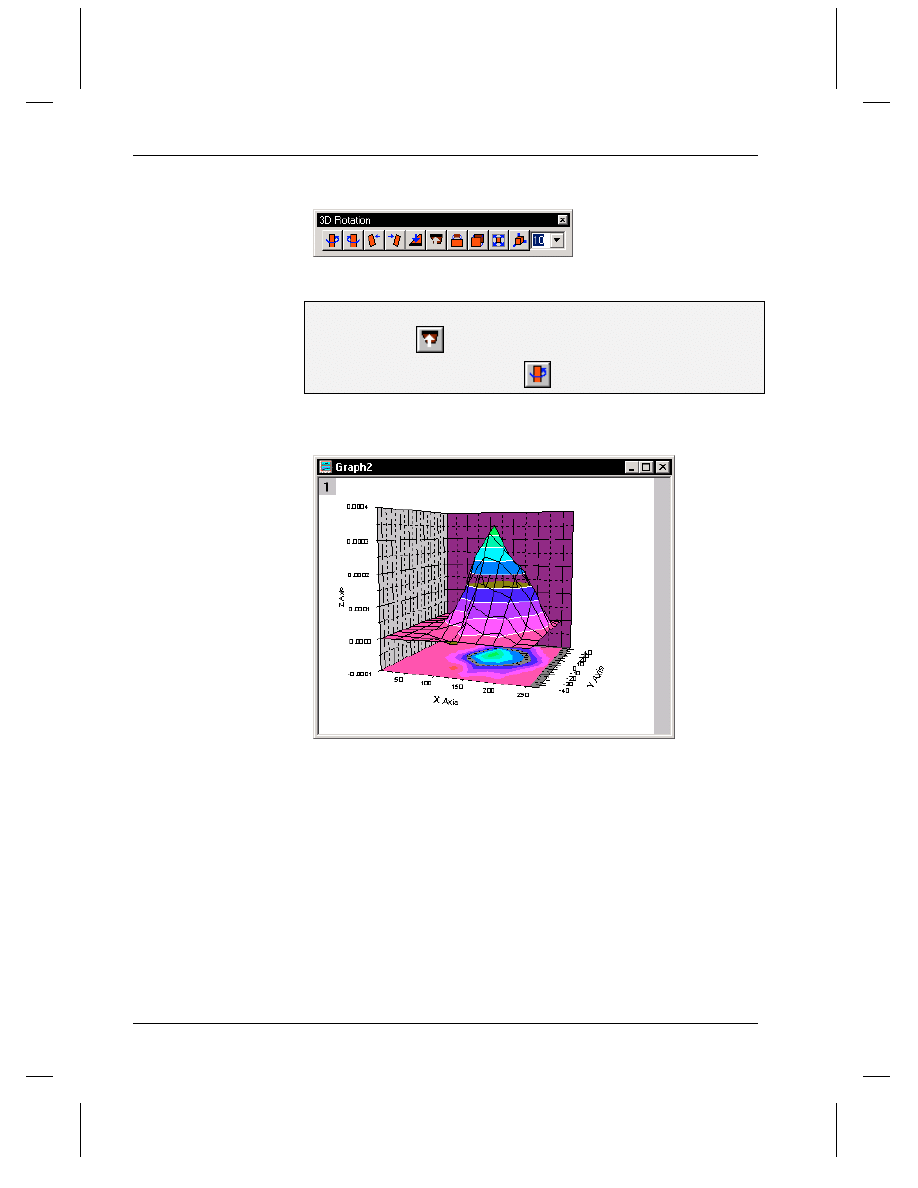
Tutorial 5, Creating 3D Surface Graphs

174

•

Customizing the Graph

Figure 23: The 3D Rotation Toolbar

To Rotate the Graph:

1) Click Tilt Up

on the 3D Rotation toolbar.

2) Click Rotate Counterclockwise

on the 3D Rotation toolbar.

Figure 24: Rotating the Graph

This new perspective eliminates the overlap between the surface plot and
the contour, and provides better visibility of the transparent section of the
surface plot.

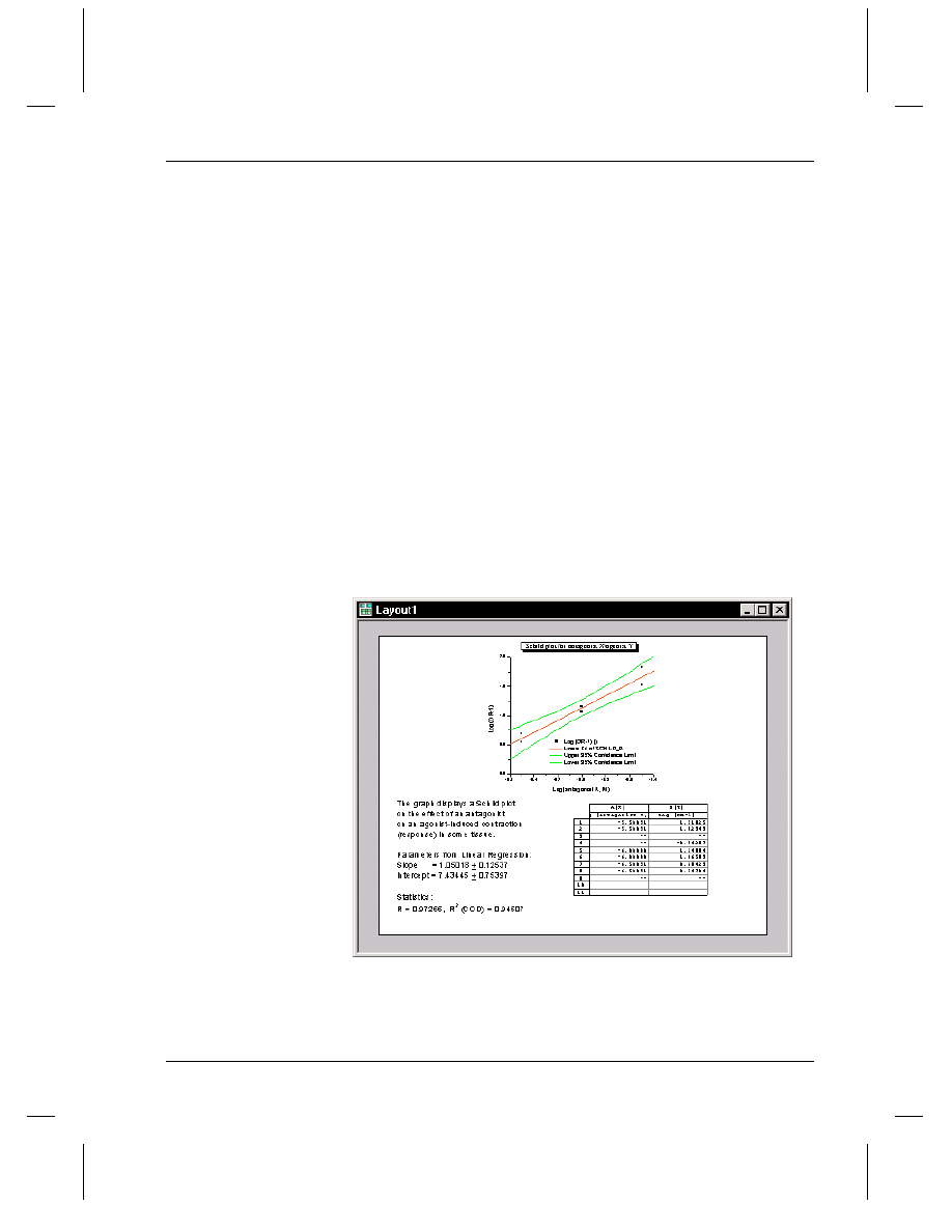
Tutorial 6, Creating Presentations with the Layout Page

Introduction

•

175

Tutorial 6, Creating

Presentations with the Layout
Page

Introduction

Origin provides a layout page for displaying and arranging pictures of
worksheets and graphs from other windows in your project, as well as
text and other annotations.

Figure 1: Example Layout Page with Added Pictures and Text

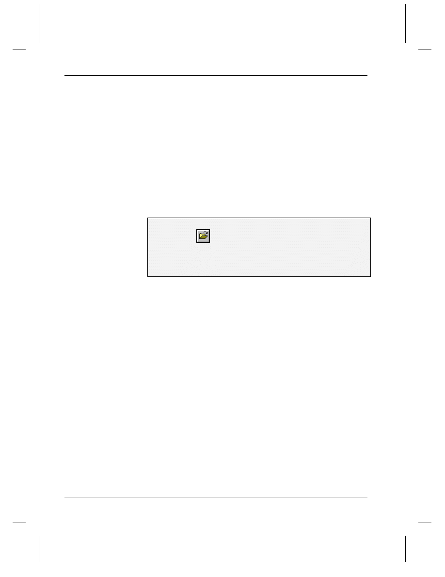
Tutorial 6, Creating Presentations with the Layout Page

176

•

Adding Graphs, Worksheets and Text to the Layout Page

Adding Graphs, Worksheets and Text to the
Layout Page

Pictures of graphs and worksheets are added to the layout page by
clicking the buttons on the Layout toolbar, or by selecting associated
menu commands. Text can be added with the Text tool, or by pasting
from the Clipboard. Shapes, lines, and arrows can be added using the
drawing tools from the Tools toolbar.

Opening the Project File

The data for this tutorial lesson is provided in an Origin project file.

To Open the Project File:

1) Click Open

on the Standard toolbar.

2) In the Origin \SAMPLES\GRAPHING\STATISTICAL GRAPHS
folder, select HISTOGRAM.OPJ from the list of files.
3) Click Open.

A project opens displaying a notes window and a histogram in a graph
window. Other windows are available in the current Project Explorer
folder and in other folders.

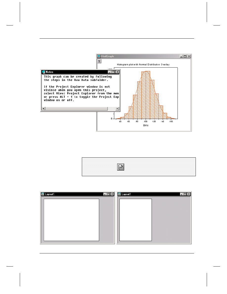
Tutorial 6, Creating Presentations with the Layout Page

Adding Graphs, Worksheets and Text to the Layout Page

•

177

Figure 2: The Histogram Project File

Creating a New Layout Page

To Create a New Layout Page:

1) Click New Layout

on the Standard toolbar. A blank layout page

opens.

Figure 3: New Layout Page in Landscape vs. Portrait Orientation

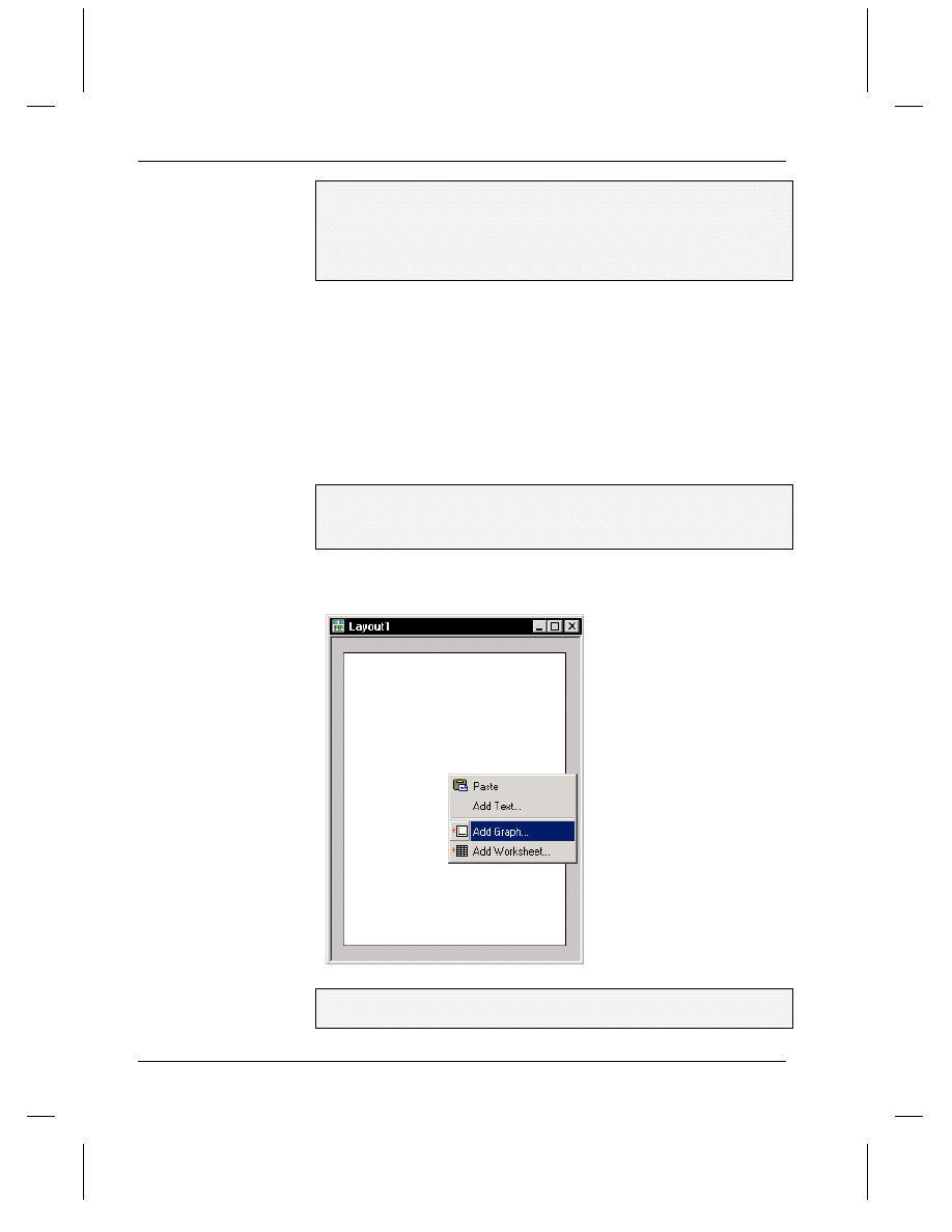
Tutorial 6, Creating Presentations with the Layout Page

178

•

Adding Graphs, Worksheets and Text to the Layout Page

2) If the layout page is displayed in the landscape orientation, right-click
on the gray area of the layout page, then select Rotate Page from the
shortcut menu that opens. The layout page should now display in portrait
orientation.
3) Resize the layout page window if needed.

Adding Pictures and Text to a Layout Page

You can add pictures of worksheets and graphs that are currently in your
project to a layout page. After you add a picture, if you want to change
the details of the picture (for example, changing a line data plot to a
scatter data plot), you must make the changes in the source window.
After you do this, the picture in the layout page will update to reflect
your changes.

To Add Pictures of Graphs and Worksheets to the Layout Page:
1) Right-click in the layout page and select Add Graph from the
shortcut menu.

Figure 4: Adding a Graph Picture to the Layout Page

2) Select HistGraph from list box in the Select Graph Object dialog box
and click OK.

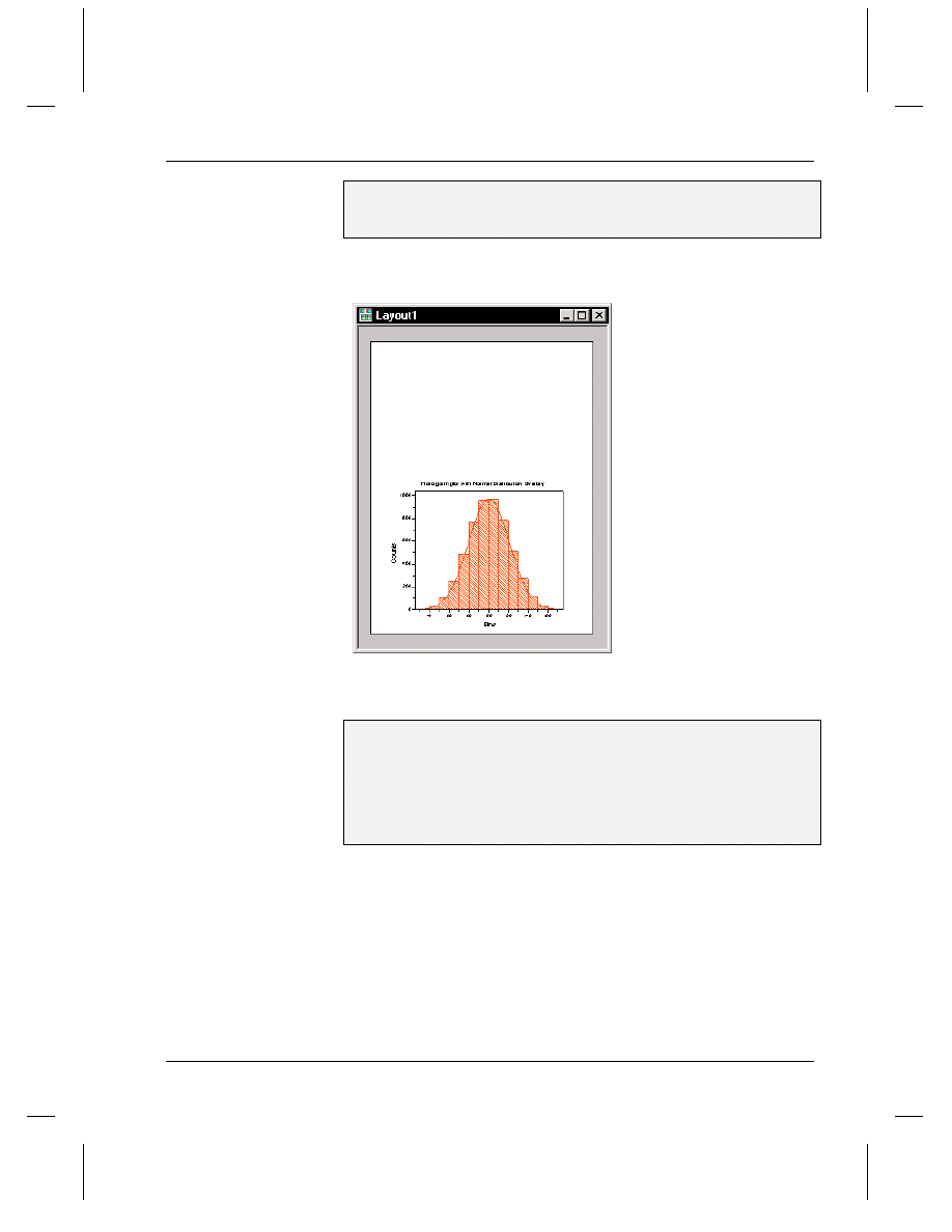
Tutorial 6, Creating Presentations with the Layout Page

Adding Graphs, Worksheets and Text to the Layout Page

•

179

3) Drag out a box on the bottom half of the layout page. After you
release the mouse button, a picture of the HistGraph graph displays in the
layout page.

Figure 5: Adding a Graph Picture to the Layout Page

When the graph picture is selected, you can drag the picture to a new
location or use the sizing handles to resize it.

4) Right-click on a blank section of the layout page and select Add
Worksheet from the shortcut menu.
5) Select Bin1 from the list box in the Select Worksheet Object dialog
box and click OK.
6) Drag out a box in the top half of the layout page, leaving some space
at the top for a title.

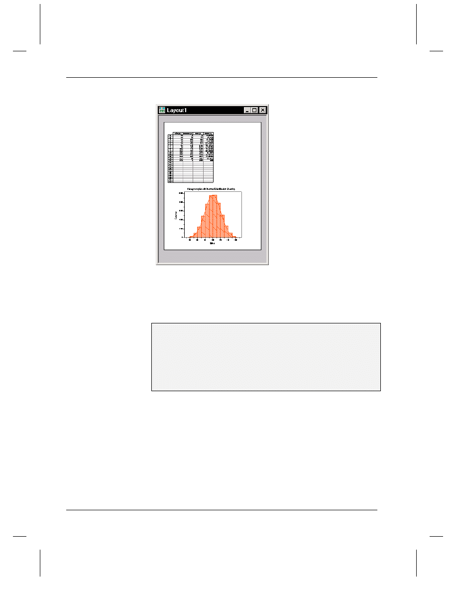
Tutorial 6, Creating Presentations with the Layout Page

180

•

Adding Graphs, Worksheets and Text to the Layout Page

Figure 6: Adding a Worksheet Picture to the Layout Page

After you add the worksheet picture to the layout page, it may display a
blank area to the right of the last worksheet column, and it may include a
number of blank worksheet rows. To remove these blanks areas in the
picture, you can disable the "keep aspect ratio" setting and resize the
picture as desired.

7) Right-click on the worksheet picture in the layout page and select
Keep Aspect Ratio from the shortcut menu. This de-selects the
command.
8) Drag one of the control handles on the right edge of the worksheet
picture so that only the four worksheet columns display.
9) Drag one of the control handles on the bottom edge of the worksheet
picture so that only the worksheet rows with values display.

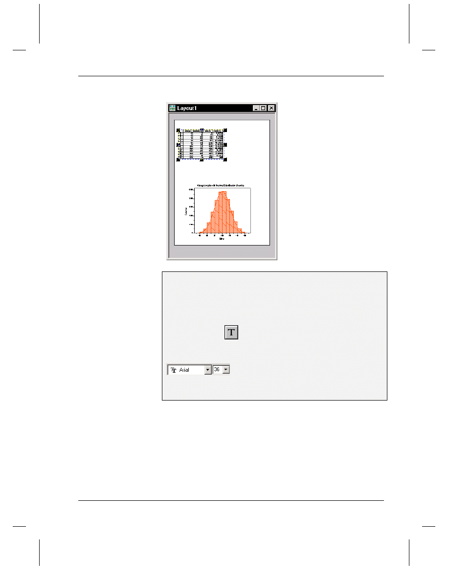
Tutorial 6, Creating Presentations with the Layout Page

Adding Graphs, Worksheets and Text to the Layout Page

•

181

Figure 7: Resizing the Worksheet Picture

10) Re-position the worksheet picture in the layout page.
11) Click off the worksheet picture (but in the layout page) to de-select
the picture.

To Add Text to the Layout Page using the Text Tool:

1) Click Text Tool

on the Tools toolbar.

2) Click above the worksheet picture in the layout page.
3) Before you start typing, select 36 from the Style combo box

4) Then type Histogram Data.
5) Click off the label to exit the editing mode.

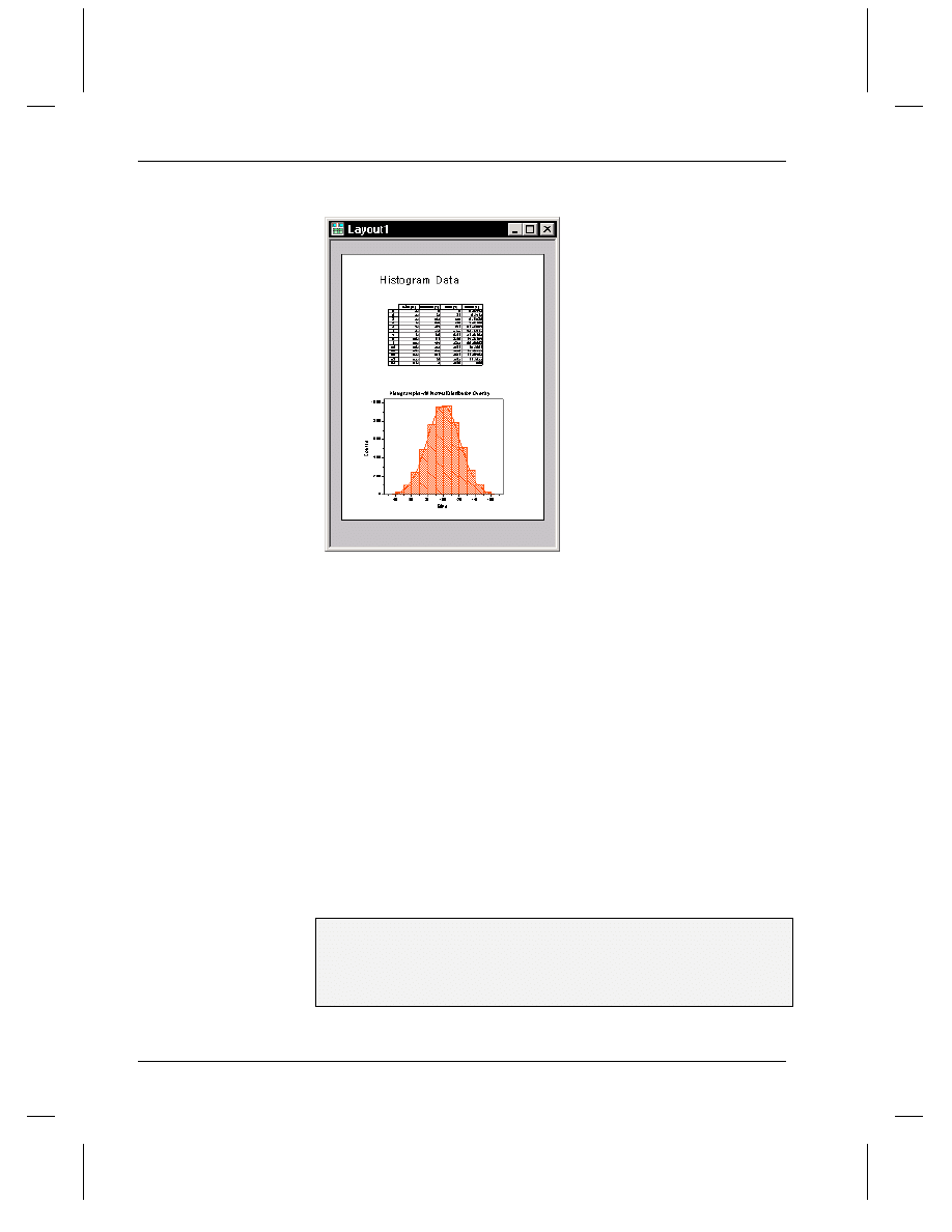
Tutorial 6, Creating Presentations with the Layout Page

182

•

Customizing the Appearance of the Layout Page

Figure 8: Adding Text to the Layout Page

Customizing the Appearance of the Layout
Page

In this section, you will fine tune the position of the pictures displayed in
the layout page. In addition, you will make changes to the source graph
window to change the picture's appearance in the layout page.

Arranging Pictures on the Layout Page

There are several ways to arrange pictures on the layout page. You can
drag the pictures and estimate the position, use the Object Edit toolbar, or
view the grid (View:Show Grid) on the layout page and align the
pictures using the grid lines as a guide.

To Arrange the Pictures on the Layout Page Using the Object Edit Tools:
1) If the Object Edit toolbar is not currently open, select View:Toolbars,
select the Object Edit check box on the Toolbars tab, then click Close.
2) Click on the Histogram Data text label to select it.

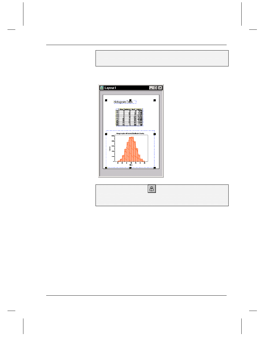
Tutorial 6, Creating Presentations with the Layout Page

Customizing the Appearance of the Layout Page

•

183

3) Press SHIFT and click on the worksheet picture and then on the graph
picture (in that order). All three objects are now selected in the layout
page.

Figure 9: Selecting the Objects in the Layout Page

4) Click the Vertical button

on the Object Edit Toolbar. The

pictures align vertically using the last selected picture (the graph).
5) Click in the layout page but off the pictures to de-select them.

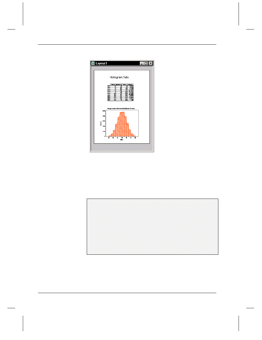
Tutorial 6, Creating Presentations with the Layout Page

184

•

Customizing the Appearance of the Layout Page

Figure 10: Arranging the Objects on the Layout Page

Editing the Pictures in the Layout Page

Although you cannot edit the worksheets and graphs in the layout page
directly, Origin provides a shortcut menu command to go to the source
window.

To Edit a Source Window from the Layout Page:
1) Right-click on the graph picture in the layout page.
2) Select Go To Window from the shortcut menu. Origin makes the
HistGraph window active.
3) Right-click on the histogram and select Plot Details from the shortcut
menu.
4) Select the Data tab.
5) Clear the Automatic Binning check box.
6) Type 5 in the Bin Size combo box.

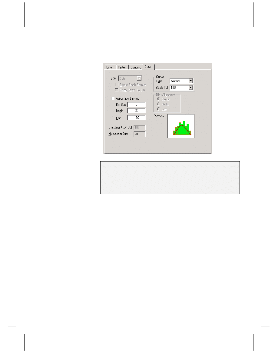
Tutorial 6, Creating Presentations with the Layout Page

Customizing the Appearance of the Layout Page

•

185

Figure 11: Modifying the Number of Bins

7) Click OK.
8) Double-click on the Y axis in the HistGraph window. This opens the
Y Axis dialog box.
9) Select the Scale tab if it is not currently selected.
10) Type 600 in the To text box and 100 in the Increment text box.

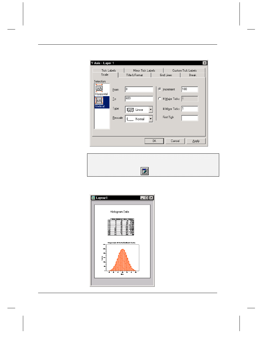
Tutorial 6, Creating Presentations with the Layout Page

186

•

Customizing the Appearance of the Layout Page

Figure 12: Modifying the Axis Scale

11) Click OK.
12) Activate the layout page window.

13) Click the Refresh button

on the Standard toolbar.

Figure 13: Updating the Layout Page

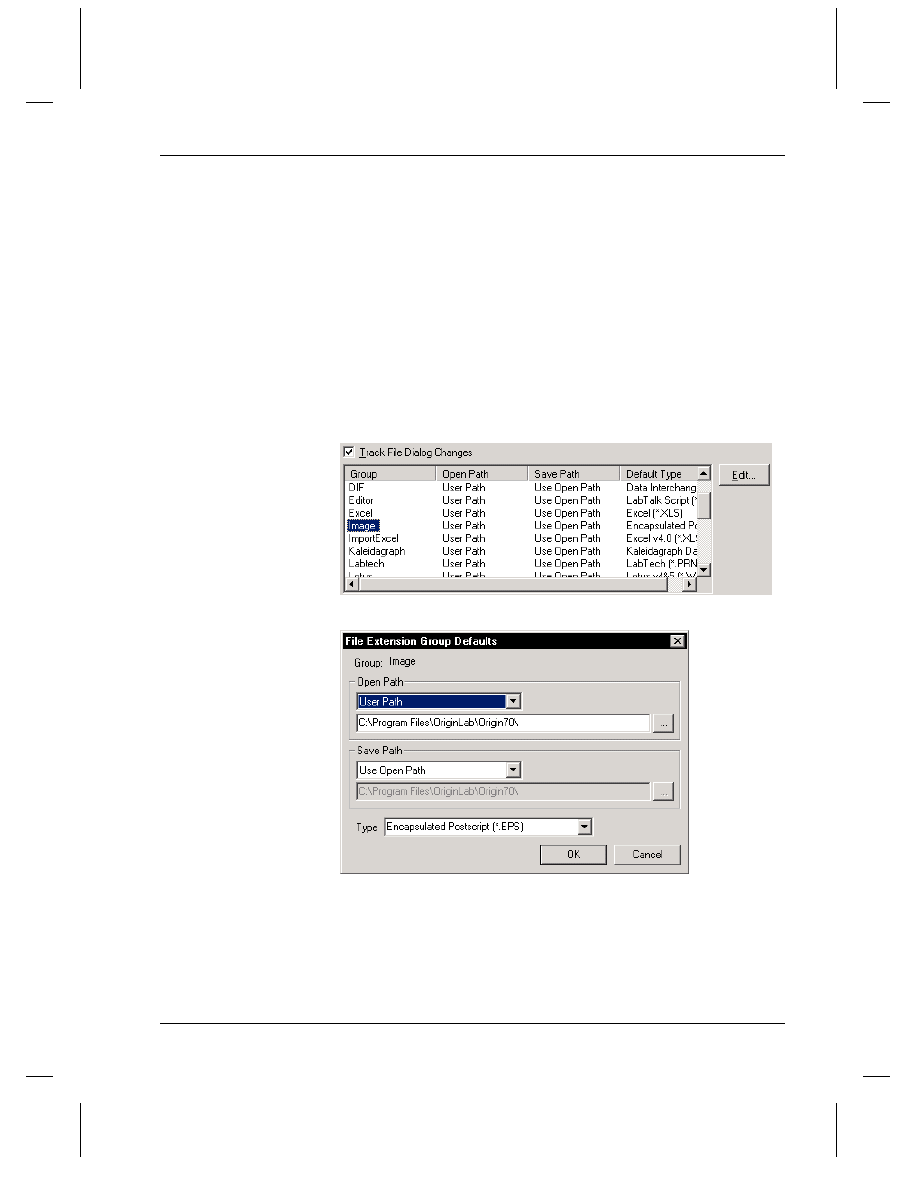
Tutorial 6, Creating Presentations with the Layout Page

Exporting the Layout Page

•

187

Exporting the Layout Page

In addition to customizing your layout page presentation in Origin, you
can export the layout page into other applications. Origin provides a
number of raster and vector graphic export filters. In addition, you can
copy the layout page to the Clipboard and paste it into other applications.
When exporting a layout page or graph to a file, Origin tracks the
previous save location and displays that folder by default in the Save As
dialog box. To modify this behavior, select Tools:Options to open the
Options dialog box. Then select the File Locations tab. Select Image
from the top list box and then click the Edit button.

Figure 14: Customizing the Default File Save Folder

To store your image file in the same location as the open Origin project
file, select Project Path from the Save Path drop-down list. (Note that
you can also select the default image type that will display in the Save As
dialog box.) Click OK in this dialog box and in the Options dialog box.
To save the settings for the next Origin session, click Yes at the Attention
prompt.

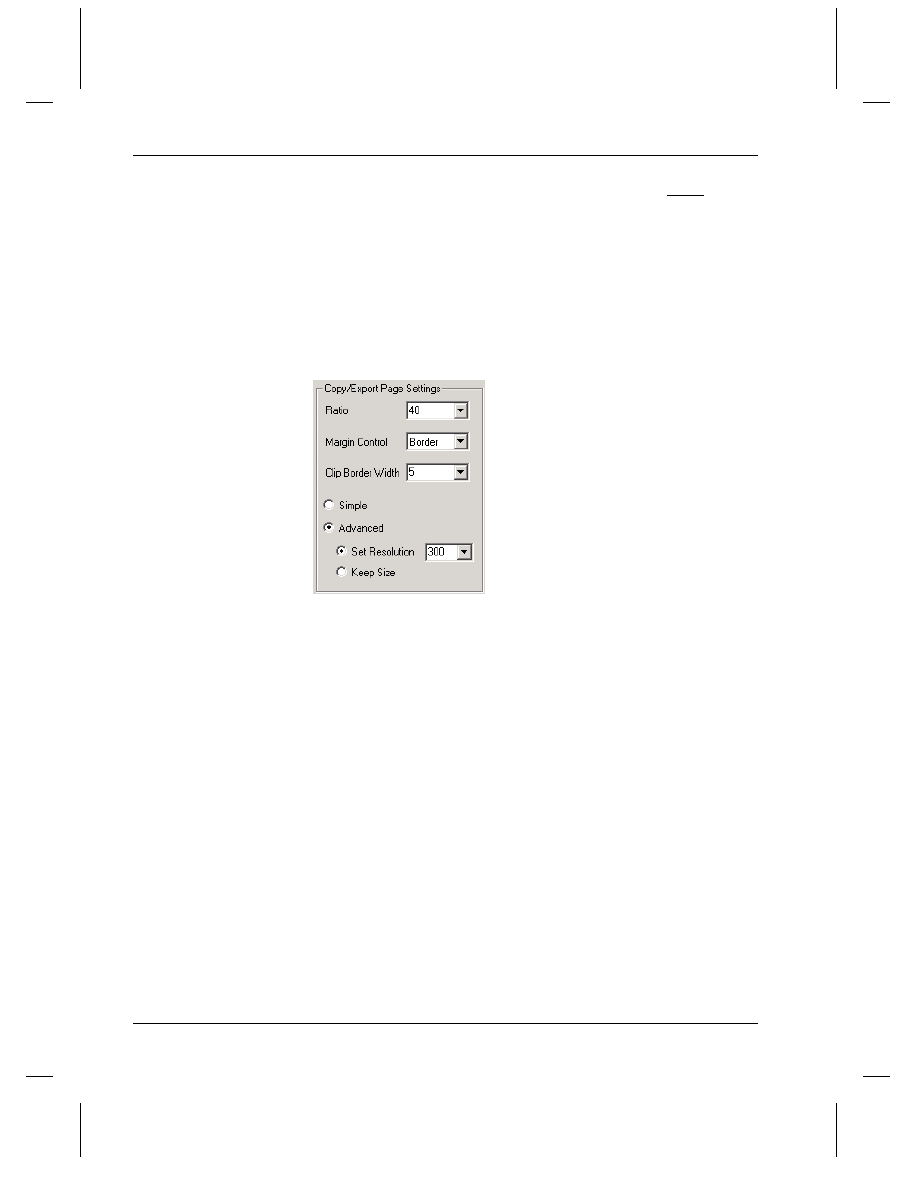
Tutorial 6, Creating Presentations with the Layout Page

188

•

Exporting the Layout Page

This discussion also
applies to graph
windows.

When you copy to the Clipboard and when you export to a vector image
format (Adobe Illustrator (AI), Computer Graphics Metafile (CGM),
AutoCAD Drawing Interchange (DXF), Encapsulated PostScript (EPS),
Enhanced Metafile (EMF), Macintosh PICT (PCT), Portable Document
Format (PDF), and Windows Metafile (WMF)), Origin uses settings in
the Options dialog box (Tools:Options) to determine the size of the
picture when pasted or inserted into another application. These settings
are located on the Page tab.

Figure 15: Default Copy Page and Export Settings

The Ratio combo box controls the size of the picture when pasted or
inserted into another application. The units are as a percentage of the
page size in Origin. Thus, if you want the inserted picture to be 25% of
the page size in Origin, set this combo box to 25. (To set the layout page
size in Origin, select Format:Layout Page to open the Plot Details
dialog box. Then edit the Print Dimensions tab.)
The Margin Control drop-down list controls the amount of the page that
is copied or exported. The options are Border, Tight, and Page. The
Border and Tight options use a bounding box to control the amount of
page that is included. The bounding box is determined by the smallest
rectangular box required to completely encompass all objects on the
page.
=> Select Border to copy or export the page within the bounding box
plus add the border that is specified in the Clip Border Width combo box.
The Clip Border Width value is a percentage of the width of the
bounding box.
=> Select Tight to copy or export the page within the bounding box.
=> Select Page to copy or export the entire page.

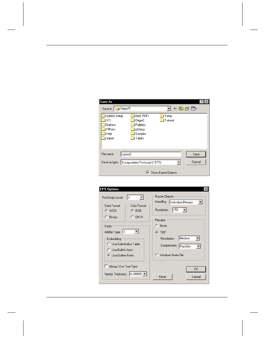
Tutorial 6, Creating Presentations with the Layout Page

Exporting the Layout Page

•

189

The Options dialog box picture size settings are global preferences. Your
custom settings will be used for the current Origin session and for future
sessions (if you "Save as Origin's Startup Options"). In addition, both the
vector and raster export image formats provide format-specific export
options. These options are accessible by selecting the Show Export
Options check box in the Save As dialog box (File:Export Page).

Figure 16: Accessing the Export Options

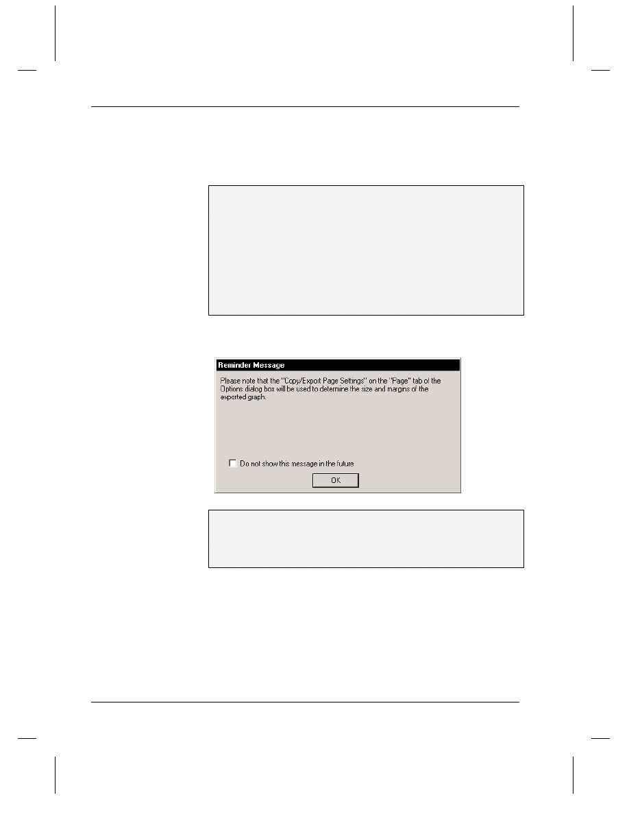
Tutorial 6, Creating Presentations with the Layout Page

190

•

Exporting the Layout Page

If you change these image export settings, Origin will remember and use
the settings the next time you export using the same format. Thus, you
can clear the Show Export Options check box once you have established
settings appropriate to your needs.

To Export the Layout Page as an Encapsulated PostScript File:
1) Select File:Export Page.
2) Type Presentation1 in the File Name text box.
3) Select Encapsulated PostScript (*.EPS) from the Save As Type drop-
down list.
4) Select the Show Export Options check box.
5) Click Save. A Reminder Message informs you that the settings from
the Options dialog box (Tools:Options) will be used to determine the
picture size.

Figure 17: Reminder Message when Exporting a Vector Format

6) Click OK. The EPS Options dialog box opens.
7) In the Preview group, select the TIFF radio button if it is not currently
selected. (See Figure 16.)
8) Click OK.

The layout page is exported as an EPS file and can be inserted into any
application that recognizes this file type.

Tutorial 7, Working with Excel in Origin

Introduction

•

191

Tutorial 7, Working with Excel in

Origin

Introduction

You can open Excel workbooks directly in Origin, provided you have
Excel 7 or later installed on your computer. This allows you to combine
Excel’s spreadsheet tools with Origin’s powerful graphing and analysis
tools. This tutorial will show you how to open Excel workbooks in
Origin, plot using Origin graph templates, and then save workbooks from
within Origin.

Opening an Excel Workbook in Origin

Note: To perform this tutorial, you must have Excel version 7 or later
installed on your computer either as a local or network copy.

To Open an Existing Excel Workbook:

1) Click New Project

on the Standard toolbar.

2) Click Open Excel

on the Standard toolbar.

3) In the Origin \TUTORIAL folder, select TUTORIAL_7.XLS from the
list of files.
4) Click Open.

The Open Excel dialog box opens. This dialog box allows you to open
your Excel workbook as a workbook in Origin, or as an Origin
worksheet. To use Excel's spreadsheet tools in Origin, you must open as
a workbook.

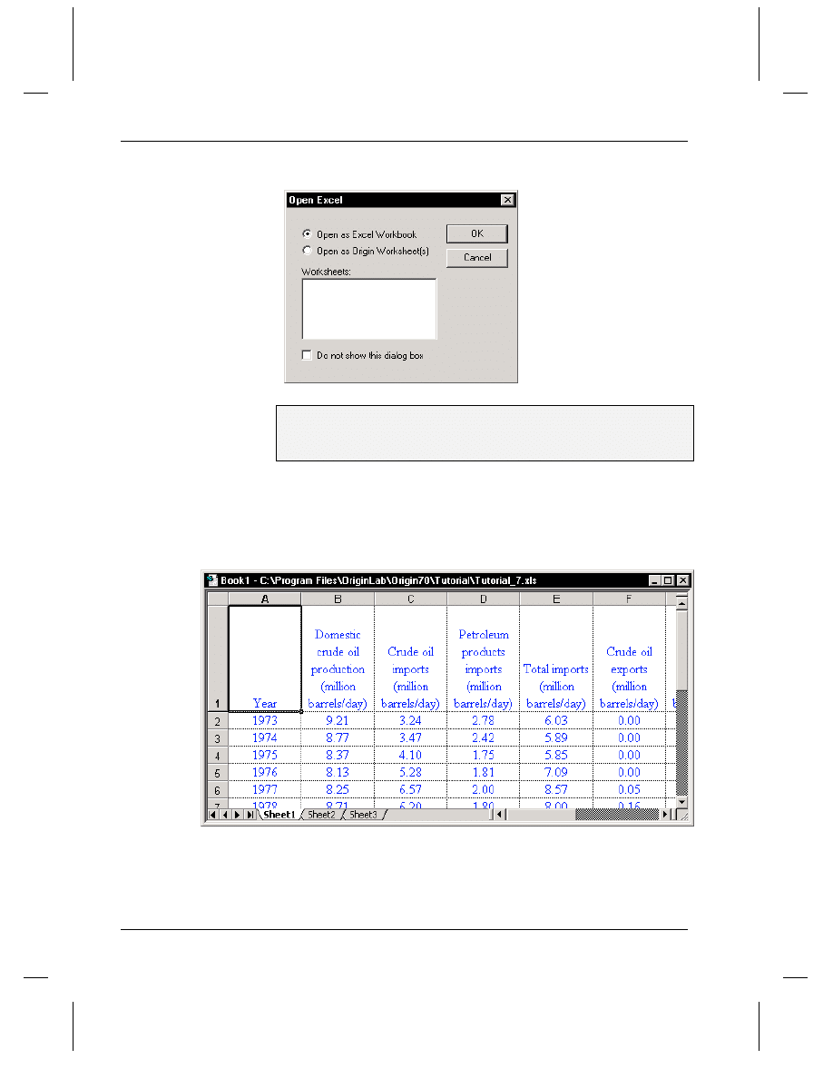
Tutorial 7, Working with Excel in Origin

192

•

Opening an Excel Workbook in Origin

Figure 1: The Open Excel Dialog Box

5) If it is not already selected, select the Open As Excel Workbook radio
button.
6) Click OK.

The workbook opens in the Origin workspace. In addition, a
combination of Origin and Excel menus and toolbars are now displayed
in the workspace.

Figure 2: Opening an Excel Workbook in Origin

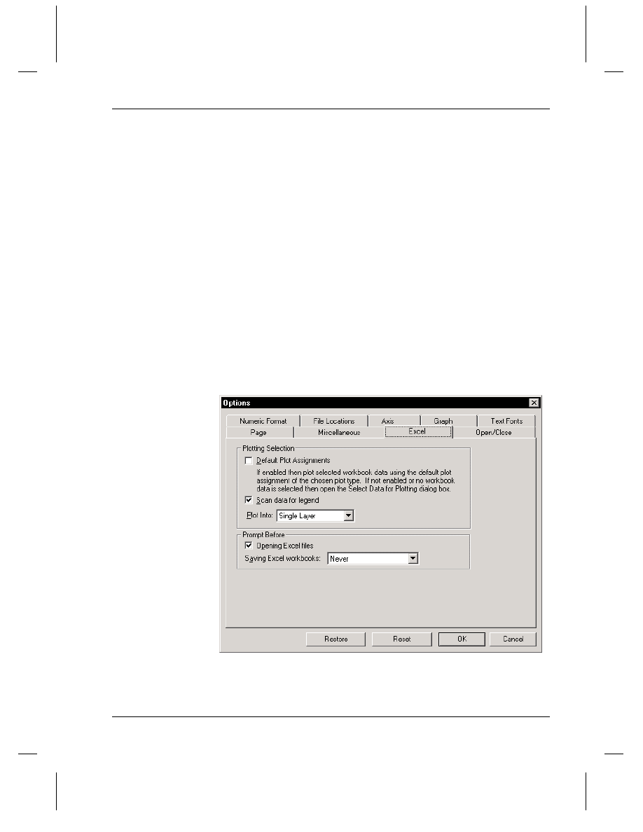
Tutorial 7, Working with Excel in Origin

Plotting an Excel Workbook in Origin

•

193

Plotting an Excel Workbook in Origin

Plotting Excel workbook data in Origin is very similar to plotting Origin
worksheet data. If a graph window is already open, you can drag data
from a workbook into the graph window. You can also create a new
graph from your workbook data by activating your workbook and
clicking a button on one of the plotting toolbars or by selecting a graph
type from the Plot menu. An intermediary Select Data for Plotting
dialog box will open for you to assign data sets. After you get familiar
with Origin's graph templates, you can disable this dialog box and make
your data set selections directly in the workbook.
By default, the Select Data for Plotting dialog box will always open
when an Excel workbook is active and you then click a plotting button or
select a plotting menu command. This dialog box opening behavior is
controlled from the Options dialog box. To open the Options dialog box
when a workbook is active, select Window:Origin Options. When any
other window type is active, select Tools:Options. Then select the Excel
tab.

Figure 3: The Excel Tab of the Options Dialog Box

The Default Plot Assignments check box determines whether or not the
Select Data for Plotting dialog box will open.

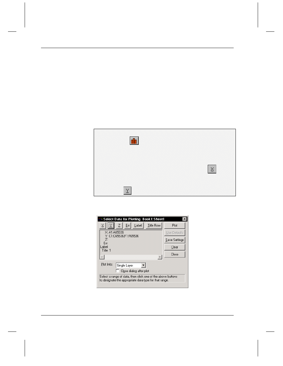
Tutorial 7, Working with Excel in Origin

194

•

Plotting an Excel Workbook in Origin

=> When this check box is cleared (default), the Select Data for Plotting
dialog box will always open for selecting data sets.
=> When this check box is selected, the Select Data for Plotting dialog
box will only open if you did not select any workbook data. Otherwise,
Origin will plot your selected data into a new graph window.

Creating a Graph Using the Select Data for
Plotting Dialog Box

The Select Data for Plotting dialog box lets you select data and then
assign plotting designations.

To Create a Graph Using the Select Data for Plotting Dialog Box:

1) Click Column

on the 2D Graphs toolbar. This opens the Select

Data for Plotting dialog box.
2) Reposition the dialog box so that you can see the column headings in
the Excel workbook.

3) Click the column A heading in the workbook, then click

in the

Select Data for Plotting dialog box.
4) Click the column C heading, then CTRL+click the column F heading

and then click

in the Select Data for Plotting dialog box.

Figure 4: The Select Data for Plotting Dialog Box

The box below the buttons shows the data ranges representing the data
types. X:A1:A65536 means that the X data is being represented by

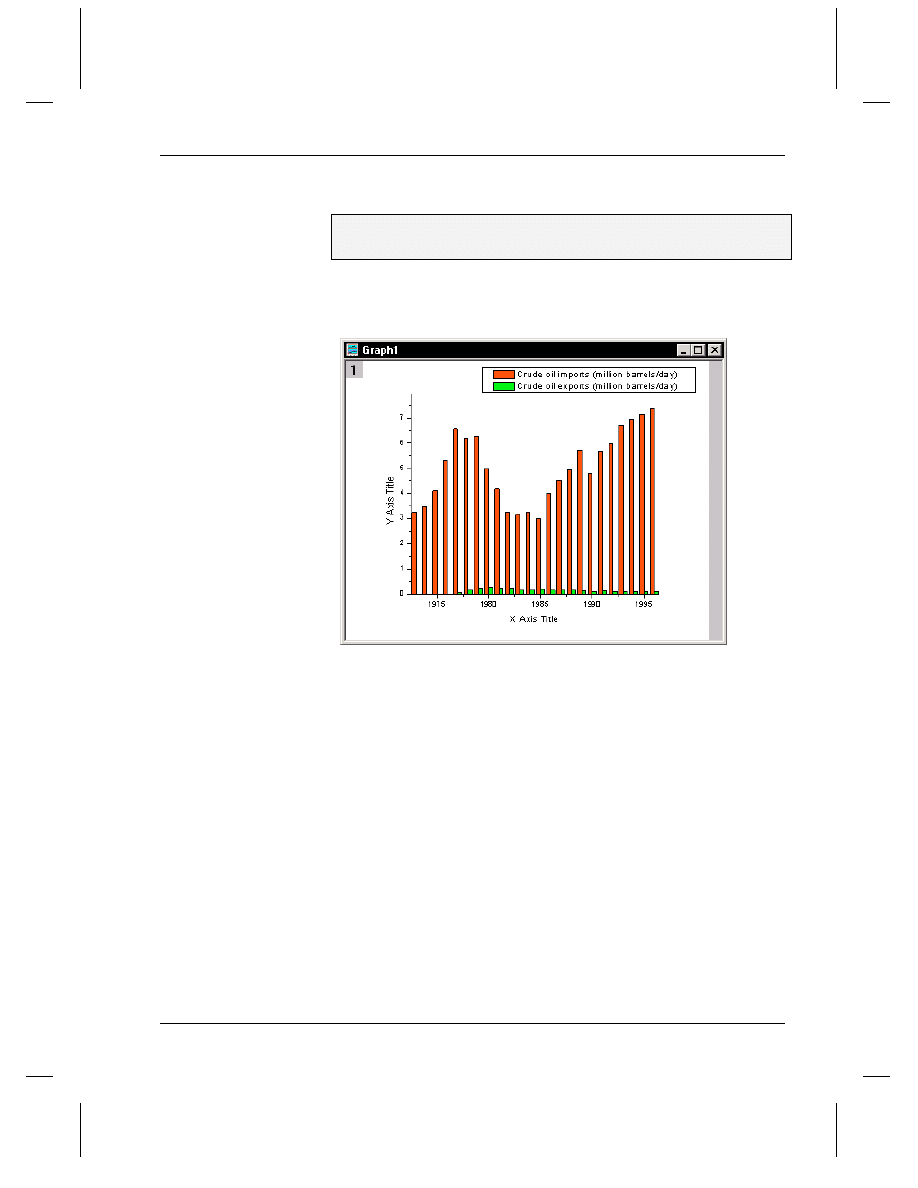
Tutorial 7, Working with Excel in Origin

Plotting an Excel Workbook in Origin

•

195

column A rows 1 to 65536. The last row number of the column is shown
because you selected the whole column.

5) Click Plot in the Select Data for Plotting dialog box, then click Close.
6) Reposition the legend so that the entire legend is on the graph page.

Figure 5: Plotting Excel Data Using the Select Data for Plotting Dialog
Box

When the graph window is active, you may notice a blank gray area in
the toolbar region. This is called a toolbar spacer. The toolbar spacer is
reserving space for the Excel toolbars, which will display when you re-
activate the Excel workbook. If desired, you can hide the toolbar spacer
by right-clicking in the spacer and selecting Hide Toolbar Spacer from
the shortcut menu. When you re-activate the workbook, Origin will
automatically display the spacer with the Excel toolbars.

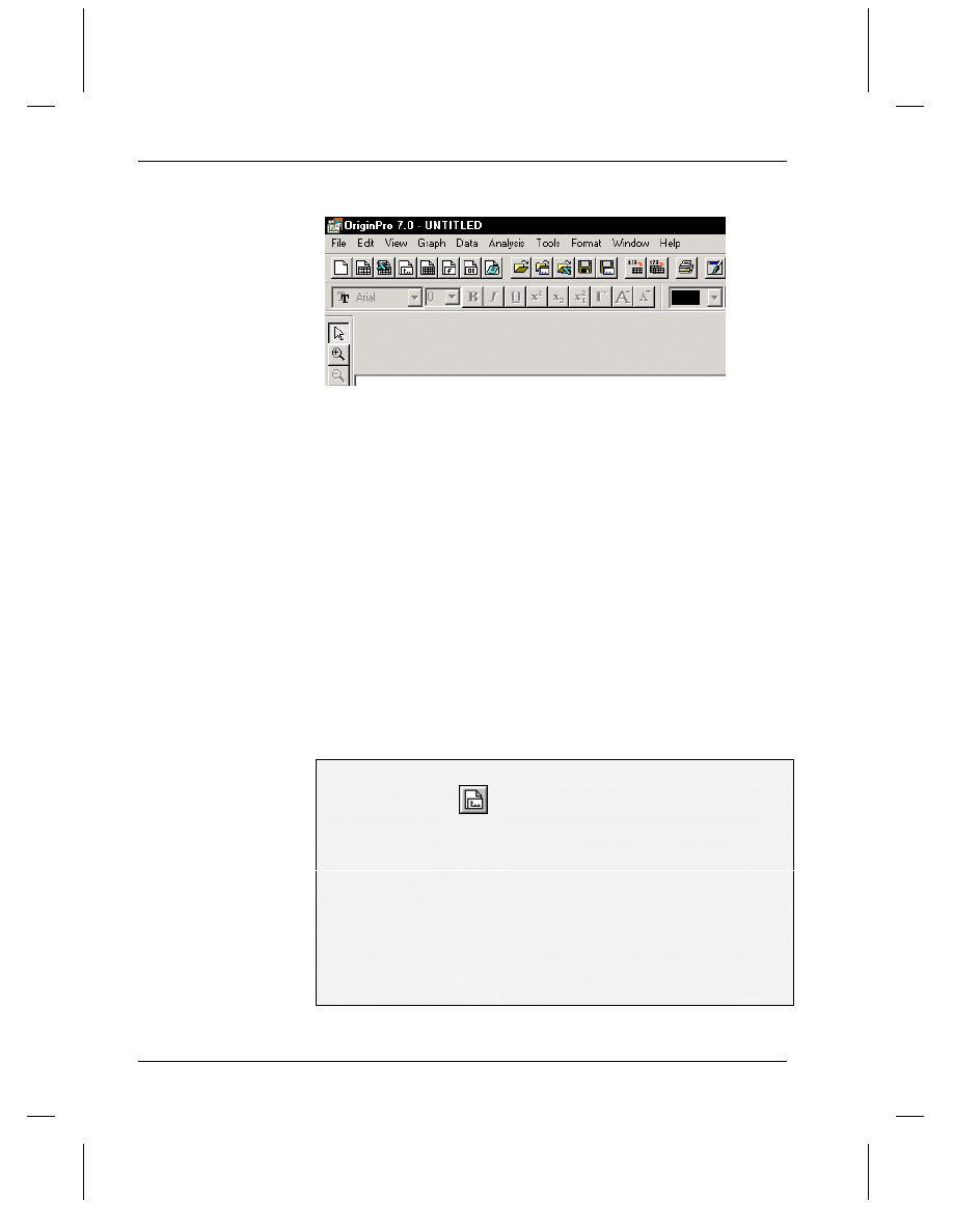
Tutorial 7, Working with Excel in Origin

196

•

Plotting an Excel Workbook in Origin

Figure 6: The Toolbar Spacer

Creating a Data Plot by Dragging Data Into a
Graph

When you drag Excel workbook data into a graph, Origin makes
assumptions about the plotting designations of the selected data.
=> If one column (or a range from one column) is highlighted, then this
column supplies the Y values for the data plot. The data is plotted versus
row number.
=> If more than one column (or a range from more than one column) is
highlighted, the leftmost column supplies the X values. All other
columns supply the Y values. The data is plotted versus the X values.
=> If more than one column (or range from more than one column) is
highlighted and the CTRL key is depressed while dragging the data, then
all the columns supply the Y values. The data is plotted versus row
number.

To Create a Graph Using the Drag-and-Drop Method:

1) Click New Graph

on the Standard toolbar. Move the new

Graph2 window to the lower-right corner of the workspace, so that when
the workbook is active it won’t completely overlap the new graph
window.
2) Select Window:Book1 to activate the Excel workbook window.
3) Highlight the first two columns in the workbook.
4) Click on the right edge of the selected workbook data, then drag the
data to the Graph2 window. When you release the mouse button, column
B is plotted against column A as a line plot in the graph window.
5) Click on the graph window to make it the active window.

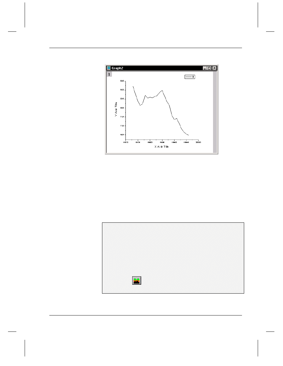
Tutorial 7, Working with Excel in Origin

Plotting an Excel Workbook in Origin

•

197

Figure 7: Dragging Data into a Graph Window

Creating a Graph Using Origin’s Default Plot
Assignments

For a complete
discussion on this
feature, see the Origin
Help.

This plotting method allows you to select your workbook data and graph
type, and then Origin creates the data plots by making assumptions
about the plotting assignments of the selected data. This plotting
method is not available by default. It must be activated from the
Options dialog box.

To Create a Graph Using the Default Plot Assignments:
1) Select Tools:Options to open the Options dialog box. (If the
workbook is active, then select Window:Origin Options.)
2) On the Excel tab, select the Default Plot Assignments check box.
3) Click OK, then click No in the dialog box that opens.
4) Make the Excel workbook active.
5) Click on the column A heading, then CTRL+click on the column D
and G headings.

6) Click Area

on the 2D Graphs toolbar.

7) Reposition the legend so that the entire legend is on the graph page.

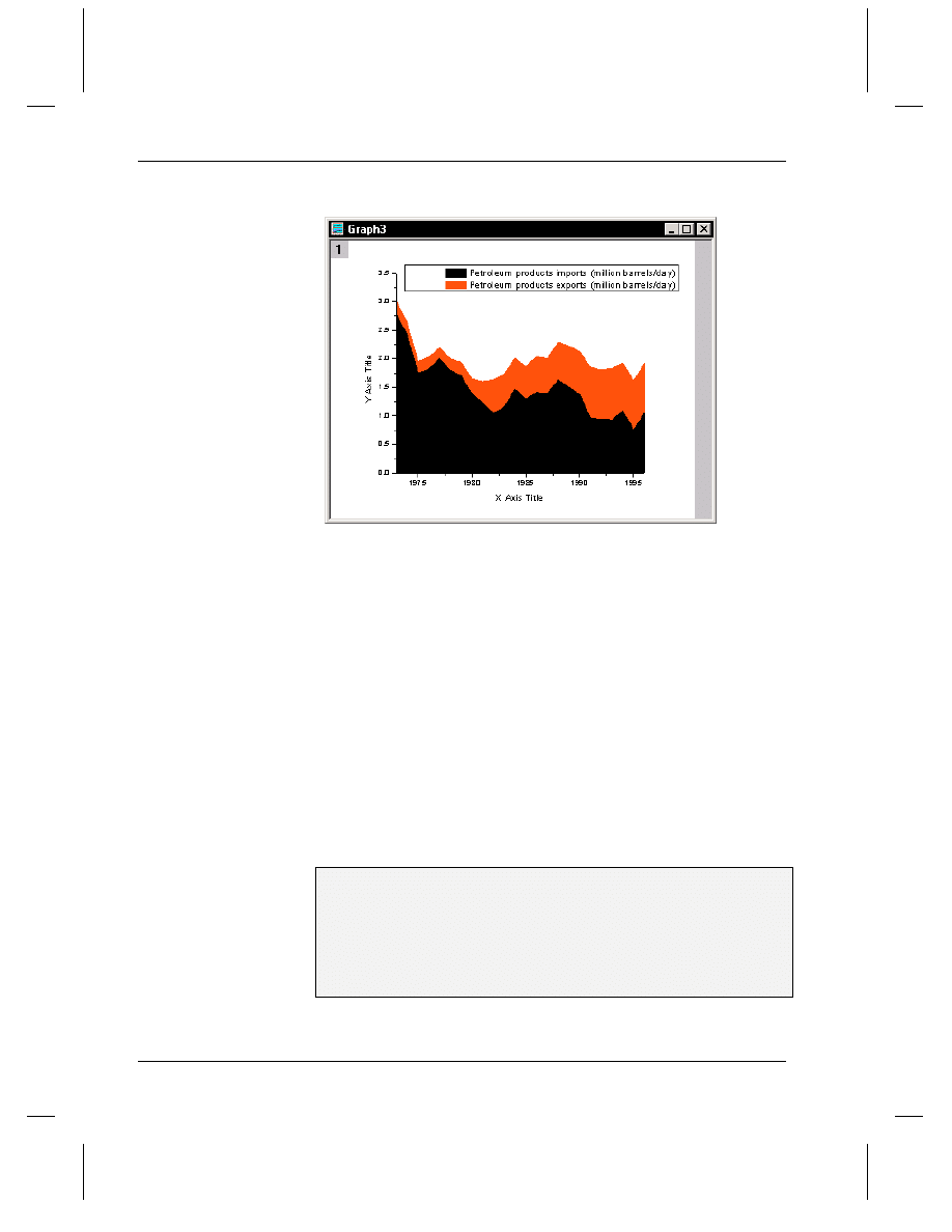
Tutorial 7, Working with Excel in Origin

198

•

Saving an Excel Workbook in Origin

Figure 8: Plotting Excel Data Using the Default Plot Assignments

Saving an Excel Workbook in Origin

There are two ways to save Excel workbooks in Origin projects. You
can save the workbook internal or external to the Origin project. When
you save a workbook internal to the project, it is saved as part of the
Origin project and can only be opened by opening the project. When you
save a workbook external to the project, a link to the workbook is saved
within the Origin project and the workbook can be opened and edited
with Excel.
By default, pre-existing workbooks that are opened in an Origin project
are saved external to the project, whereas workbooks that are created
from within Origin are saved internal to the project. However, the save
option can be changed in the Workbook Properties dialog box.

To Save the Workbook Internal to the Origin Project:
1) Make the Excel workbook active.
2) Right-click on the title bar of the workbook and select Properties
from the shortcut menu. This opens the Workbook Properties dialog
box.
3) Select the Internal radio button in the Save As group.

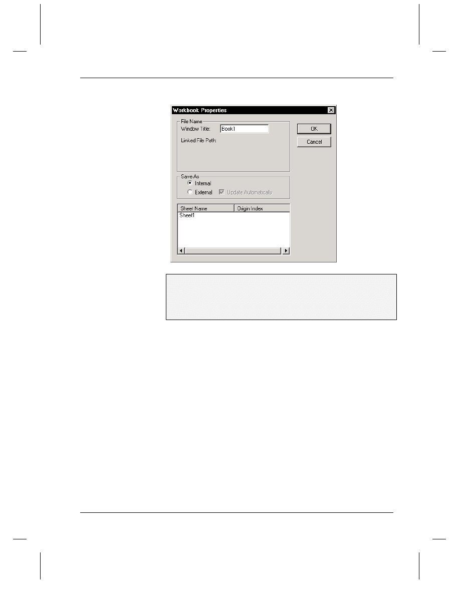
Tutorial 7, Working with Excel in Origin

Saving an Excel Workbook in Origin

•

199

Figure 9: The Workbook Properties Dialog Box

4) Click OK.
5) Select File:Save Project As.
6) Type Excel_Tutorial in the File Name text box.
7) Click Save.

The project is saved and the workbook is saved internal to the project.
Any changes that you now make to the Excel workbook located in the
\TUTORIAL folder will not be reflected in the project file the next time
it is opened.

Tutorial 7, Working with Excel in Origin

200

•

Saving an Excel Workbook in Origin

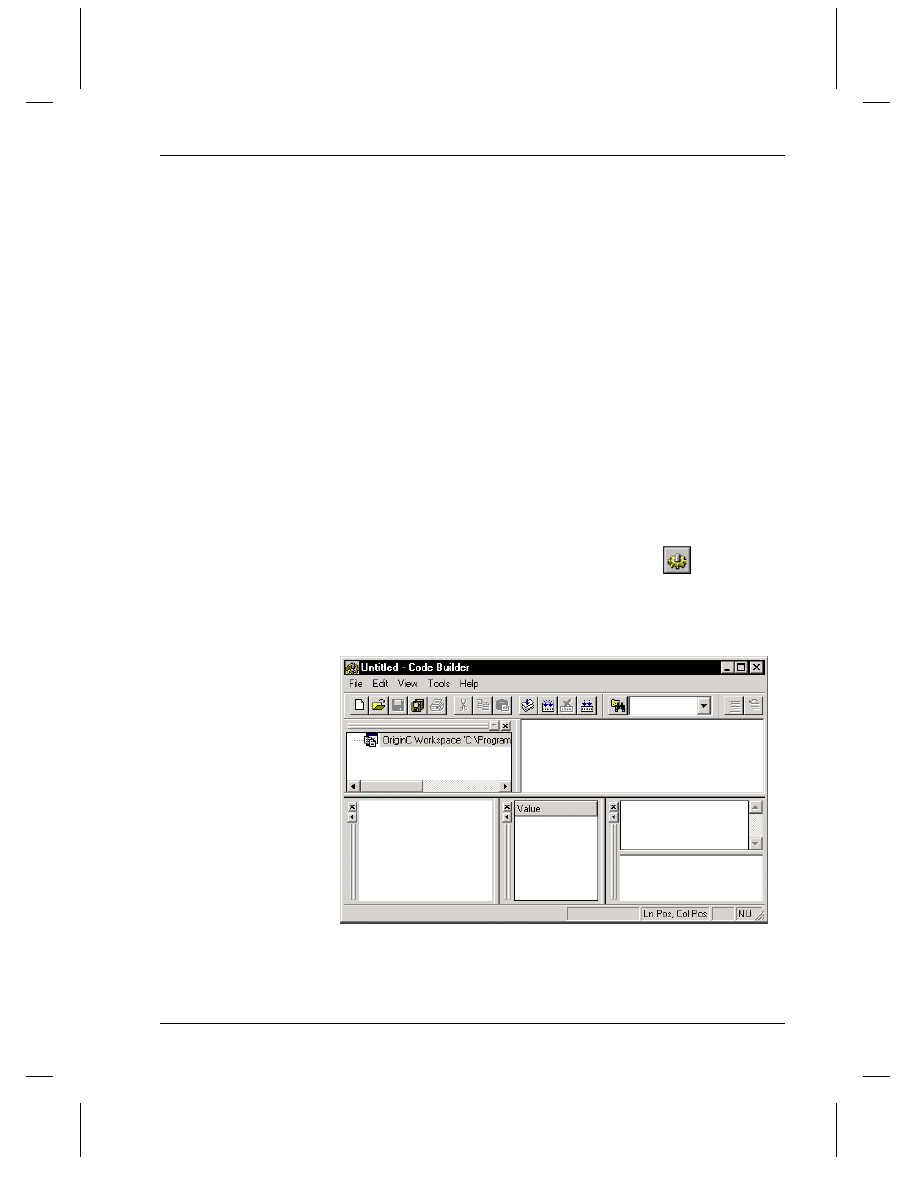
Tutorial 8, Programming in Origin

Introduction

•

201

Tutorial 8, Programming in

Origin

Introduction

Origin's programming language is called Origin C. Origin C supports a
nearly complete ANSI C language syntax as well as a subset of C++
features including internal and DLL-extended classes. In addition,
Origin C is "Origin aware". This means that Origin objects such as
worksheets and graphs are mapped to classes in Origin C, allowing direct
manipulation of these objects and their properties from Origin C.
Origin C's integrated development environment is called Code Builder.

To open Code Builder, click the Code Builder button

on the

Standard toolbar.

Figure 1: Code Builder

LabTalk Console

Variables

Output

Workspace

Multiple Document Interface (MDI)

Code Builder provides tools for writing, compiling, and debugging your
Origin C functions. Once an Origin C function is compiled, the function
becomes available from Origin.

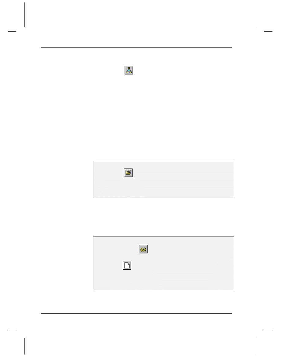
Tutorial 8, Programming in Origin

202

•

Creating a New Source File

For more information,
review the Programming
Guide and the sample
projects and source files
located in the Origin
\Samples\Programming\
subfolders.

A number of techniques are available to call your compiled Origin C
functions from Origin. For example, you can program the Custom

Routine button

located on Origin's Standard toolbar. You can also

program objects on windows, create new toolbar buttons, and even
create new menu commands. Additionally, Origin C functions can be
called from a number of Origin dialog boxes, including the nonlinear
curve fitter and the Set Column Values dialog box.
This tutorial will show you how to create, compile, and test an Origin C
function. You will then learn how to call your Origin C function from
Origin. In this example, you will call the function to set a column's
values.

Creating a New Source File

The data for this tutorial lesson is provided in an Origin project file.

To Open the Project File:

1) Click Open

on the Standard toolbar.

2) In the Origin \TUTORIAL folder, select TUTORIAL_8.OPJ from the
list of files.
3) Click Open.

A project opens displaying a notes window and a worksheet window.
The notes window contains the function that you will compile. (This is
provided so that you don't have to re-type the function.)
To create a new function for global use in Origin, you must first open
Code Builder.

To Open Code Builder and Create a New Source File:

1) Click Code Builder

on Origin's Standard toolbar. Code Builder

opens displaying a default workspace.

2) Click New

on Code Builder's Standard toolbar. This opens the

New File dialog box.
3) If C File is not selected in the top list box, then select it.
4) In the File Name text box, type MyFunction.

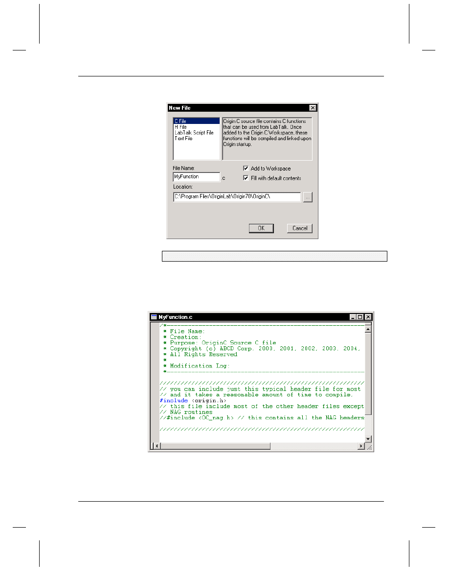
Tutorial 8, Programming in Origin

Creating a New Source File

•

203

Figure 2: Creating a New Source File

5) Click OK.

A new source file window opens in Code Builder's Multiple Document
Interface (MDI).

Figure 3: The Source File Window

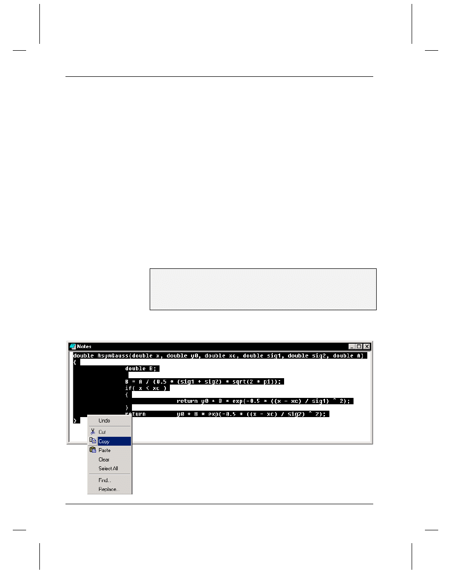
Tutorial 8, Programming in Origin

204

•

Coding Your Function

When Code Builder creates a new source file, it adds starting contents to
the source file. (This is the default setting in the New File dialog box.)
This starting contents includes comments and one

#include

preprocessor directive:

#include <origin.h>

Origin 7 includes a
number of the NAG
function libraries. These
functions are referenced
in the Origin C
Reference Help.

The origin.h header file contains

#include

preprocessor directives for

all the additional Origin C header files except for the NAG header files.
(Note: To open the origin.h header file in the MDI, right-click on the
text "origin.h" in the

#include

preprocessor directive of your new

source file and then select Open "origin.h" from the shortcut menu.
You can open any included file using this method as long as the

#include

preprocessor directive is not commented out.)

As with the C programming language, your Origin C function definitions
must include a function header and a function body. The Origin C
function definition for this example is provided in the Origin notes
window.

To Enter the Function Definition:
1) Make Origin the active program.
2) From the notes window, copy the entire function definition for

AsymGauss

into the Clipboard.

Figure 4: Copying the AsymGauss Function to the Clipboard

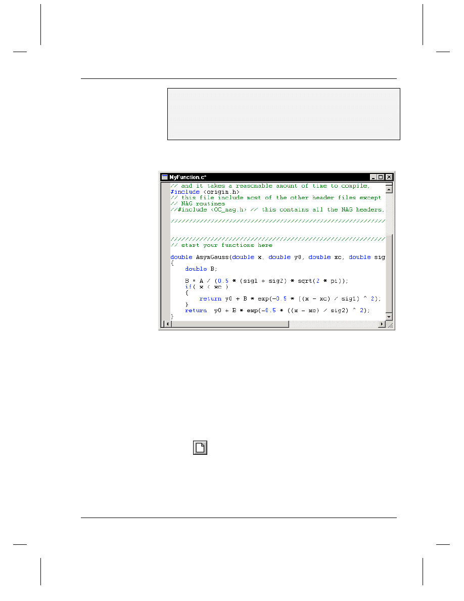
Tutorial 8, Programming in Origin

Compiling and Testing the Function

•

205

3) Make Code Builder the active program.
4) In the source file window, click after the line that reads

// start

your functions here

5) Paste the

AsymGauss

function definition into the source file

window.

Figure 5: Pasting the AsymGauss Function into the Source File Window

To make your code easier to read and edit, the Code Builder text editor
automatically displays different elements of your code using different
colors. Additionally, the text editor automatically indents your text
depending on the previous lines of code.

Compiling and Testing the Function

Only source files that have been added to the Code Builder workspace
can be compiled. When you create a source file by clicking the New

button

or by selecting File:New, the source file is added to the

workspace by default. However, if you open an existing source file you
must select the Add to Workspace check box in the Open dialog box to
add the file to the workspace. If you don't select this check box when
opening a source file, you can add the file to the workspace later by

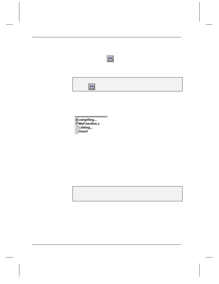
Tutorial 8, Programming in Origin

206

•

Compiling and Testing the Function

selecting File:Add to Workspace when the source file is active in the
MDI.
To compile and link the functions that have been added to the workspace,

click the Build button

on the Standard toolbar. If you encounter a

compile error in the Output window, double-click on the error line to
activate the source file and show the error line.

To Build the AsymGauss Function:

1) Click

on Code Builder's Standard toolbar.

Your function is compiled and linking is performed. The compilation
results are output to the Output window.

Figure 6: Successfully Building the AsymGauss Function

To test your compiled function in Code Builder, you can call the function
from the top pane of Code Builder's LabTalk Console.

To learn more about
LabTalk, review the
LabTalk Reference Help.

LabTalk is Origin's historical programming language. LabTalk scripts
are interpreted during execution by Origin, whereas Origin C code is
compiled to byte code form and therefore executes much faster than
LabTalk. Because of this, most of your Origin programming should be
done in Origin C functions. However, you must still use LabTalk to call
your Origin C functions from Origin.

To Test the AsymGauss Function:
1) Click in the top pane of Code Builder's LabTalk Console. The
console is located in the lower-right corner of Code Builder.

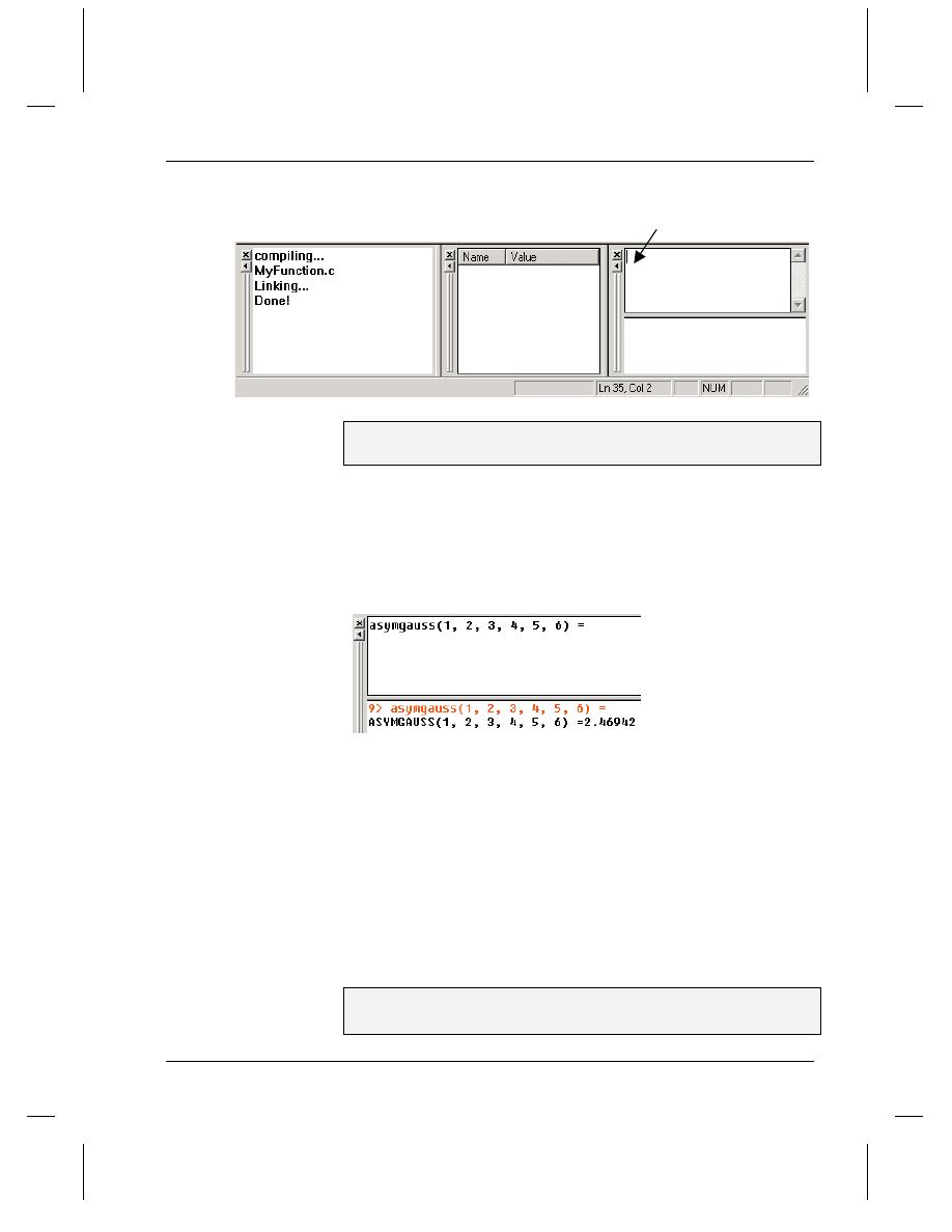
Tutorial 8, Programming in Origin

Using the Function in Origin

•

207

Figure 7: The LabTalk Console

Click here.

2) Type the following text and then press ENTER:

asymgauss(1, 2, 3, 4, 5, 6) =

(Note that a LabTalk call to an Origin C function is not case-sensitive.
However, Origin C is case-sensitive.)
You should see the following result in the bottom pane of the LabTalk
Console (except your line number will be different).

Figure 8: Testing the AsymGauss Function in the LabTalk Console

The

AsymGauss

function is ready to use in Origin.

Using the Function in Origin

After you compile an Origin C function, you can call the function from
Origin. For example, you can call the function from the Script window,
from the Label Control dialog box of an object, or from any other
LabTalk script location. You can also call your function from the
nonlinear curve fitter and from the Set Column Values dialog box.

To Set a Column's Values using the AsymGauss Function:
1) Make Origin the active program.

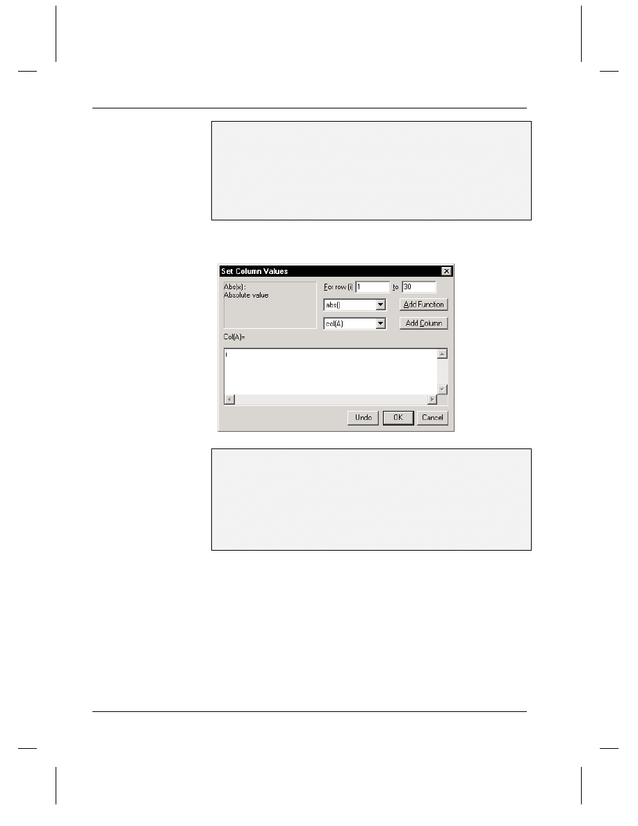
Tutorial 8, Programming in Origin

208

•

Using the Function in Origin

2) Activate the Data1 worksheet.
3) Click the A column heading to select the column.
4) Select Column:Set Column Values. This opens the Set Column
Values dialog box.
5) In the Col(A) = text box, replace the highlighted text with i. This
instructs Origin to fill rows one through 30 in column A with row
numbers.

Figure 9: Setting the Column A Values

6) Click OK.
7) Click the B column heading to select the column.
8) Select Column:Set Column Values. This re-opens the Set Column
Values dialog box but for column B.
9) In the Col(A) = text box, replace the highlighted text with the
following:

asymgauss(col(a), 2, 3, 4, 5, 6)

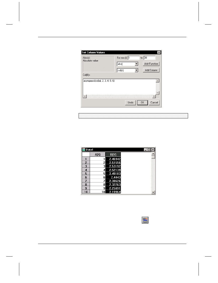
Tutorial 8, Programming in Origin

Using the Function in Origin

•

209

Figure 10: Setting the Column B Values

10) Click OK.

For every cell in column B rows one through 30, Origin calls the

AsymGauss

function and passes it the associated value in column A as

the first argument, and 2, 3, 4, 5, and 6 as the remaining arguments.

Figure 11: The Updated Worksheet

Note: The values in column B are calculated from the values in column
A, as defined by the

AsymGauss

function. If the values in column A

are changed, the column B values will not update automatically. To
update the values in column B, select Analysis:Set All Column Values

or click the Set All Column Values button

on the Worksheet Data

toolbar.

Tutorial 8, Programming in Origin

210

•

Using the Function in Origin

Index

•

211

Index

2D binning

worksheet to matrix conversion

163

2D graphs

plotting introduction 90
toolbars 51

3D surface graphs

adding contours 172
changing colormap levels 168
creating 166
rotating 173

Analysis

ANOVA 39
data coordinates 99
fitting 141
normality test 41
range of data 101
results of

Results Log 67

survival 38
t-Tests 37

ANOVA 39
Appending

projects 74

Arrows and lines

adding to graphs 23

ASCII

importing 87

Axes

adding a layer 129, 131
customizing 93

linking layers 134

Categorical data 30
Circles

adding to graphs 23

Code Builder See also Origin C

adding file to workspace 206
building workspace 206
creating a new source file 202
introduction 201
LabTalk Console 206
opening 202
programming 42, 69

Color images

importing 33

Color map

changing colors

individual color 171
range 170

changing levels 168

Columns

multiple X 127
setting designation 89
setting values 109
sorting 110

Computers

minumum configuration needed 7

Coordinates of data point 99
Cox Proportional Hazards Model 38
Customizing

ASCII import options 87
axes 93
data plot color 130
graphs 93
templates 82

Data plots

adding to layer 130
changing color 130
determining if different 42, 144
fitting 115
masking data 106, 114
removing from layer 156
selecting a range 101

Data points

masking 106, 114
reading value 99

Data Reader tool 99
Data Selector tool 101

Index

212

•

Index

D Continued

Data sets

determining if different 42, 144
setting values 109
sorting 110

Designating

multiple X columns 127

Development environment

Code Builder 42, 69

Drag-and-drop

Excel data into graph 196
importing data 29, 86

Drawing objects

adding to graphs 23

Enlarger tool 91, 102
Error bars

designating columns as 89

Excel See also Windows

menu bar 61
opening workbooks 191
plotting data 193, 194, 196, 197
saving with project 198
toolbar spacer 61, 195

Explorer See Project Explorer
Exporting

format options 189
layout pages 187
size of picture 188

File tracking 74
Finding

windows in project 66

Fit Comparison tool 42, 144
Fitting See also NLSF

advanced fitting tool 146
from the menu 115
linear 115
two data sets to same function 42,

144

using the menu commands 141
using the tools 143
wizard 26, 145

Folder See Project Explorer
Freehand object

adding to graphs 23

F-Test

Fit Comparison tool 42, 144

Full menu 47

Graphic images

importing 33

Graphs See also Windows

adding a layer 129, 131
adding data to 130
adding drawn objects 23
adding text 21, 95
categorical data 30
creating 57
customizing 93
introduction 57
layers 121
magnifying 102
menu bar 58
plotting from worksheet 90
reading data point value 99
removing data from 156
saving as templates 140
selecting a range of data 101
templates 81
zooming in or out 104

Gray scale images

importing 33

Gridding

worksheet to matrix conversion

164

Histograms

raster graphic images 35

Image graphs 33

region of interest 51, 105

Image histograms 35
Importing

ASCII 87
drag-and-drop 29
raster graphic images 33
supported formats 85
Thermo Galactic SPC 28

Installing Origin 7
Integrated development environment

See Code Builder

Index

•

213

Kaplan-Meier Product Limit

Estimator 38

LabTalk Script window 70
Launching Origin 17
Layer tool 129
Layers

activating 122
adding 129, 131
adding data to 130
arranging 131
introduction 121
linking axes scales 134
removing data 156

Layout pages See also Windows

adding pictures 178
adding text 181
arranging pictures and text 182
creating 177
exporting 187
introduction 59
menu bar 60
rotating 178

Legends

customizing 136

Linear Fit tool 143
Lines and arrows

adding to graphs 23

Linking

layers 134

Magnifying data 91, 102, 104
Masking

single data point 106, 114

Matrices See also Windows

converting from worksheets 163
introduction 159
mapping the XY coordinates 159
menu bar 62, 63
plotting 161, 166
setting dimensions 159
setting values with a function 160
showing XY values 160

full and short 47
introduction 46

NAG

function libraries in Origin 43

NLSF

advanced fitting tool 146
assigning variables to data sets 150
calculating reduced chi-square 154
closing 155
creating results worksheet 155
defining a function 149
initializing parameters 152
Levenberg-Marquardt iterations

154

simulating curves 152
wizard 26, 145

Nonlinear curve fitting See NLSF
Normality test 41
Notes

menu bar 64

Object Edit toolbar

arranging pictures on layout 182

Opening

Excel workbooks 191
existing project 74, 123
new project 72
windows from a file 79

Origin

Help files 2
installing 7
manuals 2
registering 17
starting 17
technical support 2
un-installing 13, 14, 17

Origin C See also Code Builder

compiling functions 206
defining a function 204
programming 42, 69
testing functions 206
using functions in Origin 207

OriginLab

additional products

add-on modules 5
OriginPro 3
Peak Fitting Module 4

web site 2

OriginPro

overview of 3

Index

214

•

Index

Peak Fitting Module

overview of 4

Performance

hiding toolbar spacer 48
optimizing workspace view

Project Explorer 65

Plotting

Excel data 193, 194, 196, 197
matrix data 166
ranges of worksheet data 113
worksheet data 90

Polygons

adding to graphs 23

Polynomial Fit tool 143
Programming See Origin C
Project Explorer

closing and opening 66
controlling workspace view 65
creating folders 65
description 64
searching for windows 66

Projects

appending multiple 74
backups 72
creating new 72
opening 74, 123
organizing 64
saving 71, 97
tracking paths 74

Raster graphic images

importing 33

Rectangles

adding to graphs 23

Region of data 91, 101, 102, 104
Region of interest

image 51, 105

Registering Origin 17
Results Log 67
Rotating

3D surface graphs 173
layout pages 178

Saving

Excel workbooks with project 198
projects 71, 97
templates 140

windows to a file 78

Scale See Axes
Screen location

reading value 100

Screen Reader tool 100
Script window 70
Searching

windows in project 66

Shapiro-Wilk

normality test 41

Short menu 47
Sigmoidal Fit tool 143
Sorting

worksheet data 110

SPC files

importing 28

Speed

optimizing workspace view

Project Explorer 65

Speed mode 166
Starting Origin 17
Statistics

ANOVA 39
normality test 41
survival analysis 38
t-Tests 37

Survival analysis 38
System requirements 7

Technical support 2
Templates

creating windows 81
customizing 82
graphs 81
saving graphs as 140

Text

adding to graphs 21, 95
adding to layout pages 181
legends 136

Thermo Galactic SPC

importing 28

Toolbar spacer

hiding 195

Toolbars

2D Graphs 51
2D Graphs Extended 52
3D Graphs 52
3D Rotation 52
Arrow 54
Column 53
creating new 54

Index

•

215

T Continued

customizing default 54
Edit 51
Format 50
Graph 49
introduction 48
Layout 53
Mask 53
Object Edit 53
spacer 48
Standard 49
Style 50
Tools 50
Worksheet Data 52

Tools

Enlarger 91, 102
fitting 143
Zoom In 104
Zoom Out 104

Tracking

files 74

t-Tests 37

Un-installing Origin 13, 14, 17
Upgrading Origin 7

Viewing modes

workspace

controlling with Project Explorer

Web site

OriginLab 2

Windows See also Templates

controlling view with Project

Explorer 65

creating new 75
deleting 77
duplicating 78
finding in project

Project Explorer 66

hiding 77
opening existing 79
refreshing 78
renaming 76
saving 78

templates 81

Worksheets See also Windows

column plotting designations 55
converting to matrices 163
introduction 55
menu bar 56
multiple X columns 127
plotting range 113
setting column values 109
setting display range 112
sorting 110

Workspace

closing Project Explorer 66
controlling view with Project

Explorer 65

Zoom tool 104

Document Outline

Introduction
Installing and Registering Origin
- Chapter 2, Installing and Registering Origin
What's New in Version 7
- Chapter 3, What's New in Version 7
Getting Started Using Origin
- Chapter 4, Getting Started Using Origin
Tutorial 1, Plotting Your Data
- Tutorial 1, Plotting Your Data
Tutorial 2, Exploring Your Data
- Tutorial 2, Exploring Your Data
Tutorial 3, Creating Multiple Layer Graphs
- Tutorial 3, Creating Multiple Layer Graphs
Tutorial 4, Nonlinear Curve Fitting
- Tutorial 4, Nonlinear Curve Fitting
Tutorial 5, Creating 3D Surface Graphs
- Tutorial 5, Creating 3D Surface Graphs
Tutorial 6, Creating Presentations with the Layout Page
- Tutorial 6, Creating Presentations with the Layout Page
Tutorial 7, Working with Excel in Origin
- Tutorial 7, Working with Excel in Origin
Tutorial 8, Programming in Origin
- Tutorial 8, Programming in Origin

Wyszukiwarka

Podobne podstrony:
Neuro Solutions 5 Getting Started Manual
Getting Started
getting started IAOTAGZXANHHC6G Nieznany
(ebook pdf) Matlab Getting started
Part I Getting Started
1 3 Getting started with Data Studio Lab
Getting Started with PostHASTE
Packt Publishing Getting Started with Backbone Marionette (2014)
Getting Started
ANSYS Getting Started Tutorial Workbench
chinas southwest 3 getting started
1 2 Getting started (2)
mr zr getting started
Matlab Getting Started
01 GETTING STARTED
Part I Getting Started

więcej podobnych podstron

GETTING STARTED MANUAL

Document Outline