Theoretical Information About Branch-line Couplers

Generally branch-line couplers are 3dB, four ports directional couplers having a 90

°

phase

difference between its two output ports named through and coupled arms. Branch-line couplers

(also named as Quadrature Hybrid) are often made in microstrip or stripline form.

1.DESIGN OF BRANCH -LINE COUPLER:

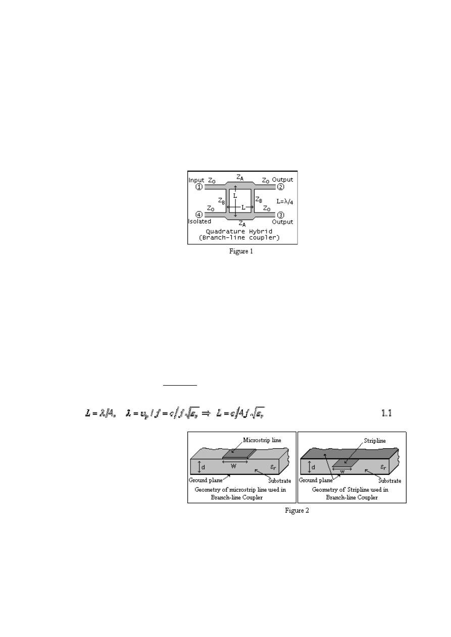
The geometry of the branch-line coupler is shown in Figure1. A branch-line coupler is

made by two main transmission lines shunt-connected by two secondary (branch lines). As it can be

seen from the figure, it has a symmetrical four port. First port is named as Input port, second and

third ports are Output ports and the fourth port is the Isolated port. The second port is also named

as direct or through port and the third port is named as coupled port. It is obvious that due to the

symmetry of the coupler any of these ports can be used as the input port but at that time the

output ports and isolated port changes accordingly. When we analysis the scattering matrix of this

coupler we will see also the result of that symmetry in scattering matrix.

Considering the dimensions of the coupler the length of the branch line and series line is

generally chosen as the one fourth of the design wavelength . As it is shown in Figure 1, if we

name the length of series and stub transmission lines as L then L can be find as following:

At that point we will se the calculation of the other dimension parameter of transmission

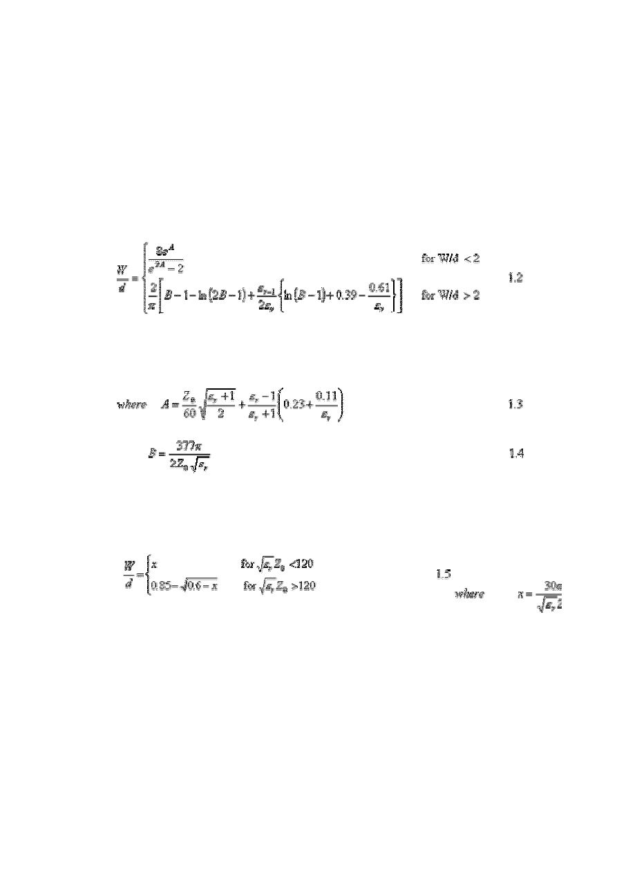
lines; w/d ratio. We generally design branch-line couplers in two forms: Microstrip line and Stripline.

Geometry of the microstrip line and stripline can be seen from Figure2.

According to the impedance choice of the series and stub microstrip transmission lines we

can calculate the w/d ratios of the those lines in microstrip form by using the following formulas:

Given

ε

r

and Z

0

Considering the Stripline branch-line coupler design, we can calculate w/d ratios for each

(stub and series) transmission line in the branch-line coupler with following calculations:

2.ANALYSIS OF BRANCH-LINE COUPLER

2.1.Even-odd mode analysis and S-parameters

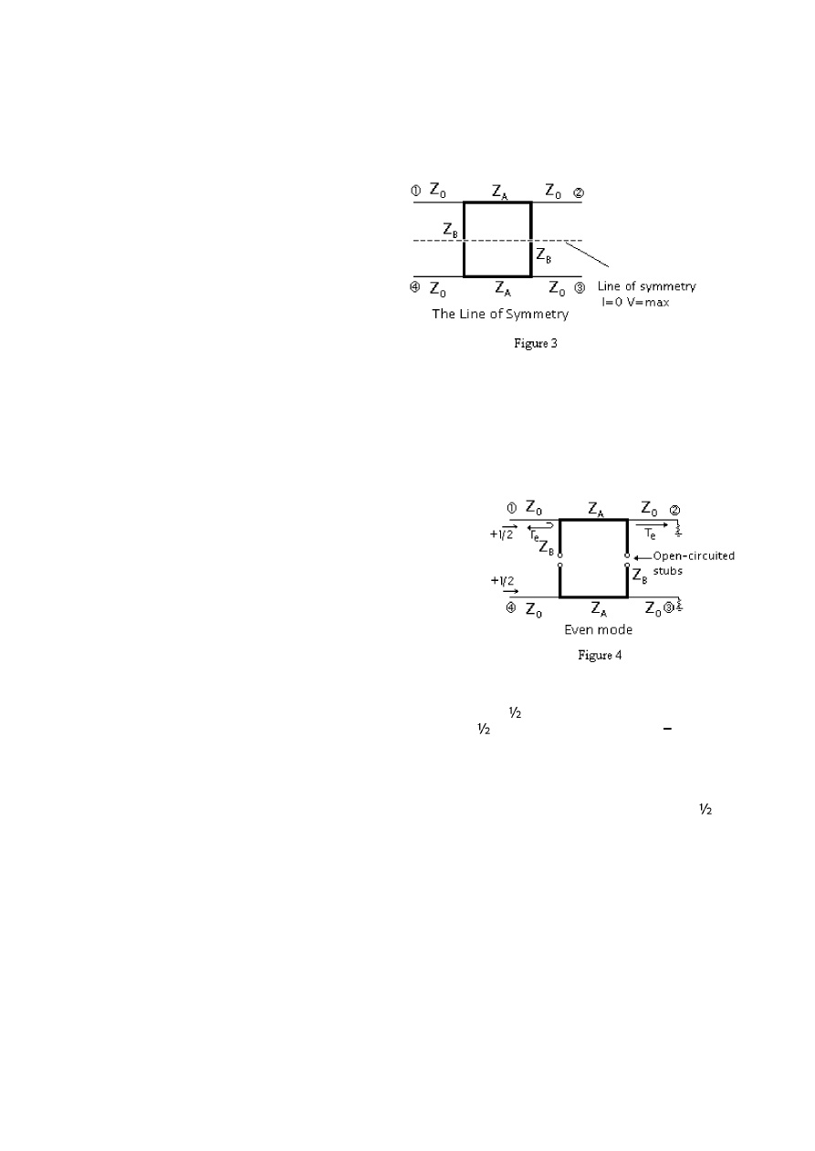
In the analysis of the branch-line coupler we consider the scattering matrix of the coupler.

In order to find them we use even-odd .mode analysis. In both mode we divide the branch-line
coupler symmetrically as in the Figure 3.

Generally considering that we give V voltage to the Input port. In the even odd mode

analysis we consider it we give that V voltage in even mode

of it to Input port and rest to the

Isolated port and for the odd mode we give Input port of it and to the isolated port 1/2 of it.

Furthermore, while making even-odd mode analysis, for the even mode we think that the stubs of

the divided circuit are open circuited and for the odd mode they are short circuited. For this

analysis, if we consider the superposition of the incoming voltage, it results as V voltage to the

Input and 0 voltage to the Isolated port. Furthermore we have for each mode incident and reflected

waves, for even mode it is illustrated in the Figure 4. As it is seen we have an incident wave of

the actual voltage and at first stub we have a reflection having a reflection coefficient

Γ

e and at

second port a transmitted signal having transmission coefficient Te. Considering the contribution of

the even mode to the port waves for first port we have 1/2V

Γ

e, for second port we have 1/2VTe,

for third port 1/2VTe, and for the fourth port 1/2V

Γ

e.

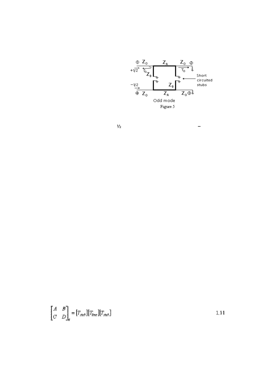
In addition, for odd mode incident and reflected waves are illustrated in the Figure 5. As it

is seen we have an incident wave of the actual voltage at first port and

1/2 of it at fourth port

as incoming wave. Also at first stub we have a reflection having a reflection coefficient

Γ

o and at

second port a transmitted signal having transmission coefficient To. Considering the contribution of
the odd mode to the port waves for first port we have 1/2V

Γ

o, for second port we have 1/2VTo, for

third port -1/2VTo, and for the fourth port --1/2V

Γ

o. At this point, we express the emerging wave

at each port of the branch-line coupler as the superposition of the even and odd mode waves as

following:

B

1

=(1/2

Γ

e+1/2

Γ

o)V

1.7

B

2

=(1/2Te+1/2To)V

1.8

B

3

=(1/2Te-1/2To)V

1.9

B

4

=(1/2

Γ

e-1/2

Γ

o)V

1.10

The ABCD matrix is used to find the overall transmission and reflection characteristics of

the network. Having Y

A

=1/Z

A

and Y

B

=1/Z

B

we have the ABCD matrix of even and odd mode. For

even mode ABCD parameters are as following:

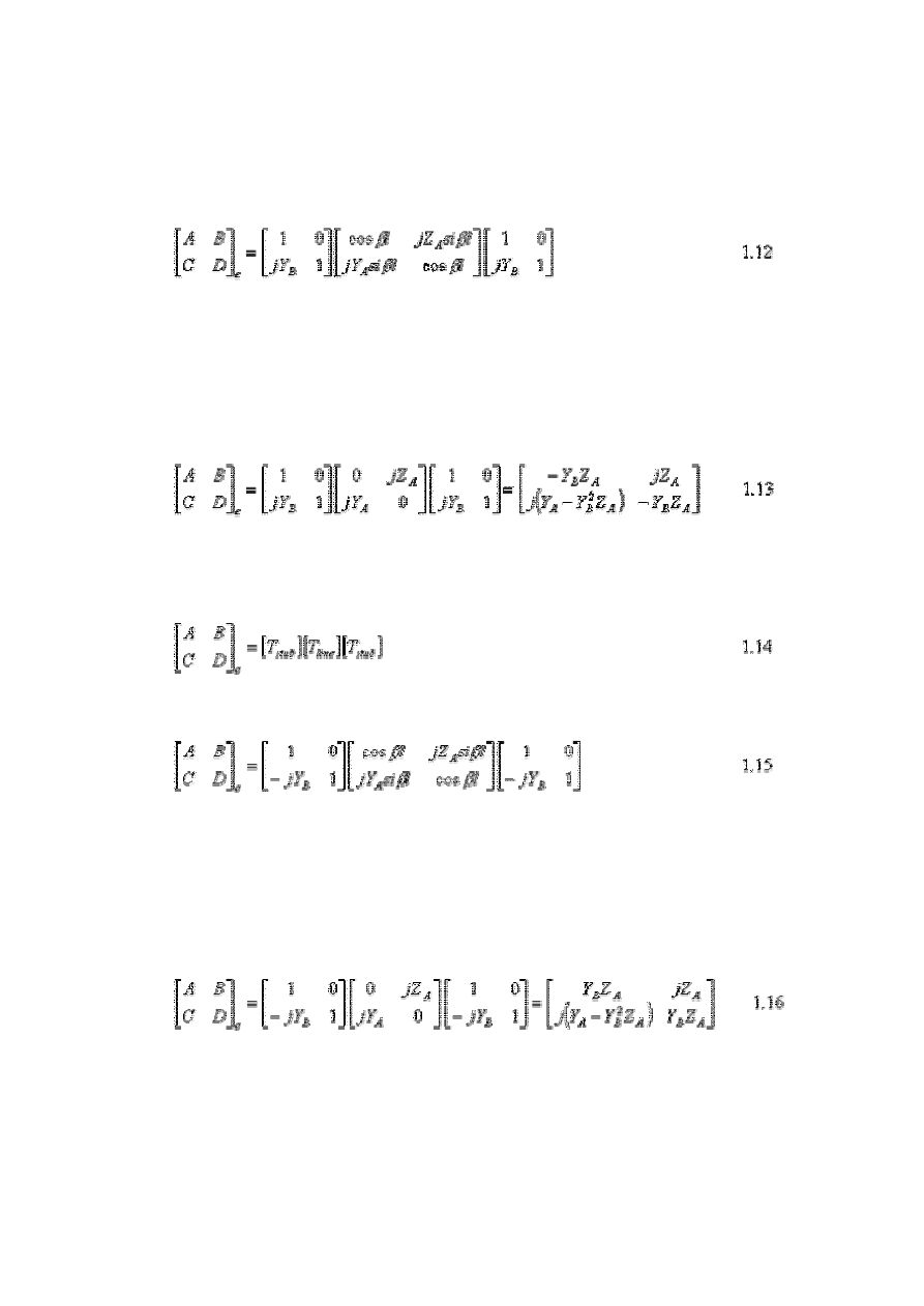
Since we have l=

λ

/4 (and work with our design frequency),

β

l=(2

π

/

λ

)*(

λ

/4)=

π

/2

Therefore cos

β

l=0 and sin

β

l=1 and the ABCD matrix is following:

For the odd mode ABCD matrix:

Since we have l=

λ

/4 and so

β

l=(2

π

/

λ

)*(

λ

/4)=

π

/2

So cos

β

l=0 and sin

β

l=1 and the ABCD matrix is following

At that point we can find

Γ

e,

Γ

o, Te, To by using following equations:

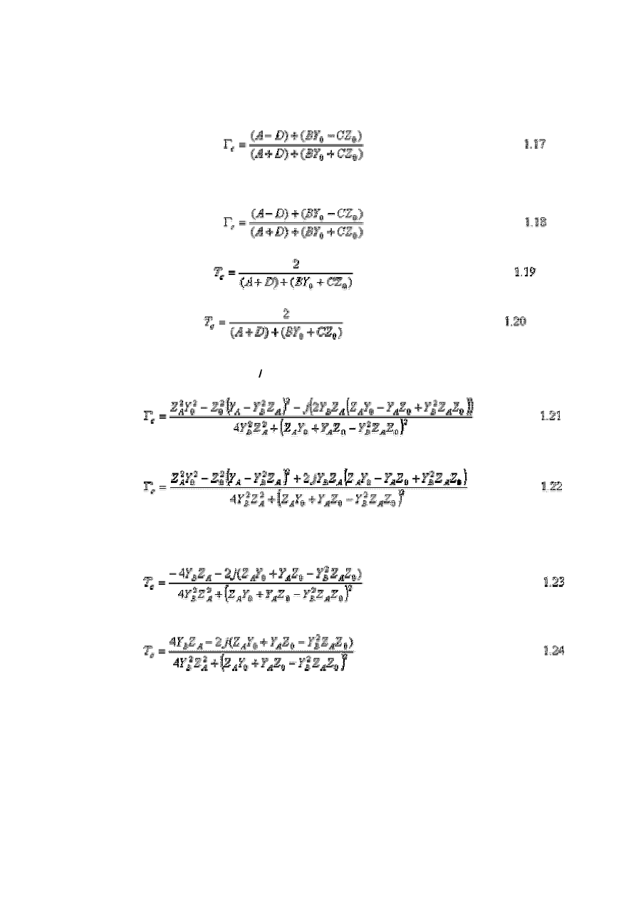
Then solving above equations with parameters of even and odd mode ABCD matrixes at center

frequency where

ƒ

=

ν

p

/

λ

=

ν

p

/4 :

At this time we can say that B

1

/V=S

11

, B

2

/V=S

12

, B

3

/V =S

13

and B

4

/V =S

14.

Therefore S-

Parameters are as following:

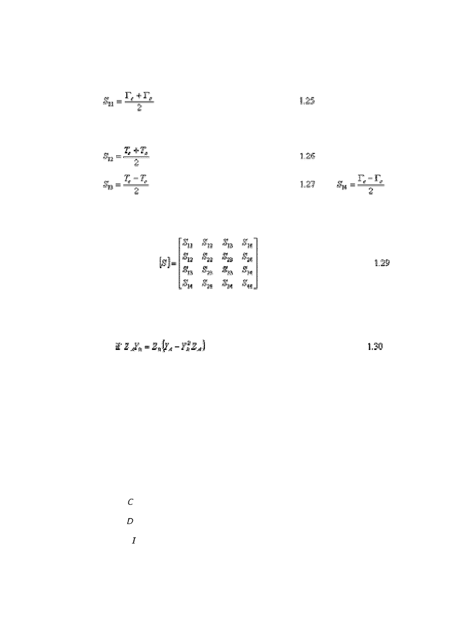
And the scattering matrix of

Branch-line coupler is

2.2. Matching Condition

Looking above equations if we consider the matching condition;

then

S

11

and

S

14

becomes zero. In that matching case; the power entering port1is evenly divided between ports

2 and 3 with a 90

°

phase shift between these output ports. No power is coupled to port 4 (isolated

port). Therefore, the isolation and directivity of that matched coupler, which will be mentioned in

following part, is very high (for perfect case infinity), at center frequency.

2.3.Coupling, Directivity, Isolation and Power-split Ratio

As it can be seen from the matrix above that scattering matrix of branch-line coupler is

symmetric and the each row of it is just the transpose of its each column.

Considering the coupling which is the ratio of power at port 1 to power at port 3, directivity which is

the ratio of power at port 3 to power at port 4 and the isolation which is the ratio of power at port

1 to power at port 4 of the branch-line coupler:

Coupling = = 10log(P

1

/P

3

) = -20log |S

13

| dB

1.31

Directivity = = 10log(P

3

/P

4

) = 20log (|S

13

|/|S

14

|) dB 1.32

Isolation = = 10log(P

1

/P

4

) = -20log|S

14

| dB

1.33

The power split ratio (P) which is used to express the coupling of the branch-line coupler in

terms of the ratio of powers to the coupled (port 3) and direct ports (port 2) :

= 10log(P

3

/P

2

)=-20log (|S

13

|/|S

12

|)

1.34

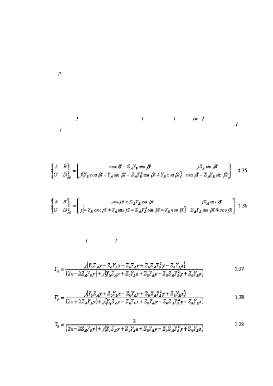
2.4.Behaviour of S-parameters verses frequency

In order to define the behaviour of the s-parameters with the frequency change we follow

the following way. Let us consider ABCD matrixes of even and odd mode expressed in (1.12) and

(1.15), respectively. With those matrixes, in order to calculate s-parameters in center frequency we

have taken

β

value as

π

/2 and therefore cos

β

was 0 and sin

β

was 1 (

β

2

π

/

λ

and

λ

=

ν

p

/

ƒ

). In this

case since we will observe the dependence of s-parameters to the frequency we will take sin

β

and

cos

β

as they are and calculate s-parameters with them.

Solving (1.12) and (1.15), then ABCD matrixes are:

Solving for

Γ

e

,

Γ

o

, T

e

, T

o

:

Putting x for cos

β

and y for sin

β

in the equations;

At this point, if we use (1.25), (1.26), (1.27), (1.28), then we get all the necessary s-parameters in
our hand. After finding s-parameters, we can find magnitude of s-parameters and plot the

magnitude verses frequency plot. This simulation program can plot the magnitude of s-parameters

vs. frequency plot.

References:

1. Fooks, E. H. Microwave engineering using microstrip circuits, Prentice Hall New York 1990

2. Pozar, David M. Microwave Engineering Second Edition, Wiley, New York 1998