
Lattices and Topology
Guram Bezhanishvili and Mamuka Jibladze
ESSLLI’08
11-15.VIII.2008
Lecture 1: Basics of lattice theory

Introduction
Lattice Theory
is a relatively new branch of mathematics, which
lies on the interface of algebra and logic.
The origins of lattice theory can be traced back to
George Boole
(1815 – 1864) (“An Investigation of the Laws of Thought...”,
1854).
Richard Dedekind
(1831 - 1916), in a series of papers around
1900, laid foundation of lattice theory.
But it wasn’t until the 1930ies and 1940ies that lattice theory
became an independent branch of mathematics with its own
internal problematics, thanks to the work of such
mathematicians as
Garett Birkhoff
(1911 – 1996),
Marshall
Stone
(1903 - 1989) ,
Alfred Tarski
(1902 - 1983), and
Robert
Dilworth
(1914 - 1993).
Further advances in lattice theory were obtained by
Bjarni
J´
onsson
,
Bernhard Banaschewski
,
George Gr¨
atzer
, and many
many others..

Introduction
Why is Lattice Theory useful for logic??
Well..
Lattices encode algebraic behavior of the
entailment
relation
and such basic logical connectives as “
and
” (∧,
conjunction) and “
or
” (∨, disjunction).
Relationship between syntax and semantics is likewise
reflected in the relationship between lattices and their
dual
spaces
.
Duals are used to provide various useful
representation
theorems
for lattices, which reflect various
completeness
results
in logic. We will address this issue in detail in
Lecture 5.

Introduction
Why is Lattice Theory useful for logic??
Well..
Lattices encode algebraic behavior of the
entailment
relation
and such basic logical connectives as “
and
” (∧,
conjunction) and “
or
” (∨, disjunction).
Relationship between syntax and semantics is likewise
reflected in the relationship between lattices and their
dual
spaces
.
Duals are used to provide various useful
representation
theorems
for lattices, which reflect various
completeness
results
in logic.
We will address this issue in detail in
Lecture 5.

Introduction
Why is Lattice Theory useful for logic??
Well..
Lattices encode algebraic behavior of the
entailment
relation
and such basic logical connectives as “
and
” (∧,
conjunction) and “
or
” (∨, disjunction).
Relationship between syntax and semantics is likewise
reflected in the relationship between lattices and their
dual
spaces
.
Duals are used to provide various useful
representation
theorems
for lattices, which reflect various
completeness
results
in logic. We will address this issue in detail in
Lecture 5.

Introduction
Our aim is to give a systematic yet elementary account of basics
of lattice theory and its connection to topology.
After providing the necessary prerequisites, we will describe the
dual spaces of distributive lattices, and the representation
theorems provided by the duality.
The logical significance of these theorems lies in the fact that
they are essentially equivalent to results about relational and
topological completeness of some well-known propositional
calculi.
Outline
Lecture 1: Basics of lattice theory
Partial orders and lattices
Lattices as algebras
Distributive laws, Birkhoff’s characterization of distributive
lattices
Boolean lattices and Heyting lattices
Lecture 2: Representation of distributive lattices
Join-prime and meet-prime elements
Birkhoff’s duality between finite distributive lattices and
finite posets
Prime filters and prime ideals
Representation of distributive lattices
Outline
Lecture 3: Topology
Topological spaces
Closure and interior
Separation axioms
Compactness
Compact Hausdorff spaces
Stone spaces
Lecture 4: Duality
Priestley duality for distributive lattices
Stone duality for Boolean lattices
Esakia duality for Heyting lattices
Lecture 5: Spectral duality and applications to logic
Spectral duality
Distributive lattices in logic
Relational completeness of IPC and CPC
Topological completeness of IPC and CPC

Posets
A pair (P, 6) is called a
poset
(shorthand for
p
artially
o
rdered
s
et) if P is a nonempty set and 6 is a
partial order
on P; that is
6 is a binary relation on P which is
reflexive
,
antisymmetric
,
and
transitive
.
Reflexive
: p 6 p for all p ∈ P.
Antisymmetric
: If p 6 q and q 6 p, then p = q for all
p, q ∈ P.
Transitive
: If p 6 q and q 6 r, then p 6 r for all p, q, r ∈ P.

Hasse diagrams
There is a very useful way to depict posets using the so called
Hasse diagrams
.
Rough idea:
To indicate p 6 q, we picture p somewhere below
q, and draw a line connecting p with q. To make pictures easy to
draw and understand, if p 6 q and q 6 r, we only draw lines
connecting p and q, and q and r, and don’t draw a connecting
line between p and r.
Of course, p 6 r by transitivity, but connecting p and r by a line
would make the diagram messy, so we avoid it. By the same
reason, we don’t draw a loop connecting p with itself.

Hasse diagrams
There is a very useful way to depict posets using the so called
Hasse diagrams
.
Rough idea:
To indicate p 6 q, we picture p somewhere below
q, and draw a line connecting p with q.
To make pictures easy to
draw and understand, if p 6 q and q 6 r, we only draw lines
connecting p and q, and q and r, and don’t draw a connecting
line between p and r.
Of course, p 6 r by transitivity, but connecting p and r by a line
would make the diagram messy, so we avoid it. By the same
reason, we don’t draw a loop connecting p with itself.

Hasse diagrams
There is a very useful way to depict posets using the so called
Hasse diagrams
.
Rough idea:
To indicate p 6 q, we picture p somewhere below
q, and draw a line connecting p with q. To make pictures easy to
draw and understand, if p 6 q and q 6 r, we only draw lines
connecting p and q, and q and r, and don’t draw a connecting
line between p and r.
Of course, p 6 r by transitivity, but connecting p and r by a line
would make the diagram messy, so we avoid it. By the same
reason, we don’t draw a loop connecting p with itself.

Hasse diagrams
There is a very useful way to depict posets using the so called
Hasse diagrams
.
Rough idea:
To indicate p 6 q, we picture p somewhere below
q, and draw a line connecting p with q. To make pictures easy to
draw and understand, if p 6 q and q 6 r, we only draw lines
connecting p and q, and q and r, and don’t draw a connecting
line between p and r.
Of course, p 6 r by transitivity, but connecting p and r by a line
would make the diagram messy, so we avoid it.
By the same
reason, we don’t draw a loop connecting p with itself.

Hasse diagrams
There is a very useful way to depict posets using the so called
Hasse diagrams
.
Rough idea:
To indicate p 6 q, we picture p somewhere below
q, and draw a line connecting p with q. To make pictures easy to
draw and understand, if p 6 q and q 6 r, we only draw lines
connecting p and q, and q and r, and don’t draw a connecting
line between p and r.
Of course, p 6 r by transitivity, but connecting p and r by a line
would make the diagram messy, so we avoid it. By the same
reason, we don’t draw a loop connecting p with itself.

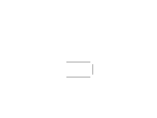
Hasse diagrams
Example
: Let P = {a, b, c, d, e} with
a 6 a
a 6 b
a 6 c
a 6 d
a 6 e
b 6 b
b 6 d
b 6 e
c 6 c
c 6 d
c 6 e
d 6 d
e 6 e.
Then the corresponding Hasse diagram looks like this:
d
e
b
c
???
???
???
???
??
a
????
??

Hasse diagrams
Example
: Let P = {a, b, c, d, e} with
a 6 a
a 6 b
a 6 c
a 6 d
a 6 e
b 6 b
b 6 d
b 6 e
c 6 c
c 6 d
c 6 e
d 6 d
e 6 e.
Then the corresponding Hasse diagram looks like this:
d
e
b
c
???
???
???
???
??
a
????
??

Hasse diagrams
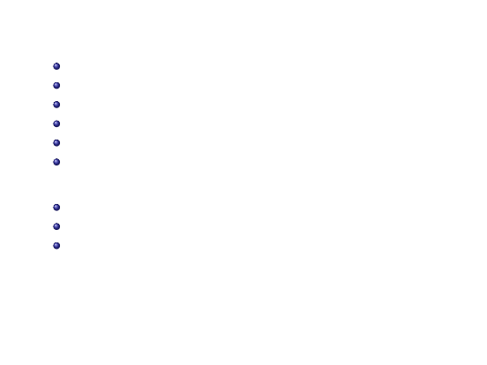
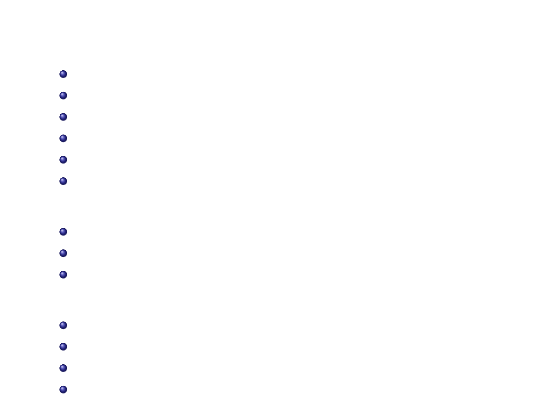
A nonempty set P can be equipped with the simplest (and least
interesting) partial order — the
discrete order
“6”=“=”.
That
is, in (P, =) we have p 6 q if and only if p = q.
The corresponding Hasse diagram does not thus have any lines,
and looks like this:
•
•
•
•
•

Hasse diagrams
A nonempty set P can be equipped with the simplest (and least
interesting) partial order — the
discrete order
“6”=“=”. That
is, in (P, =) we have p 6 q if and only if p = q.
The corresponding Hasse diagram does not thus have any lines,
and looks like this:
•
•
•
•
•

Hasse diagrams
A nonempty set P can be equipped with the simplest (and least
interesting) partial order — the
discrete order
“6”=“=”. That
is, in (P, =) we have p 6 q if and only if p = q.
The corresponding Hasse diagram does not thus have any lines,
and looks like this:
•
•
•
•
•

Hasse diagrams
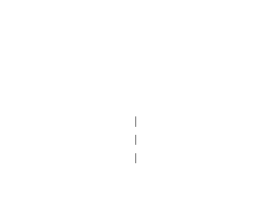
A nonempty set P of real numbers produces a poset by taking
the usual order for “6”. This order is always
linear
.
That is, it
satisfies:
for all p, q ∈ P, either p 6 q or q 6 p.
Hasse diagrams of linear orders look like this:
•
•
•
•

Hasse diagrams
A nonempty set P of real numbers produces a poset by taking
the usual order for “6”. This order is always
linear
. That is, it
satisfies:
for all p, q ∈ P, either p 6 q or q 6 p.
Hasse diagrams of linear orders look like this:
•
•
•
•
Hasse diagrams
A nonempty set P of real numbers produces a poset by taking
the usual order for “6”. This order is always
linear
. That is, it
satisfies:
for all p, q ∈ P, either p 6 q or q 6 p.
Hasse diagrams of linear orders look like this:
•
•
•
•

Order-isomorphisms
Let f : P → Q be a map between two posets P and Q.
We call f
order-preserving
if p 6 q implies f (p) 6 f (q) for each p, q ∈ P.
We call f : P → Q an
order-isomorphism
if f is an
order-preserving 1-1 and onto map such that its inverse is also
order-preserving.
The latter requirement is necessary since there exist 1-1 and
onto order-preserving maps whose inverses aren’t
order-preserving.

Order-isomorphisms
Let f : P → Q be a map between two posets P and Q. We call f
order-preserving
if p 6 q implies f (p) 6 f (q) for each p, q ∈ P.
We call f : P → Q an
order-isomorphism
if f is an
order-preserving 1-1 and onto map such that its inverse is also
order-preserving.
The latter requirement is necessary since there exist 1-1 and
onto order-preserving maps whose inverses aren’t
order-preserving.
Order-isomorphisms
Example
: Consider the following map f : P → Q:
P
Q
•
//
•
•
//
•
It is clearly 1-1 onto order-preserving. However it’s inverse is
not
order-preserving.

Order-isomorphisms
Example
: Consider the following map f : P → Q:
P
Q
•
//
•
•
//
•
It is clearly 1-1 onto order-preserving.
However it’s inverse is
not
order-preserving.

Order-isomorphisms
Example
: Consider the following map f : P → Q:
P
Q
•
//
•
•
//
•
It is clearly 1-1 onto order-preserving. However it’s inverse is
not
order-preserving.

Suprema and infima
Let (P, 6) be a poset. Whenever there exists p ∈ P such that
q 6 p for each q ∈ P, we call p the
largest
or
top
element of P
and denote it by 1.
Similarly, whenever there exists p ∈ P such that p 6 q for each
q ∈ P, we call p the
least
or
bottom
element of P and denote it
by 0.

Suprema and infima
Let (P, 6) be a poset. Whenever there exists p ∈ P such that
q 6 p for each q ∈ P, we call p the
largest
or
top
element of P
and denote it by 1.
Similarly, whenever there exists p ∈ P such that p 6 q for each
q ∈ P, we call p the
least
or
bottom
element of P and denote it
by 0.

Suprema and infima
Let (P, 6) be a poset and let S ⊆ P. We call u ∈ P an
upper
bound
of S if s 6 u for all s ∈ S. We denote the set of upper
bounds of S by S
u
.
Similarly, we call l ∈ P a
lower bound
of S if l 6 s for all s ∈ S.
We denote the set of lower bounds of S by S
l
.
We say that S ⊆ P possesses a
l
east
u
pper
b
ound (shortly
lub
),
or
supremum
, or
join
, if there exists a least element in S
u
.
If S has lub, then we denote it by Sup(S) or
W S.
Similarly, we say that S ⊆ P possesses a
g
reatest
l
ower
b
ound
(shortly
glb
), or
infimum
, or
meet
, if there exists a greatest
element in S
l
.
If S has glb, then we denote it by Inf(S) or
V S.

Lattices
We call a poset (P, 6) a
lattice
if
p ∨ q = Sup{p, q}
and
p ∧ q = Inf{p, q}
exist for all p, q ∈ P.
Examples
:
(1) Here are Hasse diagrams of a couple of finite lattices:
•
•
~
~
~
~
~
~
~
•
•
@@@
@@@
@
•
~
~
~
~
~
~
~
@@@
@@@
@
•
•
•
~
~
~
~
~
~
~
•
@@@
@@@
@
•
~
~
~
~
~
~
~
@@@
@@@
@
Lattices
We call a poset (P, 6) a
lattice
if
p ∨ q = Sup{p, q}
and
p ∧ q = Inf{p, q}
exist for all p, q ∈ P.
Examples
:
(1) Here are Hasse diagrams of a couple of finite lattices:
•
•
~
~
~
~
~
~
~
•
•
@@@
@@@
@
•
~
~
~
~
~
~
~
@@@
@@@
@
•
•
•
~
~
~
~
~
~
~
•
@@@
@@@
@
•
~
~
~
~
~
~
~
@@@
@@@
@

Lattices
(2) Any linearly ordered set is a lattice, where
a ∨ b = max(a, b) =
(
b
if a 6 b,
a
if a > b
and
a ∧ b = min(a, b) =
(
a
if a 6 b,
b
if a > b.
(3) The following posets, however, are
not
lattices:
•
•
~
~
~
~
~
~
~
•
@@@
@@@
@
•
•
•
~
~
~
~
~
~
~
@@@
@@@
@
•
•
•
~
~
~
~
~
~
~
•
@@@
@@@
@

Lattices
(2) Any linearly ordered set is a lattice, where
a ∨ b = max(a, b) =
(
b
if a 6 b,
a
if a > b
and
a ∧ b = min(a, b) =
(
a
if a 6 b,
b
if a > b.
(3) The following posets, however, are
not
lattices:
•
•
~
~
~
~
~
~
~
•
@@@
@@@
@
•
•
•
~
~
~
~
~
~
~
@@@
@@@
@
•
•
•
~
~
~
~
~
~
~
•
@@@
@@@
@

Lattices
Fact: Let L be a lattice. Then all nonempty finite subsets of L
possess suprema and infima.
Proof (Sketch): Let a
1
,
a
2
, ...,
a
n
∈ L. Then an easy induction
gives:
_
{a
1
,
a
2
, ...,
a
n
} = (...(a
1
∨ a
2
) ∨ ...) ∨
a
n
and
^
{a
1
,
a
2
, ...,
a
n
} = (...(a
1
∧ a
2
) ∧ ...) ∧
a
n
.
Therefore,
W {a
1
,
a
2
, ...,
a
n
} and
V {a
1
,
a
2
, ...,
a
n
} exist in L.

Complete lattices
However, there exist lattices L in which not all subsets of L have
suprema and infima.
Examples
:
(1) Let Z be the lattice of all integers with the usual (linear)
ordering. Then the set of positive integers has no supremum
and the set of negative integers has no infimum in Z.
(2) Let N denote the set of non-negative integers. Then the set
P
fin
N of
finite
subsets of N is a lattice with set-theoretic union
and intersection as lattice operations. However, the set of all
finite subsets of
P
fin
N has no supremum.

Complete lattices
However, there exist lattices L in which not all subsets of L have
suprema and infima.
Examples
:
(1) Let Z be the lattice of all integers with the usual (linear)
ordering. Then the set of positive integers has no supremum
and the set of negative integers has no infimum in Z.
(2) Let N denote the set of non-negative integers. Then the set
P
fin
N of
finite
subsets of N is a lattice with set-theoretic union
and intersection as lattice operations.
However, the set of all
finite subsets of
P
fin
N has no supremum.

Complete lattices
However, there exist lattices L in which not all subsets of L have
suprema and infima.
Examples
:
(1) Let Z be the lattice of all integers with the usual (linear)
ordering. Then the set of positive integers has no supremum
and the set of negative integers has no infimum in Z.
(2) Let N denote the set of non-negative integers. Then the set
P
fin
N of
finite
subsets of N is a lattice with set-theoretic union
and intersection as lattice operations. However, the set of all
finite subsets of
P
fin
N has no supremum.

Complete lattices
We call a poset (P, 6) a
complete lattice
if every subset of P has
both supremum and infimum.
Examples:
(1) The interval [0, 1] with the usual (linear) ordering forms a
complete lattice.
(2) The powerset
PX of a set X is a complete lattice with
respect to the order 6=⊆. In fact, for each S ⊆ PX we have
W S = S S and V S = T S.

Complete lattices
We call a lattice
bounded
if it has both top and bottom.
Fact: Every complete lattice is bounded, but not vice versa.
Example:
Let Q be the set of rational numbers, and let
L = [0, 1] ∩ Q. Then L is bounded, but it is
not
complete.

Complete lattices
We call a lattice
bounded
if it has both top and bottom.
Fact: Every complete lattice is bounded, but not vice versa.
Example:
Let Q be the set of rational numbers, and let
L = [0, 1] ∩ Q. Then L is bounded, but it is
not
complete.

Complete lattices
We call a lattice
bounded
if it has both top and bottom.
Fact: Every complete lattice is bounded, but not vice versa.
Example:
Let Q be the set of rational numbers, and let
L = [0, 1] ∩ Q. Then L is bounded, but it is
not
complete.

Lattices as algebras
It turns out that one can equivalently define the lattice structure
on a set purely in terms of the binary operations ∧ and ∨.
Fact: In a lattice, ∨ and ∧ satisfy the following identities:
1
a ∨ b = b ∨ a and a ∧ b = b ∧ a (
commutativity
).
2
(
a ∨ b) ∨ c = a ∨ (b ∨ c) and (a ∧ b) ∧ c = a ∧ (b ∧ c)
(
associativity
).
3
a ∨ a = a = a ∧ a (
idempotency
).
4
a ∧ (a ∨ b) = a = a ∨ (a ∧ b) (
absorption
).
Moreover, a 6 b iff a ∧ b = a iff a ∨ b = b.

Lattices as algebras
Conversely, suppose L is a nonempty set equipped with two
binary operations ∧, ∨ : L × L → L satisfying the identities above.
Then we can define 6 on L as follows:
a 6 b iff a ∧ b = a iff a ∨ b = b.
Fact: We have that 6 is a partial order on L, that
Sup{a, b} = a ∨ b, and that Inf{a, b} = a ∧ b for each a, b ∈ L.
Thus, we can think of lattices as algebras (L, ∨, ∧), where
∨, ∧ : L
2
→ L are two binary operations on L satisfying the
commutativity, associativity, idempotency, and absorption laws.

Lattice homomorphisms and isomorphisms
A map f : L → K between two lattices L and K is called a
lattice
homomorphism
if f (x ∧ y) = f (x) ∧ f (y) and f (x ∨ y) = f (x) ∨ f (y)
for all x, y ∈ L.
That is, f
preserves
∧ and ∨.
Clearly each lattice homomorphism is order-preserving: if x 6 y
then x ∧ y = x; therefore f (x) = f (x ∧ y) = f (x) ∧ f (y), which
means that f (x) 6 f (y).
A
lattice isomorphism
is a 1-1 and onto lattice homomorphism.

Lattice homomorphisms and isomorphisms
A map f : L → K between two lattices L and K is called a
lattice
homomorphism
if f (x ∧ y) = f (x) ∧ f (y) and f (x ∨ y) = f (x) ∨ f (y)
for all x, y ∈ L. That is, f
preserves
∧ and ∨.
Clearly each lattice homomorphism is order-preserving:
if x 6 y
then x ∧ y = x; therefore f (x) = f (x ∧ y) = f (x) ∧ f (y), which
means that f (x) 6 f (y).
A
lattice isomorphism
is a 1-1 and onto lattice homomorphism.

Lattice homomorphisms and isomorphisms
A map f : L → K between two lattices L and K is called a
lattice
homomorphism
if f (x ∧ y) = f (x) ∧ f (y) and f (x ∨ y) = f (x) ∨ f (y)
for all x, y ∈ L. That is, f
preserves
∧ and ∨.
Clearly each lattice homomorphism is order-preserving: if x 6 y
then x ∧ y = x
; therefore f (x) = f (x ∧ y) = f (x) ∧ f (y), which
means that f (x) 6 f (y).
A
lattice isomorphism
is a 1-1 and onto lattice homomorphism.

Lattice homomorphisms and isomorphisms
A map f : L → K between two lattices L and K is called a
lattice
homomorphism
if f (x ∧ y) = f (x) ∧ f (y) and f (x ∨ y) = f (x) ∨ f (y)
for all x, y ∈ L. That is, f
preserves
∧ and ∨.
Clearly each lattice homomorphism is order-preserving: if x 6 y
then x ∧ y = x; therefore f (x) = f (x ∧ y) = f (x) ∧ f (y),
which
means that f (x) 6 f (y).
A
lattice isomorphism
is a 1-1 and onto lattice homomorphism.

Lattice homomorphisms and isomorphisms
A map f : L → K between two lattices L and K is called a
lattice
homomorphism
if f (x ∧ y) = f (x) ∧ f (y) and f (x ∨ y) = f (x) ∨ f (y)
for all x, y ∈ L. That is, f
preserves
∧ and ∨.
Clearly each lattice homomorphism is order-preserving: if x 6 y
then x ∧ y = x; therefore f (x) = f (x ∧ y) = f (x) ∧ f (y), which
means that f (x) 6 f (y).
A
lattice isomorphism
is a 1-1 and onto lattice homomorphism.

Lattice homomorphisms and isomorphisms
A map f : L → K between two lattices L and K is called a
lattice
homomorphism
if f (x ∧ y) = f (x) ∧ f (y) and f (x ∨ y) = f (x) ∨ f (y)
for all x, y ∈ L. That is, f
preserves
∧ and ∨.
Clearly each lattice homomorphism is order-preserving: if x 6 y
then x ∧ y = x; therefore f (x) = f (x ∧ y) = f (x) ∧ f (y), which
means that f (x) 6 f (y).
A
lattice isomorphism
is a 1-1 and onto lattice homomorphism.

Distributive laws
Let L be a lattice and let a, b, c ∈ L. It is easy to see that
(
a ∧ b) ∨ (a ∧ c) 6 a ∧ (b ∨ c)
and that
a ∨ (b ∧ c) 6 (a ∨ b) ∧ (a ∨ c).
We say that in L meet
distributes over join
if for each a, b, c ∈ L
we have
a ∧ (b ∨ c) = (a ∧ b) ∨ (a ∧ c).
Dually, we say that
join distributes over meet
if
a ∨ (b ∧ c) = (a ∨ b) ∧ (a ∨ c).
These laws are called the
distributive laws
.

Distributive laws.
In fact, in every lattice the two distributive laws are equivalent
to each other.
We show that a ∧ (b ∨ c) = (a ∧ b) ∨ (a ∧ c) implies
a ∨ (b ∧ c) = (a ∨ b) ∧ (a ∨ c). The converse is proved similarly.
Suppose a ∧ (b ∨ c) = (a ∧ b) ∨ (a ∧ c) holds in a lattice L. For
p, q, r ∈ L we have:
(
p ∨ q) ∧ (p ∨ r) = [(p ∨ q) ∧ p] ∨ [(p ∨ q) ∧ r]
=
p ∨ ((p ∨ q) ∧ r)
=
p ∨ (r ∧ (p ∨ q))
=
p ∨ [(r ∧ p) ∨ (r ∧ q)]
=
[
p ∨ (r ∧ p)] ∨ (r ∧ q)
=
p ∨ (r ∧ q)
=
p ∨ (q ∧ r).

Distributive lattices
A lattice L is called
distributive
if the above distributive laws
hold in it.
Examples
:
(1) Each linearly ordered set is a distributive lattice.
(2)
P(X) is a distributive lattice for each set X.
(3) Let (P, 6) be a poset. We call A ⊆ P an
upset
of P if x ∈ A
and x 6 y imply y ∈ A. Let U (P) denote the set of upsets of P.
Then (
U (P), ∪, ∩) is a distributive lattice.
Dually, A is called a
downset
of P if x ∈ A and y 6 x imply y ∈ A.
Let
D(P) denote the set of downsets of P. Then (D(P), ∪, ∩) is a
distributive lattice.

Distributive lattices
On the other hand, not every lattice is distributive.
Examples
:
(1) The lattice depicted below, and called the
diamond
, is
not
distributive.
•
•
l
l
l
l
l
l
•
•
RRRRRR
•
l
l
l
l
l
l
RRRRRR
(2) Another non-distributive lattice, called the
pentagon
, is
shown below.
•
•
RRRRRR
•
y
y
y
y
y
y
y
•
•
EEEE
EEE
l
l
l
l
l
l

Birkhoff’s characterization of distributive lattices
The next theorem, due to Birkhoff, says that the diamond and
pentagon are essentially the
only
reason for non-distributivity in
lattices.
Let L be a lattice and S ⊆ L. If for each a, b ∈ S we have
a ∨ b, a ∧ b ∈ S, then we call S a
sublattice
of L. If in addition L is
bounded and 0, 1 ∈ S, then we call S a
bounded sublattice
of L.
We say that a lattice K is
isomorphic to a (bounded) sublattice
S
of L if there exists a (bounded) lattice isomorphism from K onto
S.

Birkhoff’s characterization of distributive lattices
The next theorem, due to Birkhoff, says that the diamond and
pentagon are essentially the
only
reason for non-distributivity in
lattices.
Let L be a lattice and S ⊆ L. If for each a, b ∈ S we have
a ∨ b, a ∧ b ∈ S, then we call S a
sublattice
of L.
If in addition L is
bounded and 0, 1 ∈ S, then we call S a
bounded sublattice
of L.
We say that a lattice K is
isomorphic to a (bounded) sublattice
S
of L if there exists a (bounded) lattice isomorphism from K onto
S.

Birkhoff’s characterization of distributive lattices
The next theorem, due to Birkhoff, says that the diamond and
pentagon are essentially the
only
reason for non-distributivity in
lattices.
Let L be a lattice and S ⊆ L. If for each a, b ∈ S we have
a ∨ b, a ∧ b ∈ S, then we call S a
sublattice
of L. If in addition L is
bounded and 0, 1 ∈ S, then we call S a
bounded sublattice
of L.
We say that a lattice K is
isomorphic to a (bounded) sublattice
S
of L if there exists a (bounded) lattice isomorphism from K onto
S.

Birkhoff’s characterization of distributive lattices
The next theorem, due to Birkhoff, says that the diamond and
pentagon are essentially the
only
reason for non-distributivity in
lattices.
Let L be a lattice and S ⊆ L. If for each a, b ∈ S we have
a ∨ b, a ∧ b ∈ S, then we call S a
sublattice
of L. If in addition L is
bounded and 0, 1 ∈ S, then we call S a
bounded sublattice
of L.
We say that a lattice K is
isomorphic to a (bounded) sublattice
S
of L if there exists a (bounded) lattice isomorphism from K onto
S.

Birkhoff’s characterization of distributive lattices
Birkhoff’ Characterization Theorem: A lattice L is distributive
if and only if neither the diamond nor the pentagon is
isomorphic to a sublattice of L.
Proof (Idea): Clearly if either the diamond or the pentagon can
be embedded into L, then L is non-distributive.
The converse is more difficult to prove.
The rough idea is to
show that if L is not distributive, then we can build either the
diamond or the pentagon inside L. We skip the details.

Boolean lattices
An important subclass of the class of distributive lattices is that
of
Boolean lattices
in which every element has the complement.
Let L be a bounded lattice and a ∈ L. A
complement
of a is an
element b of L such that
a ∨ b = 1 and a ∧ b = 0.
In general a may have several complements or none.

Boolean lattices
An important subclass of the class of distributive lattices is that
of
Boolean lattices
in which every element has the complement.
Let L be a bounded lattice and a ∈ L.
A
complement
of a is an
element b of L such that
a ∨ b = 1 and a ∧ b = 0.
In general a may have several complements or none.

Boolean lattices
An important subclass of the class of distributive lattices is that
of
Boolean lattices
in which every element has the complement.
Let L be a bounded lattice and a ∈ L. A
complement
of a is an
element b of L such that
a ∨ b = 1 and a ∧ b = 0.
In general a may have several complements or none.

Boolean lattices
An important subclass of the class of distributive lattices is that
of
Boolean lattices
in which every element has the complement.
Let L be a bounded lattice and a ∈ L. A
complement
of a is an
element b of L such that
a ∨ b = 1 and a ∧ b = 0.
In general a may have several complements or none.
Boolean lattices
Examples
:
(1) In the diamond, the elements a, b, and c are complements of
each other.
1
a
n
n
n
n
n
n
b
c
OOOOOO
0
o
o
o
o
o
o
PPPPPP
(2) In the pentagon, both x and y are complements of a.
1
y
PPPPPP
a
|
|
|
|
|
|
|
x
0
DDDD
DDD
m
m
m
m
m
m
Boolean lattices
Examples
:
(1) In the diamond, the elements a, b, and c are complements of
each other.
1
a
n
n
n
n
n
n
b
c
OOOOOO
0
o
o
o
o
o
o
PPPPPP
(2) In the pentagon, both x and y are complements of a.
1
y
PPPPPP
a
|
|
|
|
|
|
|
x
0
DDDD
DDD
m
m
m
m
m
m

Boolean lattices
(3) 0 and 1 are always complements of each other.
(4) In a linearly ordered bounded lattice 0 and 1 are the only
elements possessing complements.
Lemma: In a bounded distributive lattice complements are
unique whenever they exist.
Proof: If b and b
0
are both complements of a, then
b = b ∧ 1 = b ∧ (a ∨ b
0
) = (
b ∧ a) ∨ (b ∧ b
0
) =
0 ∨ (b ∧ b
0
) =
b ∧ b
0
Therefore b ≤ b
0
. A similar argument gives us b
0
≤ b. Thus
b = b
0
and so complements are unique whenever they exist.
We denote the complement of a by ¬a.

Boolean lattices
(3) 0 and 1 are always complements of each other.
(4) In a linearly ordered bounded lattice 0 and 1 are the only
elements possessing complements.
Lemma: In a bounded distributive lattice complements are
unique whenever they exist.
Proof: If b and b
0
are both complements of a, then
b = b ∧ 1
=
b ∧ (a ∨ b
0
) = (
b ∧ a) ∨ (b ∧ b
0
) =
0 ∨ (b ∧ b
0
) =
b ∧ b
0
Therefore b ≤ b
0
. A similar argument gives us b
0
≤ b. Thus
b = b
0
and so complements are unique whenever they exist.
We denote the complement of a by ¬a.

Boolean lattices
(3) 0 and 1 are always complements of each other.
(4) In a linearly ordered bounded lattice 0 and 1 are the only
elements possessing complements.
Lemma: In a bounded distributive lattice complements are
unique whenever they exist.
Proof: If b and b
0
are both complements of a, then
b = b ∧ 1 = b ∧ (a ∨ b
0
)
= (
b ∧ a) ∨ (b ∧ b
0
) =
0 ∨ (b ∧ b
0
) =
b ∧ b
0
Therefore b ≤ b
0
. A similar argument gives us b
0
≤ b. Thus
b = b
0
and so complements are unique whenever they exist.
We denote the complement of a by ¬a.

Boolean lattices
(3) 0 and 1 are always complements of each other.
(4) In a linearly ordered bounded lattice 0 and 1 are the only
elements possessing complements.
Lemma: In a bounded distributive lattice complements are
unique whenever they exist.
Proof: If b and b
0
are both complements of a, then
b = b ∧ 1 = b ∧ (a ∨ b
0
) = (
b ∧ a) ∨ (b ∧ b
0
)
=
0 ∨ (b ∧ b
0
) =
b ∧ b
0
Therefore b ≤ b
0
. A similar argument gives us b
0
≤ b. Thus
b = b
0
and so complements are unique whenever they exist.
We denote the complement of a by ¬a.

Boolean lattices
(3) 0 and 1 are always complements of each other.
(4) In a linearly ordered bounded lattice 0 and 1 are the only
elements possessing complements.
Lemma: In a bounded distributive lattice complements are
unique whenever they exist.
Proof: If b and b
0
are both complements of a, then
b = b ∧ 1 = b ∧ (a ∨ b
0
) = (
b ∧ a) ∨ (b ∧ b
0
) =
0 ∨ (b ∧ b
0
)
=
b ∧ b
0
Therefore b ≤ b
0
. A similar argument gives us b
0
≤ b. Thus
b = b
0
and so complements are unique whenever they exist.
We denote the complement of a by ¬a.

Boolean lattices
(3) 0 and 1 are always complements of each other.
(4) In a linearly ordered bounded lattice 0 and 1 are the only
elements possessing complements.
Lemma: In a bounded distributive lattice complements are
unique whenever they exist.
Proof: If b and b
0
are both complements of a, then
b = b ∧ 1 = b ∧ (a ∨ b
0
) = (
b ∧ a) ∨ (b ∧ b
0
) =
0 ∨ (b ∧ b
0
) =
b ∧ b
0
Therefore b ≤ b
0
.
A similar argument gives us b
0
≤ b. Thus
b = b
0
and so complements are unique whenever they exist.
We denote the complement of a by ¬a.

Boolean lattices
(3) 0 and 1 are always complements of each other.
(4) In a linearly ordered bounded lattice 0 and 1 are the only
elements possessing complements.
Lemma: In a bounded distributive lattice complements are
unique whenever they exist.
Proof: If b and b
0
are both complements of a, then
b = b ∧ 1 = b ∧ (a ∨ b
0
) = (
b ∧ a) ∨ (b ∧ b
0
) =
0 ∨ (b ∧ b
0
) =
b ∧ b
0
Therefore b ≤ b
0
. A similar argument gives us b
0
≤ b.
Thus
b = b
0
and so complements are unique whenever they exist.
We denote the complement of a by ¬a.

Boolean lattices
(3) 0 and 1 are always complements of each other.
(4) In a linearly ordered bounded lattice 0 and 1 are the only
elements possessing complements.
Lemma: In a bounded distributive lattice complements are
unique whenever they exist.
Proof: If b and b
0
are both complements of a, then
b = b ∧ 1 = b ∧ (a ∨ b
0
) = (
b ∧ a) ∨ (b ∧ b
0
) =
0 ∨ (b ∧ b
0
) =
b ∧ b
0
Therefore b ≤ b
0
. A similar argument gives us b
0
≤ b. Thus
b = b
0
and so complements are unique whenever they exist.
We denote the complement of a by ¬a.

Boolean lattices
(3) 0 and 1 are always complements of each other.
(4) In a linearly ordered bounded lattice 0 and 1 are the only
elements possessing complements.
Lemma: In a bounded distributive lattice complements are
unique whenever they exist.
Proof: If b and b
0
are both complements of a, then
b = b ∧ 1 = b ∧ (a ∨ b
0
) = (
b ∧ a) ∨ (b ∧ b
0
) =
0 ∨ (b ∧ b
0
) =
b ∧ b
0
Therefore b ≤ b
0
. A similar argument gives us b
0
≤ b. Thus
b = b
0
and so complements are unique whenever they exist.
We denote the complement of a by ¬a.

Boolean lattices
Definition: We call a bounded distributive lattice L a
Boolean
lattice
if each element of L has the complement.
Examples
:
(1) For each set S the lattice
P(S) of all subsets of S is a
Boolean lattice (with usual set-theoretic operations of union,
intersection, and complement).
(2) Let S be an infinite set. We call a subset A of S
cofinite
if
S − A is finite. Let FC(S) denote the set of finite and cofinite
subsets of S. Then it is easy to see that FC(S) is a Boolean lattice
(with usual set-theoretic operations of union, intersection, and
complement).

Boolean lattices
Definition: We call a bounded distributive lattice L a
Boolean
lattice
if each element of L has the complement.
Examples
:
(1) For each set S the lattice
P(S) of all subsets of S is a
Boolean lattice (with usual set-theoretic operations of union,
intersection, and complement).
(2) Let S be an infinite set.
We call a subset A of S
cofinite
if
S − A is finite. Let FC(S) denote the set of finite and cofinite
subsets of S. Then it is easy to see that FC(S) is a Boolean lattice
(with usual set-theoretic operations of union, intersection, and
complement).

Boolean lattices
Definition: We call a bounded distributive lattice L a
Boolean
lattice
if each element of L has the complement.
Examples
:
(1) For each set S the lattice
P(S) of all subsets of S is a
Boolean lattice (with usual set-theoretic operations of union,
intersection, and complement).
(2) Let S be an infinite set. We call a subset A of S
cofinite
if
S − A is finite.
Let FC(S) denote the set of finite and cofinite
subsets of S. Then it is easy to see that FC(S) is a Boolean lattice
(with usual set-theoretic operations of union, intersection, and
complement).

Boolean lattices
Definition: We call a bounded distributive lattice L a
Boolean
lattice
if each element of L has the complement.
Examples
:
(1) For each set S the lattice
P(S) of all subsets of S is a
Boolean lattice (with usual set-theoretic operations of union,
intersection, and complement).
(2) Let S be an infinite set. We call a subset A of S
cofinite
if
S − A is finite. Let FC(S) denote the set of finite and cofinite
subsets of S.
Then it is easy to see that FC(S) is a Boolean lattice
(with usual set-theoretic operations of union, intersection, and
complement).

Boolean lattices
Definition: We call a bounded distributive lattice L a
Boolean
lattice
if each element of L has the complement.
Examples
:
(1) For each set S the lattice
P(S) of all subsets of S is a
Boolean lattice (with usual set-theoretic operations of union,
intersection, and complement).
(2) Let S be an infinite set. We call a subset A of S
cofinite
if
S − A is finite. Let FC(S) denote the set of finite and cofinite
subsets of S. Then it is easy to see that FC(S) is a Boolean lattice
(with usual set-theoretic operations of union, intersection, and
complement).

Heyting lattices
Another important subclass of the class of distributive lattices is
that of
Heyting lattices
.
A
Heyting lattice
is a bounded distributive lattice L such that for
each a, b ∈ L the set
{x ∈ L | a ∧ x 6 b}
has a largest element. As usual, we will denote this element by
a → b and call it the
implication
of a to b.
Thus, in a Heyting lattice L we have:
a ∧ x 6 b iff x 6 a → b
for all a, b, x ∈ L.

Heyting lattices
Another important subclass of the class of distributive lattices is
that of
Heyting lattices
.
A
Heyting lattice
is a bounded distributive lattice L such that for
each a, b ∈ L the set
{x ∈ L | a ∧ x 6 b}
has a largest element.
As usual, we will denote this element by
a → b and call it the
implication
of a to b.
Thus, in a Heyting lattice L we have:
a ∧ x 6 b iff x 6 a → b
for all a, b, x ∈ L.

Heyting lattices
Another important subclass of the class of distributive lattices is
that of
Heyting lattices
.
A
Heyting lattice
is a bounded distributive lattice L such that for
each a, b ∈ L the set
{x ∈ L | a ∧ x 6 b}
has a largest element. As usual, we will denote this element by
a → b
and call it the
implication
of a to b.
Thus, in a Heyting lattice L we have:
a ∧ x 6 b iff x 6 a → b
for all a, b, x ∈ L.

Heyting lattices
Another important subclass of the class of distributive lattices is
that of
Heyting lattices
.
A
Heyting lattice
is a bounded distributive lattice L such that for
each a, b ∈ L the set
{x ∈ L | a ∧ x 6 b}
has a largest element. As usual, we will denote this element by
a → b and call it the
implication
of a to b.
Thus, in a Heyting lattice L we have:
a ∧ x 6 b iff x 6 a → b
for all a, b, x ∈ L.

Heyting lattices
Another important subclass of the class of distributive lattices is
that of
Heyting lattices
.
A
Heyting lattice
is a bounded distributive lattice L such that for
each a, b ∈ L the set
{x ∈ L | a ∧ x 6 b}
has a largest element. As usual, we will denote this element by
a → b and call it the
implication
of a to b.
Thus, in a Heyting lattice L we have:
a ∧ x 6 b iff x 6 a → b
for all a, b, x ∈ L.

Heyting lattices
Examples
:
(1) Each Boolean lattice is a Heyting lattice.
Indeed set
a → b = ¬a ∨ b.
Then a ∧ (¬a ∨ b) = (a ∧ ¬a) ∨ (a ∧ b) = 0 ∨ (a ∧ b) = a ∧ b 6 b.
Moreover if a ∧ x 6 b then
x = 1 ∧ x = (¬a ∨ a) ∧ x = (¬a ∧ x) ∨ (a ∧ x) 6 ¬a ∨ b.

Heyting lattices
Examples
:
(1) Each Boolean lattice is a Heyting lattice. Indeed set
a → b = ¬a ∨ b.
Then a ∧ (¬a ∨ b) = (a ∧ ¬a) ∨ (a ∧ b) = 0 ∨ (a ∧ b) = a ∧ b 6 b.
Moreover if a ∧ x 6 b then
x = 1 ∧ x = (¬a ∨ a) ∧ x = (¬a ∧ x) ∨ (a ∧ x) 6 ¬a ∨ b.

Heyting lattices
Examples
:
(1) Each Boolean lattice is a Heyting lattice. Indeed set
a → b = ¬a ∨ b.
Then a ∧ (¬a ∨ b)
= (
a ∧ ¬a) ∨ (a ∧ b) = 0 ∨ (a ∧ b) = a ∧ b 6 b.
Moreover if a ∧ x 6 b then
x = 1 ∧ x = (¬a ∨ a) ∧ x = (¬a ∧ x) ∨ (a ∧ x) 6 ¬a ∨ b.

Heyting lattices
Examples
:
(1) Each Boolean lattice is a Heyting lattice. Indeed set
a → b = ¬a ∨ b.
Then a ∧ (¬a ∨ b) = (a ∧ ¬a) ∨ (a ∧ b)
=
0 ∨ (a ∧ b) = a ∧ b 6 b.
Moreover if a ∧ x 6 b then
x = 1 ∧ x = (¬a ∨ a) ∧ x = (¬a ∧ x) ∨ (a ∧ x) 6 ¬a ∨ b.

Heyting lattices
Examples
:
(1) Each Boolean lattice is a Heyting lattice. Indeed set
a → b = ¬a ∨ b.
Then a ∧ (¬a ∨ b) = (a ∧ ¬a) ∨ (a ∧ b) = 0 ∨ (a ∧ b)
=
a ∧ b 6 b.
Moreover if a ∧ x 6 b then
x = 1 ∧ x = (¬a ∨ a) ∧ x = (¬a ∧ x) ∨ (a ∧ x) 6 ¬a ∨ b.

Heyting lattices
Examples
:
(1) Each Boolean lattice is a Heyting lattice. Indeed set
a → b = ¬a ∨ b.
Then a ∧ (¬a ∨ b) = (a ∧ ¬a) ∨ (a ∧ b) = 0 ∨ (a ∧ b) = a ∧ b 6 b.
Moreover if a ∧ x 6 b then
x = 1 ∧ x = (¬a ∨ a) ∧ x = (¬a ∧ x) ∨ (a ∧ x) 6 ¬a ∨ b.

Heyting lattices
Examples
:
(1) Each Boolean lattice is a Heyting lattice. Indeed set
a → b = ¬a ∨ b.
Then a ∧ (¬a ∨ b) = (a ∧ ¬a) ∨ (a ∧ b) = 0 ∨ (a ∧ b) = a ∧ b 6 b.
Moreover if a ∧ x 6 b
then
x = 1 ∧ x = (¬a ∨ a) ∧ x = (¬a ∧ x) ∨ (a ∧ x) 6 ¬a ∨ b.

Heyting lattices
Examples
:
(1) Each Boolean lattice is a Heyting lattice. Indeed set
a → b = ¬a ∨ b.
Then a ∧ (¬a ∨ b) = (a ∧ ¬a) ∨ (a ∧ b) = 0 ∨ (a ∧ b) = a ∧ b 6 b.
Moreover if a ∧ x 6 b then
x = 1 ∧ x
= (¬
a ∨ a) ∧ x = (¬a ∧ x) ∨ (a ∧ x) 6 ¬a ∨ b.

Heyting lattices
Examples
:
(1) Each Boolean lattice is a Heyting lattice. Indeed set
a → b = ¬a ∨ b.
Then a ∧ (¬a ∨ b) = (a ∧ ¬a) ∨ (a ∧ b) = 0 ∨ (a ∧ b) = a ∧ b 6 b.
Moreover if a ∧ x 6 b then
x = 1 ∧ x = (¬a ∨ a) ∧ x
= (¬
a ∧ x) ∨ (a ∧ x) 6 ¬a ∨ b.

Heyting lattices
Examples
:
(1) Each Boolean lattice is a Heyting lattice. Indeed set
a → b = ¬a ∨ b.
Then a ∧ (¬a ∨ b) = (a ∧ ¬a) ∨ (a ∧ b) = 0 ∨ (a ∧ b) = a ∧ b 6 b.
Moreover if a ∧ x 6 b then
x = 1 ∧ x = (¬a ∨ a) ∧ x = (¬a ∧ x) ∨ (a ∧ x)
6 ¬a ∨ b.

Heyting lattices
Examples
:
(1) Each Boolean lattice is a Heyting lattice. Indeed set
a → b = ¬a ∨ b.
Then a ∧ (¬a ∨ b) = (a ∧ ¬a) ∨ (a ∧ b) = 0 ∨ (a ∧ b) = a ∧ b 6 b.
Moreover if a ∧ x 6 b then
x = 1 ∧ x = (¬a ∨ a) ∧ x = (¬a ∧ x) ∨ (a ∧ x) 6 ¬a ∨ b.

Heyting lattices
(2) Each finite distributive lattice L is a Heyting lattice.
Indeed
simply set
a → b =
_
{x ∈ L | a ∧ x 6 b}
and use distributivity to show that a ∧ (a → b) 6 b.
This example also shows that the class of Heyting lattices is
properly larger than the class of Boolean lattices.
(3) Each bounded linearly ordered lattice is a Heyting lattice
where
a → b =
(
1
if a 6 b,
b
otherwise.
On the other hand, not every bounded distributive lattice is a
Heyting lattice.

Heyting lattices
(2) Each finite distributive lattice L is a Heyting lattice. Indeed
simply set
a → b =
_
{x ∈ L | a ∧ x 6 b}
and use distributivity to show that a ∧ (a → b) 6 b.
This example also shows that the class of Heyting lattices is
properly larger than the class of Boolean lattices.
(3) Each bounded linearly ordered lattice is a Heyting lattice
where
a → b =
(
1
if a 6 b,
b
otherwise.
On the other hand, not every bounded distributive lattice is a
Heyting lattice.

Heyting lattices
Let L be the lattice shown below:
1
. .
.
a
2
a
1
b
2
????
a
?
?
?
?
b
1
????
0
It is easy to see that L is a complete distributive lattice. However
{x | a ∧ x 6 0}
does not have a largest element. Thus L is not a Heyting lattice.

Heyting lattices
Let L be the lattice shown below:
1
. .
.
a
2
a
1
b
2
????
a
?
?
?
?
b
1
????
0
It is easy to see that L is a complete distributive lattice.
However
{x | a ∧ x 6 0}
does not have a largest element. Thus L is not a Heyting lattice.

Heyting lattices
Let L be the lattice shown below:
1
. .
.
a
2
a
1
b
2
????
a
?
?
?
?
b
1
????
0
It is easy to see that L is a complete distributive lattice. However
{x | a ∧ x 6 0}
does not have a largest element.
Thus L is not a Heyting lattice.

Heyting lattices
Let L be the lattice shown below:
1
. .
.
a
2
a
1
b
2
????
a
?
?
?
?
b
1
????
0
It is easy to see that L is a complete distributive lattice. However
{x | a ∧ x 6 0}
does not have a largest element. Thus L is not a Heyting lattice.

Heyting lattices
Note that the following infinite distributive law fails in L:
(
∧,
W-distributivity
)
a ∧
_
S =
_
{a ∧ s | s ∈ S}
This is exactly the reason that L is not a Heyting lattice because
a complete distributive lattice is a Heyting lattice iff the
(∧,
W)-distributivity holds in it.

Heyting lattices
Note that the following infinite distributive law fails in L:
(
∧,
W-distributivity
)
a ∧
_
S =
_
{a ∧ s | s ∈ S}
This is exactly the reason that L is not a Heyting lattice because
a complete distributive lattice is a Heyting lattice iff the
(∧,
W)-distributivity holds in it.

Heyting lattices
Note that the following infinite distributive law fails in L:
(
∧,
W-distributivity
)
a ∧
_
S =
_
{a ∧ s | s ∈ S}
This is exactly the reason that L is not a Heyting lattice
because
a complete distributive lattice is a Heyting lattice iff the
(∧,
W)-distributivity holds in it.

Heyting lattices
Note that the following infinite distributive law fails in L:
(
∧,
W-distributivity
)
a ∧
_
S =
_
{a ∧ s | s ∈ S}
This is exactly the reason that L is not a Heyting lattice because
a complete distributive lattice is a Heyting lattice iff the
(∧,
W)-distributivity holds in it.
Wyszukiwarka
Podobne podstrony:
Corporate Identity Image and Brands lecture notes
Lattice and Other Graphics in R
Joe Vitale and Brad Yates present Money Beyond Belief Home Tapping System
PEACE, POWER AND PAGODAS in present day cambodia
Routines and Chores Using Present Continous Worksheet
Time Prepositions and Adverbs with Present Perfect
Operator algebras and topology Schick
Human Probiotics and Functioal Foods Presentation
20060605 Questions and Answers at a Presentation 2
Lugo G Differential geometry and physics (lecture notes, web draft, 2006)(61s) MDdg
Gardner Differential geometry and relativity (lecture notes, web draft, 2004) (198s) PGr
Apanasov Geometry and topology of complex hyperbolic and CR manifolds (1997) [sharethefiles com]
Orwell and Huxley lecture
#0170 – Questions and Answers at a Presentation
Thomas, Ward Topology Lecture Notes
więcej podobnych podstron