
Differential Geometry in Physics
Gabriel Lugo
Department of Mathematical Sciences and Statistics
University of North Carolina at Wilmington
c
°1992, 1998, 2006

i
This document was reproduced by the University of North Carolina at Wilmington from a camera
ready copy supplied by the authors. The text was generated on an desktop computer using L
A
TEX.
c
°1992,1998, 2006
All rights reserved. No part of this publication may be reproduced, stored in a retrieval system,
or transmitted, in any form or by any means, electronic, mechanical, photocopying, recording or
otherwise, without the written permission of the author. Printed in the United States of America.

ii

Preface
These notes were developed as a supplement to a course on Differential Geometry at the advanced
undergraduate, first year graduate level, which the author has taught for several years. There are
many excellent texts in Differential Geometry but very few have an early introduction to differential
forms and their applications to Physics. It is the purpose of these notes to bridge some of these
gaps and thus help the student get a more profound understanding of the concepts involved. When
appropriate, the notes also correlate classical equations to the more elegant but less intuitive modern
formulation of the subject.
These notes should be accessible to students who have completed traditional training in Advanced
Calculus, Linear Algebra, and Differential Equations. Students who master the entirety of this
material will have gained enough background to begin a formal study of the General Theory of
Relativity.
Gabriel Lugo, Ph. D.
Mathematical Sciences and Statistics
UNCW
Wilmington, NC 28403
lugo@uncw.edu
iii

iv

Contents
Preface
iii
1 Vectors and Curves
1
1.1 Tangent Vectors . . . . . . . . . . . . . . . . . . . . . . . . . . . . . . . . . . . . . .
1
1.2 Curves in R
3
. . . . . . . . . . . . . . . . . . . . . . . . . . . . . . . . . . . . . . . .
3
1.3 Fundamental Theorem of Curves . . . . . . . . . . . . . . . . . . . . . . . . . . . . .
12
2 Differential Forms
15
2.1 1-Forms . . . . . . . . . . . . . . . . . . . . . . . . . . . . . . . . . . . . . . . . . . .
15
2.2 Tensors and Forms of Higher Rank . . . . . . . . . . . . . . . . . . . . . . . . . . . .
17
2.3 Exterior Derivatives . . . . . . . . . . . . . . . . . . . . . . . . . . . . . . . . . . . .
23
2.4 The Hodge- ∗ Operator . . . . . . . . . . . . . . . . . . . . . . . . . . . . . . . . . . .
25
3 Connections
33
3.1 Frames . . . . . . . . . . . . . . . . . . . . . . . . . . . . . . . . . . . . . . . . . . . .
33
3.2 Curvilinear Coordinates . . . . . . . . . . . . . . . . . . . . . . . . . . . . . . . . . .
35
3.3 Covariant Derivative . . . . . . . . . . . . . . . . . . . . . . . . . . . . . . . . . . . .
38
3.4 Cartan Equations . . . . . . . . . . . . . . . . . . . . . . . . . . . . . . . . . . . . . .
40
4 Theory of Surfaces
43
4.1 Manifolds . . . . . . . . . . . . . . . . . . . . . . . . . . . . . . . . . . . . . . . . . .
43
4.2 The First Fundamental Form . . . . . . . . . . . . . . . . . . . . . . . . . . . . . . .
44
4.3 The Second Fundamental Form . . . . . . . . . . . . . . . . . . . . . . . . . . . . . .
48
4.4 Curvature . . . . . . . . . . . . . . . . . . . . . . . . . . . . . . . . . . . . . . . . . .
51
0

Chapter 1
Vectors and Curves
1.1
Tangent Vectors
1.1 Definition Euclidean n-space R
n
is defined as the set of ordered n-tuples p = (p
1
, . . . , p
n
),
where p
i
∈ R, for each i = 1, . . . , n.
Given any two n-tuples p = (p
1
, . . . , p
n
), q = (q
1
, . . . , q
n
) and any real number c, we define two
operations:
p + q = (p
1
+ q
1
, . . . , p
n
+ q
n
)
(1.1)
cp = (cp
1
, . . . , cp
n
)
With the sum and the scalar multiplication of ordered n-tuples defined this way, Euclidean space
acquires the structure of a vector space of n dimensions
1
.
1.2 Definition Let x
i
be the real valued functions in R
n
such that x
i
(p) = p
i
for any point
p = (p
1
, . . . , p
n
). The functions x
i
are then called the natural coordinates of the the point p. When
the dimension of the space n = 3, we often write: x
1
= x, x
2
= y and x
3
= z.
1.3 Definition A real valued function in R
n
is of class C
r
if all the partial derivatives of the
function up to order r exist and are continuous. The space of infinitely differentiable (smooth)
functions will be denoted by C
∞
(R
n
).
In advanced calculus, vectors are usually regarded as arrows characterized by a direction and a
length. Vectors as thus considered as independent of their location in space. Because of physical
and mathematical reasons, it is advantageous to introduce a notion of vectors that does depend on
location. For example, if the vector is to represent a force acting on a rigid body, then the resulting
equations of motion will obviously depend on the point at which the force is applied.
In a later chapter we will consider vectors on curved spaces. In these cases the positions of the
vectors are crucial. For instance, a unit vector pointing north at the earth’s equator is not at all the
same as a unit vector pointing north at the tropic of Capricorn. This example should help motivate
the following definition.
1.4 Definition A tangent vector X
p
in R
n
, is an ordered pair (X, p). We may regard X as an
ordinary advanced calculus vector and p is the position vector of the foot the arrow.
1
In these notes we will use the following index conventions:
Indices such as i, j, k, l, m, n, run from 1 to n.
Indices such as µ, ν, ρ, σ, run from 0 to n.
Indices such as α, β, γ, δ, run from 1 to 2.
1

2
CHAPTER 1. VECTORS AND CURVES
The collection of all tangent vectors at a point p ∈ R
n
is called the tangent space at p and
will be denoted by T
p
(R
n
). Given two tangent vectors X
p
, Y
p
and a constant c, we can define new
tangent vectors at p by (X + Y )
p
=X
p
+ Y
p
and (cX)
p
= cX
p
. With this definition, it is easy to see
that for each point p, the corresponding tangent space T
p
(R
n
) at that point has the structure of a
vector space. On the other hand, there is no natural way to add two tangent vectors at different
points.
Let U be a open subset of R
n
. The set T (U ) consisting of the union of all tangent vectors at
all points in U is called the tangent bundle. This object is not a vector space, but as we will see
later it has much more structure than just a set.
1.5 Definition A vector field X in U ∈ R
n
is a smooth function from U to T (U ).
We may think of a vector field as a smooth assignment of a tangent vector X
p
to each point in
in U . Given any two vector fields X and Y and any smooth function f , we can define new vector
fields X + Y and f X by
(X + Y )
p
= X
p
+ Y
p
(1.2)
(f X)
p
= f X
p
Remark Since the space of smooth functions is not a field but only a ring, the operations
above give the space of vector fields the structure of a ring module. The subscript notation X
p
to
indicate the location of a tangent vector is sometimes cumbersome. At the risk of introducing some
confusion, we will drop the subscript to denote a tangent vector. Hopefully, it will be clear from the
context whether we are referring to a vector or to a vector field.
Vector fields are essential objects in physical applications. If we consider the flow of a fluid in
a region, the velocity vector field indicates the speed and direction of the flow of the fluid at that
point. Other examples of vector fields in classical physics are the electric, magnetic and gravitational
fields.
1.6 Definition Let X
p
be a tangent vector in an open neighborhood U of a point p ∈ R
n
and
let f be a C
∞
function in U . The directional derivative of f at the point p, in the direction of X
p
,
is defined by
∇
X
(f )(p) = ∇f (p) · X(p),
(1.3)
where ∇f (p) is the gradient of the function f at the point p. The notation
X
p
(f ) = ∇
X
(f )(p)
is also often used in these notes. We may think of a tangent vector at a point as an operator on
the space of smooth functions in a neighborhood of the point. The operator assigns to a function
the directional derivative of the function in the direction of the vector. It is easy to generalize the
notion of directional derivatives to vector fields by defining X(f )(p) = X
p
(f ).
1.7 Proposition If f, g ∈ C
∞
R
n
, a, b ∈ R, and X is a vector field, then
X(af + bg) = aX(f ) + bX(g)
(1.4)
X(f g) = f X(g) + gX(f )
The proof of this proposition follows from fundamental properties of the gradient, and it is found in
any advanced calculus text.
Any quantity in Euclidean space which satisfies relations 1.4 is a called a linear derivation on
the space of smooth functions. The word linear here is used in the usual sense of a linear operator
in linear algebra, and the word derivation means that the operator satisfies Leibnitz’ rule.
1.2. CURVES IN R
3
3
The proof of the following proposition is slightly beyond the scope of this course, but the propo-
sition is important because it characterizes vector fields in a coordinate-independent manner.
1.8 Proposition Any linear derivation on C
∞
(R
n
) is a vector field.
This result allows us to identify vector fields with linear derivations. This step is a big departure
from the usual concept of a “calculus” vector. To a differential geometer, a vector is a linear operator
whose inputs are functions. At each point, the output of the operator is the directional derivative
of the function in the direction of X.
Let p ∈ U be a point and let x
i
be the coordinate functions in U . Suppose that X
p
= (X, p),
where the components of the Euclidean vector X are a
1
, . . . , a
n
. Then, for any function f , the
tangent vector X
p
operates on f according to the formula
X
p
(f ) =
n
X
i=1
a
i
(
∂f
∂x
i
)(p).
(1.5)
It is therefore natural to identify the tangent vector X
p
with the differential operator
X
p
=
n
X
i=1
a
i
(
∂
∂x
i
)(p)
(1.6)
X
p
= a
1
(
∂
∂x
1
)
p
+ . . . + a
n
(
∂
∂x
n
)
p
.
Notation: We will be using Einstein’s convention to suppress the summation symbol whenever
an expression contains a repeated index. Thus, for example, the equation above could be simply
written
X
p
= a
i
(
∂
∂x
i
)
p
.
(1.7)
This equation implies that the action of the vector X
p
on the coordinate functions x
i
yields the com-
ponents a
i
of the vector. In elementary treatments, vectors are often identified with the components
of the vector and this may cause some confusion.
The difference between a tangent vector and a vector field is that in the latter case, the coefficients
a
i
are smooth functions of x
i
. The quantities
(
∂
∂x
1
)
p
, . . . , (
∂
∂x
n
)
p
form a basis for the tangent space T
p
(R
n
) at the point p, and any tangent vector can be written
as a linear combination of these basis vectors. The quantities a
i
are called the contravariant
components of the tangent vector. Thus, for example, the Euclidean vector in R
3
X = 3i + 4j − 3k
located at a point p, would correspond to the tangent vector
X
p
= 3(
∂
∂x
)
p
+ 4(
∂
∂y
)
p
− 3(
∂
∂z
)
p
.
1.2
Curves in R
3
1.9 Definition A curve α(t) in R
3
is a C
∞
map from an open subset of R into R
3
. The curve
assigns to each value of a parameter t ∈ R, a point (x
1
(t), x
2
(t), x
2
(t)) in R
3
U ∈ R
α
7−→ R
3
t 7−→ α(t) = (x
1
(t), x
2
(t), x
2
(t))

4
CHAPTER 1. VECTORS AND CURVES
One may think of the parameter t as representing time, and the curve α as representing the
trajectory of a moving point particle.
1.10 Example Let
α(t) = (a
1
t + b
1
, a
2
t + b
2
, a
3
t + b
3
).
This equation represents a straight line passing through the point p = (b
1
, b
2
, b
3
), in the direction
of the vector v = (a
1
, a
2
, a
3
).
1.11 Example Let
α(t) = (a cos ωt, a sin ωt, bt).
This curve is called a circular helix. Geometrically, we may view the curve as the path described by
the hypotenuse of a triangle with slope b, which is wrapped around a circular cylinder of radius a.
The projection of the helix onto the xy-plane is a circle and the curve rises at a constant rate in the
z-direction.
Occasionally, we will revert to the position vector notation
x(t) = (x
1
(t), x
2
(t), x
3
(t))
(1.8)
which is more prevalent in vector calculus and elementary physics textbooks. Of course, what this
notation really means is
x
i
(t) = (x
i
◦ α)(t),
(1.9)
where x
i
are the coordinate slot functions in an open set in R
3
.
1.12 Definition The derivative α
0
(t) of the curve is called the velocity vector and the second
derivative α
00
(t) is called the acceleration. The length v = kα
0
(t)k of the velocity vector is called
the speed of the curve. The components of the velocity vector are simply given by
V(t) =
dx
dt
=
µ
dx
1
dt
,
dx
2
dt
,
dx
3
dt
,
(1.10)
and the speed is
v =
sµ
dx
1
dt
2
+
µ
dx
2
dt
2
+
µ
dx
3
dt
2
(1.11)
The differential dx of the classical position vector given by
dx =
µ
dx
1
dt
,
dx
2
dt
,
dx
3
dt
dt
(1.12)
is called an infinitesimal tangent vector, and the norm kdxk of the infinitesimal tangent vector
is called the differential of arclength ds. Clearly, we have
ds = kdxk = vdt
(1.13)
As we will see later in this text, the notion of infinitesimal objects needs to be treated in a more
rigorous mathematical setting. At the same time, we must not discard the great intuitive value of
this notion as envisioned by the masters who invented Calculus, even at the risk of some possible
confusion! Thus, whereas in the more strict sense of modern differential geometry, the velocity
vector is really a tangent vector and hence it should be viewed as a linear derivation on the space
of functions, it is helpful to regard dx as a traditional vector which, at the infinitesimal level, gives
a linear approximation to the curve.
1.2. CURVES IN R
3
5
If f is any smooth function on R
3
, we formally define α
0
(t) in local coordinates by the formula
α
0
(t)(f ) |
α(t)
=
d
dt
(f ◦ α) |
t
.
(1.14)
The modern notation is more precise, since it takes into account that the velocity has a vector part
as well as point of application. Given a point on the curve, the velocity of the curve acting on a
function, yields the directional derivative of that function in the direction tangential to the curve at
the point in question.
The diagram below provides a more geometrical interpretation of the the velocity vector for-
mula (1.14). The map α(t) from R to R
3
induces a map α
∗
from the tangent space of R to the
tangent space of R
3
. The image α
∗
(
d
dt
) in T R
3
of the tangent vector
d
dt
is what we call α
0
(t)
α
∗
(
d
dt
) = α
0
(t).
Since α
0
(t) is a tangent vector in R
3
, it acts on functions in R
3
. The action of α
0
(t) on a
function f on R
3
is the same as the action of
d
dt
on the composition f ◦ α. In particular, if we apply
α
0
(t) to the coordinate functions x
i
, we get the components of the the tangent vector, as illustrated
d
dt
∈ T R
α
∗
7−→ T R
3
3 α
0
(t)
↓
↓
R
α
7−→ R
3
x
i
7−→ R
α
0
(t)(x
i
) |
α(t)
=
d
dt
(x
i
◦ α) |
t
.
(1.15)
The map α
∗
on the tangent spaces induced by the curve α is called the push-forward. Many
authors use the notation dα to denote the push-forward, but we prefer to avoid this notation because
most students fresh out of advanced calculus have not yet been introduced to the interpretation of
the differential as a linear map on tangent spaces.
1.13 Definition
If t = t(s) is a smooth, real valued function and α(t) is a curve in R
3
, we say that the curve
β(s) = α(t(s)) is a reparametrization of α.
A common reparametrization of curve is obtained by using the arclength as the parameter. Using
this reparametrization is quite natural, since we know from basic physics that the rate of change of
the arclength is what we call speed
v =
ds
dt
= kα
0
(t)k.
(1.16)
The arc length is obtained by integrating the above formula
s =
Z
kα
0
(t)k dt =
Z
sµ
dx
1
dt
2
+
µ
dx
2
dt
2
+
µ
dx
3
dt
2
dt
(1.17)
In practice it is typically difficult to actually find an explicit arclength parametrization of a
curve since not only does one have calculate the integral, but also one needs to be able to find the
inverse function t in terms of s. On the other hand, from a theoretical point of view, arclength
parametrizations are ideal since any curve so parametrized has unit speed. The proof of this fact is
a simple application of the chain rule and the inverse function theorem.
β
0
(s) = [α(t(s))]
0

6
CHAPTER 1. VECTORS AND CURVES
= α
0
(t(s))t
0
(s)
= α
0
(t(s))
1
s
0
(t(s))
=
α
0
(t(s))
kα
0
(t(s))k
,
and any vector divided by its length is a unit vector. Leibnitz notation makes this even more self
evident
dx
ds
=
dx
dt
dt
ds
=
dx
dt
ds
dt
=
dx
dt
k
dx
dt
k
1.14 Example Let α(t) = (a cos ωt, a sin ωt, bt). Then
V(t) = (−aω sin ωt, aω cos ωt, b),
s(t) =
Z
t
0
p
(−aω sin ωu)
2
+ (aω cos ωu)
2
+ b
2
du
=
Z
t
0
p
a
2
ω
2
+ b
2
du
= ct, where, c =
p
a
2
ω
2
+ b
2
.
The helix of unit speed is then given by
β(s) = (a cos
ωs
c
, a sin
ωs
c
, b
ωs
c
).
Frenet Frames
Let β(s) be a curve parametrized by arc length and let T(s) be the vector
T (s) = β
0
(s).
(1.18)
The vector T (s) is tangential to the curve and it has unit length. Hereafter, we will call T the unit
unit tangent vector. Differentiating the relation
T · T = 1,
(1.19)
we get
2T · T
0
= 0,
(1.20)
so we conclude that the vector T
0
is orthogonal to T . Let N be a unit vector orthogonal to T , and
let κ be the scalar such that
T
0
(s) = κN (s).
(1.21)
We call N the unit normal to the curve, and κ the curvature. Taking the length of both sides of
last equation, and recalling that N has unit length, we deduce that
κ = kT
0
(s)k
(1.22)

1.2. CURVES IN R
3
7
It makes sense to call κ the curvature since, if T is a unit vector, then T
0
(s) is not zero only if the
direction of T is changing. The rate of change of the direction of the tangent vector is precisely what
one would expect to measure how much a curve is curving. In particular, it T
0
= 0 at a particular
point, we expect that at that point, the curve is locally well approximated by a straight line.
We now introduce a third vector
B = T × N,
(1.23)
which we will call the binormal vector. The triplet of vectors (T, N, B) forms an orthonormal set;
that is,
T · T = N · N = B · B = 1
T · N = T · B = N · B = 0.
(1.24)
If we differentiate the relation B · B = 1, we find that B · B
0
= 0, hence B
0
is orthogonal to B.
Furthermore, differentiating the equation T · B = 0, we get
B
0
· T + B · T
0
= 0.
rewriting the last equation
B
0
· T = −T
0
· B = −κN · B = 0,
we also conclude that B
0
must also be orthogonal to T . This can only happen if B
0
is orthogonal to
the T B-plane, so B
0
must be proportional to N . In other words, we must have
B
0
(s) = −τ N (s)
(1.25)
for some quantity τ , which we will call the torsion. The torsion is similar to the curvature in the
sense that it measures the rate of change of the binormal. Since the binormal also has unit length,
the only way one can have a non-zero derivative is if B is changing directions. The quantity B
0
then
measures the rate of change in the up and down direction of an observer moving with the curve
always facing forward in the direction of the tangent vector. The binormal B is something like the
flag in the back of sand dune buggy.
The set of basis vectors {T, N, B} is called the Frenet Frame or the repere mobile (moving
frame). The advantage of this basis over the fixed (i,j,k) basis is that the Frenet frame is naturally
adapted to the curve. It propagates along with the curve with the tangent vector always pointing
in the direction of motion, and the normal and binormal vectors pointing in the directions in which
the curve is tending to curve. In particular, a complete description of how the curve is curving can
be obtained by calculating the rate of change of the frame in terms of the frame itself.
1.15 Theorem Let β(s) be a unit speed curve with curvature κ and torsion τ . Then
T
0
=
κN
N
0
= −κT
τ B
B
0
=
−τ B
.
(1.26)
Proof:
We need only establish the equation for N
0
. Differentiating the equation N · N = 1, we
get 2N · N
0
= 0, so N
0
is orthogonal to N. Hence, N
0
must be a linear combination of T and B.
N
0
= aT + bB.
Taking the dot product of last equation with T and B respectively, we see that
a = N
0
· T, and b = N
0
· B.
8
CHAPTER 1. VECTORS AND CURVES
On the other hand, differentiating the equations N · T = 0, and N · B = 0, we find that
N
0
· T = −N · T
0
= −N · (κN ) = −κ
N
0
· B = −N · B
0
= −N · (−τ N ) = τ.
We conclude that a = −κ, b = τ , and thus
N
0
= −κT + τ B.
The Frenet frame equations (1.26) can also be written in matrix form as shown below.
T
N
B
0
=
0
κ
0
−κ
0
τ
0
−τ
0
T
N
B
.
(1.27)
The group-theoretic significance of this matrix formulation is quite important and we will come
back to this later when we talk about general orthonormal frames. At this time, perhaps it suffices
to point out that the appearance of an antisymmetric matrix in the Frenet equations is not at all
coincidental.
The following theorem provides a computational method to calculate the curvature and torsion
directly from the equation of a given unit speed curve.
1.16 Proposition Let β(s) be a unit speed curve with curvature κ > 0 and torsion τ . Then
κ = kβ
00
(s)k
τ
=
β
0
· [β
00
× β
000
]
β
00
· β
00
(1.28)
Proof: If β(s) is a unit speed curve, we have β
0
(s) = T . Then
T
0
= β
00
(s) = κN,
β
00
· β
00
= (κN ) · (κN ),
β
00
· β
00
= κ
2
κ
2
= kβ
00
k
2
β
000
(s) = κ
0
N + κN
0
= κ
0
N + κ(−κT + τ B)
= κ
0
N + −κ
2
T + κτ B.
β
0
· [β
00
× β
000
] = T · [κN × (κ
0
N + −κ
2
T + κτ B)]
= T · [κ
3
B + κ
2
τ T ]
= κ
2
τ
τ
=
β
0
· [β
00
× β
000
]
κ
2
=
β
0
· [β
00
× β
000
]
β
00
· β
00
1.17 Example Consider a circle of radius r whose equation is given by
α(t) = (r cos t, r sin t, 0).
1.2. CURVES IN R
3
9
Then,
α
0
(t) = (−r sin t, r cos t, 0)
kα
0
(t)k =
p
(−r sin t)
2
+ (r cos t)
2
+ 0
2
=
q
r
2
(sin
2
t + cos
2
t)
= r.
Therefore, ds/dt = r and s = rt, which we recognize as the formula for the length of an arc of circle
of radius t, subtended by a central angle whose measure is t radians. We conclude that
β(s) = (−r sin
s
r
, r cos
s
r
, 0)
is a unit speed reparametrization. The curvature of the circle can now be easily computed
T
= β
0
(s) = (− cos
s
r
, − sin
s
r
, 0)
T
0
= (
1
r
sin
s
r
, −
1
r
cos
s
r
, 0)
κ = kβ
00
k = kT
0
k
=
r
1
r
2
sin
2
s
r
+
1
r
2
cos
2
s
r
+ 0
2
=
r
1
r
2
(sin
2
s
r
+ cos
2
s
r
)
=
1
r
This is a very simple but important example. The fact that for a circle of radius r the curvature
is κ = 1/r could not be more intuitive. A small circle has large curvature and a large circle has small
curvature. As the radius of the circle approaches infinity, the circle locally looks more and more like
a straight line, and the curvature approaches 0. If one were walking along a great circle on a very
large sphere (like the earth) one would be perceive the space to be locally flat.
1.18 Proposition Let α(t) be a curve of velocity V, acceleration A, speed v and curvature κ,
then
V = vT,
A =
dv
dt
T + v
2
κN.
(1.29)
Proof:
Let s(t) be the arclength and let β(s) be a unit speed reparametrization. Then α(t) =
β(s(t)) and by the chain rule
V = α
0
(t)
= β
0
(s(t))s
0
(t)
= vT
A = α
00
(t)
=
dv
dt
T + vT
0
(s(t))s
0
(t)
=
dv
dt
T + v(κN )v
=
dv
dt
T + v
2
κN

10
CHAPTER 1. VECTORS AND CURVES
Equation 1.29 is important in physics. The equation states that a particle moving along a curve
in space feels a component of acceleration along the direction of motion whenever there is a change
of speed, and a centripetal acceleration in the direction of the normal whenever it changes direction.
The centripetal acceleration and any point is
a = v
3
κ =
v
2
r
where r is the radius of a circle which has maximal tangential contact with the curve at the point
in question. This tangential circle is called the osculating circle. The osculating circle can be
envisioned by a limiting process similar to that of the tangent to a curve in differential calculus.
Let p be point on the curve, and let q
1
and q
2
be two nearby points. The three points uniquely
determine a circle. This circle is a “secant” approximation to the tangent circle. As the points q
1
and q
2
approach the point p, the “secant” circle approaches the osculating circle. The osculating
circle always lies in the the T N -plane, which by analogy is called the osculating plane.
1.19 Example (Helix)
β(s) = (a cos
ωs
c
, a sin
ωs
c
,
bs
c
), where c =
p
a
2
ω
2
+ b
2
β
0
(s) = (−
aω
c
sin
ωs
c
,
aω
c
cos
ωs
c
,
b
c
)
β
00
(s) = (−
aω
2
c
2
cos
ω
2
s
c
, −
aω
2
c
2
sin
ωs
c
, 0)
β
000
(s) = (−
aω
3
c
3
cos
ω
2
s
c
, −
aω
3
c
3
sin
ωs
c
, 0)
κ
2
= β
00
· β
00
=
a
2
ω
4
c
4
κ = ±
aω
2
c
2
τ
=
(β
0
β
00
β
000
)
β
00
· β
00
=
b
c
"
−
aω
2
c
2
cos
ωs
c
−
aω
2
c
2
sin
ωs
c
aω
3
c
2
sin
ωs
c
−
aω
3
c
2
cos
ωs
c
#
c
4
a
2
ω
4
.
=
b
c
a
2
ω
5
c
5
c
4
a
2
ω
4
Simplifying the last expression and substituting the value of c, we get
τ
=
bω
a
2
ω
2
+ b
2
κ = ±
aω
2
a
2
ω
2
+ b
2
Notice that if b = 0, the helix collapses to a circle in the xy-plane. In this case, the formulas above
reduce to κ = 1/a and τ = 0. The ratio κ/τ = aω/b is particularly simple. Any curve where
κ/τ = constant is called a helix, of which the circular helix is a special case.
1.20 Example (Plane curves) Let α(t) = (x(t), y(t), 0). Then
α
0
= (x
0
, y
0
, 0)
1.2. CURVES IN R
3
11
α
00
= (x
00
, y
00
, 0)
α
000
= (x
000
, y
000
, 0)
κ =
kα
0
× α
00
k
kα
0
k
3
=
| x
0
y
00
− y
0
x
00
|
(x
02
+ y
02
)
3/2
τ
= 0
1.21 Example (Cornu Spiral) Let β(s) = (x(s), y(s), 0), where
x(s) =
Z
s
0
cos
t
2
2c
2
dt
y(s) =
Z
s
0
sin
t
2
2c
2
dt.
(1.30)
Then, using the fundamental theorem of calculus, we have
β
0
(s) = (cos
s
2
2c
2
, sin
t
2
2c
2
, 0),
Since kβ
0
= v = 1k, the curve is of unit speed, and s is indeed the arc length. The curvature of the
Cornu spiral is given by
κ = | x
0
y
00
− y
0
x
00
|= (β
0
· β
0
)
1/2
= k −
s
c
2
sin
t
2
2c
2
,
s
c
2
cos
t
2
2c
2
, 0k
=
s
c
2
.
The integrals (1.30) defining the coordinates of the Cornu spiral are the classical Frenel Integrals.
These functions, as well as the spiral itself, arise in the computation of the diffraction pattern of a
coherent beam of light by a straight edge.
In cases where the given curve α(t) is not of unit speed, the following proposition provides
formulas to compute the curvature and torsion in terms of α.
1.22 Proposition If α(t) is a regular curve in R
3
, then
κ
2
=
kα
0
× α
00
k
2
kα
0
k
6
(1.31)
τ
=
(α
0
α
00
α
000
)
kα
0
× α
00
k
2
,
(1.32)
where (α
0
α
00
α
000
) is the triple vector product [α ×
0
α
00
] · α
000
.
Proof:
α
0
= vT
α
00
= v
0
T + v
2
κN
α
000
= (v
2
κ)N
0
((s(t))s
0
(t) + . . .
= v
3
κN
0
+ . . .
= v
3
κτ B + . . .
12
CHAPTER 1. VECTORS AND CURVES
The other terms are unimportant here because α
0
× α
00
is proportional to B.
α
0
× α
00
= v
3
κ(T × N ) = v
3
κB
kα
0
× α
00
k = v
3
κ
κ =
kα
0
× α
00
k
v
3
(α
0
× α
00
) · α
000
= v
6
κ
2
τ
τ
=
(α
0
α
00
α
000
)
v
6
κ
2
=
(α
0
α
00
α
000
)
kα
0
× α
00
k
2
1.3
Fundamental Theorem of Curves
Some geometrical insight into the significance of the curvature and torsion can be gained by consid-
ering the Taylor series expansion of an arbitrary unit speed curve β(s) about s = 0.
β(s) = β(0) + β
0
(0)s +
β
00
(0)
2!
s
2
+
β
000
(0)
3!
s
3
+ . . .
(1.33)
Since we are assuming that s is an arclength parameter,
β
0
(0) = T (0) = T
0
β
00
(0) = (κN )(0) = κ
0
N
0
β
000
(0) = (−κ
2
T + κ
0
N + κτ B)(0) = −κ
2
0
T
0
+ κ
0
0
N
0
+ κ
0
τ
0
B
0
Keeping only the lowest terms in the components of T , N , and B, we get the first order Frenet
approximation to the curve
β(s)
.
= β(0) + T
0
s +
1
2
κ
0
N
0
s
2
+
1
6
κ
0
τ
0
B
0
s
3
.
(1.34)
The first two terms represent the linear approximation to the curve. The first three terms
approximate the curve by a parabola which lies in the osculating plane (T N -plane). If κ
0
= 0, then
locally the curve looks like a straight line. If τ
0
= 0, then locally the curve is a plane curve contained
on the osculating plane. In this sense, the curvature measures the deviation of the curve from a
straight line and the torsion (also called the second curvature) measures the deviation of the curve
from a plane curve.
1.23 Theorem (Fundamental Theorem of Curves) Let κ(s) and τ (s), (s > 0) be any two analytic
functions. Then there exists a unique curve (unique up to its position in R
3
) for which s is the
arclength, κ(s) the curvature and τ (s) the torsion.
Proof:
Pick a point in R
3
. By an appropriate translation transformation, we may assume that
this point is the origin. Pick any orthogonal frame {T, N, B}. The curve is then determined uniquely
by its Taylor expansion in the Frenet frame as in equation (1.34).
1.24 Remark It is possible to prove the theorem by just assuming that κ(s) and τ (s) are con-
tinuous. The proof, however, becomes much harder so we prefer the weaker version of the theorem
based on the simplicity of Taylor’s theorem.
1.25 Proposition A curve with κ = 0 is part of a straight line.
We leave the proof as an exercise.

1.3. FUNDAMENTAL THEOREM OF CURVES
13
1.26 Proposition A curve α(t) with τ = 0 is a plane curve.
Proof: If τ = 0, then (α
0
α
00
α
000
) = 0. This means that the three vectors α
0
, α
00
, and α
000
are linearly
dependent and hence there exist functions a
1
(s),a
2
(s) and a
3
(s) such that
a
3
α
000
+ a
2
α
00
+ a
1
α
0
= 0.
This linear homogeneous equation will have a solution of the form
α = c
1
α
1
+ c
2
α
2
+ c
3
,
c
i
= constant vectors.
This curve lies in the plane
(x − c
3
) · n = 0, where n = c
1
× c
2

14
CHAPTER 1. VECTORS AND CURVES
Chapter 2
Differential Forms
2.1
1-Forms
One of the most puzzling ideas in elementary calculus is that of the of the differential. In the usual
definition, the differential of a dependent variable y = f (x) is given in terms of the differential of
the independent variable by dy = f
0
(x)dx. The problem is with the quantity dx. What does ”dx“
mean? What is the difference between ∆x and dx? How much ”smaller“ than ∆x does dx have to
be? There is no trivial resolution to this question. Most introductory calculus texts evade the issue
by treating dx as an arbitrarily small quantity (lacking mathematical rigor) or by simply referring to
dx as an infinitesimal (a term introduced by Newton for an idea that could not otherwise be clearly
defined at the time.)
In this section we introduce linear algebraic tools that will allow us to interpret the differential
in terms of an linear operator.
2.1 Definition Let p ∈ R
n
, and let T
p
(R
n
) be the tangent space at p. A 1-form at p is a linear
map φ from T
p
(R
n
) into R. We recall that such a map must satisfy the following properties:
a)
φ(X
p
) ∈ R,
∀X
p
∈ R
n
(2.1)
b)
φ(aX
p
+ bY
p
) = aφ(X
p
) + bφ(Y
p
),
∀a, b ∈ R, X
p
, Y
p
∈ T
p
(R
n
)
A 1-form is a smooth choice of a linear map φ as above for each point in the space.
2.2 Definition Let f : R
n
→ R be a real-valued C
∞
function. We define the differential df of
the function as the 1-form such that
df (X) = X(f )
(2.2)
for every vector field in X in R
n
.
In other words, at any point p, the differential df of a function is an operator that assigns to a
tangent vector X
p
the directional derivative of the function in the direction of that vector.
df (X)(p) = X
p
(f ) = ∇f (p) · X(p)
(2.3)
In particular, if we apply the differential of the coordinate functions x
i
to the basis vector fields,
we get
dx
i
(
∂
∂x
j
) =
∂x
i
∂x
j
= δ
i
j
(2.4)
The set of all linear functionals on a vector space is called the dual of the vector space. It is
a standard theorem in linear algebra that the dual of a vector space is also a vector space of the
15
16
CHAPTER 2. DIFFERENTIAL FORMS
same dimension. Thus, the space T
?
p
R
n
of all 1-forms at p is a vector space which is the dual of
the tangent space T
p
R
n
. The space T
?
p
(R
n
) is called the cotangent space of R
n
at the point p.
Equation (2.4) indicates that the set of differential forms {(dx
1
)
p
, . . . , (dx
n
)
p
} constitutes the basis
of the cotangent space which is dual to the standard basis {(
∂
∂x
1
)
p
, . . . (
∂
∂x
n
)
p
} of the tangent space.
The union of all the cotangent spaces as p ranges over all points in R
n
is called the cotangent
bundle T
∗
(R
n
).
2.3 Proposition Let f be any smooth function in R
n
and let {x
1
, . . . x
n
} be coordinate functions
in a neighborhood U of a point p. Then, the differential df is given locally by the expression
df
=
n
X
i=1
∂f
∂x
i
dx
i
(2.5)
=
∂f
∂x
i
dx
i
Proof: The differential df is by definition a 1-form, so, at each point, it must be expressible as a
linear combination of the basis elements {(dx
1
)
p
, . . . , (dx
n
)
p
}. Therefore, to prove the proposition,
it suffices to show that the expression 2.5 applied to an arbitrary tangent vector coincides with
definition 2.2. To see this, consider a tangent vector X
p
= a
j
(
∂
∂x
j
)
p
and apply the expression above
as follows:
(
∂f
∂x
i
dx
i
)
p
(X
p
) = (
∂f
∂x
i
dx
i
)(a
j
∂
∂x
j
)(p)
(2.6)
= a
j
(
∂f
∂x
i
dx
i
)(
∂
∂x
j
)(p)
= a
j
(
∂f
∂x
i
∂x
i
∂x
j
)(p)
= a
j
(
∂f
∂x
i
δ
i
j
)(p)
= (
∂f
∂x
i
a
i
)(p)
= ∇f (p) · X(p)
= df (X)(p)
The definition of differentials as linear functionals on the space of vector fields is much more
satisfactory than the notion of infinitesimals, since the new definition is based on the rigorous
machinery of linear algebra. If α is an arbitrary 1-form, then locally
α = a
1
(x)dx
1
+, . . . + a
n
(x)dx
n
,
(2.7)
where the coefficients a
i
are C
∞
functions. A 1-form is also called a covariant tensor of rank
1, or simply a covector. The coefficients (a
1
, . . . , a
n
) are called the covariant components of the
covector. We will adopt the convention to always write the covariant components of a covector with
the indices down. Physicists often refer to the covariant components of a 1-form as a covariant vector
and this causes some confusion about the position of the indices. We emphasize that not all one
forms are obtained by taking the differential of a function. If there exists a function f , such that
α = df , then the one form α is called exact. In vector calculus and elementary physics, exact forms
are important in understanding the path independence of line integrals of conservative vector fields.
As we have already noted, the cotangent space T
∗
p
(R
n
) of 1-forms at a point p has a natural
vector space structure. We can easily extend the operations of addition and scalar multiplication to

2.2. TENSORS AND FORMS OF HIGHER RANK
17
the space of all 1-forms by defining
(α + β)(X) = α(X) + β(X)
(2.8)
(f α)(X) = f α(X)
for all vector fields X and all smooth functions f .
2.2
Tensors and Forms of Higher Rank
As we mentioned at the beginning of this chapter, the notion of the differential dx is not made
precise in elementary treatments of calculus, so consequently, the differential of area dxdy in R
2
, as
well as the differential of surface area in R
3
also need to be revisited in a more rigorous setting. For
this purpose, we introduce a new type of multiplication between forms that not only captures the
essence of differentials of area and volume, but also provides a rich algebraic and geometric structure
generalizing cross products (which make sense only in R
3
) to Euclidean space of any dimension.
2.4 Definition A map φ : T (R
n
) × T (R
n
) −→ R is called a bilinear map on the tangent space,
if it is linear on each slot. That is,
φ(f
1
X
1
+ f
2
X
2
, Y
1
) = f
1
φ(X
1
, Y
1
) + f
2
φ(X
2
, Y
1
)
φ(X
1
, f
1
Y
1
+ f
2
Y
2
) = f
1
φ(X
1
, Y
1
) + f
2
φ(X
1
, Y
2
),
∀X
i
, Y
i
∈ T (R
n
), f
i
∈ C
∞
R
n
.
Tensor Products
2.5 Definition Let α and β be 1-forms. The tensor product of α and β is defined as the bilinear
map α ⊗ β such that
(α ⊗ β)(X, Y ) = α(X)β(Y )
(2.9)
for all vector fields X and Y .
Thus, for example, if α = a
i
dx
i
and β = b
j
dx
j
, then,
(α ⊗ β)(
∂
∂x
k
,
∂
∂x
l
) = α(
∂
∂x
k
)β(
∂
∂x
l
)
= (a
i
dx
i
)(
∂
∂x
k
)(b
j
dx
j
)(
∂
∂x
l
)
= a
i
δ
i
k
b
j
δ
j
l
= a
k
b
l
.
A quantity of the form T = T
ij
dx
i
⊗ dx
j
is called a covariant tensor of rank 2, and we may think
of the set {dx
i
⊗ dx
j
} as a basis for all such tensors. We must caution the reader again that there is
possible confusion about the location of the indices, since physicists often refer to the components
T
ij
as a covariant tensor.
In a similar fashion, one can define the tensor product of vectors X and Y as the bilinear map
X ⊗ Y such that
(X ⊗ Y )(f, g) = X(f )Y (g)
(2.10)
for any pair of arbitrary functions f and g.
If X = a
i ∂
∂x
i
and Y = b
j ∂
∂x
j
, then the components of X ⊗ Y in the basis
∂
∂x
i
⊗
∂
∂x
j
are simply
given by a
i
b
j
. Any bilinear map of the form
T = T
ij
∂
∂x
i
⊗
∂
∂x
j
(2.11)

18
CHAPTER 2. DIFFERENTIAL FORMS
is called a contravariant tensor of rank 2 in R
n
.
The notion of tensor products can easily be generalized to higher rank, and in fact one can have
tensors of mixed ranks. For example, a tensor of contravariant rank 2 and covariant rank 1 in R
n
is
represented in local coordinates by an expression of the form
T = T
ij
k
∂
∂x
i
⊗
∂
∂x
j
⊗ dx
k
.
This object is also called a tensor of type T
2,1
. Thus, we may think of a tensor of type T
2,1
as map
with three input slots. The map expects two functions in the first two slots and a vector in the third
one. The action of the map is bilinear on the two functions and linear on the vector. The output is
a real number. An assignment of a tensor to each point in R
n
is called a tensor field.
Inner Products
Let X = a
i ∂
∂x
i
and Y = b
j ∂
∂x
j
be two vector fields and let
g(X, Y ) = δ
ij
a
i
b
j
.
(2.12)
The quantity g(X, Y ) is an example of a bilinear map that the reader will recognize as the usual dot
product.
2.6 Definition A bilinear map g(X, Y ) on the tangent space is called a vector inner product if
1. g(X, Y ) = g(Y, X),
2. g(X, X) ≥ 0, ∀X,
3. g(X, X) = 0 iff X = 0.
Since we assume g(X, Y ) to be bilinear, an inner product is completely specified by its action on
ordered pairs of basis vectors. The components g
ij
of the inner product are thus given by
g(
∂
∂x
i
,
∂
∂x
j
) = g
ij
,
(2.13)
where g
ij
is a symmetric n × n matrix which we assume to be non-singular. By linearity, it is easy
to see that if X = a
i ∂
∂x
i
and Y = b
j ∂
∂x
j
are two arbitrary vectors, then
g(X, Y ) = g
ij
a
i
b
j
.
In this sense, an inner product can be viewed as a generalization of the dot product. The standard
Euclidean inner product is obtained if we take g
ij
= δ
ij
. In this case, the quantity g(X, X) =k X k
2
gives the square of the length of the vector. For this reason g
ij
is called a metric and g is called a
metric tensor.
Another interpretation of the dot product can be seen if instead one considers a vector X = a
i ∂
∂x
i
and a 1-form α = b
j
dx
j
. The action of the 1-form on the vector gives
α(X) = (b
j
dx
j
)(a
i
∂
∂x
i
)
= b
j
a
i
(dx
j
)(
∂
∂x
i
)
= b
j
a
i
δ
j
i
= a
i
b
i
.

2.2. TENSORS AND FORMS OF HIGHER RANK
19
If we now define
b
i
= g
ij
b
j
,
(2.14)
we see that the equation above can be rewritten as
a
i
b
j
= g
ij
a
i
b
j
,
and we recover the expression for the inner product.
Equation (2.14) shows that the metric can be used as a mechanism to lower indices, thus trans-
forming the contravariant components of a vector to covariant ones. If we let g
ij
be the inverse of
the matrix g
ij
, that is
g
ik
g
kj
= δ
i
j
,
(2.15)
we can also raise covariant indices by the equation
b
i
= g
ij
b
j
.
(2.16)
We have mentioned that the tangent and cotangent spaces of Euclidean space at a particular point
are isomorphic. In view of the above discussion, we see that the metric accepts a dual interpretation;
one as a bilinear pairing of two vectors
g : T (R
n
) × T (R
n
) −→ R
and another as a linear isomorphism
g : T
?
(R
n
) −→ T (R
n
)
that maps vectors to covectors and vice-versa.
In elementary treatments of calculus, authors often ignore the subtleties of differential 1-forms
and tensor products and define the differential of arclength as
ds
2
≡ g
ij
dx
i
dx
j
,
although what is really meant by such an expression is
ds
2
≡ g
ij
dx
i
⊗ dx
j
.
(2.17)
2.7 Example In cylindrical coordinates, the differential of arclength is
ds
2
= dr
2
+ r
2
dθ
2
+ dz
2
.
(2.18)
In this case, the metric tensor has components
g
ij
=
1 0
0
0 r
2
0
0 0
1
.
(2.19)
2.8 Example In spherical coordinates,
x = ρ sin θ cos φ
y = ρ sin θ sin φ
z = ρ cos θ,
(2.20)
and the differential of arclength is given by
ds
2
= dρ
2
+ ρ
2
dθ
2
+ ρ
2
sin
2
θdφ
2
.
(2.21)
In this case the metric tensor has components
g
ij
=
1 0
0
0 ρ
2
0
0 0
ρ
2
sin θ
2
.
(2.22)

20
CHAPTER 2. DIFFERENTIAL FORMS
Minkowski Space
An important object in mathematical physics is the so-called Minkowski space which is defined
as the pair (M
1,3
, gη), where
M
(1,3)
= {(t, x
1
, x
2
, x
3
)| t, x
i
∈ R}
(2.23)
and η is the bilinear map such that
η(X, X) = −t
2
+ (x
1
)
2
+ (x
2
)
2
+ (x
3
)
2
.
(2.24)
The matrix representing Minkowski’s metric η is given by
η = diag(−1, 1, 1, 1),
in which case, the differential of arclength is given by
ds
2
= η
µν
dx
µ
⊗ dx
ν
= −dt ⊗ dt + dx
1
⊗ dx
1
+ dx
2
⊗ dx
2
+ dx
3
⊗ dx
3
= −dt
2
+ (dx
1
)
2
+ (dx
2
)
2
+ (dx
3
)
2
.
(2.25)
Note: Technically speaking, Minkowski’s metric is not really a metric since η(X, X) = 0 does not
imply that X = 0. Non-zero vectors with zero length are called Light-like vectors and they are
associated with with particles that travel at the speed of light (which we have set equal to 1 in our
system of units.)
The Minkowski metric g
µν
and its matrix inverse g
µν
are also used to raise and lower indices in
the space in a manner completely analogous to R
n
. Thus, for example, if A is a covariant vector
with components
A
µ
= (ρ, A
1
, A
2
, A
3
),
then the contravariant components of A are
A
µ
= η
µν
A
ν
= (−ρ, A
1
, A
2
, A
3
)
Wedge Products and n-Forms
2.9 Definition A map φ : T (R
n
) × T (R
n
) −→ R is called alternating if
φ(X, Y ) = −φ(Y, X).
The alternating property is reminiscent of determinants of square matrices that change sign if
any two column vectors are switched. In fact, the determinant function is a perfect example of an
alternating bilinear map on the space M
2×2
of two by two matrices. Of course, for the definition
above to apply, one has to view M
2×2
as the space of column vectors.
2.10 Definition A 2-form φ is a map φ : T (R
n
) × T (R
n
) −→ R which is alternating and
bilinear.
2.11 Definition Let α and β be 1-forms in R
n
and let X and Y be any two vector fields. The
wedge product of the two 1-forms is the map α ∧ β : T (R
n
) × T (R
n
) −→ R, given by the equation
(α ∧ β)(X, Y ) = α(X)β(Y ) − α(Y )β(X).
(2.26)

2.2. TENSORS AND FORMS OF HIGHER RANK
21
2.12 Theorem If α and β are 1-forms, then α ∧ β is a 2-form.
Proof: We break up the proof into the following two lemmas:
2.13 Lemma The wedge product of two 1-forms is alternating.
Proof: Let α and β be 1-forms in R
n
and let X and Y be any two vector fields. Then
(α ∧ β)(X, Y ) = α(X)β(Y ) − α(Y )β(X)
= −(α(Y )β(X) − α(X)β(Y ))
= −(α ∧ β)(Y, X).
2.14 Lemma The wedge product of two 1-forms is bilinear.
Proof:
Consider 1-forms, α, β, vector fields X
1
, X
2
, Y and functions f
1
, F
2
. Then, since the
1-forms are linear functionals, we get
(α ∧ β)(f
1
X
1
+ f
2
X
2
, Y ) = α(f
1
X
1
+ f
2
X
2
)β(Y ) − α(Y )β(f
1
X
1
+ f
2
X
2
)
= [f
1
α(X
1
) + f
2
α(X
2
)]β(Y ) − α(Y )[f
1
β(X
1
) + f
2
α(X
2
)]
= f
1
α(X
1
)β(Y ) + f
2
α(X
2
)β(Y ) + f
1
α(Y )β(X
1
) + f
2
α(Y )β(X
2
)
= f
1
[α(X
1
)β(Y ) + α(Y )β(X
1
)] + f
2
[α(X
2
)β(Y ) + α(Y )β(X
2
)]
= f
1
(α ∧ β)(X
1
, Y ) + f
2
(α ∧ β)(X
2
, Y ).
The proof of linearity on the second slot is quite similar and is left to the reader.
2.15 Corollary If α and β are 1-forms, then
α ∧ β = −β ∧ α.
(2.27)
This last result tells us that wedge products have characteristics similar to cross products of
vectors in the sense that both of these products anti-commute. This means that we need to be
careful to introduce a minus sign every time we interchange the order of the operation. Thus, for
example, we have
dx
i
∧ dx
j
= −dx
j
∧ dx
i
if i 6= j, whereas
dx
i
∧ dx
i
= −dx
i
∧ dx
i
= 0
since any quantity that equals the negative of itself must vanish. The similarity between wedge
products is even more striking in the next proposition but we emphasize again that wedge products
are much more powerful than cross products, because wedge products can be computed in any
dimension.
2.16 Proposition Let α = A
i
dx
i
and β = B
i
dx
i
be any two 1-forms in R
n
. Then
α ∧ β = (A
i
B
j
)dx
i
∧ dx
j
.
(2.28)
Proof: Let X and Y be arbitrary vector fields. Then
(α ∧ β)((X, Y ) = (A
i
dx
i
)(X)(B
j
dx
j
)(Y ) − (A
i
dx
i
)(Y )(B
j
dx
j
)(X)
= (A
i
B
j
)[dx
i
(X)dx
j
(Y ) − dx
i
(Y )dx
j
(X)]
= (A
i
B
j
)(dx
i
∧ dx
j
)(X, Y ).

22
CHAPTER 2. DIFFERENTIAL FORMS
Because of the antisymmetry of the wedge product, the last of the above equations can be written
as
α ∧ β =
n
X
i=1
n
X
j<i
(A
i
B
j
− A
j
B
i
)(dx
i
∧ dx
j
).
In particular, if n = 3, then the coefficients of the wedge product are the components of the cross
product of A = A
1
i + A
2
j + A
3
k and B = B
1
i + B
2
j + B
3
k.
2.17 Example Let α = x
2
dx − y
2
dy and β = dx + dy − 2xydz. Then
α ∧ β
= (x
2
dx − y
2
dy) ∧ (dx + dy − 2xydz)
= x
2
dx ∧ dx + x
2
dx ∧ dy − 2x
3
ydx ∧ dz − y
2
dy ∧ dx − y
2
dy ∧ dy + 2xy
3
dy ∧ dz
= x
2
dx ∧ dy − 2x
3
ydx ∧ dz − y
2
dy ∧ dx + 2xy
3
dy ∧ dz
= (x
2
+ y
2
)dx ∧ dy − 2x
3
ydx ∧ dx + 2xy
3
dy ∧ dz.
2.18 Example Let x = r cos θ and y = r sin θ. Then
dx ∧ dy = (−r sin θdθ + cos θdr) ∧ (r cos θdθ + sin θdr)
= −r sin
2
θdθ ∧ dr + r cos
2
θdr ∧ dθ
= (r cos
2
θ + r sin
2
θ)(dr ∧ dθ)
= r(dr ∧ dθ).
(2.29)
2.19 Remark
1. The result of the last example yields the familiar differential of area in polar coordinates.
2. The differential of area in polar coordinates is a special example of the change of coordinate
theorem for multiple integrals. It is easy to establish that if x = f
1
(u, v) and y = f
2
(u, v), then
dx ∧ dy = det|J|du ∧ dv, where det|J| is the determinant of the Jacobian of the transformation.
3. Quantities such as dxdy and dydz which often appear in calculus, are not well defined. In
most cases, these entities are actually wedge products of 1-forms.
4. We state without proof that all 2-forms φ in R
n
can be expressed as linear combinations of
wedge products of differentials such as
φ = F
ij
dx
i
∧ dx
j
.
(2.30)
In a more elementary (ie, sloppier) treatment of this subject one could simply define 2-forms to
be gadgets which look like the quantity in equation (2.30). With this motivation, we introduce
the next definition.
2.20 Definition A 3-form φ in R
n
is an object of the following type
φ = A
ijk
dx
i
∧ dx
j
∧ dx
k
(2.31)
where we assume that the wedge product of three 1-forms is associative but alternating in the sense
that if one switches any two differentials, then the entire expression changes by a minus sign. We
challenge the reader to come up with a rigorous definition of three forms (or an n-form, for that
matter) in the spirit of multilinear maps. There is nothing really wrong with using definition (2.31).
2.3. EXTERIOR DERIVATIVES
23
This definition however, is coordinate-dependent and differential geometers prefer coordinate-free
definitions, theorems and proofs.
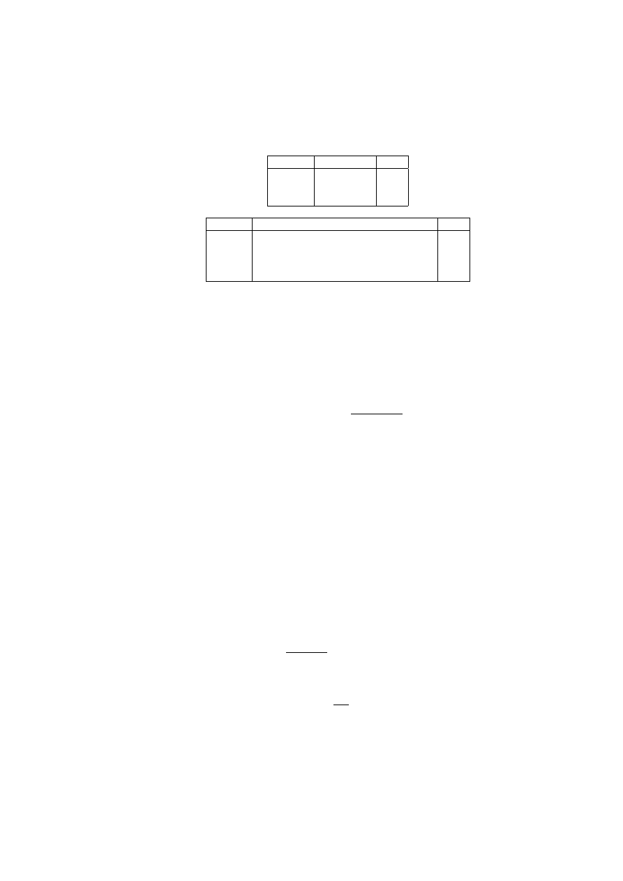
Now for a little combinatorics. Let us count the number of linearly independent differential
forms in Euclidean space. More specifically, we want to find the vector space dimension of the space
of k-forms in R
n
. We will think of 0-forms as being ordinary functions. Since functions are the
”scalars”, the space of 0-forms as a vector space has dimension 1.
R
2
Forms
Dim
0-forms
f
1
1-forms
f dx
1
, gdx
2
2
2-forms
f dx
1
∧ dx
2
1
R
3
Forms
Dim
0-forms
f
1
1-forms
f
1
dx
1
, f
2
dx
2
, f
3
dx
3
3
2-forms
f
1
dx
2
∧ dx
3
, f
2
dx
3
∧ dx
1
, f
3
dx
1
∧ dx
2
3
3-forms
f
1
dx
1
∧ dx
2
∧ dx
3
1
The binomial coefficient pattern should be evident to the reader.
2.3
Exterior Derivatives
In this section we introduce a differential operator that generalizes the classical gradient, curl and
divergence operators.
Denote by
V
m
(p)
(R
n
) the space of m-forms at p ∈ R
n
. This vector space has dimension
dim
V
m
(p)
(R
n
) =
n!
m!(n − m)!
for m ≤ n and dimension 0 for m > n. We will identify
V
0
(p)
(R
n
) with the space of C
∞
functions at
p. The union of all
V
m
(p)
(R
n
) as p ranges through all points in R
n
is called the bundle of m-forms
and will be denoted by
V
m
(R
n
).
A section α of the bundle
V
m
(R
n
) =
[
p
V
m
p
(R
n
).
is called an m-form and it can be written as:
α = A
i
1
,...i
m
(x)dx
i
1
∧ . . . dx
i
m
.
(2.32)
.
2.21 Definition Let α be an m-form (given in coordinates as in equation (2.32)). The exterior
derivative of α is the (m+1-form) dα given by
dα = dA
i
1
,...i
m
∧ dx
i
0
∧ dx
i
1
. . . dx
i
m
=
∂A
i
1
,...i
m
∂dx
i
0
(x)dx
i
0
∧ dx
i
1
. . . dx
i
m
.
(2.33)
In the special case where α is a 0-form, that is, a function, we write
df =
∂f
∂x
i
dx
i
.

24
CHAPTER 2. DIFFERENTIAL FORMS
2.22 Proposition
a)
d :
V
m
−→
V
m+1
b)
d
2
= d ◦ d = 0
c)
d(α ∧ β) = dα ∧ β + (−1)
p
α ∧ dβ
∀α ∈
V
p
, β ∈
V
q
(2.34)
Proof:
a) Obvious from equation (2.33).
b) First, we prove the proposition for α = f ∈
V
0
. We have
d(dα) = d(
∂f
∂dx
i
)
=
∂
2
f
∂x
j
∂x
i
dx
j
∧ dx
i
=
1
2
[
∂
2
f
∂x
j
∂x
i
∂
2
f
∂x
i
∂x
j
]dx
j
∧ dx
i
= 0.
Now, suppose that α is represented locally as in equation (2.32). It follows from equation 2.33
that
d(dα) = d(dA
i
1
,...i
m
) ∧ dx
i
0
∧ dx
i
1
. . . dx
i
m
= 0.
c) Let α ∈
V
p
, β ∈
V
q
. Then, we can write
α = A
i
1
,...i
p
(x)dx
i
1
∧ . . . dx
i
p
β
= B
j
1
,...j
q
(x)dx
j
1
∧ . . . dx
j
q
.
(2.35)
By definition,
α ∧ β = A
i
1
...i
p
B
j
1
...j
q
(dx
i
1
∧ . . . ∧ dx
i
p
) ∧ (dx
j
1
∧ . . . ∧ dx
j
q
).
Now, we take take the exterior derivative of the last equation, taking into account that d(f g) =
f dg + gdf for any functions f and g. We get
d(α ∧ β) = [d(A
i
1
...i
p
)B
j
1
...j
q
+ (A
i
1
...i
p
d(B
j
1
...j
q
)](dx
i
1
∧ . . . ∧ dx
i
p
) ∧ (dx
j
1
∧ . . . ∧ dx
j
q
)
= [dA
i
1
...i
p
∧ (dx
i
1
∧ . . . ∧ dx
i
p
)] ∧ [B
j
1
...j
q
∧ (dx
j
1
∧ . . . ∧ dx
j
q
)] +
= [A
i
1
...i
p
∧ (dx
i
1
∧ . . . ∧ dx
i
p
)] ∧ (−1)
p
[dB
j
1
...j
q
∧ (dx
j
1
∧ . . . ∧ dx
j
q
)]
= dα ∧ β + (−1)
p
α ∧ dβ.
(2.36)
The (−1)
p
factor comes into play since in order to pass the term dB
j
i
...j
p
through p 1-forms of the
type dx
i
, one must perform p transpositions.
2.23 Example Let α = P (x, y)dx + Q(x, y)dβ. Then,
dα = (
∂P
∂x
dx +
∂P
∂y
) ∧ dx + (
∂Q
∂x
dx +
∂Q
∂y
) ∧ dy
=
∂P
∂y
dy ∧ dx +
∂Q
∂x
dx ∧ dy
= (
∂Q
∂x
−
∂P
∂y
)dx ∧ dy.
(2.37)
2.4. THE HODGE- ∗ OPERATOR
25
This example is related to Green’s theorem in R
2
.
2.24 Example Let α = M (x, y)dx + N (x, y)dy, and suppose that dα = 0. Then, by the previous
example,
dα = (
∂N
∂x
−
∂M
∂y
)dx ∧ dy.
Thus, dα = 0 iff N
x
= M
y
, which implies that N = f
y
and M
x
for some function f (x, y). Hence,
α = f
x
dx + f
y
df = df.
The reader should also be familiar with this example in the context of exact differential equations
of first order and conservative force fields.
2.25 Definition A differential form α is called exact if dα = 0.
2.26 Definition A differential form α is called closed if there exists a form β such that α = dβ.
Since d ◦ d = 0, it is clear that an exact form is also closed. For the converse to be true, one must
require a topological condition that the space be contractible. A contractible space is one that can
be deformed continuously to an interior point.
2.27 Poincare’s Lemma In a contractible space (such as R
n
), if a differential is closed, then it
is exact.
The standard counterexample showing that the topological condition in Poincare’s Lemma is
needed is the form dθ where θ is the polar coordinate angle in the plane. It is not hard to prove that
dθ =
−ydx + xdy
x
2
+ y
2
is closed, but not exact in the punctured plane {R
2
\ {0}}.
2.4
The Hodge- ∗ Operator
An important lessons students learn in linear algebra is that all vector spaces of finite dimension n
are isomorphic to each other. Thus, for instance, the space P
3
of all real polynomials in x of degree
3, and the space M
2×2
of real 2 by 2 matrices are, in terms of their vector space properties, basically
no different from the Euclidean vector space R
4
. A good example of this is the tangent space T
p
R
3
which has dimension 3. The process of replacing
∂
∂x
by i,
∂
∂y
by j and
∂
∂z
by k is a linear, 1-1 and
onto map that sends the ”vector“ part of a tangent vector a
1 ∂
∂x
+ a
2 ∂
∂y
+ a
3 ∂
∂z
to regular Eucildean
vector ha
1
, a
2
, a
3
i.
We have also observed that the tangent space T
p
R
n
is isomorphic to the cotangent space T
?
p
R
n
.
In this case, the vector space isomorphism maps the standard basis vectors {
∂
∂x
i
} to their duals
{dx
i
}. This isomorphism then transforms a contravariant vector to a covariant vector. In terms if
components, the isomorphism is provided by the Euclidean metric that maps a the components of
a contravariant vector with indices up to a covariant vector with indices down.
Another interesting example is provided by the spaces
V
1
p
(R
3
) and
V
2
p
(R
3
), both of which have
dimension 3. It follows that these two spaces must be isomorphic. In this case the isomorphism is
given as follows:
dx 7−→ dy ∧ dz
dy 7−→ −dx ∧ dz
dz 7−→ dx ∧ dy
(2.38)
26
CHAPTER 2. DIFFERENTIAL FORMS
More generally, we have seen that the dimension of the space of m-forms in R
n
is given by the
binomial coefficient (
n
m). Since
³ n
m
´
=
µ
n
n − m
=
n!
(n − m)!
,
it must be true that
V
m
p
(R
n
) ∼
=
V
m
p
(R
n−m
).
(2.39)
To describe the isomorphism between these two spaces, we will first need to introduce the totally
antisymmetric Levi-Civita permutation symbol defined as follows:
²
i
1
...i
m
=
+1 if(i
1
, . . . , i
m
) is an even permutation of(1, . . . , m)
−1 if(i
1
, . . . , i
m
) is an odd permutation of(1, . . . , m)
0
otherwise
(2.40)
In dimension 3, there are only 3 (3!=6) nonvanishing components of ²
i,j,k
in
²
123
= ²
231
= ²
312
= 1
²
132
= ²
213
= ²
321
= −1
(2.41)
The permutation symbols are useful in the theory of determinants. In fact, if A = (a
i
j
) is a 3 × 3
matrix, then, using equation (2.41), the reader can easily verify that
detA = |A| = ²
i
1
i
2
i
3
a
i
1
1
a
i
2
2
a
i
3
3
.
(2.42)
This formula for determinants extends in an obvious manner to n × n matrices. A more thorough
discussion of the Levi-Civita symbol will appear later in these notes.
In R
n
, the Levi-Civita symbol with some or all the indices up is numerically equal to the
permutation symbol will all the indices down,
²
i
1
...i
m
= ²
i
1
...i
m
,
since the Euclidean metric used to raise and lower indices is the Kronecker δ
ij
.
On the other hand, in Minkowski space, raising an index with a value of 0 costs a minus sign,
because η
00
= η
00
= −1. Thus, in M
(∞,3)
²
i
0
i
1
i
2
i
3
= −²
i
0
i
1
i
2
i
3
,
since any permutation of {0, 1, 2, 3} must contain a 0.
2.28 Definition The Hodge-∗ operator is a linear map ∗ :
V
m
p
(R
n
) −→
V
m
p
(R
n−m
) defined in
standard local coordinates by the equation,
∗(dx
i
1
∧ . . . ∧ dx
i
m
) =
1
(n − m)!
²
i
1
...i
m
i
m+1
...i
n
dx
i
m+1
∧ . . . ∧ dx
i
m
,
(2.43)
Since the forms dx
i
1
∧. . .∧dx
i
m
constitute a basis of the vector space
V
m
p
(R
n
) and the ∗-operator
is assumed to be a linear map, equation (2.43) completely specifies the map for all m-forms.
2.29 Example Consider the dimension n=3 case. then
∗dx
1
= ²
1
jk
dx
j
∧ dx
k
=
1
2!
[²
1
23
dx
2
∧ dx
3
+ ²
1
32
dx
3
∧ dx
2
]
2.4. THE HODGE- ∗ OPERATOR
27
=
1
2!
[dx
2
∧ dx
3
− dx
3
∧ dx
2
]
=
1
2!
[dx
2
∧ dx
3
+ dx
2
∧ dx
3
]
= dx
2
∧ dx
3
.
We leave it to the reader to complete the computation of the action of the ∗-operator on the other
basis forms. The results are
∗dx
1
= +dx
2
∧ dx
3
∗dx
2
= −dx
1
∧ dx
3
∗dx
3
= +dx
1
∧ dx
2
,
(2.44)
∗(dx
2
∧ dx
3
) = dx
1
∗(−dx
3
∧ dx
1
) = dx
2
∗(dx
1
∧ dx
2
) = dx
3
,
(2.45)
and
∗(dx
1
∧ dx
2
∧ dx
3
) = 1.
(2.46)
In particular, if f : R
3
−→ R is any 0-form (a function), then,
∗f
= f (dx
1
∧ dx
2
∧ dx
3
)
= f dV,
(2.47)
where dV is the differential of volume, also called the volume form.
2.30 Example Let α = A
1
dx
1
A
2
dx
2
+ A
3
dx
3
, and β = B
1
dx
1
B
2
dx
2
+ B
3
dx
3
. Then,
∗(α ∧ β) = (A
2
B
3
− A
3
B
2
) ∗ (dx
2
∧ dx
3
) + (A
1
B
3
− A
3
B
1
) ∗ (dx
1
∧ dx
3
) +
(A
1
B
2
− A
2
B
1
) ∗ (dx
1
∧ dx
2
)
= (A
2
B
3
− A
3
B
2
)dx
1
+ (A
1
B
3
− A
3
B
1
)dx
2
+ (A
1
B
2
− A
2
B
1
)dx
3
= ( ~
A × ~
B)
i
dx
i
(2.48)
The previous examples provide some insight on the action of the ∧ and ∗ operators. If one
thinks of the quantities dx
1
, dx
2
and dx
3
as analogous to ~i, ~j and ~k, then it should be apparent that
equations (2.44) are the differential geometry versions of the well known relations
i = j × k
j = −i × k
k = i × j.
This is even more evident upon inspection of equation (2.48), which relates the ∧ operator to the
Cartesian cross product.
2.31 Example In Minkowski space the collection of all 2-forms has dimension (
4
2
) = 6. The Hodge-
∗ operator in this case splits
V
2
(M
1,3
) into two 3-dim subspaces
V
2
±
, such that ∗ :
V
2
±
−→
V
2
∓
.
More specifically,
V
2
+
is spanned by the forms {dx
0
∧ dx
1
, dx
0
∧ dx
2
, dx
0
∧ dx
3
}, and
V
2
−
is spanned
by the forms {dx
2
∧ dx
3
, −dx
1
∧ dx
3
, dx
1
∧ dx
2
}. The action of ∗ on
V
2
+
is
∗(dx
0
∧ dx
1
) =
1
2
²
01
kl
dx
k
∧ dx
l
= −dx
2
∧ dx
3
∗(dx
0
∧ dx
2
) =
1
2
²
02
kl
dx
k
∧ dx
l
= +dx
1
∧ dx
3
∗(dx
0
∧ dx
3
) =
1
2
²
03
kl
dx
k
∧ dx
l
= −dx
1
∧ dx
2
,
28
CHAPTER 2. DIFFERENTIAL FORMS
and on
V
2
−
,
∗(+dx
2
∧ dx
3
) =
1
2
²
23
kl
dx
k
∧ dx
l
= dx
0
∧ dx
1
∗(−dx
1
∧ dx
3
) =
1
2
²
13
kl
dx
k
∧ dx
l
= dx
0
∧ dx
2
∗(+dx
1
∧ dx
2
) =
1
2
²
12
kl
dx
k
∧ dx
l
= dx
0
∧ dx
3
.
In verifying the equations above, we recall that the Levi-Civita symbols that contain an index with
value 0 in the up position have an extra minus sign as a result of raising the index with η
00
. If
F ∈
V
2
(M), we will formally write F = F
+
+ F
−
, where F
±
∈
V
2
±
. We would like to note that the
action of the dual operator on
V
2
(M) is such that ∗
V
2
(M) −→
V
2
(M), and ∗
2
= −1. In a vector
space a map like ∗ with the property ∗
2
= −1 is a linear involution of the space. In the case in
question
V
2
±
are the eigenspaces corresponding to the +1 and -1 eigenvalues of this involution.
It is also worthwhile to calculate the duals of 1-forms in M
1,3
. The results are
∗dt = −dx
1
∧ dx
2
∧ dx
3
∗dx
1
= +dx
2
∧ dt ∧ dx
3
∗dx
2
= +dt ∧ dx
1
∧ dx
3
∗dx
3
= +dx
1
∧ dt ∧ dx
2
.
(2.49)
Gradient, Curl and Divergence
Classical differential operators that enter in Green’s and Stokes’ Theorems are better understood as
special manifestations of the exterior differential and the Hodge-∗ operators in R
3
. Here is precisely
how this works:
1. Let f : R
3
−→ R be a C
∞
function. Then
df =
∂f
∂x
j
dx
j
= ∇f · dx
(2.50)
2. Let α = A
i
dx
i
be a 1-form in R
3
. Then
(∗d)α =
1
2
(
∂A
i
∂x
j
−
∂A
i
∂x
j
) ∗ (dx
i
∧ dx
j
)
= (∇ × A) · dx
(2.51)
3. Let α = B
1
dx
2
∧ dx
3
+ B
2
dx
3
∧ dx
1
+ B
3
dx
1
∧ dx
2
be a 2-form in R
3
. Then
dα = (
∂B
1
∂x
1
+
∂B
2
∂x
2
+
∂B
3
∂x
3
)dx
1
∧ dx
2
∧ dx
3
= (∇ · B)dV
(2.52)
4. Let α = B
i
dx
i
, then
∗d ∗ α = ∇ · B
(2.53)
It is also possible to define and manipulate formulas of classical vector calculus using the per-
mutation symbols. For example, let a = (A
1
, A
2
, A
3
) and B = (B
1
, B
2
, B
3
) be any two Euclidean
vectors. Then it is easy to see that
(A × B)
k
= ²
ij
k
A
i
B
j
,

2.4. THE HODGE- ∗ OPERATOR
29
and
(∇ × B)
k
= ²
ij
k
∂A
i
∂x
j
,
To derive many classical vector identities in this formalism, it is necessary to first establish the
following identity:
²
ijm
²
klm
= δ
i
k
δ
j
l
− δ
i
l
δ
j
k
.
(2.54)
2.32 Example
[A × (B × C)]
l
= ²
mn
l
A
m
(B × C)
m
= ²
mn
l
A
m
(²
jk
n
B
j
C
k
)
= ²
mn
l
²
jk
n
A
m
B
j
C
k
)
= ²
mnl
²
jkn
A
m
B
j
C
k
)
= (δ
j
l
δ
k
m
− δ
k
l
δ
j
n
)A
m
B
j
C
k
= B
l
A
m
C
m
− C
l
A
m
b
n
,
Or, rewriting in vector form
A × (B × C) = B(A · C) − C(A · B).
(2.55)
Maxwell Equations
The classical equations of Maxwell describing electromagnetic phenomena are
∇ · E = 4πρ ∇ × B = 4πJ +
∂E
∂t
∇ · B = 0
∇ × E = −
∂B
∂t
(2.56)
We would like to formulate these equations in the language of differential forms. Let x
µ
=
(t, x
1
, x
2
, x
3
) be local coordinates in Minkowski’s space M
1,3
. Define the Maxwell 2-form F by the
equation
F =
1
2
F
µν
dx
µ
∧ dx
ν
, (µ, ν = 0, 1, 2, 3),
(2.57)
where
F
µν
=
0 −E
x
−E
y
−E
y
E
x
0
B
z
−B
y
E
y
−B
z
0
B
x
E
z
B
y
−B
x
0
.
(2.58)
Written in complete detail, Maxwell’s 2-form is given by
F
= −E
x
dt ∧ dx
1
− E
y
dt ∧ dx
2
− E
z
dt ∧ dx
3
+
B
z
dx
1
∧ dx
2
− B
y
dx
1
∧ dx
3
+ B
x
dx
2
∧ dx
3
.
(2.59)
We also define the source current 1-form
J = J
µ
dx
µ
= ρdt + J
1
dx
1
+ J
2
dx
2
+ J
3
dx
3
.
(2.60)
2.33 Proposition Maxwell’s Equations (2.56) are equivalent to the equations
dF
= 0,
d ∗ F
= 4π ∗ J.
(2.61)
30
CHAPTER 2. DIFFERENTIAL FORMS
Proof: The proof is by direct computation using the definitions of the exterior derivative and
the Hodge-∗ operator.
dF
= −
∂E
x
∂x
2
∧ dx
2
∧ dt ∧ dx
1
−
∂E
x
∂x
3
∧ dx
3
∧ dt ∧ dx
1
+
−
∂E
y
∂x
1
∧ dx
1
∧ dt ∧ dx
2
−
∂E
y
∂x
3
∧ dx
3
∧ dt ∧ dx
2
+
−
∂E
z
∂x
1
∧ dx
1
∧ dt ∧ dx
3
−
∂E
z
∂x
2
∧ dx
2
∧ dt ∧ dx
3
+
∂B
z
∂t
∧ dt ∧ dx
1
∧ dx
2
−
∂B
z
∂x
3
∧ dx
3
∧ dx
1
∧ dx
2
−
∂B
y
∂t
∧ dt ∧ dx
1
∧ dx
3
−
∂B
y
∂x
2
∧ dx
2
∧ dx
1
∧ dx
3
+
∂B
x
∂t
∧ dt ∧ dx
2
∧ dx
3
+
∂B
x
∂x
1
∧ dx
1
∧ dx
2
∧ dx
3
.
Collecting terms and using the antisymmetry of the wedge operator, we get
dF
= (
∂B
x
∂x
1
+
∂B
y
∂x
2
+
∂B
z
∂x
3
)dx
1
∧ dx
2
∧ dx
3
+
(
∂E
y
∂x
3
−
∂E
z
∂x
2
−
∂B
x
∂t
)dx
2
∧ dt ∧ dx
3
+
(
∂E
z
∂x
1
−
∂E
x
∂dx
3
−
∂B
y
∂t
)dt ∧ dx
1
∧ x
3
+
(
∂E
x
∂x
2
−
∂E
y
∂x
1
−
∂B
z
∂t
)dx
1
∧ dt ∧ dx
2
.
Therefore, dF = 0 iff
∂B
x
∂x
1
+
∂B
y
∂x
2
+
∂B
y
∂x
3
= 0,
which is the same as
∇ · B = 0,
and
∂E
y
∂x
3
−
∂E
z
∂x
2
−
∂B
x
∂x
1
= 0,
∂E
z
∂x
1
−
∂E
x
∂x
3
−
∂B
y
∂x
2
= 0,
∂E
x
∂x
2
−
∂E
y
∂x
1
−
∂B
z
∂x
3
= 0,
which means that
−∇ × E −
∂B
∂t
= 0.
(2.62)
To verify the second set of Maxwell equations, we first compute the dual of the current density
1-form (2.60) using the results from example 2.4. We get
∗J = −ρdx
1
∧ dx
2
∧ dx
3
+ J
1
dx
2
∧ dt ∧ dx
3
+ J
2
dt ∧ dx
1
∧ dx
3
+ J
3
dx
1
∧ dt ∧ dx
2
.
(2.63)
We could now proceed to compute d∗F , but perhaps it is more elegant to notice that F ∈
V
2
(M),
and so, according to example (2.4), F splits into F = F
+
+ F
−
. In fact, we see from (2.58) that the
2.4. THE HODGE- ∗ OPERATOR
31
components of F
+
are those of −E and the components of F
−
constitute the magnetic field vector
B. Using the results of example (2.4), we can immediately write the components of ∗F :
∗F
= B
x
dt ∧ dx
1
+ B
y
dt ∧ dx
2
+ B
z
dt ∧ dx
3
+
E
z
dx
1
∧ dx
2
− E
y
dx
1
∧ dx
3
+ E
x
dx
2
∧ dx
3
,
(2.64)
or equivalently,
F
µν
=
0
B
x
B
y
B
y
−B
x
0
E
z
−E
y
−B
y
−E
z
0
E
x
−B
z
E
y
−E
x
0
.
(2.65)
Since the effect of the dual operator amounts to exchanging
E 7−→ −B
B 7−→ +E,
we can infer from equations (2.62) and (2.63) that
∇ · E = 4πρ
and
∇ × B −
∂E
∂t
= 4πJ.

32
CHAPTER 2. DIFFERENTIAL FORMS
Chapter 3
Connections
Connections
3.1
Frames
As we have already noted in Chapter 1, the theory of curves in R
3
can be elegantly formulated by
introducing orthonormal triplets of vectors which we called Frenet frames. The Frenet vectors are
adapted to the curves in such a manner that the rate of change of the frame gives information about
the curvature of the curve. In this chapter we will study the properties of arbitrary frames and their
corresponding rates of change in the direction of the various vectors in the frame. These concepts
will then be applied later to special frames adapted to surfaces.
3.1 Definition A coordinate frame in R
n
is an n-tuple of vector fields {e
1
, . . . , e
n
} which are
linearly independent at each point p in the space.
In local coordinates x
1
, . . . , x
n
, we can always express the frame vectors as linear combinations
of the standard basis vectors
e
i
= ∂
j
A
j
i
,
(3.1)
where ∂
j
=
∂
∂x
1
. We assume the matrix A = (A
j
i
) to be nonsingular at each point. In linear
algebra, this concept is referred to as a change of basis, the difference being that in our case, the
transformation matrix A depends on the position. A frame field is called orthonormal if at each
point,
< e
i
, e
j
>= δ
ij
.
(3.2)
Throughout this chapter, we will assume that all frame fields are orthonormal. Whereas this
restriction is not necessary, it is convenient because it it results in considerable simplification in
computing the components of an arbitrary vector in the frame.
3.2 Proposition If {e
1
, . . . , e
n
} is an orthonormal frame, then the transformation matrix is
orthogonal (ie, AA
T
= I)
Proof: The proof is by direct computation. Let e
i
= ∂
j
A
j
i
. Then
δ
ij
= < e
i
, e
j
>
= < ∂
k
A
k
i
, ∂
l
A
l
j
>
= A
k
i
A
l
j
< ∂
k
, ∂
l
>
= A
k
i
A
l
j
δ
kl
33
34
CHAPTER 3. CONNECTIONS
= A
k
i
A
kj
= A
k
i
(A
T
)
jk
.
Hence
(A
T
)
jk
A
k
i
= δ
ij
(A
T
)
j
k
A
k
i
= δ
j
i
A
T
A = I
Given a frame vectors e
i
, we can also introduce the corresponding dual coframe forms θ
i
by
requiring that
θ
i
(e
j
) = δ
i
j
.
(3.3)
Since the dual coframe is a set of 1-forms, they can also be expressed in local coordinates as linear
combinations
θ
i
= B
i
k
dx
k
.
It follows from equation( 3.3), that
θ
i
(e
j
) = B
i
k
dx
k
(∂
l
A
l
j
)
= B
i
k
A
l
j
dx
k
(∂
l
)
= B
i
k
A
l
j
δ
k
l
δ
i
j
= B
i
k
A
k
j
.
Therefore, we conclude that BA = I, so B = A
−1
= A
T
. In other words, when the frames are
orthonormal, we have
e
i
= ∂
k
A
k
i
θ
i
= A
i
k
dx
k
.
(3.4)
3.3 Example Consider the transformation from Cartesian to cylindrical coordinates:
x = r cos θ,
y = r sin θ,
z = z.
Using the chain rule for partial derivatives, we have
∂
∂r
= cos θ
∂
∂x
+ sin θ
∂
∂y
∂
∂θ
= −r sin θ
∂
∂x
+ r cos θ
∂
∂y
∂
∂z
=
∂
∂z
From these equations we easily verify that the quantities
e
1
=
∂
∂r
e
2
=
1
r
∂
∂θ
e
3
=
∂
∂z
,
3.2. CURVILINEAR COORDINATES
35
are a triplet of mutually orthogonal unit vectors and thus constitute an orthonormal frame.
3.4 Example For spherical coordinates( 2.20)
x = ρ sin θ cos φ
y = ρ sin θ sin φ
z = ρ cos θ,
the chain rule leads to
∂
∂ρ
= sin θ cos φ
∂
∂x
+ sin θ sin φ
∂
∂y
+ cos θ
∂
∂z
∂
∂θ
= ρ cos θ cos φ
∂
∂x
+ ρ cos θ sin φ
∂
∂y
+ −ρ sin θ
∂
∂z
∂
∂φ
= −ρ sin θ sin φ
∂
∂x
+ ρ sin θ cos φ
∂
∂y
.
In this case, the vectors
e
1
=
∂
∂ρ
e
2
=
1
ρ
∂
∂θ
e
3
=
1
ρ sin θ
∂
∂φ
(3.5)
also constitute an orthonormal frame.
The fact that the chain rule in the two situations above leads to orthonormal frames is not
coincidental. The results are related to the orthogonality of the level surfaces x
i
= constant. Since
the level surfaces are orthogonal whenever they intersect, one expects the gradients of the surfaces
to also be orthogonal. Transformations of this type are called triply orthogonal systems.
3.2
Curvilinear Coordinates
Orthogonal transformations such as spherical and cylindrical coordinates appear ubiquitously in
mathematical physics because the geometry of a large number of problems in this area exhibit sym-
metry with respect to an axis or to the origin. In such situations, transformations to the appropriate
coordinate system often result in considerable simplification of the field equations involved in the
problem. It has been shown that the Laplace operator that appears in the the potential, heat, wave
equation, and Schrdinger field equations is separable in twelve orthogonal coordinate systems. A
simple and efficient method to calculate the Laplacian in orthogonal coordinates can be implemented
using differential forms.
3.5 Example In spherical coordinates the differential of arc length is given by (see equation 2.21)
the metric:
ds
2
= dρ
2
+ ρ
2
dθ
2
+ ρ
2
sin
2
θdφ
2
.
Let
θ
1
= dρ
θ
2
= ρdθ
θ
3
= ρ sin θdφ.
(3.6)
36
CHAPTER 3. CONNECTIONS
Note that these three 1-forms constitute the dual coframe to the orthonormal frame derived in
equation( 3.5). Consider a scalar field f = f (ρ, θ, φ). We now calculate the Laplacian of f in
spherical coordinates using the methods of section 2.4. To do this, we first compute the differential
df and express the result in terms of the coframe.
df
=
∂f
∂ρ
dρ +
∂f
∂θ
dθ +
∂f
∂φ
dφ
=
∂f
∂ρ
θ
1
+
1
ρ
∂f
∂θ
θ
2
+
1
ρ sin θ
∂f
∂φ
θ
3
The components df in the coframe represent the gradient in spherical coordinates. Continuing with
the scheme of section 2.4, we next apply the Hodge-∗ operator. Then, we rewrite the resulting
2-form in terms of wedge products of coordinate differentials so that we can apply the definition of
the exterior derivative.
∗df
=
∂f
∂ρ
θ
2
∧ θ
3
−
1
ρ
∂f
∂θ
θ
1
∧ θ
3
+
1
ρ sin θ
∂f
∂φ
θ
1
∧ θ
2
= ρ
2
sin θ
∂f
∂ρ
dθ ∧ dφ − ρ sin θ
1
ρ
∂f
∂θ
dρ ∧ dφ + ρ sin θ
1
ρ sin θ
∂f
∂φ
dρ ∧ dθ
= ρ
2
sin θ
∂f
∂ρ
dθ ∧ dφ − sin θ
∂f
∂θ
dρ ∧ dφ +
∂f
∂φ
dρ ∧ dθ
d ∗ df
=
∂
∂ρ
(ρ
2
sin θ
∂f
∂ρ
)dρ ∧ dθ ∧ dφ −
∂
∂θ
(sin θ
∂f
∂θ
)dθ ∧ dρ ∧ dφ +
∂
∂φ
(
∂f
∂φ
)dφ ∧ dρ ∧ dθ
=
·
sin θ
∂
∂ρ
(ρ
2
∂f
∂ρ
) +
∂
∂θ
(sin θ
∂f
∂θ
) +
∂
2
f
∂φ
2
¸
dρ ∧ dθ ∧ dφ.
Finally, rewriting the differentials back in terms of the the coframe, we get
d ∗ df =
1
ρ
2
sin θ
·
sin θ
∂
∂ρ
(ρ
2
∂f
∂ρ
) +
∂
∂θ
(sin θ
∂f
∂θ
) +
∂
2
f
∂φ
2
¸
θ
1
∧ θ
2
∧ θ
3
.
So, the Laplacian of f is given by
∇
2
f =
1
ρ
2
∂
∂ρ
·
ρ
2
∂f
∂ρ
¸
+
1
ρ
2
sin θ
·
∂
∂θ
(sin θ
∂f
∂θ
) +
∂
2
f
∂φ
2
¸
(3.7)
The derivation of the expression for the spherical Laplacian through the use of differential forms
is elegant and leads naturally to the operator in Sturm Liouville form.
The process above can be carried out for general orthogonal transformations. A change of
coordinates x
i
= x
i
(u
k
) leads to an orthogonal transformation if in the new coordinate system u
k
,
the line metric
ds
2
= g
11
(du
1
)
2
+ g
22
(du
2
)
2
+ g
33
(du
3
)
2
(3.8)
only has diagonal entries. In this case, we choose the coframe
θ
1
=
√
g
11
du
1
= h
1
du
1
θ
2
=
√
g
22
du
2
= h
2
du
2
θ
3
=
√
g
33
du
3
= h
3
du
3
The quantities {h
1
, h
2
, h
3
} are classically called the weights. Please note that, in the interest of
connecting to classical terminology, we have exchanged two indices for one and this will cause small
discrepancies with the index summation convention. We will revert to using a summation symbol
3.2. CURVILINEAR COORDINATES
37
when these discrepancies occur. To satisfy the duality condition θ
i
(e
j
) = δ
i
j
, we must choose the
corresponding frame vectors e
i
as follows:
e
1
=
1
√
g
11
∂
∂u
1
=
1
h
1
∂
∂u
1
e
2
=
1
√
g
22
∂
∂u
2
=
1
h
2
∂
∂u
2
e
3
=
1
√
g
33
∂
∂u
3
=
1
h
3
∂
∂u
3
Gradient. Let f = f (x
i
) and x
i
= x
i
(u
k
). Then
df
=
∂f
∂x
k
dx
k
=
∂f
∂u
i
∂u
i
∂x
k
dx
k
=
∂f
∂u
i
du
i
=
X
i
1
h
i
∂f
∂u
i
θ
i
= e
i
(f )θ
i
.
As expected, the components of the gradient in the coframe θ
i
are the just the frame vectors.
∇ =
µ
1
h
1
∂
∂u
1
,
1
h
2
∂
∂u
2
,
1
h
3
∂
∂u
3
(3.9)
Curl. Let F = (F
1
, F
2
, F
3
) be a classical vector field. Construct the corresponding 1-form F = F
i
θ
i
in the coframe. We calculate the curl using the dual of the exterior derivative.
F
= F
1
θ
1
+ F
2
θ
2
+ F
3
θ
3
= (h
1
F
1
)du
1
+ (h
2
F
2
)du
2
+ (h
3
F
3
)du
3
= (hF )
i
du
i
, where (hF )
i
= h
i
F
i
dF
=
1
2
·
∂(hF )
i
∂u
j
−
∂(hF )
j
∂u
i
¸
du
i
∧ du
j
=
1
h
i
h
j
·
∂(hF )
i
∂u
j
−
∂(hF )
j
∂u
i
¸
dθ
i
∧ dθ
j
∗dF
= ²
ij
k
·
1
h
i
h
j
[
∂(hF )
i
∂u
j
−
∂(hF )
j
∂u
i
]
¸
θ
k
= (∇ × F )
k
θ
k
.
Thus, the components of the curl are
µ
1
h
2
h
3
[
∂(h
3
F
3
)
∂u
2
−
∂(h
2
F
2
)
∂u
3
],
1
h
1
h
3
[
∂(h
3
F
3
)
∂u
1
−
∂(h
1
F
1
)
∂u
3
],
1
h
1
h
2
[
∂(h
1
F
1
)
∂u
2
−
∂(h
2
F
2
)
∂u
1
].
(3.10)
Divergence. As before, let F = F
i
θ
i
and recall that ∇ · F = ∗d ∗ F . The computation yields
F
= F
1
θ
1
+ F
2
θ
2
+ F
3
θ
3
∗F
= F
1
θ
2
∧ θ
3
+ F
2
θ
3
∧ θ
1
+ F
3
θ
1
∧ θ
2
= (h
2
h
3
F
1
)du
2
∧ du
3
+ (h
1
h
3
F
2
)du
3
∧ du
1
+ (h
1
h
2
F
3
)du
1
∧ du
2
d ∗ dF
=
·
∂(h
2
h
3
F
1
)
∂u
1
+
∂(h
1
h
3
F
2
)
∂u
2
+
∂(h
1
h
2
F
3
)
∂u
3
¸
du
1
∧ du
2
∧ du
3
.

38
CHAPTER 3. CONNECTIONS
Therefore,
∇ · F = ∗d ∗ F =
1
h
1
h
2
h
3
·
∂(h
2
h
3
F
1
)
∂u
1
+
∂(h
1
h
3
F
2
)
∂u
2
+
∂(h
1
h
2
F
3
)
∂u
3
¸
.
(3.11)
3.3
Covariant Derivative
In this section we introduce a generalization of directional derivatives. The directional derivative
measures the rate of change of a function in the direction of a vector. What we want is a quantity
which measures the rate of change of a vector field in the direction of another.
3.6 Definition Let X be an arbitrary vector field in R
n
. A map ∇
X
: T (R
n
) −→ T (R
n
) is
called a Koszul connection if it satisfies the following properties:
1. ∇
f X
(Y ) = f ∇
X
Y,
2. ∇
(X
1
+X
2
)
Y = ∇
X
1
Y + ∇
X
2
Y,
3. ∇
X
(Y
1
+ Y
2
) = ∇
X
Y
1
+ ∇
X
Y
2
,
4. ∇
X
f Y = X(f )Y + f ∇
X
Y,
for all vector fields X, X
1
, X
2
, Y, Y
1
, Y
2
∈ T (R
n
) and all smooth functions f . The definition states
that the map ∇
X
is linear on X but behaves like a linear derivation on Y. For this reason, the
quantity ∇
X
Y is called the covariant derivative of Y in the direction of X.
3.7 Proposition Let Y = f
i ∂
∂x
i
be a vector field in R
n
, and let X another C
∞
vector field.
Then the operator given by
∇
X
Y = X(f
i
)
∂
∂x
i
(3.12)
defines a Koszul connection. The proof just requires verification that the four properties above are
satisfied, and it is left as an exercise. The operator defined in this proposition is called the standard
connection compatible with the standard Euclidean metric. The action of this connection on a
vector field Y yields a new vector field whose components are the directional derivatives of the
components of Y .
3.8 Example Let
X = x
∂
∂x
+ xz
∂
∂y
, Y = x
2
∂
∂x
+ xy
2
∂
∂y
.
Then,
∇
X
Y
= X(x
2
)
∂
∂x
+ X(xy
2
)
∂
∂y
= [x
∂
∂x
(x
2
) + xz
∂
∂y
(x
2
)]
∂
∂x
+ [x
∂
∂x
(xy
2
) + xz
∂
∂y
(xy
2
)]
∂
∂y
= 2x
2
∂
∂x
+ (xy
2
+ 2x
2
yz)
∂
∂y
.
3.9 Definition A Koszul connection ∇
X
is compatible with the metric g(Y, Z) =< Y, Z > if
∇
X
< Y, Z >=< ∇
X
Y, Z > + < Y, ∇
X
Z > .
(3.13)
3.3. COVARIANT DERIVATIVE
39
In Euclidean space, the components of the standard frame vectors are constant, and thus their
rates of change in any direction vanish. Let e
i
be arbitrary frame field with dual forms θ
i
. The
covariant derivatives of the frame vectors in the directions of a vector X will in general yield new
vectors. The new vectors must be linear combinations of the the basis vectors as follows:
∇
X
e
1
= ω
1
1
(X)e
1
+ ω
2
1
(X)e
2
+ ω
3
1
(X)e
3
∇
X
e
2
= ω
1
2
(X)e
1
+ ω
2
2
(X)e
2
+ ω
3
2
(X)e
3
∇
X
e
3
= ω
1
3
(X)e
1
+ ω
2
3
(X)e
2
+ ω
3
3
(X)e
3
(3.14)
The coefficients can be more succinctly expressed using the compact index notation,
∇
X
e
i
= e
j
ω
j
i
(X).
(3.15)
It follows immediately that
ω
j
i
(X) = θ
j
(∇
X
e
i
).
(3.16)
Equivalently, one can take the inner product of both sides of equation (3.15) with e
k
to get
< ∇
X
e
i
, e
k
> = < e
j
ω
j
i
(X), e
k
>
= ω
j
i
(X) < e
j
, e
k
>
= ω
j
i
(X)g
jk
Hence,
< ∇
X
e
i
, e
k
>= ω
ki
(X)
(3.17)
The left hand side of the last equation is the inner product of two vectors, so the expression
represents an array of functions. Consequently, the right hand side also represents an array of
functions. In addition, both expressions are linear on X, since by definition ∇
X
is linear on X. We
conclude that the right hand side can be interpreted as a matrix in which each entry is a 1-forms
acting on the vector X to yield a function. The matrix valued quantity ω
i
j
is called the connection
form .
3.10 Definition Let ∇
X
be a Koszul connection and let {e
i
} be a frame. The Christoffel
symbols associated with the connection in the given frame are the functions Γ
k
ij
given by
∇
e
i
e
j
= Γ
k
ij
e
k
(3.18)
The Christoffel symbols are the coefficients that give the representation of the rate of change of the
frame vectors in the direction of the frame vectors themselves. Many physicists therefore refer to
the Christoffel symbols as the connection once again giving rise to possible confusion. The precise
relation between the Christoffel symbols and the connection 1-forms is captured by the equations,
ω
k
i
(e
j
) = Γ
k
ij
,
(3.19)
or equivalently
ω
k
i
= Γ
k
ij
θ
j
.
(3.20)
In a general frame in R
n
there are n
2
entries in the connection 1-form and n
3
Christoffel symbols.
The number of independent components is reduced if one assumes that the frame is orthonormal.
3.11 Proposition Let and e
i
be an orthonormal frame and ∇
X
be a Koszul connection compatible
with the metric . Then
ω
ji
= −ω
ij
(3.21)
40
CHAPTER 3. CONNECTIONS
Proof: Since it is given that < e
i
, e
j
>= δ
ij
, we have
0 = ∇
X
< e
i
, e
j
>
= < ∇
X
e
i
, e
j
> + < e
i
, ∇
X
e
j
>
= < ω
k
i
e
k
, e
j
> + < e
i
, ω
k
j
e
k
>
= ω
k
i
< e
k
, e
j
> +ω
k
j
< e
i
, e
k
>
= ω
k
i
g
kj
+ ω
k
j
g
ik
= ω
ji
+ ω
ij
.
thus proving that ω is indeed antisymmetric.
3.12 Corollary The Christoffel symbols of a Koszul connection in an orthonormal frame are
antisymmetric on the lower indices; that is,
Γ
k
ji
= −Γ
k
ij
.
(3.22)
We conclude that in an orthonormal frame in R
n
, the number of independent coefficients of the
connection 1-form is (1/2)n(n − 1) since by antisymmetry, the diagonal entries are zero, and one
only needs to count the number of entries in the upper triangular part of the n × n matrix ω
ij
Similarly, the number of independent Christoffel symbols gets reduced to (1/2)n
2
(n − 1). In the case
of an orthonormal frame in R
3
, where g
ij
is diagonal, ω
i
j
is also antisymmetric, so the connection
equations become
∇
X
e
1
e
2
e
3
=
0
ω
1
2
(X)
ω
1
3
(X)
−ω
1
2
(X)
0
ω
2
3
(X)
−ω
1
3
(X) −ω
2
3
(X)
0
e
1
e
2
e
3
.
(3.23)
Comparing the Frenet frame equation( 1.27), we notice the obvious similarity to the general frame
equations above. Clearly, the Frenet frame is a special case in which the basis vectors have been
adapted to a curve resulting in a simpler connection in which some of the coefficients vanish. A
further simplification occurs in the Frenet frame since here the equations represent the rate of change
of the frame only along the direction of the curve rather than an arbitrary direction vector X.
3.4
Cartan Equations
Perhaps the most important contribution to the development of Differential Geometry is the work
of Cartan culminating into famous equations of structure discussed in this chapter.
First Structure Equation
3.13 Theorem Let {e
i
} be a frame with connection ω
i
j
and dual coframe θ
i
. Then
Θ
i
≡ dθ
i
+ ω
i
j
∧ θ
j
= 0
(3.24)
Proof: Let
e
i
= ∂
j
A
j
i
.
be a frame, and let θ
i
be the corresponding coframe. Since θ
i
(e
j
), we have
θ
i
= (A
−1
)
i
j
dx
j
.
3.4. CARTAN EQUATIONS
41
Let X be an arbitrary vector field. Then
∇
X
e
i
= ∇
X
(∂
j
A
j
i
)
e
j
ω
j
i
(X) = ∂
j
X(A
j
i
)
= ∂
j
d(A
j
i
)(X)
= e
k
(A
−1
)
k
j
d(A
j
i
)(X)
ω
k
i
(X) = (A
−1
)
k
j
d(A
j
i
)(X).
Hence,
ω
k
i
= (A
−1
)
k
j
d(A
j
i
),
or, in matrix notation,
ω = A
−1
dA.
(3.25)
On the other hand, taking the exterior derivative of θ
i
, we find that
dθ
i
= d(A
−1
)
i
j
∧ dx
j
= d(A
−1
)
i
j
∧ A
j
k
θ
k
dθ = d(A
−1
)A ∧ θ.
However, since A
−1
A = I, we have d(A
−1
)A = −A
−1
dA = −ω, hence
dθ = −ω ∧ θ.
(3.26)
In other words
dθ
i
+ ω
i
j
∧ θ
j
= 0.
Second Structure Equation
Let θ
i
be a coframe in R
n
with connection ω
i
j
. Taking the exterior derivative of the first equation
of structure and recalling the properties (2.34), we get
d(dθ
i
) + d(ω
i
j
∧ θ
j
) = 0
dω
i
j
∧ θ
j
− ω
i
j
∧ dθ
j
= 0.
Substituting recursively from the first equation of structure, we get
dω
i
j
∧ θ
j
− ω
i
j
∧ (−ω
j
k
∧ θ
k
) = 0
dω
i
j
∧ θ
j
+ ω
i
k
∧ ω
k
j
∧ θ
j
= 0
(dω
i
j
+ ω
i
k
∧ ω
k
j
) ∧ θ
j
= 0
dω
i
j
+ ω
i
k
∧ ω
k
j
= 0.
3.14 Definition The curvature Ω of a connection ω is the matrix valued 2-form,
Ω
i
j
≡ dω
i
j
+ ω
i
k
∧ ω
k
j
.
(3.27)
3.15 Theorem Let θ be a coframe with connection ω in R
n
. Then the curvature form vanishes:
Ω = dω + ω ∧ ω = 0.
(3.28)
42
CHAPTER 3. CONNECTIONS
Proof:
Given that there is a non-singular matrix A such that θ = A
−1
dx and ω = A
−1
dA, we
have
dω = d(A
−1
) ∧ dA.
On the other hand,
ω ∧ ω = (A
−1
dA) ∧ (A
−1
dA)
= −d(A
−1
)A ∧ A
−1
dA
= −d(A
−1
)(AA
−1
) ∧ dA
= −d(A
−1
) ∧ dA.
Therefore, dΩ = −ω ∧ ω.
Change of Basis
We briefly explore the behavior of the quantities Θ
i
and Ω
i
j
under a change of basis.
Let e
i
be frame with dual forms θ
i
, and let e
i
be another frame related to the first frame by an
invertible transformation.
e
i
= e
j
B
j
i
,
(3.29)
which we will write in matrix notation as e = eB. Referring back to the definition of connec-
tions (3.15), we introduce the covariant differential ∇ by the formula
∇e
i
= e
j
⊗ ω
j
i
= e
j
ω
j
i
∇e = e ω
(3.30)
where, once again, we have simplified the equation by using matrix notation. This definition is
elegant because it does not explicitly show the dependence on X in the connection (3.15). The idea
of switching from derivatives to differentials is familiar from basic calculus, but we should point out
that in the present context, the situation is more subtle. The operator ∇ here maps a vector field
to a matrix-valued tensor of rank T
1,1
. Another way to view the covariant differential is to think
of ∇ as an operator such that if e is a frame, and X a vector field, then ∇e(X) = ∇
X
e. If f is a
function, then ∇f (X) = ∇
X
f = df (X), so that ∇f = df . In other words, ∇ behaves like a covariant
derivative on vectors, but like a differential on functions. We require ∇ to behave like a derivation
on tensor products:
∇(T
1
⊗ T
2
) = ∇T
1
⊗ T
2
+ T
1
⊗ ∇T
2
.
(3.31)
Taking the exterior differential of (3.29) and using (3.30) recursively, we get
∇e = ∇e ⊗ B + e ⊗ ∇B
= (∇e)B + e(dB)
= e ωB + e(dB)
= eB
−1
ωB + eB
−1
dB
= e[B
−1
ωB + B
−1
dB]
= e ω
provided that the connection ω in the new frame e is related to the connection ω by the transfor-
mation law,
ω = B
−1
ωB + B
−1
dB.
(3.32)
It should be noted than if e is the standard frame e
i
= ∂
i
in R
n
, then ∇e = 0, so that ω = 0. In this
case, the formula above reduces to ω = B
−1
dB, showing that the transformation rule is consistent
with equation (3.25).

Chapter 4
Theory of Surfaces
Surfaces in R
3
4.1
Manifolds
4.1 Definition A C
∞
coordinate chart is a C
∞
map x from an open subset of R
2
into R
3
.
x : U ∈ R
2
−→ R
3
(u, v)
x
7−→ (x(u, v), y(u, v), z(u, v))
(4.1)
We will always assume that the Jacobian of the map has maximal rank. In local coordinates, a
coordinate chart is represented by three equations in two variables:
x
i
= f
i
(u
α
), where i = 1, 2, 3, α = 1, 2.
(4.2)
The local coordinate representation allows us to use the tensor index formalism introduced in earlier
chapters. The assumption that the Jacobian J = (∂x
i
/∂u
α
) be of maximal rank allows one to invoke
the Implicit Function Theorem. Thus, in principle, one can locally solve for one of the coordinates,
say x
3
, in terms of the other two, like so:
x
3
= f (x
1
, x
2
).
(4.3)
The locus of points in R
3
satisfying the equations x
i
= f
i
(u
α
) can also be locally represented by an
expression of the form
F (x
1
, x
2
, x
3
) = 0
(4.4)
4.2 Definition Let x(u
1
, u
2
) : U −→ R
3
and y(v
1
, v
2
) : V −→ R
3
be two coordinate charts with
a non-empty intersection x(U ) ∩ y(V ) 6= ∅. The two charts are said to be C
∞
equivalent if the map
φ = y
−1
x and its inverse φ
−1
(see fig.( 4.1) )are infinitely differentiable.
The definition simply states that two equivalent charts x(u
α
) and y(v
β
) represent different
reparametrizations for the same set of points in R
3
.
4.3 Definition A differentiably smooth surface in R
3
is a set of points M in R
3
satisfying the
following properties:
1. If p ∈ M, then p belongs to some C
∞
chart.
43
44
CHAPTER 4. THEORY OF SURFACES
(Figure not yet available)
Figure 4.1: Chart Equivalence
2. If p ∈ M belongs to two different charts x and y, then the two charts are C
∞
equivalent.
Intuitively, we may think of a surface as consisting locally of number of patches ”sewn“ to each other
so as to form a quilt from a global perspective.
The first condition in the definition states that each local patch looks like a piece of R
2
, whereas
the second differentiability condition indicates that the patches are joined together smoothly. An-
other way to state this idea is to say that a surface a space that is locally Euclidean and it has a
differentiable structure so that the notion of differentiation makes sense. If the Euclidean space is
of dimension n, then the ”surface“ is called an n-dimensional manifold.
4.4 Example Consider the local coordinate chart
x(u, v) = (sin u cos v, sin u sin v, cos v).
The vector equation is equivalent to three scalar functions in two variables:
x = sin u cos v,
y = sin u sin v,
z = cos u.
(4.5)
Clearly, the surface represented by this chart is part of the sphere x
2
+y
2
+z
2
= 1. The chart cannot
possibly represent the whole sphere because, although a sphere is locally Euclidean, (the earth is
locally flat) there is certainly a topological difference between a sphere and a plane. Indeed, if one
analyzes the coordinate chart carefully, one will note that at the North pole (u = 0, z = 1, the
coordinates become singular. This happens because u = 0 implies that x = y = 0 regardless of the
value of v, so that the North pole has an infinite number of labels. The fact that it is required to
have two parameters to describe a patch on a surface in R
3
is a manifestation of the 2-dimensional
nature of of the surfaces. If one holds one of the parameters constant while varying the other, then
the resulting 1-parameter equations describe a curve on the surface. Thus, for example, letting
u = constant in equation (4.5), we get the equation of a meridian great circle.
4.5 Notation Given a parametrization of a surface in a local chart x(u, v) = x(u
1
, u
2
) = x(u
α
),
we will denote the partial derivatives by any of the following notations:
x
u
= x
1
=
∂x
∂u
,
x
uu
= x
11
=
∂
2
x
∂u
2
x
v
= x
v
=
∂x
∂v
,
x
vv
= x
22
=
∂
2
x
∂v
2
x
α
=
∂x
∂u
α
x
αβ
=
∂
2
x
∂u
α
∂v
β
4.2
The First Fundamental Form
Let x
i
(u
α
) be a local parametrization of a surface. Then, the Euclidean inner product in R
3
induces
an inner product in the space of tangent vectors at each point in the surface. This metric on the
4.2. THE FIRST FUNDAMENTAL FORM
45
surface is obtained as follows:
dx
i
=
∂x
i
∂u
α
du
α
ds
2
= δ
ij
dx
i
dx
j
= δ
ij
∂x
i
∂u
α
∂x
j
∂u
β
du
α
du
β
.
Thus,
ds
2
= g
αβ
du
α
du
β
,
(4.6)
where
g
αβ
= δ
ij
∂x
i
∂u
α
∂x
j
∂u
β
.
(4.7)
We conclude that the surface, by virtue of being embedded in R
3
, inherits a natural metric (4.6)
which we will call the induced metric. A pair {M, g}, where M is a manifold and g = g
αβ
du
α
⊗du
β
is a metric is called a Riemannian manifold if considered as an entity in itself, and a Riemannian
submanifold of R
n
if viewed as an object embedded in Euclidean space. An equivalent version of
the metric (4.6) can be obtained by using a more traditional calculus notation:
dx = x
u
du + x
v
dv
ds
2
= dx · dx
= (x
u
du + x
v
dv) · (x
u
du + x
v
dv)
= (x
u
· x
u
)du
2
+ 2(x
u
· x
v
)dudv + (x
v
· x
v
)dv
2
.
We can rewrite the last result as
ds
2
= Edu
2
+ 2F dudv + Gdv
2
,
(4.8)
where
E
= g
11
= x
u
· x
u
F
= g
12
= x
u
· x
v
= g
21
= x
v
· x
u
G = g
22
= x
v
· x
v
.
That is
g
αβ
= x
α
· x
β
=< x
α
, x
β
> .
4.6 Definition The element of arclength,
ds
2
= g
αβ
du
α
⊗ du
β
,
(4.9)
is also called the first fundamental form. We must caution the reader that this quantity is not
a form in the sense of differential geometry since ds
2
involves the symmetric tensor product rather
than the wedge product.
The first fundamental form plays such a crucial role in the theory of surfaces that we will find
it convenient to introduce a third, more modern version. Following the same development as in the
theory of curves, consider a surface M defined locally by a function (u
1
, u
2
) 7−→ α(u
1
, u
2
). We say
that a quantity X
p
is a tangent vector at a point p ∈ M if X
p
is a linear derivation on the space of
C
∞
real-valued functions {f |f : M −→ R} on the surface. The set of all tangent vectors at a point
p ∈ M is called the tangent space T
p
M. As before, a vector field X on the surface is a smooth

46
CHAPTER 4. THEORY OF SURFACES
choice of a tangent vector at each point on the surface and the union of all tangent spaces is called
the tangent bundle T M.
The coordinate chart map
α : R
2
−→ M ∈ R
3
induces a push-forward map
α
∗
: T R
2
−→ T M
defined by
α
∗
(V )(f ) |
α(u
α
)
= V (α ◦ f ) |
u
α
.
Just as in the case of curves, when we revert back to classical notation to describe a surface as
x
i
(u
α
), what we really mean is (x
i
◦ α)(u
α
), where x
1
are the coordinate functions in R
3
. Particular
examples of tangent vectors on M are given by the push-forward of the standard basis of T R
2
.
These tangent vectors which earlier we called x
α
are defined by
α
∗
(
∂
∂u
α
)(f ) |
α(u
α
)
=
∂
∂u
α
(α ◦ f ) |
u
α
In this formalism, the first fundamental form I is just the symmetric bilinear tensor defined by
the induced metric,
I(X, Y ) = g(X, Y ) =< X, Y >,
(4.10)
where X and Y are any pair of vector fields in T M.
Orthogonal Parametric Curves
Let V and W be vectors tangent to a surface M defined locally by a chart x(u
α
). Since the vectors
x
α
span the tangent space of M at each point, the vectors V and W can be written as linear
combinations,
V
= V
α
x
α
W
= W
α
x
α
.
The functions V
α
and W
α
are called the curvilinear coordinates of the vectors. We can calculate
the length and the inner product of the vectors using the induced Riemannian metric as follows:
kV k
2
= < V, V >=< V
α
x
α
, V
β
x
β
>= V
α
V
β
< x
α
, x
β
>
kV k
2
= g
αβ
V
α
V
β
kW k
2
= g
αβ
W
α
W
β
,
and
< V, W > = < V
α
x
α
, W
β
x
β
>= V
α
W
β
< x
α
, x
β
>
= g
αβ
V
α
W
β
.
The angle θ subtended by the the vectors V and W is the given by the equation
cos θ =
< V, W >
kV k · kW k
=
I(V, W )
p
I(V, V )
p
I(W, W )
=
g
αβ
V
α
W
β
g
αβ
V
α
V
β
· g
αβ
W
α
W
β
.
(4.11)
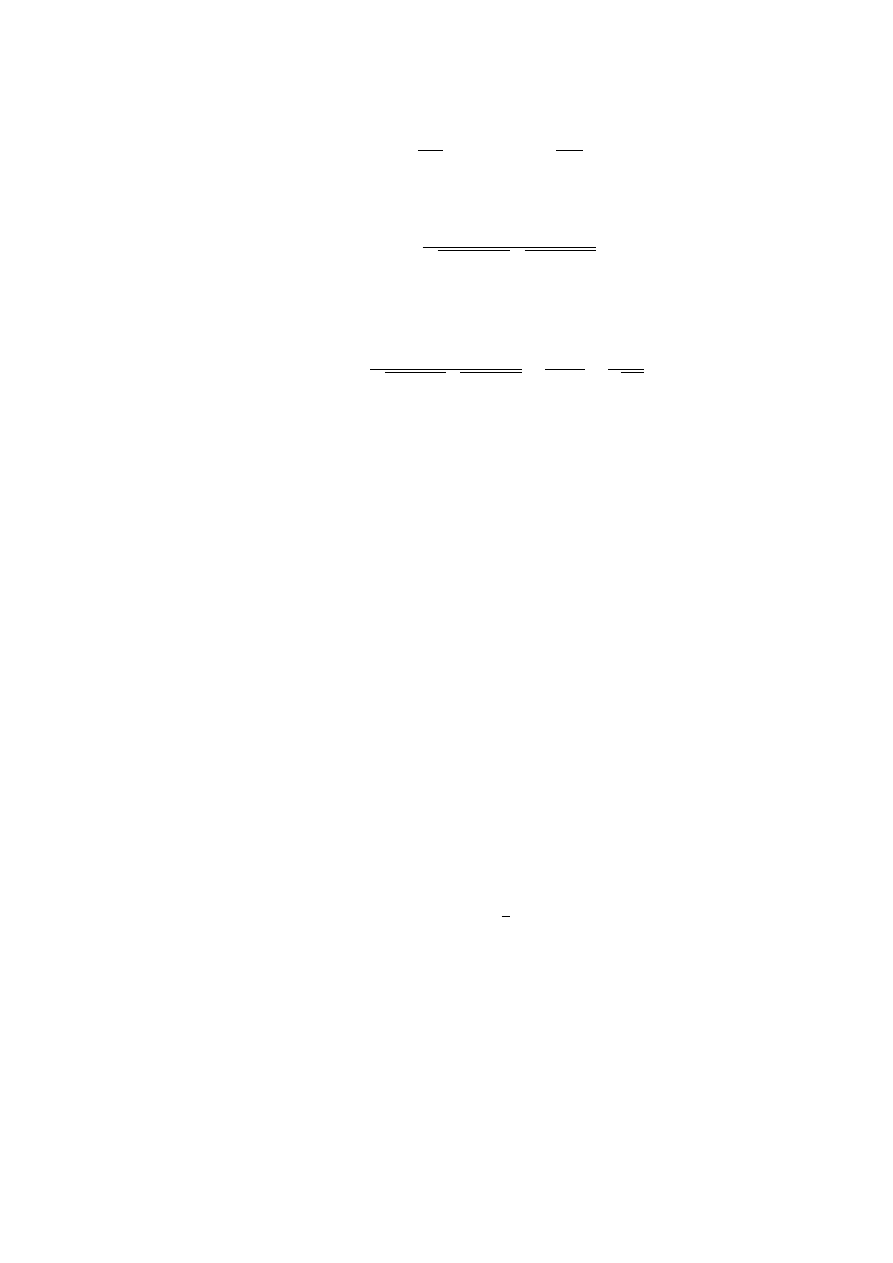
4.2. THE FIRST FUNDAMENTAL FORM
47
Let u
α
= φ
α
(t) and u
α
= ψ
α
(t) be two curves on the surface. Then the total differentials
du
α
=
dφ
α
dt
dt, and δu
α
=
dψ
α
dt
δt
represent infinitesimal tangent vectors (1.12) to the curves. Thus, the angle between two infinitesimal
vectors tangent to two intersecting curves on the surface satisfies the equation:
cos θ =
g
αβ
du
α
δu
β
p
g
αβ
du
α
du
β
p
g
αβ
δu
α
δu
β
(4.12)
In particular, if the two curves happen to be the parametric curves, u
1
= constant and u
2
=
constant, then along one curve we have du
1
= 0, with du
2
arbitrary, and along the second δu
1
is
arbitrary and δu
2
= 0. In this case, the cosine of the angle subtended by the infinitesimal tangent
vectors reduces to:
cos θ =
g
12
δu
1
du
2
p
g
11
(δu
1
)
2
p
g
22
(du
2
)
2
=
g
12
g
11
g
22
=
F
√
EG
.
(4.13)
I follows immediately from the equation above that:
4.7 Proposition The parametric lines are orthogonal if F = 0.
4.8 Examples
a) Sphere
x = (a sin θ cos φ, a sin θ sin φ, a cos θ)
x
θ
= (a cos θ cos φ, a cos θ sin φ, −a sin θ)
x
φ
= (−a sin θ sin φ, a sin θ cos φ, 0)
E
= x
θ
· x
θ
= a
2
F
= x
θ
· x
φ
= 0
G = x
φ
· x
φ
= a
2
sin
2
θ
ds
2
= a
2
dθ
2
+ a
2
sin
2
θdφ
2
b) Surface of Revolution
x = (r cos θ, r sin θ, f (r))
x
r
= (cos θ, sin θ, f
0
(r))
x
θ
= (−r sin θ, r cos θ, 0)
E
= x
r
· x
r
= 1 + f
02
(r)
F
= x
r
· x
θ
= 0
G = x
θ
· x
θ
= r
2
ds
2
= [1 + f
02
(r)]dr
2
+ r
2
dθ
2
c) Pseudosphere
x = (a sin u cos v, a sin u sin v, a(cos u ln tan
u
2
))
E
= a
2
cot
2
u
F
= = 0
G = a
2
sin
2
u
ds
2
= a
2
cot
2
udu
2
+ a
2
sin
2
udv
2
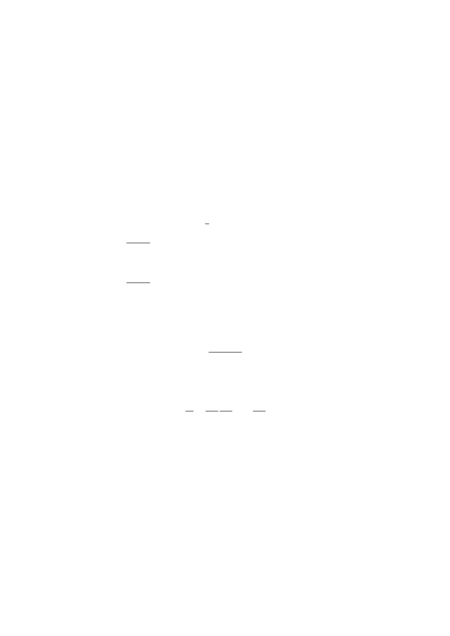
48
CHAPTER 4. THEORY OF SURFACES
d) Torus
x = ((b + a cos u) cos v, (b + a cos u) sin v, a sin u)
E
= a
2
F
= 0
G = (b + a cos u)
2
ds
2
= a
2
du
2
+ (b + a cos u)
2
dv
2
e) Helicoid
x = (u cos v, u sin v, av)
E
= 1
F
= 0
G = u
2
+ a
2
ds
2
= du
2
+ (u
2
+ a
2
)dv
2
f) Catenoid
x = (u cos v, u sin v, c cosh
−1
u
c
)
E
=
u
2
u
2
− c
2
F
= 0
G = u
2
ds
2
=
u
2
u
2
− c
2
du
2
+ u
2
dv
2
4.3
The Second Fundamental Form
Let x = x(u
α
) be a coordinate patch on a surface M. Since x
u
and x
v
are tangential to the surface,
we can construct a unit normal n to the surface by taking
n =
x
u
× x
v
kx
u
× x
v
k
(4.14)
Now, consider a curve on the surface given by u
α
= u
α
(s). Without loss of generality, we assume
that the curve is parametrized by arclength s so that the curve has unit speed. Using the chain rule,
we se that the unit tangent vector T to the curve is given by
T =
dx
ds
=
dx
du
α
du
α
ds
= x
α
du
α
ds
(4.15)
Since the curve lives on the surface and the the vector T is tangent to the curve, it is clear that
T is also tangent to the surface. On the other hand, the vector T
0
= dT /ds does not in general have
this property, so we decompose T
0
into its normal and tangential components (see fig. (4.2))
T
0
= K
n
+ K
g
= κ
n
n + K
g
,
(4.16)
where κ
n
= kK
n
k =< T
0
, n > .
The scalar quantity κ
n
is called the normal curvature of the curve and K
g
is called the
geodesic curvature vector. The normal curvature measures the the curvature of x(u
α
(s)) resulting
4.3. THE SECOND FUNDAMENTAL FORM
49
Figure not yet available.
Figure 4.2: Normal Curvature
from the constraint of the curve to lie on a surface. The geodesic curvature vector , measures the
“sideward” component of the curvature in the tangent plane to the surface. Thus, if one draws a
straight line on a flat piece of paper and then smoothly bends the paper into a surface, then the
straight line would now acquire some curvature. Since the line was originally straight, there is no
sideward component of curvature so K
g
= 0 in this case. This means that the entire contribution
to the curvature comes from the normal component, reflecting the fact that the only reason there is
curvature here is due to the bend in the surface itself.
Similarly, if one specifies a point p ∈ M and a direction vector X
p
∈ T
p
M, one can geometrically
envision the normal curvature by considering the equivalence class of all unit speed curves in M
that contain the point p and whose tangent vectors line up with the direction of X. Of course,
there are infinitely many such curves, but at an infinitesimal level, all these curves can be obtained
by intersecting the surface with a “vertical” plane containing the vector X and the normal to M.
All curves in this equivalence class have the same normal curvature and their geodesic curvatures
vanish. In this sense, the normal curvature is more of a property pertaining to a direction on the
surface at a point, whereas the geodesic curvature really depends on the curve itself. It might be
impossible for a hiker walking on the undulating hills of the Ozarks to find a straight line trail, since
the rolling hills of the terrain extend in all directions. It might be possible, however, for the hiker
to walk on a path with zero geodesic curvature as long the same compass direction is maintained.
To find an explicit formula for the normal curvature we first differentiate equation (4.15)
T
0
=
dT
ds
=
d
ds
(x
α
du
α
ds
)
=
d
ds
(x
α
)
du
α
ds
+ x
α
d
2
u
α
ds
2
= (
dx
α
du
β
du
β
ds
)
du
α
ds
+ x
α
d
2
u
α
ds
2
= x
αβ
du
α
ds
du
β
ds
+ x
α
d
2
u
α
ds
2
.
Taking the inner product of the last equation with the normal and noticing that < x
α
, n >= 0, we
get
κ
n
= < T
0
, n >=< x
αβ
, n >
du
α
ds
du
β
ds
=
b
αβ
du
α
du
β
g
αβ
du
α
du
β
,
(4.17)
where
b
αβ
=< x
αβ
, n >
(4.18)
4.9 Definition The expression
II = b
αβ
du
α
⊗ du
β
(4.19)

50
CHAPTER 4. THEORY OF SURFACES
is called the second fundamental form .
4.10 Proposition The second fundamental form is symmetric.
Proof: In the classical formulation of the second fundamental form, the proof is trivial. We have
b
αβ
= b
βα
, since for a C
∞
patch x(u
α
), we have x
αβ
= x
βα
, because the partial derivatives commute.
We will denote the coefficients of the second fundamental form as follows:
e = b
11
=< x
uu
, n >
f
= b
12
=< x
uv
, n >
= b
21
=< x
vu
, n >
g = b
22
=< x
vv
, n >,
so that equation (4.19) can be written as
II = edu
2
+ 2f dudv + gdv
2
,
(4.20)
and equation (4.17) as
κ
n
=
II
I
=
edu
2
+ 2f dudv + gdv
2
Edu
2
+ 2F dudv + Gdv
2
.
(4.21)
We would also like to point out that just as the first fundamental form can be represented as
I =< dx, dx >,
we can represent the second fundamental form as
II = − < dx, dn >
To see this, it suffices to note that differentiation of the identity, < x
α
, n >= 0, implies that
< x
αβ
, n >= − < x
α
, n
β
> .
Therefore,
< dx, dn > = < x
α
du
α
, n
β
du
β
>
= < x
α
du
α
, n
β
du
β
>
= < x
α
, n
β
> du
α
du
β
= − < x
αβ
, n > du
α
du
β
= −II
From a computational point a view, a more useful formula for the coefficients of the second
fundamental formula can be derived by first applying the classical vector identity
(A × B) · (C × D) =
¯
¯
¯
¯
A · C
A · D
B · C
B · D
¯
¯
¯
¯
(4.22)
to compute
kx
u
× x
v
k
2
= (x
u
× x
v
) · (x
u
× x
v
)
= det
·
x
u
· x
u
x
u
· x
v
x
v
· x
u
x
v
· x
v
¸
= EG − F
2
.
(4.23)
4.4. CURVATURE
51
Consequently, the normal vector can be written as
n =
x
u
× x
v
kx
u
× x
v
k
=
x
u
× x
v
√
EG − F
2
Thus, we can write the coefficients b
αβ
directly as triple products involving derivatives of (x). The
expressions for these coefficients are
e =
(x
u
x
u
x
uu
)
√
EG − F
2
f
=
(x
u
x
v
x
uv
)
√
EG − F
2
g =
(x
v
x
v
x
vv
)
√
EG − F
2
(4.24)
The first fundamental form on a surface measures the square of the distance between two in-
finitesimally separated points. There is a similar interpretation of the second fundamental form as
we show below. The second fundamental form measures the distance from a point on the surface
to the tangent plane at a second infinitesimally separated point. To see this simple geometrical
interpretation, consider a point x
0
= x(u
α
0
) ∈ M and a nearby point x(u
α
0
+ du
α
). Expanding on a
Taylor series, we get
x(u
α
0
+ du
α
) = x
0
+ (x
0
)
α
du
α
+
1
2
(x
0
)
αβ
du
α
du
β
+ . . . .
We recall that the distance formula from a point x to a plane which contains x
0
is just the scalar
projection of (x − x
0
) onto the normal. Since the normal to the plane at x
0
is the same as the unit
normal to the surface and < x
α
, n >= 0, we find that the distance D is
D = < x − x
0
, n >
=
1
2
< (x
0
)
αβ
, n > du
α
du
β
=
1
2
II
0
The first fundamental form (or, rather, its determinant) also appears in calculus in the context
of calculating the area of a parametrized surface. If one considers an infinitesimal parallelogram
subtended by the vectors x
u
du and x
v
dv, then the differential of surface area is given by the length
of the cross product of these two infinitesimal tangent vectors. That is,
dS
= kx
u
× x
v
k dudv
S
=
Z Z p
EG − F
2
dudv
The second fundamental form contains information about the shape of the surface at a point.
For example, the discussion above indicates that if b = |b
αβ
| = eg − f
2
> 0 then all the neighboring
points lie on the same side of the tangent plane, and hence, the surface is concave in one direction.
If at a point on a surface b > 0, the point is called an elliptic point, if b < 0, the point is called
hyperbolic or a saddle point, and if b = 0, the point is called parabolic.
4.4
Curvature
The concept of Curvature and its related, constitute the central object of study in differential
geometry. One would like to be able to answer questions such as “what quantities remain invariant
52
CHAPTER 4. THEORY OF SURFACES
as one surface is smoothly changed into another?” There is certainly something intrinsically different
between a cone, which we can construct from a flat piece of paper, and a sphere, which we cannot.
What is it that makes these two surfaces so different? How does one calculate the shortest path
between two objects when the path is constrained to lie on a surface?
These and questions of similar type can be quantitatively answered through the study of curva-
ture. We cannot overstate the importance of this subject; perhaps it suffices to say that, without a
clear understanding of curvature, there would be no general theory of relativity, no concept of black
holes, and even more disastrous, no Star Trek.
Studying the curvature of a hypersurface in R
n
(a surface of dimension n − 1) begins by trying
to understand the covariant derivative of the normal to the surface. If the normal to a surface
is constant, then the surface is a flat hyperplane. Variations in the normal are what indicates
the presence of curvature. For simplicity, we constrain our discussion to surfaces in R
3
, but the
formalism we use is applicable to any dimension. We will also introduce in the modern version of
the second fundamental form
4.11 Definition Let X be a vector field on a surface M in R
3
, and let N be the normal vector.
The map L, given by
LX = −∇
X
N
(4.25)
is called the Weingarten map.
In this definition we will be careful to differentiate operators that live on the surface from oper-
ators that live in the ambient space. We will adopt the convention of overlining objects that live in
the ambient space, the operator ∇ being an example of one such object. The Weingarten map is a
good place to start, since it represents the rate of change of the normal in an arbitrary direction we
wish to quantify.
4.12 Definition The Lie bracket [X, Y ] of two vector fields X and Y on a surface M is defined
as the commutator,
[X, Y ] = XY − Y X,
(4.26)
meaning that if f is a function on M, then [X, Y ](f ) = X(Y (f )) − Y (X(f )).
4.13 Proposition The Lie bracket of two vectors X, Y ∈ T (M) is another vector in T (M).
Proof:
If suffices to prove that the bracket is a linear derivation on the space of C
∞
functions.
Consider vectors X, Y ∈ T (M) and smooth functions f, g in M. Then,
[X, Y ](f + g) = X(Y (f + g)) − Y (X(f + g))
= X(Y (f ) + Y (g)) − Y (X(f ) + X(g))
= X(Y (f )) − Y (X(f )) + X(Y (g)) − Y (X(g))
= [X, Y ](f ) + [X, Y ](g),
and
[X, Y ](f g) = X(Y (f g)) − Y (X(f g))
= X[f Y (g) + gY (f )] − Y [f X(g) + gX(f )]
= X(f )Y (g) + f X(Y (g)) + X(g)Y (f ) + gX(Y (f ))
−Y (f )X(g) − f (Y (X(g)) − Y (g)X(f ) − gY (X(f ))
= f [X(Y (g)) − (Y (X(g))] + g[X(Y (f )) − Y (X(f ))]
= f [X, Y ](g) + g[X, Y ](f ).
4.4. CURVATURE
53
4.14 Proposition The Weingarten map is a linear transformation on T (M).
Proof:
Linearity follows from the linearity of ∇, so it suffices to show that L : X −→ LX maps
X ∈ T (M) to a vector LX ∈ T (M). Since N is the unit normal to the surface, < N, N >= 1, so
any derivative of < N, N > is 0. Assuming that the connection is compatible with the metric,
∇
X
< N, N > = < ∇
X
N, > + < N, ∇
X
N >
= 2 < ∇
X
N, N >
= 2 < LX, N >= 0.
Therefore, LX is orthogonal to N ; hence, it lies in T (M).
In the previous section, we gave two equivalent definitions < dx, dx >, and < X, Y >) of the
first fundamental form. We will now do the same for the second fundamental form.
4.15 Definition The second fundamental form is the bilinear map
II(X, Y ) =< LX, Y > .
(4.27)
4.16 Remark It should be noted that the two definitions of the second fundamental form are
consistent. This is easy to see if one chooses X to have components x
α
and Y to have components
x
β
. With these choices, LX has components −n
a
and II(X, Y ) becomes b
αβ
= − < x
α
, n
β
>.
We also note that there is a third fundamental form defined by
III(X, Y ) =< LX, LY >=< L
2
X, Y > .
(4.28)
In classical notation, the third fundamental form would be denoted by < dn, dn >. As one would
expect, the third fundamental form contains third order Taylor series information about the surface.
We will not treat III(X, Y ) in much detail in this work.
4.17 Definition The torsion of a connection ∇ is the operator T such that ∀X, Y,
T (X, Y ) = ∇
X
Y − ∇
Y
X − [X, Y ].
(4.29)
A connection is called torsion-free if T (X, Y ) = 0. In this case,
∇
X
Y − ∇
Y
X = [X, Y ].
We will say more later about the torsion and the importance of torsion-free connections. For
the time being, it suffices to assume that for the rest of this section, all connections are torsion-free.
Using this assumption, it is possible to prove the following important theorem.
4.18 Theorem The Weingarten map is a self-adjoint operator on T M.
Proof: We have already shown that L : T M −→ T M is a linear map. Recall that an operator L
on a linear space is self adjoint if < LX, Y >=< X, LY >, so the theorem is equivalent to proving
that the second fundamental form is symmetric (II[X, Y ] = II[Y, X]). Computing the difference of
these two quantities, we get
II[X, Y ] − II[Y, X] = < LX, Y > − < LY, X >
= < ∇
X
N, Y > − < ∇
Y
N, X > .
Since < X, N >=< Y, N >= 0 and the connection is compatible with the metric, we know that
< ∇
X
N, Y > = − < N, ∇
X
Y >
< ∇
Y
N, X > = − < N, ∇
Y
X >,
54
CHAPTER 4. THEORY OF SURFACES
hence,
II[X, Y ] − II[Y, X] = < N, ∇
Y
X > − < N, ∇
X
Y >,
= < N, ∇
Y
X − ∇
X
Y >
= < N, [X, Y ] >
= 0
(iff [X, Y ] ∈ T (M)).
The central theorem of linear algebra is the Spectral Theorem. In the case of self-adjoint opera-
tors, the Spectral Theorem states that given the eigenvalue equation for a symmetric operator on a
vector space with an inner product,
LX = κX,
(4.30)
the eigenvalues are always real and eigenvectors corresponding to different eigenvalues are orthogonal.
Here, the vector spaces in question are the tangent spaces at each point of a surface in R
3
, so the
dimension is 2. Hence, we expect two eigenvalues and two eigenvectors:
LX
1
= κ
1
X
1
(4.31)
LX
2
= κ
1
X
2
.
(4.32)
4.19 Definition The eigenvalues κ
1
and κ
2
of the Weingarten map L are called the principal
curvatures and the eigenvectors X
1
and X
2
are called the principal directions.
Several possible situations may occur, depending on the classification of the eigenvalues at each
point p on a given surface:
1. If κ
1
6= κ
2
and both eigenvalues are positive, then p is called an elliptic point.
2. If κ
1
κ
2
< 0, then p is called a hyperbolic point.
3. If κ
1
= κ
2
6= 0, then p is called an umbilic point.
4. If κ
1
κ
2
= 0, then p is called a parabolic point.
It is also known from linear algebra, that the the determinant and the trace of a self-adjoint
operator in a vector space of dimension two are the only invariants under a adjoint (similarity)
transformation. Clearly, these invariants are important in the case of the operator L, and they
deserve special names.
4.20 Definition The determinant K = det(L) is called the Gaussian curvature of M and
H = (1/2)Tr(L) is called the mean curvature.
Since any self-adjoint operator is diagonalizable and in a diagonal basis the matrix representing
L is diag(κ
1
, κ
2
), if follows immediately that
K
= κ
1
κ
2
H
=
1
2
(κ
1
+ κ
2
).
(4.33)
4.21 Proposition Let X and Y be any linearly independent vectors in T (M). Then
LX × LY
= K(X × Y )
(LX × Y ) + (X × LY ) = 2H(X × Y )
(4.34)
Proof: Since LX, LY ∈ T (M), they can be expressed as linear combinations of the basis vectors
X and Y .

4.4. CURVATURE
55
LX
= a
1
X + b
1
Y
LY
= a
2
X + b
2
Y.
computing the cross product, we get
LX × LY
=
¯
¯
¯
¯
a
1
b
1
a
2
b
2
¯
¯
¯
¯ X × Y
= det(L)(X × Y ).
Similarly
(LX × Y ) + (X × LY ) = (a
1
+ b
2
)(X × Y )
= Tr(L)(X × Y )
= (2H)(X × Y ).
4.22 Proposition
K
=
eg − f
2
EG − F
2
H
=
1
2
Eg − 2F f + eG
EG − F
2
(4.35)
Proof:
Starting with equations (4.34), take the inner product of both sides with X × Y and use
the vector identity (4.22). We immediately get
K =
¯
¯
¯
¯
< LX, X >
< LX, Y >
< LY, X >
< LX, X >
¯
¯
¯
¯
¯
¯
¯
¯
< X, X > < X, Y >
< Y, X >
< Y, Y >
¯
¯
¯
¯
2H =
¯
¯
¯
¯
< LX, X > < LX, Y >
< Y, X >
< Y, Y >
¯
¯
¯
¯ +
¯
¯
¯
¯
< X, X >
< X, Y >
< LY, X > < LY, Y >
¯
¯
¯
¯
¯
¯
¯
¯
< X, X > < X, Y >
< Y, X >
< Y, Y >
¯
¯
¯
¯
The result follows by taking X = x
u
and Y = x
v
4.23 Theorem (Euler) Let X
1
and X
2
be unit eigenvectors of L and let X = (cos θ)X
1
+(sin θ)X
2
.
Then
II(X, X) = κ
1
cos
2
θ + κ
2
sin
2
θ.
(4.36)
Proof:
Simply compute II(X, X) =< LX, X >, using the fact the LX
1
= κ
1
X
1
, LX
2
= κ
2
X
2
,
and noting that the eigenvectors are orthogonal. We get
< LX, X > = < (cos θ)κ
1
X
1
+ (sin θ)κ
2
X
2
, (cos θ)X
1
+ (sin θ)X
2
>
= κ
1
cos
2
θ < X
1
, X
1
> +κ
2
sin
2
θ < X
2
, X
2
>
= κ
1
cos
2
θ + κ
2
sin
2
θ.
Wyszukiwarka
Podobne podstrony:
Gardner Differential geometry and relativity (lecture notes, web draft, 2004) (198s) PGr
Rajeev S G Geometrical methods in physics (lecture notes, web draft, 2004)(97s)
Freitag Several complex variables local theory (lecture notes, web draft, 2001)(74s) MCc
Rajeev S G Advanced classical mechanics chaos (Rochester lecture notes, web draft, 2002)(100s) PCtm
Walet N Further Maths 2C1 Lecture Notes(web draft, 2002)(79s) MCde
Gudmundsson S An introduction to Riemannian geometry(web draft, 2006)(94s) MDdg
Dahl M A brief introduction to Finsler geometry (web draft, 2006)(39s) MDdg (1)
Differential Geometry in Physics, 3 of 4 (Gabriel Lugo)
Differential Geometry in Physics, 2 of 4 (Gabriel Lugo)
Differential Geometry in Physics, 1 of 4 (Gabriel Lugo)
Differential Geometry in Physics, 4 of 4 (Gabriel Lugo)
Corporate Identity Image and Brands lecture notes
Introduction to Differential Geometry and General Relativity
Athanassopoulos K Notes on symplectic geometry (Univ of Crete, web draft, 2007)(66s) MDdg
Gray R M Toeplitz and circulant matrices a review (web draft, 2005)(89s) MAl
Hitchin N Differentiable manifolds (web draft, 2003)(92s) MDdg
Black T H Derivations of applied mathematics (web draft, 2006)(246s) MCet
Neumann W D Notes on geometry and 3 manifolds, with appendices by P Norbury (web draft, 2004)(54s)
więcej podobnych podstron