

2

2C1:
Further Mathematical Methods
Niels Walet, Fall 2002
Version: October 23, 2002
Copyright by Niels R. Walet, Dept of Physics, UMIST
Copying for personal or study use permitted
Copying for commercial use or profit disallowed

4

Contents
1 Introduction
7
1.1
Ordinary differential equations . . . . . . . . . . . . . . . . . . . . . . . . . . . . . . . . . . . .
7
1.2
PDE’s . . . . . . . . . . . . . . . . . . . . . . . . . . . . . . . . . . . . . . . . . . . . . . . . . .
7
2 Classification of partial differential equations.
11
3 Boundary and Initial Conditions
15
3.1
Explicit boundary conditions . . . . . . . . . . . . . . . . . . . . . . . . . . . . . . . . . . . . .
16
3.1.1
Dirichlet boundary condition . . . . . . . . . . . . . . . . . . . . . . . . . . . . . . . . .
16
3.1.2
von Neumann boundary conditions . . . . . . . . . . . . . . . . . . . . . . . . . . . . . .
16
3.1.3
Mixed (Robin’s) boundary conditions . . . . . . . . . . . . . . . . . . . . . . . . . . . .
17
3.2
Implicit boundary conditions . . . . . . . . . . . . . . . . . . . . . . . . . . . . . . . . . . . . .
17
3.3
A slightly more realistic example . . . . . . . . . . . . . . . . . . . . . . . . . . . . . . . . . . .
17
3.3.1
A string with fixed endpoints . . . . . . . . . . . . . . . . . . . . . . . . . . . . . . . . .
17
3.3.2
A string with freely floating endpoints . . . . . . . . . . . . . . . . . . . . . . . . . . . .
17
3.3.3
A string with endpoints fixed to strings . . . . . . . . . . . . . . . . . . . . . . . . . . .
18
4 Fourier Series
21
4.1
Taylor series . . . . . . . . . . . . . . . . . . . . . . . . . . . . . . . . . . . . . . . . . . . . . . .
21
4.2
Introduction to Fourier Series . . . . . . . . . . . . . . . . . . . . . . . . . . . . . . . . . . . . .
21
4.3
Periodic functions
. . . . . . . . . . . . . . . . . . . . . . . . . . . . . . . . . . . . . . . . . . .
22
4.4
Orthogonality and normalisation . . . . . . . . . . . . . . . . . . . . . . . . . . . . . . . . . . .
22
4.5
When is it a Fourier series? . . . . . . . . . . . . . . . . . . . . . . . . . . . . . . . . . . . . . .
23
4.6
Fourier series for even and odd functions . . . . . . . . . . . . . . . . . . . . . . . . . . . . . . .
25
4.7
Convergence of Fourier series . . . . . . . . . . . . . . . . . . . . . . . . . . . . . . . . . . . . .
26
5 Separation of variables on rectangular domains
29
5.1
Cookbook . . . . . . . . . . . . . . . . . . . . . . . . . . . . . . . . . . . . . . . . . . . . . . . .
29
5.2
parabolic equation . . . . . . . . . . . . . . . . . . . . . . . . . . . . . . . . . . . . . . . . . . .
30
5.3
hyperbolic equation . . . . . . . . . . . . . . . . . . . . . . . . . . . . . . . . . . . . . . . . . . .
31
5.4
Laplace’s equation . . . . . . . . . . . . . . . . . . . . . . . . . . . . . . . . . . . . . . . . . . .
33
5.5
More complex initial/boundary conditions . . . . . . . . . . . . . . . . . . . . . . . . . . . . . .
34
5.6
Inhomogeneous equations . . . . . . . . . . . . . . . . . . . . . . . . . . . . . . . . . . . . . . .
36
6 D’Alembert’s solution to the wave equation
39
7 Polar and spherical coordinate systems
45
7.1
Polar coordinates . . . . . . . . . . . . . . . . . . . . . . . . . . . . . . . . . . . . . . . . . . . .
45
7.2
spherical coordinates . . . . . . . . . . . . . . . . . . . . . . . . . . . . . . . . . . . . . . . . . .
46
8 Separation of variables in polar coordinates
51
5

6
CONTENTS
9 Series solutions of O.D.E.
55
9.1
Singular points . . . . . . . . . . . . . . . . . . . . . . . . . . . . . . . . . . . . . . . . . . . . .
56
9.2
*Special cases . . . . . . . . . . . . . . . . . . . . . . . . . . . . . . . . . . . . . . . . . . . . . .
57
9.2.1
Two equal roots . . . . . . . . . . . . . . . . . . . . . . . . . . . . . . . . . . . . . . . .
57
9.2.2
Two roots differing by an integer . . . . . . . . . . . . . . . . . . . . . . . . . . . . . . .
57
9.2.3
Example 1 . . . . . . . . . . . . . . . . . . . . . . . . . . . . . . . . . . . . . . . . . . . .
58
9.2.4
Example 2 . . . . . . . . . . . . . . . . . . . . . . . . . . . . . . . . . . . . . . . . . . . .
59
10 Bessel functions
61
10.1 Temperature on a disk . . . . . . . . . . . . . . . . . . . . . . . . . . . . . . . . . . . . . . . . .
61
10.2 Bessel’s equation . . . . . . . . . . . . . . . . . . . . . . . . . . . . . . . . . . . . . . . . . . . .
62
10.3 Gamma function . . . . . . . . . . . . . . . . . . . . . . . . . . . . . . . . . . . . . . . . . . . .
64
10.4 Bessel functions of general order . . . . . . . . . . . . . . . . . . . . . . . . . . . . . . . . . . .
65
10.5 Properties of Bessel functions . . . . . . . . . . . . . . . . . . . . . . . . . . . . . . . . . . . . .
66
10.6 Sturm-Liouville theory . . . . . . . . . . . . . . . . . . . . . . . . . . . . . . . . . . . . . . . . .
67
10.7 Our initial problem and Bessel functions . . . . . . . . . . . . . . . . . . . . . . . . . . . . . . .
69
10.8 Fourier-Bessel series . . . . . . . . . . . . . . . . . . . . . . . . . . . . . . . . . . . . . . . . . .
70
10.9 Back to our initial problem . . . . . . . . . . . . . . . . . . . . . . . . . . . . . . . . . . . . . .
72
11 Separation of variables in three dimensions
73
11.1 Modelling the eye . . . . . . . . . . . . . . . . . . . . . . . . . . . . . . . . . . . . . . . . . . . .
73
11.2 Properties of Legendre polynomials . . . . . . . . . . . . . . . . . . . . . . . . . . . . . . . . . .
75
11.2.1 Generating function . . . . . . . . . . . . . . . . . . . . . . . . . . . . . . . . . . . . . .
75
11.2.2 Rodrigues’ Formula . . . . . . . . . . . . . . . . . . . . . . . . . . . . . . . . . . . . . .
76
11.2.3 A table of properties . . . . . . . . . . . . . . . . . . . . . . . . . . . . . . . . . . . . . .
76
11.3 Fourier-Legendre series . . . . . . . . . . . . . . . . . . . . . . . . . . . . . . . . . . . . . . . . .
77
11.4 Modelling the eye–revisited . . . . . . . . . . . . . . . . . . . . . . . . . . . . . . . . . . . . . .
78

Chapter 1
Introduction
In this course we shall consider so-called linear Partial Differential Equations (P.D.E.’s). This chapter is
intended to give a short definition of such equations, and a few of their properties. However, before introducing
a new set of definitions, let me remind you of the so-called ordinary differential equations (O.D.E.’s) you have
encountered in many physical problems.
1.1
Ordinary differential equations
ODE’s are equations involving an unknown function and its derivatives, where the function depends on a single
variable, e.g., the equation for a particle moving at constant velocity,
d
dt
x(t) = v,
(1.1)
which has the well known solution
x(t) = vt + x
0
.
(1.2)
The unknown constant x
0
is called an integration constant, and can be determined if we know where the
particle is located at time t = 0. If we go to a second order equation (i.e., one containing the second derivative
of the unknown function), we find more integration constants: the harmonic oscillator equation
d
2
dt
2
x(t) = −ω
2
x(t)
(1.3)
has as solution
x = A cos ωt + B sin ωt,
(1.4)
which contains two constants.
As we can see from the simple examples, and as you well know from experience, these equations are
relatively straightforward to solve in general form. We need to know only the coordinate and position at one
time to fix all constants.
1.2
PDE’s
Rather than giving a strict mathematical definition, let us look at an example of a PDE, the heat equation in
1 space dimension
∂
2
u(x, t)
∂x
2
=
1
k
∂u(x, t)
∂t
.
(1.5)
• It is a PDE since partial derivatives are involved.
7

8
CHAPTER 1. INTRODUCTION
To remind you of what that means:
∂u(x,t)
∂x
denotes the differentiation of u(x, t) w.r.t. x
keeping t fixed,
∂(x
2
t + xt
2
)
∂x
= 2xt + t
2
.
(1.6)
• It is called linear since u and its derivatives appear linearly, i.e., once per term. No functions of u are
allowed. Terms like u
2
, sin(u), u
∂u
∂x
, etc., break this rule, and lead to non-linear equations. These are
interesting and important in their own right, but outside the scope of this course.
• Equation (1.5) above is also homogeneous (which just means that every term involves either u or one of
its derivatives, there is no term that does not contain u). The equation
∂
2
u(x, t)
∂x
2
=
1
k
∂u(x, t)
∂t
+ sin(x)
(1.7)
is called inhomogeneous, due to the sin(x) term on the right, that is independent of u.
Why is all that so important? A linear homogeneous equation allows superposition of
solutions. If u
1
and u
2
are both solutions to the heat equation,
∂
2
u
1
(x, t)
∂x
2
−
1
k
∂u
1
(x, t)
∂t
=
∂
2
u
2
(x, t)
∂x
2
−
1
k
∂u
2
(x, t)
∂t
= 0,
(1.8)
any combination is also a solution,
∂
2
[au
1
(x, t) + bu
2
(x, t)]
∂x
2
−
1
k
∂[au
1
(x, t) + bu
2
(x, t)]
∂t
= 0.
(1.9)
For a linear inhomogeneous equation this gets somewhat modified. Let v be any solution
to the heat equation with a sin(x) inhomogeneity,
∂
2
v(x, t)
∂x
2
−
1
k
∂v(x, t)
∂t
= sin(x).
(1.10)
In that case v + au
1
, with u
1
a solution to the homogeneous equation, see Eq. (1.8), is also
a solution,
∂
2
[v(x, t) + au
1
(x, t)]
∂x
2
−
1
k
∂[v(x, t) + au
1
(x, t)]
∂t
=
∂
2
v(x, t)
∂x
2
−
1
k
∂v(x, t)
∂t
+ a
∂
2
u
1
(x, t)
∂x
2
−
1
k
∂u
1
(x, t)
∂t
= sin(x).
(1.11)
Finally we would like to define the order of a PDE as the power in the highest derivative, even it is a mixed
derivative (w.r.t. more than one variable).
Quiz
Which of these equations is linear? and which is homogeneous?
a)
∂
2
u
∂x
2
+ x
2
∂u
∂y
= x
2
+ y
2
.
(1.12)
b)
y
2
∂
2
u
∂x
2
+ u
∂u
∂x
+ x
2
∂
2
u
∂y
2
= 0.
(1.13)

1.2. PDE’S
9
c)
∂u
∂x
2
+
∂
2
u
∂y
2
= 0.
(1.14)
What is the order of the following equations?
a)
∂
3
u
∂x
3
+
∂
2
u
∂y
2
= 0.
(1.15)
b)
∂
2
u
∂x
2
− 2
∂
4
u
∂x
3
∂y
+
∂
2
u
∂y
2
= 0.
(1.16)

10
CHAPTER 1. INTRODUCTION

Chapter 2
Classification of partial differential
equations.
Partial differential equations occur in many different areas of physics, chemistry and engineering. Let me give
a few examples, with their physical context. Here, as is common practice, I shall write ∇
2
to denote the sum
∇
2
=
∂
2
∂x
2
+
∂
2
∂y
2
+ . . .
(2.1)
• The wave equation, ∇
2
u =
1
c
2
∂
2
u
∂t
2
.
This can be used to describes the motion of a string or drumhead (u is vertical displacement), as well as
a variety of other waves (sound, light, ...). The quantity c is the speed of wave propagation.
• The heat or diffusion equation, ∇
2
u =
1
k
∂u
∂t
.
This can be used to describe the change in temperature (u) in a system conducting heat, or the diffusion
of one substance in another (u is concentration). The quantity k, sometimes replaced by a
2
, is the
diffusion constant, or the heat capacity. Notice the irreversible nature: If t → −t the wave equation
turns into itself, but not the diffusion equation.
• Laplace’s equation ∇
2
u = 0.
• Helmholtz’s equation ∇
2
u + λu = 0.
This occurs for waves in wave guides, when searching for eigenmodes (resonances).
• Poisson’s equation ∇
2
u = f (x, y, . . .).
The equation for the gravitational field inside a gravitational body, or the electric field inside a charged
sphere.
• Time-independent Schr¨odinger equation, ∇
2
u =
2m
~
2
[E − V (x, y, . . .)]u = 0.
|u|
2
has a probability interpretation.
• Klein-Gordon equation ∇
2
u −
1
c
2
∂
2
u
∂t
2
+ λ
2
u = 0.
Relativistic quantum particles,
|u|
2
has a probability interpretation.
These are all second order differential equations. (Remember that the order is defined as the highest
derivative appearing in the equation.)
11

12
CHAPTER 2. CLASSIFICATION OF PARTIAL DIFFERENTIAL EQUATIONS.
Second order P.D.E. are usually divided into three types. Let me show this for two-dimensional PDE’s:
a
∂
2
u
∂x
2
+ 2c
∂
2
u
∂x∂y
+ b
∂
2
u
∂y
2
+ d
∂u
∂x
+ e
∂u
∂y
+ f u + g = 0
(2.2)
where a, . . . , g can either be constants or given functions of x, y. If g is 0 the system is called homogeneous,
otherwise it is called inhomogeneous. Now the differential equation is said to be
elliptic
hyperbolic
parabolic
if ∆(x, y) = ab − c
2
is
positive
negative
zero
(2.3)
Why do we use these names? The idea is most easily explained for a case with constant coefficients, and
correspond to a classification of the associated quadratic form (replace derivative w.r.t. x and y with ξ and η)
aξ
2
+ bη
2
+ 2cξη + f = 0.
(2.4)
We neglect d and e since they only describe a shift of the origin. Such a quadratic equation can describe any
of the geometrical figures discussed above. Let me show an example, a = 3, b = 3, c = 1 and f =
−3. Since
ab − c
2
= 8, this should describe an ellipse. We can write
3ξ
2
+ 3η
2
+ 2ξη = 4(
ξ + η
√
2
)
2
+ 2(
ξ − η
√
2
)
2
= 3,
(2.5)
which is indeed the equation of an ellipse, with rotated axes, as can be seen in Fig. 2.1,
−1
0
1
ξ
−1
0
1
η
Figure 2.1: The ellipse corresponding to Eq. (2.5)
We should also realize that Eq. (2.5) can be written in the vector-matrix-vector form
(ξ, η)
3 1
1 3
ξ
η
= 3.
(2.6)
We now recognise that ∆ is nothing more than the determinant of this matrix, and it is positive if both
eigenvalues are equal, negative if they differ in sign, and zero if one of them is zero. (Note: the simplest ellipse
corresponds to x
2
+ y
2
= 1, a parabola to y = x
2
, and a hyperbola to x
2
− y
2
= 1)
Quiz
What is the order of the following equations

13
a
∂
3
u
∂x
3
+
∂
2
u
∂y
2
= 0
(2.7)
b
∂
2
u
∂x
2
− 2
∂
4
u
∂x
3
u
+
∂
2
u
∂y
2
= 0
(2.8)
Classify the following differential equations (as elliptic, etc.)
a
∂
2
u
∂x
2
− 2
∂
2
u
∂x∂y
+
∂
2
u
∂y
2
= 0
b
∂
2
u
∂x
2
+
∂
2
u
∂y
2
+
∂u
∂x
= 0
c
∂
2
u
∂x
2
−
∂
2
u
∂y
2
+ 2
∂u
∂x
= 0
d
∂
2
u
∂x
2
+
∂u
∂x
+ 2
∂u
∂y
= 0
d
y
∂
2
u
∂x
2
+ x
∂
2
u
∂y
2
= 0
In more than two dimensions we use a similar definition, based on the fact that all eigenvalues of the
coefficient matrix have the same sign (for an elliptic equation), have different signs (hyperbolic) or one of them
is zero (parabolic). This has to do with the behaviour along the characteristics, as discussed below.
Let me give a slightly more complex example
x
2
∂
2
u
∂x
2
+ y
2
∂
2
u
∂y
2
+ z
2
∂
2
u
∂z
2
+ 2xy
∂
2
u
∂x∂y
+ 2xz
∂
2
u
∂x∂z
+ 2yz
∂
2
u
∂y∂z
= 0.
(2.9)
The matrix associated with this equation is
x
2
xy
xz
xy
y
2
yz
xz
yz
z
2
(2.10)
If we evaluate its characteristic polynomial we find that it is
λ
2
(x
2
− y
2
+ z
2
− λ) = 0.
(2.11)
Since this has always (for all x, y, z) two zero eigenvalues this is a parabolic differential equation.
Characteristics and classification A key point for classifying the equations this way is
not that we like the conic sections so much, but that the equations behave in very different
ways if we look at the three different cases. Pick the simplest representative case for each
class:
(2.12)

14
CHAPTER 2. CLASSIFICATION OF PARTIAL DIFFERENTIAL EQUATIONS.

Chapter 3
Boundary and Initial Conditions
As you all know, solutions to ordinary differential equations are usually not unique (integration constants
appear in many places). This is of course equally a problem for PDE’s. PDE’s are usually specified through
a set of boundary or initial conditions. A boundary condition expresses the behaviour of a function on the
boundary (border) of its area of definition. An initial condition is like a boundary condition, but then for the
time-direction. Not all boundary conditions allow for solutions, but usually the physics suggests what makes
sense. Let me remind you of the situation for ordinary differential equations, one you should all be familiar
with, a particle under the influence of a constant force,
d
2
x
dt
2
= a.
(3.1)
Which leads to
dx
dt
= at + v
0
,
(3.2)
and
x =
1
2
at
2
+ v
0
t + x
0
.
(3.3)
This contains two integration constants. Standard practice would be to specify
∂x
∂t
(t = 0) = v
0
and x(t = 0) =
x
0
. These are linear initial conditions (linear since they only involve x and its derivatives linearly), which
have at most a first derivative in them. This one order difference between boundary condition and equation
persists to PDE’s. It is kind of obviously that since the equation already involves that derivative, we can not
specify the same derivative in a different equation.
The important difference between the arbitrariness of integration constants in PDE’s and ODE’s is that
whereas solutions of ODE’s these are really constants, solutions of PDE’s contain arbitrary functions.
Let me give an example. Take
u = yf (x)
(3.4)
then
∂u
∂y
= f (x).
(3.5)
This can be used to eliminate f from the first of the equations, giving
u = y
∂u
∂y
(3.6)
which has the general solution u = yf (x).
15
16
CHAPTER 3. BOUNDARY AND INITIAL CONDITIONS
One can construct more complicated examples. Consider
u(x, y) = f (x + y) + g(x − y)
(3.7)
which gives on double differentiation
∂
2
u
∂x
2
−
∂
2
u
∂y
2
= 0.
(3.8)
The problem is that without additional conditions the arbitrariness in the solutions makes it almost useless
(if possible) to write down the general solution. We need additional conditions, that reduce this freedom. In
most physical problems these are boundary conditions, that describes how the system behaves on its boundaries
(for all times) and initial conditions, that specify the state of the system for an initial time t = 0. In the ODE
problem discussed before we have two initial conditions (velocity and position at time t = 0).
3.1
Explicit boundary conditions
For the problems of interest here we shall only consider linear boundary conditions, which express a linear
relation between the function and its partial derivatives, e.g.,
u(x, y = 0) + x
∂u
∂x
(x, y = 0) = 0.
(3.9)
As before the maximal order of the derivative in the boundary condition is one order lower than the order of
the PDE. For a second order differential equation we have three possible types of boundary condition
3.1.1
Dirichlet boundary condition
When we specify the value of u on the boundary, we speak of Dirichlet boundary conditions. An example for
a vibrating string with its ends, at x = 0 and x = L, fixed would be
u(0, t) = u(L, t) = 0.
(3.10)
3.1.2
von Neumann boundary conditions
In multidimensional problems the derivative of a function w.r.t. to each of the variables forms a vector field
(i.e., a function that takes a vector value at each point of space), usually called the gradient. For three variables
this takes the form
gradf (x, y, z) = ∇f(x, y, z) =
∂f
∂x
(x, y, z),
∂f
∂y
(x, y, z),
∂f
∂z
(x, y, z)
.
(3.11)
normal
gradient
boundary
Figure 3.1: A sketch of the normal derivatives used in the von Neumann boundary conditions.
Typically we cannot specify the gradient at the boundary, since that is too restrictive to allow for solutions.
We can – and in physical problems often need to – specify the component normal to the boundary, see Fig.
3.1 for an example. When this normal derivative is specified we speak of von Neumann boundary conditions.
3.2. IMPLICIT BOUNDARY CONDITIONS
17
In the case of an insulated (infinitely thin) rod of length a, we can not have a heat-flux beyond the ends
so that the gradient of the temperature must vanish (heat can only flow where a difference in temperature
exists). This leads to the BC
∂u
∂x
(0, t) =
∂u
∂x
(a, t) = 0.
(3.12)
3.1.3
Mixed (Robin’s) boundary conditions
We can of course mix Dirichlet and von Neumann boundary conditions. For the thin rod example given above
we could require
u(0, t) +
∂u
∂x
(0, t) = u(a, t) +
∂u
∂x
(a, t) = 0.
(3.13)
3.2
Implicit boundary conditions
In many physical problems we have implicit boundary conditions, which just mean that we have certain
conditions we wish to be satisfied. This is usually the case for systems defined on an infinite definition
area. For the case of the Schr¨
odinger equation this usually means that we require the wave function to be
normalisable. We thus have to disallow the wave function blowing up at infinity. Sometimes we implicitly
assume continuity or differentiability. In general one should be careful about such implicit BC’s, which may
be extremely important
3.3
A slightly more realistic example
3.3.1
A string with fixed endpoints
Consider a string fixed at x = 0 and x = a, as in Fig. 3.2
x=0
x=a
Figure 3.2: A string with fixed endpoints.
It satisfies the wave equation
1
c
2
∂
2
u
∂t
2
=
∂
2
u
∂x
2
,
0 < x < a,
(3.14)
with boundary conditions
u(0, t) = u(a, t) = 0,
t > 0,
(3.15)
and initial conditions,
u(x, 0) = f (x),
∂u
∂x
(x, 0) = g(x).
(3.16)
3.3.2
A string with freely floating endpoints
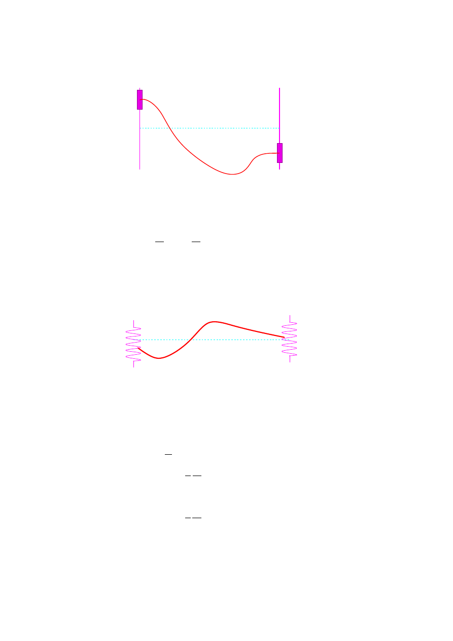
Consider a string with ends fastened to air bearings that are fixed to a rod orthogonal to the x-axis. Since the
bearings float freely there should be no force along the rods, which means that the string is horizontal at the
bearings, see Fig. 3.3 for a sketch.
18
CHAPTER 3. BOUNDARY AND INITIAL CONDITIONS
x=a
x=0
Figure 3.3: A string with floating endpoints.
It satisfies the wave equation with the same initial conditions as above, but the boundary conditions now
are
∂u
∂x
(0, t) =
∂u
∂x
(a, t) = 0,
t > 0.
(3.17)
These are clearly of von Neumann type.
3.3.3
A string with endpoints fixed to strings
To illustrate mixed boundary conditions we make an even more complicated contraption where we fix the
endpoints of the string to springs, with equilibrium at y = 0, see Fig. 3.4 for a sketch.
x=0
x=a
Figure 3.4: A string with endpoints fixed to springs.
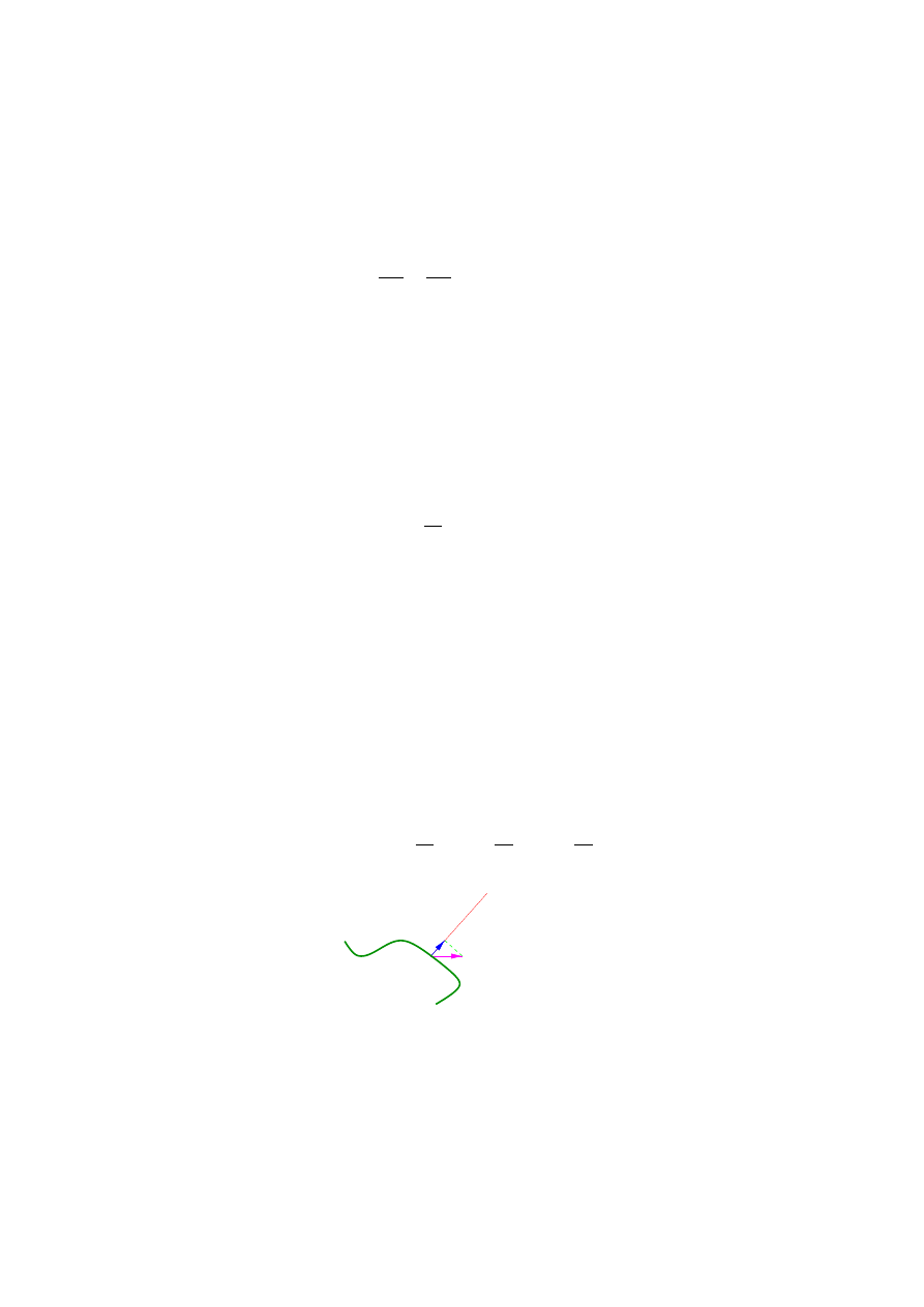
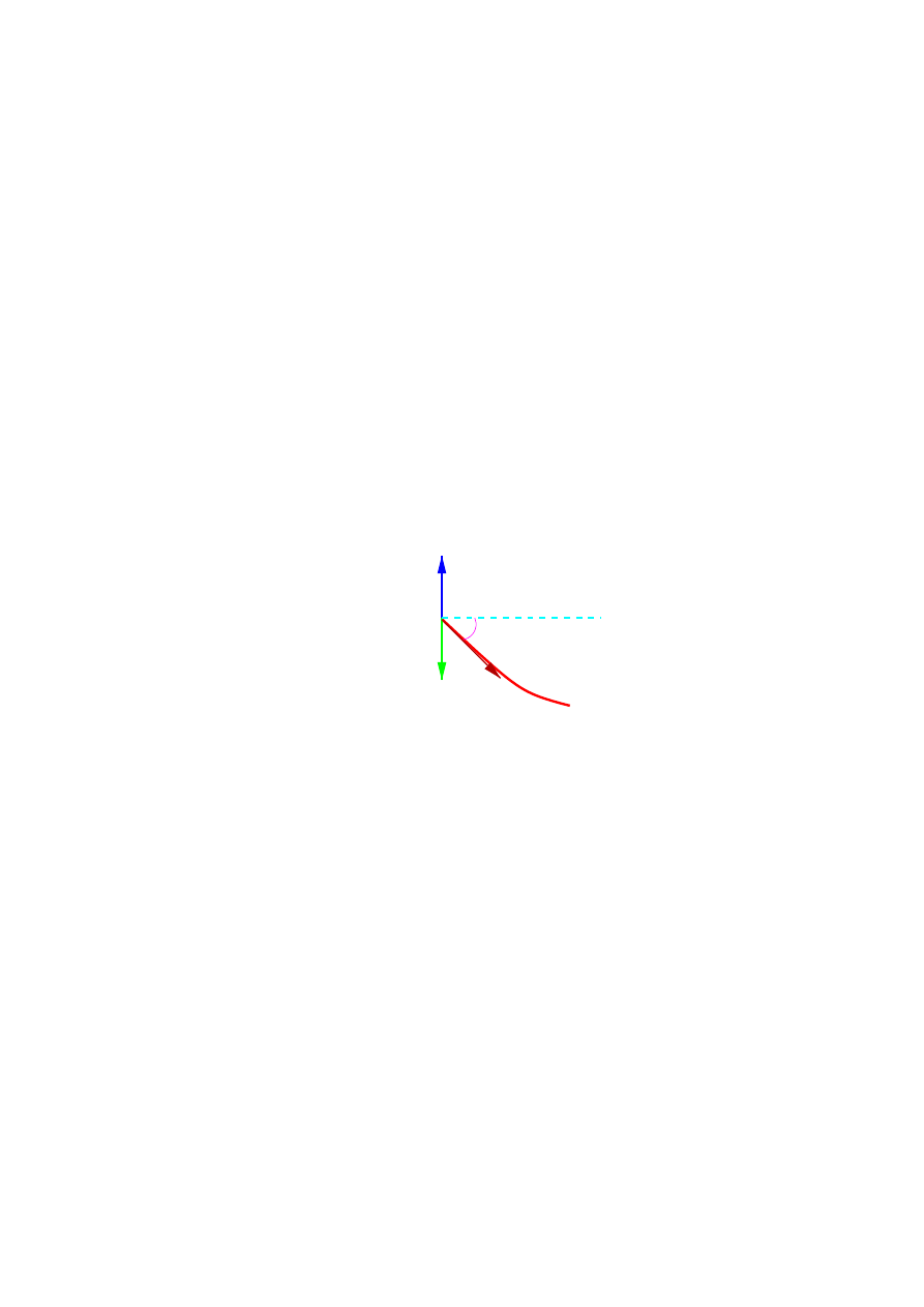
Hook’s law states that the force exerted by the spring (along the y axis) is F = −ku(0, t), where k is the
spring constant. This must be balanced by the force the string on the spring, which is equal to the tension
T in the string. The component parallel to the y axis is T sin α, where α is the angle with the horizontal, see
Fig. 3.5.
For small α we have sin α ≈ tan α =
∂u
∂x
(0, t). Since both forces should cancel we find
u(0, t) −
T
k
∂u
∂x
(0, t) = 0,
t > 0,
(3.18)
and
u(a, t) −
T
k
∂u
∂x
(a, t) = 0,
t > 0.
(3.19)
These are mixed boundary conditions.
3.3. A SLIGHTLY MORE REALISTIC EXAMPLE
19
parallel
to beam
force from
spring
α
String tension
Figure 3.5: the balance of forces at one endpoint of the string of Fig. 3.4.

20
CHAPTER 3. BOUNDARY AND INITIAL CONDITIONS

Chapter 4
Fourier Series
In this chapter we shall discuss Fourier series. These infinite series occur in many different areas of physics,
in electromagnetic theory, electronics, wave phenomena and many others. They have some similarity to – but
are very different from – the Taylor’s series you have encountered before.
4.1
Taylor series
One series you have encountered before is Taylor’s series,
f (x) =
∞
X
n=0
f
(n)
(a)
(x − a)
n
n!
,
(4.1)
where f
(n)
(x) is the nth derivative of f . An example is the Taylor series of the cosine around x = 0 (i.e.,
a = 0),
cos(0)
= 1,
cos
0
(x) = − sin(x),
cos
0
(0)
= 0,
cos
(2)
(x) = − cos(x),
cos
(2)
(0)=
−1,
(4.2)
cos
(3)
(x) = sin(x),
cos
(3)
(0) = 0,
cos
(4)
(x) = cos(x),
cos
(4)
(0) = 1.
Notice that after four steps we are back where we started. We have thus found (using m = 2n in (4.1)) )
cos x =
∞
X
m=0
(
−1)
m
(2m)!
x
2m
,
(4.3)
Question:
Show that
sin x =
∞
X
m=0
(−1)
m
(2m + 1)!
x
2m+1
.
(4.4)
4.2
Introduction to Fourier Series
Rather than Taylor series, that are supposed to work for “any” function, we shall study periodic functions.
For periodic functions the French mathematician introduced a series in terms of sines and cosines,
f (x) =
a
0
2
+
X
n=1
[a
n
cos(nx) + b
n
sin(nx)].
(4.5)
21

22
CHAPTER 4. FOURIER SERIES
We shall study how and when a function can be described by a Fourier series. One of the very important
differences with Taylor series is that they can be used to approximate non-continuous functions as well as
continuous ones.
4.3
Periodic functions
We first need to define a periodic function. A function is called periodic with period p if f (x + p) = f (x), for
all x, even if f is not defined everywhere. A simple example is the function f (x) = sin(bx) which is periodic
with period (2π)/b. Of course it is also periodic with periodic (4π)/b. In general a function with period p is
periodic with period 2p, 3p, . . .. This can easily be seen using the definition of periodicity, which subtracts p
from the argument
f (x + 3p) = f (x + 2p) = f (x + p) = f (x).
(4.6)
The smallest positive value of p for which f is periodic is called the (primitive) period of f .
Question:
What is the primitive period of sin(4x)?
Answer:
π/2.
4.4
Orthogonality and normalisation
Consider the series
a
0
2
+
X
n=1
[a
n
cos
nπx
L
+ b
n
sin
nπx
L
],
−L ≤ x ≤ L.
(4.7)
This is called a trigonometric series. If the series approximates a function f (as will be discussed) it is called
a Fourier series and a and b are the Fourier coefficients of f .
In order for all of this to make sense we first study the functions
{1, cos
nπx
L
, sin
nπx
L
},
n = 1, 2, . . .
,
(4.8)
and especially their properties under integration. We find that
Z
L
−L
1 · 1 dx = 2L,
(4.9)
Z
L
−L
1
· cos
nπx
L
dx
= 0,
(4.10)
Z
L
−L
1 · sin
nπx
L
dx
= 0,
(4.11)
Z
L
−L
cos
mπx
L
· cos
nπx
L
dx
=
1
2
Z
L
−L
cos
(m + n)πx
L
+ cos
(m − n)πx
L
dx
=
(
0
if n 6= m
L
if n = m
,
(4.12)
Z
L
−L
sin
mπx
L
· sin
nπx
L
dx
=
1
2
Z
L
−L
− cos
(m + n)πx
L
+ cos
(m − n)πx
L
dx
=
(
0
if n 6= m
L
if n = m
,
(4.13)
Z
L
−L
cos
mπx
L
· sin
nπx
L
dx
=
1
2
Z
L
−L
sin
(m + n)πx
L
+ sin
(m
− n)πx
L
dx
=
0.
(4.14)

4.5. WHEN IS IT A FOURIER SERIES?
23
If we consider these integrals as some kind of inner product between functions (like the standard vector inner
product) we see that we could call these functions orthogonal. This is indeed standard practice, where for
functions the general definition of inner product takes the form
(f, g) =
Z
b
a
w(x)f (x)g(x) dx.
(4.15)
If this is zero we say that the functions f and g are orthogonal on the interval [a, b] with weight function w. If
this function is 1, as is the case for the trigonometric functions, we just say that the functions are orthogonal
on [a, b].
The norm of a function is now defined as the square root of the inner-product of a function with itself
(again, as in the case of vectors),
||f|| =
sZ
b
a
w(x)f (x)
2
dx.
(4.16)
If we define a normalised form of f (like a unit vector) as f /||f||, we have
||(f/||f||)|| =
s R
b
a
w(x)f (x)
2
dx
||f||
2
=
qR
b
a
w(x)f (x)
2
dx
||f||
=
||f||
||f||
= 1.
(4.17)
Question:
What is the normalised form of {1, cos
nπx
L
, sin
nπx
L
}?
Answer:
{1/
√
2L, (1/
√
L) cos
nπx
L
, (1/
√
L) sin
nπx
L
}.
A set of mutually orthogonal functions that are all normalised is called an orthonormal set.
4.5
When is it a Fourier series?
The series discussed before are only useful is we can associate a function with them. How can we do that?
Lets us assume that the periodic function f (x) has a Fourier series representation (exchange the summation
and integration, and use orthogonality),
f (x) =
a
0
2
+
∞
X
n=1
h
a
n
cos
nπx
L
+ b
n
sin
nπx
L
i
.
(4.18)
We can now use the orthogonality of the trigonometric functions to find that
1
L
Z
L
−L
f (x) · 1dx = a
0
,
(4.19)
1
L
Z
L
−L
f (x) · cos
nπx
L
dx
=
a
n
,
(4.20)
1
L
Z
L
−L
f (x)
· sin
nπx
L
dx
=
b
n
.
(4.21)
This defines the Fourier coefficients for a given f (x). If these coefficients all exist we have defined a Fourier
series, about whose convergence we shall talk in a later lecture.
An important property of Fourier series is given in Parseval’s lemma:
Z
L
−L
f (x)
2
dx =
La
2
0
2
+ L
∞
X
n=1
(a
2
n
+ b
2
n
).
(4.22)
This looks like a triviality, until one realises what we have done: we have once again interchanged an infinite
summation and an integration. There are many cases where such an interchange fails, and actually it make a
24
CHAPTER 4. FOURIER SERIES
strong statement about the orthogonal set when it holds. This property is usually referred to as completeness.
We shall only discuss complete sets in these lectures.
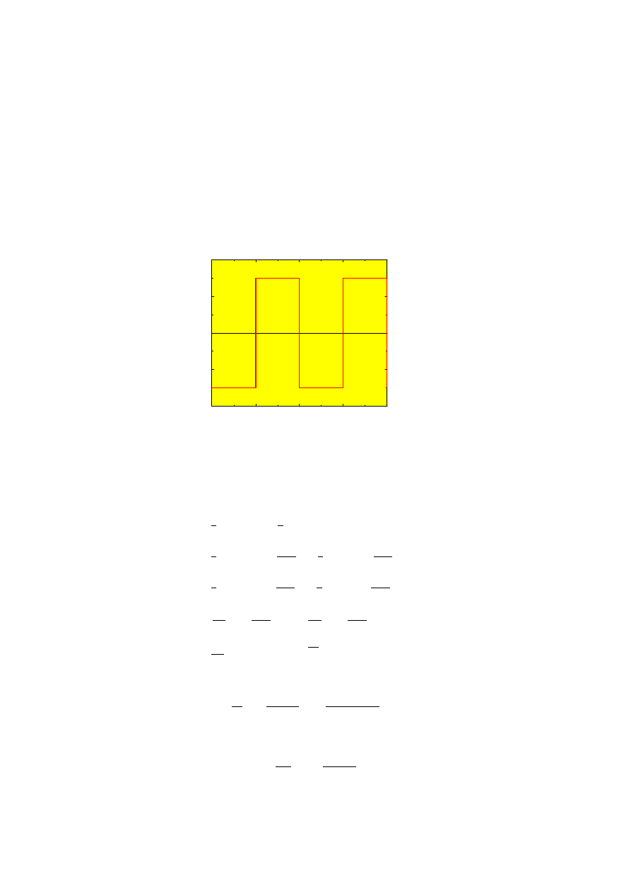
Now let us study an example. We consider a square wave (this example will return a few times)
f (x) =
(
−3
if −5 + 10n < x < 10n
3
if 10n < x < 5 + 10n
,
(4.23)
where n is an integer, as sketched in Fig. 4.1.
−5
0
5
10
15
x
−4
−2
0
2
4
y
Figure 4.1: The square wave (4.23).
This function is not defined at x = 5n. We easily see that L = 5. The Fourier coefficients are
a
0
=
1
5
Z
0
−5
−3dx +
1
5
Z
5
0
3dx = 0
a
n
=
1
5
Z
0
−5
−3 cos
nπx
5
+
1
5
Z
5
0
3 cos
nπx
5
= 0
(4.24)
b
n
=
1
5
Z
0
−5
−3 sin
nπx
5
+
1
5
Z
5
0
3 sin
nπx
5
=
3
nπ
cos
nπx
5
0
−5
−
3
nπ
cos
nπx
5
5
0
=
6
nπ
[1 − cos(nπ)] =
(
12
nπ
if n odd
0
if n even
And thus (n = 2m + 1)
f (x) =
12
π
X
m=0
1
2m + 1
sin
(2m + 1)πx
5
.
(4.25)
Question:
What happens if we apply Parseval’s theorem to this series?
Answer:
We find
Z
5
−5
9dx = 5
144
π
2
∞
X
m=0
1
2m + 1
2
(4.26)

4.6. FOURIER SERIES FOR EVEN AND ODD FUNCTIONS
25
Which can be used to show that
∞
X
m=0
1
2m + 1
2
=
π
2
8
.
(4.27)
4.6
Fourier series for even and odd functions
Notice that in the Fourier series of the square wave (4.23) all coefficients a
n
vanish, the series only contains
sines. This is a very general phenomenon for so-called even and odd functions.
A function is called even if f (−x) = f(x), e.g. cos(x).
A function is called odd if f (−x) = −f(x), e.g. sin(x).
These have somewhat different properties than the even and odd numbers:
1. The sum of two even functions is even, and of two odd ones odd.
2. The product of two even or two odd functions is even.
3. The product of an even and an odd function is odd.
Question:
Which of the following functions is even or odd?
a) sin(2x), b) sin(x) cos(x), c) tan(x), d) x
2
, e) x
3
, f) |x|
Answer:
even: d, f; odd: a, b, c, e.
Now if we look at a Fourier series, the Fourier cosine series
f (x) =
a
0
2
+
∞
X
n=1
a
n
cos
nπ
L
x
(4.28)
describes an even function (why?), and the Fourier sine series
f (x) =
∞
X
n=1
b
n
sin
nπ
L
x
(4.29)
an odd function. These series are interesting by themselves, but play an especially important rˆole for functions
defined on half the Fourier interval, i.e., on [0, L] instead of [−L, L]. There are three possible ways to define a
Fourier series in this way, see Fig. 4.2
1. Continue f as an even function, so that f
0
(0) = 0.
2. Continue f as an odd function, so that f (0) = 0.
3. Neither of the two above. We now nothing about f at x = 0.
Of course these all lead to different Fourier series, that represent the same function on [0, L]. The usefulness
of even and odd Fourier series is related to the imposition of boundary conditions. A Fourier cosine series has
df /dx = 0 at x = 0, and the Fourier sine series has f (x = 0) = 0. Let me check the first of these statements:
d
dx
"
a
0
2
+
∞
X
n=1
a
n
cos
nπ
L
x
#
= −
π
L
∞
X
n=1
na
n
sin
nπ
L
x = 0
at x = 0.
(4.30)

26
CHAPTER 4. FOURIER SERIES
-L
L
-L
L
-L
L
Figure 4.2: A sketch of the possible ways to continue f beyond its definition region for 0 < x < L. From left
to right as even function, odd function or assuming no symmetry at all.
0
1
x
0
1
f(x)
Figure 4.3: The function y = 1 − x.
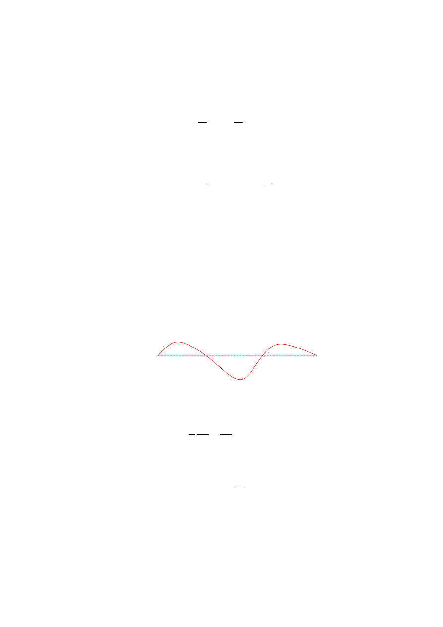
As an example look at the function f (x) = 1 − x, 0 ≤ x ≤ 1, with an even continuation on the interval
[
−1, 1]. We find
a
0
=
2
1
Z
1
0
(1
− x)dx = 1
a
n
= 2
Z
1
0
(1
− x) cos nπxdx
=
2
nπ
sin nπx −
2
n
2
π
2
[cos nπx + nπx sin nπx]
1
0
=
(
0
if n even
4
n
2
π
2
if n is odd
.
(4.31)
So, changing variables by defining n = 2m + 1 so that in a sum over all m n runs over all odd numbers,
f (x) =
1
2
+
4
π
2
∞
X
m=0
1
(2m + 1)
2
cos(2m + 1)πx.
(4.32)
4.7
Convergence of Fourier series
The final subject we shall consider is the convergence of Fourier series. I shall show two examples, closely
linked, but with radically different behaviour.
4.7. CONVERGENCE OF FOURIER SERIES
27
−
π
/2
π
/2
0
−
π
π
x
−
π
/2
π
/2
0
function
g(x)
f(x)
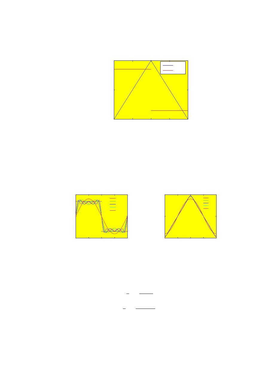
Figure 4.4: The square and triangular waves on their fundamental domain.
1. A square wave, f (x) = 1 for
−π < x < 0; f(x) = −1 for 0 < x < π.
2. a triangular wave, g(x) = π/2 + x for
−π < x < 0; g(x) = π/2 − x for 0 < x < π.
Note that f is the derivative of g.
−
π
/2
π
/2
0
−
π
π
x
−
π
/2
π
/2
0
f(x)
M=0
M=1
M=2
M=3
M=4
−
π
/2
π
/2
0
−
π
π
x
−
π
/2
π
/2
0
g(x)
M=0
M=1
M=2
M=3
M=4
Figure 4.5: The convergence of the Fourier series for the square (left) and triangular wave (right). the number
M is the order of the highest Fourier component.
It is not very hard to find the relevant Fourier series,
f (x) =
−
4
π
∞
X
m=0
1
2m + 1
sin(2m + 1)x,
(4.33)
g(x) =
4
π
∞
X
m=0
1
(2m + 1)
2
cos(2m + 1)x.
(4.34)
Let us compare the partial sums, where we let the sum in the Fourier series run from m = 0 to m = M instead
of m = 0 . . .
∞. We note a marked difference between the two cases. The convergence of the Fourier series of
28
CHAPTER 4. FOURIER SERIES
g is uneventful, and after a few steps it is hard to see a difference between the partial sums, as well as between
the partial sums and g. For f , the square wave, we see a surprising result: Even though the approximation
gets better and better in the (flat) middle, there is a finite (and constant!) overshoot near the jump. The
area of this overshoot becomes smaller and smaller as we increase M . This is called the Gibbs phenomenon
(after its discoverer). It can be shown that for any function with a discontinuity such an effect is present, and
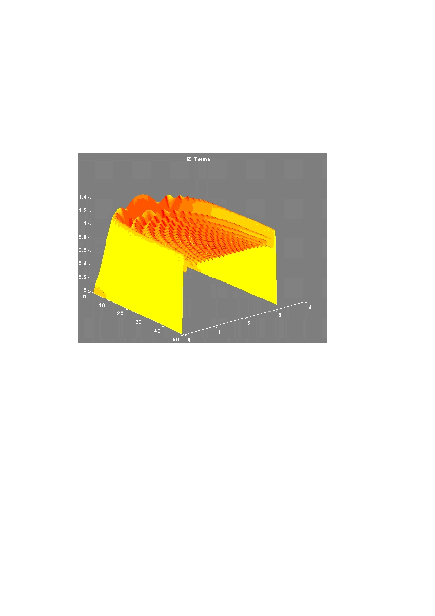
that the size of the overshoot only depends on the size of the discontinuity! A final, slightly more interesting
version of this picture, is shown in Fig. 4.6.
Figure 4.6: A three-dimensional representation of the Gibbs phenomenon for the square wave. The axis
orthogonal to the paper labels the number of Fourier components.

Chapter 5
Separation of variables on rectangular
domains
In this section we shall investigate two dimensional equations defined on rectangular domains. We shall either
look at finite rectangles, when we have two space variables, or at semi-infinite rectangles when one of the
variables is time. We shall study all three different types of equation.
5.1
Cookbook
Let me start with a recipe that describes the approach to separation of variables, as exemplified in the following
sections, and in later chapters. Try to trace the steps for all the examples you encounter in this course.
• Take care that the boundaries are naturally described in your variables (i.e., at the boundary one of the
coordinates is constant)!
• Write the unknown function as a product of functions in each variable.
• Divide by the function, so as to have a ratio of functions in one variable equal to a ratio of functions in
the other variable.
• Since these two are equal they must both equal to a constant.
• Separate the boundary and initial conditions. Those that are zero can be re-expressed as conditions on
one of the unknown functions.
• Solve the equation for that function where most boundary information is known.
• This usually determines a discrete set of separation parameters.
• Solve the remaining equation for each parameter.
• Use the superposition principle (true for homogeneous and linear equations) to add all these solutions
with an unknown constants multiplying each of the solutions.
• Determine the constants from the remaining boundary and initial conditions.
29

30
CHAPTER 5. SEPARATION OF VARIABLES ON RECTANGULAR DOMAINS
5.2
parabolic equation
Let us first study the heat equation in 1 space (and, of course, 1 time) dimension. This is the standard example
of a parabolic equation.
∂u
∂t
= k
∂
2
u
∂x
2
, 0 < x < L, t > 0.
(5.1)
with boundary conditions
u(0, t) = 0, u(L, t) = 0, t > 0,
(5.2)
and initial condition
u(x, 0) = x, 0 < x < L.
(5.3)
We shall attack this problem by separation of variables, a technique always worth trying when attempting to
solve a PDE,
u(x, t) = X(x)T (t).
(5.4)
This leads to the differential equation
X(x)T
0
(t) = kX”(x)T (t).
(5.5)
We find, by dividing both sides by XT , that
1
k
T
0
(t)
T (t)
=
X”(k)
X(k)
.
(5.6)
Thus the left-hand side, a function of t, equals a function of x on the right-hand side. This is not possible
unless both sides are independent of x and t, i.e. constant. Let us call this constant −λ.
We obtain two differential equations
T
0
(t) =
−λkT (t)
(5.7)
X”(x) =
−λX(x)
(5.8)
Question:
What happens if X(x)T (t) is zero at some point (x = x
0
, t = t
0
)?
Answer:
Nothing. We can still perform the same trick.
This is not so trivial as I suggest. We either have X(x
0
) = 0 or T (t
0
) = 0. Let me just
consider the first case, and assume T (t
0
) 6= 0. In that case we find (from (5.5)), substituting
t = t
0
, that X
00
(x
0
) = 0.
We now have to distinguish the three cases λ > 0, λ = 0, and λ < 0.
λ > 0
Write α
2
= λ, so that the equation for X becomes
X
00
(x) =
−α
2
X(x).
(5.9)
This has as solution
X(x) = A cos αx + B sin αx.
(5.10)
X(0) = 0 gives A · 1 + B · 0 = 0, or A = 0. Using X(L) = 0 we find that
B sin αL = 0
(5.11)
which has a nontrivial (i.e., one that is not zero) solution when αL = nπ, with n a positive integer. This leads
to λ
n
=
n
2
π
2
L
2
.

5.3. HYPERBOLIC EQUATION
31
λ = 0
We find that X = A + Bx. The boundary conditions give A = B = 0, so there is only the trivial (zero)
solution.
λ < 0
We write λ = −α
2
, so that the equation for X becomes
X
00
(x) =
−α
2
X(x).
(5.12)
The solution is now in terms of exponential, or hyperbolic functions,
X(x) = A cosh x + B sinh x.
(5.13)
The boundary condition at x = 0 gives A = 0, and the one at x = L gives B = 0. Again there is only a trivial
solution.
We have thus only found a solution for a discrete set of “eigenvalues” λ
n
> 0. Solving the equation for T
we find an exponential solution, T = exp(−λkT ). Combining all this information together, we have
u
n
(x, t) = exp
−k
n
2
π
2
L
2
t
sin
nπ
L
x
.
(5.14)
The equation we started from was linear and homogeneous, so we can superimpose the solutions for different
values of n,
u(x, t) =
∞
X
n=1
c
n
exp
−k
n
2
π
2
L
2
t
sin
nπ
L
x
.
(5.15)
This is a Fourier sine series with time-dependent Fourier coefficients. The initial condition specifies the
coefficients c
n
, which are the Fourier coefficients at time t = 0. Thus
c
n
=
2
L
Z
L
0
x sin
nπx
L
dx
= −
2L
nπ
(
−1)
n
= (−1)
n+1
2L
nπ
.
(5.16)
The final solution to the PDE + BC’s + IC is
u(x, t) =
∞
X
n=1
(
−1)
n+1
2L
nπ
exp
−k
n
2
π
2
L
2
t
sin
nπ
L
x.
(5.17)
This solution is transient: if time goes to infinity, it goes to zero.
5.3
hyperbolic equation
As an example of a hyperbolic equation we study the wave equation. One of the systems it can describe is a
transmission line for high frequency signals, 40m long.
∂
2
V
∂x
2
=
LC
|{z}
imp×capac
∂
2
V
∂t
2
∂V
∂x
(0, t) =
∂V
∂x
(40, t) = 0,
V (x, 0)
=
f (x),
∂V
∂t
(x, 0) = 0,
(5.18)

32
CHAPTER 5. SEPARATION OF VARIABLES ON RECTANGULAR DOMAINS
Separate variables,
V (x, t) = X(x)T (t).
(5.19)
We find
X
00
X
= LC
T
00
T
= −λ.
(5.20)
Which in turn shows that
X
00
=
−λX,
T
00
=
−
λ
LC
T.
(5.21)
We can also separate most of the initial and boundary conditions; we find
X
0
(0) = X
0
(40) = 0, T
0
(0) = 0.
(5.22)
Once again distinguish the three cases λ > 0, λ = 0, and λ < 0:
λ > 0 (almost identical to previous problem) λ
n
= α
2
n
, α
n
=
nπ
40
, X
n
= cos(α
n
x). We find that
T
n
(t) = D
n
cos
nπt
40
√
LC
+ E
n
sin
nπt
40
√
LC
.
(5.23)
T
0
(0) = 0 implies E
n
= 0, and taking both together we find (for n ≥ 1)
V
n
(x, t) = cos
nπt
40
√
LC
cos
nπx
40
.
(5.24)
λ = 0 X(x) = A + Bx. B = 0 due to the boundary conditions. We find that T (t) = Dt + E, and D is 0 due to
initial condition. We conclude that
V
0
(x, t) = 1.
(5.25)
λ < 0 No solution.
Taking everything together we find that
V (x, t) =
a
0
2
+
∞
X
n=1
a
n
cos
nπt
40
√
LC
cos
nπx
40
.
(5.26)
The one remaining initial condition gives
V (x, 0) = f (x) =
a
0
2
+
∞
X
n=1
a
n
cos
nπx
40
.
(5.27)
Use the Fourier cosine series (even continuation of f ) to find
a
0
=
1
20
Z
40
0
f (x)dx,
a
n
=
1
20
Z
40
0
f (x) cos
nπx
40
dx.
(5.28)
5.4. LAPLACE’S EQUATION
33
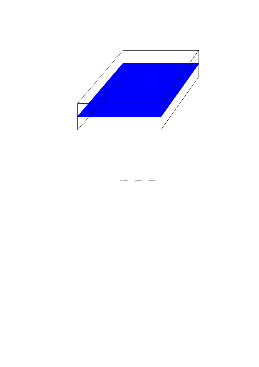
Figure 5.1: A conducting sheet insulated from above and below.
5.4
Laplace’s equation
In a square, heat-conducting sheet, insulated from above and below
1
k
∂u
∂t
=
∂
2
u
∂x
2
+
∂
2
u
∂y
2
.
(5.29)
If we are looking for a steady state solution, i.e. we take u(x, y, t) = u(x, y) the time derivative does not
contribute, and we get Laplace’s equation
∂
2
u
∂x
2
+
∂
2
u
∂y
2
= 0,
(5.30)
an example of an elliptic equation. Let us once again look at a square plate of size a
× b, and impose the
boundary conditions
u(x, 0) = 0,
u(a, y) = 0,
u(x, b) = x,
u(0, y)
= 0.
(5.31)
(This choice is made so as to be able to evaluate Fourier series easily. It is not very realistic!) We once again
separate variables,
u(x, y) = X(x)Y (y),
(5.32)
and define
X
00
X
= −
Y
00
Y
= −λ.
(5.33)
Or explicitly
X
00
= −λX, Y
00
= λY.
(5.34)
With boundary conditions X(0) = X(a) = 0, Y (0) = 0. The 3rd boundary conditions remains to be imple-
mented.
34
CHAPTER 5. SEPARATION OF VARIABLES ON RECTANGULAR DOMAINS
Once again distinguish three cases:
λ > 0 X(x) = sin α
n
(x), α
n
=
nπ
a
, λ
n
= α
2
n
. We find
Y (y)
=
C
n
sinh α
n
y + D
n
cosh α
n
y
= C
0
n
exp(α
n
y) + D
0
n
exp(−α
n
y).
(5.35)
Since Y (0) = 0 we find D
n
= 0 (sinh(0) = 0, cosh(0) = 1).
λ ≤ 0 No solutions
So we have
u(x, y) =
∞
X
n=1
b
n
sin α
n
x sinh α
n
y
(5.36)
The one remaining boundary condition gives
u(x, b) = x =
∞
X
n=1
b
n
sin α
n
x sinh α
n
b.
(5.37)
This leads to the Fourier series of x,
b
n
sinh α
n
b
=
2
a
Z
a
0
x sin
nπx
a
dx
=
2a
nπ
(−1)
n+1
.
(5.38)
So, in short, we have
V (x, y) =
2a
π
∞
X
n=1
(−1)
n+1
sin
nπx
a
sinh
nπy
a
n sinh
nπb
a
.
(5.39)
Question:
The dependence on x enters through a trigonometric function, and that on y through a hyperbolic
function. Yet the differential equation is symmetric under interchange of x and y. What happens?
Answer:
The symmetry is broken by the boundary conditions.
5.5
More complex initial/boundary conditions
It is not always possible on separation of variables to separate initial or boundary conditions in a condition on
one of the two functions. We can either map the problem into simpler ones by using superposition of boundary
conditions, a way discussed below, or we can carry around additional integration constants.
x=a
x=0
Let me give an example of these procedures. Consider a vibrating string attached to two air bearings,
gliding along rods 4m apart. You are asked to find the displacement for all times, if the initial displacement,
i.e. at t = 0s is one meter and the initial velocity is x/t
0
m/s.

5.5. MORE COMPLEX INITIAL/BOUNDARY CONDITIONS
35
The differential equation and its boundary conditions are easily written down,
∂
2
u
∂x
2
=
1
c
2
∂
2
u
∂t
2
,
∂u
∂x
(0, t) =
∂u
∂x
(4, t) = 0, t > 0,
u(x, 0) = 1,
∂u
∂t
(x, 0) =
x/t
0
.
(5.40)
Question:
What happens if I add two solutions v and w of the differential equation that satisfy the same
BC’s as above but different IC’s,
v(x, 0) = 0
,
∂v
∂t
(x, 0) = x/t
0
,
w(x, 0) = 1
,
∂w
∂t
(x, 0) = 0?
(5.41)
Answer:
u=v + w, we can add the BC’s.
If we separate variables, u(x, t) = X(x)T (t), we find that we obtain easy boundary conditions for X(x),
X
0
(0) = X
0
(4) = 0,
(5.42)
but we have no such luck for (t). As before we solve the eigenvalue equation for X, and find solutions for
λ
n
=
n
2
π
2
16
, n = 0, 1, ..., and X
n
= cos(
nπ
4
x). Since we have no boundary conditions for T (t), we have to take
the full solution,
T
0
(t) =
A
0
+ B
0
t,
T
n
(t) =
A
n
cos
nπ
4
ct + B
n
sin
nπ
4
ct,
(5.43)
and thus
u(x, t) =
1
2
(A
0
+ B
0
t) +
∞
X
n=1
A
n
cos
nπ
4
ct + B
n
sin
nπ
4
ct
cos
nπ
4
x.
(5.44)
Now impose the initial conditions
a)
u(x, 0) = 1 =
1
2
A
0
+
∞
X
n=1
A
n
cos
nπ
4
x,
(5.45)
which implies A
0
= 2, A
n
= 0, n > 0.
b)
∂u
∂t
(x, 0) = x/t
0
=
1
2
B
0
+
∞
X
n=1
nπc
4
B
n
cos
nπ
4
x.
(5.46)
This is the Fourier sine-series of x, which we have encountered before, and leads to the coefficients B
0
= 4
and B
n
= −
64
n
3
π
3
c
if n is odd and zero otherwise.
So finally
u(x, t) = (1 + 2t) −
64
π
3
X
n odd
1
n
3
sin
nπct
4
cos
nπx
4
.
(5.47)

36
CHAPTER 5. SEPARATION OF VARIABLES ON RECTANGULAR DOMAINS
5.6
Inhomogeneous equations
Consider a rod of length 2m, laterally insulated (heat only flows inside the rod). Initially the temperature u is
1
k
sin
πx
2
+ 500 K.
(5.48)
The left and right ends are both attached to a thermostat, and the temperature at the left side is fixed at
a temperature of 500 K and the right end at 100 K. There is also a heater attached to the rod that adds a
constant heat of sin
πx
2
to the rod. The differential equation describing this is inhomogeneous
∂u
∂t
= k
∂
2
u
∂x
2
+ sin
πx
2
,
u(0, t) =
500,
u(2, t) = 100,
u(x, 0)
=
1
k
sin
πx
2
+ 500.
(5.49)
Since the inhomogeneity is time-independent we write
u(x, t) = v(x, t) + h(x),
(5.50)
where h will be determined so as to make v satisfy a homogeneous equation. Substituting this form, we find
∂v
∂t
= k
∂
2
v
∂x
2
+ kh
00
+ sin
πx
2
.
(5.51)
To make the equation for v homogeneous we require
h
00
(x) = −
1
k
sin
πx
2
,
(5.52)
which has the solution
h(x) = C
1
x + C
2
+
4
kπ
2
sin
πx
2
.
(5.53)
At the same time we let h carry the boundary conditions, h(0) = 500, h(2) = 100, and thus
h(x) =
−200x + 500 +
4
kπ
2
sin
πx
2
.
(5.54)
The function v satisfies
∂v
∂t
=
k
∂
2
v
∂x
2
,
v(0, t) = v(π, t) = 0,
v(x, 0) = u(x, 0) − h(x) = 200x.
(5.55)
This is a problem of a type that we have seen before. By separation of variables we find
v(x, t) =
∞
X
n=1
b
n
exp(−
n
2
π
2
4
kt) sin
nπ
2
x.
(5.56)
The initial condition gives
∞
X
n=1
b
n
sin nx = 200x.
(5.57)
5.6. INHOMOGENEOUS EQUATIONS
37
from which we find
b
n
= (−1)
n+1
800
nπ
.
(5.58)
And thus
u(x, t) = −
200
x
+ 500 +
4
π
2
k
sin
πx
2
+
800
π
∞
X
n=1
(−1)
n
n + 1
sin
πnx
2
e
−k(nπ/2)
2
t
.
(5.59)
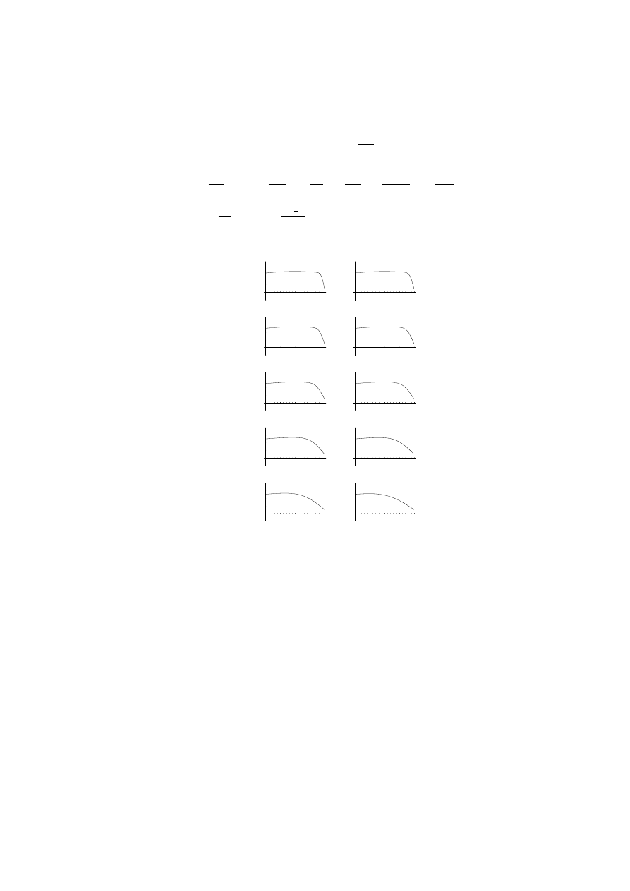
Note: as t
→ ∞, u(x, t) → −
400
π
x + 500 +
sin
π
2
x
k
. As can be seen in Fig. 5.2 this approach is quite rapid – we
have chosen k = 1/500 in that figure, and summed over the first 60 solutions.
0.5
1
1.5
2
x
-
200
200
400
600
800
u
t
=
15.8489
0.5
1
1.5
2
x
-
200
200
400
600
800
u
t
=
25.1189
0.5
1
1.5
2
x
-
200
200
400
600
800
u
t
=
6.30957
0.5
1
1.5
2
x
-
200
200
400
600
800
u
t
=
10.
0.5
1
1.5
2
x
-
200
200
400
600
800
u
t
=
2.51189
0.5
1
1.5
2
x
-
200
200
400
600
800
u
t
=
3.98107
0.5
1
1.5
2
x
-
200
200
400
600
800
u
t
=
1.
0.5
1
1.5
2
x
-
200
200
400
600
800
u
t
=
1.58489
0.5
1
1.5
2
x
-
200
200
400
600
800
u
t
=
0.398107
0.5
1
1.5
2
x
-
200
200
400
600
800
u
t
=
0.630957
Figure 5.2: Time dependence of the solution to the inhomogeneous equation (5.59)

38
CHAPTER 5. SEPARATION OF VARIABLES ON RECTANGULAR DOMAINS
Chapter 6
D’Alembert’s solution to the wave
equation
I have argued before that it is usually not useful to study the general solution of a partial differential equation.
As any such sweeping statement it needs to be qualified, since there are some exceptions. One of these is the
one-dimensional wave equation
∂
2
u
∂x
2
(x, t) −
1
c
2
∂
2
u
∂t
2
(x, t) = 0,
(6.1)
which has a general solution, due to the French mathematician d’Alembert.
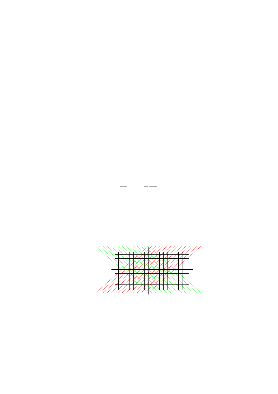
The reason for this solution becomes obvious when we consider the physics of the problem: The wave
equation describes waves that propagate with the speed c (the speed of sound, or light, or whatever). Thus
any perturbation to the one dimensional medium will propagate either right- or leftwards with such a speed.
This means that we would expect the solutions to propagate along the characteristics x ± ct = constant, as
seen in Fig. 6.1.
y
x
Figure 6.1: The change of variables from x and t to w = x + ct and z = x − ct.
In order to understand the solution in all mathematical details we make a change of variables
w = x + ct,
z = x − ct.
(6.2)
39

40
CHAPTER 6. D’ALEMBERT’S SOLUTION TO THE WAVE EQUATION
We write u(x, t) = ¯
u(w, z). We find
∂u
∂x
=
∂ ¯
u
∂w
∂w
∂x
+
∂ ¯
u
∂z
∂z
∂x
=
∂ ¯
u
∂w
+
∂ ¯
u
∂z
,
∂
2
u
∂x
2
=
∂
2
¯
u
∂w
2
+ 2
∂
2
¯
u
∂w∂z
+
∂ ¯
u
∂z
,
∂u
∂t
=
∂ ¯
u
∂w
∂w
∂t
+
∂ ¯
u
∂z
∂z
∂t
= c
∂ ¯
u
∂w
−
∂ ¯
u
∂z
,
∂
2
u
∂t
2
=
c
2
∂
2
¯
u
∂w
2
− 2
∂
2
¯
u
∂w∂z
+
∂ ¯
u
∂z
(6.3)
We thus conclude that
∂
2
u
∂x
2
(x, t) −
1
c
2
∂
2
u
∂t
2
(x, t) = 4
∂
2
¯
u
∂w∂z
= 0
(6.4)
An equation of the type
∂
2
¯
u
∂w∂z
= 0 can easily be solved by subsequent integration with respect to z and w.
First solve for the z dependence,
∂ ¯
u
∂w
= Φ(w),
(6.5)
where Φ is any function of w only. Now solve this equation for the w dependence,
¯
u(w, z) =
Z
Φ(w)dw = F (w) + G(z)
(6.6)
In other words,
u(x, t) = F (x + ct) + G(x
− ct) ,
(6.7)
with F and G arbitrary functions.
This equation is quite useful in practical applications. Let us first look at how to use this when we have
an infinite system (no limits on x). Assume that we are treating a problem with initial conditions
u(x, 0) = f (x),
∂u
∂t
(x, 0) = g(x).
(6.8)
Let me assume f (±∞) = 0. I shall assume this also holds for F and G (we don’t have to, but this removes
some arbitrary constants that don’t play a rˆole in u). We find
F (x) + G(x) =
f (x),
c(F
0
(x) − G
0
(x)) =
g(x).
(6.9)
The last equation can be massaged a bit to give
F (x) − G(x) =
1
c
Z
x
0
g(y)dy
|
{z
}
=Γ(x)
+C
(6.10)
Note that Γ is the integral over g. So Gamma will always be a continuous function, even if g is not!
And in the end we have
F (x) =
1
2
[f (x) + Γ(x) + C]
G(x) =
1
2
[f (x) − Γ(x) − C]
(6.11)
Suppose we choose (for simplicity we take c = 1m/s)
f (x) =
x + 1
if −1 < x < 0
1 − x if 0 < x < 1
0
elsewhere
.
(6.12)
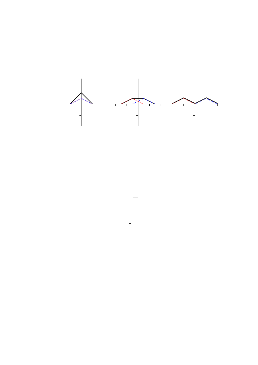
41
and g(x) = 0. The solution is then simply given by
u(x, t) =
1
2
[f (x + t) + f (x
− t)] .
(6.13)
This can easily be solved graphically, as shown in Fig. 6.2.
2
-2
-1
1
2
-2
-1
1
-2
-1
1
2
-1
1
1
-1
-1
1
Figure 6.2: The graphical form of (6.13), for (from left to right) t = 0s,t = 0.5s and t = 1s. The dashed lines
are
1
2
f (x + t) (leftward moving wave) and
1
2
f (x − t) (rightward moving wave). The solid line is the sum of
these two, and thus the solution u.
.
The case of a finite string is more complex. There we encounter the problem that even though f and g
are only known for 0 < x < a, x ± ct can take any value from −∞ to ∞. So we have to figure out a way to
continue the function beyond the length of the string. The way to do that depends on the kind of boundary
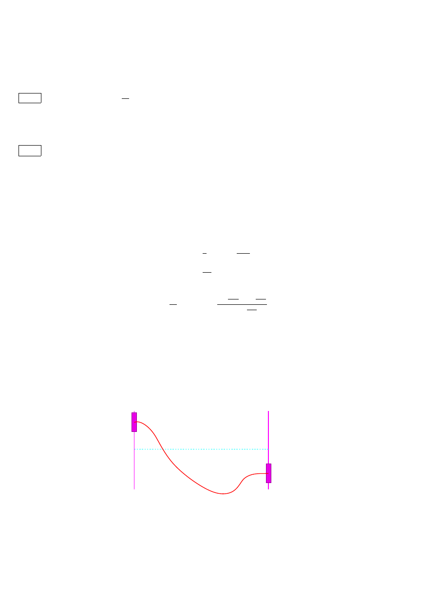
conditions: Here we shall only consider a string fixed at its ends.
u(0, t) = u(a, t) = 0,
u(x, 0) = f (x)
∂u
∂t
(x, 0) = g(x).
(6.14)
Initially we can follow the approach for the infinite string as sketched above, and we find that
F (x)
=
1
2
[f (x) + Γ(x) + C] ,
G(x) =
1
2
[f (x) − Γ(x) − C] .
(6.15)
Look at the boundary condition u(0, t) = 0. It shows that
1
2
[f (ct) + f (
−ct)] +
1
2
[Γ(ct) − Γ(−ct)] = 0.
(6.16)
Now we understand that f and Γ are completely arbitrary functions – we can pick any form for the initial
conditions we want. Thus the relation found above can only hold when both terms are zero
f (x) =
−f(−x),
Γ(x) = Γ(x).
(6.17)
Now apply the other boundary condition, and find
f (a + x) =
−f(a − x),
Γ(a + x) =
Γ(a − x).
(6.18)
The reflection conditions for f and Γ are similar to those for sines and cosines, and as we can see see from
Fig. 6.3 both f and Γ have period 2a.
Now let me look at two examples

42
CHAPTER 6. D’ALEMBERT’S SOLUTION TO THE WAVE EQUATION
x=0
x=a
Figure 6.3: A schematic representation of the reflection conditions (6.17,6.18). The dashed line represents f
and the dotted line Γ.
Example 6.1:
Find graphically a solution to
∂
2
u
∂t
2
=
∂
2
u
∂x
2
(c = 1m/s)
u(x, 0)
=
(
2x
if 0
≤ x ≤ 2
24/5
− 2x/5 if 2 ≤ x ≤ 12
.
∂u
∂t
(x, 0) =
0
u(0, t) =
u(12, t) = 0
(6.19)
Solution:
We need to continue f as an odd function, and we can take Γ = 0. We then have to add the
left-moving wave
1
2
f (x + t) and the right-moving wave
1
2
f (x − t), as we have done in Figs. ???
Example 6.2:
Find graphically a solution to
∂
2
u
∂t
2
=
∂
2
u
∂x
2
(c = 1m/s)
u(x, 0) =
0
∂u
∂t
(x, 0) =
(
1 if 4 ≤ x ≤ 6
0 elsewhere
.
u(0, t) =
u(12, t) = 0.
(6.20)
Solution:

43
In this case f = 0. We find
Γ(x) =
Z
x
0
g(x
0
)dx
0
=
0
if 0 < x < 4
−4 + x if 4 < x < 6
2
if 6 < x < 12
.
(6.21)
This needs to be continued as an even function.

44
CHAPTER 6. D’ALEMBERT’S SOLUTION TO THE WAVE EQUATION
Chapter 7
Polar and spherical coordinate systems
7.1
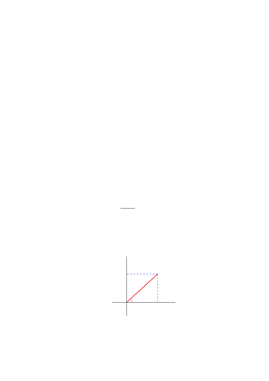
Polar coordinates
Polar coordinates in two dimensions are defined by
x = ρ cos φ, y = ρ sin φ,
(7.1)
ρ =
p
x
2
+ y
2
, φ = arctan(y/x),
(7.2)
as indicated schematically in Fig. 7.1.
x
y
ρ
ϕ
Figure 7.1: Polar coordinates
45

46
CHAPTER 7. POLAR AND SPHERICAL COORDINATE SYSTEMS
Using the chain rule we find
∂
∂x
=
∂ρ
∂x
∂
∂ρ
+
∂φ
∂x
∂
∂φ
=
x
ρ
∂
∂ρ
−
y
ρ
2
∂
∂φ
=
cos φ
∂
∂ρ
−
sin φ
ρ
∂
∂φ
,
(7.3)
∂
∂y
=
∂ρ
∂y
∂
∂ρ
+
∂φ
∂y
∂
∂φ
=
y
ρ
∂
∂ρ
+
x
ρ
2
∂
∂φ
=
sin φ
∂
∂ρ
+
cos φ
ρ
∂
∂φ
,
(7.4)
We can write
∇ = ˆe
ρ
∂
∂ρ
+ ˆ
e
φ
1
ρ
∂
∂φ
(7.5)
where the unit vectors
ˆ
e
ρ
= (cos φ, sin φ),
ˆ
e
φ
= (− sin φ, cos φ),
(7.6)
are an orthonormal set. We say that circular coordinates are orthogonal.
We can now use this to evaluate
∇
2
,
∇
2
= cos
2
φ
∂
2
∂ρ
2
+
sin φ cos φ
ρ
2
∂
∂φ
+
sin
2
φ
ρ
∂
∂ρ
+
sin
2
φ
ρ
2
∂
2
∂φ
2
+
sin φ cos φ
ρ
2
∂
∂φ
+ sin
2
φ
∂
2
∂ρ
2
−
sin φ cos φ
ρ
2
∂
∂φ
+
cos
2
φ
ρ
∂
∂ρ
+
cos
2
φ
ρ
2
∂
2
∂φ
2
−
sin φ cos φ
ρ
2
∂
∂φ
(7.7)
=
∂
2
∂ρ
2
+
1
ρ
∂
∂ρ
+
1
ρ
2
∂
2
∂φ
2
=
1
ρ
∂
∂ρ
ρ
∂
∂ρ
+
1
ρ
2
∂
2
∂φ
2
.
(7.8)
A final useful relation is the integration over these coordinates.
As indicated schematically in Fig. 7.2, the surface related to a change ρ → ρ + δρ, φ → φ + δφ is ρδρδφ.
This leads us to the conclusion that an integral over x, y can be rewritten as
Z
V
f (x, y)dxdy =
Z
V
f (ρ cos φ, ρ sin φ)ρdρdφ
(7.9)
7.2
spherical coordinates
Spherical coordinates are defined as
x = r cos φ sin θ, y = r sin φ sin θ, z = r cos θ,
(7.10)
r =
p
x
2
+ y
2
+ z
2
, φ = arctan(y/x), θ = arctan
p
x
2
+ y
2
z
!
,
(7.11)
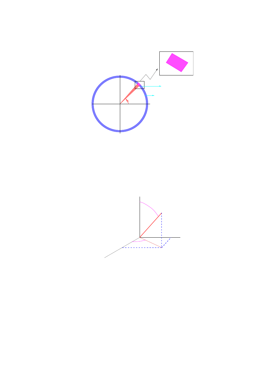
7.2. SPHERICAL COORDINATES
47
ϕ
ρ+δρ
ρ
δρ
ρδϕ
Figure 7.2: Integration in polar coordinates
x
y
z
θ
φ
r
Figure 7.3: Spherical coordinates
as indicated schematically in Fig. 7.3.

48
CHAPTER 7. POLAR AND SPHERICAL COORDINATE SYSTEMS
Using the chain rule we find
∂
∂x
=
∂r
∂x
∂
∂r
+
∂φ
∂x
∂
∂φ
+
∂θ
∂x
∂
∂θ
=
x
r
∂
∂r
−
y
x
2
+ y
2
∂
∂φ
+
xz
r
2
p
x
2
+ y
2
∂
∂θ
= sin θ cos φ
∂
∂r
−
sin φ
r sin θ
∂
∂φ
+
cos φ cos θ
r
∂
∂θ
,
(7.12)
∂
∂y
=
∂r
∂y
∂
∂r
+
∂φ
∂y
∂
∂φ
+
∂θ
∂y
∂
∂θ
=
y
r
∂
∂r
+
x
x
2
+ y
2
∂
∂φ
+
yz
r
2
p
x
2
+ y
2
∂
∂θ
= sin θ sin φ
∂
∂r
+
cos φ
r sin θ
∂
∂φ
+
sin φ cos θ
r
∂
∂θ
,
(7.13)
∂
∂z
=
∂r
∂z
∂
∂r
+
∂φ
∂z
∂
∂φ
+
∂θ
∂z
∂
∂θ
=
z
r
∂
∂r
−
p
x
2
+ y
2
r
2
∂
∂θ
= sin θ sin φ
∂
∂r
−
sin θ
r
∂
∂θ
.
(7.14)
(7.15)
once again we can write ∇ in terms of these coordinates.
∇ = ˆe
r
∂
∂r
+ ˆ
e
φ
1
r sin θ
∂
∂φ
+ ˆ
e
θ
1
r
∂
∂θ
(7.16)
where the unit vectors
ˆ
e
r
= (sin θ cos φ, sin θ sin φ, cos θ),
ˆ
e
φ
= (− sin φ, cos φ, 0),
ˆ
e
θ
= (cos φ cos θ, sin φ cos θ, − sin θ).
(7.17)
are an orthonormal set. We say that spherical coordinates are orthogonal.
We can use this to evaluate ∆ =
∇
2
,
∆ =
1
r
2
∂
∂r
r
2
∂
∂r
+
1
r
2
1
sin θ
∂
∂θ
sin θ
∂
∂θ
+
1
r
2
∂
2
∂φ
2
(7.18)
Finally, for integration over these variables we need to know the volume of the small cuboid contained
between r and r + δr, θ and θ + δθ and φ and φ + δφ. The length of the sides due to each of these changes is
δr, rδθ and r sin θδθ, respectively. We thus conclude that
Z
V
f (x, y, z)dxdydz =
Z
V
f (r, θ, φ)r
2
sin θdrdθdφ.
(7.19)

7.2. SPHERICAL COORDINATES
49
φ φ+δφ
θ δφ
r
δθ
r
θ+δθ
r r+ r
δ
r sin
δ
θ
Figure 7.4: Integration in spherical coordinates

50
CHAPTER 7. POLAR AND SPHERICAL COORDINATE SYSTEMS

Chapter 8
Separation of variables in polar
coordinates
Consider a circular plate of radius c m, insulated from above and below. The temperature on the circumference
is 100
◦
C on half the circle, and 0
◦
C on the other half.
T=0
T=100
c
Figure 8.1: The boundary conditions for the temperature on a circular plate.
The differential equation to solve is
ρ
2
∂
2
u
∂ρ
2
+ ρ
∂u
∂ρ
+
∂
2
u
∂φ
2
= 0,
(8.1)
with boundary conditions
u(c, φ) =
(
100 if 0 < φ < π
0
if π < φ < 2π
.
(8.2)
There is no real boundary in the φ direction, but we introduce one, since we choose to let φ run from 0 to 2π
only. So what kind of boundary conditions do we apply? We would like to see “seamless behaviour”, which
specifies the periodicity of the solution in φ,
u(ρ, φ + 2π) = u(ρ, φ),
(8.3)
∂u
∂φ
(ρ, φ + 2π)
=
∂u
∂φ
(ρ, φ).
(8.4)
If we choose to put the seem at φ =
−π we have the periodic boundary conditions
u(ρ, 2π)
=
u(ρ, 0),
(8.5)
∂u
∂φ
(ρ, 2π)
=
∂u
∂φ
(ρ, 0).
(8.6)
51

52
CHAPTER 8. SEPARATION OF VARIABLES IN POLAR COORDINATES
We separate variables, and take, as usual
u(ρ, φ) = R(ρ)Φ(φ).
(8.7)
This gives the usual differential equations
Φ
00
− λΦ = 0,
(8.8)
ρ
2
R
00
+ ρR
0
+ λR
=
0.
(8.9)
Our periodic boundary conditions gives a condition on Φ,
Φ(0) = Φ(2π), Φ
0
(0) = Φ
0
(2π).
(8.10)
The other boundary condition involves both R and Φ.
As usual we consider the cases λ > 0, λ < 0 and λ = 0 separately. Consider the Φ equation first, since this
has the most restrictive explicit boundary conditions (8.10).
λ = −α
2
< 0 We have to solve
Φ
00
= α
2
Φ,
(8.11)
which has as a solution
Φ(φ) = A cos αφ + B sin αφ.
(8.12)
Applying the boundary conditions, we get
A
=
A cos(2απ) + B sin(2απ),
(8.13)
Bα
=
−Aα sin(2απ) + Bα cos(2απ).
(8.14)
If we eliminate one of the coefficients from the equation, we get
A = A cos(2απ) − A sin(2απ)
2
/(1 − cos(2απ))
(8.15)
which leads to
sin(2απ)
2
=
−(1 − cos(2απ))
2
,
(8.16)
which in turn shows
2 cos(2απ) = 2,
(8.17)
and thus we only have a non-zero solution for α = n, an integer. We have found
λ
n
= n
2
, Φ
n
(φ) = A
n
cos nφ + B
n
sin nφ.
(8.18)
λ = 0 We have
Φ
00
= 0.
(8.19)
This implies that
Φ = Aφ + B.
(8.20)
The boundary conditions are satisfied for A = 0,
Φ
0
(φ) = B
n
.
(8.21)
λ > 0 The solution (hyperbolic sines and cosines) cannot satisfy the boundary conditions.

53
Now let me look at the solution of the R equation for each of the two cases (they can be treated as one),
ρ
2
R
00
(ρ) + ρR
0
(ρ) − n
2
R(ρ) = 0.
(8.22)
Let us attempt a power-series solution (this method will be discussed in great detail in a future lecture)
R(ρ) = ρ
α
.
(8.23)
We find the equation
ρ
α
[α(α − 1) + α
2
− n
2
] = ρ
α
[α
2
− n
2
] = 0
(8.24)
If n
6= 0 we thus have two independent solutions (as should be)
R
n
(ρ) = Cρ
−n
+ Dρ
n
(8.25)
The term with the negative power of ρ diverges as ρ goes to zero. This is not acceptable for a physical quantity
(like the temperature). We keep the regular solution,
R
n
(ρ) = ρ
n
.
(8.26)
For n = 0 we find only one solution, but it is not very hard to show (e.g., by substitution) that the general
solution is
R
0
(ρ) = C
0
+ D
0
ln(ρ).
(8.27)
We reject the logarithm since it diverges at ρ = 0.
In summary, we have
u(ρ, φ) =
A
0
2
+
∞
X
n=1
ρ
n
(A
n
cos nφ + B
n
sin nφ) .
(8.28)
The one remaining boundary condition can now be used to determine the coefficients A
n
and B
n
,
U (c, φ)
=
A
0
2
+
∞
X
n=1
c
n
(A
n
cos nφ + B
n
sin nφ)
=
(
100 if 0 < φ < π
0
if π < φ < 2π
.
(8.29)
We find
A
0
=
1
π
Z
π
0
100 dφ = 100,
c
n
A
n
=
1
π
Z
π
0
100 cos nφ dφ =
100
nπ
sin(nφ)|
π
0
= 0,
c
n
B
n
=
1
π
Z
π
0
100 sin nφ dφ =
−
100
nπ
cos(nφ)|
π
0
=
(
200/(nπ) if n is odd
0
if n is even
.
(8.30)
In summary
u(ρ, φ) = 50 +
200
π
X
n odd
ρ
c
n
sin nφ
n
.
(8.31)
We clearly see the dependence of u on the pure number r/c, rather than ρ. A three dimensional plot of the
temperature is given in Fig. 8.2.
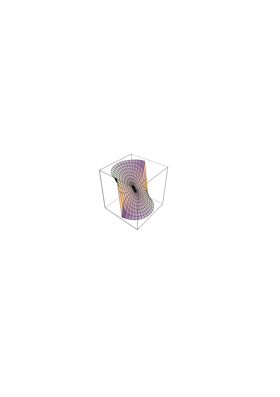
54
CHAPTER 8. SEPARATION OF VARIABLES IN POLAR COORDINATES
- 1
- 0.5
0
0.5
1
x
- 1
- 0.5
0
0.5
1
y
0
25
50
75
100
T
0
25
50
75
100
T
Figure 8.2: The temperature (8.31)

Chapter 9
Series solutions of O.D.E.
(Frobenius’ method)
Let us look at the a very simple (ordinary) differential equation,
y
00
(t) = t y(t),
(9.1)
with initial conditions y(0) = a, y
0
(0) = b. Let us assume that there is a solution that is analytical near t = 0.
This means that near t = 0 the function has a Taylor’s series
y(t) = c
0
+ c
1
t + . . . =
∞
X
k=0
c
k
t
k
.
(9.2)
(We shall ignore questions of convergence.) Let us proceed
y
0
(t) = c
1
+ 2c
2
t + . . . =
∞
X
k=1
kc
k
t
k−1
,
y
00
(t) =2c
2
+ 3 · 2t + . . . =
∞
X
k=2
k(k − 1)c
k
t
k
−2
,
ty(t) = c
0
t + c
1
t
2
+ . . . =
∞
X
k=0
c
k
t
k+1
.
(9.3)
Combining this together we have
y
00
− ty = [2c
2
+ 3 · 2t + . . .] − [c
0
t + c
1
t
2
+ . . .]
= 2c
2
+ (3 · 2c
3
− c
0
)t + . . .
= 2c
2
+
∞
X
k=3
{k(k − 1)c
k
− c
k
−3
} t
k−2
.
(9.4)
Here we have collected terms of equal power of t. The reason is simple. We are requiring a power series to
equal 0. The only way that can work is if each power of x in the power series has zero coefficient. (Compare
a finite polynomial....) We thus find
c
2
= 0, k(k − 1)c
k
= c
k−3
.
(9.5)
The last relation is called a recurrence of recursion relation, which we can use to bootstrap from a given value,
in this case c
0
and c
1
. Once we know these two numbers, we can determine c
3
,c
4
and c
5
:
c
3
=
1
6
c
0
, c
4
=
1
12
c
1
, c
5
=
1
20
c
2
= 0.
(9.6)
55

56
CHAPTER 9. SERIES SOLUTIONS OF O.D.E.
These in turn can be used to determine c
6
, c
7
, c
8
, etc. It is not too hard to find an explicit expression for the
c’s
c
3m
=
3m − 2
(3m)(3m − 1)(3m − 2)
c
3(m−1)
=
3m − 2
(3m)(3m − 1)(3m − 2)
3m
− 5
(3m − 3)(3m − 4)(3m − 5)
c
3(m−1)
=
(3m − 2)(3m − 5) . . . 1
(3m)!
c
0
,
c
3m+1
=
3m − 1
(3m + 1)(3m)(3m − 1)
c
3(m−1)+1
=
3m − 1
(3m + 1)(3m)(3m − 1)
3m − 4
(3m − 2)(3m − 3)(3m − 4)
c
3(m
−2)+1
=
(3m − 2)(3m − 5) . . . 2
(3m + 1)!
c
1
,
c
3m+1
= 0.
(9.7)
The general solution is thus
y(t) = a
"
1 +
∞
X
m=1
c
3m
t
3m
#
+ b
"
1 +
∞
X
m=1
c
3m+1
t
3m+1
#
.
(9.8)
The technique sketched here can be proven to work for any differential equation
y
00
(t) + p(t)y
0
(t) + q(t)y(t) = f (t)
(9.9)
provided that p(t), q(t) and f (t) are analytic at t = 0. Thus if p, q and f have a power series expansion, so
has y.
9.1
Singular points
As usual there is a snag. Most equations of interest are of a form where p and/or q are singular at the point t
0
(usually t
0
= 0). Any point t
0
where p(t) and q(t) are singular is called (surprise!) a singular point. Of most
interest are a special class of singular points called regular singular points, where the differential equation can
be given as
(t − t
0
)
2
y
00
(t) + (t − t
0
)α(t)y
0
(t) + β(t)y(t) = 0,
(9.10)
with α and β analytic at t = t
0
. Let us assume that this point is t
0
= 0. Frobenius’ method consists of the
following technique: In the equation
x
2
y
00
(x) + xα(x)y
0
(x) + β(x)y(x) = 0,
(9.11)
we assume a generalised series solution of the form
y(x) = x
γ
∞
X
n=0
c
n
x
k
.
(9.12)
Equating powers of x we find
γ(γ
− 1)c
0
x
γ
+ α
0
γc
0
x
γ
+ β
0
c
0
x
γ
= 0,
(9.13)
etc. The equation for the lowest power of x can be rewritten as
γ(γ
− 1) + α
0
γ + β
0
= 0.
(9.14)

9.2. *SPECIAL CASES
57
This is called the indicial equation . It is a quadratic equation in γ, that usually has two (complex) roots.
Let me call these γ
1
, γ
2
. If γ
1
− γ
2
is not integer one can prove that the two series solutions for y with these
two values of γ are independent solutions.
Let us look at an example
t
2
y
00
(t) +
3
2
ty
0
(t) + ty = 0.
(9.15)
Here α(t) = 3/2, β(t) = t, so t = 0 is indeed a regular singular point. The indicial equation is
γ(γ
− 1) +
3
2
γ = γ
2
+ γ/2 = 0.
(9.16)
which has roots γ
1
= 0, γ
2
= −1/2, which gives two independent solutions
y
1
(t) =
X
k
c
k
t
k
,
y
2
(t) =
t
−1/2
X
k
d
k
t
k
.
Independent solutions:
Independent solutions are really very similar to independent vectors: Two or more functions
are independent if none of them can be written as a combination of the others. Thus x
and 1 are independent, and 1 + x and 2 + x are dependent.
9.2
*Special cases
For the two special cases I will just give the solution. It requires a substantial amount of algebra to study
these two cases.
9.2.1
Two equal roots
If the indicial equation has two equal roots, γ
1
= γ
2
, we have one solution of the form
y
1
(t) = t
γ
1
∞
X
n=0
c
n
t
n
.
(9.17)
The other solution takes the form
y
2
(t) = y
1
(t) ln t + t
γ
1
+1
∞
X
n=0
d
n
t
n
.
(9.18)
Notice that this last solution is always singular at t = 0, whatever the value of γ
1
!
9.2.2
Two roots differing by an integer
If the indicial equation that differ by an integer, γ
1
− γ
2
= n > 0, we have one solution of the form
y
1
(t) = t
γ
1
∞
X
n=0
c
n
t
n
.
(9.19)
The other solution takes the form
y
2
(t) = ay
1
(t) ln t + t
γ
2
∞
X
n=0
d
n
t
n
.
(9.20)
The constant a is determined by substitution, and in a few relevant cases is even 0, so that the solutions can
be of the generalised series form.

58
CHAPTER 9. SERIES SOLUTIONS OF O.D.E.
9.2.3
Example 1
Find two independent solutions of
t
2
y
00
+ ty
0
+ ty = 0
(9.21)
near t = 0. The indicial equation is γ
2
= 0, so we get one solution of the series form
y
1
(t) =
X
n
c
n
t
n
.
(9.22)
We find
t
2
y
00
1
=
X
n
n(n
− 1)c
n
t
n
ty
0
1
=
X
n
nc
n
t
n
ty
1
=
X
n
c
n
t
n+1
=
X
n
0
c
n
0
−1
t
n
0
(9.23)
We add terms of equal power in x,
t
2
y
00
1
= 0 +
0t
+ 2c
2
t
2
+ 6c
3
t
3
+
. . .
ty
0
1
= 0 +
c
1
t
+ 2c
2
t
2
+ 3c
3
t
3
+
. . .
ty
1
= 0 +
c
0
t
+
c
1
t
2
+
c
2
t
3
+ . . .
t
2
y
00
+ ty
0
+ ty
= 0 + (c
1
+ c
0
)t + (4c
2
+ c
1
)t
2
+ (9c
3
+ c
2
)t
2
+
. . .
(9.24)
Both of these ways give
t
2
y
00
+ ty
0
+ ty =
∞
X
n=1
(c
n
n
2
+ c
n−1
)t
n
,
(9.25)
and lead to the recurrence relation
c
n
= −
1
n
2
c
n−1
(9.26)
which has the solution
c
n
= (−1)
n
1
n!
2
(9.27)
and thus
y
1
(t) =
∞
X
n=0
(−1)
n
1
n!
2
x
n
(9.28)
Let us look at the second solution
y
2
(t) = ln(t)y
1
(t) + t
∞
X
n=0
d
n
t
n
|
{z
}
y
3
(t)
(9.29)
Her I replace the power series with a symbol, y
3
for convenience. We find
y
0
2
= ln(t)y
0
1
+
y
1
(t)
t
+ y
0
3
y
00
2
= ln(t)y
00
1
+
2y
0
1
(t)
t
−
y
1
(t)
t
2
+ +y
00
3
(9.30)
Taking all this together, we have,
t
2
y
00
2
+ ty
0
2
+ ty
2
=
ln(t)(t
2
y
00
1
+ ty
0
1
+ ty
1
) − y
1
+ 2ty
0
1
+ y
1
+ t
2
y
00
3
+ ty
0
3
+ y
3
=
2ty
0
1
+ t
2
y
00
3
+ ty
0
3
+ ty
3
) = 0.
(9.31)

9.2. *SPECIAL CASES
59
If we now substitute the series expansions for y
1
and y
3
we get
2c
n
+ d
n
(n + 1)
2
+ d
n−1
= 0,
(9.32)
which can be manipulated to the form
——————-stuff missing !!!!! ———————–
9.2.4
Example 2
Find two independent solutions of
t
2
y
00
+ t
2
y
0
− ty = 0
(9.33)
near t = 0.
The indicial equation is α(α − 1) = 0, so that we have two roots differing by an integer. The solution for
α = 1 is y
1
= t, as can be checked by substitution. The other solution should be found in the form
y
2
(t) = at ln t +
X
k=0
d
k
t
k
(9.34)
We find
y
0
2
= a + a ln t +
X
k=0
kd
k
t
k−1
y
00
2
=
a/t +
X
k=0
k(k − 1)d
k
t
k
−2
(9.35)
We thus find
t
2
y
00
2
+ t
2
y
0
2
− ty
2
= a(t + t
2
) +
∞
X
k=q
[d
k
k(k − 1) + d
k−1
(k − 2)] t
k
(9.36)
We find
d
0
= a,
2d
2
+ a = 0, d
k
= (k − 2)/(k(k − 1))d
k−1
(k > 2)
(9.37)
On fixing d
0
= 1 we find
y
2
(t) = 1 + t ln t +
∞
X
k=2
1
(k − 1)!k!
(−1)
k+1
t
k
(9.38)

60
CHAPTER 9. SERIES SOLUTIONS OF O.D.E.
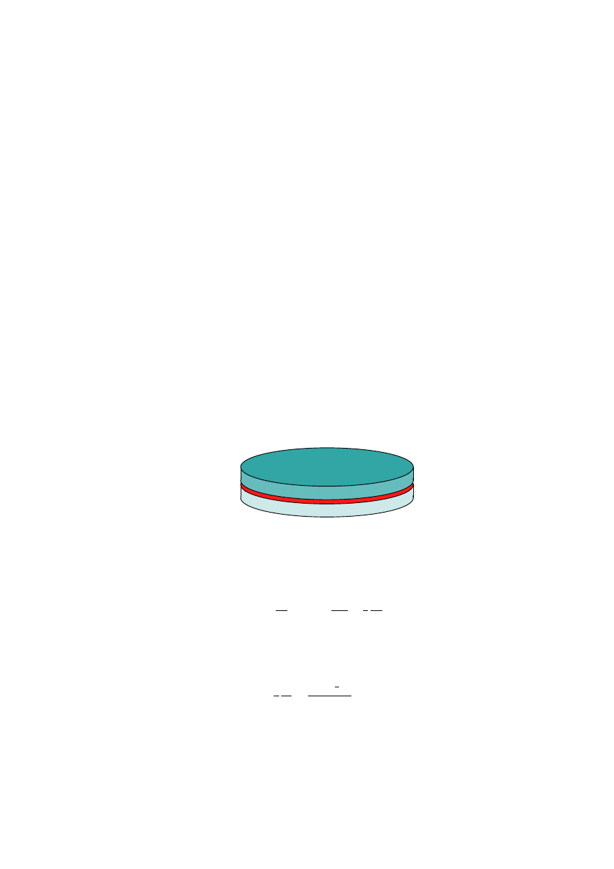
Chapter 10
Bessel functions and two-dimensional
problems
10.1
Temperature on a disk
Let us now turn to a different two-dimensional problem. A circular disk is prepared in such a way that its
initial temperature is radially symmetric,
u(ρ, φ, t = 0) = f (ρ).
(10.1)
Then it is placed between two perfect insulators and its circumference is connected to a freezer that keeps it
at 0
◦
C, as sketched in Fig. 10.2.
Figure 10.1: A circular plate, insulated from above and below.
Since the initial conditions do not depend on φ, we expect the solution to be radially symmetric as well,
u(ρ, t), which satisfies the equation
∂u
∂t
=
k
∂
2
u
∂ρ
2
+
1
ρ
∂u
∂ρ
,
u(c, t) = 0,
u(ρ, 0)
=
f (ρ).
(10.2)
Once again we separate variables, u(ρ, t) = R(ρ)T (t), which leads to the equation
1
k
T
0
T
=
R
00
+
1
ρ
R
0
R
=
−λ.
(10.3)
This corresponds to the two equations
ρ
2
R
00
+ ρR
0
+ λρ
2
R
=
0,
R(c) = 0m
T
0
+ λkT = 0.
(10.4)
61

62
CHAPTER 10. BESSEL FUNCTIONS
- 1
- 0.5
0
0.5
1
x
- 1
- 0.5
0
0.5
1
y
0
25
50
75
100
T
- 1
- 0.5
0
0.5
1
x
- 1
- 0.5
0
0.5
1
y
Figure 10.2: The initial temperature in the disk.
The radial equation (which has a regular singular point at ρ = 0) is closely related to one of the most important
equation of mathematical physics, Bessel’s equation. This equation can be reached from the substitution
ρ = x/
√
λ, so that with R(r) = X(x) we get the equation
x
2
d
2
dx
2
X(x) + x
d
dx
X(x) + x
2
X(x) = 0,
X(
√
λc) = 0.
(10.5)
10.2
Bessel’s equation
Bessel’s equation of order ν is given by
x
2
y
00
+ xy
0
+ (x
2
− ν
2
)y = 0.
(10.6)
Clearly x = 0 is a regular singular point, so we can solve by Frobenius’ method. The indicial equation is
obtained from the lowest power after the substitution y = x
γ
, and is
γ
2
− ν
2
= 0
(10.7)
So a generalised series solution gives two independent solutions if ν 6=
1
2
n. Now let us solve the problem and
explicitly substitute the power series,
y = x
ν
X
n
a
n
x
n
.
(10.8)
From Bessel’s equation we find
X
n
(n + ν)(n + ν − 1)a
ν
x
m+ν
+
X
n
(n + ν)a
ν
x
m+ν
+
X
n
(x
2
− ν
2
)a
ν
= 0
(10.9)
which leads to
[(m + ν)
2
− ν
2
]a
m
= −a
m−2
(10.10)
or
a
m
= −
1
m(m + 2ν)
a
m−2
.
(10.11)

10.2. BESSEL’S EQUATION
63
If we take ν = n > 0, we have
a
m
=
−
1
m(m + 2n)
a
m
−2
.
(10.12)
This can be solved by iteration,
a
2k
=
−
1
4
1
k(k + n)
a
2(k−1)
=
1
4
2
1
k(k − 1)(k + n)(k + n − 1)
a
2(k−2)
=
−
1
4
k
n!
k!(k + n)!
a
0
.
(10.13)
If we choose
1
a
0
=
1
n!2
n
we find the Bessel function of order n
J
n
(x) =
∞
X
k=0
(−1)
k
k!(k + n)!
x
2
2k+n
.
(10.14)
There is another second independent solution (which should have a logarithm in it) with goes to infinity at
x = 0.
0
2
4
6
8
10
x
−2
−1
0
1
y
J
0
J
1
J
2
Y
0
Y
1
Y
2
Figure 10.3: A plot of the first three Bessel functions J
n
and Y
n
.
The general solution of Bessel’s equation of order n is a linear combination of J and Y ,
y(x) = AJ
n
(x) + BY
n
(x).
(10.15)
1
This can be done since Bessel’s equation is linear, i.e., if g(x) is a solution Cg(x) is also a solution.

64
CHAPTER 10. BESSEL FUNCTIONS
10.3
Gamma function
For ν not an integer the recursion relation for the Bessel function generates something very similar to factorials.
These quantities are most easily expressed in something called a Gamma-function, defined as
Γ(ν) =
Z
∞
0
e
−t
t
ν
−1
dt,
ν > 0.
(10.16)
Some special properties of Γ function now follow immediately:
Γ(1)
=
Z
∞
0
e
−t
dt = −e
−1
∞
0
= 1 − e
−∞
= 1
Γ(ν)
=
Z
∞
0
e
−t
t
ν−1
dt = −
Z
∞
0
de
−t
dt
t
ν
−1
dt
=
−e
−t
t
ν−1
∞
0
+ (ν − 1)
Z
∞
0
e
−t
t
ν−2
dt
(10.17)
The first term is zero, and we obtain
Γ(ν) = (ν − 1)Γ(ν − 1)
(10.18)
From this we conclude that
Γ(2) = 1 · 1 = 1, Γ(3) = 2 · 1 · 1 = 2, Γ(4) = 3 · 2 · 1 · 1 = 2, Γ(n) = (n − 1)!.
(10.19)
Thus for integer argument the Γ function is nothing but a factorial, but it also defined for other arguments.
This is the sense in which Γ generalises the factorial to non-integer arguments. One should realize that once
one knows the Γ function between the values of its argument of, say, 1 and 2, one can evaluate any value of
the Γ function through recursion. Given that Γ(1.65) = 0.9001168163 we find
Γ(3.65) = 2.65
× 1.65 × 0.9001168163 = 3.935760779.
(10.20)
Question:
Evaluate Γ(3), Γ(11), Γ(2.65).
Answer:
2! = 2, 10! = 3628800, 1.65 × 0.9001168163 = 1.485192746.
We also would like to determine the Γ function for ν < 1. One can invert the recursion relation to read
Γ(ν − 1) =
Γ(ν)
ν − 1
,
(10.21)
Γ(0.7) = Γ(1.7)/0.7 = 0.909/0.7 = 1.30.
What is Γ(ν) for ν < 0? Let us repeat the recursion derived above and find
Γ(−1.3) =
Γ(−0.3)
−1.3
=
Γ(0.7)
−1.3 × −0.3
=
Γ(1.7)
0.7
× −0.3 × −1.3
= 3.33 .
(10.22)
This works for any value of the argument that is not an integer. If the argument is integer we get into problems.
Look at Γ(0). For small positive
Γ(±) =
Γ(1 ± )
±
= ±
1
→ ±∞.
(10.23)
Thus Γ(n) is not defined for n ≤ 0. This can be easily seen in the graph of the Γ function, Fig. 10.4.
Finally, in physical problems one often uses Γ(1/2),
Γ(
1
2
) =
Z
∞
0
e
−t
t
−1/2
dt = 2
Z
∞
0
e
−t
dt
1/2
= 2
Z
∞
0
e
−x
2
dx.
(10.24)
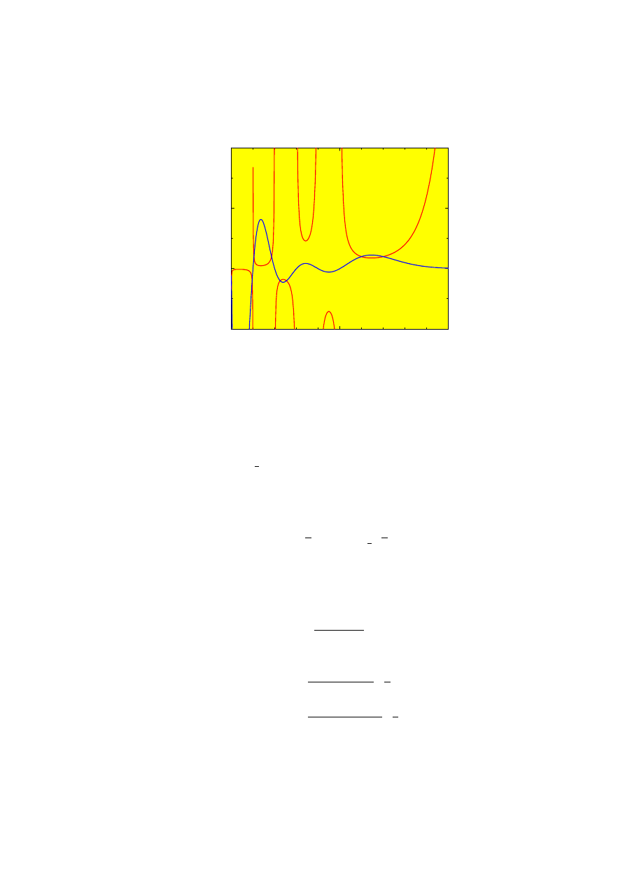
10.4. BESSEL FUNCTIONS OF GENERAL ORDER
65
−5
0
5
x
−5
0
5
10
Γ
(x)
Figure 10.4: A graph of the Γ function (solid line). The inverse 1/Γ is also included (dashed line). Note that
this last function is not discontinuous.
This can be evaluated by a very smart trick, we first evaluate Γ(1/2)
2
using polar coordinates
Γ(
1
2
)
2
= 4
Z
∞
0
e
−x
2
dx
Z
∞
0
e
−y
2
dy
= 4
Z
∞
0
Z
π/2
0
e
−ρ
2
ρdρdφ = π.
(10.25)
(See the discussion of polar coordinates in Sec. 7.1.) We thus find
Γ(1/2) =
√
π, Γ(3/2) =
1
2
√
π, etc.
(10.26)
10.4
Bessel functions of general order
The recurrence relation for the Bessel function of general order ±ν can now be solved by using the gamma
function,
a
m
= −
1
m(m ± 2ν)
a
m−2
(10.27)
has the solutions (x > 0)
J
ν
(x) =
∞
X
k=0
(−1)
k
k!Γ(ν + k + 1)
x
2
ν+2k
,
(10.28)
J
−ν
(x) =
∞
X
k=0
(−1)
k
k!Γ(−ν + k + 1)
x
2
−ν+2k
.
(10.29)
The general solution to Bessel’s equation of order ν is thus
y(x) = AJ
ν
(x) + BJ
−ν
(x),
(10.30)

66
CHAPTER 10. BESSEL FUNCTIONS
for any non-integer value of ν. This also holds for half-integer values (no logs).
10.5
Properties of Bessel functions
Bessel functions have many interesting properties:
J
0
(0) = 1,
(10.31)
J
ν
(x) = 0 (if ν > 0),
(10.32)
J
−n
(x) = (−1)
n
J
n
(x),
(10.33)
d
dx
x
−ν
J
ν
(x)
= −x
−ν
J
ν+1
(x),
(10.34)
d
dx
[x
ν
J
ν
(x)] = x
ν
J
ν
−1
(x),
(10.35)
d
dx
[J
ν
(x)] =
1
2
[J
ν
−1
(x) − J
ν+1
(x)] ,
(10.36)
xJ
ν+1
(x) =
2νJ
ν
(x) − xJ
ν−1
(x),
(10.37)
Z
x
−ν
J
ν+1
(x) dx = −x
−ν
J
ν
(x) + C,
(10.38)
Z
x
ν
J
ν−1
(x) dx = x
ν
J
ν
(x) + C.
(10.39)
Let me prove a few of these. First notice from the definition that J
n
(x) is even or odd if n is even or odd,
J
n
(x) =
∞
X
k=0
(−1)
k
k!(n + k)!
x
2
n+2k
.
(10.40)
Substituting x = 0 in the definition of the Bessel function gives 0 if ν > 0, since in that case we have the sum
of positive powers of 0, which are all equally zero.
Let’s look at J
−n
:
J
−n
(x) =
∞
X
k=0
(
−1)
k
k!Γ(−n + k + 1)!
x
2
n+2k
=
∞
X
k=n
(−1)
k
k!Γ(−n + k + 1)!
x
2
−n+2k
=
∞
X
l=0
(
−1)
l+n
(l + n)!l!
x
2
n+2l
=
(−1)
n
J
n
(x).
(10.41)
Here we have used the fact that since Γ(
−l) = ±∞, 1/Γ(−l) = 0 [this can also be proven by defining a
recurrence relation for 1/Γ(l)]. Furthermore we changed summation variables to l = −n + k.

10.6. STURM-LIOUVILLE THEORY
67
The next one:
d
dx
x
−ν
J
ν
(x)
= 2
−ν
d
dx
(
∞
X
k=0
(
−1)
k
k!Γ(ν + k + 1)
x
2
2k
)
=
2
−ν
∞
X
k=1
(−1)
k
(k − 1)!Γ(ν + k + 1)
x
2
2k−1
=
−2
−ν
∞
X
l=0
(−1)
l
(l)!Γ(ν + l + 2)
x
2
2l+1
=
−2
−ν
∞
X
l=0
(
−1)
l
(l)!Γ(ν + 1 + l + 1)
x
2
2l+1
= −x
−ν
∞
X
l=0
(−1)
l
(l)!Γ(ν + 1 + l + 1)
x
2
2l+ν+1
=
−x
−ν
J
ν+1
(x).
(10.42)
Similarly
d
dx
[x
ν
J
ν
(x)] =
x
ν
J
ν−1
(x).
(10.43)
The next relation can be obtained by evaluating the derivatives in the two equations above, and solving
for J
ν
(x):
x
−ν
J
0
ν
(x)
− νx
−ν−1
J
ν
(x) = −x
−ν
J
ν+1
(x),
(10.44)
x
ν
J
ν
(x) + νx
ν−1
J
ν
(x) =
x
ν
J
ν
−1
(x).
(10.45)
Multiply the first equation by x
ν
and the second one by x
−ν
and add:
−2ν
1
x
J
ν
(x) = −J
ν+1
(x) + J
ν−1
(x).
(10.46)
After rearrangement of terms this leads to the desired expression.
Eliminating J
ν
between the equations gives (same multiplication, take difference instead)
2J
0
ν
(x)
=
J
ν+1
(x) + J
ν−1
(x).
(10.47)
Integrating the differential relations leads to the integral relations.
Bessel function are an inexhaustible subject – there are always more useful properties than one knows. In
mathematical physics one often uses specialist books.
10.6
Sturm-Liouville theory
In the end we shall want to write a solution to an equation as a series of Bessel functions. In order to do that
we shall need to understand about orthogonality of Bessel function – just as sines and cosines were orthogonal.
This is most easily done by developing a mathematical tool called Sturm-Liouville theory. It starts from an
equation in the so-called self-adjoint form
[r(x)y
0
(x)]
0
+ [p(x) + λs(x)]y(x) = 0
(10.48)
where λ is a number, and r(x) and s(x) are greater than 0 on [a, b]. We apply the boundary conditions
a
1
y(a) + a
2
y
0
(a) = 0,
b
1
y(b) + b
2
y
0
(b) = 0,
(10.49)
with a
1
and a
2
not both zero, and b
1
and b
2
similar.
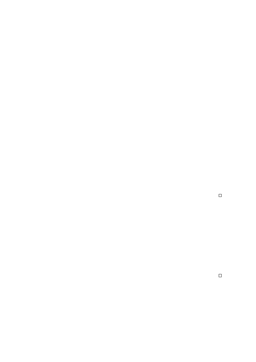
68
CHAPTER 10. BESSEL FUNCTIONS
Theorem 1. If there is a solution to (10.48) then λ is real.
Proof. Assume that λ is a complex number (λ = α + iβ) with solution Φ. By complex conjugation we find
that
[r(x)Φ
0
(x)]
0
+ [p(x) + λs(x)]Φ(x) =
0
[r(x)(Φ
∗
)
0
(x)]
0
+ [p(x) + λ
∗
s(x)](Φ
∗
)(x) =
0
(10.50)
where ∗ note complex conjugation. Multiply the first equation by Φ
∗
(x) and the second by Φ(x), and subtract
the two equations:
(λ
∗
− λ)s(x)Φ
∗
(x)Φ(x) = Φ(x)[r(x)(Φ
∗
)
0
(x)]
0
− Φ
∗
(x)[r(x)Φ
0
(x)]
0
.
(10.51)
Now integrate over x from a to b and find
(λ
∗
− λ)
Z
b
a
s(x)Φ
∗
(x)Φ(x) dx =
Z
b
a
Φ(x)[r(x)(Φ
∗
)
0
(x)]
0
− Φ
∗
(x)[r(x)Φ
0
(x)]
0
dx
(10.52)
The second part can be integrated by parts, and we find
(λ
∗
− λ)
Z
b
a
s(x)Φ
∗
(x)Φ(x) dx
= [Φ
0
(x)r(x)(Φ
∗
)
0
(x) − Φ
∗
(x)r(x)Φ
0
(x)
|
b
a
=
r(b) [Φ
0
(b)(Φ
∗
)
0
(b) − Φ
∗
(b)Φ
0
(b)]
−r(a) [Φ
0
(a)(Φ
∗
)
0
(a) − Φ
∗
(a)Φ
0
(a)]
= 0,
(10.53)
where the last step can be done using the boundary conditions. Since both Φ
∗
(x)Φ(x) and s(x) are greater
than zero we conclude that
R
b
a
s(x)Φ
∗
(x)Φ(x) dx > 0, which can now be divided out of the equation to lead to
λ = λ
∗
.
Theorem 2. Let Φ
n
and Φ
m
be two solutions for different values of λ, λ
n
6= λ
m
, then
Z
b
a
s(x)Φ
n
(x)Φ
m
(x) dx = 0.
(10.54)
Proof. The proof is to a large extent identical to the one above: multiply the equation for Φ
n
(x) by Φ
m
(x)
and vice-versa. Subtract and find
(λ
n
− λ
m
)
Z
b
a
s(x)Φ
m
(x)Φ
n
(x) dx = 0
(10.55)
which leads us to conclude that
Z
b
a
s(x)Φ
n
(x)Φ
m
(x) dx = 0.
(10.56)
Theorem 3. Under the conditions set out above
a) There exists a real infinite set of eigenvalues λ
0
, . . . , λ
n
, . . . with lim
n→∞
= ∞.
b)If Φ
n
is the eigenfunction corresponding to λ
n
, it has exactly n zeroes in [a, b]. No proof shall be given.
Clearly the Bessel equation is of self-adjoint form: rewrite
x
2
y
00
+ xy
0
+ (x
2
− ν
2
)y = 0
(10.57)

10.7. OUR INITIAL PROBLEM AND BESSEL FUNCTIONS
69
as (divide by x)
[xy
0
]
0
+ (x −
ν
2
x
)y = 0
(10.58)
We cannot identify ν with λ, and we do not have positive weight functions. It can be proven from properties
of the equation that the Bessel functions have an infinite number of zeroes on the interval [0, ∞). A small list
of these:
J
0
:
2.42
5.52
8.65
11.79
. . .
J
1/2
: π
2π
3π
4π
. . .
J
8
: 11.20 16.04 19.60 22.90 . . .
(10.59)
10.7
Our initial problem and Bessel functions
We started the discussion from the problem of the temperature on a circular disk, solved in polar coordinates,
Since the initial conditions do not depend on φ, we expect the solution to be radially symmetric as well, u(ρ, t),
which satisfies the equation
∂u
∂t
=
k
∂
2
u
∂ρ
2
+
1
ρ
∂u
∂ρ
,
u(c, t) = 0,
u(ρ, 0)
=
f (ρ).
(10.60)
With u(ρ, t) = R(ρ)T (t) we found the equations
ρ
2
R
00
+ ρR
0
+ λρ
2
R
= 0
R(c) = 0
T
0
+ λkT = 0.
(10.61)
The equation for R is clearly self-adjoint, it can be written as
[ρR
0
]
0
+ λρR = 0
(10.62)
So how does the equation for R relate to Bessel’s equation? Let us make the change of variables x =
√
λρ.
We find
d
dρ
=
√
λ
d
dx
,
(10.63)
and we can remove a common factor
√
λ to obtain (X(x) = R(ρ))
[xX
0
]
0
+ xX = 0,
(10.64)
which is Bessel’s equation of order 0, i.e.,
R(ρ) = J
0
(ρ
√
λ).
(10.65)
The boundary condition R(c) = 0 shows that
c
p
λ
n
= x
n
,
(10.66)
where x
n
are the points where J
0
(x) = 0. We thus conclude
R
n
(ρ) = J
0
(ρ
p
λ
n
).
(10.67)
the first five solutions R
n
(for c = 1) are shown in Fig. 10.5.
From Sturm-Liouville theory we conclude that
Z
∞
0
ρdρ R
n
(ρ)R
m
(ρ) = 0 if n
6= m.
(10.68)

70
CHAPTER 10. BESSEL FUNCTIONS
0.2
0.4
0.6
0.8
1
x
- 0.4
- 0.2
0.2
0.4
0.6
0.8
1
R
Figure 10.5: A graph of the first five functions R
n
Together with the solution for the T equation,
T
n
(t) = exp(−λ
n
kt)
(10.69)
we find a Fourier-Bessel series type solution
u(ρ, t) =
∞
X
n=1
A
n
J
0
(ρ
p
λ
n
) exp(−λ
n
kt),
(10.70)
with λ
n
= (x
n
/c)
2
.
In order to understand how to determine the coefficients A
n
from the initial condition u(ρ, 0) = f (ρ) we
need to study Fourier-Bessel series in a little more detail.
10.8
Fourier-Bessel series
So how can we determine in general the coefficients in the Fourier-Bessel series
f (ρ) =
∞
X
j=1
C
j
J
ν
(α
j
ρ)?
(10.71)
The corresponding self-adjoint version of Bessel’s equation is easily found to be (with R
j
(ρ) = J
ν
(α
j
ρ))
(ρR
0
j
)
0
+ (α
2
j
ρ −
ν
2
ρ
)R
j
= 0.
(10.72)
Where we assume that f and R satisfy the boundary condition
b
1
f (c) + b
2
f
0
(c) = 0
b
1
R
j
(c) + b
2
R
0
j
(c)
=
0
(10.73)
From Sturm-Liouville theory we do know that
Z
c
0
ρJ
ν
(α
i
ρ)J
ν
(α
j
ρ) = 0 if i 6= j,
(10.74)

10.8. FOURIER-BESSEL SERIES
71
but we shall also need the values when i = j!
Let us use the self-adjoint form of the equation, and multiply with 2ρR
0
, and integrate over ρ from 0 to c,
Z
c
0
(ρR
0
j
)
0
+ (α
2
j
ρ −
ν
2
ρ
)R
j
2ρR
0
j
dρ = 0.
(10.75)
This can be brought to the form (integrate the first term by parts, bring the other two terms to the right-hand
side)
Z
c
0
d
dρ
ρR
0
j
2
dρ
=
2ν
2
Z
c
0
R
j
R
0
j
dρ
− 2α
2
j
Z
c
0
ρ
2
R
j
R
0
j
dρ
(10.76)
ρR
0
j
2
c
0
=
ν
2
R
2
j
c
0
− 2α
2
j
Z
c
0
ρ
2
R
j
R
0
j
dρ.
(10.77)
The last integral can now be done by parts:
2
Z
c
0
ρ
2
R
j
R
0
j
dρ
=
−2
Z
c
0
ρR
2
j
dρ + ρR
2
j
c
0
.
(10.78)
So we finally conclude that
2α
2
j
Z
c
0
ρR
2
j
dρ =
h
α
2
j
ρ
2
− ν
2
R
2
j
+
ρR
0
j
2
c
0
.
(10.79)
In order to make life not too complicated we shall only look at boundary conditions where f (c) = R(c) = 0.
The other cases (mixed or purely f
0
(c) = 0) go very similar! Using the fact that R
j
(r) = J
ν
(α
j
ρ), we find
R
0
j
= α
j
J
0
ν
(α
j
ρ).
(10.80)
We conclude that
2α
2
j
Z
c
0
ρ
2
R
2
j
dρ
=
h
(ρα
j
J
0
ν
(α
j
ρ))
2
c
0
=
c
2
α
2
j
(J
0
ν
(α
j
c))
2
= c
2
α
2
j
ν
α
j
c
J
ν
(α
j
c) − J
ν+1
(α
j
c)
2
=
c
2
α
2
j
(J
ν+1
(α
j
c))
2
,
(10.81)
We thus finally have the result
Z
c
0
ρ
2
R
2
j
dρ =
c
2
2
J
2
ν+1
(α
j
c).
(10.82)
Example 10.1:
Consider the function
f (x) =
x
3
0 < x < 10
0
x > 10
(10.83)
Expand this function in a Fourier-Bessel series using J
3
.
Solution:
From our definitions we find that
f (x) =
∞
X
j=1
A
j
J
3
(α
j
x),
(10.84)

72
CHAPTER 10. BESSEL FUNCTIONS
with
A
j
=
2
100J
4
(10α
j
)
2
Z
10
0
x
3
J
3
(α
j
x)dx
=
2
100J
4
(10α
j
)
2
1
α
5
j
Z
10α
j
0
s
4
J
3
(s)ds
=
2
100J
4
(10α
j
)
2
1
α
5
j
(10α
j
)
4
J
4
(10α
j
)ds
=
200
α
j
J
4
(10α
j
)
.
(10.85)
Using α
j
= . . ., we find that the first five values of A
j
are 1050.95, −821.503, 703.991, −627.577, 572.301.
The first five partial sums are plotted in Fig. 10.6.
2
4
6
8
10
x
200
400
600
800
f
Figure 10.6: A graph of the first five partial sums for x
3
expressed in J
3
.
10.9
Back to our initial problem
After all that we have learned, we know that in order to determine the solution of the initial problem in Sec.
10.1 we would have to calculate the integrals
A
j
=
2
c
2
J
2
1
(cα
j
)
Z
c
0
f (ρ)J
0
(α
j
ρ)ρdρ
(10.86)

Chapter 11
Separation of variables in three
dimensions
We have up to now concentrated on 2D problems, but a lot of physics is three dimensional, and often we
have spherical symmetry – that means symmetry for rotation over any angle. In these cases we use spherical
coordinates, as indicated in figure 7.3.
11.1
Modelling the eye
z-axis
Figure 11.1: The temperature in a simple model of the eye
Let me model the temperature in a simple model of the eye, where the eye is a sphere, and the eyelids are
circular. In that case we can put the z-axis straight through the middle of the eye, and we can assume that
the temperature does only depend on r, θ and not on φ. We assume that the part of the eye in contact with
air is at a temperature of 20
◦
C, and the part in contact with the body is at 36
◦
C. If we look for the steady
state temperature it is described by Laplace’s equation,
∇
2
u(r, θ) = 0.
(11.1)
73

74
CHAPTER 11. SEPARATION OF VARIABLES IN THREE DIMENSIONS
Expressing the Laplacian
∇
2
in spherical coordinates (see chapter 7) we find
1
r
2
∂
∂r
r
2
∂u
∂r
+
1
r
2
sin θ
∂
∂θ
sin θ
∂u
∂θ
= 0.
(11.2)
Once again we solve the equation by separation of variables,
u(r, θ) = R(r)T (θ).
(11.3)
After this substitution we realize that
[r
2
R
0
]
0
R
= −
[sin θT
0
]
0
T sin θ
= λ.
(11.4)
The equation for R will be shown to be easy to solve (later). The one for T is of much more interest. Since
for 3D problems the angular dependence is more complicated, whereas in 2D the angular functions were just
sines and cosines.
The equation for T is
[sin θT
0
]
0
+ λT sin θ = 0.
(11.5)
This equation is called Legendre’s equation, or actually it carries that name after changing variables to x =
cos θ. Since θ runs from 0 to π, we find sin θ > 0, and we have
sin θ =
p
1 − x
2
.
(11.6)
After this substitution we are making the change of variables we find the equation (y(x) = T (θ) =
T (arccos x), and we now differentiate w.r.t. x, d/dθ = −
√
1 − x
2
d/dx)
d
dx
(1
− x
2
)
dy
dx
+ λy = 0.
(11.7)
This equation is easily seen to be self-adjoint. It is not very hard to show that x = 0 is a regular (not singular)
point – but the equation is singular at x = ±1. Near x = 0 we can solve it by straightforward substitution of
a Taylor series,
y(x) =
X
j=0
a
j
x
j
.
(11.8)
We find the equation
∞
X
j=0
j(j − 1)a
j
x
j
−2
−
∞
X
j=0
j(j
− 1)a
j
x
j
− 2
∞
X
j=0
ja
j
x
j
+ λ
∞
X
j=0
a
j
x
j
= 0
(11.9)
After introducing the new variable i = j − 2, we have
∞
X
j=0
(i + 1)(i + 1)a
i+2
x
i
−
∞
X
j=0
[j(j + 1)
− λ]a
j
x
j
= 0.
(11.10)
Collecting the terms of the order x
k
, we find the recurrence relation
a
k+2
=
k(k + 1) − λ
(k + 1)(k + 2)
a
k
.
(11.11)
If λ = n(n + 1) this series terminates – actually those are the only acceptable solutions, any one where λ takes
a different value actually diverges at x = +1 or x = −1, not acceptable for a physical quantity – it can’t just
diverge at the north or south pole (x = cos θ = ±1 are the north and south pole of a sphere).

11.2. PROPERTIES OF LEGENDRE POLYNOMIALS
75
We thus have, for n even,
y
n
= a
0
+ a
2
x
2
+ . . . + a
n
x
n
.
(11.12)
For odd n we find odd polynomials,
y
n
= a
1
x + a
3
x
3
+ . . . + a
n
x
n
.
(11.13)
One conventionally defines
a
n
=
(2n)!
n!
2
2
n
.
(11.14)
With this definition we obtain
P
0
=
1,
P
1
=
x,
P
2
=
3
2
x
2
−
1
2
,
P
3
=
1
2
(5x
3
− 3x),
P
4
=
1
8
(35x
4
− 30x
2
+ 3),
P
5
=
1
8
(63x
5
− 70x
3
+ 15x).
(11.15)
A graph of these polynomials can be found in figure 11.2.
−1
0
1
x
−1
0
1
P
n
(x)
n=0
n=1
n=2
n=3
n=4
n=5
Figure 11.2: The first few Legendre polynomials P
n
(x).
11.2
Properties of Legendre polynomials
11.2.1
Generating function
Let F (x, t) be a function of the two variables x and t that can be expressed as a Taylor’s series in t,
P
n
c
n
(x)t
n
.
The function F is then called a generating function of the functions c
n
.
Example 11.1:
Show that F (x, t) =
1
1
−xt
is a generating function of the polynomials x
n
.
Solution:
Look at
1
1 − xt
=
∞
X
n=0
x
n
t
n
(|xt| < 1).
(11.16)

76
CHAPTER 11. SEPARATION OF VARIABLES IN THREE DIMENSIONS
Example 11.2:
Show that F (x, t) = exp
tx−t
2t
is the generating function for the Bessel functions,
F (x, t) = exp(
tx
− t
2t
) =
∞
X
n=0
J
n
(x)t
n
.
(11.17)
Example 11.3:
(The case of most interest here)
F (x, t) =
1
√
1 − 2xt + t
2
=
∞
X
n=0
P
n
(x)t
n
.
(11.18)
11.2.2
Rodrigues’ Formula
P
n
(x) =
1
2
n
n!
d
n
dx
n
(x
2
− 1)
n
.
(11.19)
11.2.3
A table of properties
1. P
n
(x) is even or odd if n is even or odd.
2. P
n
(1) = 1.
3. P
n
(
−1) = (−1)
n
.
4. (2n + 1)P
n
(x) = P
0
n+1
(x) − P
0
n−1
(x).
5. (2n + 1)xP
n
(x) = (n + 1)P
n+1
(x) + nP
n
−1
(x).
6.
R
x
−1
P
n
(x
0
)dx
0
=
1
2n+1
[P
n+1
(x) − P
n
−1
(x)].
Let us prove some of these relations, first Rodrigues’ formula. We start from the simple formula
(x
2
− 1)
d
dx
(x
2
− 1)
n
− 2nx(x
2
− 1)
n
= 0,
(11.20)
which is easily proven by explicit differentiation. This is then differentiated n + 1 times,
d
n+1
dx
n+1
(x
2
− 1)
d
dx
(x
2
− 1)
n
− 2nx(x
2
− 1)
n
=
n(n + 1)
d
n
dx
n
(x
2
− 1)
n
+ 2(n + 1)x
d
n+1
dx
n+1
(x
2
− 1)
n
+ (x
2
− 1)
d
n+2
dx
n+2
(x
2
− 1)
n
−2n(n + 1)
d
n
dx
n
(x
2
− 1)
n
− 2nx
d
n+1
dx
n+1
(x
2
− 1)
n
=
−n(n + 1)
d
n
dx
n
(x
2
− 1)
n
+ 2x
d
n+1
dx
n+1
(x
2
− 1)
n
+ (x
2
− 1)
d
n+2
dx
n+2
(x
2
− 1)
n
=
−
d
dx
(1 − x
2
)
d
dx
d
n
dx
n
(x
2
− 1)
n
+ n(n + 1)
d
n
dx
n
(x
2
− 1)
n
= 0.
(11.21)
We have thus proven that
d
n
dx
n
(x
2
− 1)
n
satisfies Legendre’s equation. The normalisation follows from the
evaluation of the highest coefficient,
d
n
dx
n
x
2n
=
2n!
n!
x
n
,
(11.22)

11.3. FOURIER-LEGENDRE SERIES
77
and thus we need to multiply the derivative with
1
2
n
n!
to get the properly normalised P
n
.
Let’s use the generating function to prove some of the other properties: 2.:
F (1, t) =
1
1 − t
=
X
n
t
n
(11.23)
has all coefficients one, so P
n
(1) = 1. Similarly for 3.:
F (−1, t) =
1
1 + t
=
X
n
(−1)
n
t
n
.
(11.24)
Property 5. can be found by differentiating the generating function with respect to t:
d
dt
1
√
1 − 2tx + t
2
=
d
dt
∞
X
n=0
t
n
P
n
(x)
x − t
(1 − 2tx + t
2
)
3/2
=
X
n=0
nt
n−1
P
n
(x)
x − t
1 − 2xt + t
2
∞
X
n=0
t
n
P
n
(x)
=
X
n=0
nt
n
−1
P
n
(x)
∞
X
n=0
t
n
xP
n
(x)
−
∞
X
n=0
t
n+1
P
n
(x)
=
∞
X
n=0
nt
n−1
P
n
(x) − 2
∞
X
n=0
nt
n
xP
n
(x) +
∞
X
n=0
nt
n+1
P
n
(x)
∞
X
n=0
t
n
(2n + 1)xP
n
(x) =
∞
X
n=0
(n + 1)t
n
P
n+1
(x) +
∞
X
n=0
nt
n
P
n−1
(x)
(11.25)
Equating terms with identical powers of t we find
(2n + 1)xP
n
(x) = (n + 1)P
n+1
(x) + nP
n
−1
(x).
(11.26)
Proofs for the other properties can be found using similar methods.
11.3
Fourier-Legendre series
Since Legendre’s equation is self-adjoint, we can show that P
n
(x) forms an orthogonal set of functions. To
decompose functions as series in Legendre polynomials we shall need the integrals
Z
1
−1
P
2
n
(x)dx =
2n + 1
2
,
(11.27)
which can be determined using the relation 5. twice to obtain a recurrence relation
Z
1
−1
P
2
n
(x)dx =
Z
1
−1
P
n
(x)
(2n
− 1)xP
n
−1
(x) − (n − 1)P
n−2
(x)
n
dx
=
(2n − 1)
n
Z
1
−1
xP
n
(x)P
n−1
(x)dx
=
(2n − 1)
n
Z
1
−1
(n + 1)P
n+1
(x) + nP
n−1
(x)
2n + 1
P
n−1
(x)dx
=
(2n
− 1)
2n + 1
Z
1
−1
P
2
n
−1
(x)dx,
(11.28)

78
CHAPTER 11. SEPARATION OF VARIABLES IN THREE DIMENSIONS
and the use of a very simple integral to fix this number for n = 0,
Z
1
−1
P
2
0
(x)dx = 2.
(11.29)
So we can now develop any function on [−1, 1] in a Fourier-Legendre series
f (x) =
X
n
A
n
P
n
(x)
A
n
=
2n + 1
2
Z
1
−1
f (x)P
n
(x)dx
(11.30)
Example 11.4:
Find the Fourier-Legendre series for
f (x) =
0,
−1 < x < 0
1, 0 < x < 1
.
(11.31)
Solution:
We find
A
0
=
1
2
Z
1
0
P
0
(x)dx =
1
2
,
(11.32)
A
1
=
3
2
Z
1
0
P
1
(x)dx =
1
4
,
(11.33)
A
2
=
5
2
Z
1
0
P
2
(x)dx = 0,
(11.34)
A
3
=
7
2
Z
1
0
P
3
(x)dx = −
7
16
.
(11.35)
All other coefficients for even n are zero, for odd n they can be evaluated explicitly.
11.4
Modelling the eye–revisited
Let me return to my model of the eye. With the functions P
n
(cos θ) as the solution to the angular equation,
we find that the solutions to the radial equation are
R = Ar
n
+ Br
−n−1
.
(11.36)
The singular part is not acceptable, so once again we find that the solution takes the form
u(r, θ) =
∞
X
n=0
A
n
r
n
P
n
(cos θ)
(11.37)
We now need to impose the boundary condition that the temperature is 20
◦
C in an opening angle of 45
◦
, and
36
◦
elsewhere. This leads to the equation
∞
X
n=0
A
n
c
n
P
n
(cos θ) =
20 0 < θ < π/4
36
π/4 < θ < π
(11.38)
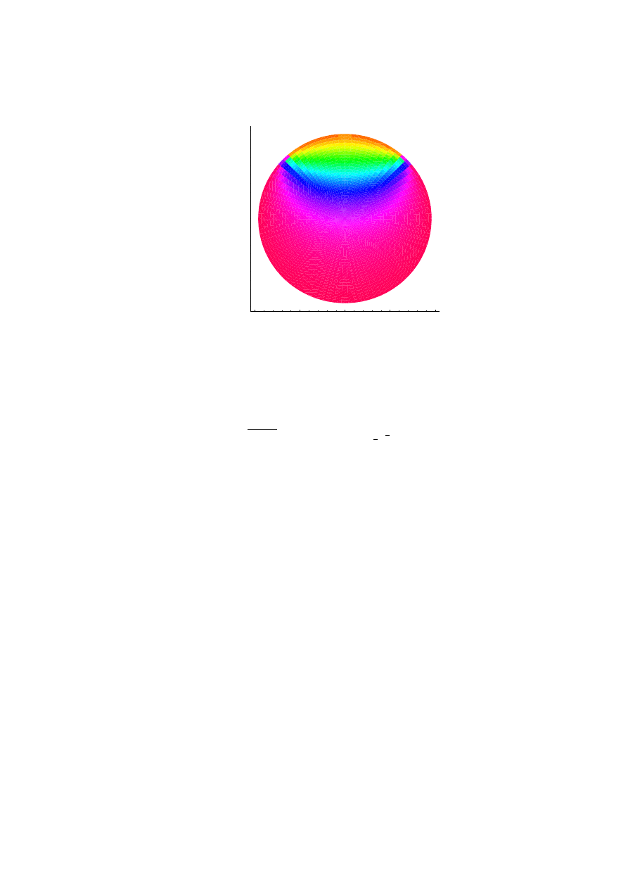
11.4. MODELLING THE EYE–REVISITED
79
-1
-0.5
0
0.5
1
-1
-0.5
0
0.5
1
-1
-0.5
0
0.5
1
Figure 11.3: A cross-section of the temperature in the eye. We have summed over the first 40 Legendre
polynomials.
This leads to the integral, after once again changing to x = cos θ,
A
n
=
2n + 1
2
"Z
1
−1
36P
n
(x)dx −
Z
1
1
2
√
2
16P
n
(x)dx
#
.
(11.39)
These integrals can easily be evaluated, and a sketch for the temperature can be found in figure 11.3.
Notice that we need to integrate over x = cos θ to obtain the coefficients A
n
. The integration over θ in
spherical coordinates is
R
π
0
sin θdθ =
R
1
−1
1dx, and so automatically implies that cos θ is the right variable to
use, as also follows from the orthogonality of P
n
(x).
Wyszukiwarka
Podobne podstrony:
Rajeev S G Advanced classical mechanics chaos (Rochester lecture notes, web draft, 2002)(100s) PCtm
Freitag Several complex variables local theory (lecture notes, web draft, 2001)(74s) MCc
Lugo G Differential geometry and physics (lecture notes, web draft, 2006)(61s) MDdg
Gardner Differential geometry and relativity (lecture notes, web draft, 2004) (198s) PGr
Rajeev S G Geometrical methods in physics (lecture notes, web draft, 2004)(97s)
Walet N Mathematics for Physicists (web draft, 2002)(81s) MCet
Dynkin E B Superdiffusions and Positive Solutions of Nonlinear PDEs (web draft,2005)(108s) MCde
Reid H Solved problems from Peskin Schroeder QFT, chapters 2 to 5 (web draft, 2002)(40s) PQft
Radulescu V D Nonlinear PDEs of elliptic type (math AP 0502173, web draft, 2005)(114s) MCde
Seahra S Path integrals in quantum field theory (web draft, 2002)(36s) PQft
Ziming Li Lecture notes on computer algebra (web draft, 2004)(31s) CsCa
Amendola L Dark energy (Heidelberg lectures, web draft, 2005)(43s) PGrc
Baez J , Smith B , Wise D Lectures on classical mechanics (web draft, 2005)(76s) PCtm
Athanassopoulos K Notes on symplectic geometry (Univ of Crete, web draft, 2007)(66s) MDdg
Neumann W D Notes on geometry and 3 manifolds, with appendices by P Norbury (web draft, 2004)(54s)
algorithms lecture notes
cis581 lecture notes chapter6
Pillay Lecture notes on Model theory (2002)
więcej podobnych podstron