
DIFFERENTIABLE MANIFOLDS
Section c course 2003
Nigel Hitchin
hitchin@maths.ox.ac.uk
1
1
Introduction
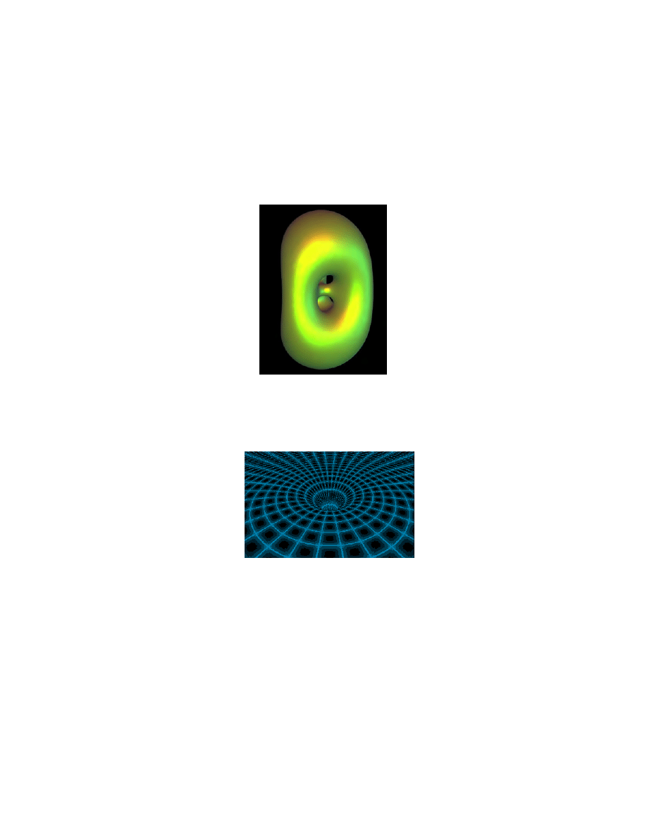
This is an introductory course on differentiable manifolds. These are higher dimen-
sional analogues of surfaces like this:
This is the image to have, but we shouldn’t think of a manifold as always sitting
inside a fixed Euclidean space like this one, but rather as an abstract object. One of
the historical driving forces of the theory was General Relativity, where the manifold
is four-dimensional spacetime, wormholes and all:
Spacetime is not part of a bigger Euclidean space, it just exists, but we need to learn
how to do analysis on it, which is what this course is about.
Another input to the subject is from mechanics – the dynamics of complicated me-
chanical systems involve spaces with many degrees of freedom. Just think of the
different configurations that an Anglepoise lamp can be put into:
2
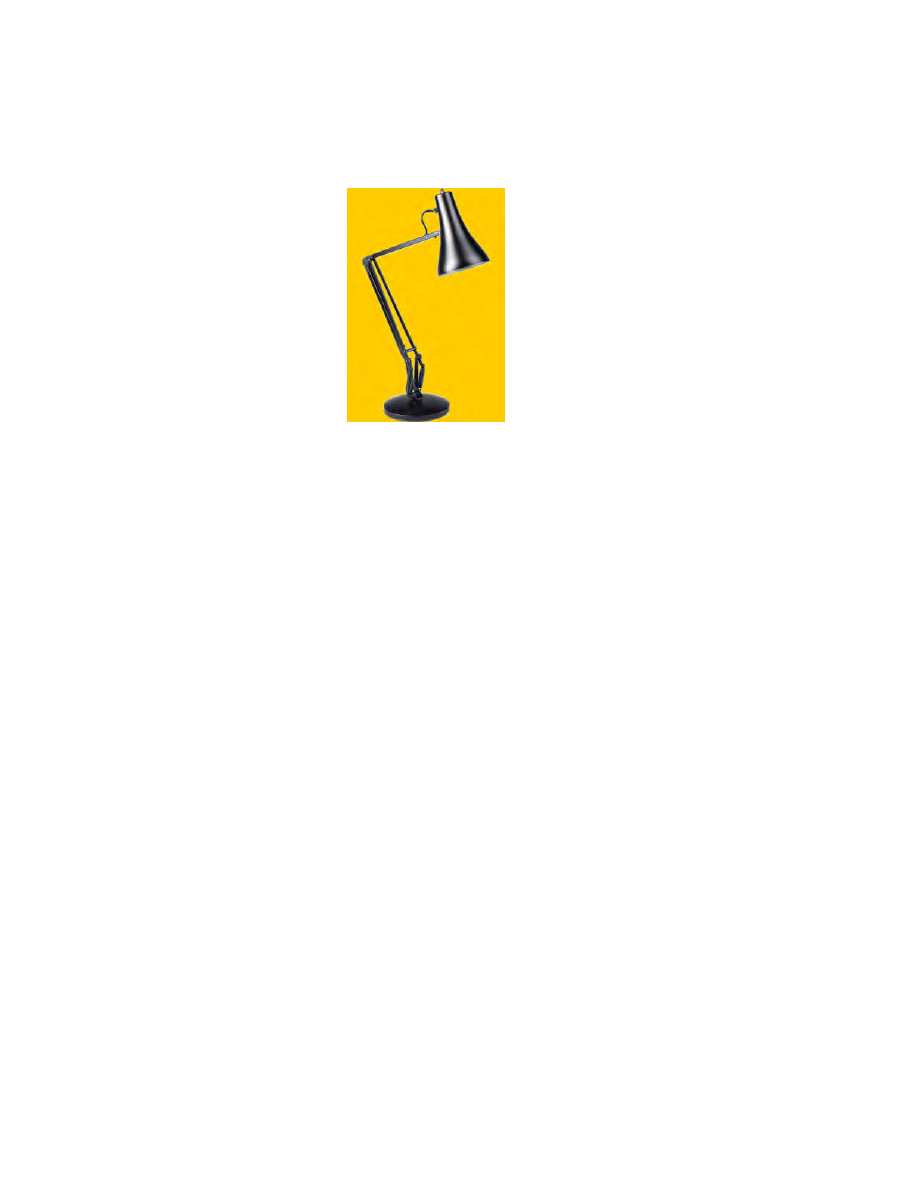
How many degrees of freedom are there? How do we describe the dynamics of this if
we hit it?
The first idea we shall meet is really the defining property of a manifold – to be able
to describe points locally by n real numbers, local coordinates. Then we shall need
to define analytical objects (vector fields, differential forms for example) which are
independent of the choice of coordinates. This has a double advantage: on the one
hand it enables us to discuss these objects on topologically non-trivial manifolds like
spheres, and on the other it also provides the language for expressing the equations
of mathematical physics in a coordinate-free form, one of the fundamental principles
of relativity.
The most basic example of analytical techniques on a manifold is the theory of dif-
ferential forms and the exterior derivative. This generalizes the grad, div and curl of
ordinary three-dimensional calculus. A large part of the course will be occupied with
this. It provides a very natural generalization of the theorems of Green and Stokes
in three dimensions and also gives rise to de Rham cohomology which is an analytical
way of approaching the algebraic topology of the manifold. This has been important
in an enormous range of areas from algebraic geometry to theoretical physics.
More refined use of analysis requires extra data on the manifold and we shall simply
define and describe some basic features of Riemannian metrics. These generalize
the first fundamental form of a surface and, in their Lorentzian guise, provide the
substance of general relativity. A more complete story demands a much longer course,
but here we shall consider just two aspects which draw on the theory of differential
forms: the study of geodesics via a vector field, the geodesic flow, on the cotangent
bundle, and some basic properties of harmonic forms.
Certain standard technical results which we shall require are proved in the Appendix
3

so as not to interrupt the development of the theory.
A good book to accompany the course is: An Introduction to Differential Manifolds
by Dennis Barden and Charles Thomas (Imperial College Press £19 (paperback)).
2
Manifolds
2.1
Coordinate charts
The concept of a manifold is a bit complicated, but it starts with defining the notion
of a coordinate chart.
Definition 1 A
coordinate chart
on a set X is a subset U ⊆ X together with a
bijection
ϕ : U → ϕ(U ) ⊆ R
n
onto an open set ϕ(U ) in R
n
.
Thus we can parametrize points of U by n coordinates ϕ(x) = (x
1
, . . . , x
n
).
We now want to consider the situation where X is covered by such charts and satisfies
some consistency conditions. We have
Definition 2 An n-dimensional
atlas
on X is a collection of coordinate charts {U
α
, ϕ
α
}
α∈I
such that
• X is covered by the {U
α
}
α∈I
• for each α, β ∈ I, ϕ
α
(U
α
∩ U
β
) is open in R
n
• the map
ϕ
β
ϕ
−1
α
: ϕ
α
(U
α
∩ U
β
) → ϕ
β
(U
α
∩ U
β
)
is C
∞
with C
∞
inverse.
Recall that F (x
1
, . . . , x
n
) ∈ R
n
is C
∞
if it has derivatives of all orders. We shall also
say that F is smooth in this case. It is perfectly possible to develop the theory of
manifolds with less differentiability than this, but this is the normal procedure.
4
Examples:
1. Let X = R
n
and take U = X with ϕ = id. We could also take X to be any open
set in R
n
.
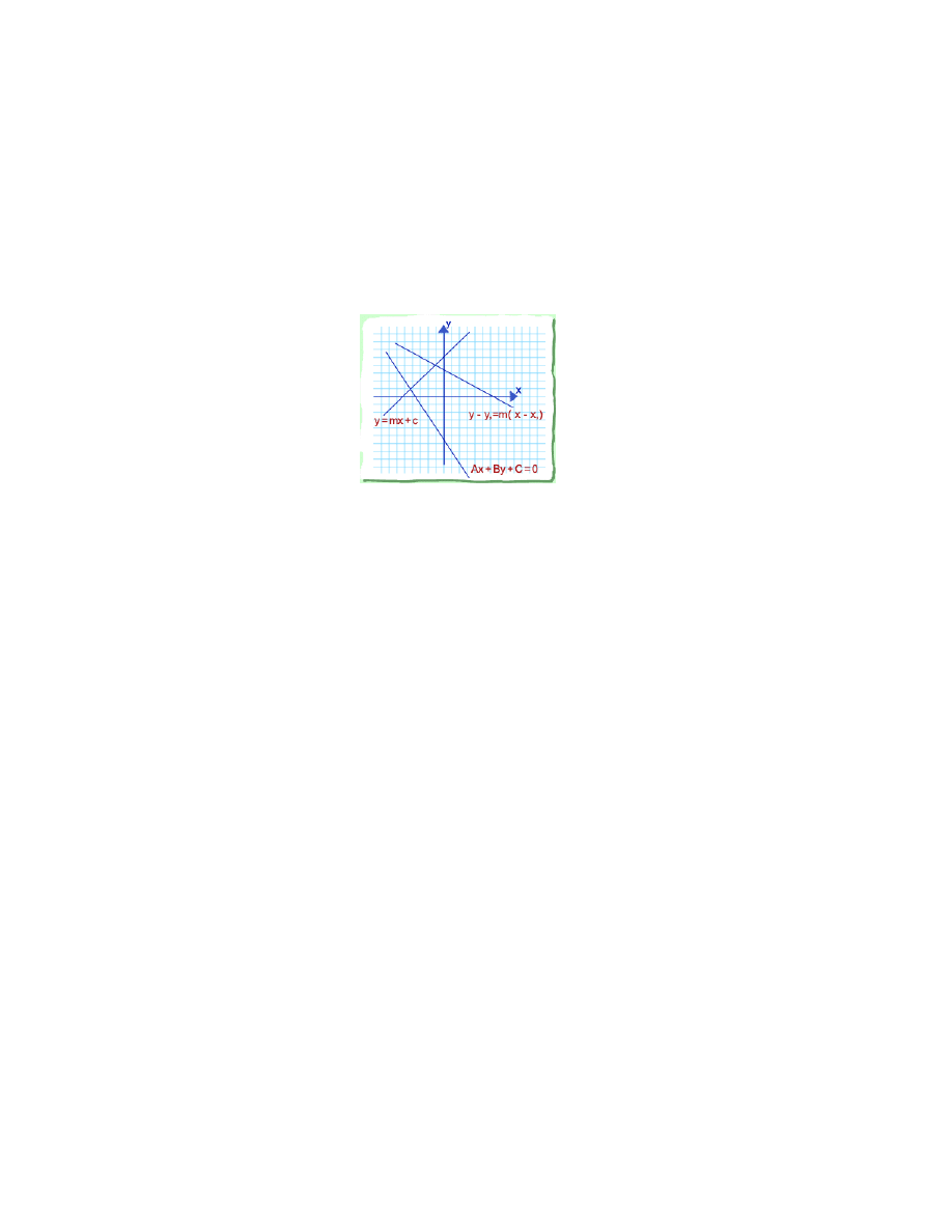
2. Let X be the set of straight lines in the plane:
Each such line has an equation Ax + By + C = 0 where if we multiply A, B, C by a
non-zero real number we get the same line. Let U
0
be the set of non-vertical lines.
For each line ` ∈ U
0
we have the equation
y = mx + c
where m, c are uniquely determined. So ϕ
0
(`) = (m, c) defines a coordinate chart
ϕ
0
: U
0
→ R
2
. Similarly if U
1
consists of the non-horizontal lines with equation
x = ˜
my + ˜
c
we have another chart ϕ
1
: U
1
→ R
2
.
Now U
0
∩ U
1
is the set of lines y = mx + c which are not horizontal, so m 6= 0. Thus
ϕ
0
(U
0
∩ U
1
) = {(m, c) ∈ R
2
: m 6= 0}
which is open. Moreover, y = mx + c implies x = m
−1
y − cm
−1
and so
ϕ
1
ϕ
−1
0
(m, c) = (m
−1
, −cm
−1
)
which is smooth with smooth inverse. Thus we have an atlas on the space of lines.
3. Consider R as an additive group, and the subgroup of integers Z ⊂ R. Let X be
the quotient group R/Z and p : R → R/Z the quotient homomorphism.
Set U
0
= p(0, 1) and U
1
= p(−1/2, 1/2). Since any two elements in the subset p
−1
(a)
differ by an integer, p restricted to (0, 1) or (−1/2, 1/2) is injective and so we have
coordinate charts
ϕ
0
= p
−1
: U
0
→ (0, 1),
ϕ
1
= p
−1
: U
1
→ (−1/2, 1/2).
5

Clearly U
0
and U
1
cover R/Z since the integer 0 ∈ U
1
.
We check:
ϕ
0
(U
0
∩ U
1
) = (0, 1/2) ∪ (1/2, 1),
ϕ
1
(U
0
∩ U
1
) = (−1/2, 0) ∪ (0, 1/2)
which are open sets. Finally, if x ∈ (0, 1/2), ϕ
1
ϕ
−1
0
(x) = x and if x ∈ (1/2, 1),
ϕ
1
ϕ
−1
0
(x) = x − 1. These maps are certainly smooth with smooth inverse so we have
an atlas on X = R/Z.
4. Let X be the extended complex plane X = C ∪ {∞}. Let U
0
= C with ϕ
0
(z) =
z ∈ C ∼
= R
2
. Now take
U
1
= C\{0} ∪ {∞}
and define ϕ
1
(˜
z) = ˜
z
−1
∈ C if ˜
z 6= ∞ and ϕ
1
(∞) = 0. Then
ϕ
0
(U
0
∩ U
1
) = C\{0}
which is open, and
ϕ
1
ϕ
−1
0
(z) = z
−1
=
x
x
2
+ y
2
− i
y
x
2
+ y
2
.
This is a smooth and invertible function of (x, y). We now have a 2-dimensional atlas
for X, the extended complex plane.
5.
Let X be n-dimensional real projective space, the set of 1-dimensional vector
subspaces of R
n+1
. Each subspace is spanned by a non-zero vector v, and we define
U
i
⊂ RP
n
to be the subset for which the i-th component of v ∈ R
n+1
is non-zero.
Clearly X is covered by U
1
, . . . , U
n+1
. In U
i
we can uniquely choose v such that the
ith component is 1, and then U
i
is in one-to-one correspondence with the hyperplane
x
i
= 1 in R
n+1
, which is a copy of R
n
. This is therefore a coordinate chart
ϕ
i
: U
i
→ R
n
.
The set ϕ
i
(U
i
∩ U
j
) is the subset for which x
j
6= 0 and is therefore open. Furthermore
ϕ
i
ϕ
−1
j
: {x ∈ R
n+1
: x
j
= 1, x
i
6= 0} → {x ∈ R
n+1
: x
i
= 1, x
j
6= 0}
is
v 7→
1
x
i
v
which is smooth with smooth inverse. We therefore have an atlas for RP
n
.
6

2.2
The definition of a manifold
All the examples above are actually manifolds, and the existence of an atlas is suf-
ficient to establish that, but there is a minor subtlety in the actual definition of a
manifold due to the fact that there are lots of choices of atlases. If we had used a
different basis for R
2
, our charts on the space X of straight lines would be different,
but we would like to think of X as an object independent of the choice of atlas. That’s
why we make the following definitions:
Definition 3 Two atlases {(U
α
, ϕ
α
)}, {(V
i
, ψ
i
)} are compatible if their union is an
atlas.
What this definition means is that all the extra maps ψ
i
ϕ
−1
α
must be smooth. Com-
patibility is clearly an equivalence relation, and we then say that:
Definition 4 A
differentiable structure
on X is an equivalence class of atlases.
Finally we come to the definition of a manifold:
Definition 5 An n-dimensional
differentiable manifold
is a space X with a differen-
tiable structure.
The upshot is this: to prove something is a manifold, all you need is to find one atlas.
The definition of a manifold takes into account the existence of many more atlases.
Many books give a slightly different definition – they start with a topological space,
and insist that the coordinate charts are homeomorphisms. This is fine if you see the
world as a hierarchy of more and more sophisticated structures but it suggests that
in order to prove something is a manifold you first have to define a topology. As we’ll
see now, the atlas does that for us.
First recall what a topological space is: a set X with a distinguished collection of
subsets V called open sets such that
1. ∅ and X are open
2. an arbitrary union of open sets is open
3. a finite intersection of open sets is open
7

Now suppose M is a manifold. We shall say that a subset V ⊆ M is open if, for each
α, ϕ
α
(V ∩ U
α
) is an open set in R
n
. One thing which is immediate is that V = U
β
is
open, from Definition 2.
We need to check that this gives a topology. Condition 1 holds because ϕ
α
(∅) = ∅
and ϕ
α
(M ∩ U
α
) = ϕ
α
(U
α
) which is open by Definition 1. For the other two, if V
i
is
a collection of open sets then because ϕ
α
is bijective
ϕ
α
((∪V
i
) ∩ U
α
) = ∪ϕ
α
(V
i
∩ U
α
)
ϕ
α
((∩V
i
) ∩ U
α
) = ∩ϕ
α
(V
i
∩ U
α
)
and then the right hand side is a union or intersection of open sets. Slightly less
obvious is the following:
Proposition 2.1 With the topology above ϕ
α
: U
α
→ ϕ
α
(U
α
) is a homeomorphism.
Proof: If V ⊆ U
α
is open then ϕ
α
(V ) = ϕ
α
(V ∩ U
α
) is open by the definition of the
topology, so ϕ
−1
α
is certainly continuous.
Now let W ⊂ ϕ
α
(U
α
) be open, then ϕ
−1
α
(W ) ⊆ U
α
and U
α
is open in M so we need
to prove that ϕ
−1
α
(W ) is open in M . But
ϕ
β
(ϕ
−1
α
(W ) ∩ U
β
) = ϕ
β
ϕ
−1
α
(W ∩ ϕ
α
(U
α
∩ U
β
))
(1)
From Definition 2 the set ϕ
α
(U
α
∩ U
β
) is open and hence its intersection with the
open set W is open. Now ϕ
β
ϕ
−1
α
is C
∞
with C
∞
inverse and so certainly a homeo-
morphism, and it follows that the right hand side of (1) is open. Thus the left hand
side ϕ
β
(ϕ
−1
α
W ∩ U
β
) is open and by the definition of the topology this means that
ϕ
−1
α
(W ) is open, i.e. ϕ
α
is continuous.
2
To make any reasonable further progress, we have to make two assumptions about
this topology which will hold for the rest of these notes:
• the manifold topology is Hausdorff
• in this topology we have a countable basis of open sets
Without these assumptions, manifolds are not even metric spaces, and there is not
much analysis that can reasonably be done on them.
8
2.3
Further examples of manifolds
We need better ways of recognizing manifolds than struggling to find explicit coordi-
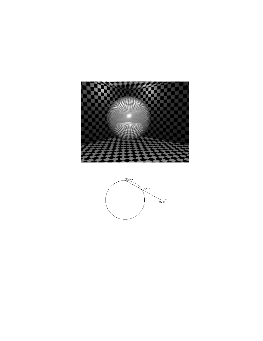
nate charts. For example, the sphere is a manifold
and although we can use stereographic projection to get an atlas:
there are other ways. Here is one.
Theorem 2.2 Let F : U → R
m
be a C
∞
function on an open set U ⊆ R
n+m
and
take c ∈ R
m
. Assume that for each a ∈ F
−1
(c), the derivative
DF
a
: R
n+m
→ R
m
is surjective. Then F
−1
(c) has the structure of an n-dimensional manifold which is
Hausdorff and has a countable basis of open sets.
Proof:
Recall that the derivative of F at a is the linear map DF
a
: R
n+m
→ R
m
such that
F (a + h) = F (a) + DF
a
(h) + R(a, h)
9
where R(a, h)/khk → 0 as h → 0.
If we write F (x
1
, . . . , x
n+m
) = (F
1
, . . . , F
m
) the derivative is the Jacobian matrix
∂F
i
∂x
j
(a)
1 ≤ i ≤ m, 1 ≤ j ≤ n + m
Now we are given that this is surjective, so the matrix has rank m. Therefore by
reordering the coordinates x
1
, . . . , x
n+m
we may assume that the square matrix
∂F
i
∂x
j
(a)
1 ≤ i ≤ m, 1 ≤ j ≤ m
is invertible.
Now define
G : U × R
m
→ R
n+m
by
G(x
1
, . . . , x
n+m
) = (F
1
, . . . , F
m
, x
m+1
, . . . , x
n+m
).
(2)
Then DG
a
is invertible.
We now apply the inverse function theorem to G, a proof of which is given in the
Appendix. It tells us that there is a neighbourhood V of x, and W of G(x) such
that G : V → W is invertible with smooth inverse. Moreover, the formula (2) shows
that G maps V ∩ F
−1
(c) to the intersection of W with the copy of R
n
given by
{x ∈ R
n+m
: x
i
= c
i
, 1 ≤ i ≤ m}. This is therefore a coordinate chart ϕ.
If we take two such charts ϕ
α
, ϕ
β
, then ϕ
α
ϕ
−1
β
is a map from an open set in {x ∈
R
n+m
: x
i
= c
1
, 1 ≤ i ≤ m} to another one which is the restriction of the map G
α
G
−1
β
of (an open set in) R
n+m
to itself. But this is an invertible C
∞
map and so we have
the requisite conditions for an atlas.
Finally, in the induced topology from R
n+m
, G
α
is a homeomorphism, so open sets
in the manifold topology are the same as open sets in the induced topology. Since
R
n+m
is Hausdorff with a countable basis of open sets, so is F
−1
(c).
2
We can now give further examples of manifolds:
Examples: 1. Let
S
n
= {x ∈ R
n+1
:
n+1
X
1
x
2
i
= 1}
10

be the unit n-sphere. Define F : R
n+1
→ R by
F (x) =
n+1
X
1
x
2
i
.
This is a C
∞
map and
DF
a
(h) = 2
X
i
a
i
h
i
is non-zero (and hence surjective in the 1-dimensional case) so long as a is not iden-
tically zero. If F (a) = 1, then
n+1
X
1
a
2
i
= 1 6= 0
so a 6= 0 and we can apply Theorem 2.2 and deduce that the sphere is a manifold.
2. Let O(n) be the space of n × n orthogonal matrices: AA
T
= 1. Take the vector
space M
n
of dimension n
2
of all real n × n matrices and define the function
F (A) = AA
T
to the vector space of symmetric n × n matrices. This has dimension n(n + 1)/2.
Then O(n) = F
−1
(I).
Differentiating F we have
DF
A
(H) = HA
T
+ AH
T
and putting H = KA this is
KAA
T
+ AA
T
K
T
= K + K
T
if AA
T
= I, i.e. if A ∈ F
−1
(I). But given any symmetric matrix S, taking K = S/2
shows that DF
I
is surjective and so, applying Theorem 2.2 we find that O(n) is a
manifold. Its dimension is
n
2
− n(n + 1)/2 = n(n − 1)/2.
2.4
Maps between manifolds
We need to know what a smooth map between manifolds is. Here is the definition:
11

Definition 6 A map F : M → N of manifolds is a
smooth map
if for each point
x ∈ M and chart (U
α
, ϕ
α
) in M with x ∈ U
α
and chart (V
i
, ψ
i
) of N with F (x) ∈ V
i
,
the composite function
ψ
i
F ϕ
−1
α
on F
−1
(V
i
) ∩ U
α
is a C
∞
function.
Note that it is enough to check that the above holds for one atlas – it will follow from
the fact that ϕ
α
ϕ
−1
β
is C
∞
that it then holds for all compatible atlases.
Exercise 2.3 Show that a smooth map is continuous in the manifold topology.
The natural notion of equivalence between manifolds is the following:
Definition 7 A
diffeomorphism
F : M → N is a smooth map with smooth inverse.
Example:
Take two of our examples above – the quotient group R/Z and the
1-sphere, the circle, S
1
. We shall show that these are diffeomorphic. First we define
a map
G : R/Z → S
1
by
G(x) = (cos 2πx, sin 2πx).
This is clearly a bijection. Take x ∈ U
0
⊂ R/Z then we can represent the point by
x ∈ (0, 1). Within the range (0, 1/2), sin 2πx 6= 0, so with F = x
2
1
+ x
2
2
, we have
∂F/∂x
2
6= 0. The use of the inverse function theorem in Theorem 2.2 then says that
x
1
is a local coordinate for S
1
, and in fact on the whole of (0, 1/2) cos 2πx is smooth
with smooth inverse. We proceed by taking the other similar open sets to check fully.
3
Tangent vectors and cotangent vectors
3.1
Existence of smooth functions
The most fundamental type of map between manifolds is a smooth map
f : M → R.
We can add these and multiply by constants so they form a vector space C
∞
(M ), the
space of C
∞
functions on M . In fact, under multiplication it is also a commutative
12

ring. So far, all we can assert is that the constant functions lie in this space, so let’s
see why there are lots and lots of global C
∞
functions. We shall use bump functions
and the Hausdorff property.
First note that the following function of one variable is C
∞
:
f (t) = e
−1/t
t > 0
= 0
t ≤ 0
Now form
g(t) =
f (t)
f (t) + f (1 − t)
so that g is identically 1 when t ≥ 1 and vanishes if t ≤ 0. Next write
h(t) = g(t + 2)g(2 − t).
This function is completely flat on top.
Finally make an n-dimensional version
k(x
1
, . . . , x
n
) = h(x
1
)h(x
2
) . . . h(x
n
).
We can rescale the domain of this so that it is zero outside some small ball of radius
2r and identically 1 inside the ball of radius r.
We shall use this construction several times later on. For the moment, let M be
any manifold and (U, ϕ
U
) a coordinate chart. Choose a function k of the type above
whose support (remember supp f = {x : f (x) 6= 0}) lies in ϕ
U
(U ) and define
f : M → R
by
f (x) = k ◦ ϕ
U
(x)
x ∈ U
= 0
x ∈ M \U.
13

Is this a smooth function? The answer is yes: clearly supp k is closed and bounded
in R
n
and so compact and since ϕ
U
is a homeomorphism, supp f is compact. If
y ∈ M \U then y is not in supp f , and if M is Hausdorff we can find an open set
containing y which does not intersect supp f . Then clearly f is smooth, since it is
zero in a neighbourhood of y.
3.2
The derivative of a function
Smooth functions exist in abundance. The question now is: we know what a differ-
entiable function is – so what is its derivative? We need to give some coordinate-
independent definition of derivative and this will involve some new concepts. The
derivative at a point a ∈ M will lie in a vector space T
∗
a
called the cotangent space.
First let’s address a simpler question – what does it mean for the derivative to vanish?
This is more obviously a coordinate-invariant notion because on a compact manifold
any function has a maximum, and in any coordinate system in a neighbourhood of
that point, its derivative must vanish. We can check that: if f : M → R is smooth
then
g = f ϕ
−1
α
is a C
∞
function of x
1
, . . . x
n
. Suppose its derivative vanishes at ϕ
U
(a) and now take
a different chart ϕ
β
with h = f ϕ
−1
β
. Then
g = f ϕ
−1
α
= f ϕ
−1
β
ϕ
β
ϕ
−1
α
= hϕ
β
ϕ
−1
α
.
But from the definition of an atlas, ϕ
β
ϕ
−1
α
is smooth with smooth inverse, so
g(x
1
, . . . , x
n
) = h(y
1
(x), . . . , y
n
(x))
and by the chain rule
∂g
∂x
i
=
X
j
∂h
∂y
j
(y(a))
∂y
j
∂x
i
(a).
Since y(x) is invertible, its Jacobian matrix is invertible, so that Dg
a
= 0 if and
only if Dh
y(a)
= 0. We have checked then that the vanishing of the derivative at a
point a is independent of the coordinate chart. We let Z
a
⊂ C
∞
(M ) be the subset of
functions whose derivative vanishes at a. Since Df
a
is linear in f the subset Z
a
is a
vector subspace.
Definition 8 The
cotangent space
T
∗
a
at a ∈ M is the quotient space
T
∗
a
= C
∞
(M )/Z
a
.
The derivative of a function f at a is its image in this space and is denoted (df )
a
.
14

Here we have simply defined the derivative as all functions modulo those whose deriva-
tive vanishes. It’s almost a tautology, so to get anywhere we have to prove something
about T
∗
a
. First note that if ψ is a smooth function on a neighbourhood of x, we
can multiply it by a bump function to extend it to M and then look at its image in
T
∗
a
= C
∞
(M )/Z
a
. But its derivative in a coordinate chart around a is independent of
the bump function, because all such functions are identically 1 in a neighbourhood
of a. Hence we can actually define the derivative at a of smooth functions which
are only defined in a neighbourhood of a. In particular we could take the coordinate
functions x
1
, . . . , x
n
. We then have
Proposition 3.1 Let M be an n-dimensional manifold, then
• the cotangent space T
∗
a
at a ∈ M is an n-dimensional vector space
• if (U, ϕ) is a coordinate chart around x with coordinates x
1
, . . . , x
n
, then the
elements (dx
1
)
a
, . . . (dx
n
)
a
form a basis for T
∗
a
• if f ∈ C
∞
(M ) and in the coordinate chart, f ϕ
−1
= φ(x
1
, . . . , x
n
) then
(df )
a
=
X
i
∂φ
∂x
i
(ϕ(a))(dx
i
)
a
(3)
Proof: If f ∈ C
∞
(M ), with f ϕ
−1
= φ(x
1
, . . . , x
n
) then
f −
X
∂φ
∂x
i
(ϕ(a))x
i
is a (locally defined) smooth function whose derivative vanishes at a, so
(df )
a
=
X
∂f
∂x
i
(ϕ(a))(dx
i
)
a
and (dx
1
)
a
, . . . (dx
n
)
a
span T
∗
a
.
If
P
i
λ
i
(dx
i
)
a
= 0 then
P
i
λ
i
x
i
has vanishing derivative at a and so λ
i
= 0 for all i.
2
Remark:
It is rather heavy handed to give two symbols f, φ for a function and its
representation in a given coordinate system, so often in what follows we shall use just
f . Then we can write (3) as
df =
X
∂f
∂x
i
dx
i
.
15
With a change of coordinates (x
1
, . . . , x
n
) → (y
1
(x), . . . , y
n
(x)) the formalism gives
df =
X
j
∂f
∂y
j
dy
j
=
X
i,j
∂f
∂y
j
∂y
j
∂x
i
dx
i
.
Definition 9 The
tangent space
T
a
at a ∈ M is the dual space of the cotangent space
T
∗
a
.
This is a roundabout way of defining T
a
, but since the double dual V
∗
∗ of a finite
dimensional vector space is naturally isomorphic to V the notation is consistent. If
x
1
, . . . , x
n
is a local coordinate system at a and (dx
1
)
a
, . . . , (dx
n
)
a
the basis of T
∗
a
defined in (3.1) then the dual basis for the tangent space T
a
is denoted
∂
∂x
1
a
, . . . ,
∂
∂x
1
a
.
This definition at first sight seems far away from our intuition about the tangent
space to a surface in R
3
:
The problem arises because our manifold M does not necessarily sit in Euclidean
space and we have to define a tangent space intrinsically. The link is provided by the
notion of directional derivative. If f is a function on a surface in R
3
, then for every
tangent direction u at a we can define the derivative of f at a in the direction u,
which is a real number: u · ∇f (a) or DF
a
(u). Imitating this gives the following:
Definition 10 A
tangent vector
at a point a ∈ M is a linear map X
a
: C
∞
(M ) → R
such that
X
a
(f g) = f (a)X
a
g + g(a)X
a
f.
This is the formal version of the Leibnitz rule for differentiating a product.
16

Now if ξ ∈ T
a
it lies in the dual space of T
∗
a
= C
∞
(M )/Z
a
and so
f 7→ ξ((df )
a
)
is a linear map from C
∞
(M ) to R. Moreover from (3),
d(f g)
a
= f (a)(dg)
a
+ g(a)(df )
a
and so
X
a
(f ) = ξ((df )
a
)
is a tangent vector at a. In fact, any tangent vector is of this form, but the price paid
for the nice algebraic definition in (10) which is the usual one in textbooks is that we
need a lemma to prove it.
Lemma 3.2 Let X
a
be a tangent vector at a and f a smooth function whose derivative
at a vanishes. Then X
a
f = 0.
Proof: Use a coordinate system near a. By the fundamental theorem of calculus,
f (x) − f (a) =
Z
1
0
∂
∂t
f (a + t(x − a))dt
=
X
i
(x
i
− a
i
)
Z
1
0
∂f
∂x
i
(a + t(x − a))dt.
If (df )
a
= 0 then
g
i
(x) =
Z
1
0
∂f
∂x
i
(a + t(x − a))dt
vanishes at x = a, as does x
i
− a
i
. Now although these functions are defined locally,
using a bump function we can extend them to M , so that
f = f (a) +
X
i
g
i
h
i
(4)
where g
i
(a) = h
i
(a) = 0.
By the Leibnitz rule
X
a
(1) = X
a
(1.1) = 2X
a
(1)
which shows that X
a
annihilates constant functions. Applying the rule to (4)
X
a
(f ) = X
a
(
X
i
g
i
h
i
) =
X
i
(g
i
(a)X
a
h
i
+ h
i
(a)X
a
g
i
) = 0.
This means that X
a
: C
∞
(M ) → R annihilates Z
a
and is well defined on T
∗
a
=
C
∞
(M )/Z
a
and so X
a
∈ T
a
.
2
17
The vectors in the tangent space are therefore the tangent vectors as defined by (10).
Locally, in coordinates, we can write
X
a
=
n
X
i
c
i
∂
∂x
i
a
and then
X
a
(f ) =
X
i
c
i
∂f
∂x
i
(a)
(5)
3.3
Derivatives of smooth maps
Suppose F : M → N is a smooth map and f ∈ C
∞
(N ). Then f ◦ F is a smooth
function on M .
Definition 11 The
derivative
at a ∈ M of the smooth map F : M → N is the
homomorphism of tangent spaces
DF
a
: T
a
M → T
F (a)
N
defined by
DF
a
(X
a
)(f ) = X
a
(f ◦ F ).
This is an abstract, coordinate-free definition. Concretely, we can use (5) to see that
DF
a
∂
∂x
i
a
(f ) =
∂
∂x
i
(f ◦ F )(a)
=
X
j
∂F
j
∂x
i
(a)
∂f
∂y
j
(F (a)) =
X
j
∂F
j
∂x
i
(a)
∂
∂y
j
F (a)
f
Thus the derivative of F is an invariant way of defining the Jacobian matrix.
With this definition we can give a generalization of Theorem 2.2 – the proof is virtually
the same and is omitted.
Theorem 3.3 Let F : M → N be a smooth map and c ∈ N be such that at each
point a ∈ F
−1
(c) the derivative DF
a
is surjective. Then F
−1
(c) is a smooth manifold
of dimension dim M − dim N .
18

In the course of the proof, it is easy to see that the manifold structure on F
−1
(c)
makes the inclusion
ι : F
−1
(c) ⊂ M
a smooth map, whose derivative is injective and maps isomorphically to the kernel of
DF . So when we construct a manifold like this, its tangent space at a is
T
a
∼
= Ker DF
a
.
This helps to understand tangent spaces for the case where F is defined on R
n
:
Examples:
1. The sphere S
n
is F
−1
(1) where F : R
n+1
→ R is given by
F (x) =
X
i
x
2
i
.
So here
DF
a
(x) = 2
X
i
x
i
a
i
and the kernel of DF
a
consists of the vectors orthogonal to a, which is our usual
vision of the tangent space to a sphere.
2. The orthogonal matrices O(n) are given by F
−1
(I) where F (A) = AA
T
. At A = I,
the derivative is
DF
I
(H) = H + H
T
so the tangent space to O(n) at the identity matrix is Ker DF
I
, the space of skew-
symmetric matrices H = −H
T
.
The examples above are of manifolds F
−1
(c) sitting inside M and are examples of
submanifolds. Here we shall adopt the following definition of a submanifold, which is
often called an embedded submanifold:
Definition 12 A manifold M is a
submanifold
of N if there is an inclusion map
ι : M → N
such that
• ι is smooth
19
• Dι
x
is injective for each x ∈ M
• the manifold topology of M is the induced topology from N
Remark: The topological assumption avoids a situation like this:
ι(t) = (t
2
− 1, t(t
2
− 1)) ∈ R
2
for t ∈ (−1, 1). This is smooth, injective with injective derivative, but any open set
in R
2
containing 0 intersects both ends of the interval. The curve is the left hand
loop of the singular cubic: y
2
= x
2
(x + 1).
4
Vector fields
4.1
The tangent bundle
Think of the wind velocity at each point of the earth.
20
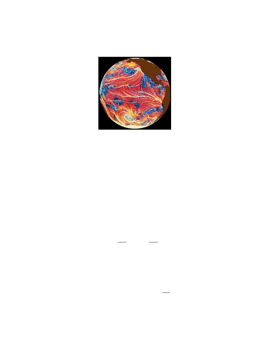
This is an example of a vector field on the 2-sphere S
2
. Since the sphere sits inside
R
3
, this is just a smooth map X : S
2
→ R
3
such that X(x) is tangential to the sphere
at x.
Our problem now is to define a vector field intrinsically on a general manifold M ,
without reference to any ambient space. We know what a tangent vector at a ∈ M
is – a vector in T
a
– but we want to describe a smoothly varying family of these. To
do this we need to fit together all the tangent spaces as a ranges over M into a single
manifold called the tangent bundle. We have n degrees of freedom for a ∈ M and n
for each tangent space T
a
so we expect to have a 2n-dimensional manifold. So the set
to consider is
T M =
[
x∈M
T
x
the disjoint union of all the tangent spaces.
First let (U, ϕ
U
) be a coordinate chart for M . Then for x ∈ U the tangent vectors
∂
∂x
1
x
, . . . ,
∂
∂x
n
x
provide a basis for each T
x
. So we have a bijection
ψ
U
: U × R
n
→
[
x∈U
T
x
defined by
ψ
U
(x, y
1
, . . . , y
n
) =
n
X
1
y
i
∂
∂x
i
x
.
Thus
Φ
U
= (ϕ
U
, id) ◦ ψ
−1
:
[
x∈U
T
x
→ ϕ
U
(U ) × R
n
21
is a coordinate chart for
V =
[
x∈U
T
x
.
Given U
α
, U
β
coordinate charts on M , clearly
Φ
α
(V
α
∩ V
β
) = ϕ
α
(U
α
∩ U
β
) × R
n
which is open in R
2n
. Also, if (x
1
, . . . , x
n
) are coordinates on U
α
and (˜
x
1
, . . . , ˜
x
n
) on
U
β
then
∂
∂x
i
x
=
X
j
∂ ˜
x
j
∂x
i
∂
∂ ˜
x
j
x
the dual of (3). It follows that
Φ
β
Φ
−1
α
(x
1
, . . . , x
n
, y
1
. . . , y
n
) = (˜
x
1
, . . . , ˜
x
n
,
X
j
∂ ˜
x
1
∂x
i
y
i
, . . . ,
X
i
∂ ˜
x
n
∂x
i
y
i
).
and since the Jacobian matrix is smooth in x, linear in y and invertible, Φ
β
Φ
−1
α
is
smooth with smooth inverse and so (V
α
, Φ
α
) defines an atlas on T M .
Definition 13 The
tangent bundle
of a manifold M is the 2n-dimensional differen-
tiable structure on T M defined by the above atlas.
The construction brings out a number of properties. First of all the projection map
p : T M → M
which assigns to X
a
∈ T
a
M the point a is smooth with surjective derivative, because
in our local coordinates it is defined by
p(x
1
, . . . , x
n
, y
1
, . . . , y
n
) = (x
1
, . . . , x
n
).
The inverse image p
−1
(a) is the vector space T
a
and is called a fibre of the projection.
Finally, T M is Hausdorff because if X
a
, X
b
lie in different fibres, since M is Hausdorff
we can separate a, b ∈ M by open sets U, U
0
and then the open sets p
−1
(U ), p
−1
(U
0
)
separate X
a
, X
b
in T M . If X
a
, Y
a
are in the same tangent space then they lie in a
coordinate neighbourhood which is homeomorphic to an open set of R
2n
and so can
be separated there. Since M has a countable basis of open sets and R
n
does, it is
easy to see that T M also has a countable basis.
We can now define a vector field:
22
Definition 14 A
vector field
on a manifold is a smooth map
X : M → T M
such that
p ◦ X = id
M
.
This is a clear global definition. What does it mean? We just have to spell things
out in local coordinates. Since p ◦ X = id
M
,
X(x
1
, . . . , x
n
) = (x
1
, . . . , x
n
, y
1
(x), . . . , y
n
(x))
where y
i
(x) are smooth functions. Thus the tangent vector X(x) is given by
X(x) =
X
i
y
i
(x)
∂
∂x
i
x
which is a smoothly varying field of tangent vectors.
Remark:
We shall meet other manifolds Q with projections p : Q → M and the
general terminology is that a smooth map s : M → Q for which p ◦ s = id
M
is called a
section. When Q = T M is the tangent bundle we always have the zero section given
by the vector field X = 0. Using a bump function ψ we can easily construct other
vector fields by taking a coordinate system, writing
X(x) =
X
i
y
i
(x)
∂
∂x
i
x
multiplying by ψ and extending.
Remark:
Clearly we can do a similar construction using the cotangent spaces T
∗
a
instead of the tangent spaces T
a
, and using the basis
(dx
1
)
x
, . . . , (dx
n
)
x
instead of the dual basis
∂
∂x
1
x
, . . . ,
∂
∂x
1
x
.
This way we form the cotangent bundle T
∗
M . The derivative of a function f is then
a map df : M → T M satisfying p ◦ df = id
M
, though not every such map of this
form is a derivative. The tangent bundle and cotangent bundle are examples of vector
bundles.
23

Perhaps we should say here that the tangent bundle and cotangent bundle are exam-
ples of vector bundles. Here is the general definition:
Definition 15 A real
vector bundle
of rank m on a manifold M is a manifold E with
a smooth projection p : E → M such that
• each fibre p
−1
(x) has the structure of an m-dimensional real vector space
• each point x ∈ M has a neighbourhood U and a diffeomorphism
ψ
U
: p
−1
(U ) ∼
= U × R
m
such that ψ
U
maps the vector space p
−1
(x) isomorphically to the vector space
{x} × R
m
• on the intersection U ∩ V
ψ
−1
U
ψ
V
: U ∩ V × R
m
→ U ∩ V × R
m
is of the form
(x, v) 7→ (x, g
U V
(x)v)
where g
U V
(x) is a smooth function on U ∩V with values in the space of invertible
m × m matrices.
For the tangent and cotangent bundle, g
U V
is the Jacobian matrix of a change of
coordinates or its inverse transpose.
4.2
Vector fields as derivations
The algebraic definition of tangent vector in Definition 10 shows that a vector field
X maps a C
∞
function to a function on M :
X(f )(x) = X
x
(f )
and the local expression for X means that
X(f )(x) =
X
i
y
i
(x)
∂
∂x
i
x
(f ) =
X
i
y
i
(x)
∂f
∂x
i
(x).
Since the y
i
(x) are smooth, X(f ) is again smooth and satisfies the Leibnitz property
X(f g) = f (Xg) + g(Xf ).
In fact, any linear transformation with this property (called a derivation of the algebra
C
∞
(M )) is a vector field:
24

Proposition 4.1 Let X : C
∞
(M ) → C
∞
(M ) be a linear map which satisfies
X(f g) = f (Xg) + g(Xf ).
Then X is a vector field.
Proof:
For each a ∈ M , X
a
(f ) = X(f )(a) satisfies the conditions for a tangent
vector at a, so X defines a map X : M → T M with p ◦ X = id
M
, and so locally can
be written as
X
x
=
X
i
y
i
(x)
∂
∂x
i
x
.
We just need to check that the y
i
(x) are smooth, and for this it suffices to apply
X to a coordinate function x
i
extended by using a bump function in a coordinate
neighbourhood. We get
Xx
i
= y
i
(x)
and since by assumption X maps smooth functions to smooth functions, this is
smooth.
2
The characterization of vector fields given by Proposition 4.1 immediately leads to a
way of combining two vector fields X, Y to get another. Consider both X and Y as
linear maps from C
∞
(M ) to itself and compose them. Then
XY (f g) = X(f (Y g) + g(Y f )) = (Xf )(Y g) + f (XY g) + (Xg)(Y f ) + g(XY f )
Y X(f g) = Y (f (Xg) + g(Xf )) = (Y f )(Xg) + f (Y Xg) + (Y g)(Xf ) + g(Y Xf )
and subtracting and writing [X, Y ] = XY − Y X we have
[X, Y ](f g) = f ([X, Y ]g) + g([X, Y ]f )
which from Proposition 4.1 means that [X, Y ] is a vector field.
Definition 16 The
Lie bracket
of two vector fields X, Y is the vector field [X, Y ].
Example: If M = R then X = f d/dx, Y = gd/dx and so
[X, Y ] = (f g
0
− gf
0
)
d
dx
.
We shall later see that there is a geometrical origin for the Lie derivative.
25

4.3
One-parameter groups of diffeomorphisms
Think of wind velocity (assuming it is constant in time) on the surface of the earth
as a vector field on the sphere S
2
. There is another interpretation we can make. A
particle at position x ∈ S
2
moves after time t seconds to a position ϕ
t
(x) ∈ S
2
. After
a further s seconds it is at
ϕ
t+s
(x) = ϕ
s
(ϕ
t
(x)).
What we get this way is a homomorphism of groups: from the additive group R to
the group of diffeomorphisms of S
2
under the operation of composition. The technical
definition is the following:
Definition 17 A
one-parameter group of diffeomorphisms
of a manifold M is a
smooth map
ϕ : M × R → M
such that (writing ϕ
t
(x) = ϕ(x, t))
• ϕ
t
: M → M is a diffeomorphism
• ϕ
0
= id
• ϕ
s+t
= ϕ
s
◦ ϕ
t
.
We shall show that vector fields generate one-parameter groups of diffeomorphisms,
but only under certain hypotheses. If instead of the whole surface of the earth our
manifold is just the interior of the UK and the wind is blowing East-West, clearly after
however short a time, some particles will be blown offshore, so we cannot hope for
ϕ
t
(x) that works for all x and t. The fact that the earth is compact is one reason why it
works there, and this is one of the results below. The idea, nevertheless, works locally
and is a useful way of understanding vector fields as “infinitesimal diffeomorphisms”
rather than as abstract derivations of functions.
To make the link with vector fields, suppose ϕ
t
is a one-parameter group of diffeo-
morphisms and f a smooth function. Then
f (ϕ
t
(a))
is a smooth function of t and we write
∂
∂t
f (ϕ
t
(a))|
t=0
= X
a
(f ).
26

It is straightforward to see that, since ϕ
0
(a) = a the Leibnitz rule holds and this is a
tangent vector at a, and so as a = x varies we have a vector field. In local coordinates
we have
ϕ
t
(x
1
, . . . , x
n
) = (y
1
(x, t), . . . , y
n
(x, t))
and
∂
∂t
f (y
1
, . . . , y
n
) =
X
i
∂f
∂y
i
(y)
∂y
i
∂t
(x)|
t=0
=
X
i
c
i
(x)
∂f
∂x
i
(x)
which yields the vector field
X =
X
i
c
i
(x)
∂
∂x
i
.
We now want to reverse this: go from the vector field to the diffeomorphism. The
first point is to track that “trajectory” of a single particle.
Definition 18 An
integral curve
of a vector field X is a smooth map ϕ : (α, β) ⊂
R → M such that
Dϕ
t
d
dt
= X
ϕ(t)
.
Example: Suppose M = R
2
with coordinates (x, y) and X = ∂/∂x. The derivative
Dϕ of the smooth function ϕ(t) = (x(t), y(t)) is
Dϕ
d
dt
=
dx
dt
∂
∂x
+
dy
dt
∂
∂y
so the equation for an integral curve of X is
dx
dt
= 1
dy
dt
= 0
which gives
ϕ(t) = (t + a
1
, a
2
).
In our wind analogy, the particle at (a
1
, a
2
) is transported to (t + a
1
, a
2
).
27

In general we have:
Theorem 4.2 Given a vector field X on a manifold M and a ∈ M there exists a
maximal integral curve of X through a.
By “maximal” we mean that the interval (α, β) is maximal – as we saw above it may
not be the whole of the real numbers.
Proof: First consider a coordinate chart (U
α
, ϕ
α
) around a then if
X =
X
i
c
i
(x)
∂
∂x
i
the equation
Dϕ
t
d
dt
= X
ϕ(t)
can be written as the system of ordinary differential equations
dx
i
dt
= c
i
(x
1
, . . . , x
n
).
The existence and uniqueness theorem for ODE’s (see Appendix) asserts that there
is some interval on which there is a unique solution with initial condition
(x
1
(0), . . . , x
n
(0)) = ϕ
α
(a).
Suppose ϕ : (α, β) → M is any integral curve with ϕ(0) = a. For each x ∈ (α, β)
the subset ϕ([0, x]) ⊂ M is compact, so it can be covered by a finite number of
coordinate charts, in each of which we can apply the existence and uniqueness theorem
to intervals [0, α
1
], [α
1
, α
2
], . . . , [α
n
, x]. Uniqueness implies that these local solutions
agree with ϕ on any subinterval containing 0.
We then take the maximal open interval on which we can define ϕ.
2
To find the one-parameter group of diffeomorphisms we now let a ∈ M vary. In the
example above, the integral curve through (a
1
, a
2
) was t 7→ (t+a
1
, a
2
) and this defines
the group of diffeomorphisms
ϕ
t
(x
1
, x
2
) = (t + x
1
, x
2
).
Theorem 4.3 Let X be a vector field on a manifold M and for (t, x) ∈ R × M , let
ϕ
(
x, t) = ϕ
t
(x) be the maximal integral curve of X through x. Then
28

• the map (t, x) 7→ ϕ
t
(x) is smooth
• ϕ
t
◦ ϕ
s
= ϕ
t+s
wherever the maps are defined
• if M is compact, then ϕ
t
(x) is defined on R × M and gives a one-parameter
group of diffeomorphisms.
Proof: The previous theorem tells us that for each a ∈ M we have an open interval
(α(a), β(a)) on which the maximal integral curve is defined. The local existence
theorem also gives us that there is a solution for initial conditions in a neighbourhood
of a so the set
{(t, x) ∈ R × M : t ∈ (α(x), β(x))}
is open. This is the set on which ϕ
t
(x) is maximally defined.
The theorem (see Appendix) on smooth dependence on initial conditions tells us that
(t, x) 7→ ϕ
t
(x) is smooth.
Consider ϕ
t
◦ ϕ
s
(x). If we fix s and vary t, then this is the unique integral curve of X
through ϕ
s
(x). But ϕ
t+s
(x) is an integral curve which at t = 0 passes through ϕ
s
(x).
By uniqueness they must agree so that ϕ
t
◦ ϕ
s
= ϕ
t+s
. (Note that ϕ
t
◦ ϕ
−t
= id shows
that we have a diffeomorphism wherever it is defined).
Now consider the case where M is compact. For each x ∈ M , we have an open
interval (α(x), β(x)) containing 0 and an open set U
x
⊆ M on which ϕ
t
(x) is defined.
Cover M by {U
x
}
x∈M
and take a finite subcovering U
x
1
, . . . , U
x
N
, and set
I =
N
\
1
(α(x
i
), β(x
i
))
which is an open interval containing 0. By construction, for t ∈ I we get
ϕ
t
: I × M → M
which defines an integral curve (though not necessarily maximal) through each point
x ∈ M and with ϕ
0
(x) = x. We need to extend to all real values of t.
If s, t ∈ R, choose n such that (|s| + |t|)/n ∈ I and define (where multiplication is
composition)
ϕ
t
= (ϕ
t/n
)
n
,
ϕ
s
= (ϕ
s/n
)
n
.
Now because t/n, s/n and (s + t)/n lie in I we have
ϕ
t/n
ϕ
s/n
= ϕ
(s+t)/n
= ϕ
s/n
ϕ
t/n
29

and so because ϕ
t/n
and ϕ
s/n
commute, we also have
ϕ
t
ϕ
s
= (ϕ
t/n
)
n
(ϕ
s/n
)
n
= (ϕ
(s+t)/n
)
n
= ϕ
s+t
which completes the proof.
2
4.4
The Lie bracket revisited
All the objects we shall consider will have the property that they can be transformed
naturally by a diffeomorphism, and the link between vector fields and diffeomorphisms
we have just observed provides an “infinitesimal’ version of this.
Given a diffeomorphism F : M → M and a smooth function f we get the transformed
function f ◦ F . When F = ϕ
t
, generated according to the theorems above by a vector
field X, we then saw that
∂
∂t
f (ϕ
t
)|
t=0
= X(f ).
So: the natural action of diffeomorphisms on functions specializes through one-parameter
groups to the derivation of a function by a vector field.
Now suppose Y is a vector field, considered as a map Y : M → T M . With a
diffeomorphism F : M → M , its derivative DF
x
: T
x
→ T
F (x)
gives
DF
x
(Y
x
) ∈ T
F (x)
.
This defines a new vector field ˜
Y by
˜
Y
F (x)
= DF
x
(Y
x
)
(6)
Thus for a function f ,
( ˜
Y )(f ◦ F ) = (Y f ) ◦ F
(7)
Now if F = ϕ
t
for a one-parameter group, we have ˜
Y
t
and we can differentiate to get
˙
Y =
∂
∂t
˜
Y
t
t=0
From (7) this gives
˙
Y f + Y (Xf ) = XY f
so that ˙
Y = XY − Y X is the Lie derivative defined above. Thus the natural action of
diffeomorphisms on vector fields specializes through one-parameter groups to the Lie
bracket [X, Y ].
30

5
Tensor products
We have so far encountered vector fields and the derivatives of smooth functions as
analytical objects on manifolds. These are examples of a general class of objects
called tensors which we shall encounter in more generality. The starting point is pure
linear algebra.
Let V, W be two finite-dimensional vector spaces over R. We are going to define a
new vector space V ⊗ W with two properties:
• if v ∈ V and w ∈ W then there is a product v ⊗ w ∈ V ⊗ W
• the product is bilinear:
(λv
1
+ µv
2
) ⊗ w = λv
1
⊗ w + µv
2
⊗ w
v ⊗ (λw
1
+ µw
2
) = λv ⊗ w
1
+ µv ⊗ w
2
In fact, it is the properties of the vector space V ⊗ W which are more important
than what it is (and after all what is a real number? Do we always think of it as an
equivalence class of Cauchy sequences of rationals?).
Proposition 5.1 The tensor product V ⊗ W has the universal property that if B :
V × W → U is a bilinear map to a vector space U then there is a unique linear map
β : V ⊗ W → U
such that B(v, w) = β(v ⊗ w).
There are various ways to define V ⊗ W . In the finite-dimensional case we can say
that V ⊗ W is the dual space of the space of bilinear forms on V × W : i.e. maps
B : V × W → R such that
B(λv
1
+ µv
2
, w) = λB(v
1
, w) + µB(v
2
, w)
B(v, λw
1
+ µw
2
) = λB(v, w
1
) + µB(v, w
2
)
Given v, w ∈ V, W we then define v ⊗ w ∈ V ⊗ W as the map
(v ⊗ w)(B) = B(v, w).
This satisfies the universal property because given B : V × W → U and ξ ∈ U
∗
, ξ ◦ B
is a bilinear form on V × W and defines a linear map from U
∗
to the space of bilinear
forms. The dual map is the required homomorphism β from V ⊗ W to (U
∗
)
∗
= U .
31

A bilinear form B is uniquely determined by its values B(v
i
, w
j
) on basis vectors
v
1
, . . . , v
m
for V and w
1
, . . . w
n
for W which means the dimension of the vector space
of bilinear forms is mn, as is its dual space V ⊗ W . In fact, we can easily see that
the mn vectors
v
i
⊗ w
j
form a basis for V ⊗ W . It is important to remember though that a typical element
of V ⊗ W can only be written as a sum
X
i,j
a
ij
v
i
⊗ w
j
and not as a pure product v ⊗ w.
Taking W = V we can form multiple tensor products
V ⊗ V,
V ⊗ V ⊗ V = ⊗
3
V,
. . .
We can think of ⊗
p
V as the dual space of the space of p-fold multilinear forms on V .
Mixing degrees we can even form the tensor algebra:
T (V ) = ⊕
∞
k=0
(⊗
k
V ).
An element of T (V ) is a finite sum
λ1 + v
0
+
X
v
i
⊗ v
j
+ . . . +
X
v
i
1
⊗ v
i
2
. . . ⊗ v
i
p
of products of vectors v
i
∈ V . The obvious multiplication process is based on extend-
ing by linearity the product
(v
1
⊗ . . . ⊗ v
p
)(u
1
⊗ . . . ⊗ u
q
) = v
1
⊗ . . . ⊗ v
p
⊗ u
1
⊗ . . . ⊗ u
q
It is associative, but noncommutative.
For the most part we shall be interested in only a quotient of this algebra, called the
exterior algebra. A down-to-earth treatment of this is in the Section b3 Projective
Geometry Notes on the Mathematical Institute website.
5.1
The exterior algebra
Let T (V ) be the tensor algebra of a real vector space V and let I(V ) be the ideal
generated by elements of the form
v ⊗ v
where v ∈ V . So I(V ) consists of all sums of multiples by T (V ) on the left and right
of these generators.
32

Definition 19 The
exterior algebra
of V is the quotient
Λ
∗
V = T (V )/I(V ).
If π : T (V ) → Λ
∗
V is the quotient projection then we set
Λ
p
V = π(⊗
p
V )
and call this the p-fold exterior power of V . We can think of this as the dual space of
the space of multilinear forms M (v
1
, . . . , v
p
) on V which vanish if any two arguments
coincide – the so-called alternating multilinear forms. If a ∈ ⊗
p
V, b ∈ ⊗
q
V then
a ⊗ b ∈ ⊗
p+q
V and taking the quotient we get a product called the exterior product:
Definition 20 The
exterior product
of α = π(a) ∈ Λ
p
V and β = π(b) ∈ Λ
q
V is
α ∧ β = π(a ⊗ b).
Remark: As in the Projective Geometry Notes, if v
1
, . . . , v
p
∈ V then we define an
element of the dual space of the space of alternating multilinear forms by
v
1
∧ v
2
∧ . . . ∧ v
p
(M ) = M (v
1
, . . . , v
p
).
The key properties of the exterior algebra follow:
Proposition 5.2 If α ∈ Λ
p
V, β ∈ Λ
q
V then
α ∧ β = (−1)
pq
β ∧ α.
Proof: Because for v ∈ V , v ⊗ v ∈ I(V ), it follows that v ∧ v = 0 and hence
0 = (v
1
+ v
2
) ∧ (v
1
+ v
2
) = 0 + v
1
∧ v
2
+ v
2
∧ v
1
+ 0.
So interchanging any two entries from V in an expression like
v
1
∧ . . . ∧ v
k
changes the sign.
Write α as a linear combination of terms v
1
∧ . . . ∧ v
p
and β as a linear combination
of w
1
∧ . . . ∧ w
q
and then, applying this rule to bring w
1
to the front we see that
(v
1
∧ . . . ∧ v
p
) ∧ (w
1
∧ . . . ∧ w
q
) = (−1)
p
w
1
∧ v
1
∧ . . . v
p
∧ w
2
∧ . . . ∧ w
q
.
For each of the q w
i
’s we get another factor (−1)
p
so that in the end
(w
1
∧ . . . ∧ w
q
)(v
1
∧ . . . ∧ v
p
) = (−1)
pq
(v
1
∧ . . . ∧ v
p
)(w
1
∧ . . . ∧ w
q
).
2
33

Proposition 5.3 If dim V = n then dim Λ
n
V = 1.
Proof:
Let w
1
, . . . , w
n
be n vectors on V and relative to some basis let M be the
square matrix whose columns are w
1
, . . . , w
n
. then
B(w
1
, . . . , w
n
) = det M
is a non-zero n-fold multilinear form on V . Moreover, if any two of the w
i
coincide,
the determinant is zero, so this is a non-zero alternating n-linear form – an element
in the dual space of Λ
n
V .
On the other hand, choose a basis v
1
, . . . , v
n
for V , then anything in ⊗
n
V is a linear
combination of terms like v
i
1
⊗ . . . ⊗ v
i
n
and so anything in Λ
n
V is, after using
Proposition 5.2 a linear combination of v
1
∧ . . . ∧ v
n
.
Thus Λ
n
V is non-zero and at most one-dimensional hence is one-dimensional.
2
Proposition 5.4 let v
1
, . . . , v
n
be a basis for V , then the
n
p
elements v
i
1
∧v
i
2
∧. . .∧v
i
p
for i
1
< i
2
< . . . < i
p
form a basis for Λ
p
V .
Proof: By reordering and changing the sign we can get any exterior product of the
v
i
’s so these elements clearly span Λ
p
V . Suppose then that
X
a
i
1
...i
p
v
i
1
∧ v
i
2
∧ . . . ∧ v
i
p
= 0.
Because i
1
< i
2
< . . . < i
p
, each term is uniquely indexed by the subset {i
1
, i
2
, . . . , i
p
} =
I ⊆ {1, 2, . . . , n}, and we can write
X
I
a
I
v
I
= 0
(8)
If I and J have a number in common, then v
I
∧ v
J
= 0, so if J has n − p elements,
v
I
∧ v
J
= 0 unless J is the complementary subset I
0
in which case the product is a
multiple of v
1
∧ v
2
. . . ∧ v
n
and by Proposition 5.3 this is non-zero. Thus, multiplying
(8) by each term v
I
0
we deduce that each coefficient a
I
= 0 and so we have linear
independence.
2
Proposition 5.5 The vector v is linearly dependent on the vectors v
1
, . . . , v
p
if and
only if v
1
∧ v
2
∧ . . . ∧ v
p
∧ v = 0.
34

Proof: If v is linearly dependent on v
1
, . . . , v
p
then v =
P a
i
v
i
and expanding
v
1
∧ v
2
∧ . . . ∧ v
p
∧ v = v
1
∧ v
2
∧ . . . ∧ v
p
∧ (
p
X
1
a
i
v
i
)
gives terms with repeated v
i
, which therefore vanish. If not, then v
1
, v
2
. . . , v
p
, v can
be extended to a basis and Proposition 5.4 tells us that the product is non-zero.
2
Proposition 5.6 If A : V → W is a linear transformation, then there is an induced
linear transformation
Λ
p
A : Λ
p
V → Λ
p
W
such that
Λ
p
A(v
1
∧ . . . ∧ v
p
) = Av
1
∧ Av
2
∧ . . . ∧ Av
p
.
Proof: From Proposition 5.4 the formula
Λ
p
A(v
1
∧ . . . ∧ v
p
) = Av
1
∧ Av
2
∧ . . . ∧ Av
p
actually defines what Λ
p
A is on basis vectors but doesn’t prove it is independent of
the choice of basis. But the universal property of tensor products gives us
⊗
p
A : ⊗
p
V → ⊗
p
W
and ⊗
p
A maps the ideal I(V ) to I(W ) so defines Λ
p
A invariantly.
2
Proposition 5.7 If dim V = n, then the linear transformation Λ
n
A : Λ
n
V → Λ
n
V is
given by det A.
Proof:
From Proposition 5.3, Λ
n
V is one-dimensional and so Λ
n
A is multiplication
by a real number λ(A). So with a basis v
1
, . . . , v
n
,
Λ
n
A(v
1
∧ . . . ∧ v
n
) = Av
1
∧ Av
2
∧ . . . Av
n
= λ(A)v
1
∧ . . . ∧ v
n
.
But
Av
i
=
X
j
A
ji
v
j
and so
Av
1
∧ Av
2
∧ . . . ∧ Av
n
=
X
A
j
1
,1
v
j
1
∧ A
j
2
,2
v
j
2
∧ . . . ∧ A
j
n
,n
v
j
n
=
X
σ∈S
n
A
σ1,1
v
σ1
∧ A
σ2,2
v
σ2
∧ . . . ∧ A
σn,n
v
σn
35

where the sum runs over all permutations σ. But if σ is a transposition then the term
v
σ1
∧ v
σ2
. . . ∧ v
σn
changes sign, so
Av
1
∧ Av
2
∧ . . . ∧ Av
n
=
X
σ∈S
n
sgn σA
σ1,1
A
σ2,2
. . . A
σn,n
v
1
∧ . . . ∧ v
n
which is the definition of (det A)v
1
∧ . . . ∧ v
n
.
2
6
Differential forms
6.1
The bundle of p-forms
Now let M be an n-dimensional manifold and T
∗
x
the cotangent space at x. We form
the p-fold exterior power
Λ
p
T
∗
x
and, just as we did for the tangent bundle and cotangent bundle, we shall make
Λ
p
T
∗
M =
[
x∈M
Λ
p
T
∗
x
into a vector bundle and hence a manifold.
If x
1
, . . . , x
n
are coordinates for a chart (U, ϕ
U
) then for x ∈ U , the elements
dx
i
1
∧ dx
i
2
∧ . . . ∧ dx
i
p
for i
1
< i
2
< . . . < i
p
form a basis for Λ
p
T
∗
x
. The
n
p
coefficients of α ∈ Λ
p
T
∗
x
then
give a coordinate chart Ψ
U
mapping to the open set
ϕ
U
(U ) × Λ
p
R
n
⊆ R
n
× R(
n
p
).
When p = 1 this is just the coordinate chart we used for the cotangent bundle:
Φ
U
(x,
X
y
i
dx
i
) = (x
1
, . . . , x
n
, y
1
, . . . , y
n
)
and on two overlapping coordinate charts we there had
Φ
β
Φ
−1
α
(x
1
, . . . , x
n
, y
1
. . . , y
n
) = (˜
x
1
, . . . , ˜
x
n
,
X
j
∂ ˜
x
i
∂x
1
y
i
, . . . ,
X
i
∂ ˜
x
i
∂x
n
y
i
).
36

For the p-th exterior power we need to replace the Jacobian matrix
J =
∂ ˜
x
i
∂x
j
by its induced linear map
Λ
p
J : Λ
p
R
n
→ Λ
p
R
n
.
It’s a long and complicated expression if we write it down in a basis but it is invertible
and each entry is a polynomial in C
∞
functions and hence gives a smooth map with
smooth inverse. In other words,
Ψ
β
Ψ
−1
α
satisfies the conditions for a manifold of dimension n +
n
p
.
Definition 21 The
bundle of p-forms
of a manifold M is the differentiable structure
on Λ
p
T
∗
M defined by the above atlas. There is natural projection p : Λ
p
T
∗
M → M
and a section is called a
differential p-form
Examples:
1. A zero-form is a section of Λ
0
T
∗
which by convention is just a smooth function f .
2. A 1-form is a section of the cotangent bundle T
∗
. From our definition of the
derivative of a function, it is clear that df is an example of a 1-form. We can write
in a coordinate system
df =
X
j
∂f
∂x
j
dx
j
.
By using a bump function we can extend a locally-defined p-form like dx
1
∧ dx
2
∧
. . . ∧ dx
p
to the whole of M , so sections always exist. In fact, it will be convenient
at various points to show that any function, form, or vector field can be written as a
sum of these local ones. This involves the concept of partition of unity.
6.2
Partitions of unity
Definition 22 A
partition of unity
on M is a collection {ϕ
i
}
i∈I
of smooth functions
such that
• ϕ
i
≥ 0
37

• {supp ϕ
i
: i ∈ I} is locally finite
•
P
i
ϕ
i
= 1
Here locally finite means that for each x ∈ M there is a neighbourhood U which
intersects only finitely many supports supp ϕ
i
.
In the appendix, the following general theorem is proved:
Theorem 6.1 Given any open covering {V
α
} of a manifold M there exists a partition
of unity {ϕ
i
} on M such that supp ϕ
i
⊂ V
α(i)
for some α(i).
We say that such a partition of unity is subordinate to the given covering.
Here let us just note that in the case when M is compact, life is much easier: for each
point x ∈ {V
α
} we take a coordinate neighbourhood U
x
⊂ {V
α
} and a bump function
which is 1 on a neighbourhood V
x
of x and whose support lies in U
x
. Compactness says
we can extract a finite subcovering of the {V
x
}
x∈X
and so we get smooth functions
ψ
i
≥ 0 for i = 1, . . . , N and equal to 1 on V
x
i
. In particular the sum is positive, and
defining
ϕ
i
=
ψ
i
P
N
1
ψ
i
gives the partition of unity.
Now, not only can we create global p-forms by taking local ones, multiplying by ϕ
i
and extending by zero, but conversely if α is any p-form, we can write it as
α = (
X
i
ϕ
i
)α =
X
i
(ϕ
i
α)
which is a sum of extensions of locally defined ones.
At this point, it may not be clear why we insist on introducing these complicated
exterior algebra objects, but there are two motivations. One is that the algebraic
theory of determinants is, as we have seen, part of exterior algebra, and multiple
integrals involve determinants. We shall later be able to integrate p-forms over p-
dimensional manifolds.
The other is the appearance of the skew-symmetric cross product in ordinary three-
dimensional calculus, giving rise to the curl differential operator taking vector fields
to vector fields. As we shall see, to do this in a coordinate-free way, and in all
dimensions, we have to dispense with vector fields and work with differential forms
instead.
38

6.3
Working with differential forms
We defined a differential form in Definition 21 as a section of a vector bundle. In a
local coordinate system it looks like this:
α =
X
i
1
<i
2
<...<i
p
a
i
1
i
2
...i
p
(x)dx
i
1
∧ dx
i
2
. . . ∧ dx
i
p
(9)
where the coefficients are smooth functions. If x(y) is a different coordinate system,
then we write the derivatives
dx
i
k
=
X
j
∂x
i
k
∂y
j
dy
j
and substitute in (9) to get
α =
X
j
1
<j
2
<...<j
p
˜
a
j
1
j
2
...j
p
(y)dy
j
1
∧ dy
j
2
. . . ∧ dy
j
p
.
Example:
Let M = R
2
and consider the 2-form ω = dx
1
∧ dx
2
. Now change to
polar coordinates on the open set (x
1
, x
2
) 6= (0, 0):
x
1
= r cos θ,
x
2
= r sin θ.
We have
dx
1
= cos θdr − r sin θdθ
dx
2
= sin θdr + r cos θdθ
so that
ω = (cos θdr − r sin θdθ) ∧ (sin θdr + r cos θdθ) = rdr ∧ dθ.
We shall often write
Ω
p
(M )
as the infinite-dimensional vector space of all p-forms on M .
Although we first introduced vector fields as analytical objects on manifolds, in many
ways differential forms are better behaved. For example, suppose we have a smooth
map
F : M → N.
39

The derivative of this gives at each point x ∈ M a linear map
DF
x
: T
x
M → T
F (x)
N
but if we have a section of the tangent bundle T M – a vector field X – then DF
x
(X
x
)
doesn’t in general define a vector field on N – it doesn’t tell us what to choose in
T
a
N if a ∈ N is not in the image of F .
On the other hand suppose α is a section of Λ
p
T
∗
N – a p-form on N . Then the dual
map
DF
0
x
: T
∗
F (x)
N → T
∗
x
M
defines
Λ
p
(DF
0
x
) : Λ
p
T
∗
F (x)
N → Λ
p
T
∗
x
M
and then
Λ
p
(DF
0
x
)(α
F (x)
)
is defined for all x and is a section of Λ
p
T
∗
M – a p-form on M .
Definition 23 The
pull-back
of a p-form α ∈ Ω
p
(N ) by a smooth map F : M → N
is the p-form F
∗
α ∈ Ω
p
(M ) defined by
(F
∗
α)
x
= Λ
p
(DF
0
x
)(α
F (x)
).
Examples:
1. The pull-back of a 0-form f ∈ C
∞
(N ) is just the composition f ◦ F .
2. Let F : R
3
→ R
2
be given by
F (x
1
, x
2
, x
3
) = (x
1
x
2
, x
2
+ x
3
) = (x, y)
and take
α = xdx ∧ dy.
Then
F
∗
α = (x ◦ F )d(x ◦ F ) ∧ d(y ◦ F )
= x
1
x
2
d(x
1
x
2
) ∧ d(x
2
+ x
3
)
= x
1
x
2
(x
1
dx
2
+ x
2
dx
1
) ∧ d(x
2
+ x
3
)
= x
2
1
x
2
dx
2
∧ dx
3
+ x
1
x
2
2
dx
1
∧ dx
2
+ x
1
x
2
2
dx
1
∧ dx
3
40

From the algebraic properties of the maps
Λ
p
A : Λ
p
V → Λ
p
V
we have the following straightforward properties of the pull-back:
• (F ◦ G)
∗
α = G
∗
(F
∗
α)
• F
∗
(α + β) = F
∗
α + F
∗
β
• F
∗
(α ∧ β) = F
∗
α ∧ F
∗
β
6.4
The exterior derivative
We now come to the construction of the basic differential operator on forms – the
exterior derivative which generalizes the grads, divs and curls of three-dimensional
calculus. The key feature it has is that it is defined naturally by the manifold structure
without any further assumptions.
Theorem 6.2 On any manifold M there is a natural linear map
d : Ω
p
(M ) → Ω
p+1
(M )
called the
exterior derivative
such that
1. if f ∈ Ω
0
(M ), then df ∈ Ω
1
(M ) is the derivative of f
2. d
2
= 0
3. d(α ∧ β) = dα ∧ β + (−1)
p
α ∧ dβ if α ∈ Ω
p
(M )
Examples:
Before proving the theorem, let’s look at M = R
3
, following the rules
of the theorem, to see d in all cases p = 0, 1, 2.
p = 0: by definition
df =
∂f
∂x
1
dx
1
+
∂f
∂x
2
dx
2
+
∂f
∂x
3
dx
3
which we normally would write as grad f .
p = 1: take a 1-form
α = a
1
dx
1
+ a
2
dx
2
+ a
3
dx
3
41
then applying the rules we have
d(a
1
dx
1
+ a
2
dx
2
+ a
3
dx
3
) = da
1
∧ dx
1
+ da
2
∧ dx
2
+ da
3
∧ dx
3
=
∂a
1
∂x
1
dx
1
+
∂a
1
∂x
2
dx
2
+
∂a
1
∂x
3
dx
3
∧ dx
1
+ . . .
=
∂a
1
∂x
3
−
∂a
3
∂x
1
dx
3
∧ dx
1
+
∂a
2
∂x
1
−
∂a
1
∂x
2
dx
1
∧ dx
2
+
∂a
3
∂x
2
−
∂a
2
∂x
3
dx
2
∧ dx
3
.
The coefficients of this define what we would call the curl of the vector field a but
a has now become a 1-form α and not a vector field and dα is a 2-form, not a
vector field. The geometrical interpretation has changed. Note nevertheless that the
invariant statement d
2
= 0 is equivalent to curl grad f = 0.
p = 2: now we have a 2-form
β = b
1
dx
2
∧ dx
3
+ b
2
dx
3
∧ dx
1
+ b
3
dx
1
∧ dx
2
and
dβ
=
∂b
1
∂x
1
dx
1
∧ dx
2
∧ dx
3
+
∂b
2
∂x
2
dx
1
∧ dx
2
∧ dx
3
+
∂b
3
∂x
3
dx
1
∧ dx
2
∧ dx
3
=
∂b
1
∂x
1
+
∂b
2
∂x
2
+
∂b
3
∂x
3
dx
1
∧ dx
2
∧ dx
3
which would be the divergence of a vector field b but in our case is applied to a 2-form
β. Again d
2
= 0 is equivalent to div curl b = 0.
Here we see familiar formulas, but acting on unfamiliar objects. The fact that we can
pull differential forms around by smooth maps will give us a lot more power, even in
three dimensions, than if we always considered these things as vector fields.
Let us return to the Theorem 6.2 now and give its proof.
Proof: We shall define dα by first breaking up α as a sum of terms with support in
a local coordinate system (using a partition of unity), define a local d operator using
a coordinate system, and then show that the result is independent of the choice.
So to begin with write a p-form locally as
α =
X
i
1
<i
2
<...<i
p
a
i
1
i
2
...i
p
(x)dx
i
1
∧ dx
i
2
∧ . . . ∧ dx
i
p
42

and define
dα =
X
i
1
<i
2
<...<i
p
da
i
1
i
2
...i
p
∧ dx
i
1
∧ dx
i
2
∧ . . . ∧ dx
i
p
.
When p = 0, this is just the derivative, so the first property of the theorem holds.
For the second part, we expand
dα =
X
j,i
1
<i
2
<...<i
p
∂a
i
1
i
2
...i
p
∂x
j
dx
j
∧ dx
i
1
∧ dx
i
2
∧ . . . ∧ dx
i
p
and then calculate
d
2
α =
X
j,k,i
1
<i
2
<...<i
p
∂
2
a
i
1
i
2
...i
p
∂x
j
∂x
k
dx
k
∧ dx
j
∧ dx
i
1
∧ dx
i
2
. . . ∧ dx
i
p
.
The term
∂
2
a
i
1
i
2
...i
p
∂x
j
∂x
k
is symmetric in j, k but it multiplies dx
k
∧dx
j
in the formula which is skew-symmetric
in j and k, so the expression vanishes identically and d
2
α = 0 as required.
For the third part, we check on decomposable forms
α = f dx
i
1
∧ . . . ∧ dx
i
p
= f dx
I
β
= gdx
j
1
∧ . . . ∧ dx
j
q
= gdx
J
and extend by linearity. So
d(α ∧ β) = d(f gdx
I
∧ dx
J
)
= d(f g) ∧ dx
I
∧ dx
J
= (f dg + gdf ) ∧ dx
I
∧ dx
J
= (−1)
p
f dx
I
∧ dg ∧ dx
J
+ df ∧ dx
I
∧ gdx
J
= (−1)
p
α ∧ dβ + dα ∧ β
So, using one coordinate system we have defined an operation d which satisfies the
three conditions of the theorem. Now represent α in coordinates y
1
, . . . , y
n
:
α =
X
i
1
<i
2
<...<i
p
b
i
1
i
2
...i
p
dy
i
1
∧ dy
i
2
∧ . . . ∧ dy
i
p
43

and define in the same way
d
0
α =
X
i
1
<i
2
<...<i
p
db
i
1
i
2
...i
p
∧ dy
i
1
∧ dy
i
2
∧ . . . ∧ dy
i
p
.
We shall show that d = d
0
by using the three conditions.
From (1) and (3),
dα = d(
X
b
i
1
i
2
...i
p
dy
i
1
∧ dy
i
2
. . . ∧ dy
i
p
) =
X
db
i
1
i
2
...i
p
∧ dy
i
1
∧ dy
i
2
∧ . . . ∧ dy
i
p
+
X
b
i
1
i
2
...i
p
d(dy
i
1
∧ dy
i
2
∧ . . . ∧ dy
i
p
)
and from (3)
d(dy
i
1
∧ dy
i
2
∧ . . . ∧ dy
i
p
) = d(dy
i
1
) ∧ dy
i
2
∧ . . . ∧ dy
i
p
− dy
i
1
∧ d(dy
i
2
∧ . . . ∧ dy
i
p
).
From (1) and (2) d
2
y
i
1
= 0 and continuing similarly with the right hand term, we get
zero in all terms.
Thus on each coordinate neighbourhood U dα =
P
i
1
<i
2
<...<i
p
db
i
1
i
2
...i
p
∧ dy
i
1
∧ dy
i
2
∧
. . . ∧ dy
i
p
= d
0
α and dα is thus globally well-defined.
2
One important property of the exterior derivative is the following:
Proposition 6.3 Let F : M → N be a smooth map and α ∈ Ω
p
(N ). then
d(F
∗
α) = F
∗
(dα).
Proof: Recall that the derivative DF
x
: T
x
M → T
F (x)
N was defined in (11) by
DF
x
(X
x
)(f ) = X
x
(f ◦ F )
so that the dual map DF
0
x
: T
∗
F (x)
N → T
∗
x
M satisfies
DF
0
x
(df )
F (x)
= d(f ◦ F )
x
.
From the definition of pull-back this means that
F
∗
(df ) = d(f ◦ F ) = d(F
∗
f )
(10)
44

Now if
α =
X
i
1
<i
2
<...<i
p
a
i
1
i
2
...i
p
(x)dx
i
1
∧ dx
i
2
∧ . . . ∧ dx
i
p
,
F
∗
α =
X
i
1
<i
2
<...<i
p
a
i
1
i
2
...i
p
(F (x))F
∗
dx
i
1
∧ F
∗
dx
i
2
∧ . . . ∧ F
∗
dx
i
p
by the multiplicative property of pull-back and then using the properties of d and
(10)
d(F
∗
α) =
X
i
1
<i
2
<...<i
p
d(a
i
1
i
2
...i
p
(F (x))) ∧ F
∗
dx
i
1
∧ F
∗
dx
i
2
∧ . . . ∧ F
∗
dx
i
p
=
X
i
1
<i
2
<...<i
p
F
∗
da
i
1
i
2
...i
p
∧ F
∗
dx
i
1
∧ F
∗
dx
i
2
∧ . . . ∧ F
∗
dx
i
p
= F
∗
(dα).
2
6.5
The Lie derivative of a differential form
Suppose ϕ
t
is the one-parameter (locally defined) group of diffeomorphisms defined
by a vector field X. Then there is a naturally defined Lie derivative
L
X
α =
∂
∂t
ϕ
∗
t
α
t=0
of a p-form α by X. It is again a p-form. We shall give a useful formula for this
involving the exterior derivative.
Proposition 6.4 Given a vector field X on a manifold M , there is a linear map
i(X) : Ω
p
(M ) → Ω
p−1
(M )
(called the
interior product
) such that
• i(X)df = X(f )
• i(X)(α ∧ β) = i(X)α ∧ β + (−1)
p
α ∧ i(X)β if α ∈ Ω
p
(M )
45

The proposition tells us exactly how to work out an interior product: if
X =
X
i
a
i
∂
∂x
i
,
and α = dx
1
∧ dx
2
∧ . . . ∧ dx
p
is a basic p-form then
i(X)α = a
1
dx
2
∧ . . . ∧ dx
p
− a
2
dx
1
∧ dx
3
∧ . . . ∧ dx
p
+ . . .
(11)
In particular
i(X)(i(X)α) = a
1
a
2
dx
3
∧ . . . ∧ dx
p
− a
2
a
1
dx
3
∧ . . . ∧ dx
p
+ . . . = 0.
Example: Suppose
α = dx ∧ dy,
X = x
∂
∂x
+ y
∂
∂y
then
i(X)α = xdy − ydx.
The interior product is just a linear algebra construction. Above we have seen how
to work it out when we write down a form as a sum of basis vectors. We just need to
prove that it is well-defined and independent of the way we do that, which motivates
the following more abstract proof:
Proof: In Remark 5.1 we defined Λ
p
V as the dual space of the space of alternating
p-multilinear forms on V . If M is an alternating (p − 1)-multilinear form on V and
ξ a linear form on V then
(ξM )(v
1
, . . . , v
p
) = ξ(v
1
)M (v
2
, . . . , v
p
) − ξ(v
2
)M (v
1
, v
3
, . . . , v
p
) + . . .
(12)
is an alternating p-multilinear form. So if α ∈ Λ
p
V we can define i(ξ)α ∈ Λ
p−1
V by
(i(ξ)α)(M ) = α(ξM ).
Taking V = T
∗
and ξ = X ∈ V
∗
= (T
∗
)
∗
= T gives the interior product. Equation
(12) gives us the rule (11) for working out interior products.
2
Here then is the formula for the Lie derivative:
Proposition 6.5 The Lie derivative L
X
α of a p-form α is given by
L
X
α = d(i(X)α) + i(X)dα.
46

Proof: Consider the right hand side
R
X
(α) = d(i(X)α) + i(X)dα.
Now i(X) reduces the degree p by 1 but d increases it by 1, so R
X
maps p-forms to
p-forms. Also,
d(d(i(X)α) + i(X)dα) = di(X)dα = (di(X) + i(X)d)dα
because d
2
= 0, so R
X
commutes with d. Finally, because
i(X)(α ∧ β) = i(X)α ∧ β + (−1)
p
α ∧ i(X)β
d(α ∧ β) = dα ∧ β + (−1)
p
α ∧ dβ
we have
R
X
(α ∧ β) = (R
X
α) ∧ β + α ∧ R
X
(β).
On the other hand
ϕ
∗
t
(dα) = d(ϕ
∗
t
α)
so differentiating at t = 0, we get
L
X
dα = d(L
X
α)
and
ϕ
∗
t
(α ∧ β) = ϕ
∗
t
α ∧ ϕ
∗
t
β
and differentiating this, we have
L
X
(α ∧ β) = L
X
α ∧ β + α ∧ L
X
β.
Thus both L
X
and R
X
preserve degree, commute with d and satisfy the same Leibnitz
identity. Hence, if we write a p-form as
α =
X
i
1
<i
2
<...<i
p
a
i
1
i
2
...i
p
(x)dx
i
1
∧ dx
i
2
∧ . . . ∧ dx
i
p
L
X
and R
X
will agree so long as they agree on functions. But
R
X
f = i(X)df = X(f ) =
∂
∂t
f (ϕ
t
)
t=0
= L
X
f
so they do agree.
2
47

6.6
de Rham cohomology
In textbooks on vector calculus, you may read not only that curl grad f = 0, but also
that if a vector field a satisfies curl a = 0, then it can be written as a = grad f for
some function f . Sometimes the statement is given with the proviso that the open
set of R
3
on which a is defined satisfies the topological condition that it is simply
connected (any closed path can be contracted to a point).
In the language of differential forms on a manifold, the analogue of the above state-
ment would say that if a 1-form α satisfies dα = 0, and M is simply-connected, there
is a function f such that df = α.
While this is true, the criterion of simply connectedness is far too strong. We want
to know when the kernel of
d : Ω
1
(M ) → Ω
2
(M )
is equal to the image of
d : Ω
0
(M ) → Ω
1
(M ).
Since d
2
f = 0, the second vector space is contained in the first and what we shall do
is simply to study the quotient, which becomes a topological object in its own right,
with an algebraic structure which can be used to say many things about the global
topology of a manifold.
Definition 24 The
p-th de Rham cohomology group of a manifold M
is the quotient
vector space:
H
p
(M ) =
Ker d : Ω
p
(M ) → Ω
p+1
(M )
Im d : Ω
p−1
(M ) → Ω
p
(M )
Remark:
1. Although we call it the cohomology group, it is simply a real vector space. There
are analogous structures in algebraic topology where the additive group structure is
more interesting.
2. Since there are no forms of degree −1, the group H
0
(M ) is the space of functions
f such that df = 0. Now each connected component M
i
of M is an open set of M
and hence a manifold. The mean value theorem tells us that on any open ball in a
coordinate neighbourhood of M
i
, df = 0 implies that f is equal to a constant c, and
the subset of M
i
on which f = c is open and closed and hence equal to M
i
.
Thus if M is connected, the de Rham cohomology group H
0
(M ) is naturally isomor-
phic to R: the constant value c of the function f . In general H
0
(M ) is the vector
space of real valued functions on the set of components. Our assumption that M
48

has a countable basis of open sets means that there are at most countably many
components. When M is compact, there are only finitely many, since components
provide an open covering. The cohomology groups for all p of a compact manifold
are finite-dimensional vector spaces, though we shall not prove that here.
It is convenient in discussing the exterior derivative to introduce the following termi-
nology:
Definition 25 A form α ∈ Ω
p
(M ) is
closed
if dα = 0.
Definition 26 A form α ∈ Ω
p
(M ) is
exact
if α = dβ for some β ∈ Ω
p−1
(M ).
The de Rham cohomology group H
p
(M ) is by definition the quotient of the space of
closed p-forms by the subspace of exact p-forms. Under the quotient map, a closed
p-form α defines a cohomology class [α] ∈ H
p
(M ), and [α
0
] = [α] if and only if
α
0
− α = dβ for some β.
Here are some basic features of the de Rham cohomology groups:
Proposition 6.6 The de Rham cohomology groups of a manifold M of dimension n
have the following properties:
• H
p
(M ) = 0 if p > n
• for a ∈ H
p
(M ), b ∈ H
q
(M ) there is a bilinear product ab ∈ H
p+q
(M ) which
satisfies
ab = (−1)
pq
ba
• if F : M → N is a smooth map, it defines a natural linear map
F
∗
: H
p
(N ) → H
p
(M )
which commutes with the product.
Proof: The first part is clear since Λ
p
T
∗
= 0 for p > n.
For the product, this comes directly from the exterior product of forms. If a = [α], b =
[β] we define
ab = [α ∧ β]
49

but we need to check that this really does define a cohomology class. Firstly, since
α, β are closed,
d(α ∧ β) = dα ∧ β + (−1)
p
α ∧ dβ = 0
so there is a class defined by α and β. Suppose we now choose a different representative
α
0
= α + dγ for a. Then
α
0
∧ β = (α + dγ) ∧ β = α ∧ β + d(γ ∧ β)
since dβ = 0, so d(γ ∧ β) = dγ ∧ β. Thus α
0
∧ β and α ∧ β differ by an exact form
and define the same cohomology class. Changing β gives the same result.
The last part is just the pull-back operation on forms. Since
dF
∗
α = F
∗
dα
F
∗
defines a map of cohomology groups. And since
F
∗
(α ∧ β) = F
∗
α ∧ F
∗
β
it respects the product.
2
Perhaps the most important property of the de Rham cohomology, certainly the
one that links it to algebraic topology, is the deformation invariance of the induced
maps F . We show that if F
t
is a smooth family of smooth maps, then the effect on
cohomology is independent of t. As a matter of terminology (because we have only
defined smooth maps of manifolds) we shall say that a map
F : M × [a, b] → N
is smooth if it is the restriction of a smooth map on the product with some slightly
bigger open interval M × (a − , b + ).
Theorem 6.7 Let F : M × [0, 1] → N be a smooth map. Set F
t
(x) = F (x, t) and
consider the induced map on de Rham cohomology F
∗
t
: H
p
(N ) → H
p
(M ). Then
F
∗
1
= F
∗
0
.
Proof: Represent a ∈ H
p
(N ) by a closed p-form α and consider the pull-back form
F
∗
α on M × [0, 1]. We can decompose this uniquely in the form
F
∗
α = β + dt ∧ γ
(13)
50
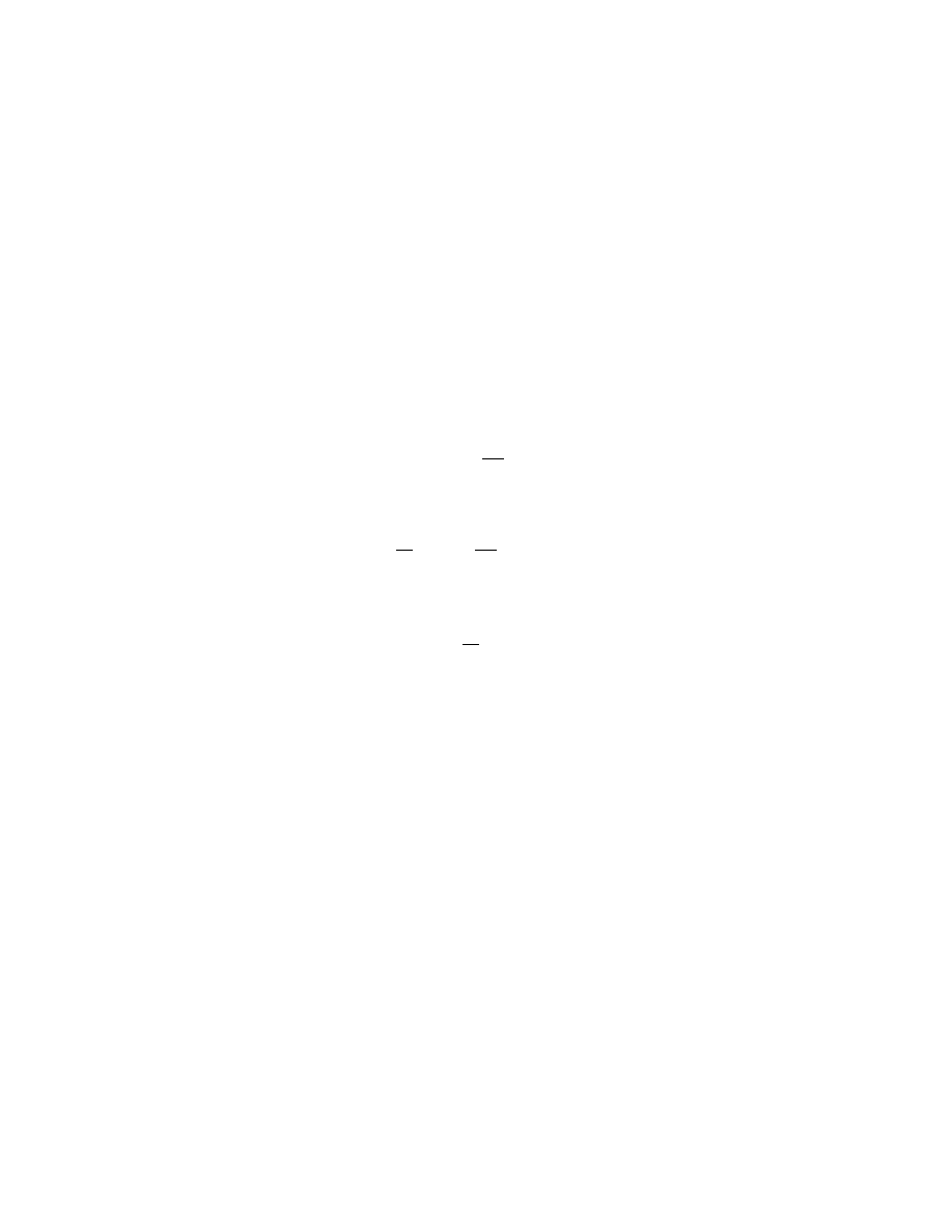
where β is a p-form on M (also depending on t) and γ is a (p−1)-form on M , depending
on t. In a coordinate system it is clear how to do this, but more invariantly, the form
β is just F
∗
t
α. To get γ in an invariant manner, we can think of
(x, s) 7→ (x, s + t)
as a local one-parameter group of diffeomorphisms of M × (a, b) which generates a
vector field X = ∂/∂t. Then
γ = i(X)F
∗
α.
Now α is closed, so from (13),
0 = d
M
β + dt ∧
∂β
∂t
− dt ∧ d
M
γ
where d
M
is the exterior derivative in the variables of M . It follows that
∂
∂t
F
∗
t
α =
∂β
∂t
= d
M
γ
so that, integrating with respect to the parameter t,
F
∗
1
α − F
∗
0
α =
Z
1
0
∂
∂t
F
∗
t
α dt = d
Z
1
0
γ dt.
So the closed forms F
∗
1
α and F
∗
0
α differ by an exact form and
F
∗
1
(a) = F
∗
0
(a).
2
Here is an immediate corollary:
Proposition 6.8 The de Rham cohomology groups of M = R
n
are zero for p > 0.
Proof: Define F : R
n
× [0, 1] → R
n
by
F (x, t) = tx.
Then F
1
(x) = x which is the identity map, and so
F
∗
1
: H
p
(R
n
) → H
p
(R
n
)
is the identity.
51

But F
0
(x) = 0 which is a constant map. In particular the derivative vanishes, so the
pull-back of any p-form of degree greater than zero is the zero map. So for p > 0
F
∗
0
: H
p
(R
n
) → H
p
(R
n
)
vanishes.
From Theorem 6.7 F
∗
0
= F
∗
1
and we deduce that H
p
(R
n
) vanishes for p > 0. Of
course R
n
is connected so H
0
(R
n
) ∼
= R.
2
Example: Show that the previous proposition holds for a star shaped region in R
n
:
an open set U with a point a ∈ U such that for each x ∈ U the straight-line segment
ax ⊂ U . This is usually called the Poincar´
e lemma.
We are in no position yet to calculate many other de Rham cohomology groups, but
here is one non-trivial example. Consider the case of R/Z, diffeomorphic to the circle.
In the atlas given earlier, we had ϕ
1
ϕ
−1
0
(x) = x or ϕ
1
ϕ
−1
0
(x) = x − 1 so the 1-form
dx = d(x − 1) is well-defined, and nowhere zero. It is not the derivative of a function,
however, since R/Z is compact and any function must have a minimum where df = 0.
We deduce that
H
1
(R/Z) 6= 0.
To get more information we need to study the other aspect of differential forms:
integration.
52
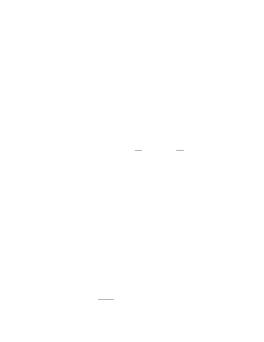
7
Integration of forms
7.1
Orientation
Recall the change of variables formula in a multiple integral:
Z
f (y
1
, . . . , y
n
)dy
1
dy
2
. . . dy
n
=
Z
f (y
1
(x), . . . , y
n
(x))| det ∂y
i
/∂x
j
|dx
1
dx
2
. . . dx
n
and compare to the change of coordinates for an n-form on an n-dimensional manifold:
θ = f (y
1
, . . . , y
n
)dy
1
∧ dy
2
∧ . . . ∧ dy
n
= f (y
1
(x), . . . , y
n
(x))
X
i
∂y
1
∂x
i
dx
i
∧ . . . ∧
X
p
∂y
n
∂x
p
dx
p
= f (y
1
(x), . . . , y
n
(x))(det ∂y
i
/∂x
j
)dx
1
∧ dx
2
. . . ∧ dx
n
The only difference is the absolute value, so that if we can sort out a consistent sign,
then we should be able to assign a coordinate-independent value to the integral of an
n-form over an n-dimensional manifold. The sign question is one of orientation.
Definition 27 An n-dimensional manifold is said to be
orientable
if it has an ev-
erywhere non-vanishing n-form ω.
Definition 28 Let M be an n-dimensional orientable manifold. An
orientation
on
M is an equivalence class of non-vanishing n-forms ω where ω ∼ ω
0
if ω
0
= f ω with
f > 0.
Clearly a connected orientable manifold has two orientations: the equivalence classes
of ±ω.
Example:
1. Let M ⊂ R
n+1
be defined by f (x) = c, with df (a) 6= 0 if f (a) = c. By Theorem
2.2, M is a manifold and moreover, if ∂f /∂x
i
6= 0, x
1
, . . . , x
i−1
, x
i+1
, x
n
are local
coordinates. Consider, on such a coordinate patch,
ω = (−1)
i
1
∂f /∂x
i
dx
1
∧ . . . ∧ dx
i−1
∧ dx
i+1
. . . ∧ dx
n
(14)
53
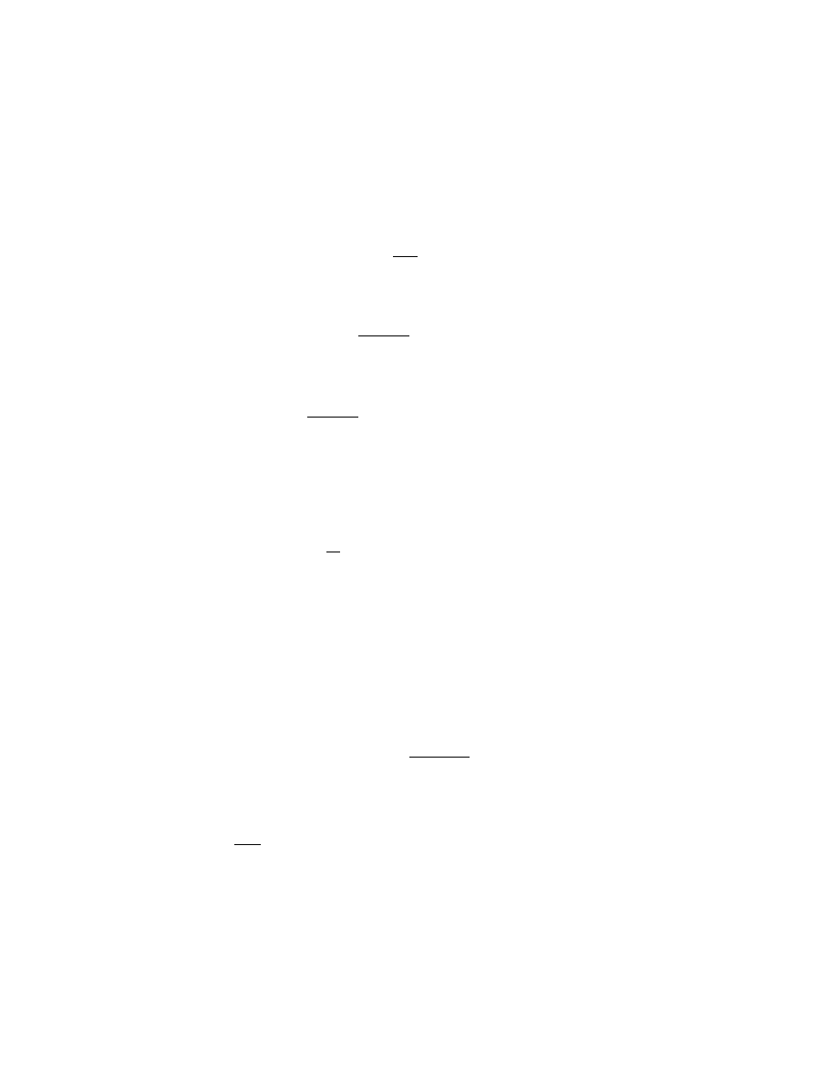
This is non-vanishing.
Now M is defined by f (x) = c so that on M
X
j
∂f
∂x
j
dx
j
= 0
and if ∂f /∂x
j
6= 0
dx
j
= −
1
∂f /∂x
j
(∂f /∂x
i
dx
i
+ . . .).
Substituting in (14) we get
ω = (−1)
j
1
∂f /∂x
j
dx
1
∧ . . . ∧ dx
j−1
∧ dx
j+1
. . . ∧ dx
n
.
The formula (14) therefore defines for all coordinate charts a non-vanishing n-form,
so M is orientable.
The obvious example is the sphere S
n
with
ω = (−1)
i
1
x
i
dx
1
∧ . . . ∧ dx
i−1
∧ dx
i+1
. . . ∧ dx
n
.
2. Consider real projective space RP
n
and the smooth map
p : S
n
→ RP
n
which maps a unit vector in R
n+1
to the one-dimensional subspace it spans. Con-
cretely, if x
1
6= 0, we use x = (x
2
, . . . , x
n+1
) as coordinates on S
n
and the usual
coordinates (x
2
/x
1
, . . . , x
n+1
/x
1
) on RP
n
, then
p(x) =
1
1 − kxk
2
x
(15)
Let σ : S
n
→ S
n
be the diffeomorphism σ(x) = −x. Then
σ
∗
ω = (−1)
i
1
−x
i
d(−x
1
) ∧ . . . ∧ d(−x
i−1
) ∧ d(−x
i+1
) . . . ∧ d(−x
n
) = (−1)
n−1
ω.
Suppose RP
n
is orientable, then it has a non-vanishing n-form θ. From (15) one finds
that the derivative of p is invertible, so that p
∗
θ is a non-vanishing n-form on S
n
and
so
p
∗
θ = f ω
54

for some non-vanishing smooth function f . But p ◦ σ = p so that
f ω = p
∗
θ = σ
∗
p
∗
θ = (f ◦ σ)(−1)
n−1
ω.
Thus, if n is even,
f ◦ σ = −f
and if f (a) > 0, f (−a) < 0. But RP
n
= p(S
n
) and S
n
is connected so RP
n
is
connected. This means that f must vanish somewhere, which is a contradiction.
Hence RP
2m
is not orientable.
Orientability helps in integration through the following:
Proposition 7.1 A manifold is orientable if and only if it has a covering by coordi-
nate charts such that
det
∂y
i
∂x
j
> 0
on the intersection.
Proof: Assume M is orientable, and let ω be a non-vanishing n-form. In a coordinate
chart
ω = f (x
1
, . . . , x
n
)dx
1
∧ . . . dx
n
.
After possibly making a coordinate change x
1
7→ c − x
1
, we have coordinates such
that f > 0.
Look at two such overlapping sets of coordinates. Then
ω = g(y
1
, . . . , y
n
)dy
1
∧ . . . ∧ dy
n
= g(y
1
(x), . . . , y
n
(x))(det ∂y
i
/∂x
j
)dx
1
∧ dx
2
. . . ∧ dx
n
= f (x
1
, . . . , x
n
)dx
1
∧ . . . dx
n
Since f > 0 and g > 0, the determinant det ∂y
i
/∂x
j
is also positive.
Conversely, suppose we have such coordinates. Take a partition of unity {ϕ
α
} subor-
dinate to the coordinate covering and put
ω =
X
ϕ
α
dy
α
1
∧ dy
α
2
∧ . . . ∧ dy
α
n
.
Then on a coordinate neighbourhood U
β
with coordinates x
1
, . . . , x
n
we have
ω|
U
β
=
X
ϕ
α
det(∂y
α
i
/∂x
j
)dx
1
∧ . . . dx
n
.
Since ϕ
α
≥ 0 and det(∂y
α
i
/∂x
j
) is positive, this is non-vanishing.
2
55

Now suppose M is orientable and we have chosen an orientation. We shall define the
integral
Z
M
θ
of any n-form θ of compact support on M .
We first choose a coordinate covering as in Proposition 7.1. On each coordinate
neighbourhood U
α
we have
θ|
U
α
= f
α
(x
1
, . . . , x
n
)dx
1
∧ . . . ∧ dx
n
.
Take a partition of unity ϕ
i
subordinate to this covering. Then
ϕ
i
θ|
U
α
= g
i
(x
1
, . . . , x
n
)dx
1
∧ . . . ∧ dx
n
where g
i
is a smooth function of compact support on the whole of R
n
. We then define
Z
M
θ =
X
i
Z
M
ϕ
i
θ =
X
i
Z
R
n
g
i
(x
1
, . . . , x
n
)dx
1
dx
2
. . . dx
n
.
Note that since θ has compact support, its support is covered by finitely many open
sets on which ϕ
i
6= 0, so the above is a finite sum.
The integral is well-defined precisely because of the change of variables formula in
integration, and the consistent choice of sign from the orientation.
7.2
Stokes’ theorem
The theorems of Stokes and Green in vector calculus are special cases of a single result
in the theory of differential forms, which by convention is called Stokes’ theorem. We
begin with a simple version of it:
Theorem 7.2 Let M be a compact, oriented n-dimensional manifold and ω ∈ Ω
n−1
(M )
be of compact support. Then
Z
M
dω = 0.
Proof: Use a partition of unity subordinate to a coordinate covering to write
ω =
X
ϕ
i
ω.
56
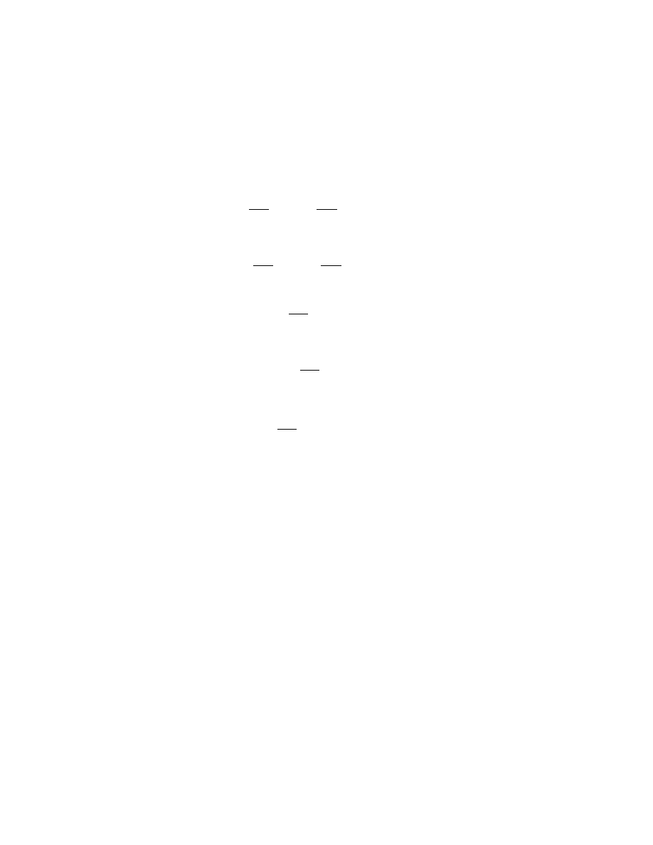
Then on a coordinate neighbourhood
ϕ
i
ω = a
1
dx
2
∧ . . . ∧ dx
n
− a
2
dx
1
∧ dx
3
∧ . . . ∧ dx
n
+ . . .
and
d(ϕ
i
ω) =
∂a
1
∂x
1
+ . . . +
∂a
n
∂x
n
dx
1
∧ dx
2
∧ . . . ∧ dx
n
.
From the definition of the integral, we need to sum each
Z
R
n
∂a
1
∂x
1
+ . . . +
∂a
n
∂x
n
dx
1
dx
2
. . . dx
n
.
Consider
Z
R
n
∂a
1
∂x
1
dx
1
dx
2
. . . dx
n
.
By Fubini’s theorem we evaluate this as a repeated integral
Z
R
Z
R
. . .
Z
∂a
1
∂x
1
dx
1
dx
2
dx
3
. . . dx
n
.
But a
1
has compact support, so vanishes if |x
1
| ≥ N and thus
Z
R
∂a
1
∂x
1
dx
1
= [a
1
]
N
−N
= 0.
The other terms vanish in a similar way.
2
Theorem 7.2 has an immediate payoff for de Rham cohomology:
Proposition 7.3 Let M be a compact orientable n-dimensional manifold. Then the
de Rham cohomology group H
n
(M ) is non-zero.
Proof:
Since M is orientable, it has a non-vanishing n-form θ. Because there are
no n + 1-forms, it is closed, and defines a cohomology class [θ] ∈ H
n
(M ).
Choose the orientation defined by θ and integrate: we get
Z
M
θ =
X
Z
f
i
dx
1
dx
2
. . . dx
n
which is positive since each f
i
≥ 0 and is positive somewhere.
Now if the cohomology class [θ] = 0, θ = dω, but then Theorem 7.2 gives
Z
M
θ =
Z
M
dω = 0
a contradiction.
2
57

Here is a topological result which follows directly from the proof of the above fact:
Theorem 7.4 Every vector field on an even-dimensional sphere S
2m
vanishes some-
where.
Proof:
Suppose for a contradiction that there is a non-vanishing vector field. For
the sphere, sitting inside R
2m+1
, we can think of a vector field as a smooth map
v : S
2m
→ R
2m+1
such that (x, v(x)) = 0 and if v is non-vanishing we can normalize it to be a unit
vector. So assume (v(x), v(x)) = 1.
Now define F
t
: S
2m
→ R
2m+1
by
F
t
(x) = cos t x + sin t v(x).
Since (x, v(x)) = 0, we have
(cos t x + sin t v(x), cos t x + sin t v(x)) = 1
so that F
t
maps the unit sphere to itself. Moreover,
F
0
(x) = x,
F
π
(x) = −x.
Now let ω be the standard orientation form on S
2m
:
ω = dx
1
∧ dx
2
∧ . . . ∧ dx
2m
/x
2m+1
.
We see that
F
∗
0
ω = ω,
F
∗
π
ω = −ω.
But by Theorem 6.7, the maps F
∗
0
, F
∗
π
on H
2m
(S
2m
) are equal. We deduce that the
de Rham cohomology class of ω is equal to its negative and so must be zero, but this
contradicts that fact that its integral is positive. Thus the vector field must have a
zero.
2
Green’s theorem relates a surface integral to a volume integral, and the full version of
Stokes’ theorem does something similar for manifolds. The manifolds we have defined
are analogues of a surface – the sphere for example. We now need to find analogues
of the solid ball that the sphere bounds. These are still called manifolds, but with a
boundary.
58
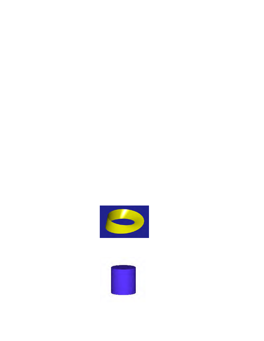
Definition 29 An n-dimensional
manifold with boundary
is a set M with a collec-
tion of subsets U
α
and maps
ϕ
α
: U
α
→ (R
n
)
+
= {(x
1
, . . . , x
n
) ∈ R
n
: x
n
≥ 0}
such that
• M = ∪
α
U
α
• ϕ
α
: U
α
→ ϕ
α
(U
α
) is a bijection onto an open set of (R
n
)
+
and ϕ
α
(U
α
∩ U
β
) is
open for all α, β,
• ϕ
β
ϕ
−1
α
: ϕ
α
(U
α
∩ U
β
) → ϕ
β
(U
α
∩ U
β
) is the restriction of a C
∞
map from a
neighbourhood of ϕ
α
(U
α
∩ U
β
) ⊆ (R
n
)
+
⊂ R
n
to R
n
.
The
boundary
∂M of M is defined as
∂M = {x ∈ M : ϕ
α
(x) ∈ {(x
1
, . . . , x
n−1
, 0) ∈ R
n
}
and these charts define the structure of an (n − 1)-manifold on ∂M .
Example:
1. The model space (R
n
)
+
is a manifold with boundary x
n
= 0.
2. The unit ball {x ∈ R
n
: kxk ≤ 1} is a manifold with boundary S
n−1
.
3. The M¨
obius band is a 2-dimensional manifold with boundary the circle:
4. The cylinder I × S
1
is a 2-dimensional manifold with boundary the union of two
circles – a manifold with two components.
59

We can define differential forms etc. on manifolds with boundary in a straightforward
way. Locally, they are just the restrictions of smooth forms on some open set in R
n
to (R
n
)
+
. A form on M restricts to a form on its boundary.
Proposition 7.5 If a manifold M with boundary is oriented, there is an induced
orientation on its boundary.
Proof: We choose local coordinate systems such that ∂M is defined by x
n
= 0 and
det(∂y
i
/∂x
j
) > 0. So, on overlapping neighbourhoods,
y
i
= y
i
(x
1
, . . . , x
n
),
y
n
(x
1
, . . . , x
n−1
, 0) = 0.
Then the Jacobian matrix has the form
∂y
1
/∂x
1
∂y
1
/∂x
2
∂y
1
/∂x
n
. . .
. . .
. . .
. . .
. . .
. . .
. . .
. . .
. . .
. . .
. . .
. . .
0
0
0
∂y
n
/∂x
n
(16)
From the definition of manifold with boundary, ϕ
β
ϕ
−1
α
maps x
n
> 0 to y
n
> 0, so y
n
has the property that if x
n
= 0, y
n
= 0 and if x
n
> 0, y
n
> 0. It follows that
∂y
n
∂x
n
x
n
=0
> 0.
From (16) the determinant of the Jacobian for ∂M is given by
det(J
∂M
)
∂y
n
∂x
n
x
n
=0
= det(J
M
)
so if det(J
M
) > 0 so is det(J
∂M
).
2
Remark:
The boundary of an oriented manifold has an induced orientation, but
there is a convention about which one to choose: for a surface in R
3
this is the choice
of an “inward” or “outward” normal. Our choice will be that if dx
1
∧ . . . ∧ dx
n
defines
the orientation on M with x
n
≥ 0 defining M locally, then −dx
1
∧ . . . ∧ dx
n−1
(the
“outward” normal) is the induced orientation on ∂M . The boundary of the cylinder
gives opposite orientations on the two circles. The M¨
obius band is not orientable,
though its boundary the circle of course is.
60

We can now state the full version of Stokes’theorem:
Theorem 7.6 (Stokes’ theorem) Let M be an n-dimensional oriented manifold with
boundary ∂M and let ω ∈ Ω
n−1
(M ) be a form of compact support. Then, using the
induced orientation
Z
M
dω =
Z
∂M
ω.
Proof: We write again
ω =
X
ϕ
i
ω
and then
Z
M
dω =
X
Z
M
d(ϕ
i
ω).
We work as in the previous version of the theorem (7.2), but now there are two types
of open sets. For those which do not intersect ∂M the integral is zero by Theorem
7.2. For those which do, we have
Z
M
d(ϕ
i
ω) = −
Z
x
n
≥0
∂a
1
∂x
1
+ . . . +
∂a
n
∂x
n
dx
1
dx
2
. . . dx
n
= −
Z
[a
n
]
∞
0
dx
1
. . . dx
n−1
=
Z
∂M
ϕ
i
ω
2
An immediate corollary is the following classical result, called the Brouwer fixed point
theorem.
Theorem 7.7 Let B be the unit ball {x ∈ R
n
: kxk ≤ 1} and let F : B → B be a
smooth map from B to itself. Then F has a fixed point.
Proof:
Suppose there is no fixed point, so that F (x) 6= x for all x ∈ B. For each
x ∈ B, extend the straight line segment F (x)x until it meets the boundary sphere of
B in the point f (x). Then we have a smooth function
f : B → ∂B
such that if x ∈ ∂B, f (x) = x.
61

Let ω be the standard non-vanishing (n − 1)-form on S
n−1
= ∂B, with
Z
∂B
ω = 1.
Then
1 =
Z
∂B
ω =
Z
∂B
f
∗
ω
since f is the identity on S
n−1
. But by Stokes’ theorem,
Z
∂B
f
∗
ω =
Z
B
d(f
∗
ω) =
Z
B
f
∗
(dω) = 0
since dω = 0 as ω is in the top dimension on S
n−1
.
The contradiction 1 = 0 means that there must be a fixed point.
2
8
The degree of a smooth map
By using integration of forms we have seen that for a compact orientable manifold of
dimension n the de Rham cohomology group H
n
(M ) is non-zero, and that this fact
enabled us to prove some global topological results about such manifolds. We shall
now refine this result, and show that the group is (for a compact, connected, orientable
manifold) just one-dimensional. This gives us a concrete method of determining the
cohomology class of an n-form: it is exact if and only if its integral is zero.
8.1
de Rham cohomology in the top dimension
First a lemma:
Lemma 8.1 Let U
n
= {x ∈ R
n
: |x
i
| < 1} and let ω ∈ Ω
n
(R
n
) be a form with
support in U
n
such that
Z
U
n
ω = 0.
Then there exists β ∈ Ω
n−1
(R
n
) with support in U
n
such that ω = dβ.
Proof:
We prove the result by induction on the dimension n, but we make the
inductive assumption that ω and β depend smoothly on a parameter λ ∈ R
m
, and
also that if ω vanishes identically for some λ, so does β.
62

Consider the case n = 1, so ω = f (x, λ)dx. Clearly taking
β(x, λ) =
Z
x
−1
f (u, λ)du
(17)
gives us a function with dβ = ω. But also, since f has support in U ,
Z
1−δ
−1+δ
f (u, λ)du = 0
so we have β(x, λ) = 0 if |x| > 1 − δ and β itself has support in U . If f (x, λ) = 0 for
all x, then from the integration (17) so does β(x, λ).
Now assume the result for dimensions less than n and let
ω = f (x
1
, . . . , x
n
, λ)dx
1
∧ . . . ∧ dx
n
be the given form. Fix x
n
= t and consider
f (x
1
, . . . , x
n−1
, t, λ)dx
1
∧ . . . ∧ dx
n−1
as a form on R
n−1
, depending smoothly on t and λ. Its integral is no longer zero, but
if σ is a bump function on U
n−1
with integral 1, then putting
g(t, λ) =
Z
f (x
1
, . . . , x
n−1
, t, λ)dx
1
∧ . . . ∧ dx
n−1
we have a form
f (x
1
, . . . , x
n−1
, t, λ)dx
1
∧ . . . ∧ dx
n−1
− g(t, λ)σ
with support in U
n−1
and zero integral. Apply induction to this and we can write it
as dγ where γ has support in U
n−1
.
Now put t = x
n
, and consider d(γ ∧ dx
n
). The x
n
-derivative of γ doesn’t contribute
because of the dx
n
factor, so we get
d(γ ∧ dx
n
) = f (x
1
, . . . , x
n−1
, x
n
, λ)dx
1
∧ . . . ∧ dx
n
− g(x
n
, λ)σ ∧ dx
n
.
Putting
ξ(x
1
, . . . , x
n
, λ) = (−1)
n−1
(
Z
x
n
0
g(t, λ)dt)σ
also gives
dξ = g(x
n
, λ)σ ∧ dx
n
.
63

We can therefore write
f (x
1
, . . . , x
n−1
, x
n
, λ)dx
1
∧ . . . ∧ dx
n
= d(γ ∧ dx
n
+ ξ) = dβ.
Now by construction β has support in |x
i
| < 1 for 1 ≤ i ≤ n − 1, but what about
the x
n
direction? Since f (x
1
, . . . , x
n−1
, t, λ) vanishes for t > 1 − δ or t < −1 + δ, the
inductive assumption tells us that γ does also for x
n
> 1 − δ. As for ξ, if t > 1 − δ,
Z
t
0
g(s, λ)ds =
Z
t
0
Z
U
n−1
f (x
1
, . . . , x
n−1
, t, λ)dx
1
∧ . . . ∧ dx
n−1
dt
=
Z
1
0
Z
U
n−1
f (x
1
, . . . , x
n−1
, t, λ)dx
1
∧ . . . ∧ dx
n−1
dt
=
Z
U
n
f (x
1
, . . . , x
n
, λ) dx
1
∧ . . . ∧ dx
n
= 0
by assumption. Thus the support of ξ is in U
n
. Again, examining the integrals, if
f (x, λ) is identically zero for some λ, so is β.
2
Using the lemma, we prove:
Theorem 8.2 If M is a compact, connected orientable n-dimensional manifold, then
H
n
(M ) ∼
= R.
Proof:
Take a covering by coordinate neighbourhoods which map to U
n
= {x ∈
R
n
: |x
i
| < 1} and a corresponding partition of unity {ϕ
i
}. By compactness, we can
assume we have a finite number U
1
, . . . , U
N
of open sets. Using a bump function, fix
an n-form α
0
with support in U
1
and
Z
M
α
0
= 1.
Thus, by Theorem 7.3 the cohomology class [α
0
] is non-zero. To prove the theorem
we want to show that for any n-form α,
[α] = c[α
0
]
i.e. that α = cα
0
+ dγ.
64

Given α use the partition of unity to write
α =
X
ϕ
i
α
then by linearity it is sufficient to prove the result for each ϕ
i
α, so we may assume
that the support of α lies in a coordinate neighbourhood U
m
. Because M is connected
we can connect p ∈ U
1
and q ∈ U
m
by a path and by the connectedeness of open
intervals we can assume that the path is covered by a sequence of U
i
’s, each of which
intersects the next: i.e. renumbering, we have
p ∈ U
1
,
U
i
∩ U
i+1
6= ∅,
q ∈ U
m
.
Now for 1 ≤ i ≤ m − 1 choose an n-form α
i
with support in U
i
∩ U
i+1
and integral 1.
On U
1
we have
Z
(α
0
− α
1
) = 0
and so applying Lemma 8.1, there is a form β
0
with support in U
1
such that
α
0
− α
1
= dβ
1
.
Continuing, we get
α
0
− α
1
= dβ
1
α
1
− α
2
= dβ
2
. . . = . . .
α
m−2
− α
m−1
= dβ
m−1
and adding, we get
α
0
− α
m−1
= d(
X
i
β
i
)
(18)
On U
m
, we have
Z
α = c =
Z
cα
m−1
and applying the Lemma again, we get α − cα
m−1
= dβ and so from (18)
α = cα
m−1
+ dβ = cα
0
+ d(β − c
X
i
β
i
)
as required.
2
65

Theorem 8.2 tells us that for a compact connected oriented n-dimensional manifold,
H
n
(M ) is one-dimensional. Take a form ω
M
whose integral over M is 1, then [ω
M
] is
a natural basis element for H
n
(M ). Suppose
F : M → N
is a smooth map of compact connected oriented manifolds of the same dimension n.
Then we have the induced map
F
∗
: H
n
(N ) → H
n
(M )
and relative to our bases
F
∗
[ω
N
] = d[ω
M
]
(19)
for some real number d. We now show that d is an integer.
Theorem 8.3 Let M , N be oriented, compact, connected manifolds of the same di-
mension n, and F : M → N a smooth map. There exists an integer, called the
degree
of F such that
• if ω ∈ Ω
n
(N ) then
Z
M
F
∗
ω = deg F
Z
N
ω
• if a is a regular value of F then
deg F =
X
x∈F
−1
(a)
sgn(det DF
x
)
Remark:
1. A regular value for a smooth map F : M → N is a point a ∈ N such that for each
x ∈ F
−1
(a), the derivative DF
x
is surjective. When dim M = dim N this means that
DF
x
is invertible. Sard’s theorem (a proof of which is in the Appendix) shows that
for any smooth map most points in N are regular values.
2. The expression sgn(det DF
x
) in the theorem can be interpreted in two ways, but
depends crucially on the notion of orientation – consistently associating the right
sign for all the points x ∈ F
−1
(a). The straightforward approach uses Proposition
7.1 to associate to an orientation a class of coordinates whose Jacobians have positive
determinant. If det DF
x
is written as a Jacobian matrix in such a set of coordinates
66

for M and N , then sgn(det DF
x
) is just the sign of the determinant. More invariantly,
DF
x
: T
x
M 7→ T
a
N defines a linear map
Λ
n
(DF
0
x
) : ΛT
∗
N
a
→ ΛT
∗
x
M.
Orientations on M and N are defined by non-vanishing forms ω
M
, ω
N
and
Λ
n
(DF
0
x
)(ω
N
) = λω
M
.
Then sgn(det DF
x
) is the sign of λ.
3. Note the immediate corollary of the theorem: if F is not surjective, then deg F = 0.
Proof:
For the first part of the theorem, the cohomology class of ω is [ω] = c[ω
N
]
and so integrating (and using Proposition 7.2,
Z
N
ω = c
Z
N
ω
N
= c.
Using the number d in (19),
F
∗
[ω] = cF
∗
[ω
N
] = cd[ω
M
]
and integrating,
Z
M
F
∗
ω = cd
Z
M
ω
M
= cd = d
Z
N
ω.
For the second part, since DF
x
is an isomorphism at all points in F
−1
(a), from
Theorem 3.3, F
−1
(a) is a zero-dimensional manifold. Since it is compact (closed
inside a compact space M ) it is a finite set of points. The inverse function theorem
applied to these m points shows that there is a coordinate neighbourhood U of a ∈ N
such that F
−1
(U ) is a disjoint union of m open sets U
i
such that
F : U
i
→ U
is a diffeomorphism.
Let σ be an n-form supported in U with
R
N
σ = 1 and consider the diffeomorphism
F : U
i
→ U . Then by the coordinate invariance of integration of forms, and using
the orientations on M and N ,
Z
U
i
F
∗
σ = sgn DF
x
i
Z
U
σ = sgn DF
x
i
.
67

Hence, summing
Z
M
F
∗
σ =
X
i
sgn DF
x
i
and this is from the first part
d = d
Z
N
σ =
Z
M
F
∗
σ
which gives
d =
X
i
sgn DF
x
i
.
2
Example:
Let M be the extended complex plane: M = C ∪ {∞}. This is a
compact, connected, orientable 2-manifold. In fact it is the 2-sphere. Consider the
map F : M → M defined by
F (z) = z
k
+ a
1
z
k−1
+ . . . + a
k
,
z 6= ∞
F (∞) = ∞
This is smooth because in coordinates near z = ∞, F is defined (for w = 1/z by
w 7→
w
k
1 + a
1
w + . . . a
k
w
k
.
To find the degree of F , consider
F
t
(z) = z
k
+ t(a
1
z
k−1
+ . . . + a
k
).
This is a smooth map for all t and by Theorem 6.7 the action on cohomology is
independent of t, so
deg F = deg F
0
where F
0
(z) = z
k
.
We can calculate this degree by taking a 2-form, with |z| = r and z = x + iy
f (r)dx ∧ dy = f (r)rdr ∧ dθ
with f (r) of compact support. Then the degree is given by
deg F
0
Z
R
2
f (r)rdr ∧ dθ =
Z
R
2
f (r
k
)r
k
d(r
k
)kdθ = k
Z
R
2
f (r)rdr ∧ dθ.
68

Thus deg F = k. If k > 0 this means in particular that F is surjective and in
particular takes the value 0 somewhere, so that
z
k
+ a
1
z
k−1
+ . . . + a
k
= 0
has a solution. This is the fundamental theorem of algebra.
Example:
Take two smooth maps f
1
, f
2
: S
1
→ R
3
. These give two circles in R
3
.
Define
F : S
1
× S
1
→ S
2
by
F (s, t) =
f
1
(s) − f
2
(t)
kf
1
(s) − f
2
(t)k
.
The degree of this map is called the linking number.
Example:
Let M ⊂ R
3
be a compact surface and n its unit normal. The Gauss
map is the map
F : M → S
2
defined by F (x) = n(x). If we work out the degree by integration, we take the
standard 2-form ω on S
2
. Then one finds that
Z
M
F
∗
ω =
Z
M
K
√
EG − F
2
dudv
where K is the Gaussian curvature. The degree tells us this integral is 2π times an
integer, which by the Gauss-Bonnet theorem is the Euler characteristic of M .
69

9
Riemannian metrics
Differential forms and the exterior derivative provide one piece of analysis on mani-
folds which, as we have seen, links in with global topological questions. There is much
more one can do when one introduces a Riemannian metric. Since the whole subject
of Riemannian geometry is a huge one, we shall here look at only two aspects which
relate to the use of differential forms: the study of harmonic forms and of geodesics.
In particular, we ignore completely here questions related to curvature.
9.1
The metric tensor
In informal terms, a Riemannian metric on a manifold M is a smoothly varying
positive definite inner product on the tangent spaces T
x
. To make global sense of
this, note that an inner product is a bilinear form, so at each point x we want a
vector in the tensor product
T
∗
x
⊗ T
∗
x
.
We can put, just as we did for the exterior forms, a vector bundle structure on
T
∗
M ⊗ T
∗
M =
[
x∈M
T
∗
x
⊗ T
∗
x
.
The conditions we need to satisfy for a vector bundle are provided by two facts we
used for the bundle of p-forms:
• each coordinate system x
1
, . . . , x
n
defines a basis dx
1
, . . . , dx
n
for each T
∗
x
in the
coordinate neighbourhood and the n
2
elements
dx
i
⊗ dx
j
,
1 ≤ i, j ≤ n
give a corresponding basis for T
∗
x
⊗ T
∗
x
• the Jacobian of a change of coordinates defines an invertible linear map J : T
∗
x
→
T
∗
x
and we have a corresponding invertible map J ⊗ J : T
∗
x
⊗ T
∗
x
→ T
∗
x
⊗ T
∗
x
.
Given this, we define:
Definition 30 A
Riemannian metric
on a manifold M is a section g of T
∗
⊗ T
∗
which at each point is symmetric and positive definite.
70

In a local coordinate system we can write
g =
X
i,j
g
ij
(x)dx
i
⊗ dx
j
where g
ij
(x) = g
ji
(x) and is a smooth function, with g
ij
(x) positive definite. Often
the tensor product symbol is omitted and one simply writes
g =
X
i,j
g
ij
(x)dx
i
dx
j
.
Example:
1. The Euclidean metric on R
n
is defined by
g =
X
dx
i
⊗ dx
i
.
So
g(
∂
∂x
i
,
∂
∂x
j
) = δ
ij
.
2. A submanifold of R
n
has an induced Riemannian metric: the tangent space at x
can be thought of as a subspace of R
n
and we take the Euclidean inner product on
R
n
.
Given a smooth map F : M → N and a metric g on N , we can pull back g to a
section F
∗
g of T
∗
M ⊗ T
∗
M :
(F
∗
g)
x
(X, Y ) = g
F
(x)(DF
x
(X), DF
x
(Y )).
If DF
x
is invertible, this will again be positive definite, so in particular if F is a
diffeomorphism.
Definition 31 A diffeomorphism F : M → N between two Riemannian manifolds is
an
isometry
if F
∗
g
N
= g
M
.
Example: Let M = {(x, y) ∈ R
2
: y > 0} and
g =
dx
2
+ dy
2
y
2
.
If z = x + iy and
F (z) =
az + b
cz + d
71

with a, b, c, d real and ad − bc > 0, then
F
∗
dz = (ad − bc)
dz
(cz + d)
2
and
F
∗
y = y ◦ F =
1
i
az + b
cz + d
−
a¯
z + b
c¯
z + d
=
ad − bc
|cz + d|
2
y.
Then
F
∗
g = (ad − bc)
2
dx
2
+ dy
2
|(cz + d)
2
|
2
|cz + d|
4
(ad − bc)
2
y
2
=
dx
2
+ dy
2
y
2
= g.
So these M¨
obius transformations are isometries of a Riemannian metric on the upper
half-plane.
This is the non-Euclidean geometry dealt with in the Projective Geometry Notes.
With a Riemannian metric one can define the length of a curve:
Definition 32 Let M be a Riemannian manifold and γ : [0, 1] → M a smooth map
(i.e. a smooth curve in M ). The
length
of the curve is
`(γ) =
Z
1
0
p
g(γ
0
, γ
0
)dt
where γ
0
(t) = Dγ
t
(d/dt).
With this definition, any Riemannian manifold is a metric space: define
d(x, y) = inf{`(γ) ∈ R : γ(0) = x, γ(1) = y}.
Are Riemannian manifolds special? No, because:
Proposition 9.1 Any manifold admits a Riemannian metric.
Proof:
Take a covering by coordinate neighbourhoods and a partition of unity
subordinate to the covering. On each open set U
α
we have a metric
g
α
=
X
i
dx
2
i
in the local coordinates. Define
g =
X
ϕ
i
g
α(i)
.
This sum is well-defined because the supports of ϕ
i
are locally finite. Since ϕ
i
≥ 0
at each point every term in the sum is positive definite or zero, but at least one is
positive definite so the sum is positive definite.
2
72

9.2
The geodesic flow
Consider any manifold M and its cotangent bundle T
∗
M , with projection p : T
∗
M →
M . Let X be tangent vector to T
∗
M at the point ξ
a
∈ T
∗
a
. Then
Dp
ξ
a
(X) ∈ T
a
M
so
θ(X) = ξ
a
(Dp
ξ
a
(X))
defines a canonical 1-form θ on T
∗
M . In coordinates (x, y) 7→
P
i
y
i
dx
i
, the projection
p is
p(x, y) = x
so if
X =
X
a
i
∂
∂x
i
+
X
b
i
∂
∂y
i
then
θ(X) =
X
i
y
i
dx
i
(Dp
ξ
a
X) =
X
i
y
i
a
i
which gives
θ =
X
i
y
i
dx
i
.
We now take the exterior derivative
ω = −dθ =
X
dx
i
∧ dy
i
which is the canonical 2-form on the cotangent bundle. It is non-degenerate, so that
the map
X 7→ i(X)ω
from the tangent bundle of T
∗
M to its cotangent bundle is an isomorphism.
Now suppose f is a smooth function on T
∗
M . Its derivative is a 1-form df . Because
of the isomorphism above, there is a unique vector field X on T
∗
M such that
i(X)ω = df.
If g is another function with vector field Y , then
Y (f ) = df (Y ) = i(Y )i(X)ω = −i(X)i(Y )ω = −X(g)
(20)
73

On a Riemannian manifold we shall see next that there is a natural function on T
∗
M .
In fact a metric defines an inner product on T
∗
as well as on T , for the map
X 7→ g(X, −)
defines an isomorphism from T to T
∗
. In concrete terms, if g
∗
is the inner product
on T
∗
, then
g
∗
(
X
j
g
ij
dx
j
,
X
k
g
kl
dx
l
) = g
ik
which means that
g
∗
(dx
j
, dx
k
) = g
jk
where g
jk
denotes the inverse matrix to g
jk
.
We consider the function on T
∗
M defined by
H(ξ
a
) = g
∗
(ξ
a
, ξ
a
).
In local coordinates this is
H(x, y) =
X
ij
g
ij
(x)y
i
y
j
.
Definition 33 The vector field X on T
∗
M given by i(X)ω = dH is called the
geodesic
flow
of the metric g.
Definition 34 If γ : (a, b) → T
∗
M is an integral curve of the geodesic flow, then the
curve p(γ) in M is called a
geodesic
.
In local coordinates, if the geodesic flow is
X =
X
a
i
∂
∂x
i
+
X
b
i
∂
∂y
i
then
i(X)ω =
X
k
(a
k
dy
k
− b
k
dx
k
) = dH =
X
ij
∂g
ij
∂x
k
dx
k
y
i
y
j
+ 2
X
ij
g
ij
y
i
dy
j
.
Thus the integral curves are solutions of
dx
k
dt
= 2
X
j
g
kj
y
j
(21)
dy
k
dt
= −
X
ij
∂g
ij
∂x
k
y
i
y
j
(22)
74
Before we explain why this is a geodesic, just note the qualitative behaviour of these
curves. For each point a ∈ M , choose a point ξ
a
∈ T
∗
a
and consider the unique
integral curve starting at ξ
a
. Equation (21) tells us that the projection of the integral
curve is parallel at a to the tangent vector X
a
such that g(X
a
, −) = ξ
a
. Thus these
curves have the property that through each point and in each direction there passes
one geodesic.
Geodesics are normally thought of as curves of shortest length, so next we shall link
up this idea with the definition above. Consider the variational problem of looking
for critical points of the length functional
`(γ) =
Z
1
0
p
g(γ
0
, γ
0
)dt
for curves with fixed end-points γ(0) = a, γ(1) = b. For simplicity assume a, b are in
the same coordinate neighbourhood. If
F (x, z) =
X
ij
g
ij
(x)z
i
z
j
then the first variation of the length is
δ` =
Z
1
0
1
2
F
−1/2
∂F
∂x
i
˙x
i
+
∂F
∂z
i
d ˙x
i
dt
dt
=
Z
1
0
1
2
F
−1/2
∂F
∂x
i
˙x
i
−
d
dt
1
2
F
−1/2
∂F
∂z
i
˙x
i
dt.
on integrating by parts with ˙x
i
(0) = ˙x
i
(1) = 0. Thus a critical point of the functional
is given by
1
2
F
−1/2
∂F
∂x
i
−
d
dt
1
2
F
−1/2
∂F
∂z
i
= 0
If we parametrize this critical curve by arc length:
s =
Z
t
0
p
g(γ
0
, γ
0
)dt
then F = 1, and the equation simplifies to
∂F
∂x
i
−
d
dt
∂F
∂z
i
= 0.
But this is
X
∂g
jk
∂x
i
dx
j
dt
dx
k
dt
−
d
dt
2g
ik
dx
k
dt
= 0
(23)
75
But now define y
i
by
dx
k
dt
= 2
X
j
g
kj
y
j
as in the first equation for the geodesic flow (21) and substitute in (23) and we get
4
X
∂g
jk
∂x
i
g
ja
y
a
g
kb
y
b
−
d
dt
4g
ik
g
ka
y
a
= 0
and using
X
j
g
ij
g
jk
= δ
i
k
this yields
−
∂g
jk
∂x
i
y
j
y
k
=
dy
i
dt
which is the second equation for the geodesic flow. (Here we have used the formula
for the derivative of the inverse of a matrix G: D(G
−1
) = −G
−1
DGG
−1
).
The formalism above helps to solve the geodesic equations when there are isometries
of the metric. If F : M → M is a diffeomorphism of M then its natural action on
1-forms induces a diffeomorphism of T
∗
M . Similarly with a one-parameter group ϕ
t
.
Differentiating at t = 0 this means that a vector field X on M induces a vector field ˜
X
on T
∗
M . Moreover, the 1-form θ on T
∗
M is canonically defined and hence invariant
under the induced action of any diffeomorphism. This means that
L
˜
X
θ = 0
and therefore, using (6.5) that
i( ˜
X)dθ + d(i( ˜
X)θ) = 0
so since ω = −dθ
i( ˜
X)ω = df
where f = i( ˜
X)θ.
Proposition 9.2 Any vector field Y on T
∗
M for which L
Y
θ = 0 is the vector field
˜
X induced from a vector field X on M . The function f = i( ˜
X)θ is f (ξ
x
) = ξ
x
(X
x
).
Proof: Write in coordinates
Y =
X
a
i
∂
∂x
i
+
X
b
i
∂
∂y
i
76
where θ =
P
i
y
i
dx
i
then L
Y
θ = 0 gives
0 =
X
i
b
i
dx
i
+
X
i,j
y
i
(
∂a
i
∂x
j
dx
j
+
∂a
i
∂y
j
dy
j
).
This implies that a
i
is independent of y
i
and so
X =
X
i
a
i
∂
∂x
i
is the required vector field X on M . We have
i( ˜
X)θ =
X
i
a
i
(x)y
i
= ξ
x
(X
x
)
by the definition of θ.
2
Now let M be a Riemannian manifold and H the function on T
∗
M defined by the
metric as above. If ϕ
t
is a one-parameter group of isometries, then the induced
diffeomorphisms of T
∗
M will preserve the function H and so the vector field ˜
Y will
satisfy
˜
Y (H) = 0.
But from (20) this means that X(f ) = 0 where X is the geodesic flow and f the
function i( ˜
Y )θ. This function is constant along the geodesic flow, and is therefore a
constant of integration of the geodesic equations.
Example: Consider the metric
g =
dx
2
1
+ dx
2
2
x
2
2
on the upper half plane and its geodesic flow X.
The map (x
1
, x
2
) 7→ (x
1
+ t, x
2
) is clearly a one-parameter group of isometries (the
M¨
obius transformations z 7→ z + t) and defines the vector field
Y =
∂
∂x
1
.
On the cotangent bundle this gives the function
f (x, y) = y
1
77

which is constant on the integral curve.
The map z 7→ e
t
z is also an isometry with vector field
Z = x
1
∂
∂x
1
+ x
2
∂
∂x
2
so that
g(x, y) = x
1
y
1
+ x
2
y
2
is constant.
We also have automatically that H = x
2
2
(y
2
1
+ y
2
2
) is constant since
X(H) = i(X)i(X)ω = 0.
We therefore have three equations for the integral curves of the geodesic flow:
y
1
= c
1
x
1
y
1
+ x
2
y
2
= c
2
x
2
2
(y
2
1
+ y
2
2
) = c
3
Eliminating y
1
, y
2
gives the geodesics:
(c
1
x
1
− c
2
)
2
+ c
2
1
x
2
2
= c
3
.
If c
1
= 0 this is a half-line x
2
= const.. Otherwise it is a semicircle with centre on
the x
1
axis. These are the straight lines of non-Euclidean geometry as described in
the Projective Geometry notes.
9.3
Harmonic forms
We mentioned above that a metric g defines an inner product not just on T
a
but also
an inner product g
∗
on T
∗
a
. With this we can define an inner product on the pth
exterior power Λ
p
T
∗
a
:
(α
1
∧ α
2
∧ . . . ∧ α
p
, β
1
∧ β
2
∧ . . . ∧ β
p
) = det g
∗
(α
i
, β
j
)
(24)
In particular, on an n-manifold there is an inner product on each fibre of the bundle
Λ
n
T
∗
. Since each fibre is one-dimensional there are only two unit vectors ±u.
Definition 35 Let M be an oriented Riemannian manifold, then the
volume form
is
the unique n-form ω of unit length in the equivalence class defined by the orientation.
78

In local coordinates,the definition of the inner product (24) gives
(dx
1
∧ . . . ∧ dx
n
, dx
1
∧ . . . ∧ dx
n
) = det g
∗
ij
= (det g
ij
)
−1
Thus if dx
1
∧ . . . ∧ dx
n
defines the orientation,
ω =
pdet g
ij
dx
1
∧ . . . ∧ dx
n
.
On a compact manifold we can integrate this to obtain the total volume – so a metric
defines not only lengths but also volumes.
Now take α ∈ Λ
p
T
∗
a
, β ∈ Λ
n−p
T
∗
a
and define f
β
: Λ
p
T
∗
a
→ R by
f
β
(α)ω = β ∧ α.
But we have an inner product, so any linear map on Λ
p
T
∗
a
is of the form
α 7→ (α, γ)
for some γ ∈ Λ
p
T
∗
a
, so we have a well-defined linear map β 7→ γ
β
from Λ
n−p
T
∗
to
Λ
p
T
∗
, satisfying
(γ
β
, α)ω = β ∧ α.
We use a different symbol for this:
Definition 36 The
Hodge star operator
is the linear map ∗ : Ω
p
(M ) → Ω
n−p
(M )
with the property that at each point
(α, β)ω = α ∧ ∗β.
Example: If e
1
, . . . , e
n
is an orthonormal basis of the space of one-forms at a point,
then
∗(e
1
∧ . . . ∧ e
p
) = e
p+1
∧ . . . ∧ e
n
.
Exercise 9.3 Show that on p-forms, ∗
2
= (−1)
p(n−p)
.
On a Riemannian manifold we can use the star operator to define new differential
operators on forms. In particular, consider the operator
d
∗
: Ω
p
(M ) → Ω
p−1
(M )
defined by
d
∗
= (−1)
np+n+1
∗ d ∗ .
The notation is suggestive, in fact:
79

Proposition 9.4 Let M be an oriented Riemannian manifold with volume form ω
and let α ∈ Ω
p
(M ), β ∈ Ω
p−1
(M ) be forms of compact support. Then
Z
M
(d
∗
α, β)ω =
Z
M
(α, dβ)ω.
Proof: We have
Z
M
(d
∗
α, β)ω = (−1)
np+n+1
Z
M
(∗d∗α, β)ω = (−1)
np+n+1
Z
M
(β, ∗d∗α)ω = (−1)
np+n+1
Z
M
β∧∗∗d∗α
from the definition of d
∗
and ∗. But on the n − p + 1-form d ∗ α, ∗
2
= (−1)
(n−p+1)(p−1)
so this is
(−1)
np+n+1+(n−p+1)(p−1)
Z
M
β ∧ d ∗ α = (−1)
p
Z
M
β ∧ d ∗ α.
Now
d(β ∧ ∗α) = dβ ∧ ∗α + (−1)
p−1
β ∧ d ∗ α.
Integrating d(β ∧ ∗α) gives zero from the first version of Stokes’ theorem (7.2), so we
get
(−1)
p
Z
M
β ∧ d ∗ α =
Z
M
dβ ∧ ∗α =
Z
M
(α, dβ)ω.
2
Definition 37 Let M be an oriented Riemannian manifold, then the
Laplacian
on
p-forms is the differential operator ∆ : Ω
p
(M ) → Ω
p
(M ) defined by
∆ = dd
∗
+ d
∗
d.
Example: Suppose M = R
3
with the Euclidean metric and α = a
1
dx
1
, then
∆(a
1
dx
1
) = (dd
∗
+ d
∗
d)(a
1
dx
1
)
so
dd
∗
(a
1
dx
1
) = −d ∗ d ∗ (a
1
dx
1
) = −d ∗ d(a
1
dx
2
∧ dx
3
) = −d ∗
∂a
1
∂x
1
dx
1
∧ dx
2
∧ dx
3
= −d
∂a
1
∂x
1
= −
∂
2
a
1
∂x
2
1
dx
1
−
∂
2
a
1
∂x
2
∂x
1
dx
2
−
∂
2
a
1
∂x
3
∂x
1
dx
3
80
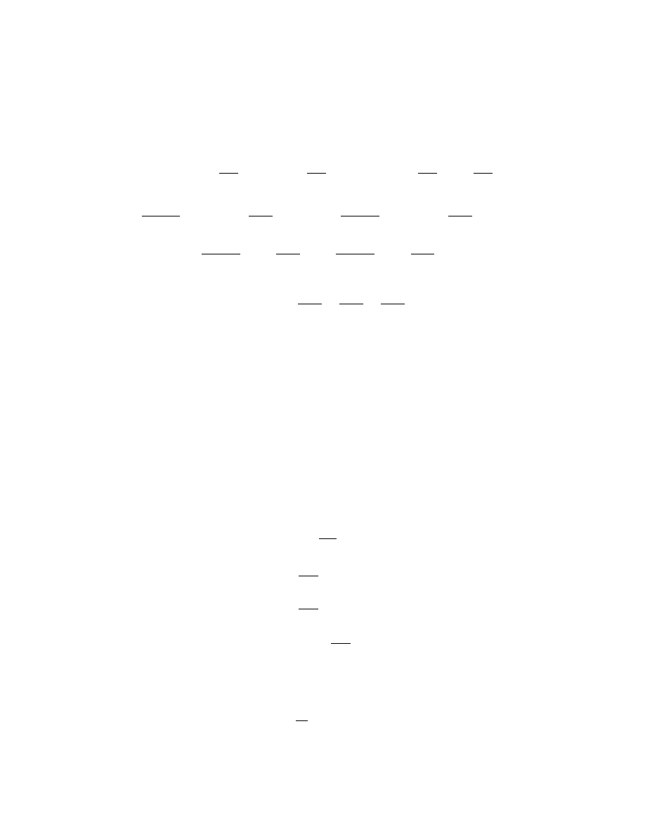
and
d
∗
d(a
1
dx
1
) = d
∗
(
∂a
1
∂x
2
dx
2
∧ dx
1
+
∂a
1
∂x
3
dx
3
∧ dx
1
) = ∗d(
∂a
1
∂x
2
dx
3
−
∂a
1
∂x
3
dx
2
)
= ∗(
∂
2
a
1
∂x
1
∂x
2
dx
1
∧ dx
3
+
∂
2
a
1
∂x
2
2
dx
2
∧ dx
3
−
∂
2
a
1
∂x
1
∂x
3
dx
1
∧ dx
2
−
∂
2
a
1
∂x
2
3
dx
3
∧ dx
2
)
=
∂
2
a
1
∂x
1
∂x
2
dx
2
−
∂
2
a
1
∂x
2
2
dx
1
+
∂
2
a
1
∂x
1
∂x
3
dx
3
−
∂
2
a
1
∂x
2
3
dx
1
.
Adding, we get
∆(a
1
dx
1
) = −
∂
2
a
1
∂x
2
1
+
∂
2
a
1
∂x
2
2
+
∂
2
a
1
∂x
2
3
dx
1
which is the negative of the usual Laplacian on the coefficient a
1
. By linearity the
same is true for a general 1-form a
1
dx
1
+ a
2
dx
2
+ a
3
dx
3
.
When p = 0 we have
∆f = d
∗
df = (−1)
n+n+1
∗ d ∗ df = − ∗ d ∗ df
and this is sometimes called the Laplace-Beltrami operator, though there are differing
conventions about sign:
Example:
1. Take M = R
n
with the Euclidean metric.
df
=
X
i
∂f
∂x
i
dx
i
∗df =
∂f
∂x
1
dx
2
∧ . . . ∧ dx
n
+ . . .
d ∗ df
=
∂
2
f
∂x
2
1
dx
1
∧ dx
2
∧ . . . ∧ dx
n
+ . . .
∆f = − ∗ d ∗ df
= −
X
i
∂
2
f
∂x
2
i
2. Take M to be the upper half-plane with metric
g =
1
y
2
(dx
2
+ dy
2
).
81
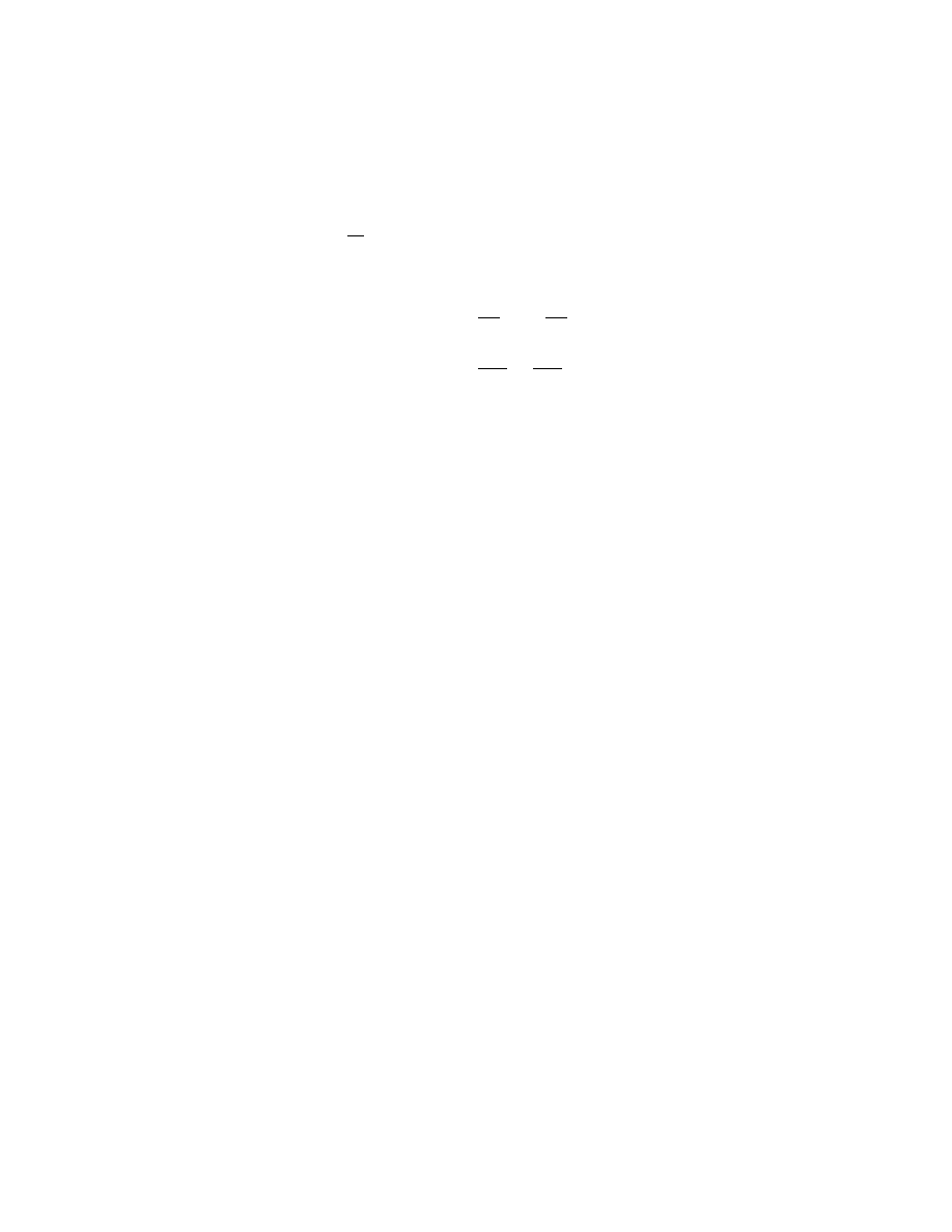
Then
ω =
1
y
2
dx ∧ dy
∗ dx = dy,
∗dy = −dx.
So
∆f
= − ∗ d(
∂f
∂x
dy −
∂f
∂y
dx)
= −y
2
∂
2
f
∂x
2
+
∂
2
f
∂y
2
It follows that the real and imaginary part of a holomorphic function of z = x + iy
satisfy ∆f = 0, just as in the case of the Euclidean metric.
Definition 38 A differential form α ∈ Ω
p
(M ) is a
harmonic form
if ∆α = 0.
On a compact manifold harmonic forms play a very important role, which there is no
time to explore in this course. Here is the starting point:
Proposition 9.5 Let M be a compact oriented Riemannian manifold. Then
• a p-form is harmonic if and only if dα = 0 and d
∗
α = 0
• in each de Rham cohomology class there is at most one harmonic form.
Proof: Clearly if dα = d
∗
α = 0, then (dd
∗
+ d
∗
d)α = 0. Suppose conversely ∆α = 0,
then
0 =
Z
M
(∆α, α)ω =
Z
M
(dd
∗
+ d
∗
d)α, α)ω =
Z
M
(d
∗
α, d
∗
α)ω +
Z
M
(dα, dα)ω.
But these last two terms are non-negative and vanish if and only if dα = d
∗
α = 0.
Suppose α, α
0
are harmonic forms in the same cohomology class, then
α − α
0
= dβ.
But then
0 = d
∗
α − d
∗
α
0
= d
∗
dβ
and
0 =
Z
M
(d
∗
dβ, β)ω =
Z
M
(dβ, dβ)ω
which gives dβ = 0 and α = α
0
.
2
82

The theorem of W.V.D. Hodge says that there exists in each cohomology class a
harmonic form, which as we have seen is unique. This result was a profound influence
on geometry in the last half of the 20th century. The proof is far beyond the scope
of this course, but the interested reader with a week or two to spare can find a proof
in: Foundations of Differentiable manifolds and Lie Groups by F. Warner, Graduate
Texts in Mathematics 94, Springer 1983. There is a natural interpretation of the
result: the harmonic form α in a cohomology class is the one of smallest L
2
norm,
because any other is of the form α + dβ and
Z
M
(α + dβ, α + dβ)ω =
Z
M
(α, α)ω +
Z
M
(dβ, dβ)ω ≥
Z
M
(α, α)ω
since
Z
M
(α, dβ)ω =
Z
M
(d
∗
α, β)ω = 0.
There are some immediate consequences of the Hodge theorem. First note that:
Proposition 9.6 The Laplacian ∆ commutes with ∗.
Proof:
(dd
∗
+ d
∗
d) ∗ α = (−1)
n(n−p)+n+1
d ∗ d ∗ ∗α + (−1)
n(n−p+1)+n+1
∗ d ∗ d ∗ α
= (−1)
n(n−p)+n+1+p(n−p)
d ∗ dα + (−1)
n+pn+1
∗ d ∗ d ∗ α
= (−1)
p+1
d ∗ dα + (−1)
n+pn+1
∗ d ∗ d ∗ α
and
∗(dd
∗
+ d
∗
d)α = (−1)
np+n+1
∗ d ∗ d ∗ α + (−1)
n(p+1)+n+1
d ∗ d ∗ ∗α
= (−1)
np+n+1
∗ d ∗ d ∗ α + (−1)
n(p+1)+n+p(n−p)+1
d ∗ dα
= (−1)
np+n+1
∗ d ∗ d ∗ α + (−1)
p+1
d ∗ dα
2
It follows from the proposition that ∗ maps harmonic forms to harmonic forms. since
∗
2
= (−1)
p(n−p)
it is invertible and so it maps the space of harmonic p-forms isomor-
phically to the space of harmonic n −p forms. One consequence of the Hodge theorem
is that
dim H
p
(M ) = dim H
n−p
(M ).
This we saw for p = 0 rather differently in Theorem 8.2.
83

10
APPENDIX: Technical results
10.1
The inverse function theorem
Lemma 10.1 (Contraction mapping principle) Let M be a complete metric space
and suppose T : M → M is a map such that
d(T x, T y) ≤ kd(x, y)
where k < 1. Then T has a unique fixed point.
Proof: Choose any point x
0
, then
d(T
m
x
0
, T
n
x
0
) ≤ k
m
d(x
0
, T
n−m
x
0
)
for
n ≥ m
≤ k
m
(d(x
0
, T x
0
) + d(T x
0
, T
2
x
0
) + . . . + d(T
n−m−1
x
0
, T
n−m
x
0
))
≤ k
m
(1 + k + . . . + k
n−m−1
)d(x
0
, T x
0
)
≤
k
m
1 − k
d(x
0
, T x
0
)
This is a Cauchy sequence, so completeness of M implies that it converges to x. Thus
x = lim T
n
x
0
and so by continuity of T ,
T x = lim T
n+1
x
0
= x
For uniqueness, if T x = x and T y = y, then
d(x, y) = d(T x, T y) ≤ kd(x, y)
and so k < 1 implies d(x, y) = 0.
2
Theorem 10.2 (Inverse function theorem) Let U ⊆ R
n
be an open set and f :
U → R
n
a C
∞
function such that Df
a
is invertible at a ∈ U . Then there exist
neighbourhoods V, W of a and f (a) respectively such that f (V ) = W and f has a C
∞
inverse on W .
Proof:
By an affine transformation x 7→ Ax + b we can assume that a = 0 and
Df
a
= I. Now consider g(x) = x − f (x). By construction Dg
0
= 0 so by continuity
there exists r > 0 such that if kxk < 2r,
kDg
x
k <
1
2
84
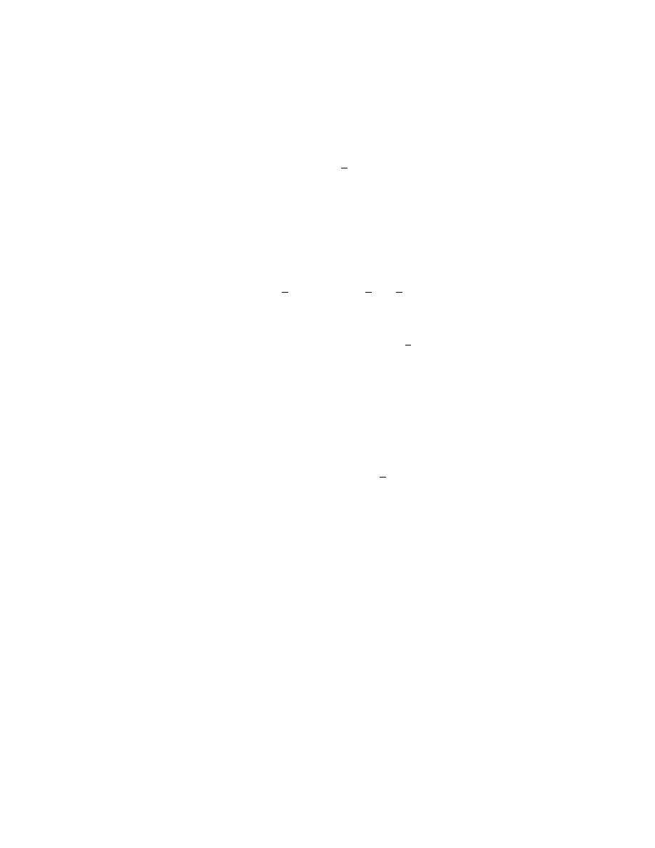
It follows from the mean value theorem that
kg(x)k ≤
1
2
kxk
and so g maps the closed ball ¯
B(0, r) to ¯
B(0, r/2). Now consider
g
y
(x) = y + x − f (x)
(The choice of g
y
is made so that a fixed point g
y
(x) = x solves f (x) = y).
If now kyk ≤ r/2 and kxk ≤ r, then
kg
y
(x)k ≤
1
2
r + kg(x)k ≤
1
2
r +
1
2
r = r
so g
y
maps the complete metric space M = ¯
B(0, r) to itself. Moreover
kg
y
(x
1
) − g
y
(x
2
)k = kg(x
1
) − g(x
2
)k ≤
1
2
kx
1
− x
2
k
if x
1
, x
2
∈ ¯
B(0, r), and so g
y
is a contraction mapping. Applying Lemma 1 we have a
unique fixed point and hence an inverse ϕ = f
−1
.
We need to show first that ϕ is continuous and secondly that it has derivatives of all
orders. From the definition of g and the mean value theorem,
kx
1
− x
2
k ≤ kf (x
1
) − f (x
2
)k + kg(x
1
) − g(x
2
)k
≤ kf (x
1
) − f (x
2
)k +
1
2
kx
1
− x
2
k
so
kx
1
− x
2
k ≤ 2kf (x
1
) − f (x
2
)k
which is continuity for ϕ. It follows also from this inequality that if y
1
= f (x
1
) and
y
2
= f (x
2
) where y
1
, y
2
∈ B(0, r/2) then x
1
, x
2
∈ ¯
B(0, r), and so
kϕ(y
1
) − ϕ(y
2
) − (Df
x
2
)
−1
(y
1
− y
2
)k = kx
1
− x
2
− (Df
x
2
)
−1
(f (x
1
) − f (x
2
))k
≤ k(Df
x
2
)
−1
kkDf
x
2
(x
1
− x
2
) − f (x
1
) + f (x
2
)k
≤ Akx
1
− x
2
kR
where A is a bound on k(Df
x
2
)
−1
k and the function kx
1
− x
2
kR is the remainder
term in the definition of differentiability of f . But kx
1
− x
2
k ≤ 2ky
1
− y
2
k so as
y
1
→ y
2
, x
1
→ x
2
and hence R → 0, so ϕ is differentiable and moreover its derivative
is (Df )
−1
.
Now we know the derivative of ϕ:
Dϕ = (Df )
−1
so we see that it is continuous and has as many derivatives as f itself, so ϕ is C
∞
.
2
85

10.2
Existence of solutions of ordinary differential equations
Lemma 10.3 Let M be a complete metric space and T : M → M a map. If T
n
is
a contraction mapping, then T has a unique fixed point.
Proof:
By the contraction mapping principle, T
n
has a unique fixed point x. We
also have
T
n
(T x) = T
n+1
x = T (T
n
x) = T x
so T x is also a fixed point of T
n
. By uniqueness T x = x.
2
Theorem 10.4 Let f (t, x) be a continuous function on |t − t
0
| ≤ a, kx − x
0
k ≤ b and
suppose f satisfies a Lipschitz condition
kf (t, x
1
) − f (t, x
2
)k ≤ kx
1
− x
2
k.
If M = sup |f (t, x)| and h = min(a, b/M ), then the differential equation
dx
dt
= f (t, x),
x(t
0
) = x
0
has a unique solution for |t − t
0
| ≤ h.
Proof: Let
(T x)(t) = x
0
+
Z
t
t
0
f (s, x(s))ds
Then T x is differentiable since f and x are continuous and if T x = x, x satisfies the
differential equation (differentiate the definition). We use the metric space
X = {x ∈ C([t
0
− h, t
0
+ h], R
n
) : kx(t) − x
0
k ≤ M h}
with the uniform metric
d(x
1
, x
2
) =
sup
|t−t
0
|≤h
kx
1
(t) − x
2
(t)k
which makes it complete. If x ∈ M , then T x ∈ M and we claim
|T
k
x
1
(t) − T
k
x
2
(t)k ≤
c
k
k!
|t − t
0
|
k
d(x
1
, x
2
)
86

For k = 0 this is clear, and in general we use induction to establish:
kT
k
x
1
(t) − T
k
x
2
(t)k ≤
Z
t
t
0
kf (s, T
k−1
x
1
(s) − f (s, T
k−1
x
2
(s)kds
≤ c
Z
t
t
0
kT
k−1
x
1
(s) − T
k−1
x
2
(s)kds
≤ (c
k
/(k − 1)!)
Z
t
t
0
|s − t
0
|
k−1
ds d(x
1
, x
2
)
≤ (c
k
/k!)|t − t
0
|
k
d(x
1
, x
2
)
So T
n
is a contraction mapping for large enough N , and the result follows.
2
Theorem 10.5 The solution above depends continuously on the initial data x
0
.
Proof: Take h
1
≤ h and δ > 0 such that M h + δ ≤ b, and let
Y = {y ∈ C([t
0
− h
1
, t
0
+ h
1
] × ¯
B(x
0
, δ); R
n
: ky(t, x) − xk ≤ M h, y(t
0
, x) = x}
which is a complete metric space as before. Now set
(T y)(t, x) = x +
Z
t
t
0
f (s, y(s, x))ds
Since M h
1
+ δ ≤ b, T maps Y to Y and just as before T
n
is a contraction mapping
with a unique fixed point which satisfies
∂y
∂t
= f (t, y),
y(t
0
, x) = x
Since y is continuous in t and x this is what we need.
2
If f (t, x) is smooth then we need more work to prove that the solution to the equation
is smooth and smoothly dependent on parameters.
10.3
Smooth dependence
Lemma 10.6 Let A(t, x), B(t, x) be continuous matrix-valued functions and take
M ≥ sup
t,x
kBk. The solutions of the linear differential equations
dξ(t, x)
dt
= A(t, x)ξ(t, x),
ξ(t
0
, x) = a(x)
dη(t, x)
dt
= B(t, x)η(t, x),
η(t
0
, x) = b(x)
87

satisfy
sup
x
kξ(t, x) − η(t, x)k ≤ CkA − Bk
e
M |t−t
0
|
− 1
M
+ ka − bke
M |t−t
0
|
where C is a constant depending only on A and a.
Proof:
By the existence theorem we know how to find solutions as limits of ξ
n
, η
n
where
ξ
k
= a +
Z
t
t
0
Aξ
k−1
ds
η
k
= b +
Z
t
t
0
Bη
k−1
ds
Let g
k
(t) = sup
x
kξ
k
(t, x) − η
k
(t, x)k and C = sup
k,x,t
kξ
k
k. Then
g
n
(t) ≤ ka − bk + CkA − Bk|t − t
0
| + M
Z
t
t
0
g
n−1
(s)ds
Now define f
n
by f
0
(t) = ka − bk and then inductively by
f
n
(t) = ka − bk + CkA − Bk|t − t
0
| + M
Z
t
t
0
f
n−1
(s)ds
Comparing these two we see that f
n
≥ g
n
. This is a contraction mapping, so that
f
n
→ f with
f (t) = ka − bk + CkA − Bk|t − t
0
| + M
Z
t
t
0
f (s)ds
and solving the corresponding differential equation we get
f (t) = ka − bke
M |t−t
0
|
+ CkA − Bk
e
M |t−t
0
|
− 1
M
As g
n
(t) ≤ f
n
(t),
sup
x
kξ
n
(t, x) − η
n
(t, x)k ≤ f
n
(t)
and the theorem follows by letting n → ∞.
2
Theorem 10.7 If f is C
k
and
d
dt
α(t, x) = f (t, α(t, x)),
α(0, x) = x
then α is also C
k
.
88

Proof:
The hardest bit is k = 1. Assume f is C
1
so that ∂f /∂t and ∂f /∂x
i
exist
and are continuous. We must show that α is C
1
in all variables. If that were true,
then the matrix valued function λ where (λ
i
= ∂α/∂x
i
) would be the solution of the
differential equation
dλ
dt
= D
x
f (t, α)λ
(25)
so we shall solve this equation by the existence theorem and prove that the solution
is the derivative of α. Let F (s) = f (t, a + s(b − a)). Then
dF
ds
= D
x
f (t, a + s(b − a))(b − a)
so
f (t, b) − f (t, a) =
Z
1
0
D
x
f (t, a + s(b − a))(b − a)ds
But then
d
dt
(α(t, x + y) − α(t, x)) = f (t, α(t, x + y)) − f (t, α(t, x))
=
Z
1
0
D
x
f (t, α(t, x) + s(α(t, x + y) − α(t, x)))(α(t, x + y) − α(t, x))ds
Let A(t, x) = D
x
f (t, α(t, x)) and ξ(t, x) = λ(t, x)y and
B
y
(t, x) =
Z
1
0
D
x
f (t, α(t, x)+s(α(t, x+y)−α(t, x)))ds,
η
y
(t, x) = α(t, x+y)−α(t, x)
Apply the previous lemma and we get
sup
|t|≤
kλ(t, x)y − (α(t, x + y) − α(x))k = o(ky|)
and so D
x
α = λ, which is continuous in (t, x). Since also dα/dt = f (t, α) this means
that α is C
1
in all variables.
To continue, suppose inductively that the theorem is true for k − 1, and f is C
k
.
Then A(t, x) = D
x
f (t, α(t, x)) is C
k−1
but since
dλ
dt
= Aλ
we have λ is C
k−1
. Now D
x
α = λ so the x
i
-derivatives of α are C
k−1
. But also
dα/dt = f (t, α) is C
k−1
too, so α is C
k
.
2
89

10.4
Partitions of unity on general manifolds
Definition 39 A partition of unity on M is a collection {ϕ
i
}
i∈I
of smooth functions
such that
• ϕ
i
≥ 0
• {supp ϕ
i
: i ∈ I} is locally finite
•
P
i
ϕ
i
= 1
Here locally finite means that for each x ∈ M there is a neighbourhood U which
intersects only finitely many supports supp ϕ
i
.
Theorem 10.8 Given any open covering {V
α
} of M there exists a partition of unity
{ϕ
i
} on M such that supp ϕ
i
⊂ V
α(i)
for some α(i).
Proof: (by exhaustion – !)
1. M is locally compact since each x ∈ M has a neighbourhood homeomorphic to,
say, the open unit ball in R
n
. So take U homeomorphic to a smaller ball, then ¯
U
is compact. Since M is Hausdorff, ¯
U is closed (compact implies closed in Hausdorff
spaces).
2. M has a countable basis of open sets {U
j
}
j∈N
, so x ∈ U
j
⊂ U and ¯
U
j
⊂ ¯
U is
compact so M has a countable basis of open sets with ¯
U
j
compact.
3. Put G
1
= U
1
. Then
¯
G
1
⊂
∞
[
j=1
U
j
so by compactness there is k > 1 such that
¯
G
1
⊂
k
[
j=1
U
j
= G
2
Now take the closure of G
2
and do the same. We get compact sets ¯
G
j
with
¯
G
j
⊂ G
j+1
M =
∞
[
j=1
U
j
90

4. By construction we have
¯
G
j
\G
j−1
⊂ G
j+1
\ ¯
G
j−2
and the set on the left is compact and the one on the right open. Now take the given
open covering {V
α
}. The sets V
α
∩ (G
j+1
\ ¯
G
j−2
) cover ¯
G
j
\G
j−1
. This latter set is
compact so take a finite subcovering, and then proceed replacing j with j + 1. This
process gives a countable locally finite refinement of {V
α
}, i.e. each V
α
∩ (G
j+1
\ ¯
G
j−2
)
is an open subset of V
α
. It is locally finite because
G
j+1
\ ¯
G
j−2
∩ G
j+4
\ ¯
G
j+1
= ∅
5. For each x ∈ M let j be the largest natural number such that x ∈ M \ ¯
G
j
. Then
x ∈ V
α
∩ (G
j+2
\ ¯
G
j−1
). Take a coordinate system within this open set and a bump
function f which is identically 1 in a neighbourhood W
x
of x.
6. The W
x
cover ¯
G
j+1
\G
j
and so as x ranges over the points of G
j+2
\ ¯
G
j−1
we get
an open covering and so by compactness can extract a finite subcovering. Do this
for each j and we get a countable collection of smooth functions ψ
i
such that ψ
i
≥ 0
and, since the set of supports is locally finite,
ψ =
X
ψ
i
is well-defined as a smooth function on M . Moreover
supp ψ
i
⊂ V
α
∩ (G
m
\ ¯
G
m−3
) ⊂ V
α
so each support is contained in a V
α
. Finally define
ϕ
i
=
ψ
i
ψ
then this is the required partition of unity.
2
10.5
Sard’s theorem (special case)
Theorem 10.9 Let M and N be differentiable manifolds of the same dimension n
and suppose F : M → N is a smooth map. Then the set of critical values of F has
measure zero in N . In particular, every smooth map F has at least one regular value.
91

Proof:
Since a countable union of null sets (=sets of measure zero) is null, and M
and N have a countable basis of open sets, it suffices to consider the local case of
F : U → R
n
. Moreover since U is a countable union of compact cubes we need only
prove that the image of the set of critical points in the compact cube K = {x ∈ R
n
:
|x
i
| ≤ 1} is of measure zero.
Now suppose a ∈ K is a critical point, so that the image of DF
a
is contained in a
proper subspace of R
n
, and so is annihilated by a linear form f . Let H ⊂ R
n
be the
hyperplane f (x − F (a)) = 0. Then
d(F (x), H) ≤ kF (x) − (F (a) + DF
a
(x − a))k
(26)
On the other hand since F is C
∞
, from Taylor’s theorem we have a constant C such
that
kF (x) − F (y) − DF
y
(x − y)k ≤ Ckx − yk
2
for all x, y ∈ K, since K is compact. Substituting in (26) this yields
d(F (x), H) ≤ Ckx − ak
2
If kx − ak ≤ η, then d(F (x), H) ≤ Cη
2
. Let M = sup{kDF
x
k : x ∈ K}, then by the
mean value theorem
kF (x) − F (a)k ≤ M kx − ak
for x, a ∈ K and so d(F (x), F (a)) ≤ M η. Thus F (x) lies in the intersection of a slab
of thickness 2Cη
2
around H and a ball of radius M η centred on F (a). Putting the
ball in a cube of side 2M η, the volume of this intersection is less than
2Cη
2
(2M η)
n−1
= 2
n
CM
n−1
η
n+1
Now subdivide the cube into N
n
cubes of side 1/N , and repeat the argument for each
cube. Since now kx − yk ≤
√
n/N , critical points in this cube lie in a volume less
than
2
n
CM
n−1
√n
N
n+1
Since there are at most N
n
such volumes, the total is less than
2
n
M
n−1
Cn
(n+1)/2
N
−1
which tends to zero as N → ∞.
Thus the set of critical values is of measure zero.
2
92
Document Outline
Wyszukiwarka
Podobne podstrony:
Lugo G Differential geometry and physics (lecture notes, web draft, 2006)(61s) MDdg
Gudmundsson S An introduction to Riemannian geometry(web draft, 2006)(94s) MDdg
Athanassopoulos K Notes on symplectic geometry (Univ of Crete, web draft, 2007)(66s) MDdg
Skoruppa N P Funktionentheorie 2 (skript, web draft, 2003)(de)(102s) MCc
Dahl M A brief introduction to Finsler geometry (web draft, 2006)(39s) MDdg (1)
tom Dieck T Differential manifolds (draft, 2009)(O)(80s) MDdg
Gardner Differential geometry and relativity (lecture notes, web draft, 2004) (198s) PGr
Neumann W D Notes on geometry and 3 manifolds, with appendices by P Norbury (web draft, 2004)(54s)
Math Differential Geometry Tensor Analysis In Differentiable Manifolds
Freitag Several complex variables local theory (lecture notes, web draft, 2001)(74s) MCc
Walet N Mathematics for Physicists (web draft, 2002)(81s) MCet
Bobenko A Compact Riemann surfaces (web draft, 2010)(86s) MCc
Dynkin E B Superdiffusions and Positive Solutions of Nonlinear PDEs (web draft,2005)(108s) MCde
Amendola L Dark energy (Heidelberg lectures, web draft, 2005)(43s) PGrc
Novikov S P Solitons and geometry (Lezioni Fermiane, Cambridge Univ Press, 1994, web draft, 1993)(50
Rajeev S G Advanced classical mechanics chaos (Rochester lecture notes, web draft, 2002)(100s) PCtm
Gray R M Toeplitz and circulant matrices a review (web draft, 2005)(89s) MAl
Reid H Solved problems from Peskin Schroeder QFT, chapters 2 to 5 (web draft, 2002)(40s) PQft
Field M , Nicol M Ergodic theory of equivariant diffeomorphisms (web draft, 2004)(94s) PD
więcej podobnych podstron