The Goertzel algorithm is derived from the Discrete Fourier Transform (DFT) and exploits the

periodicity of the phase factor

N

k

j

e

π

2

−

to reduce the computational complexity associated with the DFT

as the Fast Fourier Transform (FFT) does. However the Goertzel algorithm is more efficient than the
FFT, when only a few samples of the DFT are required. With the Goertzel algorithm only 16 samples
of the DFT are required. The Goertzel algorithm can be derived as follows using the DFT equation.

( )

( )

( )

)

1

(

;

2

1

0

2

2

1

0

2

=

=

=

∑

∑

−

=

−

−

=

−

N

kN

j

N

n

N

kn

j

N

kN

j

N

n

N

kn

j

e

e

n

x

e

e

n

x

k

X

π

π

π

π

[1]

( )

k

X

can be written as:

( )

( ) (

)

∑

−

=

−

=

1

0

N

n

k

n

N

h

n

x

k

X

where:

(

)

(

)

N

n

N

k

j

k

e

n

N

h

−

−

=

−

π

2

.

( )

k

X

can now be identified as an output of a filter at

N

m

=

and the filter can be written as follows:

( )

( ) (

)

∑

−

=

−

=

1

0

N

n

k

k

n

m

h

n

x

m

y

.

[2]

Therefore:

( )

( )

N

m

k

k

m

y

N

X

=

=

[3]

This can be read as: the Discrete Fourier Transform

( )

N

X

k

is the output of the filter

( )

m

y

k

at

N

m

=

.

The z-transform of

k

y

,

( )

z

y

k

is given by:

( )

( )

1

2

1

−

−

=

z

e

z

X

z

y

N

k

j

k

π

.

[4]

Deriving the difference equation,

( ) ( )

(

)

( )

0

1

;

1

2

=

−

−

+

=

k

k

N

k

j

k

y

n

y

e

n

x

n

y

π

.

[5]

This can be implemented as a single pole IIR filter as shown in Figure 8.2.

z

-1

+

x(n)

y(n)

N

k

j

e

π

2

Figure 8.2 Structure of a Single Pole Resonator for computing the DFT

Equation [5] involves multiplication by a complex number and each complex multiplication results in
four real multiplications and four real additions.

To avoid complex multiplication, Equation [4] is multiplied by a complex conjugate pole and simplified
as follows:

( )

( )

( )

(

)

(

)

(

)

(

)

( )

]

6

[

.

2

cos

2

1

1

sin

cos

1

sin

cos

1

1

1

1

1

2

1

1

2

1

1

1

2

1

2

1

2

1

2

−

−

−

−

−

−

−

−

−

−

−

−

−

+













−









−

=

−

−

+

−









−

=









−









−











−

=

z

z

k

N

z

e

z

X

j

z

j

z

z

e

z

X

z

e

z

e

z

e

z

X

z

y

k

N

j

k

N

j

k

N

j

k

N

j

k

N

j

k

π

θ

θ

θ

θ

π

π

π

π

π

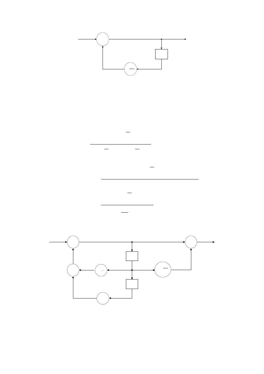
Equation [6] can be implemented using the structure shown in Figure 8.3.

+

+

+

-1

1

−

z

1

−

z

)

( n

y

)

( n

x

k

N

j

e

π

2

−

−













k

N

π

2

cos

2

2

−

n

Q

n

Q

1

−

n

Q

Figure 8.3 Structure of a two Pole Resonator for Computing the k

th

DFT sample

where

( )

2

1

2

cos

2

−

−

−













+

=

n

n

n

Q

Q

N

k

n

x

Q

π

[7]

and

( )

k

N

j

n

n

k

e

Q

Q

n

y

π

2

1

−

−

−

=

[8]

or

( )

( )

N

m

k

k

m

y

N

X

=

=

.

This means that

( )

n

y

k

need not be calculated for every value of m as it only needs to be calculated

at

N

m

=

.

Finally Equations [7] and [8] can be rewritten as follows:

( )

N

n

Q

Q

N

k

n

x

Q

n

n

n

≤

≤

−













+

=

−

−

0

;

2

cos

2

2

1

π

[9]

and

( )

( )

N

n

e

Q

Q

k

X

n

y

k

N

j

N

N

N

n

k

=

−

=

=

−

−

=

;

2

1

π

.

[10]

With this modified structure there is only one complex multiplication for the calculation of each

( )

k

X

.

To implement this algorithm the feedback stage has to be repeated N times and the feedforward stage
to be done once only. Since with DTMF detection we are not interested in the phase information, the
Goertzel algorithm maybe modified to produce an output which is proportional to the magnitude of the
signal. This has the advantage of using only real coefficients and minimising processing time as
shown below.

( )

[

]

,

sin

cos

1

2

θ

θ

θ

π

jB

B

A

Be

A

Q

e

Q

N

y

j

N

k

N

j

N

k

+

−

=

−

=

−

=

−

−

−

where:

n

Q

A

=

1

−

=

n

Q

B

N

k

π

θ

2

=

.

The square of the magnitude is:

( ) (

) (

)

θ

θ

θ

θ

θ

θ

cos

2

sin

cos

cos

2

sin

cos

2

2

2

2

2

2

2

2

2

2

AB

B

A

B

B

AB

A

B

B

A

n

y

k

−

+

=

+

+

−

=

+

−

=

Therefore:

( )

( )

( )

(

)

( ) (

)

1

2

cos

2

1

2

2

2

2

−













−

−

+

=

=

N

Q

N

Q

N

k

N

Q

N

Q

k

X

N

y

k

π

.

[11]

Equation [11] shows that the calculation of

( )

2

k

X

requires only real additions and multiplications.