
Technology Brief
April 1999
0052-0499-A
Prepared by Workstation
Marketing
Compaq Computer Corporation
Contents
Introduction to Graphics
Performance ...............................3
Appearance, Performance
and Price ..................................3
Graphics Concepts ....................4
Computer Graphics and
Performance ...............................5
Geometry Calculations..............5
Rendering.................................6
Pixel Level Operations ..............6
Rendering Performance ............7
Depth Complexity .....................7
How It Looks.............................7
Graphics Performance
Measurements..........................10
Hardware Specifications..........10
Graphics Benchmarks.............11
Application Benchmarks..........11
Benchmark Biases ..................12
Using Graphics Performance
Information ...............................12
Appendix 1:
ViewPerf
Benchmark
14
ProCDRS ...............................14
CDRS.....................................15
DRV .......................................16
DX..........................................17
LIGHT ....................................18
AWADVS................................19
Appendix 2:
Indy3D
Benchmark
21
Overview ................................21
Unique features of Indy3D:......22
Methodology in general...........22
MCAD benchmark ..................22
Animation ...............................23
Simulation ..............................24
Image Quality test...................24
Primitive Tests ........................25
Appendix 3:
The
Graphics Pipeline .....................27
Appendix 4:
Additional
Resources
29
Graphics Performance:
Measures, Metrics and Meaning
Abstract: Graphics performance is a key component of total
systems performance in many applications. Thus, graphics
performance is a critical factor in choosing and configuring
workstations. 3D graphics is widely used in technical applications,
and has undergone dramatic growth in performance and capabilities
over the past few years, while dropping in price to the point where it
is a standard part of even entry level workstations.
Many of the new graphics capabilities, such as texture mapping, are
unfamiliar. In addition, there are several different ways to measure
graphics performance, and many different ways to design computer
systems. Emphasis on different aspects of workstation design by
various vendors can make direct comparisons difficult.
This paper is intended to provide an introduction to 3D computer
graphics concepts and functions, to explain the different ways to
measure graphics performance, and to provide insight into
understanding and using graphics performance measurements and
graphics benchmarks.
Also included is a bibliography of sources for more information and
pointers to on-line sources for the latest performance data.

Graphics Performance: Measures, Metrics and Meaning
2
0052-0499-A
Notice
The information in this publication is subject to change without notice and is provided “AS IS” WITHOUT
WARRANTY OF ANY KIND. THE ENTIRE RISK ARISING OUT OF THE USE OF THIS
INFORMATION REMAINS WITH RECIPIENT. IN NO EVENT SHALL COMPAQ BE LIABLE FOR
ANY DIRECT, CONSEQUENTIAL, INCIDENTAL, SPECIAL, PUNITIVE OR OTHER DAMAGES
WHATSOEVER (INCLUDING WITHOUT LIMITATION, DAMAGES FOR LOSS OF BUSINESS
PROFITS, BUSINESS INTERRUPTION OR LOSS OF BUSINESS INFORMATION), EVEN IF
COMPAQ HAS BEEN ADVISED OF THE POSSIBILITY OF SUCH DAMAGES.
The limited warranties for Compaq products are exclusively set forth in the documentation accompanying
such products. Nothing herein should be construed as constituting a further or additional warranty.
This publication does not constitute an endorsement of the product or products that were tested. The
configuration or configurations tested or described may or may not be the only available solution. This test
is not a determination or product quality or correctness, nor does it ensure compliance with any federal
state or local requirements.
Product names mentioned herein may be trademarks and/or registered trademarks of their respective
companies.
Compaq, Contura, Deskpro, Fastart, Compaq Insight Manager, LTE, PageMarq, Systempro, Systempro/LT,
ProLiant, TwinTray, ROMPaq, LicensePaq, QVision, SLT, ProLinea, SmartStart, NetFlex, DirectPlus,
QuickFind, RemotePaq, BackPaq, TechPaq, SpeedPaq, QuickBack, PaqFax, Presario, SilentCool,
CompaqCare (design), Aero, SmartStation, MiniStation, and PaqRap, registered United States Patent and
Trademark Office.
Netelligent, Armada, Cruiser, Concerto, QuickChoice, ProSignia, Systempro/XL, Net1, LTE Elite,
Vocalyst, PageMate, SoftPaq, FirstPaq, SolutionPaq, EasyPoint, EZ Help, MaxLight, MultiLock,
QuickBlank, QuickLock, UltraView, Innovate logo, Wonder Tools logo in black/white and color, and
Compaq PC Card Solution logo are trademarks and/or service marks of Compaq Computer Corporation.
Microsoft, Windows, Windows NT, Windows NT Server and Workstation, Microsoft SQL Server for
Windows NT are trademarks and/or registered trademarks of Microsoft Corporation.
NetWare and Novell are registered trademarks and intraNetWare, NDS, and Novell Directory Services are
trademarks of Novell, Inc.
Pentium is a registered trademark of Intel Corporation.
Copyright ©1999 Compaq Computer Corporation. All rights reserved. Printed in the U.S.A.
Graphics Performance: Measures, Metrics and Meaning
Technology Brief prepared by Workstation Marketing
First Edition (April 1999)
Document Number 0052-0499-A

Graphics Performance: Measures, Metrics and Meaning
3
0052-0499-A
Introduction to Graphics Performance
Graphics performance is a key component of total systems performance in many applications.
Thus, graphics performance is a critical element in choosing and configuring workstations. 3D
graphics is widely used in technical applications, and has undergone dramatic growth in
performance and capabilities over the past few years, while dropping in price to the point where it
is a standard part of even entry level workstations.
Many of the new graphics capabilities, such as texture mapping, are unfamiliar. There are several
different ways to measure graphics performance, and many different ways to design computer
systems. Emphasis on different aspects of workstation design by various vendors can make direct
comparisons difficult.
This paper is intended to provide an introduction to 3D computer graphics concepts and
functions, to explain the different ways to measure graphics performance, and to provide insight
into understanding and using graphics performance measurements.
Also included is a bibliography of sources for more information and pointers to on-line sources
for the latest performance data.
Appearance, Performance and Price
Traditional discussions of computer graphics center on graphics hardware and performance
specifications for this hardware. We will take a different approach and look at graphics issues
from an application perspective and a user perspective. We will then bring these points of view
together and examine how they impact graphics hardware and the overall system.
The three major variables in computer graphics are appearance (image quality), performance and
price. All systems involve tradeoffs between these factors, and continuing development of
graphics hardware and systems keeps changing the ground rules. For example, a traditional
bottleneck of 3D graphics has been hardware rendering performance. Today, application
performance is a common limiting factor.
We begin by looking at graphics from an application perspective. For 3D graphics, OpenGL has
been a major breakthrough. OpenGL provides a common set of graphics functions and
capabilities. In a base implementation, with a simple frame buffer, all of the 3D functions are
implemented in software. Any image that can be created by an ultra high end 3D graphics
accelerator can be created using pure software OpenGL. Full 3D shading, z-buffering, texturing,
advanced lighting, alpha blending, and other advanced features is available on all OpenGL
systems.
Some capabilities, most notably resolution and color depth, are still determined by the graphics
hardware. But in general, the reason for using 3D graphics hardware is performance. The right
3D graphics hardware can literally change performance from 30 seconds per frame to 30 frames
per second!
The tradeoff is price. In general, the more graphics capabilities accelerated by hardware – and the
greater the acceleration – the more the graphics subsystem will cost. The highest performance
graphics systems will implement all features in hardware. These systems, commonly used in high
end flight simulators, handle massive databases, complex models, high resolution displays, and
deliver a guaranteed update rate of 60 frames per second. These systems may easily cost $1
million or more.

Graphics Performance: Measures, Metrics and Meaning
4
0052-0499-A
The revolution that has occurred over the past few years is the availability of relatively high
performance 3D graphics (currently exceeding 4 million triangles/second) in a under $2,000
graphics system. Today’s systems deliver good performance, good resolution, and good feature
sets at an attractive price.
The key to a successful system is a balanced system where all of the components -- including
graphics -- work together, and no components are dramatically faster or slower than the others.
This paper provides a background for understanding graphics and graphics performance in the
context of an overall system. We will explore graphics concepts, hardware and software
implementation issues, graphics performance and performance measurement, and conclude with
an overview of two of the most popular 3D graphics benchmarks -- ViewPerf and Indy3D.
Graphics Concepts
Computer graphics is the process of turning abstract information into glowing dots on a computer
monitor. Although the end result is the same in all cases, special processing is required for
different types of abstract information. At the highest level, the abstract information represents
the data for a specific application, and varies from application to application. The application
produces graphics commands, which are commonly described as 2D or 3D. These graphics
commands are then processed by the workstation graphics system to produce images on the
computer screen.
A fundamental characteristic of computer screens is that they are flat – they are two dimensional.
This means that 2D information can be displayed with minimal processing – there is a good
match between the graphics data and the display.
3D information is radically different than 2D information, and can not be directly displayed on a
2D screen. Additional processing is needed to produce a specific 2D view from the 3D data.
Further, new capabilities arise with 3D data – like real world physical objects, a 3D surface can
be illuminated with light, can be opaque or transparent, can have color and surface patterns, and
can include a variety of objects that are in front of and behind each other – and even moving
around!
3D graphics is used to convey information. This can include abstract information, such as
pressure, temperature, and flow direction in a computational fluid dynamics analysis; 3D surface
representations, as in the design of mechanical parts in a CAD system; or a realistic
representation of the real world, as in flight simulators and virtual reality systems.
These differing types of information are represented with different graphics entities. 2D graphics
uses 2D vectors (line segments with a start point and end point), 2D areas (filled shapes on the
screen), and raster data (arrays of data corresponding to the pixels on the screen). 3D graphics
uses 3D vectors and 3D surfaces. To simplify processing and improve performance, curved 3D
surfaces are commonly broken down into a collection of small flat polygons, usually three sided
(triangles) or four sided (quadrilaterals). The most common is the triangle, which can be
efficiently displayed and shaded.
An interesting point is that virtually all “3D” graphics is actually a combination of 2D and 3D
graphics –windows, text, tables, graphics, users interfaces and similar data are 2D. To achieve
good performance running applications, a workstation must provide high performance on both 2D
and 3D graphics – and on the combination of 2D and 3D graphics together! User interfaces
provide special challenges, with their tendency to dynamically appear over the top of other
graphics, and then quickly disappear.

Graphics Performance: Measures, Metrics and Meaning
5
0052-0499-A
Advanced hardware capabilities such as overlay planes, stencil planes, fast clear planes and blt
engines are necessary to support high performance in this mixed 2D/3D environment.
Computer Graphics and Performance
In any discussion of computer graphics, the first question has to be “where do the graphics come
from?” In any interesting case, graphics commands are produced by an application. The phrase
"interesting case" is used to distinguish applications -- which do useful work -- from benchmarks.
Benchmarks are informative, but applications are truly important. To somewhat simplify our
discussion, an application produces graphics commands and graphics primitives, which are then
processed through the graphics system.
Thus, the first question in graphics performance is “how fast can the application produce graphics
commands?” This is the first critical bottleneck. If the graphics system can process graphics
commands as fast as or faster than the application can produce them, then a faster graphics
system will not improve graphics performance!
This somewhat surprising result drives home the prime rule of computer performance – total
system performance is gated by the performance of the slowest component of the system. The
implication is that improvements in system performance are achieved by improving the
performance of the slowest component – the weakest link in the performance chain. Improving
the performance of other parts of the system will tend to have minimal impact on system
performance.
Assuming that the application is “fast enough” – and this assumption should always be checked--
the graphics subsystem should then be examined.
3D graphics can be broken down into two major pieces – geometry and rendering. Geometry
consists of transformations, lighting calculations, texturing calculations, culling, and similar
operations. Geometry primarily involves calculations – mainly floating point computations – on
the vertices of geometric primitives. The main geometric primitives used are lines and triangles.
Rendering consists of taking the results of the geometry calculations and further processing them
to produce individual pixels on the screen. Geometry calculations are typically done in the host
processor or a dedicated geometry engine. Rendering is typically done in the graphics hardware.
Geometry and rendering each have unique requirements and characteristics.
A brief overview of geometry and rendering is provided here – see Appendix 3 for more detail on
the graphics pipeline.
Geometry Calculations
Geometry calculations consist of computations done on vertices (3D points) to transform, light,
clip, cull, and texture. The major characteristics are extensive floating point computations, the
movement of large amounts of data, and the application of complex algorithms. As such, key
performance measures include floating point performance (measured in MFLOPS), data
movement (measured in Mbytes/sec), and the ability to execute OpenGL algorithms (measured in
“does it work”).
Another aspect of this is efficiency – how effectively can the graphics system process the
geometry. Key elements include pipelining, parallelism, and latency in performing the required
calculations, register utilization and cache hit rate in manipulating instructions and data, and
memory bandwidth. As can readily be seen, hardware peak performance numbers are not a good
indicator of geometry processing power. The only effective way to determine actual geometry

Graphics Performance: Measures, Metrics and Meaning
6
0052-0499-A
performance is to measure it running graphics. This is where graphics benchmarks are extremely
valuable for measuring performance.
After geometric calculations are completed, the final lines and triangles are rendered.
Rendering
Rendering takes geometry and processes it to "fill in" the inside of the polygon. This is done by
producing the pixels inside the polygon through a process called interpolation. There are two
components to this process: setup and fill.
Setup takes the vertex data, loads it into registers in the graphics hardware, performs a set of
calculations called slope generation and starts the fill process. The setup phase determines the
geometry limit, measured in triangles per second, that the graphics hardware can achieve.
Once setup is completed, the line is drawn or the triangle is filled. This operation produces the
individual pixels that are displayed. This fill rate is measured in pixels per second. The common
units for measuring this is Mpixels – millions of pixels per second.
Pixel Level Operations
After a pixel is generated, a set of pixel level computations are done to determine if the pixel is
actually drawn. These include window clipping, Z-buffering, window ID, and alpha blending.
Window clipping checks to see if the pixel is inside or outside of the window it is being drawn to.
This occurs when a triangle is partially outside of the window. If the pixel is outside of the
window boundary, it is discarded. If it is inside the window boundary, it is drawn. For good
performance, window clipping should be done in hardware.
Z buffering is a technique used to draw only the pixel that is in front of others. Each pixel has an
XY screen location, and also has a Z or depth value which measures how far it is from the eye
point. When a pixel is drawn, the Z value for that location is read first. If the new pixel is closer
to the eye point than the existing pixel, then the new pixel is drawn and the Z value is updated. If
the new pixel is farther from the eye point than the existing pixel, than the new pixel is discarded
and the original pixel is left unmodified.
Alpha blending is used to handle partially transparent objects. Normally, an object is either
completely opaque or completely transparent. With alpha blending, the object is assigned an
opacity value, typically 0-255, where 0 is totally transparent and 255 is completely opaque.
Alpha blending is combined with Z buffering: If the new pixel is behind the existing pixel, it is
discarded. If the new pixel is in front of the old pixel, then a hybrid pixel is produced by
combining the new and old pixels, with the ratio between new and old pixels determined by the
new pixels alpha value.
The Window ID is used to determine if the pixel is in the active window. In modern windowing
systems, including Xwindows and Win32, it is possible to have multiple windows stacked on top
of each other – or even worse, partially on top of each other. Only the top window is actually
drawn, so it is necessary to check for each pixel whether or not it is in the topmost window. For
best performance, the Window ID for the topmost window is stored with each pixel on the screen.
When a pixel is to be drawn, the graphics system checks to see if it is in the topmost window. If
so, it is drawn. If it is not in the topmost window, then the pixel is discarded.

Graphics Performance: Measures, Metrics and Meaning
7
0052-0499-A
Rendering Performance
As there are two distinct components to rendering, either one can be the performance bottleneck.
We will explore this with a specific example: Assume that we have a graphics board that has a
setup rate of one million triangles per second and a fill rate of 50 Mpixels.
If we have an average triangle size of 25 pixels, we will achieve a maximum performance of 1M
triangles/sec. In this case, the hardware has enough pixel fill capacity to fill 2M 25 pixel
triangles, but is gated by the setup rate.
If we have an average triangle size of 100 pixels, we will achieve a maximum performance of
500K triangles/sec. In this case, the hardware can process 1M triangles/sec, but is gated by fill
rate.
Depending on triangle size, either setup or fill might dominate. If the average triangle is small
(common in CAD and Scientific Visualization applications), then setup rate is the most important
factor. If the average triangle is large (common in visual simulation applications), then fill rate is
the most important factor.
Depth Complexity
A commonly overlooked factor that can have a major impact on perceived graphics performance
is depth complexity. Assume that you have a thousand triangle, all stacked on top of each other.
When this data is drawn, the system will process all thousand triangles, but only one will be
visible.
While stacking objects a thousand deep is somewhat extreme, it is quite common to have objects
stacked two, three, or four deep. If a scene has an average depth complexity of two, then each
pixel on the screen will be drawn an average of two times. The result of this is graphics
performance that is half of what might be expected based on the number of pixels being
displayed.
How It Looks
Several factors impact both the appearance of an image on the screen as well as graphics
performance. These include color depth, double buffering, resolution and anti-aliasing. A
special case is stereo viewing.
Color Depth
Color depth is the number of colors that can be displayed, and is measured in number of bits or
color planes. A color plane is a one-bit buffer covering the screen. A single plane can represent
black and white, and is used in older systems. Multiple bit planes are stacked on top of each
other, and used to represent color or multiple level gray-scale data. Common color depths are 8
bit, 12 bit, 16 bit and 24 bit. 24 bit color is often called true color.
The collection of color planes used to display an image is called the frame buffer.
Color can be used two ways: directly, or through a lookup table. To explain the difference, we
need to briefly consider what color is. Computer displays work in terms of three primary colors:
red, green, and blue. Color monitors and flat panel displays contain an array of tiny red, green
and blue dots. Each dot can be individually turned on and off. In addition, each dot can be set at
different levels of brightness. Typically, each dot will have 256 levels of brightness, requiring 8

Graphics Performance: Measures, Metrics and Meaning
8
0052-0499-A
bits of data to set. A set of three dots, one red, one green, and one blue, are combined to make a
single pixel. By combining the red, green, and blue, the pixel can display any color.
8 bits per color combined with the three primary colors produces 24 bits of color information.
This is convenient for computer use for several reasons. First, 256 levels of brightness is a good
fit for monitors – it can be readily achieved, yet significantly more levels would be difficult to
achieve with current technology. Second, 8 bits of data (a byte), is a natural unit of information
for computers to work with. Third, 24 bits provides 16.7 million colors, allowing a natural
representation. 16.7 million colors is a good match for the range of color a monitor can display
and that the human eye can perceive. Significantly fewer bits of information produces highly
noticeable banding and other undesirable artifacts. Significantly more bits of information
provides finer changes that can’t be seen. Thus, 24 bit color is the optimum color depth for most
computer graphics.
As a side note, there are some cases where greater color depth is used. High end animation will
often render with 30 or 36 bit data (10 or 12 bits per color). The renderings are output on 35mm
film with special recorders that can reproduce that color depth. Likewise, photographic images
for high end color printing will often be scanned in and manipulated in 30 bit or 36 bit format.
8 bit color allows the display of 256 colors. To improve visual quality, a table with 256 entries is
used. Each entry contains a 24 bit color value. This table is called a color palette or color lookup
table, and contains all of the colors that can be displayed. The color lookup table is maintained in
the graphics hardware. The system (or application) will determine the color value entered in
each entry in the color lookup table. Thus, any color can be displayed, but only 256 colors can be
used at a time.
A single color lookup table can be used for the entire display or for a single window. Windows
NT uses a single table for the entire display. A side effect of this approach is the often dramatic
color changes seen when an application changes a color lookup table used by other applications.
X-Windows allows a separate color lookup table to be used for each window, which avoids these
color changes. A common implementation for X-Windows is to use four color lookup tables.
The other approach is to allow direct manipulation of the color. Using this approach, the
application will directly control the red, green, and blue color data, and will directly set the levels
for each color. This is a strong advantage for 3D applications, since they calculate direct color
values.
Direct color is commonly implemented with 12, 16 or 24 bits. 12 bit and 16 bit require less frame
buffer memory, thus (at least theoretically) reducing cost. However, 12 bit is implemented with
only 4 bits per color (16 levels), and 16 bit with 5 bits per color (32 levels). This produces strong
banding and other artifacts in the display, resulting in a poor quality image.
For 3D graphics, 24 bit true color should be considered a mandatory requirement.
Double Buffering
Double buffering is a technique used to improve display quality by making changes in the image
appear smoother.
Recall that a frame buffer contains the image that is displayed on the screen. When the image is
updated, the frame buffer is cleared (set to solid black), and then the new image is drawn. This
process is usually visible. With a fast system, it may be noticeable as a flicker when the frame
buffer is cleared and redrawn. With a slower system, it may be possible to actually seen the
image being drawn.

Graphics Performance: Measures, Metrics and Meaning
9
0052-0499-A
To avoid this, two frame buffers are used: a display frame buffer (often called the front buffer),
and a working frame buffer (often called the back buffer). All drawing operations are done to the
back buffer. When the drawing operations are completed, the back buffer is swapped with the
front buffer (an essentially instantaneous operation). Then, the back buffer is cleared and the next
image is drawn.
The result of this process is that the system appears to move smoothly. The visible difference to a
user is dramatic, so much so that single buffered graphics should not be considered for serious 3D
systems.
A double buffered true color display should be considered a pre-requisite for workstation class
3D graphics.
Resolution
Resolution is the number of pixels that are displayed. It is measured in number of pixels
horizontally and vertically – for example, 1280x1024. Resolution has a major influence on
display quality and on the amount of detail that can be seen. In general, the higher the resolution,
the better the image quality.
Resolution is one of the graphics differences between workstations and personal computers. In
general, 1280x1024 is the minimum resolution for workstation class graphics. Higher resolutions
are often used, with 1600x1200 being a common choice.
While high resolution improves appearance, it hurts performance. This is because each pixel on
the screen has to be individually drawn. If more pixels are drawn, it takes longer – it’s as simple
as that! Performance in drawing pixels is measured in terms of fill rate, which has become a
critical graphics measurement.
A conscious decision must be made trading off resolution, performance, and cost. In general, the
higher the requirements for resolution and performance, the more the system will cost.
Today, 1280x1024 resolution on a 17” or 19” display is essentially a defacto standard for 3D
graphics on workstations.
Anti-Aliasing
A characteristic of computer displays is that they use pixels -- small square dots. For horizontal
or vertical information, this works well. For diagonal information, it produces a noticeable “stair
step” effect. This effect is called aliasing, or more commonly the jaggies. Jaggies are very
noticeable to the human eye (an in-depth explanation of the human visual system is beyond the
scope of this paper.)
Several approaches are used to minimize this effect through anti-aliasing techniques. Anti-
aliasing of lines is commonly implemented in mid-range graphics hardware. Anti-aliasing of 3D
triangles (commonly called polygon anti-aliasing or full scene anti-aliasing) is much more
complex, and is only done in extremely high-end 3D graphics systems.
The cost of full scene anti-aliasing will come down dramatically in the future. Today it is the
exclusive province of systems costing $100,000 and above (mostly above).
Stereo
People perceive visual depth by receiving two offset images, one from each eye. Stereo graphics
reproduces this effect by generating a separate image for each eye, with the image calculated for
the position of that eye. Each image is shown only for the appropriate eye – the left eye image is

Graphics Performance: Measures, Metrics and Meaning
10
0052-0499-A
shown to the left eye, and the right eye image is shown to the right eye. This can be done by
using two displays, one for each eye. This approach is used with virtual reality headsets.
The other approach is to use a single monitor, but only show the image to one eye at a time. This
is done by using special goggles or glasses that contain liquid crystal shutters. These shutters
open and close rapidly, typically 60-140 times a second. The operation of the shutters is
synchronized with the display on the monitor, so that the shutter for the left eye is open and the
shutter for the right eye closed when the left eye image is displayed on the monitor, and vice
versa for the right eye. This synchronization is controlled by the graphics card, so a stereo
capable graphics card is required.
Best stereo results are obtained using OpenGL stereo, sometimes called stereo in a window.
OpenGL stereo uses four frame buffers – separate front and back buffers for each eye.
High quality stereo requires high performance, high capability graphics hardware and software.
In addition to the stereo images, other information – such as text, menues, and window borders –
must be displayed. Digital’s implementation of stereo automatically handles stereo and non-
stereo information; other stereo implementations may not.
Graphics Performance Measurements
Graphics performance is discussed in terms of raw hardware performance, performance on
graphics benchmarks, and performance on applications.
Hardware Specifications
Graphics hardware performance is measured in terms of the maximum rate the system can
achieve in drawing. The common measures are 3D vectors/second, 3D shaded triangles/second,
and texture fill rate in terms of textured pixels/second.
Hardware specifications are of limited value, as they only address maximum theoretical
performance and do not measure realistic graphics performance. Other factors in the workstation
design – such as graphics bus bandwidth and latency and especially CPU power – will often limit
a system to a small portion of its theoretical performance.
Additionally, hardware performance measurements are not standardized, making it difficult to
directly compare vendor provided specifications. When looking at “triangles per second”, critical
factors include:
•
How large is the triangle (50 pixels? 25 pixels? 10 pixels?)
•
Is the triangle flat shaded or Gouraud shaded?
•
Is the triangle Z-buffered?
•
Is the triangle individual or in triangle strips? Individual triangles require almost
three times as much data as triangles in strips, and force redundant calculations.
•
Is the triangle “lit” (illuminated)? If so, what kind of light – directional, point, or
spot? How many lights? Is the light colored?
•
Is the triangle clipped to the window boundaries? Or are all triangles fully inside the
window? Window clipping is very expensive with some graphics hardware.
•
Is the display true color (24 bit), 16 bit, or 8 bit? True color displays require three
times as much data as 8 bit displays.

Graphics Performance: Measures, Metrics and Meaning
11
0052-0499-A
•
Is alpha blending (transparency) used?
•
Is the triangle textured? If so, what is the size of the texture map?
•
If textured, is the texture trilinear interpolated (best looking), bilinear interpolated or
point sampled (fastest, looks the worst)?
•
Is the triangle being drawn through a standard interface (such as OpenGL), or
through a diagnostic routine that interacts directly with the graphics hardware?
(Applications use standard interfaces).
When comparing hardware specifications, it is critical to know the answers to these questions.
Performance numbers will vary dramatically depending on the settings for measurement.
Because of this, there has been a strong migration toward measuring actual performance with
benchmarks.
Graphics Benchmarks
Another approach to performance measurement is to develop a program that makes graphics
calls, and to measure the performance of the system running this program. This has the
advantage of measuring actual graphics performance that can be achieved on the system, and of
allowing direct comparisons between systems.
By changing the graphics primitives and functions used, a wide range of graphics operations can
be characterized. If industry standard graphics benchmarks are used, performance of many
different systems can be compared with minimal effort.
An objection sometimes raised about graphics benchmarks is that they do not measure total
system performance. This objection is absolutely correct but highly misleading. Graphics
benchmarks are intended to measure graphics performance – to measure the performance of a
component of the complete system -- and should be used in conjunction with other measurements
to determine overall system performance. Graphics benchmarks do an excellent job at what they
are intended for – measuring the graphics performance that a system (both hardware and
software) can actually achieve.
Several benchmarks exist for measuring graphics performance, including X11Perf (aimed at
UNIX systems) and WinBench (aimed at Windows NT systems). As the focus of this paper is on
3D graphics, the most relevant benchmark is ViewPerf.
Application Benchmarks
Application benchmarks are at the same time the most useful, the most misleading and the most
difficult way to measure performance! Since workstations are used to run applications, the only
real metric for performance – graphics or otherwise – is application performance.
Application benchmarks are misleading because they are only valid for that specific application.
Even directly competitive applications that do essentially the same things may be dramatically
different. An excellent example of this comes from CAD/CAM, using two of the leading
applications: ProEngineer and Unigraphics. Although similar in many ways, these two
applications use different graphics approaches, utilize very different parts of OpenGL, and have
radically different approaches to implementing user interfaces. Because of this, performance
optimization for each application is different. Good performance on one does not necessarily
indicate good performance on the other. Likewise, poor performance on one doesn’t necessarily
indicate poor performance on the other.

Graphics Performance: Measures, Metrics and Meaning
12
0052-0499-A
Even worse, different uses exercise different parts of the application and may use totally different
graphics features and functions.
Application benchmarking requires a lot of work. There are very few broad based,
comprehensive benchmarks that span a range of systems and allow easy comparisons. A notable
example is the Bench98 (now Bench99) benchmark for ProEngineer reported by ProE: The
Magazine. This benchmark is run across a wide range of systems and allows easy comparison.
But even here, graphics is a small part of the benchmark, making it necessary to look further to
understand graphics capabilities and differences between systems.
Benchmark Biases
All benchmarks are biased. Understanding this fact is critical to effective use of benchmark data.
Biased doesn’t mean bad, it simply means that you need to understand what the benchmark is
measuring, how it is being measured, and how the results are being used. The bias may be subtle
or overt, the benchmark may be well designed or poorly designed, the characteristics being
measured may be crucial or irrelevant, and the testing methodology may be valid or flawed.
Good benchmarks are difficult to design. A good benchmark provides a good indicator of
performance when the system is used for applications the benchmark is designed to represent.
Developing a benchmark that provides a good indicator of actual performance, is broad based, is
portable across different hardware and operating systems, can be easily run, easily reported, and
easily interpreted is not an easy task!
An additional challenge arises when a benchmark becomes popular, and vendors begin optimizing
for the benchmark – changing their system to provide higher performance on the benchmark
while not improving application performance. This occurs with all popular benchmarks; in the
graphics space, the ViewPerf CDRS benchmark is increasingly popular, and many vendors are
reporting performance results on this benchmark that do not reflect application performance.
Another benchmark challenge is vendor specific benchmarks. When a vendor creates their own
performance metric such as “quasi-aliased demi-textured hexagons per fortnight” and provides
data clearly showing that their system is the fastest, the results and methodology should be
examined very carefully. Vendor specific benchmarks are often designed to showcase particular
characteristics or strengths of a particular system. They may be useful or they may be merely
marketing tools.
To summarize, benchmarks are a tool – a tool that can be used or misused. Well designed
benchmarks can provide valuable insights into performance. Poorly designed benchmarks may
be highly inaccurate and misleading. And no single figure can capture all the information that is
needed for a well chosen system selection.
Using Graphics Performance Information
This paper has presented considerable information on graphics concepts, graphics performance
measurement, and on the characteristics and weaknesses of various ways of measuring
performance. One result may be a certain amount of confusion around exactly what to do with
this information!
A goal of this paper is to provide a context for understanding various aspects of graphics
performance.
In many ways, the fundamental issue is speed – the faster the better. We have tried to explain
some of the different types of graphics speed and ways to measure them. Raw hardware

Graphics Performance: Measures, Metrics and Meaning
13
0052-0499-A
performance specifications are virtually useless; little consideration should be given to them. For
3D graphics, an excellent first step is to choose the ViewPerf benchmark that most closely
corresponds to the type of application being used. Direct performance comparisons can be made
between a variety of systems, and detailed price and configuration information for each system is
included with the benchmark results. The system configuration and pricing information is
extremely useful in comparing systems – there is usually a reason for the configurations
specified, and lesser configurations will deliver slower performance.
Most people have a target price – often a maximum price – for workstations. Systems can be
compared in terms of both price and performance. Twice the performance at twice the price you
can pay is not relevant. Likewise, half the performance for half the price budgeted will limit the
productivity of the person using the system, and is not a good business decision or a good deal.
On the other hand, if two systems are comparable priced, and one offers 90% of the graphics
performance of the other for half the price (comparing graphics options), then the most
productive answer may very well be to choose the first system and increase the memory or
processor speed.
In all cases, the ultimate decision should only be made after actually using a system and ensuring
that all of the performance numbers and statistics are validated by seeing that the system works
for its intended job.
Graphics Performance: Measures, Metrics and Meaning
14
0052-0499-A
Appendix 1: ViewPerf Benchmark
ViewPerf is a suite of benchmarks measuring OpenGL performance across several different
classes of applications. It is platform neutral – it runs on any system that OpenGL is available on,
which means that it spans both UNIX and Windows NT operating systems and many different
processor and graphics architectures. ViewPerf results can be directly compared between
systems, greatly enhancing the usefulness of the benchmark.
The ViewPerf benchmark suite has become an industry standard. It was developed by the
Graphics Performance Consortium (GPC), and is currently managed by the SpecBench
organization. SpecBench is also responsible for the popular SpecInt and SpecFP processor
benchmarks. Full information on the benchmarks and on benchmark results for many systems is
available on their Web page at http://WWW.SPECBENCH.ORG.
ViewPerf consists of a suite of five different benchmarks. Each benchmark was developed by
profiling an actual application, and determining what graphics operations, functions, and
primitives were used. The graphics data and graphics calls were extracted from the application,
and used to create the benchmark. Thus, each benchmark represents the graphics behavior of a
specific class of application.
Within each benchmark, there are a set of specific tests. Each test exercises a specific graphics
function – for example, anti-aliased lines, Gouraud shaded triangles, texture mapped triangles,
single lights, multiple lights, etc. Performance on each of these tests is reported. Each test is
assigned a weighting value, and the weighted values are summed to produce a single composite
result for that benchmark. ViewPerf data is reported in terms of frames per second, so larger
values represent better performance.
As a side note, there is some controversy in the ViewPerf community over whether to focus on
the individual test results or on the composite results. Both results are reported, and the general
industry trend is to use the composite results.
There are currently six benchmarks in the ViewPerf suite. One new benchmark, ProCDRS was
recently added. It is intended to replace CDRS, which is being retired. CDRS is included in this
paper for historical reasons Each benchmark represents a different type of application. You
should choose the benchmark that most closely matches the applications of interest in comparing
graphics performance.
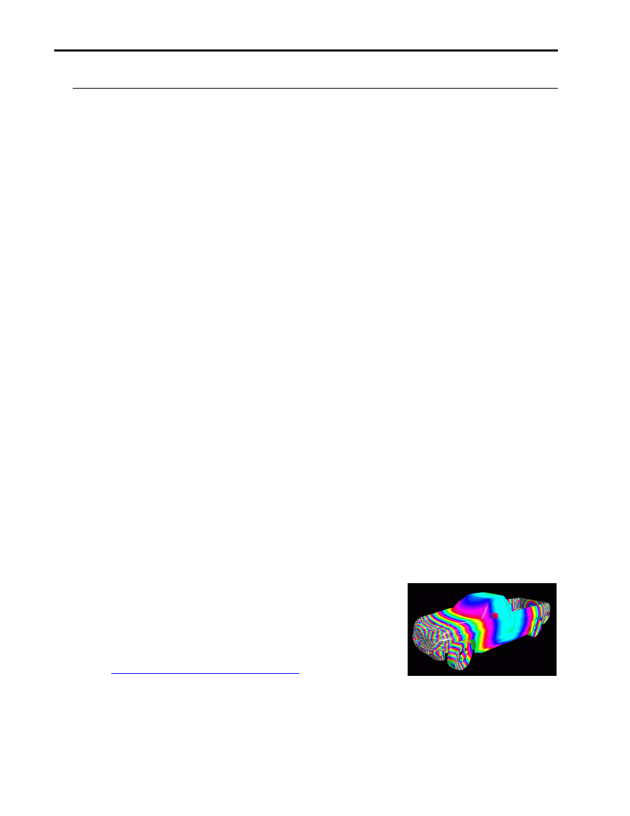
ProCDRS
The ProCDRS-01 viewset is a complete update of the CDRS-
03 viewset. It is intended to model the graphics performance of
Parametric Technology Corporation's Pro/DESIGNER
industrial design software.
For more information on Pro/DESIGNER, see
http://www.ptc.com/products/indu/id.htm
The viewset consists of ten tests, each of which represents a
different mode of operation within Pro/DESIGNER. Two of the tests use a wireframe model, and
the other tests use a shaded model. Each test returns a result in frames per second, and a
Graphics Performance: Measures, Metrics and Meaning
15
0052-0499-A
composite score is calculated as a weighted geometric mean of the individual test results. The
tests are weighted to represent the typical proportion of time a user would spend in each mode.
The model data was converted from OpenGL command traces taken directly from the running
Pro/DESIGNER software, and therefore preserves most of the attributes of the original model.
This viewset uses new features that require Viewperf v6.x.
The shaded model is a mixture of triangle stips and independent triangles, with approximately
281000 vertices in 4700 OpenGL primitives, giving 131000 triangles total. The average triangle
screen area is 4-5 pixels.
The wire frame model consists of only line strips, with around 202000 vertices in 19000 strips,
giving 184000 lines total.
All tests run in display list mode. The wireframe tests use anti-aliased lines, since these are the
default in Pro/DESIGNER. The shaded tests use one infinite light and two-sided lighting. The
texture is a 512 by 512 pixel 24-bit color image. See the script files for more information.
Test
Weight Description
1
25
Wireframe test
2
25
Wireframe test, walkthrough
3
10
Shaded test
4
10
Shaded test, walkthrough
5
5
Shaded with texture
6
5
Shaded with texture, walkthrough
7
3
Shaded with texture, eye linear texgen (dynamic reflections)
8
3
Shaded with texture, eye linear texgen, walkthrough
9
7
Shaded with color per vertex
10
7
Shaded with color per vertex, walkthrough
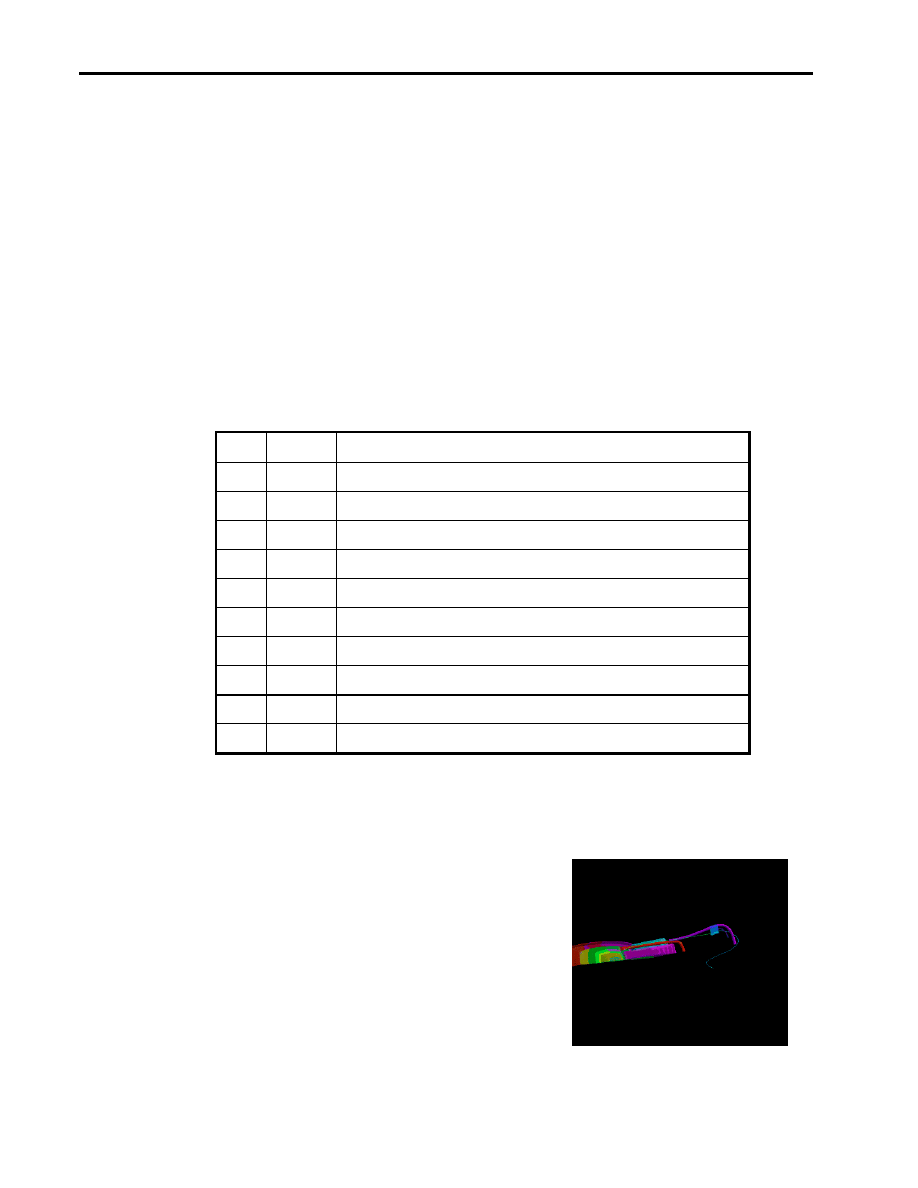
CDRS
CDRS has been retired, and results are no longer reported.
It is included here because of its widespread use in the past.
CDRS is Parametric Technology's modeling and rendering
software for computer-aided industrial design (CAID). It is
used to create concept models of automobile exteriors and
interiors, other vehicles, consumer electronics, appliances
and other products that have challenging free-form shapes.
The users of CDRS are typically creative designers with job
titles such as automotive designer, products designer or
industrial designer.
Graphics Performance: Measures, Metrics and Meaning
16
0052-0499-A
There are seven tests specified that represent different types of operations performed within
CDRS. Five of the tests use a triangle strip data set from a lawnmower model created using
CDRS. The other two tests show the representation of the lawnmower.
The tests are weighted and show the following CDRS functionality:
*
Test
*
Weight
*
CDRS functionality represented
*
1
50%
Vectors used in designing the model. Represents most of
the design work done in CDRS. Antialiasing turned on to
allow the designer to see a cleaner version of the model.
*
2
20%
Surfaces shown as polygons, but all with a single surface
color.
*
3
15%
Surfaces grouped with different colors per group.
*
4
8%
Textures added to groups of polygons.
*
5
5%
Texture used to evaluate surface quality.
*
6
2%
Color added per vertex to show the curvature of the surface.
*
7
0%
Same as test #1, but without the antialiasing.
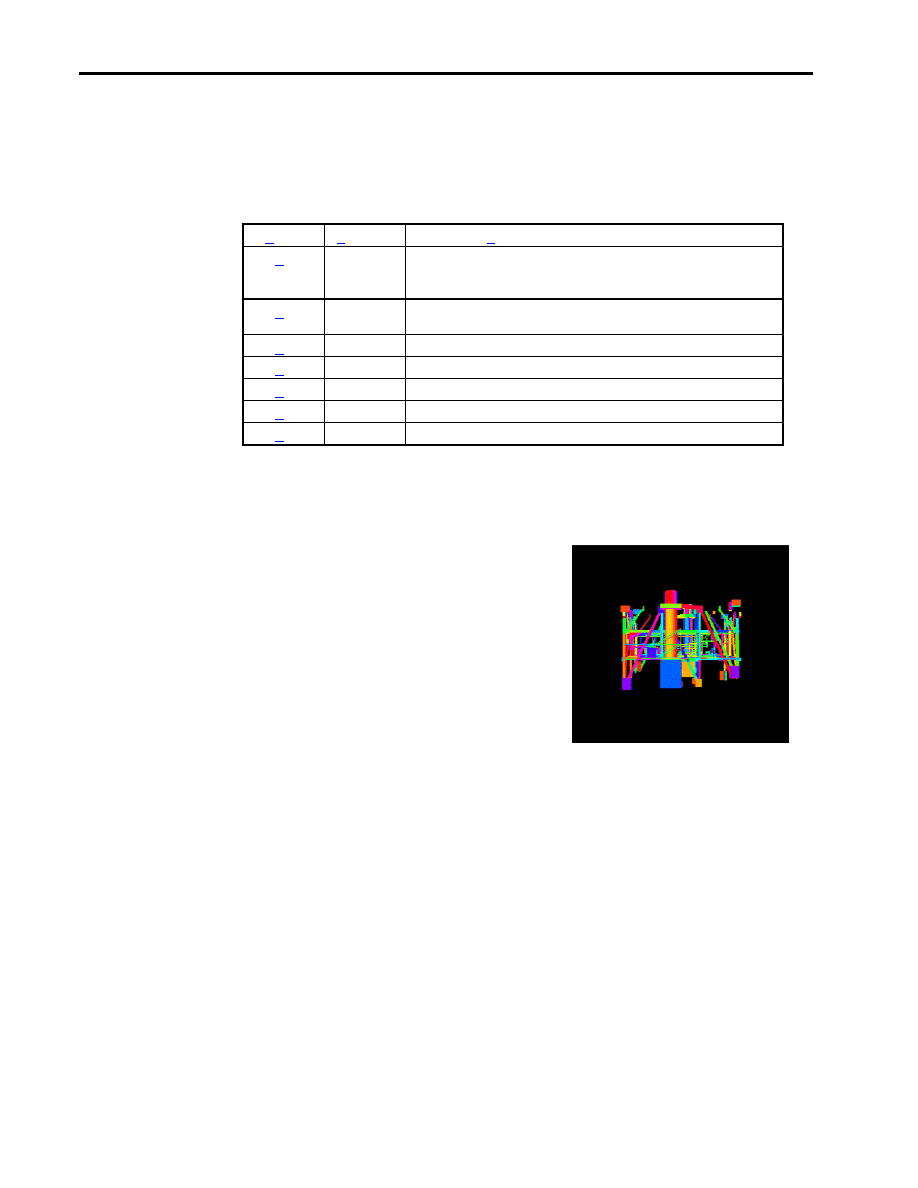
DRV
DesignReview is a 3D computer model review package
specifically tailored for plant design models consisting of
piping, equipment and structural elements such as I-beams,
HVAC ducting, and electrical raceways. It allows flexible
viewing and manipulation of the model for helping the
design team visually track progress, identify interferences,
locate components, and facilitate project approvals by
presenting clear presentations that technical and non-
technical audiences can understand.
On the construction site, DesignReview can display
construction status and sequencing through vivid graphics that complement blueprints. After
construction is complete, DesignReview continues as a valuable tool for planning retrofits and
maintenance. DesignReview is a multi-threaded application that is available for both UNIX and
Windows NT.
The model in this viewset is a subset of the 3D plant model made for the GYDA offshore oil
production platform located in the North Sea on the southwest coast of Norway. A special thanks
goes to British Petroleum, which has given the OPC subcommittee permission to use the
geometric data as sample data for this viewset. Use of this data is restricted to this viewset.
DesignReview works from a memory-resident representation of the model that is composed of
high-order objects such as pipes, elbows valves, and I-beams. During a plant walkthrough, each
view is rendered by transforming these high-order objects to triangle strips or line strips.
Tolerancing of each object is done dynamically and only triangles that are front facing are
generated. This is apparent in the viewset model as it is rotated.
Most DesignReview models are greater than 50 megabytes and are stored as high-order objects.
For this reason and for the benefit of dynamic tolerancing and face culling, display lists are not
used.
Graphics Performance: Measures, Metrics and Meaning
17
0052-0499-A
There are 6 tests specified by the viewset that represent the most common operations performed
by DesignReview. These tests are as follows:
*
Test
*
Weight
*
DRV functionality represented
*
1
45%
Walkthrough rendering of curved surfaces. Each curved
object (i.e., pipe, elbow) is rendered as a triangle mesh,
depth-buffered, smooth-shaded, with one light and a
different color per primitive.
*
2
30%
Walkthrough rendering of flat surfaces. This is treated as a
different test than #1 because normals are sent per facet and
a flat shade model is used.
*
3
8%
For more realism, objects in the model can be textured. This
test textures the curved model with linear blending and
mipmaps.
*
4
5%
Texturing applied to the flat model.
*
5
4%
As an additional way to help visual identification and
location of objects, the model may have "screen door"
transparency applied. This requires the addition of polygon
stippling to test #2 above.
*
6
4%
To easily spot rendered objects within a complex model, the
objects to be identified are rendered as solid and the rest of
the view is rendered as a wireframe (line strips). The line
strips are depth-buffered, flat-shaded and unlit. Colors are
sent per primitive.
*
7
4%
Two other views are present on the screen to help the user
select a model orientation. These views display the position
and orientation of the viewer. A wireframe, orthographic
projection of the model is used. Depth buffering is not used,
so multithreading cannot be used; this preserves draw order.
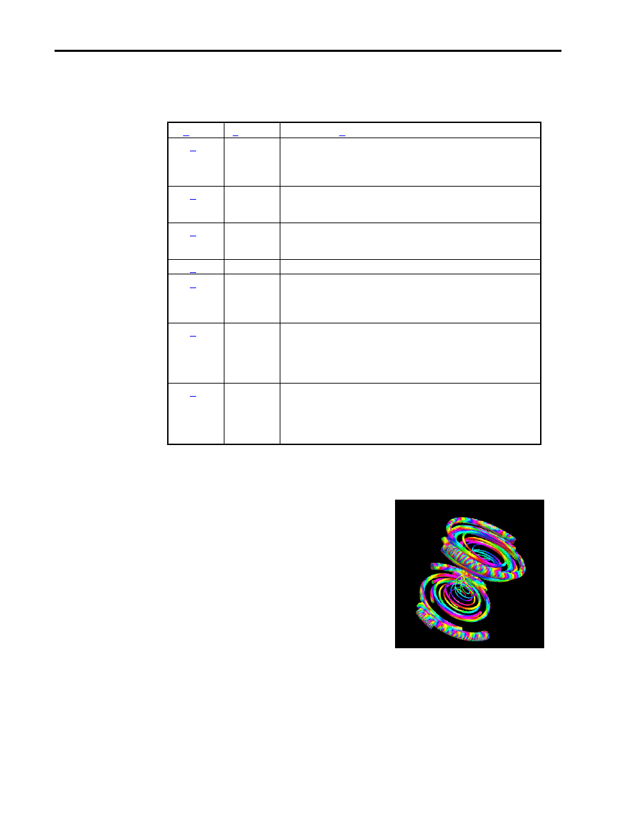
DX
The IBM Visualization Data Explorer (DX) is a general-
purpose software package for scientific data visualization
and analysis. It employs a data-flow driven client-server
execution model and is currently available on Unix
workstations from Silicon Graphics, IBM, Sun, Hewlett-
Packard and Digital Equipment. The OpenGL port of Data
Explorer was completed with the recent release of DX 2.1.
The tests visualize a set of particle traces through a vector
flow field. The width of each tube represents the magnitude
of the velocity vector at that location. Data such as this
might result from simulations of fluid flow through a
constriction. The object represented contains about 1,000 triangle meshes containing
approximately 100 verticies each. This is a medium-sized data set for DX.
Test Weighting
All tests assume z-buffering with one light in addition to specification of a color at every vertex.
Triangle meshes are the primary primitives for this viewset. While Data Explorer allows for many
other modes of interaction, these assumptions cover the majority of user interaction.
Graphics Performance: Measures, Metrics and Meaning
18
0052-0499-A
The first version of this viewset included indirect rendering to handle the client/server model of
X-Windows-based systems. In this version, tests with indirect rendering have been removed to
allow the viewset to be fully ported to Windows NT and OS/2 environments.
*
Test
*
Weight
*
DX functionality represented
*
1
40%
TMESH's immediate mode.
*
2
20%
LINE's immediate mode.
*
3
10%
TMESH's display listed.
*
4
8%
POINT's immediate mode.
*
5
5%
LINE's display listed.
*
6
5%
TMESH's list with facet normals.
*
7
5%
TMESH's with polygon stippling.
*
8
2.5%
TMESH's with two sided lighting.
*
9
2.5%
TMESH's clipped.
*
10
2%
POINT's direct rendering display listed.
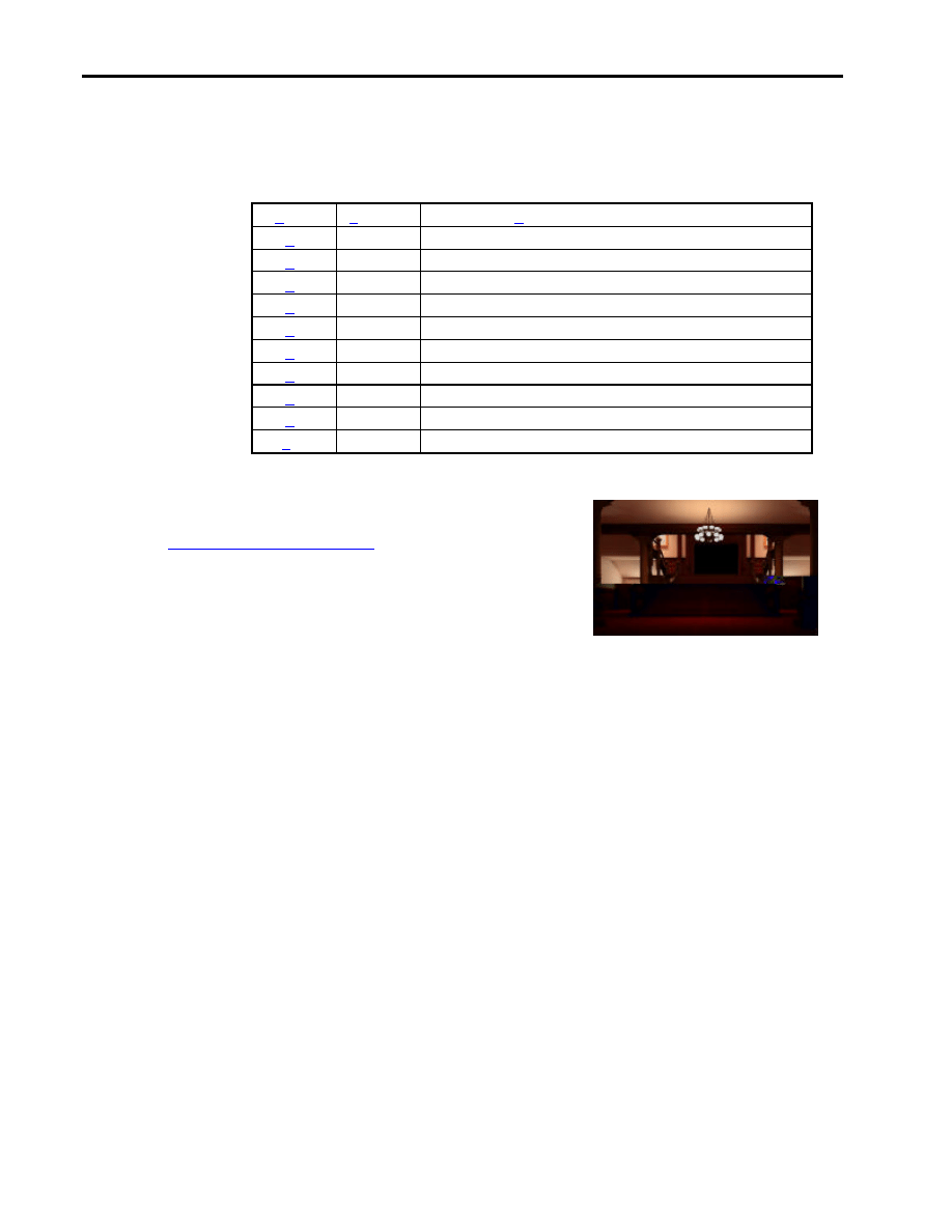
LIGHT
The Lightscape Visualization System from
Lightscape Technologies, Inc.
represents a new generation
of computer graphics technology that combines proprietary
radiosity algorithms with a physically based lighting
interface.
Lighting
The most significant feature of Lightscape is its ability to accurately simulate global illumination
effects. The system contains two integrated visualization components. The primary component
utilizes progressive radiosity techniques and generates view-independent simulations of the
diffuse light propagation within an environment. Subtle but significant effects are captured,
including indirect illumination, soft shadows, and color bleeding between surfaces. A post
process using ray tracing techniques adds specular highlights, reflections, and transparency
effects to specific views of the radiosity solution.
Interactivity
Most rendering programs calculate the shading of surfaces at the time the image is generated.
Lightscape's radiosity component precalculates the diffuse energy distribution in an environment
and stores the lighting distribution as part of the 3D model. The resulting lighting "mesh" can
then be rapidly displayed. Using OpenGL display routines, Lightscape takes full advantage of the
advanced 3D graphics capabilities of SGI workstations or PC-based OpenGL-compliant graphic
acceleration boards. Lightscape allows you to interactively move through fully simulated
environments.
Progressive Refinement
Lightscape utilizes a progressive refinement radiosity algorithm that produces useful visual
results almost immediately upon processing. The quality of the visualization improves as the
process continues. In this way, the user has total control over the quality (vs. time) desired to
Graphics Performance: Measures, Metrics and Meaning
19
0052-0499-A
perform a given task. At any point in the solution process, users can alter the characteristic of a
light source or surface material and the system will rapidly compensate and display the new
results without the need for restarting the solution. This flexibility and performance allow users to
rapidly test various lighting and material combinations to obtain precisely the visual effect
desired.
There are four tests specified by the viewset that represent the most common operations
performed by the Lightscape Visualization System:
*
Test
*
Weight
*
DRV functionality represented
*
1
25%
Walkthrough wireframe rendering of "Cornell Box" model
using line loops with colors supplied per vertex.
*
2
25%
Full-screen walkthrough solid rendering of "Cornell Box"
model using smooth-shaded z-buffered quads with colors
supplied per vertex.
*
3
25%
Walkthrough wireframe rendering of 750K-quad Parliament
Building model using line loops with colors supplied per
vertex.
*
4
25%
Full-screen walkthrough solid rendering of 750K-quad
Parliament Building model using smooth-shaded z-buffered
quads with colors supplied per vertex.
AWADVS
Advanced Visualizer from
Alias/Wavefront
is an
integrated workstation-based 3D animation system that
offers a comprehensive set of tools for 3D modeling,
animation, rendering, image composition, and video output.
The Advanced Visualizer provides:
•
Geometric, analysis, and motion data
importation from a wide range of CAD,
dynamics and structural systems.
•
Automatic object simplification and switching
tools for working with ultra-large production data sets.
•
Motion for an unlimited number of objects, cameras, and lights with Wavefront
SmartCurve editing techique.
•
Interactive test rendering and high-quality, free-form surface rendering
•
Software rotoscoping for matching computer animation with live action background
footage.
•
Realistic imaging effects, including soft shadows, reflection, refraction, textures, and
displacememt maps, using Wavefront's fast hybrid scanline/raytracing renderer.
•
Interactive image layering and output to video with Wavefront's new Recording
Composer.
Graphics Performance: Measures, Metrics and Meaning
20
0052-0499-A
•
Powerful scripting and customization tools, open file formats, and user-defined
interfaces.
For more information on Advanced Visualizer, please visit the Alias/Wavefront
Advanced Visualizer
web page.
There are 10 tests specified by the viewset that represent the most common operations performed
by Advanced Visualizer:
*
Test
*
Weight
*
Advanced Visualizer functionality represented
*
1
41.8%
Material shading of polygonal animation model with
highest interactive image fidelity and perspective
projection.
*
2
28.5%
Wireframe rendering of polygonal animation model with
perspective projection.
*
3
10.45%
Material shading of polygonal animation model with lowest
interactive image fidelity and perspective projection.
*
4
9.5%
Smooth shading of polygonal animation model with
perspective projection.
*
5
4.75%
Flat shading of polygonal animation model with perspective
projection.
*
6
2.2%
Material shading of polygonal animation model with
highest interactive image fidelity and orthogonal projection.
*
7
1.5%
Wireframe rendering of polygonal animation model with
orthogonal projection.
*
8
.55%
Material shading of polygonal animation model with lowest
interactive image fidelity and orthogonal projection.
*
9
.5%
Smooth shading of polygonal animation model with
orthogonal projection.
*
10
.25%
Flat shading of polygonal animation model with orthogonal
projection.

Graphics Performance: Measures, Metrics and Meaning
21
0052-0499-A
Appendix 2: Indy3D Benchmark
A new benchmark that is growing in popularity is the Indy3D benchmark from Sense8 and
Mitsubishi. Sense8 has developed a high level graphical toolkit called World Toolkit that is used
to develop graphically intensive applications. To measure the performance of different systems
in running applications built on World Toolkit, Sense8 worked with several of their application
partners to develop benchmarks that represent different types of applications. The resulting suite
of benchmarks is called Indy3D.
Indy3D addresses application performance for mechanical CAD (with small and large assembly
models), visual simulation and animation. Indy3D also provides an image quality test and a set of
primitive tests for measuring low level performance.
Like ViewPerf, this benchmark also uses graphical data derived from real applications, but builds
more complete scenes. Were ViewPerf uses a series of independent tests, and then combines the
results to produce a composite performance number, Indy3D combines all the tests for an
application type into a single run, and produces a single number for this run.
As a result of being newer than ViewPerf, Indy3D addresses recent trends in graphics. These
include a strong focus on texture mapped scenes and large assembly models.
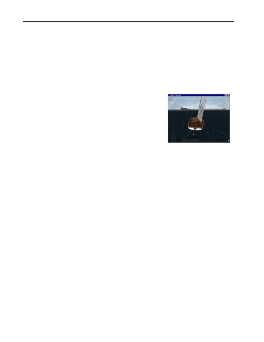
Indy3D also has the advantage of being a more visually interesting test. Each test case is
interesting to watch – the MCAD test moves and manipulates an automobile engine, the visual
simulation test has a sailboat racing about San Francisco bay, and the animation test has a person
walking through a graffiti strewn city street. While not adding to the technical significance of the
tests, this approach makes it easier to relate to graphics performance – the test is intuitive to
understand, and easy to visually gauge the performance of a system.
One of the strengths of Indy3D is its visual quality test. This test provides insight into the quality
of the graphics hardware and drivers. It displays a scene that exercises many aspects of OpenGL
graphics – lighting, shading, texture interpolation, blending, precision, and performance. While it
is not a definitive measure of graphical quality, it provides a useful tool.
One last difference between Indy3D and ViewPerf is in ownership and control of the benchmark.
ViewPerf is maintained by an industry consortium, is developed and approved by representatives
from many companies, is available in source form, and runs on a wide range of platforms.
Indy3D is the product of a single company, is delivered as an executable program without source
code, and is supported on a limited range of platforms.
From information included in Indy3D:
Overview
The Indy3D benchmark evaluation tool is focused on three segments of the 3D graphics market,
MCAD, Animation, and Simulation. We built this benchmark because we live in this market
space and none of the existing benchmark tools provide the information we like to know. We
hope typical users in each of the three areas can easily use these benchmark results to gauge their
needs and find a board or system that fulfills them. The Indy3D graphics evaluation tool was
constructed to aid end-users in evaluating OpenGL 3D performance issues using application-
focused metrics (MCAD, animation and simulation markets), image quality stress tests and 3D
primitive metrics. Indy3D was constructed out of the desire to have a single tool that provided

Graphics Performance: Measures, Metrics and Meaning
22
0052-0499-A
simple comparative measurements while allowing the user to explore various rendering options
and perform their own ad hoc tests. Indy3D produces four official results; two for the MCAD
tests (MCAD40, MCAD150) and one each for the animation and simulation tests. Sense8
maintains a web site that allows users to compare their results with other platforms that have been
verified by Sense8. By providing this verified information, we hope users will easily understand
the value other 3D accelerator solutions provide for typical application problems.
Unique features of Indy3D:
Designed for users with limited real-time 3D rendering background
•
Single test result for each application test (MCAD, simulation, animation)
generated within minutes
•
Image Quality test reveals image details that are often overlooked or never
understood
•
Official measurements made on a single reference system to remove system
dependencies
•
Combination of multiple application and primitive measurements in a single
benchmark
•
Automatic generation of test images from test run to compare with reference
images
•
Results generated as HTML, includes reference AVIs/images
Methodology in general
All the user methodology tests represent an informed opinion about how the chosen markets use
real-time 3D techniques for typical uses. Sense8 relied not only on its own experience in these
markets but also derived this from long discussions with experts and 3D analysts who represent
these markets. While Indy3D attempts to measure a broad "typical" use in order to keep the
measurements fast, simple and understandable, you should also realize that no one tool will
represent all uses.
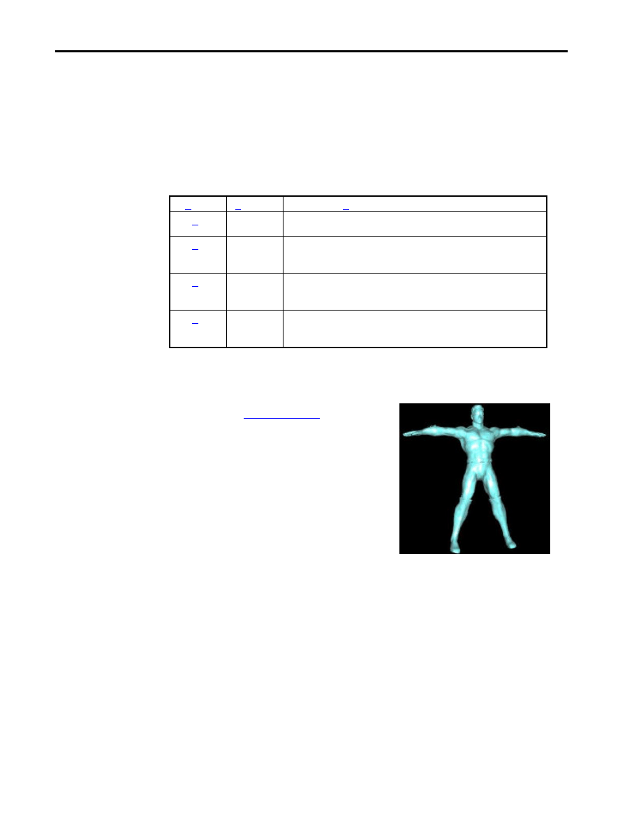
MCAD benchmark
The MCAD benchmark test consists of two different tests
(MCAD40 and MCAD150) designed to simulate the rendering
of typical models of medium to high complexity (40,000 or
150,000 polygons). The MCAD150 test has enough polygons
that it tends to give results highly dependent on the CPU or
geometry transformation hardware and little else. The entire
engine database is converted to an OpenGL display list prior to
testing. Note: PTC and Microstation don't use display lists, but
CDRS and SDRC do. This means there are some CAD
applications that do not take advantage of display lists and therefore Indy3D may not be
applicable in these cases. There is no way to test the engine database in immediate mode. You
should also know that display lists vs immediate mode makes the greatest difference when the
hardware has a display-list cache of significant size (like SGI IR or HP Fx series).
Graphics Performance: Measures, Metrics and Meaning
23
0052-0499-A
The MCAD visual database is an engine model supplied by Engineering Animation Incorporated
(EAI). The engine was created with SDRC's IDEAS Master Series and was converted into a
VRML 1.0 file using EAI’s VisMockup application.
MCAD40 Database notes:
•
Contains 42,267 polygons, all polygons are single-sided
•
Contains an assembly of lower level components (149 geometries)
•
Average pixel size of rendered polygons is 30 pixels
•
Average depth complexity of the entire scene is 0.52 pixel overwrites per frame
•
Average polygons drawn per frame (non-culled polygons) is 42,120
•
Database is converted to an OpenGL display list comprised of over 12,035
triangle strip sets (average size of 3 triangles)
•
MCAD150 Database notes:
•
Contains 150,248 polygons, all polygons are single-sided
•
Contains an assembly of lower level components (149 geometries)
•
Average pixel size of rendered polygons is 9 pixels
•
Average depth complexity of the entire scene is 0.52 pixel overwrites per frame
•
Average polygons drawn per frame (non-culled polygons) is 149,786
•
Database is converted to an OpenGL display list comprised of over 48,257
triangle strip sets (average size of 3 triangles)
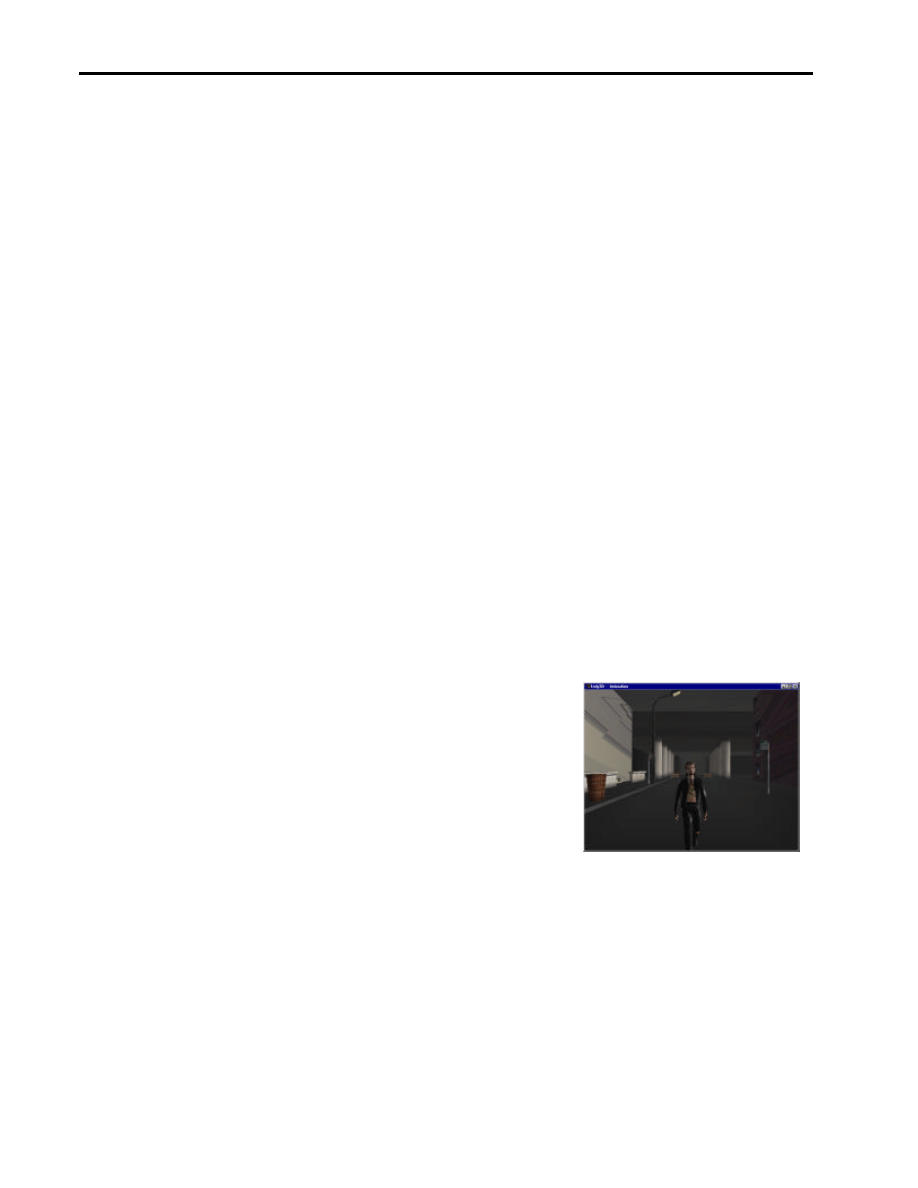
Animation
The Animation model is a human figure supplied by the
Westwood Studios. We feel this type of character-based
modeling is typical of the game and video animation
markets. The cityscape around the figure was created by
Sense8 to put the figure in a typical setting. The file supplied
by Westwood Studios was in 3D Max format and was then
processed by Sense8 to eliminate redundant polygons and
stored in a compact Sense8 format. The animation database
is not converted to an OpenGL display list, it remains in
immediate mode which is the norm for all Animation tools.
Database notes:
•
Contains 133,004 polygons for the entire scene (all 133K polygons are never
rendered at once, a switch node selects about 24,000 polygons for consideration
during any single frame)
•
The human figure contains about 22,000 single-sided polygons as a single mesh
•
The cityscape contains 2,381 single-sided polygons divided into 41 geometries
•
There are no level-of-detail nodes
Graphics Performance: Measures, Metrics and Meaning
24
0052-0499-A
•
There is a switch node, which cycles through the six geometries of the character
(about 22,000 polygons each) to create movement.
•
Texture database size is 2.72Mb comprised of a mix of resolution sizes
•
Average pixel size of rendered polygons is 140 pixels
•
Average depth complexity of the scene is 1.35 pixel overwrites per frame
•
Average polygons drawn per frame (non-culled polygons) is 22,865 polygons
Simulation
We have selected a realistic sailing simulation built by
Sense8. The sailboat is driven forwards by wind forces acting
on the boat and by resistance of the boat to the water. The
physics involved in this simulation are fairly simple and we
have verified that on the reference system, the impact of
running the physics simulation is not noticeable with any of
the graphics boards we tested at the official settings.
However, it is possible that for smaller windows or boards
with extremely large texture fill capabilities (anything that
can deliver 25-35 fps for the simulation), the impact of the
physics model will be felt if the CPU can't keep up with the rendering and becomes the
bottleneck. The justification for this is that in the simulation market, there is almost always some
CPU utilization for running code other than 3D transformations/lightings.
In addition to the physics simulation, we are creating "waves" by moving the vertices of a mesh
of polygons near the boat. We have verified that this makes a negligible contribution to
performance under most expected environments.
Database notes:
•
Contains 7,710 polygons in a mix of single and both-sided polygons
•
Contains 61 geometries in a mix of single and both-sided polygons
•
There are no level-of-detail nodes
•
Texture database size is 3.64Mb comprised of a mix of resolution sizes
•
Average pixel size of rendered polygons is 574 pixels
•
Average depth complexity of the scene is 2.15 pixel overwrites per frame
•
Average polygons drawn per frame (non-culled polygons) is 7257 polygons per
frame
•
The non-wave portion of the database is converted to an OpenGL display list
comprised of over 75 triangle strip sets
Image Quality test
This test is designed to identify specific rendering issues with various OpenGL implementations.
There are ten special regions in the image (see below). Each region of the image is designed to
reveal particular issues related to the processing of texels (the pixels that comprise a texture map)

Graphics Performance: Measures, Metrics and Meaning
25
0052-0499-A
or polygons. There is no specific "performance" measurement for this test. It is very difficult to
algorithmically calculate the quality of an image, so we have left it to a subjective analysis. The
intent is for you to look at the image generated by your hardware and compare it to a reference
image that we believe best represents what OpenGL should have created. In addition, every time
you press the "Run Test" button, your viewpoint will "bounce" into the picture and then an image
will be captured and stored on your hard drive for later comparison.
Primitive Tests
The purpose of the three primitive tests is to help you understand lower-level issues related to
real-time 3D rendering. In general, most real-time 3D systems are either limited by the rate at
which they can push pixels to the screen (fill rate) or they are limited by the rate at which the
system (board/CPU) can transform/light the polygons (triangle rate). These two primary issues
interrelate making the picture fairly complex. These tests help you gain insight into these
fundamental issues and may explain why your system is achieving a particular score for the user
tests.
Hardware manufacturers like to publish primitive measurements gathered with various tools that
are optimized for achieving the highest number. In general, this kind of benchmarking rarely
represents typical use. Our primitive tests are geared more towards "application" polygons so
don't expect the manufacturers numbers to necessarily agree with our results.
Fill Rate
The fill rate test measures the speed or bandwidth of the graphics hardware to draw pixels. This is
measured in millions of pixels per second. To achieve high frame-rates when rendering high-
resolution images requires significant bandwidth. Rendering a single polygon that fills a 1024 x
768 window at 10 Hz requires 7.8 Mpixels per second bandwidth. Typical databases require two
to four times this amount. This test measures the pixel fill rate by introducing a stack of polygons
(with vertex normals and vertex colors) drawn back to front (the most difficult condition) that are
viewed orthographically. This test automatically introduces additional polygons until the frame
rate drops below 10 hz. Once the frame-rate is below 10, the test measures 30 frames and
calculates the current fill rate. Along with the various rendering options, you can measure a wide
range of fill values.
Fixed Rate
The fixed rate test is targeted for the simulation community and measures the number of polygons
rendered at 20 Hz. This is an important measurement as it drives the acceptable size and design of
the visual database used for a simulation. This is measured by introducing sets of triangles (vertex
normals, but no vertex colors) until the desired frame rate of 20 +/- 0.5 Hz is achieved. Once this
frame rate is achieved, it must be sustained for 5 seconds. The view is drawn orthographically.
Additional sets of polygons are added by stacking them on top of each other (rendering
performed in back to front order), but offset by 10 units (to avoid coplanar polygons).
NOTE: Indy3D Version2.0 rendered polygons front-to-back instead of back-to-front. This was
changed in Indy3D Version2.2. Some hardware is optimized to take advantage of the rendering
order and this may cause results to change with Indy V2.2.

Graphics Performance: Measures, Metrics and Meaning
26
0052-0499-A
Polygon Rate
The polygon rate test measures triangles per second and stresses the underlying transform,
lighting, and setup calculations of the system and graphics board. For databases composed of tens
of thousands of polygons, this typically becomes the limiting factor in achieving better
performance. In addition to graphics board issues, the underlying CPU and system performance
significantly influences this measurement. The measurement occurs by introducing sets of
triangles (vertex normals, but no vertex colors) until the frame rate drops below 10 Hz. Once this
frame rate is achieved, the measurement is performed over 30 frames. The view is be drawn
orthographically. Additional sets of polygons are added by stacking them on top of each other
(rendering performed in back to front order), but offset by 10 units (to avoid coplanar polygons).
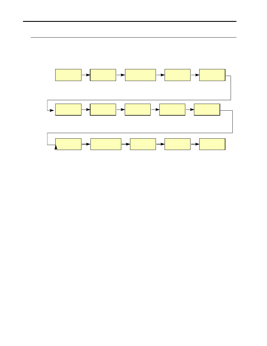
Graphics Performance: Measures, Metrics and Meaning
27
0052-0499-A
Appendix 3: The Graphics Pipeline
Display
Traversal
Modeling
Transform
Trivial
Accept/Reject
Lighting
Viewing
Transform
Clipping
Divide by
W
Viewport
Mapping
Span
Generation
Triangle
Setup
Texture
Mapping
Scan
Convert
Z
Buffer
Display
Texture
Lookup
This diagram shows a typical graphics pipeline. For more details, see a graphics reference such
as “Fundamentals of Computer Graphics” by Foley and van Damm.
Display traversal is an application level function, and varies by application. The result of this
phase is low level geometry primitives ready for input to the graphics pipeline.
The transformations are 4x4 matrix operations. They involve 13 floating point multiplications,
13 floating point additions and the movement of all required data. Transforms may be applied to
an entire part, or to individual vertices in a part. This transform, the viewing transform, and the
lighting calculations, are the most computationally intensive part of the graphics pipeline.
Trivial accept/reject is used to discard objects that can not possibly appear in a view. This stage
can dramatically improve graphics performance.
Texture mapping establishes the relationship between a 3D XYZ coordinate on the surface and a
2D UV coordinate in a texture map. Several algorithms are commonly used; all are complex and
require extensive floating point computation.
Lighting calculations require calculating a surface normal and a direction vector between the
light and the point on the surface and performing trigonometric calculations between the surface
normal and the light direction vector. This is performed for each light. Advanced lighting may
involve many additional calculations.
The viewing transform is the same as the model transform.
Clipping involves checking to see if a graphics object is entirely within the view. An object may
be discarded, may be entirely drawn, or may be trimmed to the edge of the viewport.
Perspective correction is applied for perspective view. This involves a floating point division,
based on the Z distance from the viewing plane to the object.
Viewport mapping is simply determining which viewport (or window) to display in and which
screen coordinates to use.
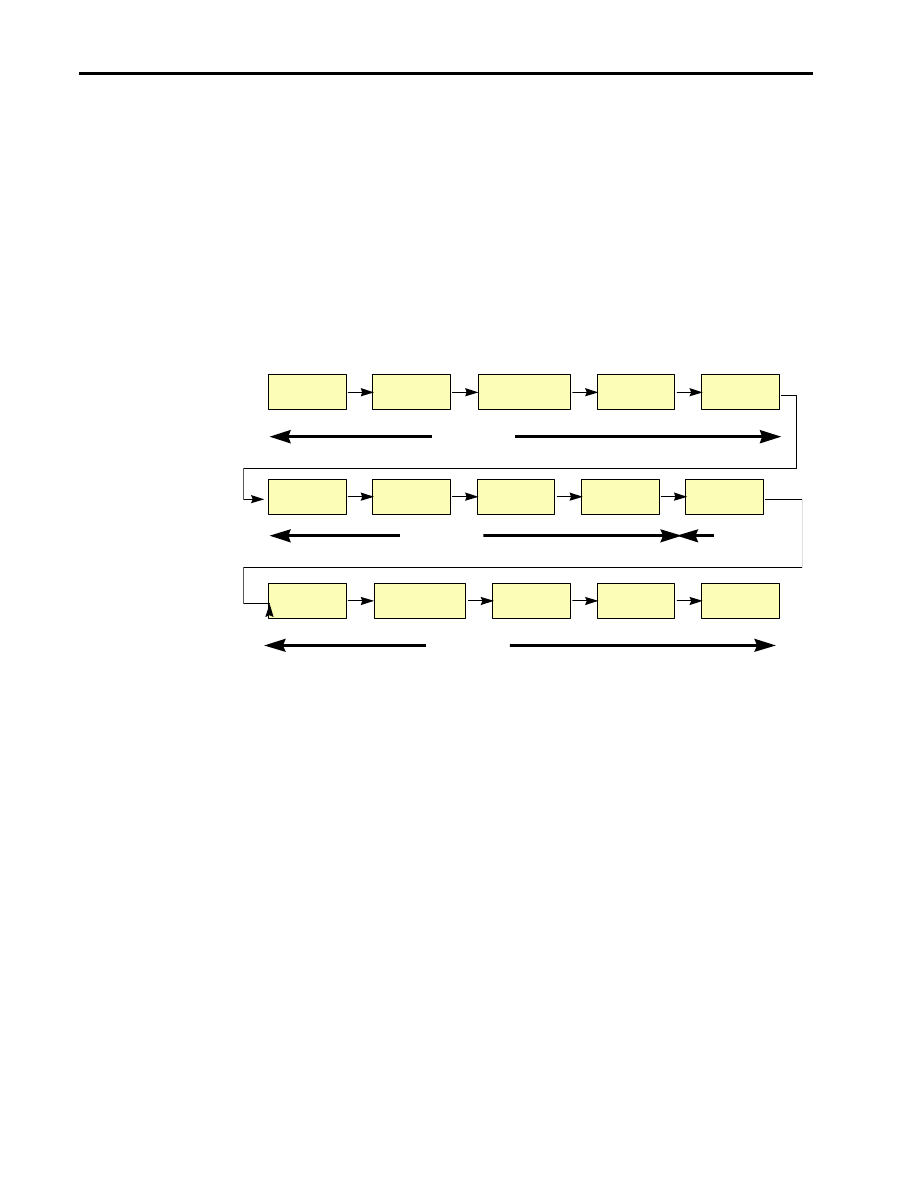
Graphics Performance: Measures, Metrics and Meaning
28
0052-0499-A
Triangle setup is the first step in display interpolation. The three vertices of the triangle (with
associated information) are defined. The edges of the triangle are interpolated (slope
calculations) to produce values (XYZ, RGBA, UV) for each end of each span line.
If texturing is being done, lookup of the UV coordinate in the desired texture map is performed
for each pixel. Bilinear and trilinear interpolation will require multiple lookups and averaging.
Span conversion involves taking values at each end of the span line and interpolating to calculate
the values at each individual pixel.
Z-buffering involves comparing the Z value of the new pixel with the previous pixel, and
discarding the one that is furtherest from the eyepoint.
Finally, the RGB value of each individual pixel is ready for display.
Display
Traversal
Modeling
Transform
Trivial
Accept/Reject
Lighting
Viewing
Transform
Clipping
Divide by
W
Viewport
Mapping
Span
Generation
Triangle
Setup
Texture
Mapping
Scan
Convert
Z
Buffer
Display
Texture
Lookup
Software
Software
Hardware
Hardware
On the PowerStorm 300, high level calculations are done in software on the host processor, and
low level operations are done in the graphics hardware.

Graphics Performance: Measures, Metrics and Meaning
29
0052-0499-A
Appendix 4: Additional Resources
•
Computer Graphics: Principles and Practice by Foley, van Dam, Feiner and Hughes. This is the
standard textbook on computer graphics, providing quality explanations of all aspects of 2D and 3D
graphics algorithms with many implementation notes. Not recommended for casual reading, but an
excellent reference.
•
The SpecBench Web site at
http://www.specbench.org
contains the full set of ViewPerf performance
data and is regularly updated. This site also contains the SpecINT and SpecFP benchmarks for CPU
performance.
•
http://www.compaq.com
/workstation contains a variety of information on Compaq workstation and
graphics offerings.
•
http://www.siggraph.org
is the Web site for ACM SIGGRAPH, the Special Interest Group for
Graphics. SIGGRAPH has long been one of the leading organizations for sharing information on
graphics technology, algorithms, and developments.
•
http://www.opengl.org
contains a wide range of information on OpenGL and links to much more
information. This is an excellent starting point for delving into OpenGL.
•
http://www.sense8.com/indy3d/index.html
contains a downloadable kit for the Indy3D benchmark,
as well as performance data for a number of systems and graphics boards.
Wyszukiwarka
Podobne podstrony:
KONWENCJA BERNEŃSKA, MiBM Politechnika Poznanska, VII semestr TPM, Ochrona Własności Intelektualnej,
Pojęcia, MiBM Politechnika Poznanska, VII semestr TPM, Ochrona Własności Intelektualnej, wojtysiak,
TPM
IMG 0052
odlewnicze stopy aluminium i ich obrobka cieplna-struktury, Studia, SEMESTR 3, TPM
Rodzaje utworów chronionych prawem autorskim, MiBM Politechnika Poznanska, VII semestr TPM, Ochrona
tpm notatka
notatka-pvd, Studia, SEMESTR 3, TPM
Utwory pracownicze, MiBM Politechnika Poznanska, VII semestr TPM, Ochrona Własności Intelektualnej,
TPM
pompy tp tpm k
najważniejsze podmioty, MiBM Politechnika Poznanska, VII semestr TPM, Ochrona Własności Intelektual
OWI full test, MiBM Politechnika Poznanska, VII semestr TPM, Ochrona Własności Intelektualnej, wojty
Rotomoulding, Studia, SEMESTR 3, TPM, prezentacja polimery, formowanie
1.abcd, MiBM Politechnika Poznanska, VII semestr TPM, Ochrona Własności Intelektualnej, wojtysiak, O
Maszyny stosowane w technologii odlewania rotacyjnego, Studia, SEMESTR 3, TPM, prezentacja polimery,
ZAS PRZYWIL KOMUNIKACYJNEGO, MiBM Politechnika Poznanska, VII semestr TPM, Ochrona Własności Intelek
więcej podobnych podstron