Parlour And Seppi Liquidity Based Competition For Order Flow

Liquidity-Based Competition
for Order Flow

Christine A. Parlour
Carnegie Mellon University

Duane J. Seppi
Carnegie Mellon University

We present a microstructure model of competition for order flow between exchanges
based on liquidity provision. We find that neither a pure limit order market (PLM) nor
a hybrid specialist/limit order market (HM) structure is competition-proof. A PLM can
always be supported in equilibrium as the dominant market (i.e., where the hybrid limit
book is empty), but an HM can also be supported, for some market parameterizations,
as the dominant market. We also show the possible coexistence of competing markets.
Order preferencing—that is, decisions about where orders are routed when investors are
indifferent—is a key determinant of market viability. Welfare comparisons show that
competition between exchanges can increase as well as reduce the cost of liquidity.

Active competition between exchanges for order flow in cross-listed securi-
ties is intense in the current financial marketplace. Examples include rival-
ries between the New York Stock Exchange (NYSE), crossing networks,
and ECNs and between the London Stock Exchange, the Paris Bourse, and
other continental markets for equity trading and between Eurex and London
International Financial Futures and Options Exchange (LIFFE) for futures
volume. While exchanges compete along many dimensions (e.g., “payment
for order flow,” transparency, execution speed), liquidity and “price improve-
ment” will, in our view, be the key variables driving competition in the future.
Over time, high-cost markets should be driven out of business as investors
switch to cheaper trading venues. Moreover, “market structure” is increas-
ingly singled out by regulators, exchanges, and other market participants as
a major determinant of liquidity.

We thank the editor, Larry Glosten, for many helpful insights and suggestions. We also benefited from
comments from Shmuel Baruch, Utpal Bhattacharya, Bruno Biais, Wolfgang Bühler, David Goldreich, Rick
Green, Burton Hollifield, Ronen Israel, Craig MacKinlay, Uday Rajan, Robert Schwartz, George Sofianos,
Tom Tallarini, Jr., Josef Zechner, as well as from seminar participants at the Catholic University of Louvain,
London Business School, Mannheim University, Stockholm School of Economics, Tilburg University, Uni-
versity of Utah, University of Vienna, Wharton School, and participants at the 1997 WFA and 1997 EFA
meetings and the 1999 RFS Price Formation conference in Toulouse. Financial support from the University of
Vienna during Seppi’s 1997 sabbatical is gratefully acknowledged. Address correspondence to: Duane Seppi,
Graduate School of Industrial Administration, Carnegie Mellon University, Pittsburgh, PA 15213-3890, or
e-mail: ds64@andrew.cmu.edu.

See Levitt (2000) and NYSE (2000) regarding the U.S. equity market and “One World, How Many Stock
Exchanges?” in the Wall Street Journal, May 15, 2000, Section C, page 1, for a summary of developments
in the global equity market. See also LIFFE (1998).

The Review of Financial Studies Summer 2003 Vol. 16, No. 2, pp. 301–343, DOI: 10.1093/rfs/hhg008
© 2003 The Society for Financial Studies

The Review of Financial Studies / v 16 n 2 2003

The coexistence of competing markets raises a number of questions. Do

liquidity and trading naturally concentrate in a single market? Is the cur-
rent upheaval simply a transition to a new centralized trading arrangement?
Or will competing markets continue to coexist side by side in the future?
If multiple exchanges can coexist, is the resulting fragmentation of order
flow desirable from a policy point of view? Do some market designs pro-
vide inherently greater liquidity than others on particular trade sizes?

so, which types of investors prefer which types of markets? If not, do the
observed differences in liquidity simply follow from locational cost advan-
tages (e.g., is the Frankfurt-based Eurex the natural “dominant” market for
Bundt futures)? Is there a constructive role for regulatory policy in enhancing
market liquidity?

To answer such questions the economics of both liquidity supply and

demand must be understood. In this article we study competition between
two common market structures. The first is an “order driven” pure limit
order market in which investors post price-contingent orders to buy/sell at
preset limit prices. The Paris Bourse and ECNs such as Island are examples
of this structure. The second is a hybrid structure with both a specialist and a
limit book. The NYSE is the most prominent example of this type of market.

Limit orders and specialists, we argue, play central roles in the supply of

liquidity. However, there is a timing difference which is key to modeling and
understanding these two types of liquidity provision. Limit orders, in either
a pure or a hybrid market, represent ex ante precommitments to provide liq-
uidity to market orders which may arrive sometime in the future. In contrast,
a specialist provides supplementary liquidity through ex post price improve-
ment after a market order has arrived. A pure limit order market has only
the first type of liquidity provision, whereas a hybrid market has both. This
difference in the form of liquidity provision, in turn, plays an important role
in the outcome of competition between these two types of markets.

In this article we adapt the limit order model of Seppi (1997) to inves-

tigate interexchange competition for order flow.

In particular, we jointly

model both liquidity demand (via market orders) and liquidity supply (via
limit orders, the specialist, etc.). Briefly, this is a single-period model in
which limit orders are first submitted by competitive value traders (who do
not need to trade per se) to the two rival markets. An active trader then arrives

Blume and Goldstein (1992), Lee (1993), Peterson and Fialkowski (1994), Lee and Myers (1995), and Barclay,
Hendershott, and McCormick (2001) find significant price impact differences of several cents across different
U.S. markets. For international evidence see de Jong, Nijman, and Röell (1995) and Frino and McCorry
(1995).

Other equilibrium models of limit orders, with and without specialists, are in Byrne (1993), Glosten (1994),
Kumar and Seppi (1994), Chakravarty and Holden (1995), Rock (1996), Parlour (1998), Foucault (1999),
Viswanathan and Wang (1999), and Biais, Martimort, and Rochet (2000). Cohen et al. (1981), Angel (1992),
and Harris (1994) describe optimal limit order strategies in partial equilibrium settings. In addition, Biais,
Hillion, and Spatt (1995), Greene (1996), Handa and Schwartz (1996), Harris and Hasbrouck (1996), and
Kavajecz (1999) describe the basic empirical properties of limit orders and Hollifield, Miller, and Sandas
(2002) and Sandas (2001) carry out structural estimations.

302

Liquidity-Based Competition for Order Flow

and submits market orders. In the pure market, the limit and market orders
are then mechanically crossed, while in the hybrid market, they are executed
with the intervention of a strategic specialist. As a way of minimizing her
total cost of trading, the active trader can split her orders between the two
competing exchanges. Limit order execution is governed by local price, pub-
lic order, and time priority rules on each exchange. Order submission costs
are symmetric across markets. This lets us assess the competitive viability of
different microstructures on a “level playing field.”

Order splitting between markets appears in two guises in our article. The

first is cost-minimizing splits which strictly reduce the active investor’s trad-
ing costs. These involve trade-offs between equalizing marginal prices across
competing limit order books and avoiding discontinuities in the specialist’s
pricing strategy. The second type of order splitting is a “tie-breaking” rule
used when the cost-minimizing split between the two markets is not unique.
This second type of splitting—which we call order preferencing—is contro-
versial. For example, the ability of brokers on the Nasdaq to direct order flow
to the dealer of their choice so long as the best prevailing quote is matched
(i.e., to ignore time priority) has been criticized as potentially collusive.
Similarly the NYSE is critical of the ability of retail brokers to direct cus-
tomer orders to regional markets so long as the NYSE quotes are matched.

Our analysis below shows that concerns about order preferencing are well
founded since “tie-breaking” rules play a key role in equilibrium selection.

Our analysis follows the lead of Glosten (1994) in that we study the opti-

mal design of markets in terms of their competitive viability. In his article
Glosten specifically argues that a pure limit order market is competition-
proof in the sense that rival markets earn negative expected profits when
competing against an equilibrium pure limit order book. We show, however,
that multiple equilibria exist if liquidity providers have heterogeneous costs.
In some of these equilibria the competing exchanges can coexist, while in
others the hybrid market may actually dominate the pure limit order market.
Our main results are

•

Multiple equilibria can be supported by different preferencing rules.
Neither the pure limit order market nor the hybrid market is exclusively
competition-proof.

•

Competition between exchanges—as new markets open or as firms
cross-list their stock—can increase or decrease aggregate liquidity rel-
ative to a single market environment.

While actual order submission costs may still differ across exchanges, technological innovation and falling
regulatory barriers have dramatically reduced the scope of any natural (i.e., captive) investor clienteles.

Much of the controversy revolves around the possibility of forgone price improvement due to unposted
liquidity inside the NYSE spread. However, even when all unposted liquidity is optimally exploited, order
preferencing still has a significant impact on intermarket competition in our model.

303

The Review of Financial Studies / v 16 n 2 2003

•

“Best execution” regulations limiting intermarket price differences to
one tick greatly improve the competitive viability of a hybrid market
relative to a pure limit order market.

A few other articles also look at competition between exchanges. The

work most closely related to ours is Glosten (1998), which looks at compe-
tition with multiple pure limit order markets and different precedence rules.
Hendershott and Mendelson (2000) model competition between call mar-
kets and dealer markets. Santos and Scheinkman (2001) study competition
in margin requirements and Foucault and Parlour (2000) look at competi-
tion in listing fees. Otherwise, market research has largely taken a regulatory
approach in which the pros and cons of different possible structures for a
single market are contrasted. Glosten (1989) shows that monopolistic market
making is more robust than competitive markets to extreme adverse selec-
tion. Madhavan (1992) finds that periodic batch markets are viable when
continuous markets would close. Biais (1993) shows that spreads are more
volatile in centralized markets (i.e., exchanges) than in fragmented markets
(e.g., over-the-counter [OTC] telephone markets). Seppi (1997) finds that
large institutional and small retail investors get better execution on hybrid
markets, while investors trading intermediate-size orders may prefer a pure
limit order market. His result suggests that competing exchanges may cater
to specific order size clienteles. Viswanathan and Wang (2002) contrast pure
and hybrid market equilibria with risk-averse market makers.

This article is organized as follows. Section 1 describes the basic model of

competition between a pure limit order market and a hybrid specialist/limit
order market, and Section 2 presents our results. Section 3 compares trading
and liquidity across other institutional arrangements. Section 4 summarizes
our findings. All proofs are in the appendix.

1. Competition Between Pure and Hybrid Markets

We consider a liquidity provision game along the lines of Seppi (1997) in
which two exchanges—a pure limit order market (PLM) and a hybrid market
(HM) with both a specialist and a limit order book—compete for order flow.
In the model, both the supply and demand for liquidity in each market are
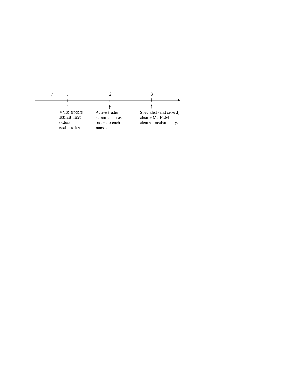
endogenous. A timeline of events is shown in Figure 1.

Liquidity is demanded by an active trader who arrives at time 2 and sub-

mits market orders to the two exchanges. The total number of shares x which
she trades is random and exogenous. With probability she wants to buy
and with probability 1

− she must sell. The distribution over the random

(unsigned) volume

x is a continuous strictly increasing function F . Since

the model is symmetric, we focus expositionally on trading when she must
buy x > 0 shares. As in Bernhardt and Hughson (1997), the active trader
minimizes her total trading cost by splitting her order across the two mar-
kets. In particular, let B

denote the number of shares she sends as a market

304

Liquidity-Based Competition for Order Flow

Figure 1
Timeline for sequence of events

buy to the hybrid market and let B

= x − B

be the market buy sent to the

pure market.

Liquidity is supplied by three types of investors. At time 1, competitive

risk-neutral value traders post limit orders in the pure and hybrid markets’
respective limit order books. At time 3, additional liquidity is provided by
trading crowds—competitive groups of dealers who stand ready to trade
whenever the profit in either market exceeds a hurdle level r . In addition, a
single strategic specialist with a cost advantage over both the value traders
and the crowd provides further liquidity on the hybrid market. All of the
liquidity providers have a common valuation v for the traded stock. Thus the
main issue is how much of a premium over v the active trader must pay for
immediacy so as to execute her trades.

Collectively the actions of the various liquidity providers—described in

greater detail below—lead to competing liquidity supply schedules, T

and

, in the two exchanges. In particular, T

is the cost of liquidity in

the hybrid market when buying B

shares (i.e., the premium in excess of

the shares’ underlying value vB

) and T

is the corresponding price

of liquidity in the pure limit order market. Given the two liquidity supply
schedules and the total number of shares x to be bought, the active trader
chooses market orders, B

and B

, to minimize her trading costs:

min

st B

+ T

(1)

Solving the active trader’s optimization [Problem (1)] for each possible

volume x > 0 lets us construct order submission policy functions, B

and B

x. These two policy functions, together with the distribution F over

x, induce endogenous probability distributions F

and F

over the arriv-

ing market orders B

and B

in the pure and hybrid markets and, hence,

over the random payoffs to liquidity providers. In equilibrium, the demand
for liquidity in the two markets, as given by F

and F

, and the liquid-

ity supply schedules, T

and T

, must be consistent with each other. One

goal of this article is to describe the equilibrium relation between the market
order arrival distributions and the liquidity supply schedules. What types of

305

The Review of Financial Studies / v 16 n 2 2003

market orders are sent to which markets? What do the limit order books and
liquidity supply schedules look like? How do regulatory linkages between
the two markets affect trading and liquidity provision? With this overview,
we now describe the model in greater detail.

1.1 Market environment
For simplicity, prices in both exchanges are assumed to lie on a common
discrete grid

= p

−1

. Prices are indexed by their ordinal

position above or below v, the liquidity providers’ current common valua-
tion of the stock. By taking v to be a constant, we abstract from the price
discovery/information aggregation function of markets and focus solely on
their liquidity provision role. Like Seppi (1997), this is a model of the tran-
sitory (rather than the permanent) component of prices.

If v itself is on

then it is indexed as p

. Since the active investor is willing to trade at a dis-

count/premium to v to achieve immediacy, she must have a private valuation
differing from v.

1.2 Limit orders and order execution mechanics
Limit orders play a central role—in our model as well as in actual markets—
both by providing liquidity directly and by inducing the hybrid market spe-
cialist to offer price improvement. Let S

denote the total limit sells

posted at prices p

in the hybrid market and let Q

h
j

j
i

be the

corresponding cumulative depths at or below p

. Define S

and Q

p
j

similarly for the pure market. All order quantities are unsigned (nonnegative)
volumes.

Investors incur up-front submission costs of c

per share when submitting

limit orders at price p

. We interpret these costs—which are ordered c

· · · at p

, p

—as a reduced form for any costs borne by investors

who precommit ex ante to provide liquidity such as, for example, the risk
of having their limit orders adversely “picked off” [see Copeland and Galai
(1983)].

Limit orders are protected by local priority rules in each exchange. In

the pure limit order market, price priority requires that all limit sells at
prices p

< p must be filled before any limit sells at p are executed. Given

price priority, a market buy B

is mechanically crossed against progressively

higher limit orders in the PLM book until a stop-out price p

is reached.

When executed, limit sells trade at their posted limit prices which may be
less than p

. At the stop-out price, time priority stipulates that if the available

limit and crowd orders at p

exceed the remaining (unexecuted) portion of

, then they are executed sequentially in order of submission time.

See Stoll (1989), Hasbrouck (1991, 1993), and Huang and Stoll (1997). Seppi (1997) shows that his analysis
carries over in a single market setting if v is a function of the arriving market orders, but that the algebraic
details are more cumbersome.

306

Liquidity-Based Competition for Order Flow

The hybrid market has its own local priority rules. When a market order B

arrives in the hybrid market, the specialist sets a cleanup price p

at which

he clears the market on his own account after first executing any orders with
priority. In addition to respecting time and price priority, the specialist is
also required by public priority to offer a better price than is available from
the unexecuted limit orders in the HM book or from the crowd. Thus, to
trade himself, the specialist must undercut both the crowd and the remaining
(unexecuted) HM limit order book.

The priority rules are local in that each exchange’s rules apply only to

orders on that exchange. The pure market is under no obligation to respect
the priority of limit orders in the hybrid book and vice versa. Priority rules
which apply globally across exchanges create, in effect, a single integrated
market. Section 3 explores the impact of cross-market priority rules.

1.3 The trading crowd
As part of the market-clearing process a passive trading crowd—a group of
competitive potential market makers/dealers with order processing costs of
r per share—provides unlimited liquidity by selling whenever p > v

+ r in

either market. We denote the lowest price above v

+r (the crowd’s reservation

asking price) as p

max

. This is an upper bound on the market-clearing price in

each exchange.

Our crowd represents both professional dealers at banks and brokerage

firms who regularly monitor trading in pure (electronic) limit order markets
as well as the actual trading crowd physically on the floor of hybrid markets
like the NYSE. In the pure market, we assume operationally that any excess
demand B

−

≤ p

max

> 0 that the PLM book cannot absorb is posted

as a limit buy at p

max

, where the crowd then sees it and enters to take the

other side of the trade. In the hybrid market, the specialist is first obligated
to announce his cleanup price p

and to give the crowd a chance to trade

ahead of him before clearing the market. Hence the specialist cannot ask
more than p

max

−1

(i.e., one tick below p

max

) and still undercut the trading

crowd on large trades.

1.4 The specialist’s order execution problem
The specialist has two advantages over other liquidity providers. First, he
has a timing advantage over the value traders. He provides liquidity ex post
(after seeing the realized size of the order B

), whereas limit orders, on both

markets, are costly ex ante precommitments of liquidity. Second, he has a
cost advantage over the trading crowd. Although we have singled out one
specific trader and labeled him the “specialist,” one could also view the mar-
ket makers/dealers in the crowd as having heterogeneous order processing
costs. All but one have costs r > 0, but one market maker/dealer has a com-
petitive advantage in that his order processing/inventory costs are zero. Our

307

The Review of Financial Studies / v 16 n 2 2003

specialist is simply whichever dealer currently happens to be the lowest-cost
liquidity provider in the market.

The specialist maximizes his profit from clearing the hybrid market by

choosing a cleanup price p

which, given the market order B

and the HM

book S

, solves

max

v < p

≤ p

max

−1

−

≤ p

− v

(2)

In particular, he sells at p

after first executing all HM limit orders with

priority.

The trade-off the specialist faces is that the higher the cleanup price,

the more limit orders have priority, and thus, the fewer shares he personally
sells at that price. The upper bound of p

max

−1

is because the specialist must

also undercut the HM crowd to trade.

In executing an arriving market order B

, the specialist competes directly

with the HM limit order book. Since he cannot profitably undercut limit
orders at p

(i.e., the lowest price above his valuation v), he simply crosses

small market orders, B

≤ S

, against the book and sets p

= p

. For larger

orders, B

> S

, the specialist sets the cleanup price p

so that he always

sells a positive amount.

This implies that hybrid limit orders S

at prices

> p

either execute in toto or not at all. In contrast, there is only partial

execution of any limit sells S

at p

when B

< S

From Seppi (1997) Proposition 1 we know that the specialist’s optimal

pricing strategy p

is monotone in the size of the arriving order B

Thus it can be described by a sequence of execution thresholds for order
sizes that trigger execution at successively higher prices

= max

< p

(3)

The cleanup price is p

≥ p

only when the arriving market order is suffi-

ciently large in that B

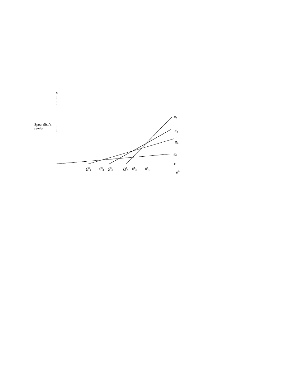
. Figure 2 illustrates this by plotting the special-

ist’s profit from selling at different hypothetical prices p

= p

max

−1

− Q

h
j

− v

(4)

conditional on different possible orders B

≥ Q

h
j

. Lemma 3 in Section 1.8 shows

that, in equilibrium, the execution thresholds

are determined, as shown here,

by the adjacent prices p

−1

and p

. When B

is less than

, the profit

−1

from

selling at p

−1

is greater than

, while for B

the profit

The specialist only trades once. Selling additional shares at prices below p

simply reduces the size of his

(more profitable) cleanup trade at p

. No submission costs c

are incurred on the specialist’s cleanup trade

since ex post liquidity cannot be picked off.

If p

= p

and B

> S

, then, by definition, the specialist is selling. If the specialist is not selling when

> p

, then he went “too far” into the book. Lowering p

would undercut some limit orders and thereby

let the specialist sell some himself at a profit.

308

Liquidity-Based Competition for Order Flow

Figure 2
Specialist profit maximization and hypothetical HM limit order depths and execution thresholds
Q

h
j

= cumulative depths in the HM limit order book,

= specialist’s profit from selling at price p

given a

market order B

> Q

h
j

, and

h
j

= execution threshold for price p

. This illustration assumes that Q

h
4

> Q

h
3

h
2

> 0, where p

= p

min

. To be consistent with Lemma 3 below, the thresholds are strictly ordered so that

h
j

at all prices p

with positive depth S

> 0.

greater than

−1

. When B

, the specialist is indifferent between selling

at p

−1

or p

. To ensure that the active trader’s Problem (1) is well defined

and has a solution, we assume that the specialist uses the lower of these
two prices and sets p

= p

−1

We summarize these properties in two

ways:

•

The largest market order that the active trader can submit such that the
specialist will undercut the HM book at p

by cleaning up at p

−1

. Orders larger than

are cleaned up at p

or higher.

•

For the value traders, their limit sells at p

> p

execute only if B

Implicit in the specialist’s maximization problem is the assumption that

the specialist takes the arriving order B

as given. In particular, he cannot

influence the active trader’s split between B

and B

by precommitting to

sell at prices which undercut the rival PLM market, but which are ex post
time inconsistent [i.e., do not satisfy Equation (2)]. This is equivalent to
assuming that the specialist only sees the arriving hybrid order B

(i.e., he

cannot condition on the actual PLM order B

) and that he has no cost advan-

tage in submitting limit orders of his own. With these assumptions, the only
role for the specialist is ex post (or supplementary) liquidity provision as in
Equation (2).

If p

h
j

= p

rather than p

−1

, then solving Problem (1) could involve trying to submit the largest order

such that B

h
j

in order to keep the HM cleanup price at p

−1

. Since this involves maximizing on an open

set, no solution exists. This assumption also justifies the “max” rather than a “sup” in Equation (3).

309

The Review of Financial Studies / v 16 n 2 2003

1.5 Value traders
We model value traders as a continuum of individually negligible, risk-neutral
Bertrand competitors. They arrive randomly at time 1, submit limit orders if
profitable, and then leave.

The depths S

and S

at any price p

in the two markets’ respective limit

order books are determined by the profitability of the marginal limit orders.
Each market’s book is open and publicly observable so that the expected
profit on additional limit orders can be readily calculated. In the HM book
the marginal expected profit on limit orders, given the specialist’s execution
thresholds, is

h
1

= Pr

≥ S

− v − c

at p

and

h
j

= Pr

− v − c

at p

(5)

where PrB

≥ S

and PrB

are the endogenous probabilities,

given the distribution F

, of a market order large enough to trigger execution

of all HM limit sells at prices p

or p

, respectively.

In the PLM book, the cumulative depths Q

p
j

play a role analogous to the

specialist’s execution thresholds in Equation (5). The marginal PLM limit
sell at p

is filled only if B

is large enough to reach that far into the book.

Thus the marginal expected profit at p

p
j

= Pr

≥ Q

p
j

− v − c

(6)

Value traders do not need to trade per se. They simply submit limit orders

until any expected profits in the PLM and HM limit order books are driven
away. Since limit order submission is costly, limit orders are only posted at
prices where there is a sufficiently high probability of profitable execution.
To derive a lower bound on the set of possible limit sells, we note that the
maximum expected profit at p

is p

−v−c

. This is the expected profit if

the limit order is always executed given any x > 0. From this it follows that
limit orders at prices where p

< v

are not profitable ex ante and hence

are never used. We denote the lowest price such that limit sells are potentially
profitable as p

min

= minp

∈ v +

< p

and note that p

> v

for

all prices p

> p

min

. Natural upper bounds are p

max

(in the pure limit order

market) and p

max

−1

(in the hybrid market) since the PLM crowd and HM

specialist undercut any limit sells above these prices. We make the following
simplifying assumption about the relative ordering of p

min

versus p

and p

max

in our analysis hereafter.

Unlike in the hybrid market, partial execution of limit sells above p

is possible in the PLM. However,

the resulting ex ante profitability of inframarginal PLM limit orders does not affect the profitability of the
marginal PLM limit orders and hence does not affect the equilibrium PLM depths S

310

Liquidity-Based Competition for Order Flow

Assumption 1. p

< p

min

≤ p

max

The assumption p

min

≤ p

max

means that positive depth in one or both of the

limit order books is possible. Otherwise the books would be empty. The
assumption p

min

> p

is the relevant case given the trend toward decimaliza-

tion and finer price grids.

An immediate implication of p

< p

min

is that now

the specialist always trades when a market order B

> 0 arrives. When the

arriving buy order is small, he always has the option of selling one “tick”
below the limit order book at p

min

−1

, thereby undercutting all of his rival

liquidity providers in the hybrid market.

1.6 The active trader
Our model differs from Seppi (1997) in that the active trader’s orders solve
an optimization problem. In particular, recall that the active trader chooses
her market orders B

≥ 0 and B

≥ 0 to minimize the total liquidity premium

she pays to buy x shares,

min

st B

= x

+ T

(7)

Given the actions of the liquidity providers described above, we now have
explicit expressions for T

and T

. In the hybrid market—given the HM

limit order book, S

min

, the associated thresholds

, and the crowd’s

reservation price p

max

—the active trader faces a cost schedule

≤ p

+ B

− Q

− B

(8)

where the first term is the cost of buying from the HM book and the second
is the cost of any shares bought from the specialist at his cleanup price,
p

. Recall that subtracting B

v simply expresses trading costs as a price

impact or liquidity premium in excess of the baseline valuation. In the pure
limit order market—given the PLM book S

min

and the crowd’s p

max

—the

active trader faces a liquidity cost schedule

< p

−

− B

(9)

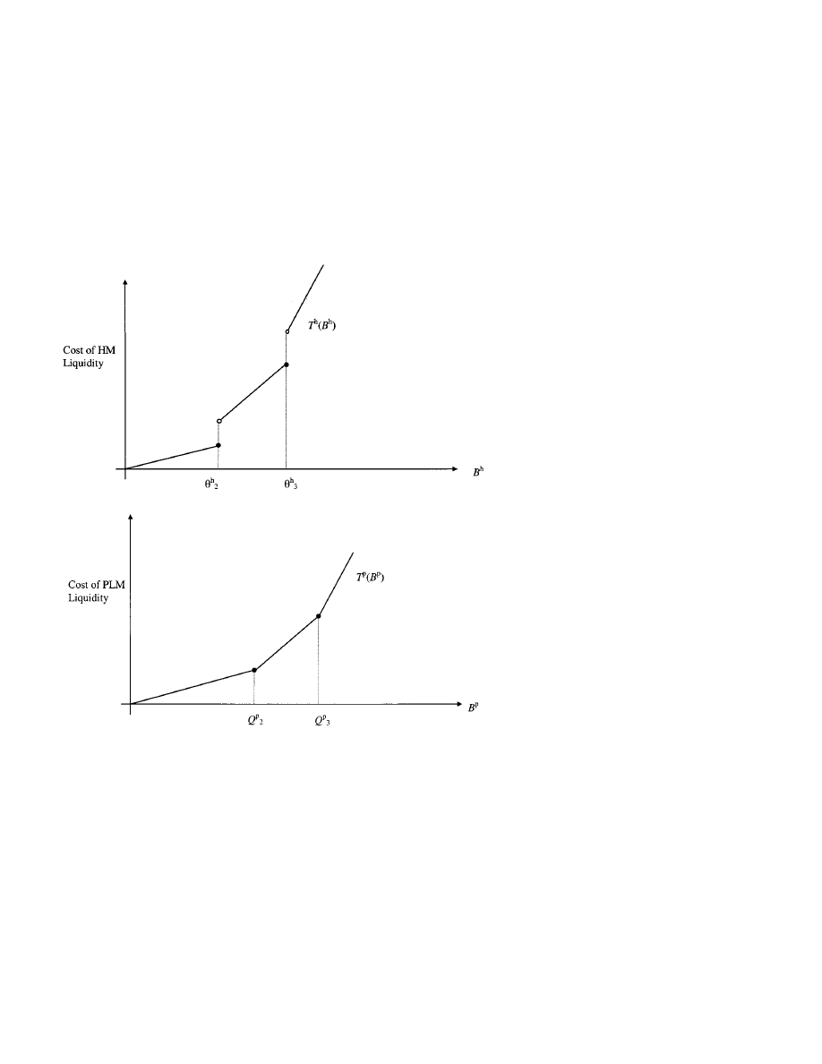
As illustrated in Figure 3, the two schedules differ significantly. In the

hybrid market, T

has discontinuities at each of the specialist’s thresholds

max

−1

, whereas T

in the pure market is continuous. The disconti-

nuities in T

arise because the specialist only provides liquidity at his cleanup

This assumption unclutters the statement of our results by eliminating a number of special cases at p

when

min

= p

. Since the specialist cannot profitably undercut the HM book at p

when S

> 0, limit sells at p

are different from limit sells at prices p

> p

. Details about the p

min

= p

case are available from the authors.

311

The Review of Financial Studies / v 16 n 2 2003

A: In the hybrid market

B: In the pure limit order market

Figure 3
Hypothetical liquidity cost schedules

price, p

. If B

, then the specialist crosses Q

h
j

−1

shares of the market

order with limit orders at prices p

min

−1

in the HM book and then

sells the rest,

− Q

h
j

−1

, himself at p

−1

. However, once B

exceeds

even a small > 0, the total cost of liquidity jumps, since undercutting the
limit sells at p

no longer maximizes the specialist’s profit. Now, after cross-

ing Q

h
j

−1

with the limit orders up through p

−1

, the remaining

+ − Q

h
j

−1

shares are executed at p

. Of this, S

comes from limit orders at p

and

+ −Q

h
j

is sold by the specialist. Thus when p

reaches p

, the specialist

stops selling at p

−1

, and there is a discrete reduction in the liquidity avail-

able at the now inframarginal price p

−1

. In contrast, a higher stop-out price

312

Liquidity-Based Competition for Order Flow

in the pure limit order market has no effect whatsoever on inframarginal

liquidity provision at lower prices in the PLM book.

An important fact about Equation (7) is that the active trader’s problem

may have multiple solutions for some x’s. This happens when the cost-
minimizing cleanup/stop-out prices are equal, p

= p

, and there is

some “slack” in the two liquidity supply schedules, x <

+ Q

p
j

. In this

case, small changes in B

and B

do not change p

and p

or the overall

total cost x and, as a result, the active trader is indifferent about where
she buys at p

. For total volumes x, where the solution to Equation (7) is

unique, the active trader’s orders, B

and B

, are entirely determined by cost

minimization. However, when multiple solutions exist, her choice of which
particular cost-minimizing pair of orders, B

and B

, to submit depends on

a “tie-breaking” order preferencing rule.

Definition 1. An order preferencing rule, , is a family of probability dis-

tributions

over the set of cost-minimizing orders B

and B

= x − B

solving Equation (7) indexed by the total volumes x.

The order preferencing rule , together with the distribution F over x, induce,
in turn, endogenous distributions F

and F

over the orders B

and B

arriving in the two markets. In practice, investors may preference one market
over another out of habit or because of “payment for order flow” or locational
convenience. While our notation allows for preferencing to be deterministic,
randomized, and/or contingent on the total volume x, this article focuses on
two polar cases in which either the pure or the hybrid market is consistently
preferenced.

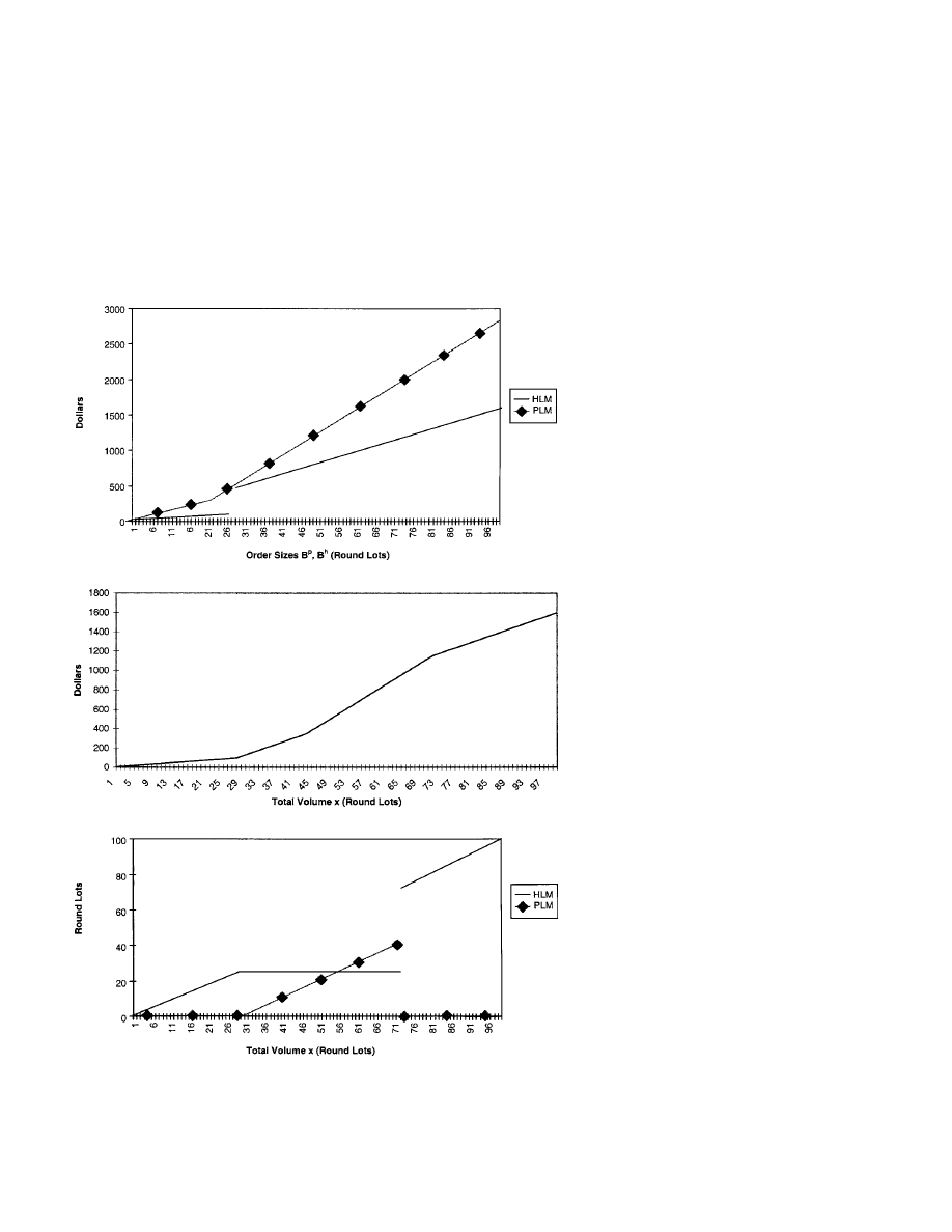
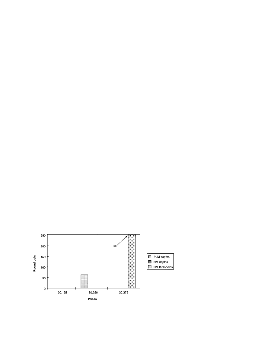
1.7 Numerical example
Figure 4 illustrates the choice of the active trader’s order submission strategy
B

x and B

x. In this example the active investor minimizes her total

trading costs given the two liquidity supply schedules T

and T

in Figure 4a,

where p

= $30125, p

= $3025, and p

= p

max

= $30375 and where the

stock’s common valuation is v

= $3009 per share. We show in Section 2 that

these particular schedules can be supported in equilibrium given a specific
order preferencing rule.

Figure 4b depicts the minimized aggregate cost schedule corresponding

to T

and T

and Figure 4c shows a pair of cost-minimizing order submis-

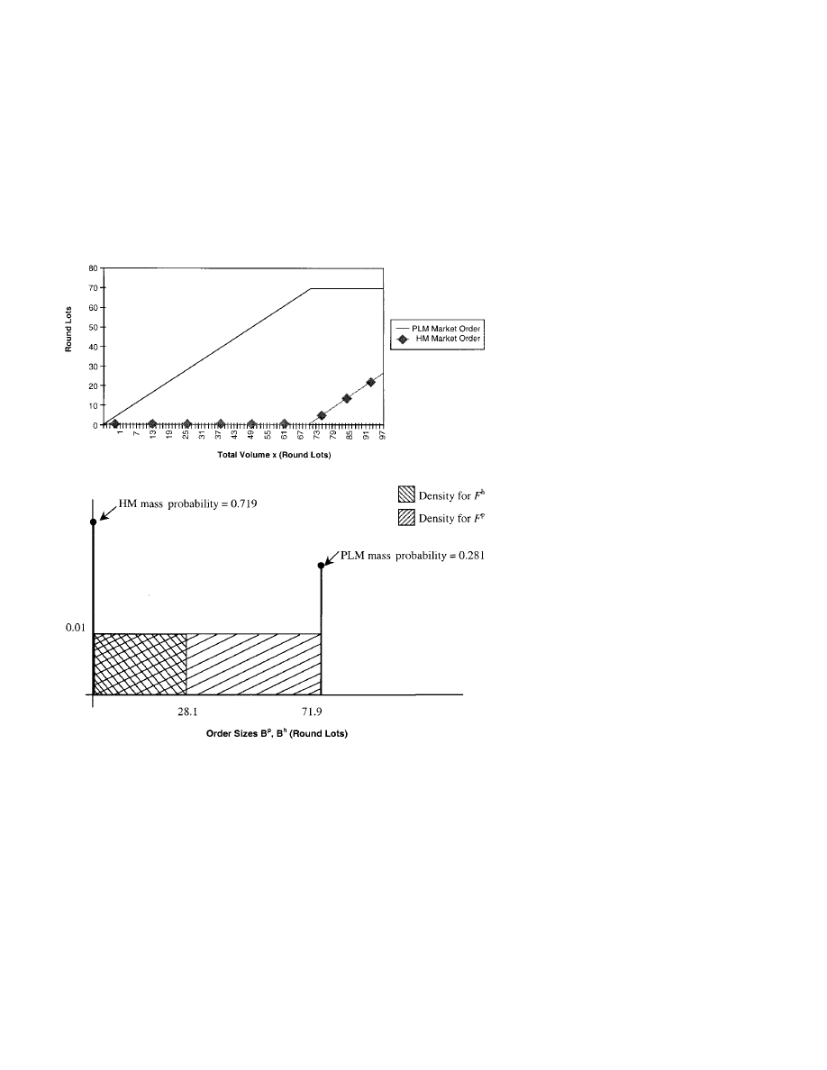
sion strategies B

x and B

x. If the active trader needs to buy x

≤ 281

round lots, then her costs are minimized by buying B

= x in the hybrid

market at a marginal cost of liquidity of p

− v = 0035 cents per share.

When 281 < x < 719 she optimally caps her order to the hybrid market at
B

= 281 (i.e., avoiding the discontinuity above 28.1) and buys B

= x−281

round lots in the pure market at a marginal cost of p

− v = 016 cents per

share (if B

≤ 156) or p

−v = 0285 cents thereafter (if 156 < B

< 438).

313

The Review of Financial Studies / v 16 n 2 2003

A: HM and PLM liquidity supply schedules

B: Minimized aggregate liquidity supply schedule

C: Optimal market order submissions

Figure 4
Example of optimal market order submission strategies and liquidity cost schedules
The numerical parameter values are the same as in Figure 8.

314

Liquidity-Based Competition for Order Flow

D: Endogenous HM and PLM order arrival densities corresponding to F

and F

Figure 4
(continued)

When x

≥ 719 her costs are minimized by any combination of orders B

≤

156 and B

= x − B

, since she is indifferent about where to buy the last

15.6 round lots (i.e., since the price is p

in either market). An order prefer-

encing rule is needed to pin down B

and B

in this region. In Figure 4c we

assume that, when indifferent, the active investor favors the hybrid market.
We consider this and other alternative preferencing rules in greater detail
below.

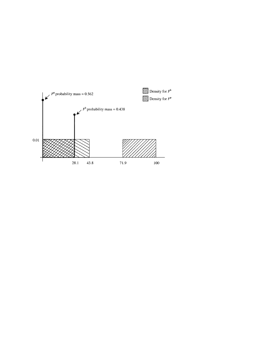
Figure 4d shows the densities corresponding to the order arrival distribu-

tions F

and F

induced by B

x and B

x given an additional assumption

that the total volume x is distributed uniformly over 0 100 round lots. As
this example illustrates, there can be endogenous “flat regions” (i.e., densities
equal to zero) and probability mass points in F

and F

even when the total

volume distribution F is continuous and increasing. In particular, the active
trader’s efforts to avoid the jump in the hybrid market liquidity supply sched-
ule T

leads to the mass point Pr281 < x < 719

= 0438 at B

= 281 in

and hybrid preferencing leads to the mass point Prx

≤ 281 + Prx ≥

719

= 0562 at B

= 0 in F

. The location of such mass points will play an

important role in the equilibrium interdependencies linking liquidity supply
(i.e., limit orders and the specialist’s cleanup decision) and liquidity demand
(i.e., the market order split).

1.8 Equilibrium
Given the market participants and their actions, an equilibrium is defined as
follows.

315

The Review of Financial Studies / v 16 n 2 2003

Definition 2. A Nash equilibrium is a set of depths, thresholds, and order

arrival distributions S

such that

•

The value traders’ marginal expected profit at each price p

in the pure

limit order book is nonpositive, e

p
j

≤ 0, if S

= 0 and zero, e

p
j

= 0, if

> 0.

•

Similarly, in the hybrid market e

h
j

≤ 0 if S

= 0 and e

h
j

= 0 if S

> 0.

•

The specialist’s execution thresholds

satisfy his profit maximiza-

tion condition [Equation (3)].

•

The market order arrival distributions F

and F

are consistent with the

active trader’s cost minimization problem [Equation (7)], the volume
distribution F , and a preferencing rule .

The endogeneity of F

and F

is critical to the definition and construction

of equilibrium in our model. As seen in Figure 4, the order arrival distri-
butions can be complicated with probability mass points and flat regions.
If F

and F

were exogenous, then competition might not drive expected

profits to zero since the limit order execution probabilities are not continu-
ous around exogenously fixed mass points. Indeed, Seppi (1997) shows that,
with fixed mass points in exogenous distributions F

and F

, the proper

competitive conditions (when depth is positive) are weak inequalities e

h
j

≥ 0

and e

p
j

≥ 0—rather than strict break-even conditions e

h
j

= 0 and e

p
j

= 0 as

above.

In our model, however, the location of any mass points is endogenously

determined by the active trader’s cost minimization problem [Equation (7)]
and her preferencing rule . Notice that, collectively, the value traders are
competitive first movers. Given the liquidity supply schedules T

and T

, the

active trader chooses B

and B

to minimize her trading costs. The schedule

is, in turn, determined by the submitted limit order book S

min

the pure limit order market. The hybrid schedule T

is determined by the

HM book S

min

both directly and also indirectly through the specialist’s

thresholds

. Thus the execution probability PrB

in the definition

of e

h
j

in Equation (5) depends on the depth S

both mechanically—in that

changing S

changes

, holding the distribution F

fixed—and, more fun-

damentally, in that changing S

changes the distribution of arriving market

orders F

itself via the impact of S

on T

and hence on the split between B

and B

. An analogous argument holds in the pure limit order market. In light

of the endogeneity of F

and F

, the execution probabilities in Equations (5)

and (6) can be written more explicitly as

PrB

= Pr

PrB

≥ Q

p
k

= Pr

≥ Q

p
k

(10)

Lemma 1. The limit order execution probabilities PrB

and PrB

≥

p
j

, and hence the marginal expected profits e

h
j

and e

p
j

are continuous func-

tions of S

and S

, respectively.

316

Liquidity-Based Competition for Order Flow

With continuous expected profits e

h
j

and e

p
j

, the competitive profit-seeking

behavior of the value traders ensures that expected profits are driven to zero
in equilibrium.

A number of insights follow directly from the break-even property of the

equilibrium limit order books. One of the most useful is that rewriting the
break-even condition e

p
j

= 0 using Equation (6) gives the equilibrium proba-

bilities of execution for the marginal PLM limit orders:

PrB

≥ Q

p
j

− v

at each p

≥ p

min

, where S

> 0

(11)

Similarly e

h
j

= 0 and Equation (5) give the equilibrium HM execution prob-

abilities:

PrB

− v

at each p

≥ p

min

, where S

> 0

(12)

The strong versus the weak inequalities in Equations (11) and (12) simply
reflect the difference in limit order execution in the two markets.

The key step when computing equilibria in Section 2 is to represent the

endogenous distributions F

and F

—from which the probabilities PrB

and PrB

≥ Q

p
j

are computed—in terms of the exogenous total volume

distribution F . Substituting these representations into Equations (11) and (12)
lets us solve for the equilibrium limit order books in the two markets. One
additional piece of notation will be useful when doing this. Let H denote
the inverse of the total volume distribution F , where Prx > H z

= z, and

define

−v

for p

= p

min

max

so that

−v

≤ 1

otherwise.

(13)

Since F is continuous and strictly increasing, the existence and uniqueness
of the H

’s is guaranteed.

Another implication of the limit order break-even property is that since the

specialist faces the same ex ante costs c

of having limit orders picked off as

do the value traders, and since the value traders compete away any expected
limit order profits, the specialist does not submit limit orders of his own.
In addition, the break-even property means that the HM book and execution
thresholds have the same simple structure in our model as in Seppi’s (1997)
Proposition 2. We restate this result here in two parts.

Our assumption that the value traders are individually negligible—that is, that they individually take the
aggregate depths S

and S

, and hence the distributions F

and F

as given—simplifies the definition of

equilibrium since it means we only need to check that the limit order books break even locally. In particular,
the profitability of noninfinitesimal deviations that change the depths S

and S

does not need to be checked.

317

The Review of Financial Studies / v 16 n 2 2003

Lemma 2. In the hybrid market, if S

> 0 and p

< p

max

, then S

> 0.

Lemma 3. In equilibrium the specialist’s execution thresholds are strictly

ordered

at prices with positive depth S

> 0 such that

= Q

h
j

−1

(14)

where

− p

−1

− v

(15)

Lemma 2 says that there are no “holes” in the HM book (e.g., positive depths
at p

−1

and p

, but S

= 0). Lemma 3 justifies the claim in Figure 2 that

the thresholds are determined by comparing the profits at adjacent prices.
The term

> 1 in Equation (14) measures how aggressively the special-

ist undercuts the hybrid limit order book at p

by selling at p

−1

2. Results About Competition

Jointly modeling the supply and demand of liquidity lets us investigate the
equilibrium impact of intermarket competition on both limit order placement
and the market order flow. As barriers to trade fall (e.g., with improved
telecommunications), a natural “feedback” loop seems to push toward a con-
centration of liquidity and trading. A market which attracts more market
orders will tend to attract more limit orders which, in turn, makes that mar-
ket more liquid and thus even more attractive to market orders.

On its face,

this might suggest that a single centralized market is the inevitable end state
for the financial marketplace.

Glosten (1994) predicts further that trading and liquidity will concentrate

in a single virtual competition-proof limit order market. The analysis lead-
ing to this prediction assumes, however, that the liquidity providers all face
identical costs and that the timing of their liquidity provision decisions is the
same (i.e., everyone must quote ex ante to participate). If, however, costs are
heterogeneous and if liquidity is both ex post and ex ante, is a centralized
marketplace still inevitable? Or is the coexistence of competing exchanges

Admati and Pfleiderer (1988) and Pagano (1989) were the first to study the concentration of order flow and
its connection with market liquidity.

318

Liquidity-Based Competition for Order Flow

possible? In answering these questions we focus particularly on the viability
of different markets’ respective limit order books.

Definition 3. The book in market I (either the HM or PLM) dominates the

book in the other market II if limit orders S

> 0 are posted at at least one

price p

in market I and if the limit order book in market II is empty, S

I I

= 0,

at each price p

, k

= 1 j

max

This criterion is weaker than competition-proofness in Glosten (1994) since
the specialist (or crowd) may still trade even when the hybrid (pure) book
is empty. If both books have positive depth, S

> 0 and S

> 0 at (possibly

different) prices p

and p

, we say the two markets coexist.

2.1 General results
Each of the two exchanges has distinct advantages relative to the other mar-
ket. On the one hand, the specialist has the lowest ex post cost of providing
liquidity. On the other, the continuity of the PLM liquidity supply schedule
T

makes the pure limit order market attractive for market orders.

Lemma 4. If the hybrid cleanup price is p

= p

> p

min

, then all PLM

limit sells at least up through p

−1

are executed in full, B

≥ Q

p
j

−1

, and thus

≥ p

−1

Lemma 5. The smallest total volume, infx

x >

, such that any

HM limit sells at p

> p

min

are executed in full is strictly larger than the

corresponding volume, infx

≥ Q

p
j

, for any PLM limit sells at p

The reason for the asymmetry between the two markets is that the HM

liquidity supply schedule T

is discontinuous at the execution thresholds

, whereas the PLM liquidity supply schedule T

is continuous. Thus if

and B

= Q

p
j

−1

for a volume x

+ Q

p
j

−1

, then, given a

slightly larger volume x

+ , the active trader always buys the additional

shares in the pure limit order market. Using the PLM as a buffer or “pressure
valve” in this way lets her keep B

and thereby avoid the discontinuous

jump in T

above

(as in Figure 3a). Indeed, since higher stop-out prices

increase only the slope of the PLM cost schedule T

(see Figure 3b), she

is even willing to buy a small number of shares at p

and potentially at

even higher prices in the PLM so as to keep the HM cleanup price at p

−1

It is this “pressure valve” role of the pure market that leads to Lemma 5.
Of course, once x is sufficiently large, it is cheaper to increase B

above

rather than to keep buying ever larger quantities x

−

−Q

p
j

at progressively

higher premia p

−p

indefinitely in the pure market. In doing so, the active

investor naturally scales back her premium PLM buying at prices p

319

The Review of Financial Studies / v 16 n 2 2003

Putting Lemmas 4 and 5 together does not imply that p

≥ p

. Cost min-

imization implies that, for some total volumes x, the marginal limit sell
at p

in the PLM book is optimally executed (i.e., B

≥ Q

p
j

) while the

marginal order in the HM book is unexecuted (i.e., B

≤

). However,

due to preferencing, the marginal HM limit sell at p

may execute when the

marginal PLM limit sell does not when the cost-minimizing split, B

and B

is not unique. Using this last observation, the probability of execution for the
marginal limit sell in the HM book can be written as

PrS

executes

= Prboth S

and S

execute

+ PrS

executes, but not S

due to preferencing

(16)

while the corresponding probability in the PLM book is

PrS

executes

= Prboth S

and S

execute

+ PrS

executes, but not S

due to preferencing

+ PrS

executes, but not S

due to cost

minimization

(17)

Thus the only way to support an equilibrium in which limit orders at p

the HM book coexist with (or dominate) limit sells in the PLM book—that
is, in which e

h
j

= 0 ≥ e

p
j

—is if the active trader’s preferencing rule favors

the hybrid market frequently enough in that

PrS

executes, but not S

due to preferencing

≥ PrS

executes, but not S

due to preferencing

+ PrS

executes, but not S

due to cost minimization

(18)

Hence the order preferencing rule plays a central role in supporting any
equilibrium with limit orders in the hybrid book.

2.2 Pure market order preferencing
An immediate implication of Inequality (18) is that if the active trader, when
indifferent, always preferences the pure limit order market over the hybrid
market, then the HM book is empty.

Definition 4. With pure market preferencing the active trader, when indif-

ferent, always sends the largest order B

to the pure limit order market such

that x

− B

solves Equation 7 for x.

Proposition 1. Given pure market preferencing, an equilibrium exists and

has a dominant PLM book (DPLM) where

320

Liquidity-Based Competition for Order Flow

•

The pure limit order book has positive depths at prices p

min

max

−1

given by

DPLM

= H

− H

−1

(19)

•

The hybrid limit order book is empty, S

= 0, at all p

, and

•

The active trader optimally splits her order, sending B

= minx H

max

−1

to the PLM and buying any residual, B

= max0 x −H

max

−1

, from the

specialist in the hybrid market.

Given an empty HM book, the active trader’s orders are directed first to

the pure limit order market, B

= x, until the available liquidity up through

max

−1

is exhausted. This lets us identify the endogenous probability of

execution PrB

≥ Q

p
j

with PLM preferencing as Prx

≥ Q

p
j

. Substitut-

ing this in Equation (11) and then recursively inverting using the identity
Q

p
j

= Q

p
j

−1

+ S

gives the equilibrium PLM book in Equation (19). Once

the active trader’s total volume is too large for the PLM limit order book
alone, x > Q

p
max

−1

= H

max

−1

, she caps B

at H

max

−1

and sends the rest,

= x − H

max

−1

, to the hybrid market where the specialist (given the empty

HM book) just undercuts the crowds’ p

max

by selling at p

max

−1

. Thus the

HM order arrival distribution F

has an endogenous mass point at B

= 0

equal to Prx

≤ H

max

−1

and F

has a mass point at B

= H

max

−1

equal to

Prx

≥ H

max

−1

. This is the unique equilibrium with pure market preferenc-

ing since, with a strictly increasing F , the H

’s are unique. Figure 5 is a

numerical example of this equilibrium.

The comparative statics for the equilibrium are intuitive. If the demand for

sell liquidity increases—that is, if the probability of a market buy order

A: A dominant PLM equilibrium with PLM preferencing

Figure 5
A dominant PLM equilibrium with PLM preferencing
Parameter values: common value v

= $30.09, ex ante limit order submission costs c

= $0.0263, c

= $0.0225,

= $0.0188, probability of a buy = 05, p

max

= $30.375, volume x uniform over [0, 100].

321

The Review of Financial Studies / v 16 n 2 2003

B: Optimal market orders B

in a DPLM equilibrium with PLM preferencing

C: Endogenous HM and PLM order arrival densities corresponding to F

and F

Figure 5
(continued)

increases or if the total volume distribution F shifts to the right in the sense
of first-degree stochastic dominance—then the cumulative depths Q

p
j

= H

are weakly larger. In other words, increased demand for liquidity induces,
in equilibrium, greater liquidity supply. The same is true if the limit order
submission costs c

decrease.

It may be surprising that the specialist—despite his status as the “lowest

cost” liquidity provider—is marginalized on all but the largest trades with
PLM preferencing. This outcome is a consequence of his inability to offer
credible price improvement when there are no HM limit orders to undercut.
Once a market order B

is in hand, the specialist has no incentive, given

the empty HM book, to offer any price improvement below p

max

−1

. We can

322

Liquidity-Based Competition for Order Flow

also show that alternative commitment mechanisms do not eliminate this
equilibrium.

One obvious mechanism for committing to offer price improvement would

seem to be for the specialist to post binding bid/ask quotes of his own.
Recall, however, that the specialist has no cost advantage in precommitting
to provide liquidity ex ante. Consequently any bid/ask quotes he might post
incur the same costs c

of being picked off as the value traders’ limit orders.

Since the DPLM limit order book is break-even, any HM quotes from the
specialist would trade at an expected loss after (given PLM preferencing) the
PLM limit sells. Thus the specialist cannot profitably use binding quotes to
attract market orders away from a competitive DPLM book.

If the specialist cannot precommit ex ante to provide price improvement,

why can’t the active trader use HM limit buy orders at price p

< p

max

−1

force price improvement from him ex post? We can show, however, that this
second mechanism also fails in the following sense:

Proposition 2. The DPLM equilibrium can be supported as a Bayesian

Nash equilibrium with beliefs that deter the use of limit buy orders above v
and below p

max

−1

by the active trader.

The key step in the proof is to notice that when the specialist sees a limit
order buy from the active trader, he does not know—given that he cannot see
x directly or infer it by seeing B

in the pure market—whether the active

trader is trying to bluff him into offering extra price improvement relative
to p

max

−1

. Giving him sufficiently suspicious beliefs supports HM limit buys

above v as off-equilibrium events.

On the surface, Proposition 1 is similar to Glosten’s (1994) competition-

proof result for pure limit order books. There are, however, two differences.
First, our specialist does provide superior residual liquidity on the “back end,”
x

−H

max

−1

, of large blocks by selling at p

max

−1

. This is because our liquidity

providers have heterogeneous costs—zero (ex post) for the specialist versus
c

(ex ante) for the value traders. Hence the PLM book is dominant but not

competition-proof. Second, other preferencing rules support other equilibria.
In particular, depending on how strongly the preferencing rule favors the
hybrid market, it is possible, from Inequality (18), to support equilibria in
which the HM and PLM books both coexist or even to have a dominant
hybrid book.

2.3 Hybrid market order preferencing
Having seen that pure market preferencing leads to a dominant PLM equi-
librium, it is natural to ask whether the polar opposite rule, hybrid market

One example of dealers’ vulnerability on this score is the evidence that lagging Nasdaq quotes are picked off
on the small order execution system (SOES) by SOES bandits. See Harris and Schultz (1998) and Foucault,
Roell, and Sandas (2003).

323

The Review of Financial Studies / v 16 n 2 2003

preferencing, is sufficient to offset the PLM’s cost minimization advantage
in Inequality (18).

Definition 5. With hybrid market preferencing, the active trader, when indif-

ferent, always sends the largest order B

to the hybrid market such that

− B

solves Equation (7) for x.

This is clearly the maximum possible preferencing of the hybrid market,

but even HM preferencing may be insufficient for HM dominance. In the
rest of this section we identify market parameterizations for which HM pref-
erencing leads to a dominant hybrid book when p

max

> p

We also show

that, outside of these parameter values, the two markets’ books coexist with
HM preferencing.

In a dominant HM equilibrium the PLM limit order book is, by definition,

empty. Consequently the active trader’s only alternative to the hybrid market
is buying at p

max

from the PLM crowd. Thus we start by asking: How large

must the total volume x be for the active trader to send an order B

the hybrid market if the PLM crowd is the only pressure valve?

Lemma 6. With HM preferencing, the market order B

submitted to the

hybrid market is weakly increasing in the total target volume x.

Lemma 7. In a dominant HM equilibrium, the active trader buys B

with a cleanup price p

≥ p

min

in the hybrid market when

≥ x ≥

≡ Q

h
j

−1

+ S

(20)

where

< 1 is given in Equation (15) and

max

− p

−1

max

− p

> 1

(21)

In the appendix we show that the critical volume x

is the solution to

≤ p

−1

− Q

h
j

−1

+ x −

max

≤ p

+ x − Q

h
j

(22)

The left-hand side of this equation is the cost, T

+ T

−

, of

buying B

in the hybrid market (so as to keep p

= p

−1

) and buy-

ing the rest at p

max

in the pure market. The right-hand side is the cost,

+ T

0, of buying everything in the hybrid market and accepting the

Given the restriction in Assumption 1, the only other possibility is p

max

= p

min

, in which case both the

HM and the PLM books are empty since the specialist provides unlimited liquidity at p

max

−1

= p

324

Liquidity-Based Competition for Order Flow

higher cleanup price p

= p

. When x

the active investor is indifferent

between these two alternatives so that, given HM preferencing, B

and B

= 0. The restriction

≥

in Inequality (20) simply ensures

that the specialist is, in fact, willing to clean up at p

The term

is a measure of the relative cost of using the PLM crowd as

a pressure valve to avoid raising B

above

. Fix, for example, a particular

price p

and then let the cost of trading with the crowd increase without

bound, p

max

→ . We see that

→ 1 and

→

. Thus the active trader

diverts less of her trading to the PLM as the cost of the pressure valve
increases.

We use Lemmas 6 and 7 to express the endogenous execution probability

PrB

as the probability Prx

≥

. Substituting this into the break-

even condition of Equation (12) and inverting gives

= H

(23)

which then, using Equation (20), can be recursively rearranged to get the
HM limit order book when a dominant HM equilibrium exists.

Lemma 8. In a dominant HM (DHM) equilibrium the break-even HM book

DHM

for p

< p

min

− Q

DHM
j

−1

for p

= p

min

max

−1

(24)

The term

< 1 describes how the active trader’s strategic use of the PLM

crowd as a pressure valve thins out the HM limit order book. Similarly

< 1

describes the negative impact of strategic undercutting by the specialist on
the HM book.

Lemma 8 characterizes the dominant HM book provided that a dominant

HM equilibrium in fact exists. HM preferencing alone is not, however, suf-
ficient to guarantee a dominant HM equilibrium. Existence hinges on two
conditions.

Condition 1. The specialist must be willing, as noted in Inequality (20), to

sell

− Q

h
j

shares at p

in that

≤

Condition 2. Value traders do not want to post limit orders in the PLM

book. This means that e

p
j

≤ 0 given the hybrid depths S

DHM

from Lemma 8

and an otherwise empty PLM book.

Consider the specialist’s willingness to trade first. Condition 1 is always satis-

fied at p

max

−1

(since

max

−1

max

= ), so consider prices p

min

max

−2

325

The Review of Financial Studies / v 16 n 2 2003

Substituting Equation (24) into Equation (14) gives the dominant HM exe-
cution thresholds

DHM

= M

≡

−

≤ i ≤ j−1

+1 < k ≤ j

−

(25)

in terms of the total volume distribution parameters H

, H

. Using this

expression for

we can formalize Condition 1 as a restriction on the

volume distribution F .

Lemma 9. A necessary condition for a dominant HM equilibrium with HM

preferencing is that at each price p

= p

min

max

−2

≤ M

(26)

so that

≤

DHM

and thus p

= p

Next, consider Condition 2 for PLM profitability condition. For the pure

limit book to be empty, the expected marginal profit on PLM limit sells must
be e

p
j

≤ 0 when S

= · · · = S

max

= 0 given the hybrid book in Lemma 8

and the corresponding

’s and

DHM

’s in Equations (23) and (25). This

is best understood in terms of limit order execution probabilities. Consider
an infinitesimally small PLM limit sell S

= at a price p

< p

max

. Only

infinitesimal deviations need to be considered since value traders are individ-
ually negligible. As illustrated in Figure 6, the limiting execution probability
lim

→0

PrB

> given an otherwise empty PLM book is the sum of the

probabilities that is used as a pressure valve—that is, when the total volume
x is in an interval

DHM

for some price p

≤ p

—plus the probability

that x >

so that both the HM and the hypothetical PLM limit sells at

execute. In contrast, the probability that the marginal HM limit order exe-

cutes is simply the probability that x

≥

. Differencing the two probabilities

gives another restriction on the volume distribution F :

Lemma 10. A second necessary condition for a dominant HM equilibrium

with HM preferencing is

PrH

≤ x ≤ M

−

≤p

PrM

< x < H

≥ 0

(27)

at prices p

= p

min

max

−2

and

max

− v

≥

≤p

max

−1

PrM

< x < H

(28)

Only one restriction, Inequality (28), is needed for both p

max

−1

and p

max

. Since

the hypothetical execution probability at p

max

is the same as at p

max

−1

—both

326

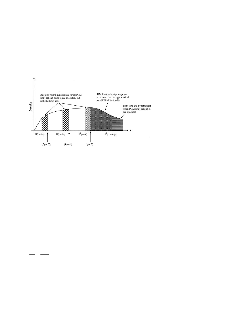
Liquidity-Based Competition for Order Flow

Figure 6
Regions for PLM and HM marginal limit order execution at price p

with HM preferencing

limit orders only execute in their pressure valve roles given HM preferencing—
if PLM limit orders at p

max

are not profitable, then neither are those at p

max

−1

In addition to being necessary, Lemmas 9 and 10 are also, by construction,

sufficient for a dominant HM equilibrium.

Proposition 3. Any continuous, strictly increasing distribution F which sat-

isfies Lemmas 9 and 10 supports a dominant hybrid market equilibrium.

We denote the set of distributions that satisfy Conditions 1 and 2 for a

given market environment

= c

min

r as

. The quantities H

and M

implicitly describe key features of the distribution of the random

demand for liquidity F . However, what do these distributions look like more
intuitively? And do such distributions exist for any environment ?

When p

max

> p

min

≥ p

, we can always find some volume distributions

which satisfy Conditions 1 and 2. First, F must be skewed enough to make
each of the M

’s (weighted averages of the H

’s and lower H

’s) larger

than the H

’s as required by Lemma 9. Second, we need enough “clustering”

to ensure that the conditions in Lemma 10 hold. In particular, although the
overall probability PrH

≤ x < H

in each interval H

is fixed at

−v

−

−v

by Equation (13), we need a sufficiently large probability in

the bottom subintervals H

and a sufficiently small probability in the

corresponding top subintervals M

to satisfy Lemma 10. From the

preceding discussion it follows that

is nonempty.

Figure 7a illustrates a dominant HM equilibrium. The parameterization

is the same as in Figures 4 and 5 with one difference. As illustrated in
Figure 7b, the distribution F here differs from the previous uniform 0 100

327

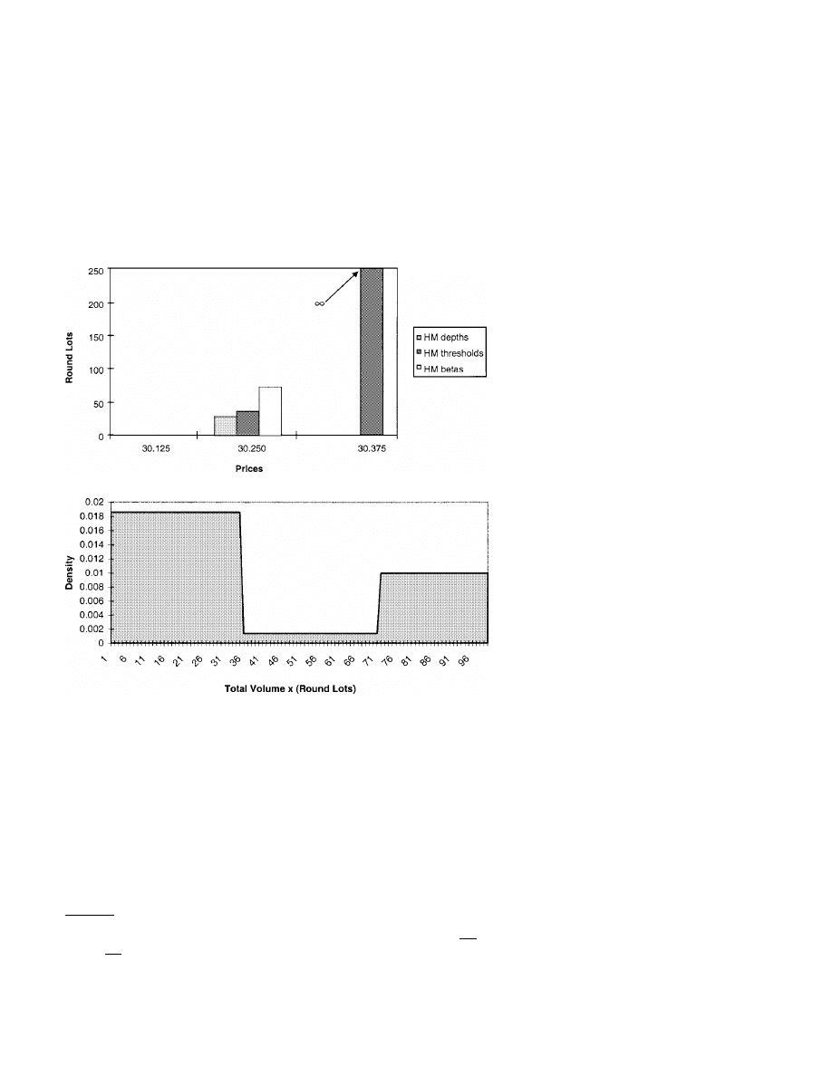
The Review of Financial Studies / v 16 n 2 2003

A: DHM depths, thresholds, and betas

B: Total volume density supporting a DHM with HM preferencing

Figure 7
A dominant hybrid market equilibrium with HM preferencing
Parameter values: common value v

= $30.09, ex ante limit order submission costs c

= $0.0263, c

= $0.0225,

= $0.0188, probability of a buy = 05, and p

max

= $30.375. The parameters are the same as in the other

examples except that the total volume distribution F in Figure 7B is not uniform.

distribution in that the probability Pr0 < x

≤ M

= 359 is increased to 67%

to offset a reduction in the probability PrM

< x < H

= 719 to 5%. This

is an example of the probability clustering described in Lemma 10.

The

execution threshold

for hybrid limit sells at $30.25 is roughly 35.9 round

lots. As Figures 7c and 7d illustrate, for volumes between

and

= 719

With a uniform distribution for total volume, the execution probabilities for infinitesimal PLM limit orders at
p

and p

are both PrM

< x < H

= 36% which exceeds their respective break-even probabilities

c2/

p2−v

28% and

c3/

p3−v

= 13%. The violation of Condition 2 in the uniform example is not caused by the uniform

distribution per se, but rather by this combination of parameters taken together. For example, if is reduced
to 25%, then the uniform distribution does support a DHM equilibrium.

328

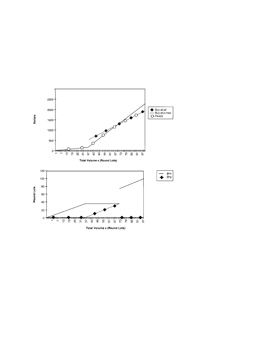
Liquidity-Based Competition for Order Flow

C: DHM active trader costs

D: DHM active trader optimal market orders

Figure 7
(continued)

round lots the cost T

−

of using the PLM crowd as a pressure

valve is less than the cost of buying the full x shares outright in the hybrid
market. Thus in the interval 359 719, the hybrid order B

is constant at

35.9 round lots which, in turn, implies that the specialist’s profit over this
region is constant at $125.8 and that the active trader’s total cost schedule
x has a steep slope equal to p

max

− v = $0285. Above 71.9 round lots,

however, it is cheaper to buy the whole x shares in the HM. At this point the
slope of the active trader’s cost schedule x falls from p

− v to p

− v =

$016 and the specialist’s profit jumps discontinuously and then is (once
again) increasing in x.

The comparative statics for local changes in , r , and c

—that is, for

which F is still in the new set

—are again intuitive. Increased demand

for sell liquidity and lower submission costs lead to a deeper DHM book
and greater aggregate liquidity. Unfortunately comparative statics for the set

329

The Review of Financial Studies / v 16 n 2 2003

itself are ambiguous since changing , r , and c

involves checking the

conditions in Lemmas 9 and 10 for different regions of the distribution F .
We do have a comparative static result for changes in the common price grid
when the tick size is a constant p

− p

−1

= .

Proposition 4. Holding the distribution F and the rest of the market envi-

ronment fixed, it is not possible to support a DHM equilibrium if the tick
size is too small.

One implication of this result is that the recent move to decimal pricing in
the United States may erode the dominance of the (hybrid) NYSE in equity
trading in the future. Holthausen, Leftwich, and Mayers (1987) and others
estimate that the transitory premium/discount on block trades, a natural proxy
for p

max

− v, was rarely more than a couple of ticks before decimalization.

This suggests that a DHM equilibrium was quite natural then, since Condi-
tions 1 and 2 are easier to satisfy on a coarse price grid. However, in the new
postdecimalization regime, with much finer price grids, this may no longer
be true.

Having shown that pure limit order markets are not exclusively competition-

proof when F

∈

, we next show that liquidity need not concentrate in a

single market. In particular, coexistence of competing pure and hybrid books
is also possible.

Proposition 5. If p

max

> p

min

, then hybrid preferencing leads to coexistence

of both the PLM and HM limit order books for distributions F

∈

Coexistence equilibria with HM preferencing can be computed recursively
in the special case where p

max

= p

. Using our maintained assumption that

min

> p

and thus S

= S

= 0, we solve the equation T

+ T

−

at p

in the hybrid market to get the critical value

+ S

(29)

and then invert PrB

= Prx ≥

−v

to get the hybrid depth and

the associated execution threshold

= H

− S

and

− S

(30)

Given HM preferencing and p

max

−1

= p

, the active trader buys everything

in the hybrid market (i.e., B

= 0) once x ≥

= H

. Thus the PLM depth

at p

(if nonnegative) can be computed numerically from

PrB

≥ Q

p
2

= Pr

+ Q

p
2

− S

+ S

≤ x < H

− v

(31)

330

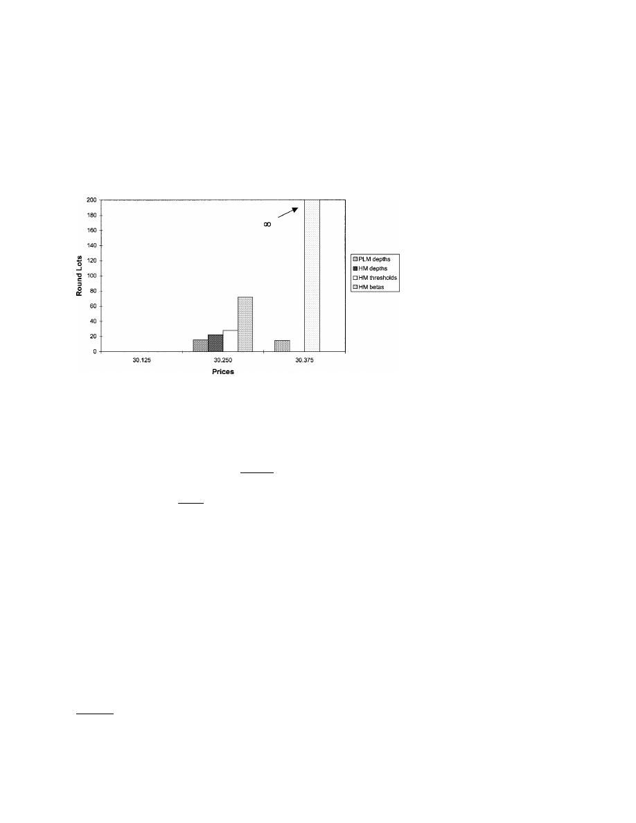
Liquidity-Based Competition for Order Flow

Figure 8
Example of coexistence with HM preferencing
Parameter values: common value v

= $30.09, ex ante limit order submission costs c

= $0.0263, c

= $0.0225,

= $0.0188, probability of a buy = 05, p

max

= $30.375, volume x uniform over [0, 100]. See Figure 4

for strategies, cost schedules, and order arrival distributions.

Given the solution for S

, we then compute S

at p

from

PrB

≥ Q

p
3

= Pr

+ Q

p
3

− S

+ S

≤ x < H

− v

(32)

Figure 8 gives the limit order books and thresholds for the numerical

example of coexistence illustrated earlier in Figure 4. Since Condition 2 is
not satisfied for a uniform distribution F and these parameters (see note 16),
both limit order books have positive depths. These books and the specialist’s
optimal response lead, in turn, to the equilibrium liquidity supply schedules
depicted in Figure 4.

Unfortunately when p

max

> p

, the equilibrium with HM preferencing can-

not be constructed recursively when F is not in

. This is because the pos-

sibility of positive depths at higher prices in the PLM book now affects the
profitability of limit sells at lower prices.

2.4 Other preferencing rules
The two extreme rules considered here highlight the range of possible equi-
librium allocations of liquidity and trading across the pure and hybrid mar-
kets. Clearly many other preferencing rules—for example, with deterministic

None of this changes the fact that, with PLM preferencing, a dominant PLM equilibrium always exists and
can be calculated recursively as above. Similarly, as long as F

∈

, a dominant HM equilibrium with HM

preferencing also exists and can still be calculated recursively. Nonrecursivity is only an issue outside of these
cases.

331

The Review of Financial Studies / v 16 n 2 2003

or x-contingent pro rata sharing and/or randomization—are also possible.
Without analyzing the details of such alternatives, we make a few general
observations. First, two preferencing rules which differ only in the partial exe-
cution of inframarginal limit orders in the PLM book have the same marginal
break-even conditions e

p
j

≤ 0 and e

h
j

≤ 0, and hence the identical equilibrium

depths. Second, preferencing rules which are intermediate between HM and
PLM preferencing should have intermediate equilibrium depths. Thus many
of these intermediate preferencing rules will also support coexistence of the
pure and hybrid limit order books.

3. Comparisons with Other Trading Architectures

When regulators decide whether to permit new trading venues to open, they
are, naturally, concerned about the possible fragmentation of order flow and
any impact it might have on aggregate liquidity. Corporations have similar
concerns in deciding whether to cross-list their stock in multiple markets.
Easley, Kiefer, and O’Hara (1996) and Battalio and Holden (1996) focus on
price discovery and intermarket “cream skimming,” whereas we focus on the
impact of intermarket competition on aggregate liquidity. We consider sev-
eral alternative institutional arrangements and compare the resulting liquidity
supply and trading outcomes. We find significant differences depending on
the institutional arrangement of the market. Table 1 summarizes the results
discussed below.

3.1 Competition versus a single hybrid market
Consider a stock which initially trades on just the NYSE (i.e., a hybrid
market). Would the opening of an ECN (i.e., a pure limit order market)
improve aggregate liquidity?

Before the ECN opens the active trader has no choice about where to trade

and hence B

= x. This leads to the single hybrid market (SHM) equilibrium

Table 1
Welfare comparisons across equilibria for active traders with different total volumes

Pairing

Small volumes

Mid-size volumes

Large volumes

SPLM
versus

Indifferent

DPLM

SHM
versus

Indifferent

SHM

DHM

SHM (or DHM)
versus

SHM (or DHM)

Ambiguous

DPLM

SPLM
versus

DHM

Ambiguous

DHM

332

Liquidity-Based Competition for Order Flow

from Seppi (1997) in which the hybrid book and corresponding execution
thresholds are given by

SHM

= H

− Q

SHM
j

−1

at prices p

= p

min

max

−1

(33)

SHM

at prices p

= p

min

max

−1

at p

max

(34)

Who wins and loses after the ECN opens depends on which competitive

equilibrium prevails. If a dominant HM equilibrium prevails, then small retail
investors (with small x’s) are indifferent while medium and large institutional
investors (for whom x is larger) are worse off. In both the SHM and DHM
equilibria the specialist provides liquidity at p

min

−1

on small orders and at

max

−1

on very large orders, but the DHM limit order book is less deep than

the SHM book. In particular, comparing the depths in Equation (24) with the
S

SHM

’s leads to the following:

Proposition 6. For every F

∈

, the cumulative single HM depth Q

SHM
j

each price p

≥ p

min

is greater than the corresponding depth Q

DHM
j

in the

dominant HM equilibrium.

Intermarket competition and the resulting order flow fragmentation actually

reduce aggregate liquidity in this case. The first reason is that the lower
cumulative depth in the DHM book reduces the inframarginal liquidity from
limit orders at prices below p

when x >

min

= H

min

. The second is that

when

DHM

= M

< x < H

DHM
j

SHM

, the active trader pays p

max

(in

the pure market) on her last x

−M

shares in the DHM equilibrium, whereas

she pays no more than p

−1

in the SHM equilibrium. Thus, although using

the PLM crowd as a pressure valve reduces the active trader’s cost taking
the HM book as given, once the equilibrium effect on the endogenous depths
is included—that is, after taking into account the response of value traders
who rationally anticipate lower HM limit order execution probabilities due
to order flow fragmentation—the DHM equilibrium has higher trading costs.

A dominant HM equilibrium is not the only possible competitive outcome.

If a dominant PLM equilibrium prevails instead (i.e., if the ECN attracts all of
the limit orders and most of the market order flow), then the comparison with
the single HM equilibrium is ambiguous. Large traders, with x > H

max

−1

, now

prefer competition and the dominant PLM equilibrium since the maximum
cleanup prices are the same (i.e., p

max

−1

) and the DPLM book is deeper (i.e.,

SHM
j

SHM

= H

= Q

DPLM
j

). In contrast, small retail investors, for whom

x < H

min

, strictly prefer a single HM (or the DHM) equilibrium because of

the intraspread price improvement the specialist provides to undercut the HM
book at p

min

> p

on small trades. This is not a minor consideration. Ross,

Shapiro, and Smith (1996) find that intraspread execution by the specialist
accounts for one-quarter of the price improvement on the NYSE. Barclay,

333

The Review of Financial Studies / v 16 n 2 2003

Hendershott, and McCormick (2001) also find lower price impact costs on
small dealer-executed trades than on small ECN trades on the Nasdaq.

3.2 Competition versus a single pure limit order market
Now consider the entry of a hybrid market when the stock is initially listed
only on a pure limit order market. Once again, there are a multiplicity of
possible post-entry competitive equilibria depending on the preferencing rule.
The trick with this comparison, however, is to describe the correct initial
equilibrium with the pure limit order market alone. In addition to the active
trader, value traders, and the PLM trading crowd, there is also the person
who would otherwise be the HM specialist to consider.

We consider the simplest case by assuming that the specialist’s cost advan-

tage derives entirely from his privileged institutional position in the hybrid
market.

Thus, in a single PLM setting without these institutional advan-

tages, he is just another dealer in the crowd with costs r . In this case,
Seppi’s (1997) SPLM equilibrium—in which B

= x and S

SPLM

= H

− H

−1

up through p

max

(i.e., rather than just p

max

−1

as in the DPLM)—is the cor-

rect pre-entry reference point. If a DHM equilibrium prevails after the hybrid
market enters, then the comparison with the SPLM is ambiguous. Very small
and very large investors prefer the DHM since they value the price improve-
ment from the specialist on small trades (undercutting the book at p

min

−1

)

and on large trades (undercutting the crowd at p

max

−1

). Intermediate investors

benefit from the deeper limit order book in the SPLM. If instead a DPLM
equilibrium prevails after the hybrid market enters, then aggregate liquidity
is unambiguously better. In particular, liquidity is unchanged for small and
midsize orders (since the SPLM and DPLM books are identical up through
p

max

−1

) and liquidity is strictly better in the DPLM for large trades (since

the specialist again provides infinite liquidity at p

max

−1

3.3 Liquidity providers’ welfare
One reason to focus on the cost of liquidity to the active trader is that liquid-
ity is empirically observable. This is not, however, to say that the liquidity
providers’ welfare is unimportant. One immediate implication of our analysis
is that value traders are better off in equilibria in which limit orders are placed
in the PLM book (e.g., SPLM, DPLM, and coexistence) than in equilibria
in which limit orders are posted only in the HM book (e.g., the SHM and
DHM). Although the marginal limit orders just break even in either market,
the inframarginal limit orders at prices p

> p

earn positive expected profits

in the pure limit order market due to the possibility of partial execution. In
contrast, recall that limit orders at p

> p

in the hybrid market are either

executed in toto or not at all. Thus there is no profitable inframarginal HM
order execution above p

. Conversely the specialist clearly trades more and

is thus better off in the SHM and DHM equilibria than in the DPLM.

Details about comparisons with other pre-entry assumptions are available from the authors.

334

Liquidity-Based Competition for Order Flow

3.4 Endogenizing the total trading volume
One caveat about our welfare comparisons is that the total volume distribu-
tion F is exogenous. Ideally the demand for liquidity x and its distribution
F should be modeled as functions of the prevailing liquidity supply sched-
ules T

and T

. In particular, discontinuities (as in the SHM equilibrium)

and nonconvexities (as in the DHM equilibrium) in the aggregate liquidity
supply schedule x mean that active traders with any discretion in their
total trading needs will sometimes curtail their trading in order to optimize
the trade-off between trading costs and the amount traded (e.g., to avoid a
discontinuity). We leave this important topic for future work.

3.5 “Best execution” regulations
When exchanges compete under a common regulatory umbrella, such as two
markets in the same country, regulators can and do impose cross-exchange
“best execution” restrictions on pricing [see Macey and O’Hara (1997)]. The
creation of the National Market System in 1975 and the 1996 SEC “order
handling” rules protecting customer limit orders on the Nasdaq are two such
examples. More recently the controversy over a centralized limit order book
was, in part, a debate about whether to impose cross-market time priority
and whether to permit ex post price improvement by specialists [see Levitt
(2000) and NYSE (2000)]. Such regulatory interventions directly affect the
incentives of liquidity providers. We study these issues by varying the insti-
tutional environment and seeing how this affects the behavior of our four
types of investors.

If price, time, and public order priority are imposed uniformly across all

exchanges, then the result is a single integrated market. In our model, with a
specialist, this leads to the SHM equilibrium. Our intent here is to explore less
sweeping cross-market regulations between the polar cases of unregulated
competition (as in Section 2) and a de facto single integrated market.

A natural intermediate case to consider is one in which price priority

applies globally across markets, but where time and public order priority are
still local. One way to model such a regime is to view global price priority
as a constraint on order execution. In particular, if the specialist wants to
clean up at p

when B

< Q

p
j

−1

, then he must first redirect Q

p
j

−1

− B

from B

over to the PLM to clean up the unexecuted limit sells through

−1

. The PLM limit sells at p

, however, may stay unfilled. Similarly the

PLM order execution system must divert orders to the hybrid market if there
are unexecuted HM limit orders at p

−1

once all of the PLM limit sells at

−1

are exhausted. Unfortunately, while such a representation is realistic, it

quickly leads to dynamic interactions between the two markets which are
beyond our static model. To avoid these complications we instead impose
global price priority as a constraint on the active trader’s order submission
problem.

335

The Review of Financial Studies / v 16 n 2 2003

Definition 6. Global price priority requires the active trader to submit orders,

and B

, such that the corresponding market clearing prices, p

and

, are no more than one “tick” apart. Thus, given ordered thresholds and

depths

and Q

p
j

−1

≤ Q

p
j

, the orders B

and B

must jointly satisfy

< B

≤

and Q

p
j

−1

≤ B

≤ Q

p
j

Giving price priority to the PLM limit orders vis-à-vis the HM specialist

has little practical “bite.” Recall from Lemma 4 that, even without such a
constraint, the optimal PLM order is B

≥ Q

p
j

−1

when p

= p

. Applying

global price priority in the other direction, however, dramatically curtails the
PLM’s pressure valve role. In particular, the active trader can no longer buy
at p

≥ p

in the PLM so as to keep the specialist at p

= p

, since doing

so would leave the HM limit sells at p

unfilled. In this direction, global

price priority does have some “bite.”

Proposition 7. Given global price priority across markets, hybrid market

preferencing leads to a single hybrid market (SHM) equilibrium.

Proposition 8. Multiple equilibria can be supported with PLM preferencing

and global price priority in that the two markets’ books can be either (a) the
dominant PLM equilibrium books with S

= S

DPLM

and S

= 0 or (b) any

set of nonnegative HM depths S

max

−1

and the corresponding PLM

depths S

max

−1

satisfying

+ S

= H

− Q

h
j

−1

− Q

p
j

−1

(35)

−1

− 1

−1

(36)

The net effect of global price priority is a dramatic improvement in the

competitive viability of hybrid markets regardless of the preferencing rule.
Proposition 7 shows that an SHM equilibrium can now be sustained for any
distribution F rather than just those in

. Even with PLM preferencing,

Proposition 8 shows that equilibria with positive depths in the HM book—
including an SHM equilibrium—are now possible in addition to the DPLM
equilibrium.

4. Conclusion

We have modeled liquidity-based competition for market and limit order
flow in an environment in which liquidity providers have heterogeneous
costs. Multiple equilibria exist, depending on the preferencing rule used by
investors to decide, when indifferent, where to route their market orders.
Some of the equilibria involve coexistence of competing exchanges while
others have concentrated trading and liquidity on a single exchange. Small

336

Liquidity-Based Competition for Order Flow

“tie-breakers” such as “payment for order flow,” habits, etc., can have a
significant impact on equilibrium selection. We also show that “best execu-
tion” regulations such as global price priority have real “bite” in that they
prevent cross-market marginal price differences of two ticks or more. This
reduces the ability of a pure limit order market to act as a pressure valve,
thereby dramatically increasing the competitive viability of a hybrid limit
order/specialist market. We see many promising directions for future work.
These include

•

Characterizing the relationship between preferencing and the robustness
of coexistence versus dominant market equilibria more systematically.
We have only considered two polar extremes.

•

Introducing asymmetries across markets such as different ex ante limit
order submission costs c

, crowd reservation profit levels r , or tick sizes.

Letting markets independently choose their own price grids would be
particularly interesting.

•

Adding exchange-specific clienteles of investors who have different rel-
ative costs for submitting limit and/or market orders on the competing
exchanges.

•

Endogenizing the total volume distribution F to allow for a trade-off
between trading costs and the total number of shares traded.

Appendix

Proof of Lemma 1.

This follows from the continuity of F together with the continuity of T

in S

(i.e., since the thresholds

are continuous in the HM depths), the continuity of T

in S

and thus the respective continuity of B

and B

Proof of Lemmas 2 and 3.

These follow from the same logic as Seppi’s (1997) Proposition 2,

given that the equilibrium HM book satisfies a break-even condition e

h
j

= 0 at each price with

positive depth S

> 0.

Proof of Lemma 4.

Consider p

> p

. If p

= p

and B

x < Q

p
j

−1

, then the active

trader could lower her total trading costs by reducing the number of shares she buys at p

the hybrid market and increasing her order to the PLM where she can still buy at p

≤ p

−1

= p

. Given continuity of T

, buying more in the PLM does not affect the price paid on the

x shares currently being bought there. Thus, in equilibrium, B

≥ Q

p
j

−1

and p

≥ p

−1

whenever p

= p

Proof of Lemma 5.

Consider x

h
j

= infx B

x >

and x

p
j

= infx B

≥ Q

p
j

at any price

max

> p

, where S

> 0. The lemma asserts that x

h
j

> x

p
j

. Notice that minx

h
j

p
j

≤

+ Q

p
j

, since x

+ Q

p
j

is a strict upper bound on how many shares can be bought with

both B

≤

and B

< Q

p
j

. Thus, consider volumes x

≤

+ Q

p
j

. For such volumes, buying at

= p

in the PLM strictly dominates buying at p

= p

in the hybrid market, since the hybrid

liquidity cost schedule T

has a discontinuity at

, whereas the PLM cost schedule T

has a

“kink” at Q

p
j

but is continuous. Thus x

p
j

≤

+ Q

p
j

< x

h
j

Proof of Proposition 1.

By construction, the equilibrium conditions e

p
j

≤ 0 are satisfied in the

PLM when the HM book is empty. In addition, B

and B

are clearly optimal given the empty

337

The Review of Financial Studies / v 16 n 2 2003

HM book and the presence of a specialist willing to sell at p

max

−1

. Thus we just need to show that

h
j

≤ 0 with an empty HM book. This follows directly from Inequality (18) and the observation

that, with PLM preferencing, the Pr (S

executes, but not S

due to preferencing)

= 0 given any

> 0, in which case e

h
j

< e

p
j

≤ 0.

Proof of Proposition 2.

Suppose the active trader were to deviate from the DPLM market order

strategy and posted an HM limit buy for y shares at p

< p

max

−1

in an attempt to elicit liquidity

from the specialist below p

max

−1

. Recall that the specialist cannot see and, hence, condition on

the realized PLM order B

. Seeing an HM limit buy y, the specialist cannot tell whether the

active trader is trying to buy a total of x

= Q

p
max

−1

+ y shares or x = Q

p
j

+ y < Q

p
max

−1

across the two markets. In the former case, the specialist would optimally leave y unexecuted,
thereby forcing the active trader to resubmit a market buy for y (on which the specialist receives
the full p

max

−1

). In the latter case, however, he would go ahead and execute y, since otherwise

the active trader will be forced to buy y at p

from the PLM book and the specialist will get

nothing. Since such a limit buy y is an off-equilibrium event—in a DPLM equilibrium there
are no HM limit buys above v—we are free to support the DPLM equilibrium by giving the
specialist sufficiently suspicious off-equilibrium beliefs in which the probability of the first case
(x

= Q

p
max

−1

+y) is enough greater than the probability of the second (x < Q

p
max

−1

) to make him

reject limit buys above v. Thus our DPLM equilibrium is Bayesian Nash with regard to this
expanded active trader action space.

Proof of Lemma 6.

Consider two possible shocks x and X > x and any two pairs of associated

optimal orders b

and B

. Suppose the lemma is not true, so that B

< b

. We can

rewrite the total cost of buying X shares via orders B

= X −B

as T

−B

− B

− T

− B

, where T

+ T

− B

is the cost of buying x < X shares via

orders B

−B

and T

−B

−T

−B

is the incremental cost of buying an additional

− x shares in the PLM (i.e., in addition to the x − B

shares) to bring the total shares bought

to X. Next, compare this with the cost of buying X shares via an alternative pair of orders
b

− b

, which we write as T

+ T

− b

+ T

− b

− T

− b

. First, note

that if b

is optimal when buying x shares, then T

+ T

− B

≥ T

+ T

−

. Second, note that X > x and the hypothesis B

< b

implies x

− B

> x

− b

, and thus

that T

− B

− T

− B

is greater than T

− b

− T

− b

. Taken together these

two observations imply, however, that it is cheaper to buy X shares via b

− b

than via

− B

which is a contradiction. Thus we must have B

≥ b

Proof of Lemma 7.

The monotonicity of B

in x, together with HM preferencing, implies a

minimum critical volume

exists such that p

≥ p

when x

≥

. Furthermore, the

equilibrium

must be strictly less than

, since if

, then 0

= e

h
j

< e

h
j

, which is

a contradiction.

The expression in Equation (20) of the lemma asserts that

solves T

+ T

−

, as in Equation (22). In particular, this assumes that the orders B

and B

= 0 are cost minimizing when buying x =

shares. Suppose not, so that

and B

−B

> 0. Notice, however, that if orders B

−B

minimize the cost of buying x

shares, then the orders B

0 must minimize the cost of

buying x

∗

= B

shares. Otherwise, if some alternative pair of orders b

∗

−b

∗

minimizes

the cost of buying x

∗

, then it would be cheaper to buy x

shares via b

∗

− x

∗

+ x

∗

− b

∗

than via B

− B

, since in either case the last

− x

∗

shares are bought at p

max

from the PLM crowd. Thus B

0 must minimize the cost of buying x

∗

= B

shares.

However, this contradicts the initial hypothesis that our candidate

is the minimum x such

that p

= p

Proof of Lemma 8.

Substituting PrB

= Prx ≥

into Equation (12) and then invert-

ing and recursively rearranging using Equation (20) gives the result.

338

Liquidity-Based Competition for Order Flow

Proof of Lemma 9.

If H

> M

, then

DHM

, and the specialist is not willing to provide

enough liquidity at p

for the postulated strategy of the active trader to be feasible.

Proof of Lemma 10.

The conditions in the lemma ensure that small deviations from an empty

PLM book are not profitable. In a DHM equilibrium the probability of execution of an infinites-
imal PLM limit order > 0 (i.e., a deviation from S

= 0) at p

≥ p

min

> p

must always be less

than the break-even execution probability of the marginal HM limit order at p

. Letting

→ 0,

the probability that a hybrid limit order is executed (in the DHM) is

PrB

→ Prx ≥

= H

(37)

The corresponding probability of execution of in the PLM is

PrB

→

pk≤pj

PrM

< x < H

+ Prx >

= M

(38)

where the first term is the total probability of a hypothetical infinitesimal PLM limit sell at
p

being executed in a pressure valve role (i.e., when keeping B

at some p

≤ p

) and

the second term is the probability that both the HM and PLM limit sells at p

are executed.

Subtracting Probability (38) from Probability (37) and canceling terms yields Inequality (27) at
prices below p

max

−1

Prices p

max

and p

max

−1

are special cases. Since the specialist provides unlimited liquidity at

max

−1

(i.e.,

max

= ), the limiting probability of execution for PLM limit orders at p

max

pk≤pmax −1

PrM

< x < H

. In a DHM equilibrium this probability must be less than

cmax/

pmax−v

(so that S

max

= 0), which gives the condition in Inequality (28). Notice, further, that with HM

preferencing, the execution probability for PLM limit sells at p

max

−1

is the same as at p

max

that if Inequality (28) holds, then e

p
max

−1

< e

p
max

≤ 0 and S

max

−1

= 0 automatically.

Proof of Proposition 3.

This follows directly from the arguments in the body of the article.

Proof of Proposition 4.

We prove this by showing that Condition 1 for a DHM equilibrium

is eventually violated as the (constant) tick size gets sufficiently small. In particular, con-
sider p

max

−2

, the second highest price below v

+ r given a particular tick size . Condition 1

requires that

max

−1

= M

max

−1

max −1

max

−1

+1−

max −1

max

−2

must be strictly greater than

max

−2

= H

max

−2

. To see that this is not possible as

→ 0, notice first that

max −1

is always 1/2

for each . Second, note that H

max

−1

> H

max

−2

, but H

max

−2

→ H

max

−1

→ H

max

→ 0, whereas

the cumulative depth Q

max

−2

[using the same logic as in Proposition 8 of Seppi (1997)] con-

verges to something strictly less than H

max

→ 0. Thus, in the limit

max

−2

→ H

max

while

max

−1

→

1
2

max

1
2

× something strictly less than H

max

which, by continuity, implies a viola-

tion of Condition 1 at p

max

−2

when the tick size is sufficiently small.

Proof of Proposition 5.

The proof is divided into two parts. First, we show that if an equi-

librium exists with hybrid preferencing when F

∈

and p

max

> p

min

≥ p

, then the HM and

PLM limit order books must coexist. Since the PLM book cannot, from Lemmas 9 and 10, be
empty when F

∈

, could the HM book be empty? To see why not, notice that if the HM

book is empty, then the specialist executes all HM market orders at p

max

−1

. Thus all buying

−Q

p
max

−2

> 0 is done, given HM preferencing, at p

max

−1

in the hybrid market. If p

max

−2

≥ p

min

so that S

max

−2

> 0, this implies e

h
max

−1

> e

p
max

−2

= 0 if S

max

−1

= 0, which is a contradiction.

If instead p

max

−1

= p

min

, then, given an empty HM book, all buying would be done from the

specialist at p

max

−1

. However, p

max

−1

= p

min

together with

max

−1

= 0 implies e

h
max

−1

> 0, which

is again a contradiction. Thus the two markets must coexist if an equilibrium with hybrid pref-
erencing exists given F

∈

and p

max

> p

min

≥ p

339

The Review of Financial Studies / v 16 n 2 2003

Second, to prove the existence of an equilibrium given HM preferencing and F

∈

we use

a recursive argument with a function

out

= W

which we define as follows:

•

Given incoming PLM and HM limit orders,

= S

p in

h in

, calcu-

late the HM and PLM cost schedules T

h in

and T

p in

induced by these starting limit orders

and the specialist’s optimal order execution strategy.

•

Take the volume distribution F and the active trader’s optimization problem when facing
T

h in

and T

p in

and solve for the order arrival distributions F

h in

and F

p in

induced by

Note that F

h in

may have mass points at market orders equaling the execution thresholds

h in

and that F

p in

may have mass points at the cumulative PLM depths Q

p in
j

•

As part of the definition of the function W , we create a modified continuous version F

h mod

of the HM order arrival distribution F

h in

by redistributing the probability mass at each

of the

h in

as a uniform density over the corresponding interval 0

h in

−1

h in

immediately below that

h in

•

Similarly we create a continuous version F

p mod

of the PLM order arrival distribution by

redistributing any probability mass at each of the Q

p in
j

as a uniform density over the

intervals Q

p in
j

p in
j∗

, where Q

p
j∗

is either the cumulative depth at the next price with

positive depth above price p

(if any) or else

•

Since the modified distributions are (by construction) continuous, we can always find
unique break-even “outgoing” limit order depths

out

holding the distributions F

h mod

and

p mod

fixed.

Note that W is continuous in

since X is simply a collection of cost line segments

corresponding to different cost-minimizing combinations B

where the “cross-over” points

are continuous in

. In addition, W is “onto” since the total limit order depths at each price

are bounded by 0 and H

max

. Thus, the Brouwer fixed point theorem guarantees that a fixed point

= W exists. Finally, note that the F

and F

corresponding to this fixed point, , have

break-even depths without smoothing. To see this, note that the relocation of the probability
mass points does not affect the execution probabilities of HM and PLM limit orders at the fixed
point

= S

since F

h in

= F

h mod

and F

p in

≥

p
j

= F

p mod

≥ Q

p
j

Proof of Proposition 6.

Given that

> 1 for j

≥ 2, we have at p

that Q

SHM
2

+ 1 −

≥

2
2

+1−

2
2

= Q

DHM
2

, where the inequality is strict if S

SHM

> 0 and thus H

> 0.

Now by induction, if Q

SHM
j

−1

≥ Q

DHM
j

−1

, then Q

SHM
j

+1−

SHM
j

−1

≥

j
j

+1−

j
j

DHM
j

−1

DHM
j

, where the inequality is again strict if S

SHM

> 0 and thus H

> 0.

Proof of Proposition 7.

Even if the active trader can use PLM limit sells at p

to keep the

specialist’s cleanup price at p

−1

, once x >

p
j

the active trader has no choice, given global

price priority, but to increase her hybrid order to B

. Once she does this, however, she

then maximizes (given HM preferencing) her HM order (up to the next threshold

) and

thus initially reduces her PLM order so that B

< Q

p
j

. Since the set of volumes where the

marginal PLM limit order at p

executes, but not the marginal HM order (i.e., x

+ Q

p
j

), is

of measure zero (i.e., given that F is continuous) and since the set of volumes where (because
of HM preferencing) the marginal HM limit sell at p

executes but the marginal PLM does not

(i.e.,

+ Q

p
j

< x

≤

+ Q

p
j

) has positive measure, it follows that e

p
j

< e

h
j

= 0 and, hence,

= 0. Since the PLM is unable to function as a pressure valve in any way (i.e., the PLM

book is empty and trade with the PLM crowd at p

max

is prohibited by global price priority when

< p

max

−1

), the only equilibrium with HM preferencing and global price priority is the SHM

equilibrium.

Proof of Proposition 8.

Since a DPLM equilibrium clearly satisfies global price priority given

PLM preferencing, consider case (b). Given global price priority, the marginal PLM limit sell
at p

executes when x

+ Q

p
j

and thus B

(and p

= p

−1

) in the hybrid market and

= Q

p
j

(and p

= p

) in the PLM. However, for any x >

p
j

global price priority and PLM

340

Liquidity-Based Competition for Order Flow

preferencing force B

and B

≥ Q

p
j

. However, Prx

≥

p
j

= Prx >

p
j

when F

is continuous. Thus PrB

= PrB

≥ Q

p
j

= Prx ≥

p
j

. Inverting the resulting break-

even equilibrium condition Prx

≥

+ Q

p
j

pj −v

gives Equation (35). The second condition

[Inequality (36)] simply ensures that the equilibrium HM depths S

lead to strictly ordered HM

thresholds

at prices above p

min

as required by global price priority.

References
Admati, A., and P. Pfleiderer, 1988, “A Theory of Intraday Patterns: Volume and Price Variability,” Review
of Financial Studies, 1, 3–40.

Angel, J., 1992, “Limit Versus Market Orders,” working paper, Georgetown University.

Barclay, M., T. Hendershott, and T. McCormick, 2001, “Electronic Communications Networks and Market
Quality,” working paper, University of Rochester.

Battalio, R., and C. Holden, 1996, “Why Doesn’t Decimal Trading Eliminate Payment for Order Flow,”
working paper, Indiana University.

Bernhardt, D., and E. Hughson, 1997, “Splitting Orders,” Review of Financial Studies, 10, 69–101.

Biais, B., 1993, “Price Formation and Equilibrium Liquidity in Fragmented and Centralized Markets,” Journal
of Finance, 48, 157–185.

Biais, B., P. Hillion, and C. Spatt, 1995, “An Empirical Analysis of the Limit Order Book and the Order Flow
in the Paris Bourse,” Journal of Finance, 50, 1655–1689.

Biais, B., D. Martimort, and J. Rochet, 2000, “Competing Mechanisms in a Common Value Environment,”
Econometrica, 68, 799–837.

Blume, M., and M. Goldstein, 1992, “Differences in Execution Prices Among the NYSE, the Regionals and
the NASD,” working paper, Wharton.

Byrne, Robert, 1993, “Discrete Prices in Securities Markets,” working paper, Carnegie Mellon University.

Chakravarty, S., and C. Holden, 1995, “An Integrated Model of Market and Limit Orders,” Journal of Financial
Intermediation, 4, 213–241.

Cohen, K., S. Maier, R. Schwartz, and D. Whitcomb, 1981, “Transactions Costs, Order Placement Strategy,
and the Existence of the Bid-Ask Spread,” Journal of Political Economy, 89, 287–305.

Copeland, T., and D. Galai, 1983, “Information Effects and the Bid-Ask Spread,” Journal of Finance, 38,
1457–1469.

de Jong, F., T. Nijman, and A. Röell, 1995, “A Comparison of the Cost of Trading French Shares on the Paris
Bourse and on SEAQ International,” European Economic Review, 39, 1277–1301.

Easley, D., N. Kiefer, and M. O’Hara, 1996, “Cream-Skimming or Profit-Sharing? The Curious Role of
Purchased Order Flow,” Journal of Finance, 51, 811–833.

Foucault, T., 1999, “Order Flow Composition and Trading Costs in a Dynamic Limit Order Market,” Journal
of Financial Markets, 2, 99–134.

Foucault, T., and C. Parlour, 2000, “Competition for Listings,” working paper, Carnegie Mellon University.

Foucault, T., A. Röell, and P. Sandås, 2003, “Market Making with Costly Monitoring: An Analysis of the
SOES Controversy,” Review of Financial Studies, 16, 345–384.

Frino, A., and M. McCorry, 1995, “Why are Spreads Tighter on the Australian Stock Exchange than on
the NYSE? An Electronic Limit Order Book Versus the Specialist Structure,” working paper, University of
Sydney.

Glosten, L., 1989, “Insider Trading, Liquidity and the Role of the Monopoly Specialist,” Journal of Business,
62, 211–235.

341

The Review of Financial Studies / v 16 n 2 2003

Glosten, L., 1994, “Is the Electronic Open Limit Order Book Inevitable?,” Journal of Finance, 49, 1127–1161.

Glosten, L., 1998, “Precedence Rules,” working paper, Columbia University.

Greene, J., 1996, “The Impact of Limit Order Executions on Trading Costs in NYSE Stocks: An Empirical
Examination,” working paper, Indiana University.

Handa, P., and R. Schwartz, 1996, “Limit Order Trading,” Journal of Finance, 51, 1835–1861.

Harris, J., and P. Schultz, 1998, “The Trading Profits of SOES Bandits,” Journal of Financial Economics, 50,
39–62.

Harris, L., 1994, “Optimal Dynamic Order Submission Strategies in Some Stylized Trading Problems,” work-
ing paper, University of Southern California.

Harris, L., and J. Hasbrouck, 1996, “Market vs. Limit Orders: The SuperDOT Evidence on Order Submission
Strategy,” Journal of Financial and Quantitative Analysis, 31, 213–231.

Hasbrouck, J., 1991, “The Summary Informativeness of Stock Trades: An Econometric Analysis,” Review of
Financial Studies, 4, 571–595.

Hasbrouck, J., 1993, “Assessing the Quality of a Security Market: A New Approach to Transaction-Cost
Measurement,” Review of Financial Studies, 6, 191–212.

Hendershott, T., and H. Mendelson, 2000, “Crossing Networks and Dealer Markets: Competition and Perfor-
mance,” Journal of Finance, 55, 2071–2115.

Hollifield, B., R. Miller, and P. Sandas, 2002, “Empirical Analysis of Electronic Limit Order Markets,”
working paper, Carnegie Mellon University.

Holthausen, R., R. Leftwich, and D. Mayers, 1987, “The Effect of Large Block Transactions on Security
Prices,” Journal of Financial Economics, 19, 237–267.

Huang, R., and H. Stoll, 1997, “The Components of the Bid-Ask Spread: A General Approach,” Review of
Financial Studies, 10, 1035–1064.

Kavajecz, K., 1999, “A Specialist’s Quoted Depth and the Limit Order Book,” Journal of Finance, 54, 747–
771.

Kumar, P., and D. Seppi, 1994, “Limit and Market Orders with Optimizing Traders,” working paper, Carnegie
Mellon University.

Lee, C., 1993, “Market Integration and Price Execution,” Journal of Finance, 48, 1009–1038.

Lee, C., and J. Myers, 1995, “Intermarket Price Executions: Monitoring Recent Trends,” working paper,
University of Michigan.

Levitt, A., 2000, “Testimony Concerning Preserving and Strengthening the National Market System for Secu-
rities in the United States” before the Committee on Banking, Housing and Urban Affairs of the U.S. Senate
on May 8, 2000, Securities Exchange Commission, Washington, DC.

LIFFE (London International Financial Futures and Options Exchange), 1998, “LIFFE’s Strategic Direction—
The Board’s Proposals.”

Macey, J., and M. O’Hara, 1997, “The Law and Economics of Best Execution,” Journal of Financial Inter-
mediation 6, 188–223.

Madhavan, A., 1992, “Trading Mechanisms in Securities Markets,” Journal of Finance, 47, 607–641.

New York Stock Exchange, 2000, Market Structure Report of the New York Stock Exchange Special Committee
on Market Structure, Governance and Ownership.

Pagano, M., 1989, “Trading Volume and Asset Liquidity,” Quarterly Journal of Economics, 104, 255–274.

Parlour, C., 1998, “Price Dynamics in a Limit Order Market,” Review of Financial Studies, 11, 789–816.

342

Liquidity-Based Competition for Order Flow

Peterson, M., and D. Fialkowski, 1994, “Posted Versus Effective Spreads: Good Prices or Bad Quotes,”
Journal of Financial Economics, 35, 269–292.

Rock, K., 1996, “The Specialist’s Order Book and Price Anomalies,” forthcoming in Review of Financial
Studies.

Ross, K., J. Shapiro, and K. Smith, 1996, “Price Improvement of SuperDot Market Orders on the NYSE,”
Working Paper 96-02, New York Stock Exchange.

Sandas, P., 2001, “Adverse Selection and Competitive Market Making: Empirical Evidence from a Limit
Order Market,” Review of Financial Studies, 14, 704–734.

Santos, T., and J. Scheinkman, 2001, “Competition Among Exchanges,” Quarterly Journal of Economics,
116, 1027–1061.

Seppi, D., 1997, “Liquidity Provision with Limit Orders and a Strategic Specialist,” Review of Financial
Studies, 10, 103–150.

Stoll, H., 1989, “Inferring the Components of the Bid-Ask Spread: Theory and Empirical Tests,” Journal of
Finance, 44, 115–134.

Viswanathan, S., and J. Wang, 2002, “Market Architecture: Limit-Order Books Versus Dealership Markets,”
Journal of Financial Markets, 5, 127–167.

343

Wyszukiwarka

Podobne podstrony:
Ionic liquids as solvents for polymerization processes Progress and challenges Progress in Polymer
Hollifield, Miller, Sandas And Slive Liquidity Supply And Demand In Limit Order Markets
Queuing theory based models for studying intrusion evolution and elimination in computer networks
37 509 524 Microstructure and Wear Resistance of HSS for Rolling Mill Rolls
NDT 52517 a novel 5 category multi modal t1 and t2wi mri based strati 031914
An FPGA Based Framework for Technology Aware Prototyping of Multicore Embedded Architectures CLT
Kto,blokuje tą wiedzę Antenna To Replace?tteries And Provide Unlimited Free Energy For Electric?rs
Development of a highthroughput yeast based assay for detection of metabolically activated genotoxin
A Comparison between Genetic Algorithms and Evolutionary Programming based on Cutting Stock Problem
Brain Facts A Primer on the Brain and Nervous System The Society for Neuroscience
0622 Removal and installation of control unit for airbag seat belt tensioner Model 126 (from 09 87)
0620 Removal and installation of control unit for airbag seat belt tensioner Model 126 (to 08 87)
37 509 524 Microstructure and Wear Resistance of HSS for Rolling Mill Rolls
NDT 52517 a novel 5 category multi modal t1 and t2wi mri based strati 031914
An FPGA Based Framework for Technology Aware Prototyping of Multicore Embedded Architectures CLT
Cordwood Masonry and Earthwood Techniques Bioregional Building for a Sustainable Future cordwood mas
Design and implementation of Psychoacoustics Equalizer for Infotainment

więcej podobnych podstron