ABSTRACT A review of the research literature concerning
the environmental consequences of increased levels of atmos-
pheric carbon dioxide leads to the conclusion that increases dur-
ing the 20th Century have produced no deleterious effects upon
global weather, climate, or temperature. Increased carbon diox-
ide has, however, markedly increased plant growth rates. Pre-
dictions of harmful climatic effects due to future increases in
minor greenhouse gases like CO

2

are in error and do not con-

form to current experimental knowledge.

SUMMARY

World leaders gathered in Kyoto, Japan, in December 1997 to

consider a world treaty restricting emissions of ‘‘greenhouse gases,’’
chiefly carbon dioxide (CO

2

), that are thought to cause ‘‘global

warming’’ – severe increases in Earth’s atmospheric and surface
temperatures, with disastrous environmental consequences.

Predictions of global warming are based on computer climate

modeling, a branch of science still in its infancy. The empirical evi-
dence – actual measurements of Earth’s temperature – shows no
man-made warming trend. Indeed, over the past two decades, when
CO

2

levels have been at their highest, global average temperatures

have actually cooled slightly.

To be sure, CO

2

levels have increased substantially since the In-

dustrial Revolution, and are expected to continue doing so. It is rea-
sonable to believe that humans have been responsible for much of
this increase. But the effect on the environment is likely to be benign.
Greenhouse gases cause plant life, and the animal life that depends
upon it, to thrive. What mankind is doing is liberating carbon from
beneath the Earth’s surface and putting it into the atmosphere, where
it is available for conversion into living organisms.

RISE IN ATMOSPHERIC CARBON DIOXIDE

The concentration of CO

2

in Earth’s atmosphere has increased

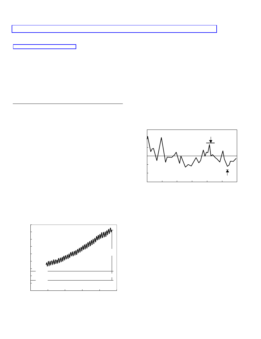
during the past century, as shown in figure 1 (1). The annual cycles in

figure 1 are the result of seasonal variations in plant use of carbon
dioxide. Solid horizontal lines show the levels that prevailed in 1900
and 1940 (2). The magnitude of this atmospheric increase during the
1980s was about 3 gigatons of carbon (Gt C) per year (3). Total hu-
man CO

2

emissions – primarily from use of coal, oil, and natural gas

and the production of cement – are currently about 5.5 GT C per year.

To put these figures in perspective, it is estimated that the atmos-

phere contains 750 Gt C; the surface ocean contains 1,000 Gt C;
vegetation, soils, and detritus contain 2,200 Gt C; and the intermedi-
ate and deep oceans contain 38,000 Gt C (3). Each year, the surface
ocean and atmosphere exchange an estimated 90 Gt C; vegetation
and the atmosphere, 60 Gt C; marine biota and the surface ocean, 50
Gt C; and the surface ocean and the intermediate and deep oceans,
100 Gt C (3).

So great are the magnitudes of these reservoirs, the rates of ex-

change between them, and the uncertainties with which these num-
bers are estimated that the source of the recent rise in atmospheric
carbon dioxide has not been determined with certainty (4). Atmos-
pheric concentrations of CO

2

are reported to have varied widely over

geological time, with peaks, according to some estimates, some 20-
fold higher than at present and lows at approximately 18th-Century
levels (5).

The current increase in carbon dioxide follows a 300-year warm-

ing trend: Surface and atmospheric temperatures have been recover-
ing from an unusually cold period known as the Little Ice Age. The
observed increases are of a magnitude that can, for example, be ex-
plained by oceans giving off gases naturally as temperatures rise. In-
deed, recent carbon dioxide rises have shown a tendency to follow
rather than lead global temperature increases (6).

There is, however, a widely believed hypothesis that the 3 Gt C

per year rise in atmospheric carbon dioxide is the result of the 5.5 Gt C
per year release of carbon dioxide from human activities. This hy-
pothesis is reasonable, since the magnitudes of human release and at-
mospheric rise are comparable, and the atmospheric rise has occurred
contemporaneously with the increase in production of CO

2

from hu-

man activities since the Industrial Revolution.

Environmental Effects of Increased Atmospheric Carbon Dioxide

A

RTHUR

B

.

R

OBINSON ‡ ,

S

ALLIE

L. B

ALIUNAS †

, W

ILLIE

S

OON †

,

AND

Z

ACHARY

W

.

R

OBINSON ‡

‡Oregon Institute of Science and Medicine, 2251 Dick George Rd., Cave Junction, Oregon 97523 [info

@

oism.org]

†George C. Marshall Institute, 1730 K St., NW, Ste 905, Washington, DC 20006 [info

@

marshall.org]

280

290

300

310

320

330

340

350

360

370

1950

1960

1970

1980

1990

2000

Year

CO

2

C

onc

e

nt

ra

ti

on p

pm

1940

1900

82%

18%

20

21

22

23

24

25

26

-1000

-500

0

500

1000

1500

2000

Year

S

ea

S

ur

fac

e

tem

p

er

at

u

re °

C

Medieval Climate Optimum

Little Ice Age

Fig. 1. Atmospheric CO

2

concentrations in parts per million by volume,

ppm, at Mauna Loa, Hawaii. These measurements agree well with those at
other locations (1). Periodic cycle is caused by seasonal variations in CO

2

absorption by plants. Approximate global level of atmospheric CO

2

in 1900 and

1940 is also displayed (2).

Fig. 2. Surface temperatures in the Sargasso Sea (with time resolution of

about 50 years) ending in 1975 as determined by isotope ratios of marine or-
ganism remains in sediment at the bottom of the sea (7). The horizontal line is
the average temperature for this 3,000 year period. The Little Ice Age and
Medieval Climate Optimum were naturally occurring, extended intervals of
climate departures from the mean.

– 1 –

January 1998

ATMOSPHERIC AND SURFACE TEMPERATURES

In any case, what effect is the rise in CO

2

having upon the global

environment? The temperature of the Earth varies naturally over a
wide range. Figure 2 summarizes, for example, surface temperatures
in the Sargaso Sea (a region of the Atlantic Ocean) during the past
3,000 years (7). Sea surface temperatures at this location have varied
over a range of about 3.6 degrees Celsius (ºC) during the past 3,000
years. Trends in these data correspond to similar features that are
known from the historical record.

For example, about 300 years ago, the Earth was experiencing the

‘‘Little Ice Age.’’ It had descended into this relatively cool period
from a warm interval about 1,000 years ago known as the ‘‘Medieval
Climate Optimum.’’ During the Medieval Climate Optimum, tem-
peratures were warm enough to allow the colonization of Greenland.
These colonies were abandoned after the onset of colder temperatures.
For the past 300 years, global temperatures have been gradually recov-
ering (11). As shown in figure 2, they are still a little below the average
for the past 3,000 years. The human historical record does not report
‘‘global warming’’ catastrophes, even though temperatures have been
far higher during much of the last three millennia.

What causes such variations in Earth’s temperature? The answer

may be fluctuations in solar activity. Figure 3 shows the period of

warming from the Little Ice Age in greater detail by means of an 11-
year moving average of surface temperatures in the Northern Hemi-
sphere (10). Also shown are solar magnetic cycle lengths for the
same period. It is clear that even relatively short, half-century-long
fluctuations in temperature correlate well with variations in solar ac-
tivity. When the cycles are short, the sun is more active, hence
brighter; and the Earth is warmer. These variations in the activity of
the sun are typical of stars close in mass and age to the sun (13).

Figure 4 shows the annual average temperatures of the United

States as compiled by the National Climate Data Center (12). The
most recent upward temperature fluctuation from the Little Ice Age
(between 1900 and 1940), as shown in the Northern Hemisphere re-
cord of figure 3, is also evident in this record of U.S. temperatures.
These temperatures are now near average for the past 103 years, with
1996 and 1997 having been the 42nd and 60th coolest years.

Especially important in considering the effect of changes in at-

mospheric composition upon Earth temperatures are temperatures in
the lower troposphere – at an altitude of roughly 4 km. In the tropo-
sphere, greenhouse-gas-induced temperature changes are expected to
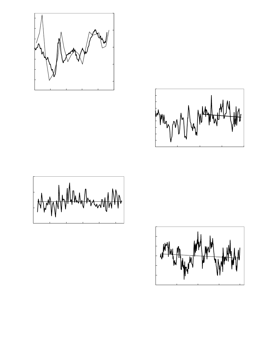
be at least as large as at the surface (14). Figure 5 shows global tropo-
spheric temperatures measured by weather balloons between 1958
and 1996. They are currently near their 40-year mean (15), and have
been trending slightly downward since 1979.

-1.0

-0.8

-0.6

-0.4

-0.2

0.0

0.2

0.4

1750

1800

1850

1900

1950

2000

Year

S

o

la

r

M

agnet

ic C

y

c

le Lengt

h

y

ear

s

18

20

22

24

26

D

e

v

iat

ion f

rom

1951-

1970 M

ean °C

Fig. 3. Moving 11-year average of terrestrial Northern Hemisphere tem-

peratures as deviations in ºC from the 1951-1970 mean – left axis and darker
line (8,9). Solar magnetic cycle lengths – right axis and lighter line (10). The
shorter the magnetic cycle length, the more active, and hence brighter, the sun.

10

11

12

13

1890

1910

1930

1950

1970

1990

Year

U

S

N

a

ti

o

nal T

e

mper

a

tur

e °

C

Fig. 4. Annual mean surface temperatures in the contiguous United States

between 1895 and 1997, as compiled by the National Climate Data Center
(12). Horizontal line is the 103-year mean. The trend line for this 103-year
period has a slope of 0.022 ºC per decade or 0.22 ºC per century. The trend
line for 1940 to 1997 has a slope of 0.008 ºC per decade or 0.08 ºC per century.

-1

-0.8

-0.6

-0.4

-0.2

0

0.2

0.4

0.6

0.8

1958

1968

1978

1988

1998

Year

D

e

viat

io

n f

rom 1979-

1

996 mean °C

Fig. 5. Radiosonde balloon station measurements of global lower tropo-

spheric temperatures at 63 stations between latitudes 90 N and 90 S from 1958
to 1996 (15). Temperatures are three-month averages and are graphed as de-
viations from the mean temperature for 1979 to 1996. Linear trend line for
1979 to 1996 is shown. The slope is minus 0.060 ºC per decade.

-0.6

-0.4

-0.2

0

0.2

0.4

0.6

1978

1983

1988

1993

1998

Year

D

e

v

a

ti

o

n

f

rom

1979-

1996

m

e

an °C

Fig. 6. Satellite Microwave Sounding Unit, MSU, measurements of global

lower tropospheric temperatures between latitudes 83 N and 83 S from 1979 to
1997 (17,18). Temperatures are monthly averages and are graphed as devia-
tions from the mean temperature for 1979 to 1996. Linear trend line for 1979 to
1997 is shown. The slope of this line is minus 0.047 ºC per decade. This record
of measurements began in 1979.

– 2 –

Since 1979, lower-tropospheric temperature measurements have

also been made by means of microwave sounding units (MSUs) on
orbiting satellites (16). Figure 6 shows the average global tropo-
spheric satellite measurements (17,18) – the most reliable measure-
ments, and the most relevant to the question of climate change.

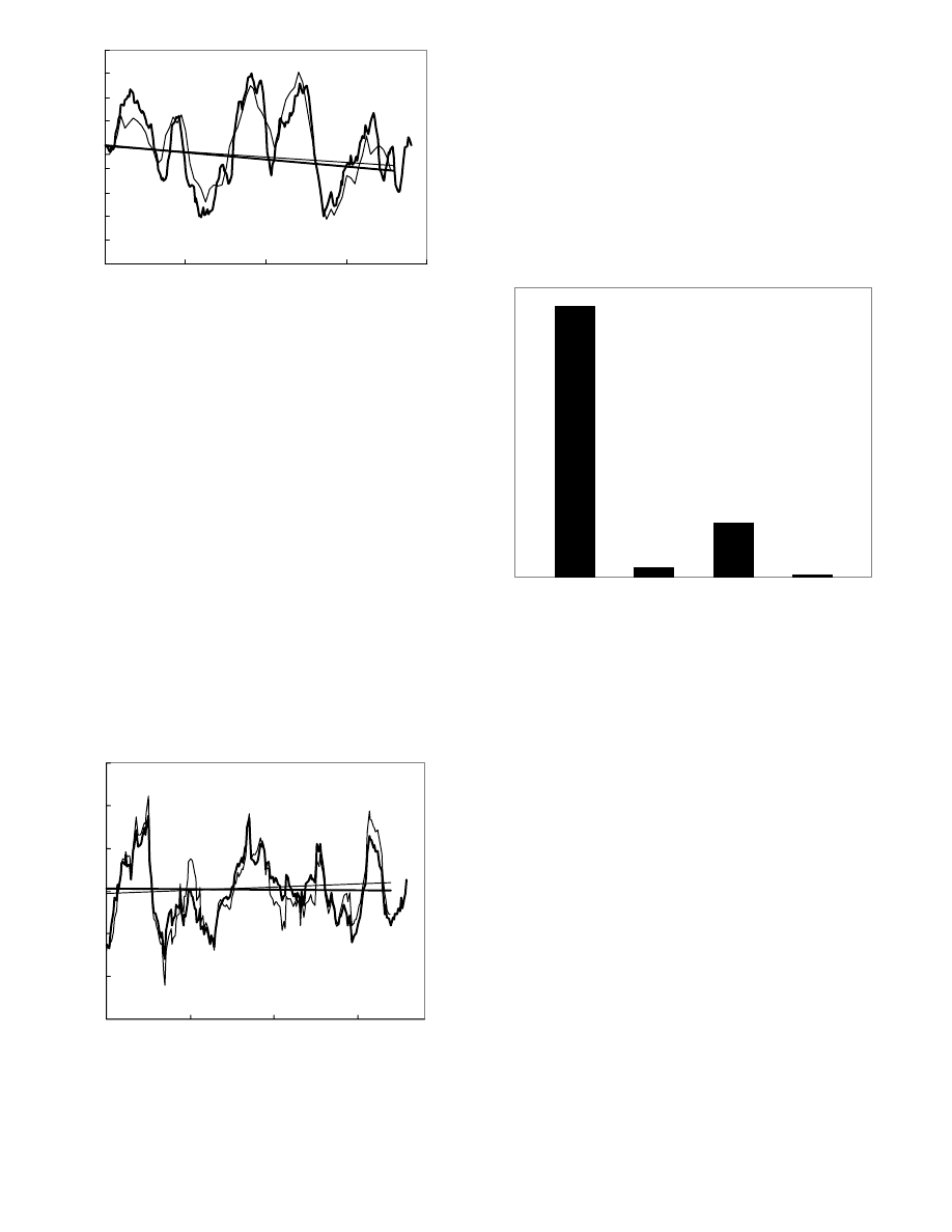
Figure 7 shows the satellite data from figure 6 superimposed upon

the weather balloon data from figure 5. The agreement of the two sets
of data, collected with completely independent methods of measure-
ment, verifies their precision. This agreement has been shown rigor-
ously by extensive analysis (19, 20).

While tropospheric temperatures have trended downward during

the past 19 years by about 0.05 ºC per decade, it has been reported
that global surface temperatures trended upward by about 0.1 ºC per
decade (21, 22). In contrast to tropospheric temperatures, however,
surface temperatures are subject to large uncertainties for several rea-
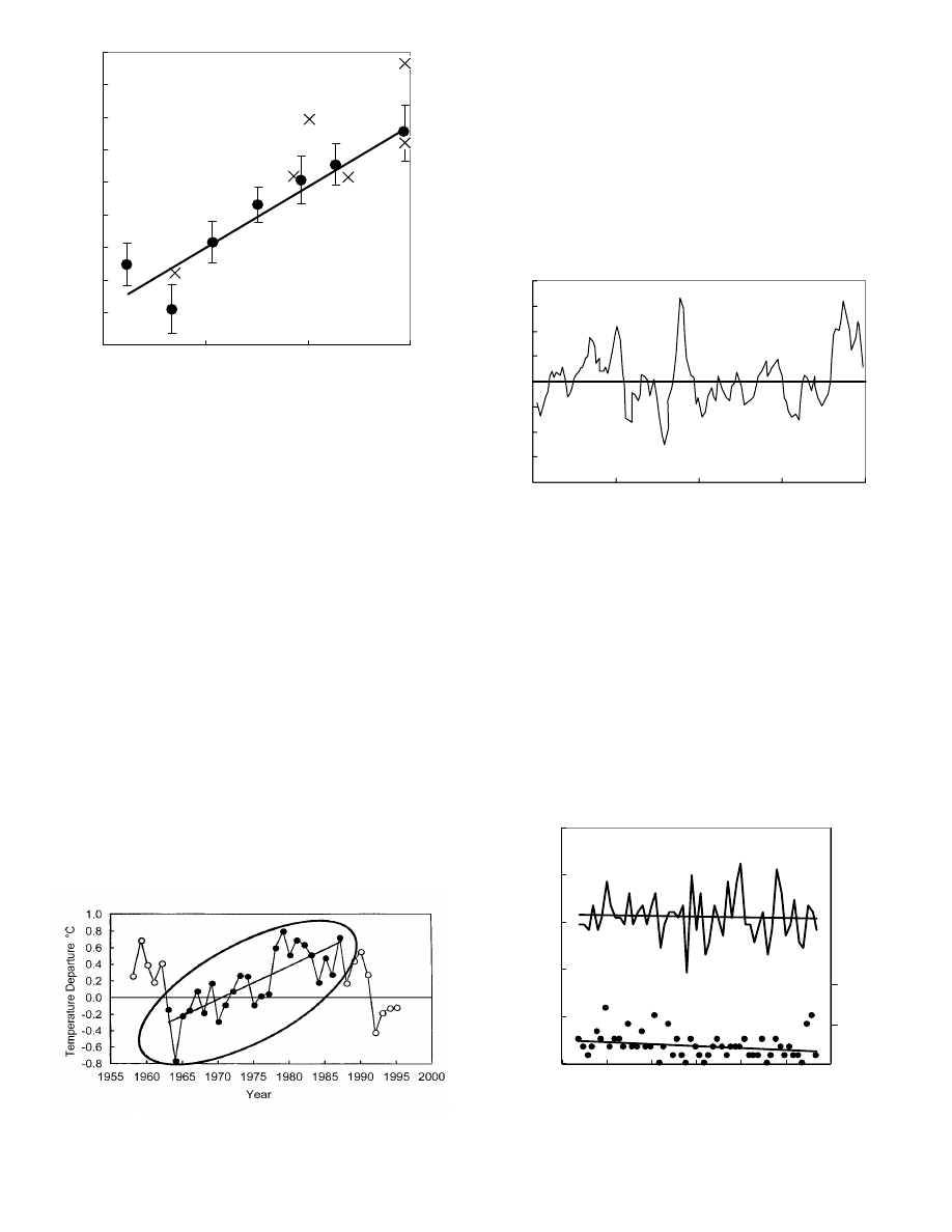
sons, including the urban heat island effect (illustrated below).

During the past 10 years, U.S. surface temperatures have trended

downward by minus 0.08 ºC per decade (12) while global surface tem-
peratures are reported increased by plus 0.03 ºC per decade (23). The
corresponding weather-balloon and satellite tropospheric 10-year
trends are minus 0.4 ºC and minus 0.3 ºC per decade, respectively.

Disregarding uncertainties in surface measurements and giving

equal weight to reported atmospheric and surface data and to 10 and
19 year averages, the mean global trend is minus 0.07 ºC per decade.

In North America, the atmospheric and surface records partly agree

(20 and figure 8). Even there, however, the atmospheric trend is minus
0.01 per decade, while the surface trend is plus 0.07 ºC per decade. The
satellite record, with uniform and better sampling, is much more reliable.

The computer models on which forecasts of global warming are

based predict that tropospheric temperatures will rise at least as much as
surface temperatures (14). Because of this, and because these tempera-
tures can be accurately measured without confusion by complicated ef-
fects in the surface record, these are the temperatures of greatest interest.
The global trend shown in figures 5, 6 and 7 provides a definitive means
of testing the validity of the global warming hypothesis.

THE GLOBAL WARMING HYPOTHESIS

There is such a thing as the greenhouse effect. Greenhouse gases

such as H

2

O and CO

2

in the Earth’s atmosphere decrease the escape

of terrestrial thermal infrared radiation. Increasing CO

2

, therefore, ef-

fectively increases radiative energy input to the Earth. But what hap-
pens to this radiative input is complex: It is redistributed, both
vertically and horizontally, by various physical processes, including
advection, convection, and diffusion in the atmosphere and ocean.

When an increase in CO

2

increases the radiative input to the at-

mosphere, how and in which direction does the atmosphere respond?
Hypotheses about this response differ and are schematically shown in
figure 9. Without the greenhouse effect, the Earth would be about
14 ºC cooler (25). The radiative contribution of doubling atmospheric
CO

2

is minor, but this radiative greenhouse effect is treated quite dif-

ferently by different climate hypotheses. The hypotheses that the IPCC
has chosen to adopt predict that the effect of CO

2

is amplified by the

atmosphere (especially water vapor) to produce a large temperature in-
crease (14). Other hypotheses, shown as hypothesis 2, predict the op-
posite – that the atmospheric response will counteract the CO

2

increase and result in insignificant changes in global temperature (25-
27). The empirical evidence of figures 5-7 favors hypothesis 2. While
CO

2

has increased substantially, the large temperature increase pre-

dicted by the IPCC models has not occurred (see figure 11).

The hypothesis of a large atmospheric temperature increase from

greenhouse gases (GHGs), and further hypotheses that temperature
increases will lead to flooding, increases in storm activity, and cata-
strophic world-wide climatological changes have come to be known

-0.5

-0.4

-0.3

-0.2

-0.1

0

0.1

0.2

0.3

0.4

1979

1984

1989

1994

1999

Year

D

e

v

iat

ion f

rom 1979 -

1996 °C

Fig. 7. Global radiosonde balloon temperature (light line) (15) and global

satellite MSU temperature (dark line) (17,18) from figures 5 and 6 plotted
with 6-month smoothing. Both sets of data are graphed as deviations from
their respective means for 1979 to 1996. The 1979 to 1996 slopes of the trend
lines are minus 0.060 ºC per decade for balloon and minus 0.045 for satellite.

Q

ualit

at

iv

e G

reenhou

s

e

E

ff

e

ct

Present

GHE

Radiative

Effect of CO

2

Hypothesis 1

IPCC

Hypothesis 2

Fig. 9. Qualitative illustration of greenhouse warming. Present: the current

greenhouse effect from all atmospheric phenomena. Radiative effect of CO

2

:

added greenhouse radiative effect from doubling CO

2

without consideration

of other atmospheric components. Hypothesis 1 IPCC: hypothetical amplifi-
cation effect assumed by IPCC. Hypothesis 2: hypothetical moderation effect.

-1.5

-1

-0.5

0

0.5

1

1.5

1979

1984

1989

1994

Years

D

e

v

iat

io

n

f

rom

197

9 -

1

996

°C

Figure 8. Tropospheric temperature measurements by satellite MSU for

North America between 30º to 70º N and 75º to 125º W (dark line) (17, 18)
compared with the surface record for this same region (light line) (24), both
plotted with 12-month smoothing and graphed as deviations from their means
for 1979 to 1996. The slope of the satellite MSU trend line is minus 0.01 ºC
per decade, while that for the surface trend line is plus 0.07 ºC per decade. The
correlation coefficient for the unsmoothed monthly data in the two sets is 0.92.

– 3 –

as ‘‘global warming’’ – a phenomenon claimed to be so dangerous
that it makes necessary a dramatic reduction in world energy use and
a severe program of international rationing of technology (29).

The computer climate models upon which ‘‘global warming’’ is

based have substantial uncertainties. This is not surprising, since the
climate is a coupled, non-linear dynamical system – in layman’s
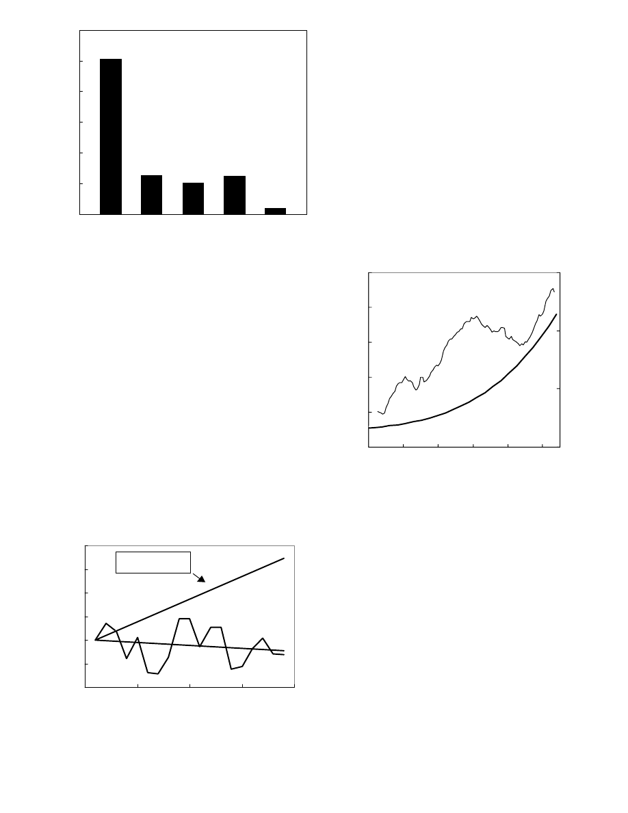
terms, a very complex one. Figure 10 summarizes some of the diffi-
culties by comparing the radiative CO

2

greenhouse effect with cor-

rection factors and uncertainties in some of the parameters in the
computer climate calculations. Other factors, too, such as the effects
of volcanoes, cannot now be reliably computer modeled.

Figure 11 compares the trend in atmospheric temperatures pre-

dicted by computer models adopted by the IPCC with that actually
observed during the past 19 years – those years in which the highest
atmospheric concentrations of CO

2

and other GHGs have occurred.

In effect, an experiment has been performed on the Earth during

the past half-century – an experiment that includes all of the complex
factors and feedback effects that determine the Earth’s temperature
and climate. Since 1940, atmospheric GHGs have risen substantially.
Yet atmospheric temperatures have not risen. In fact, during the 19
years with the highest atmospheric levels of CO

2

and other GHGs,

temperatures have fallen.

Not only has the global warming hypothesis failed the experimen-

tal test; it is theoretically flawed as well. It can reasonably be argued
that cooling from negative physical and biological feedbacks to
GHGs will nullify the initial temperature rise (26, 30).

The reasons for this failure of the computer climate models are

subjects of scientific debate. For example, water vapor is the largest
contributor to the overall greenhouse effect (31). It has been sug-
gested that the computer climate models treat feedbacks related to
water vapor incorrectly (27, 32).

The global warming hypothesis is not based upon the radiative

properties of the GHGs themselves. It is based entirely upon a small
initial increase in temperature caused by GHGs and a large theoreti-
cal amplification of that temperature change. Any comparable tem-
perature increase from another cause would produce the same
outcome from the calculations.

At present, science does not have comprehensive quantitative

knowledge about the Earth’s atmosphere. Very few of the relevant
parameters are known with enough rigor to permit reliable theoretical
calculations. Each hypothesis must be judged by empirical results.
The global warming hypothesis has been thoroughly evaluated. It
does not agree with the data and is, therefore, not validated.

GLOBAL WARMING EVIDENCE

Aside from computer calculations, two sorts of evidence have

been advanced in support of the ‘‘global warming’’ hypothesis: tem-
perature compilations and statements about global flooding and
weather disruptions. Figure 12 shows the global temperature graph
that has been compiled by National Aeronautic and Space Admini-
stration’s Goddard Institute of Space Studies (NASA GISS) (23, 33,
and 34). This compilation, which is shown widely in the press, does
not agree with the atmospheric record because surface records have
substantial uncertainties (36). Figure 13 illustrates part of the reason.

The urban heat island effect is only one of several surface effects

that can confound compiled records of surface temperature. Figure
13 shows the size of this effect in, for example, the surface stations of
California and the problems associated with objective sampling. The

-0.4

-0.2

0

0.2

0.4

0.6

0.8

1978

1983

1988

1993

1998

Year

T

e

m

per

at

ur

e c

hange

f

rom

1979 °

C

IPCC Predicted Global

Warming Trend

Fig. 11. Global annual lower tropospheric temperatures as measured by

satellite MSU between latitudes 83 N and 83 S (17, 18) plotted as deviations
from the 1979 value. The trend line of these experimental measurements is
compared with the corresponding trend line predicted by International Panel
on Climate Change (IPCC) computer climate models (14).

0

20

40

60

80

100

120

1

2

3

4

5

6

7

8

9

10

11

W

a

tt

s

pe

r

s

quar

e m

e

te

r

O c ean Surfac e

F lux C o rrec tio n

N o rth-So ut h
H eat F lux B y

M o tio ns

H um idity

C lo uds

G reenho us e

(D o ubled C O 2)

Fig. 10. The radiative greenhouse effect of doubling the concentration of

atmospheric CO

2

(right bar) as compared with four of the uncertainties in the

computer climate models (14, 28).

-0.2

0

0.2

0.4

0.6

0.8

1880

1900

1920

1940

1960

1980

Years

T

e

m

per

at

ur

e C

h

ange °C

280

310

340

370

C

O

2 C

onc

ent

ra

ti

on

Figure 12. Eleven-year moving average of global surface temperature, as

estimated by NASA GISS (23, 33, and 34), plotted as deviation from 1890
(left axis and light line), as compared with atmospheric CO

2

(right axis and

dark line) (2). Approximately 82% of the increase in CO

2

occurred after the

temperature maximum in 1940, as is shown in figure 1.

The new high in temperature estimated by NASA GISS after 1940 is not

present in the radiosonde balloon measurements or the satellite MSU meas-
urements. It is also not present in surface measurements for regions with com-
prehensive, high-quality temperature records (35). The United States surface
temperature record (see figure 4) gives 1996 and 1997 as the 38th and 56th
coolest years in the 20th century. Biases and uncertainties, such as that shown
in figure 13, account for this difference.

– 4 –

East Park station, considered the best situated rural station in the state
(37), has a trend since 1940 of minus 0.055 ºC per decade.

The overall rise of about plus 0.5 ºC during the 20th century is often

cited in support of ‘‘global warming’’ (38). Since, however, 82% of
the CO

2

rise during the 20th century occurred after the rise in tempera-

ture (see figures 1 and 12), the CO

2

increase cannot have caused the

temperature increase. The 19th century rise was only 13 ppm (2).

In addition, incomplete regional temperature records have been

used to support ‘‘global warming.’’ Figure 14 shows an example of
this, in which a partial record was used in an attempt to confirm com-
puter climate model predictions of temperature increases from green-
house gases (41). A more complete record refuted this attempt (42).

Not one of the temperature graphs shown in figures 4 to 7, which

include the most accurate and reliable surface and atmospheric tem-
perature measurements available, both global and regional, shows
any warming whatever that can be attributed to increases in green-
house gases. Moreover, these data show that present day tempera-
tures are not at all unusual compared with natural variability, nor are
they changing in any unusual way.

SEA LEVELS AND STORMS

The computer climate models do not make any reliable predic-

tions whatever concerning global flooding, storm variability, and
other catastrophes that have come to be a part of the popular defini-
tion of ‘‘global warming.’’ (See Chapter 6, section 6-5 of reference
14.) Yet several scenarios of impending global catastrophe have
arisen separately. One of these hypothesizes that rising sea levels will
flood large areas of coastal land. Figure 15 shows satellite measure-
ments of global sea level between 1993 and 1997 (43). The reported
current global rate of rise amounts to only about plus 2 mm per year,
or plus 8 inches per century, and even this estimate is probably high
(43). The trends in rise and fall of sea level in various regions have a

wide range of about 100 mm per year with most of the globe showing
downward trends (43). Historical records show no acceleration in sea
level rise in the 20th century (44). Moreover, claims that global
warming will cause the Antarctic ice cap to melt and sharply increase
this rate are not consistent with experiment or with theory (45).

Similarly, claims that hurricane frequencies and intensities have

been increasing are also inconsistent with the data. Figure 16 shows
the number of severe Atlantic hurricanes per year and also the maxi-
mum wind intensities of those hurricanes. Both of these values have
been decreasing with time.

-0.1

0

0.1

0.2

0.3

0.4

0.5

0.6

0.7

0.8

10,000

100,000

1,000,000

10,000,000

Population of County

T

e

m

per

at

ur

e t

rend per

D

e

c

a

de 1940-

1996

°

C

Fig. 13. Surface temperature trends for the period of 1940 to 1996 from

107 measuring stations in 49 California counties (39, 40). After averaging the
means of the trends in each county, counties of similar population were com-
bined and plotted as closed circles along with the standard errors of their
means. The six measuring stations in Los Angeles County were used to calcu-
late the standard error of that county, which is plotted alone at the county
population of 8.9 million. The ‘‘urban heat island effect’’ on surface measure-
ments is evident. The straight line is a least-squares fit to the closed circles.
The points marked ‘‘X’’ are the six unadjusted station records selected by
NASA GISS (23, 33, and 34) for use in their estimate of global temperatures
as shown in figure 12.

Fig. 14 The solid circles in the oval are tropospheric temperatures for the

Southern Hemisphere between latitudes 30 S and 60 S, published in 1996 (41)
in support of computer-model-projected warming. Later in 1996, the study
was refuted by a longer set of data, as shown by the open circles (42).

-8

-6

-4

-2

0

2

4

6

8

1993

1994

1995

1996

1997

Year

S

e

a

Lev

el

c

h

ange

m

il

lim

et

e

rs

Fig. 15. Global sea level measurements from the Topex/Poseidon satellite

altimeter for 1993 to 1997 (43). The instrument record gives a rate of change of
minus 0.2 mm per year (43). However, it has been reported that 50-year tide
gauge measurements give plus 1.8 mm per year. A correction of plus 2.3 mm
per year was added to the satellite data based on comparison to selected tide
gauges to get a value of plus 2.1 mm per year or 8 inches per century (43).

.

0

20

40

60

80

100

1940

1950

1960

1970

1980

1990

2000

Year

M

a

x

im

u

m

at

ta

in

ed

W

ind S

p

eed

M

e

te

rs

per

S

e

c

ond

Num

ber

of

V

iol

en

t H

u

rr

ic

anes

0

5

10

Fig. 16. Annual numbers of violent hurricanes and maximum attained

wind speeds during those hurricanes in the Atlantic Ocean (46). Slopes of the
trend lines are minus 0.25 hurricanes per decade and minus 0.33 meters per
second maximum attained wind speed per decade.

– 5 –

As temperatures recover from the Little Ice Age, the more extreme

weather patterns that characterized that period may be trending
slowly toward the milder conditions that prevailed during the Middle
Ages, which enjoyed average temperatures about 1 ºC higher than
those of today. Concomitant changes are also taking place, such as
the receding of glaciers in Montana’s Glacier National Park.

FERTILIZATION OF PLANTS

How high will the carbon dioxide concentration of the atmosphere

ultimately rise if mankind continues to use coal, oil, and natural gas?
Since total current estimates of hydrocarbon reserves are approxi-
mately 2,000 times annual use (47), doubled human release could,
over a thousand years, ultimately be 10,000 GT C or 25% of the
amount now sequestered in the oceans. If 90% of this 10,000 GT C
were absorbed by oceans and other reservoirs, atmospheric levels
would approximately double, rising to about 600 parts per million.
(This assumes that new technologies will not supplant the use of hy-
drocarbons during the next 1,000 years, a pessimistic estimate of
technological advance.)

One reservoir that would moderate the increase is especially im-

portant. Plant life provides a large sink for CO

2

. Using current

knowledge about the increased growth rates of plants and assuming a
doubling of CO

2

release as compared to current emissions, it has

been estimated that atmospheric CO

2

levels will rise by only about

300 ppm before leveling off (2). At that level, CO

2

absorption by in-

creased Earth biomass is able to absorb about 10 GT C per year.

As atmospheric CO

2

increases, plant growth rates increase. Also,

leaves lose less water as CO

2

increases, so that plants are able to grow

under drier conditions. Animal life, which depends upon plant life for
food, increases proportionally.

Figures 17 to 22 show examples of experimentally measured in-

creases in the growth of plants. These examples are representative of
a very large research literature on this subject (49-55). Since plant re-
sponse to CO

2

fertilization is nearly linear with respect to CO

2

con-

centration over a range of a few hundred ppm, as seen for example in
figures 18 and 22, it is easy to normalize experimental measurements
at different levels of CO

2

enrichment. This has been done in figure 23

in order to illustrate some CO

2

growth enhancements calculated for

the atmospheric increase of about 80 ppm that has already taken
place, and that expected from a projected total increase of 320 ppm.

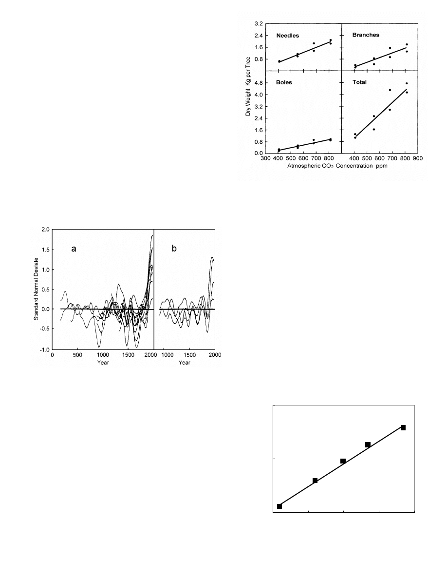
As figure 17 shows, long-lived (1,000- to 2000-year-old) pine

trees have shown a sharp increase in growth rate during the past half-
century. Figure 18 summarizes the increased growth rates of young
pine seedlings at four CO

2

levels. Again, the response is remarkable,

with an increase of 300 ppm more than tripling the rate of growth.

Figure 19 shows the 30% increase in the forests of the United

States that has taken place since 1950. Much of this increase is likely
due to the increase in atmospheric CO

2

that has already occurred. In

addition, it has been reported that Amazonian rain forests are increas-
ing their vegetation by about 34,000 moles (900 pounds) of carbon
per acre per year (57), or about two tons of biomass per acre per year.

Figure 20 shows the effect of CO

2

fertilization on sour orange

trees. During the early years of growth, the bark, limbs, and fine roots
of sour orange trees growing in an atmosphere with 700 ppm of CO

2

exhibited rates of growth more than 170% greater than those at 400
ppm. As the trees matured, this slowed to about 100%. Meanwhile,
orange production was 127% higher for the 700 ppm trees.

Trees respond to CO

2

fertilization more strongly than do most

other plants, but all plants respond to some extent. Figure 21 shows
the response of wheat grown under wet conditions and when the
wheat was stressed by lack of water. These were open-field experi-
ments. Wheat was grown in the usual way, but the atmospheric CO

2

concentrations of circular sections of the fields were increased by
means of arrays of computer-controlled equipment that released CO

2

into the air to hold the levels as specified.

While the results illustrated in figures 17-21 are remarkable, they

are typical of those reported in a very large number of studies of the
effect of CO

2

concentration upon the growth rates of plants (49-55).

Figure 22 summarizes 279 similar experiments in which plants of

Fig. 17. Standard normal deviates of tree ring widths for (a) bristlecone

pine, limber pine, and fox tail pine in the Great Basin of California, Nevada,
and Arizona and (b) bristlecone pine in Colorado (48). The tree ring widths
have been normalized so that their means are zero and deviations from the
means are displayed in units of standard deviation.

600

700

800

1950

1960

1970

1980

1990

Year

H

a

rd

w

o

ods

and S

o

ft

w

oods

B

illio

n

s

o

f Cu

b

ic

F

e

e

t

Fig. 18. Young Eldarica pine trees were grown for 23 months under four

CO

2

concentrations and then cut down and weighed. Each point represents an

individual tree (56). Weights of tree parts are as indicated.

Fig. 19. Inventories of standing hardwood and softwood timber in the

United States compiled from Forest Statistics of the United States (58).

– 6 –

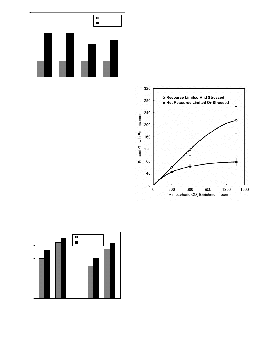
various types were raised under CO

2

-enhanced conditions. Plants un-

der stress from less-than-ideal conditions – a common occurrence in
nature – respond more to CO

2

fertilization. The selections of species

shown in figure 22 were biased toward plants that respond less to
CO

2

fertilization than does the mixture actually covering the Earth,

so figure 22 underestimates the effects of global CO

2

enhancement.

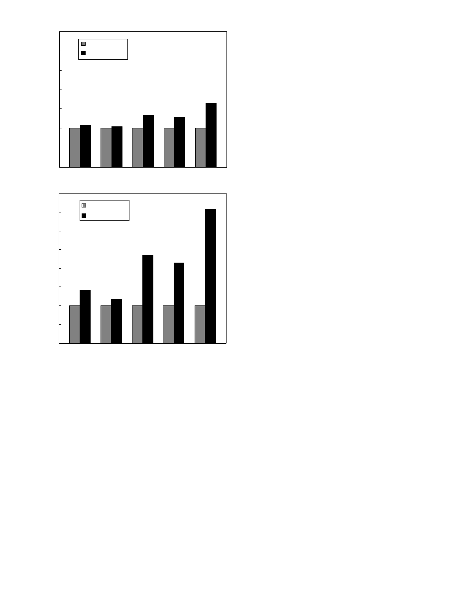
Figure 23 summarizes the wheat, orange tree, and young pine tree

enhancements shown in figures 21, 20, and 18 with two atmospheric
CO

2

increases – that which has occurred since 1800 and is believed

to be the result of the Industrial Revolution and that which is pro-
jected for the next two centuries. The relative growth enhancement of
trees by CO

2

diminishes with age. Figure 23 shows young trees.

Clearly, the green revolution in agriculture has already benefited

from CO

2

fertilization; and benefits in the future will likely be spec-

tacular. Animal life will increase proportionally as shown by studies
of 51 terrestrial (63) and 22 aquatic ecosystems (64). Moreover, as
shown by a study of 94 terrestrial ecosystems on all continents except
Antarctica (65), species richness (biodiversity) is more positively cor-
related with productivity – the total quantity of plant life per acre –
than with anything else.

DISCUSSION

There are no experimental data to support the hypothesis that in-

creases in carbon dioxide and other greenhouse gases are causing or
can be expected to cause catastrophic changes in global temperatures
or weather. To the contrary, during the 20 years with the highest carb-
on dioxide levels, atmospheric temperatures have decreased.

We also need not worry about environmental calamities, even if

the current long-term natural warming trend continues. The Earth has
been much warmer during the past 3,000 years without catastrophic
effects. Warmer weather extends growing seasons and generally im-
proves the habitability of colder regions. ‘‘Global warming,’’ an in-
validated hypothesis, provides no reason to limit human production
of CO

2

, CH

4

, N

2

O, HFCs, PFCs, and SF

6

as has been proposed (29).

Human use of coal, oil, and natural gas has not measurably

warmed the atmosphere, and the extrapolation of current trends
shows that it will not significantly do so in the foreseeable future. It
does, however, release CO

2,

which accelerates the growth rates of

plants and also permits plants to grow in drier regions. Animal life,
which depends upon plants, also flourishes.

As coal, oil, and natural gas are used to feed and lift from poverty

vast numbers of people across the globe, more CO

2

will be released

into the atmosphere. This will help to maintain and improve the
health, longevity, prosperity, and productivity of all people.

Human activities are believed to be responsible for the rise in CO

2

level of the atmosphere. Mankind is moving the carbon in coal, oil,
and natural gas from below ground to the atmosphere and surface,
where it is available for conversion into living things. We are living
in an increasingly lush environment of plants and animals as a result
of the CO

2

increase. Our children will enjoy an Earth with far more

plant and animal life as that with which we now are blessed. This is a
wonderful and unexpected gift from the Industrial Revolution.

0

100

200

300

400

R

elat

iv

e G

ro

w

th

400 ppm CO2

700 ppm CO2

171

%

175

%

107

%

127

%

Trunk & Limbs

Y oung

Orange Trees

Fine Roots

Y oung

Orange Trees

Trunk & Limbs

Mature

Orange Trees

Oranges

per Tree

0

2000

4000

6000

8000

10000

1

G

rai

n Y

iel

d K

g

pe

r hec

ta

re

370 ppm CO2

550 ppm CO2

Dry

Dry

Wet

Wet

1992-93

1993-94

12%

21%

25%

8%

Fig. 20. Relative trunk and limb volumes and fine root biomass of young

sour orange trees; and trunk and limb volumes and numbers of oranges pro-
duced per mature sour orange tree per year at 400 ppm CO

2

(light bars) and

700 ppm CO

2

(dark bars) (59, 60). The 400 ppm values were normalized to

100. The trees were planted in 1987 as one-year-old seedlings. Young trunk
and limb volumes and fine root biomass were measured in 1990. Mature trunk
and limb volumes are averages for 1991 to 1996. Orange numbers are aver-
ages for 1993 to 1997.

Fig. 21. Grain yields from wheat grown under well watered and poorly

watered conditions in open field experiments (61, 62). Average CO

2

-induced

increases for the two years were 10% for wet and 23% for dry conditions.

Fig. 22. Summary data from 279 published experiments in which plants

of all types were grown under paired stressed (open circles) and unstressed
(closed circles) conditions (66). There were 208, 50, and 21 sets at 300, 600,
and an average of about 1350 ppm CO

2

, respectively. The plant mixture in the

279 studies was slightly biased toward plant types that respond less to CO

2

fertilization than does the actual global mixture and therefore underestimates
the expected global response. CO

2

enrichment also allows plants to grow in

drier regions, further increasing the expected global response.

– 7 –

REFERENCES

0

50

100

150

200

250

300

350

1

2

3

4

5

6

7

8

9 10 11 12 13 14 15 16

P

ro

d

u

c

ti

o

n

N

o

rm

a

lize

d

t

o

10

0 at

28

0 pp

m

280 ppm CO2

360 ppm CO2

Dry Wheat Wet Wheat Oranges

Orange

Trees

Young

Pine Trees

10%

4%

34%

29%

65%

0

50

100

150

200

250

300

350

400

1

2

3

4

5

6

7

8

9 10 11 12 13 14 15 16

P

ro

d

u

c

ti

on

N

o

rm

alized

t

o

10

0 a

t 28

0 p

p

m

280 ppm CO2

600 ppm CO2

Dry Wheat Wet Wheat Oranges

Orange

Trees

Young

Pine Trees

18%

41%

135%

265%

114%

Fig. 23. Calculated growth rate enhancement of wheat, young orange

trees, and very young pine trees already taking place as a result of atmospheric
enrichment by CO

2

during the past two centuries (a) and expected to take

place as a result of atmospheric enrichment by CO

2

to a level of 600 ppm (b).

In this case, these values apply to pine trees during their first two years of

growth and orange trees during their 4th through 10th years of growth. As is
shown in figure 20, the effect of increased CO

2

gradually diminishes with tree

age, so these values should not be interpreted as applicable over the entire tree
lifespans. There are no longer-running controlled CO

2

tree experiments. Yet,

even 2,000 year old trees still respond significantly as is shown in figure 17.

a

b

– 8 –

1.

2.

3.
4.

5.
6.
7.
8.
9.
10.

Keeling, C. D. and Whorf, T. P. (1997) Trends Online: A Compendium of Data
on Global Change, Carbon Dioxide Information Analysis Center, Oak Ridge
National Laboratory; [http://cdiac.esd.ornl.gov/ftp/ndp001r7/].
Idso, S. B. (1989) Carbon Dioxide and Global Change: Earth in Transition, IBR
Press, 7.
Schimel, D. S. (1995) Global Change Biology 1, 77-91.
Segalstad, T. V. (1998) Global Warming the Continuing Debate, Cambridge
UK: Europ. Sci. and Environ. For., ed. R. Bate, 184-218.
Berner, R. A. (1997) Science 276, 544-545.
Kuo, C., Lindberg, C. R., and Thornson, D. J. (1990) Nature 343,709-714.
Kegwin, L. D. (1996) Science 274, 1504-1508; [[e-mail]].
Jones, P. D. et. al. (1986) J. Clim. Appl. Meterol. 25, 161-179.
Grovesman, B. S. and Landsberg, H. E. (1979) Geophys. Res. Let. 6, 767-769.
Baliunas, S. and Soon, W. (1995) Astrophysical Journal 450, 896-901; Friis-
Christensen, E. and Lassen, K. (1991) Science 254, 698-700; [sbaliunas,
[e-mail]].

11.

12.

13.
14.

15.

16.

17.
18.

19.
20.
21.
22.
23.

24.

25.
26.
27.

28.

29.

30.

31.

32.

33.
34.
35.

36.
37.
38.
39.

40.
41.
42.

43.

44.
45.

46.

47.
48.
49.
50.
51.
52.
53.
54.
55.
56.
57.
58.

59.
60.
61.
62.

63.

64.
65.
66.

Lamb, H. H. (1982) Climate, History, and the Modern World, pub New York:
Methuen.
Brown, W. O. and Heim, R. R. (1996) National Climate Data Center, Climate
Variation Bulletin 8, Historical Climatology Series 4-7, Dec.; [http://www.
ncdc.noaa. gov/o1/documentlibrary/cvb.html/].
Baliunas, S. L. et. al. (1995) Astrophysical Journal 438, 269-287.
Houghton, J. T. et. al. (1995) Report of the Intergovernmental Panel on Climate
Change, Cambridge University Press.
Angell, J. K. (1997) Trends Online: A Compendium of Data on Global Change,
Oak Ridge National Laboratory; [http://cdiac.esd.ornl.gov/ftp/ndp008r4/].
Spencer, R. W., Christy, J. R., and Grody, N. C. (1990) Journal of Climate 3,
1111-1128.
Spencer, R. W. and Christy, J. R. (1990) Science 247, 1558-1562.
Christy, J. R., Spencer, R. W., and Braswell, W. D. (1997) Nature 389, 342;
Christy, J. R. personal comm; [http://wwwghrc.msfc.nasa.gov/ims-cgi-bin/mkda
ta?msu2rm190+/pub/data/msu/limb90/chan2r/].
Spencer, R. W. and Christy, J. R. (1992) Journal of Climate 5, 847-866.
Christy, J. R. (1995) Climatic Change 31, 455-474.
Jones, P. D. (1994) Geophys. Res. Let. 21, 1149-1152.
Parker, D. E., et. al. (1997) Geophys. Res. Let. 24, 1499-1502.
Hansen, J., Ruedy, R. and Sato, M. (1996) Geophys. Res. Let. 23, 1665-1668;
[http://www.giss.nasa.gov/data/gistemp/].
The Climate Research Unit, East Anglia University, United Kingdom;
[http://www.cru.uea.ac.uk/advance10k/climdata.htm/].
Lindzen, R. S. (1994) Ann. Review Fluid. Mech. 26, 353-379.
Sun, D. Z. and Lindzen, R. S. (1993) Ann. Geophysicae 11, 204-215.
Spencer, R. W. and Braswell, W. D. (1997) Bull. Amer. Meteorolog. Soc. 78,
1097-1106.
Baliunas, S. (1996) Uncertainties in Climate Modeling: Solar Variability and
Other Factors, Committee on Energy and Natural Resources; United States Sen-
ate. Lindzen, R. S. (1995), personal communication.
Kyoto Protocol to the United Nations Framework Convention on Climate
Change (1997). Adoption of this protocol would sharply limit GHG release for
one-fifth of the world’s people and nations, including the United States.
Idso, S. B. (1997) in Global Warming: The Science and the Politics, ed. L. Jones,
The Fraser Institute: Vancouver, 91-112.
Lindzen, R. S. (1996) in Climate Sensitivity of Radiative Perturbations: Physical
Mechanisms and Their Validation, NATO ASI Series I34, ed. H. Le Treut, Ber-
lin-Heidelberg: Springer-Verlag, 51-66.
Renno, N. O., Emanuel, K. A., and Stone, P. H. (1994) J. Geophysical Research
99, 14429-14441.
Hansen, J. and Lebedeff, S. (1987) J. Geophysical Research 92, 13345-13372.
Hansen, J. and Lebedeff, S. (1988) Geophys. Res. Let. 15, 323-326.
Christy, J. R. (1997) The Use of Satellites in Global Warming Forecasts, George
C. Marshall Institute.
Balling, Jr., R. C. The Heated Debate (1992), Pacific Research Institute.
Goodridge, J. D. (1998) private communication.
Schneider, S. H. (1994) Science 263, 341-347.
Goodridge, J. D. (1996) Bulletin of the American Meteorological Society 77, 3-4;
Goodridge, J. D. private communication.
Christy, J. R. and Goodridge, J. D. (1995) Atm. Envir. 29, 1957-1961.
Santer, B. D., et. al. (1996) Nature 382, 39-45.
Michaels, P. J. and Knappenberger, P. C. (1996) Nature 384, 522-523; [pjm8x,pc
[e-mail]]; Weber, G. O. (1996) Nature 384, 523-524; Also, San-
ter, B. D. (1996) Nature 384, 524.
Nerem, R. S. et. al. (1997) Geophys. Res. Let. 24, 1331-1334; [nerem@
csr.utexas.edu]; Douglas, B. C. (1995) Rev. Geophys. Supplement 1425-1432.
Douglas, B. C. (1992) J. Geophysical Research 97, 12699-12706.
Bentley, C. R. (1997) Science 275, 1077-1078; Nicholls, K. W. (1997) Nature
388, 460-462.
Landsea, C. W., et. al. (1996) Geophys. Res. Let. 23, 1697-1700; [landsea
@aoml.noaa.gov].
Penner, S. S. (1998) Energy – The International Journal, January, in press.
Graybill, D. A. and Idso, S. B. (1993) Global. Biogeochem. Cyc. 7, 81-95.
Kimball, B. A. (1983) Agron. J. 75, 779-788.
Poorter, H. (1993) Vegetatio 104-105, 77-97.
Cure, J. D. and Acock, B. (1986) Agric. For. Meteorol. 8, 127-145.
Gifford, R. M. (1992) Adv. Bioclim. 1, 24-58.
Mortensen, L. M. (1987) Sci. Hort. 33, 1-25.
Drake, B. G. and Leadley, P. W. (1991) Plant, Cell, and Envir. 14, 853-860.
Lawlor, D. W. and Mitchell, R. A. C. (1991) Plant, Cell, and Envir. 14, 807-818.
Idso, S. B. and Kimball, B. A. (1994) J. Exper. Botany 45, 1669-1692.
Grace, J., et. al. (1995) Science 270, 778-780.
Waddell, K. L., Oswald, D. D., and Powell D. S. (1987) Forest Statistics of the
United States, U. S. Forest Service and Dept. of Agriculture.
Idso, S. B. and Kimball, B. A., (1997) Global Change Biol. 3, 89-96.
Idso, S. B. and Kimball, B. A. (1991) Agr. Forest Meteor. 55, 345-349.
Kimball, et. al. (1995) Global Change Biology 1, 429-442.
Pinter, J. P. et. al., (1996) Carbon Dioxide and Terrestrial Ecosystems, ed. G. W.
Koch and H. A. Mooney, Academic Press.
McNaughton, S. J., Oesterhold, M., Frank. D. A., and Williams, K. J. (1989) Na-
ture 341, 142-144.
Cyr, H. and Pace, M. L. (1993) Nature 361, 148-150.
Scheiner, S. M. and Rey-Benayas, J. M. (1994) Evol. Ecol. 8, 331-347.
Idso, K. E. and Idso, S. (1974) Agr. and Forest Meteorol. 69, 153-203.