Sensors - February 2002 - Demystifying Analog Filter Design

Page 1 of 12

http://www.sensorsmag.com/articles/0202/filter/main.shtml

10/03/2002

FEBRUARY 2002

Demystifying

Analog Filter Design

Armed with a little help—and a little math—you can hack your way
fearlessly through the wild world of analog filter design and gain the
confidence that comes with doing it yourself.

Simon Bramble, Maxim Integrated Products

I

t’s a jungle out there. A small tribe, hidden from view in the dense

wilderness, is much sought after by headhunters from the
surrounding plains. The tribe knows it’s threatened, because its
numbersækilled off by the accelerating advance of modern
technologyæare dwindling at an alarming rate. This is the tribe of the
Analog Engineers. The guru of Analog Engineers is the Analog Filter
Designer, who sits on the throne of the besieged kingdom and
imparts wisdom while reminiscing of better days.

But you’re desperate. Your boss told you to design a data acquisition
system, and that means you need an analog filter—fast. You try a
book on filter design. Alas! The countless pages of equations found
in such books can frighten small dogs and children, let alone
engineers. What to do?

Fear not! This article unravels the mystery of filter design so that you
can design continuous-time analog filters quickly and with a
minimum of mathematics. The throne will soon be vacant.

The Theory of Analog Electronics

Analog electronics has two distinct sides: theory (e.g., using the
equations of stability and phase-shift calculations), taught by
academic institutions, and practical considerations (e.g., avoiding
oscillation by tweaking the gain with a capacitor), familiar to most
engineers. Unfortunately, filter design is based firmly on long-
established equations and tables of theoretical results. The theoretical
equations can prove arduous, so this article uses a minimum of
mathæeither in translating the theoretical tables into practical
component values or in deriving the response of a general-purpose
filter.

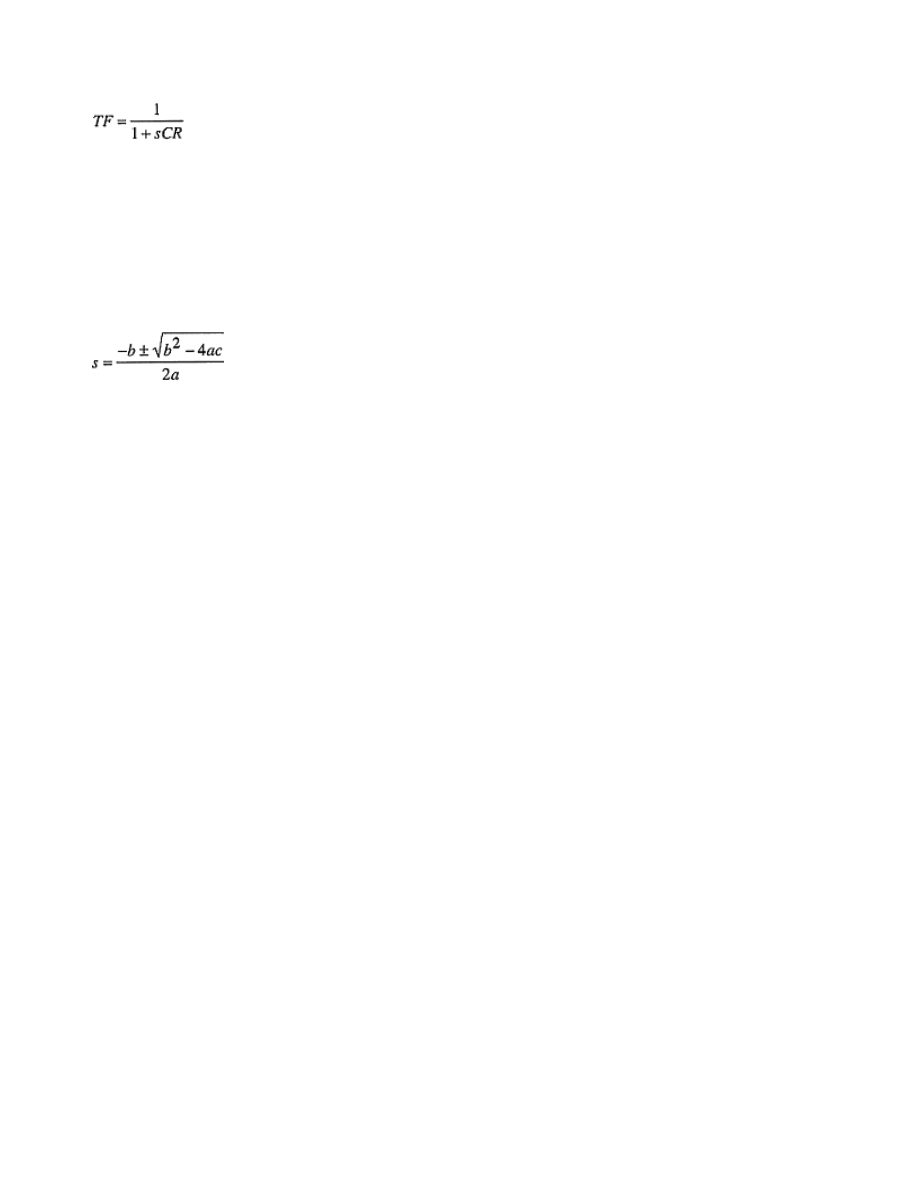
Simple RC low-pass filters have the following transfer function:

SENSOR

TECHNOLOGY AND DESIGN

- Select -

March 10, 2002

Industry News

Updated Twice Weekly

•

Xicor's New Architecture

Addresses Growing Market

•

OmniVision Opens

European Office

•

Building Automation

Systems Buy Into Internet, IT

•

Intelligent Instrumentation,

Entivity Partner

News From Sensors

Order Now!

Sensors - February 2002 - Demystifying Analog Filter Design

Page 2 of 12

http://www.sensorsmag.com/articles/0202/filter/main.shtml

10/03/2002

Cascading such filters complicates the response by giving rise to
quadratic equations in the denominator of the transfer function. Thus,
the denominator of the transfer function for any second-order low-

pass filter is as

2

+ bs + c. Substituting values for a, b, and c

determines the filter response over frequency. Anyone who
remembers high school math will note that the preceding expression
equals zero for certain values of s given by the equation:

At the values of s for which this quadratic equation equals zero, the
transfer function theoretically has infinite gain. These values, which
establish the performance of each type of filter over frequency, are
known as the poles of the quadratic equation. Poles usually occur as
pairs, in the form of a complex number (a + jb) and its complex
conjugate (a – jb). The term jb is sometimes zero.

The thought of a transfer function with infinite gain may frighten
you, but in practice, it isn’t a problem. The pole’s real part, a,
indicates how the filter responds to transients; its imaginary part, jb,
indicates the response over frequency. As long as this imaginary part
is negative (as it must be), the system is stable. The following
discussion explains how to transfer the tables of poles found in many
textbooks into component values suitable for circuit design.

Filter Types

The most common filter responses are the Butterworth, Chebyshev,
and Bessel types. Many other types are available, but 90% of all
applications can be solved with one of these three.

A Butterworth filter ensures a flat response in the pass band and an
adequate rate of rolloff. A good all-round filter, the Butterworth is
simple to understand and suitable for such applications as audio
processing.

A Chebyshev filter gives a much steeper rolloff, but pass-band ripple
makes it unsuitable for audio systems. It’s superior for applications
in which the pass band includes only one frequency of interest (e.g.,
the derivation of a sine wave from a square wave by filtering out the
harmonics).

A Bessel filter gives a constant propagation delay across the input
frequency spectrum. Therefore, applying a square wave (consisting
of a fundamental and many harmonics) to the input of a Bessel filter

(1)

(2)

Sensors - February 2002 - Demystifying Analog Filter Design

Page 3 of 12

http://www.sensorsmag.com/articles/0202/filter/main.shtml

10/03/2002

yields an output square wave with no overshoot (i.e., all of the
frequencies are delayed by the
same amount). Other filters delay
the harmonics by different
amounts; the result is an overshoot
on the output waveform.

One other popular type, the
elliptical filter, is a much more
complicated beast, and it will not
be discussed in this article. Similar
to the Chebyshev response, it has
ripple in the pass band and severe
rolloff at the expense of ripple in
the stop band.

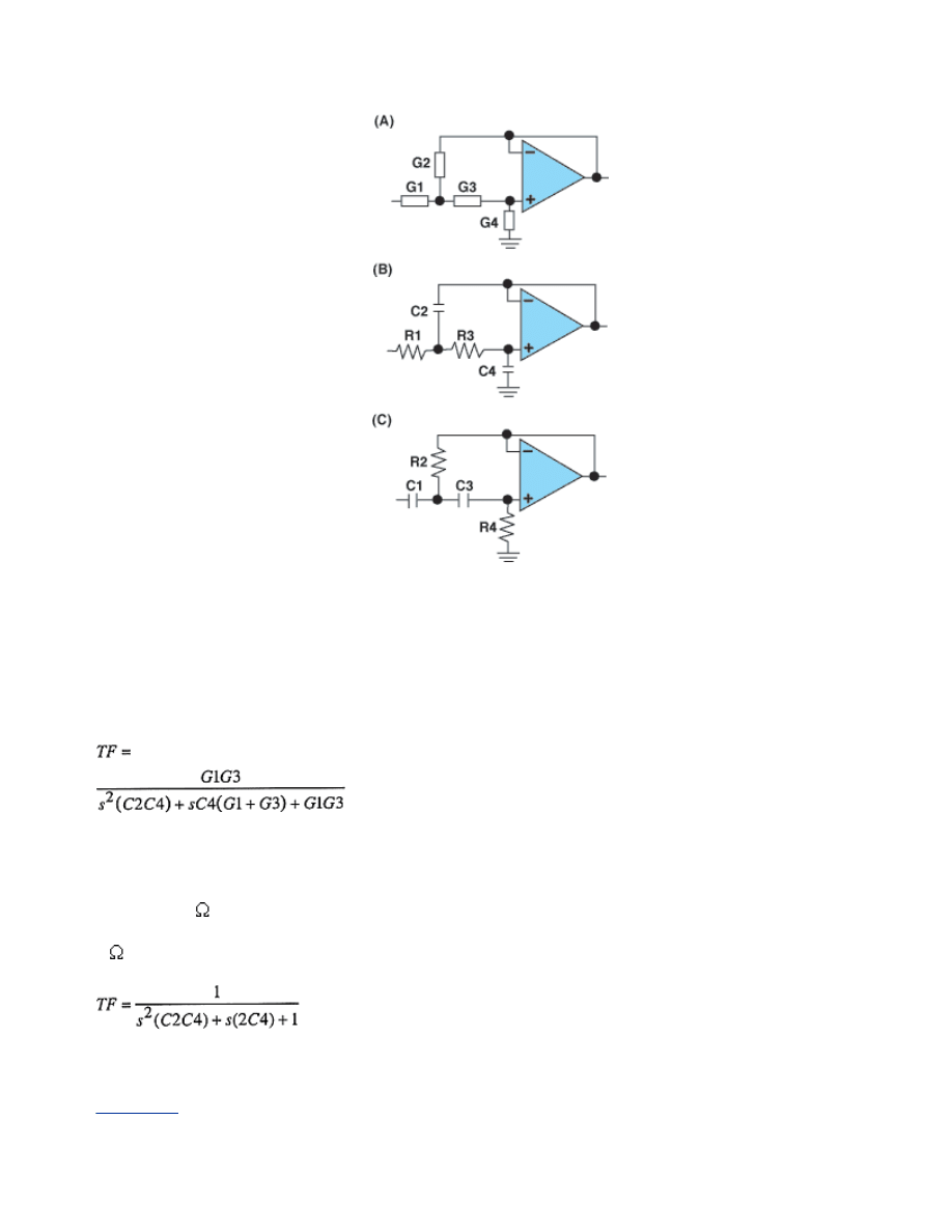
Standard Filter Blocks

The generic filter structure (see
Figure 1A) lets you realize a high-
pass or low-pass implementation
by substituting capacitors or
resistors in place of components
G1–G4. Considering the effect of
these components on the op-amp
feedback network, you can easily
derive a low-pass filter by making G2/G4 into capacitors and G1/G3
into resistors (see Figure 1B). The opposite yields a high-pass
implementation (see Figure 1C).

The transfer function for the low-pass filter (see Figure 1B) is:

This equation is simpler with conductances. Replace the capacitors
with a conductance of sC and the resistors with a conductance of G.
If this looks complicated, you can normalize the equation. Set the
resistors to 1 or the capacitors to 1 F, and change the surrounding
components to fit the response. Thus, with all resistor values equal to
1 , the low-pass transfer function is:

This transfer function describes the response of a generic, second-
order low-pass filter. You take the theoretical tables of poles (see

Tables 1–7

) that describe the three main filter responses and translate

them into real component values.

Figure 1. By substituting for G1-G4 in the
generic filter block (A), you can implement a
low-pass filter (B) or a high-pass filter (C).

(3)

(4)

Sensors - February 2002 - Demystifying Analog Filter Design

Page 4 of 12

http://www.sensorsmag.com/articles/0202/filter/main.shtml

10/03/2002

The Design Process

To determine the filter type most appropriate for your application,
use the preceding descriptions to select the pass-band performance
needed. The simplest way to determine filter order is to design a
second-order filter stage and then cascade multiple versions of it as
required. Check to see if the result gives the desired stop-band
rejection. Next, proceed with correct pole locations as shown in the
tables at the end of the article. Once pole locations are established,
the component values can soon be calculated.

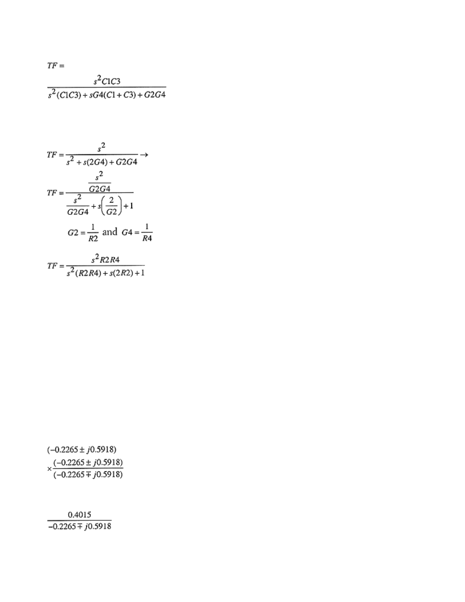
First, transform each pole location into a quadratic expression similar
to that in the denominator of our generic second-order filter. If a
quadratic equation has poles of (a ± jb), then it has roots of (s – a –
jb) and (s – a + jb). When these roots are multiplied together, the

resulting quadratic expression is s

2

– 2as + a

2

+b

2

.

In the pole tables, a is always negative, so for convenience you

declare s

2

+ 2as + a

2

+b

2

and use the magnitude of a regardless of its

sign. To put this into practice, consider a fourth-order Butterworth
filter. The poles and the quadratic expression corresponding to each
pole location are as follows:

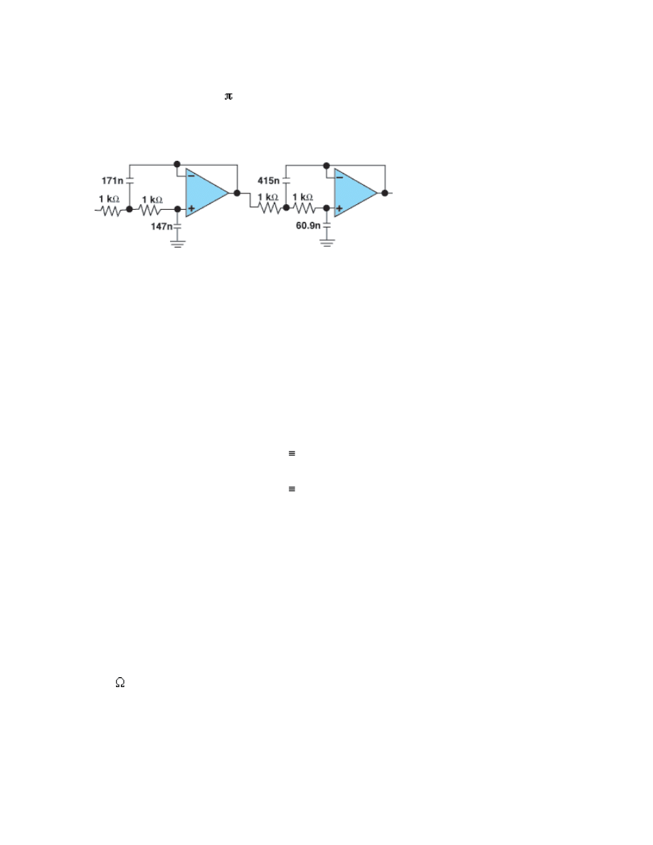
You can design a fourth-order Butterworth low-pass filter with this
information. Simply substitute values from the preceding quadratic
expressions into the denominator of Equation 4. Thus, C2C4 = 1 and
2C4 = 1.8478 in the first filter, which implies that C4 = 0.9239F and
C2 = 1.08F. For the second filter, C2C4 = 1 and 2C4 = 0.7654,
implying that C4 = 0.3827F and C2 = 2.61F. All resistors in both
filters equal 1 . Cascading the two second-order filters yields a
fourth-order Butterworth response with rolloff frequency of 1 rad/s,
but the component values are impossible to find. If the frequency or
component values just given are not suitable, read on.

It so happens that if you maintain the ratio of the reactances to the
resistors, the circuit response remains unchanged. You might
therefore choose 1 k resistors. To ensure that the reactances
increase in the same proportion as the resistances, divide the
capacitor values by 1000.

You still have the perfect Butterworth response, but unfortunately the
rolloff frequency is 1 rad/s. To change the circuit’s frequency
response, you must maintain the ratio of reactances to resistances—
but simply at a different frequency.

Poles (a ± jb)
–0.9239 ± j0.3827
–0.3827 ± j0.9239

Quadratic Expression

s

2

+ 1.8478s + 1

s

2

+ 0.7654s + 1

Sensors - February 2002 - Demystifying Analog Filter Design

Page 5 of 12

http://www.sensorsmag.com/articles/0202/filter/main.shtml

10/03/2002

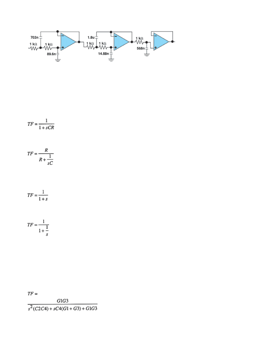
For a rolloff of 1 kHz rather than 1 rad/s, the capacitor value must be
further reduced by a factor of 2 × 1000. Thus, the capacitor’s
reactance does not reach the original (normalized) value until the
higher frequency. The resulting fourth-order Butterworth low-pass
filter with 1 kHz rolloff takes the form of Figure 2.

Using this technique, you can obtain any even-order filter response
by cascading second-order filters. Note, however, that a fourth-order
Butterworth filter is not obtained simply by calculating the
components for a second-order filter and then cascading two such
stages. Instead, two second-order filters must be designed, each with
different pole locations. If the filter has an odd order, you can simply
cascade second-order filters and add an RC network to gain the extra
pole. For example, a fifth-order Chebyshev filter with 1 dB ripple has
the following poles:

To ensure conformance with the generic filter described by Equation
4 and to ensure that the last term equals unity, the first two quadratics
have been multiplied by a constant. Thus, in the first filter, C2C4 =
2.488 and 2C4 = 1.127, which implies that C4 = 0.5635F and C2 =
4.41F. For the second filter, C2C4 = 1.08 and 2C4 = 0.187, which
implies that C4 = 0.0935F and C2 = 11.55F. Earlier, you saw that an
RC circuit has a pole when 1 + sCR = 0: s = –1/CR. If R = 1, then to
obtain the final pole at s = –0.28, you must set C = 3.57F.

Using 1 k resistors, you can normalize for a 1 kHz rolloff
frequency (see Figure 3).

Figure 2. These two nonidentical second-order filter sections form a fourth-order
Butterworth low-pass filter.

Poles

Quadratic Expression

–0.2265 ± j0.5918

s

2

+ 0.453s + 0.402

2.488s

2

+ 1.127s + 1

–0.08652 ± j0.9575

s

2

+ 0.173s + 0.924

1.08s

2

+ 0.187s + 1

–0.2800

See text

Sensors - February 2002 - Demystifying Analog Filter Design

Page 6 of 12

http://www.sensorsmag.com/articles/0202/filter/main.shtml

10/03/2002

Thus, designers can boldly go and design low-pass filters of any
order at any frequency.

All of this theory also applies to the design of high-pass filters.
You’ve seen that a simple RC low-pass filter has the transfer
function of:

Similarly, a simple RC high-pass filter has the transfer function of:

Normalizing these functions to correspond with the normalized pole
tables give:

for low-pass and

for high-pass.

Note that the high-pass pole positions, s, can be obtained by inverting
the low-pass pole positions. Inserting those values into the high-pass
filter block ensures the correct frequency response. To obtain the
transfer function for the high-pass filter block, you need to go back to
the transfer function of the low-pass filter block. Thus, from:

you obtain the transfer function of the equivalent high-pass filter

Figure 3. A fifth-order, 1 dB ripple Chebyshev low-pass filter is constructed from two nonidentical
second-order sections and an output RC network.

(5)

(6)

(7)

(8)

(9)

Sensors - February 2002 - Demystifying Analog Filter Design

Page 7 of 12

http://www.sensorsmag.com/articles/0202/filter/main.shtml

10/03/2002

block by interchanging capacitors and resistors:

Again, life is much simpler if capacitors are normalized instead of
resistors:

Equation 12 is the transfer function of the high-pass filter block. This
time, you calculate resistor values instead of capacitor values. Given
the general high-pass filter response, you can derive the high-pass
pole positions by inverting the low-pass pole positions and
continuing as before. But inverting a complex-pole location is easier
said than done. For example, consider the fifth-order, 1 dB-ripple
Chebyshev filter discussed earlier. It has two pole positions at (–
0.2265 ± j0.5918).

The easiest way to invert a complex number is to multiply and divide
by the complex conjugate, thereby obtaining a real number in the
numerator. You then find the reciprocal by inverting the fraction.

Thus:

gives:

and inverting gives:

(10)

(11)

(12)

(13)

(14)

Sensors - February 2002 - Demystifying Analog Filter Design

Page 8 of 12

http://www.sensorsmag.com/articles/0202/filter/main.shtml

10/03/2002

You can convert the newly derived pole positions to the
corresponding quadratic expression and values calculated as before.
The result is:

From Equation 12, you can calculate the first filter component values
as R2R4 = 0.401 and 2R2 = 0.453, which implies that R2 = 0.227
and R4 = 1.77 . You can repeat the procedure for the other pole
locations.

Because we’ve shown that s =

–1

/

CR

, a simpler approach is to design

for a low-pass filter by using suitable low-pass poles and then treat
every pole in the filter as a single RC circuit. To invert each low-pass
pole to obtain the corresponding high-pass pole, simply invert the
value of CR. Once you’ve obtained the high-pass pole locations, you
ensure the correct frequency response by interposing the capacitors
and resistors.

You calculated a normalized capacitor value for the low-pass
implementation, assuming that R = 1 . Hence, the value of CR
equals the value of C, and the reciprocal of the value of C is the high-
pass pole. Treating this pole as the new value of R yields the
appropriate high-pass component value.

Considering again the fifth-order, 1 dB ripple Chebyshev low-pass
filter, the calculated capacitor values are C4 = 0.5635F and C2 =
4.41F. To obtain the equivalent high-pass resistor values, invert the
values of C (to obtain high-pass pole locations) and treat these poles
as the new normalized resistor values: R4 = 1.77 and R2 = 0.227.
This approach provides the same results as does the more formal
method mentioned earlier.

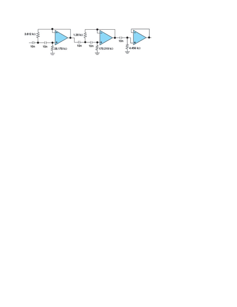
Thus, the circuit in Figure 3 can be converted to a high-pass filter
with 1 kHz rolloff by inverting the normalized capacitor values,
interposing the resistors and capacitors, and scaling the values
accordingly. Earlier, we divided by 2 fR to normalize the low-pass
values. The scaling factor in this case is 2 fC, where C is the
capacitor value and f is the frequency in hertz. The resulting circuit is
shown in Figure 4.

(15)

Poles (a ± jb)
–0.564 ± j1.474

Quadratic Expression

s

2

+ 1.128s + 2.490

0.401s

2

+ 0.453s + 1

Sensors - February 2002 - Demystifying Analog Filter Design

Page 9 of 12

http://www.sensorsmag.com/articles/0202/filter/main.shtml

10/03/2002

Conclusion

By using the methods described here, you can design low-pass and
high-pass filters with response at any frequency. Band-pass and
band-stop filters can also be implemented (with single op amps) by
using techniques similar to those shown, but those applications are
beyond the scope of this article. You can, however, implement band-
pass and band-stop filters by cascading low-pass and high-pass
filters.

This article promises to be your guide through the wilderness, your
defense against the headhunters, and your key to the analog kingdom.

Figure 4. Transposing resistors and capacitors in the circuit in Figure 3 yields a fifth-order, 1 dB
ripple, Chebyshev high-pass filter.

TABLE 1

Butterworth Pole Locations

Order

Real

-a

Imaginary

+/-jb

2

0.7071

0.7071

3

0.5000
1.0000

0.8660

4

0.9239
0.3827

0.3827
0.9239

5

0.8090
0.3090
1.0000

0.5878
0.9511

6

0.9659
0.7071
0.2588

0.2588
0.7071
0.9659

7

0.9010
0.6235
0.2225
1.0000

0.4339
0.7818
0.9749

8

0.9808
0.8315
0.5556
0.1951

0.1951
0.5556
0.8315
0.9808

9

0.9397
0.7660
0.5000
0.1737
1.0000

0.3420
0.6428
0.8660
0.9848

10

0.9877
0.8910
0.7071

0.1564
0.4540
0.7071

TABLE 2

Bessel Pole Locations

Order

Real

-a

Imaginary

+/-jb

2

1.1030

0.6368

3

1.0509
1.3270

1.0025

4

1.3596
0.9877

0.4071
1.2476

5

1.3851
0.9606
1.5069

0.7201
1.4756

6

1.5735
1.3836
0.9318

0.3213
0.9727
1.6640

7

1.6130
1.3797
0.9104
1.6853

0.5896
1.1923
1.8375

8

1.7627
0.8955
1.3780
1.6419

0.2737
2.0044
1.3926
0.8253

9

1.8081
1.6532
1.3683
0.8788
1.8575

0.5126
1.0319
1.5685
2.1509

Sensors - February 2002 - Demystifying Analog Filter Design

Page 10 of 12

http://www.sensorsmag.com/articles/0202/filter/main.shtml

10/03/2002

0.7071
0.4540
0.1564

0.7071
0.8910
0.9877

TABLE 3

0.01 dB Chebyshev Pole

Locations

Order

Real

-a

Imaginary

+/-jb

2

0.6743

0.7075

3

0.4233
0.8467

0.8663

4

0.6762
0.2801

0.3828
0.9241

5

0.5120
0.1956
0.6328

0.5879
0.9512

6

0.5335
0.3906
0.1430

0.2588
0.7072
0.9660

7

0.4393
0.3040
0.1085
0.4876

0.4339
0.7819
0.9750

8

0.4268
0.3618
0.2418
0.0849

0.1951
0.5556
0.8315
0.9808

9

0.3686
0.3005
0.1961
0.0681
0.3923

0.3420
0.6428
0.8661
0.9848

TABLE 4

0.1 dB Chebyshev Pole

Locations

Order

Real

-a

Imaginary

+/-jb

2

0.6104

0.7106

3

0.3490
0.6979

0.8684

4

0.2177
0.5257

0.9254
0.3833

5

0.3842
0.1468
0.4749

0.5884
0.9521

6

0.3916
0.2867
0.1049

0.2590
0.7077
0.9667

7

0.3178
0.2200
0.0785
0.3528

0.4341
0.7823
0.9755

8

0.3058
0.2592
0.1732
0.0608

0.1952
0.5558
0.8319
0.9812

9

0.2622
0.2137
0.1395
0.0485
0.2790

0.3421
0.6430
0.8663
0.9852

TABLE 5

0.25 dB Chebyshev Pole

Locations

Order

Real

-a

Imaginary

+/-jb

2

0.5621

0.7154

3

0.3062
0.6124

0.8712

4

0.4501
0.1865

0.3840
0.9272

5

0.3247
0.1240
0.4013

0.5892
0.9533

6

0.3284
0.2404
0.0880

0.2593
0.7083
0.9675

7

0.2652

0.4344

TABLE 6

0.5 dB Chebyshev Pole

Locations

Order

Real

-a

Imaginary

+/-jb

2

0.5129

0.7225

3

0.2683
0.5366

0.8753

4

0.3872
0.1605

0.3850
0.9297

5

0.2767
0.1057
0.3420

0.5902
0.9550

6

0.2784
0.2037
0.0746

0.2596
0.7091
0.9687

7

0.2241

0.4349