Division of Engineering Fundamentals , Copyright 1999 by J.C. Malzahn Kampe 1 / 21
Virginia Polytechnic Institute & State University EF1015 Revised Fall 2000
_____________________________________________________

MATLAB Programming

When we use the phrase “computer solution,” it should be understood that a computer
will only follow directions; the “solution” part of that phrase still resides with the person
directing the machine. Developing an algorithm to solve a problem is the first step in a
“computer solution.” The computer must then be given every procedural step, in the
proper order, to accomplish the task that we require of it. With that in mind, an
appreciation of how explicit we must be with our directions is helpful. Consider a young,
barefoot child. If you tell this child to “put on the shoes” that you have set out, the child
is very likely to come back to you with the shoes on, carrying socks in hand. In
retrospect, the child has accomplished the task you had put before him. Had you also
wanted socks on his feet, surely you would have told him.

In an effort to understand the three aspects of programming that we will cover
(sequential, selection or decision, and repetition) it is useful to have an example to
follow. In the following sections, we will consider these four problem statements.

1. Prepare a flowchart and MATLAB program that will calculate the area and

circumference of a circle, allowing the radius to be an input variable, and output
radius, area, and circumference.

2. Prepare a flowchart and MATLAB program that will calculate the area and

circumference of a circle, allowing the radius to be an input variable, and output
radius, area, and circumference only if the area of the circle is greater than 20.

3. Prepare a flowchart and MATLAB program that will calculate the area and

circumference of ten circles, allowing radius to be an input variable, and output
radius, area, and circumference only if the area of the circle is greater than 20. The
number of circles that do not have an area greater than 20 should also be output.

4. Prepare a flowchart and MATLAB program that will calculate the area and

circumference of any number of circles, allowing radius to be an input variable, and
output radius, area, and circumference only if the area of the circle is greater than 20.
The number of circles examined that do not have an area greater than 20 should also
be output.

Problem 1: Sequential

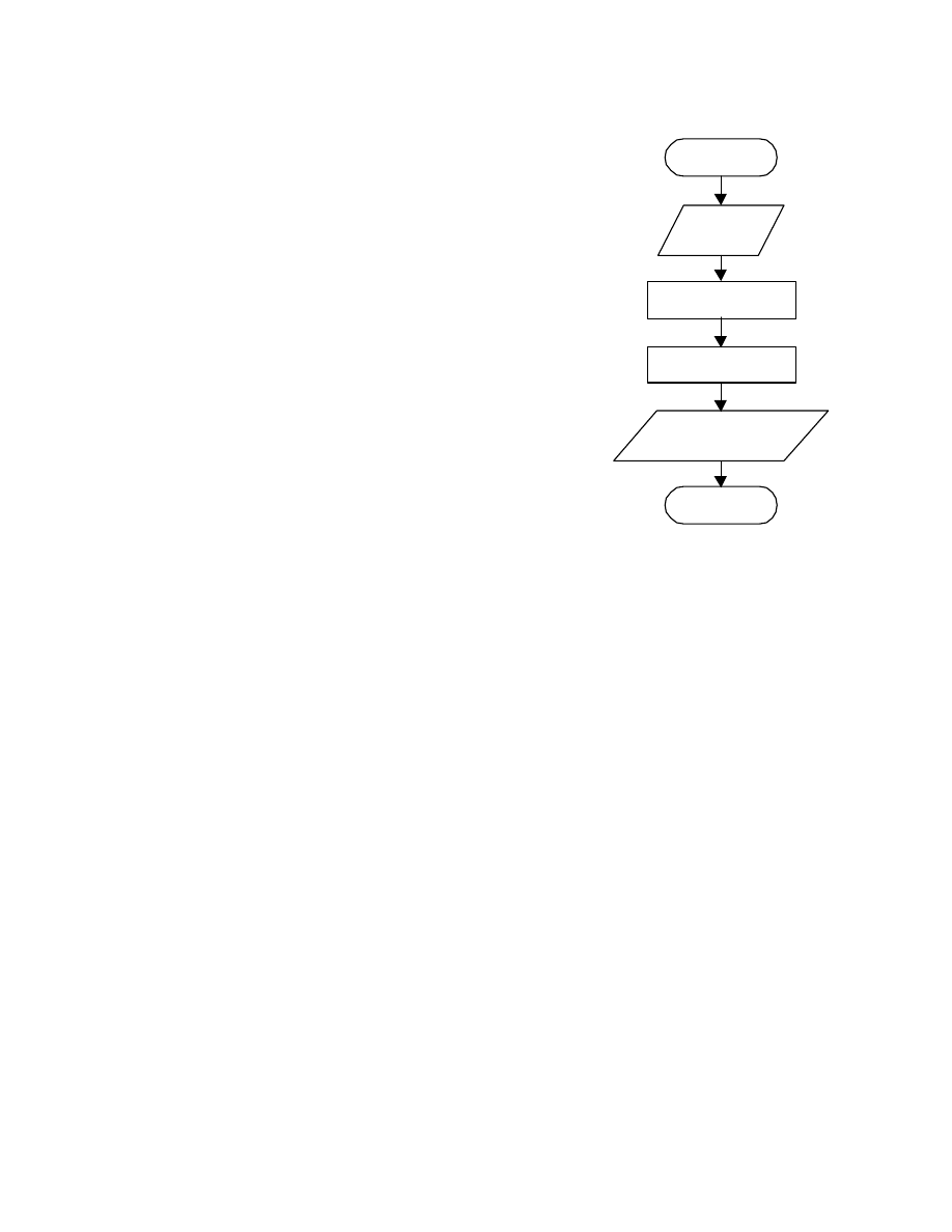
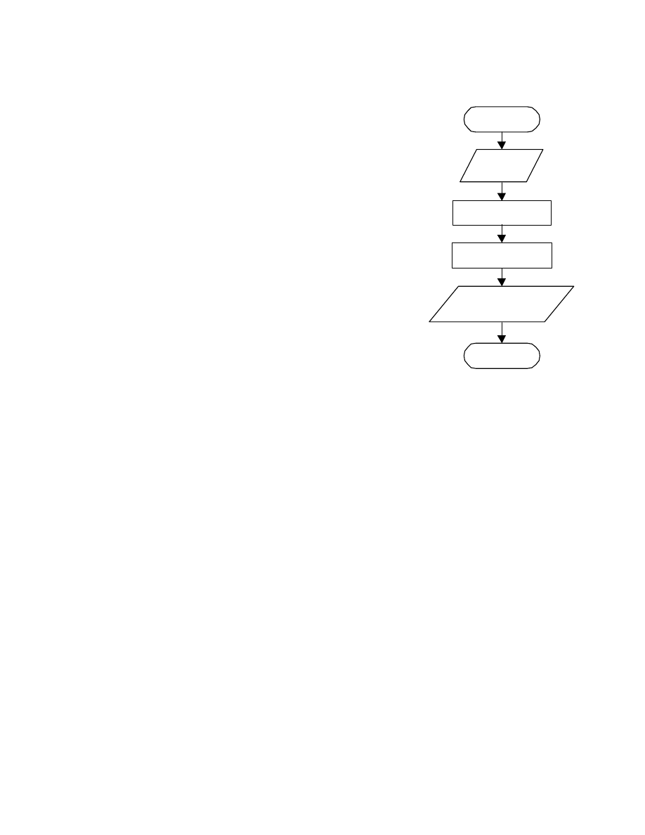
The solution algorithm for Problem 1 involves a sequence of procedures that follows a
single logic flow path from “START” to “STOP”. The flowchart and program are shown
in Figure 1.

Division of Engineering Fundamentals , Copyright 1999 by J.C. Malzahn Kampe 2 / 21
Virginia Polytechnic Institute & State University EF1015 Revised Fall 2000
_____________________________________________________

% This program will calculate the
%

area and circumference of a circle,

%

allowing the radius as an input.

R = input('Please enter the radius: ');

AREA = pi * R^2;

CIRC = 2.0 * pi * R;

fprintf('\n Radius = %f units',R)
fprintf('\n Area = %f square units', AREA)

fprintf('\n Circumference = %f units\n', CIRC)

Figure 1. A MATLAB program (a script m-file named Prob1) and the corresponding
flowchart for Problem 1.
________________________________________________________________________

At this point you may have many questions about how we get to the contents of Figure 1,
so let’s go through that first.

After reading Problem 1 above, we must first develop an approach (algorithm) to obtain
what the problem statement requires. Our solution algorithm is documented with the
flowchart that appears in Figure 1. The flowchart is produced using the drawing features
available in MS Word under “Flowchart” in the “AutoShapes” menu of the lower toolbar.
Next we translate the flowcharted algorithm to a computer program (code) that
MATLAB can interpret and execute. This program appears on the left in Figure 1. In
order to produce this code, we open MATLAB, and go to the “File” menu in the upper
toolbar, and select “New.” Of the options that come up, we then select “M-File;” this
opens the MATLAB “Editor/Debugger” window. Once this window is open, we can
type in our program, edit the program, and save it to our “Work” folder.

Now take a look at the correspondence between the flowchart and the code in Figure 1.
The first thing to note is that there are no MATLAB commands in the code to “START”
or “STOP” the program. The script file begins with statements that have been
commented out of the executable statements by placing “%” in the first position on those
lines. The “%” tells MATLAB that what follows on that line can be ignored during
program run. We use the comment lines to describe what the program does. Also, if, in
the command window, we type

START

STOP

INPUT

R

OUTPUT

R, AREA, CIRC

AREA =

π

R

2

CIRC = 2.0

π

R

Division of Engineering Fundamentals , Copyright 1999 by J.C. Malzahn Kampe 3 / 21
Virginia Polytechnic Institute & State University EF1015 Revised Fall 2000
_____________________________________________________

» help Prob1

This program will calculate the

area and circumference of a circle,

allowing the radius as an input.

we see that MATLAB responds with those comments that begin the script file named
Prob1.

Below the comments, the first executable statement in the file identifies “R” as an input
variable. In the statement

R = input('Please enter the radius: ');

we tell MATLAB to print “Please enter the radius:” to the screen as a prompt to the user
that the radius value must be entered. MATLAB accepts the entered value, and stores it
under the variable named “R.” The “;” at the end of the statement suppresses the
MATLAB echo of the value entered. This input value assignment statement corresponds
to the “INPUT” symbol in the flowchart.

Beneath the input statement of the code are two value assignment statements.

AREA = pi * R^2;

CIRC = 2.0 * pi * R;

These correspond to the two process symbols in the flowchart; they use the value stored
as “R” in calculations and assign the calculation results to “AREA” and “CIRC.” It is
important to remember the form that value assignment statements require. Only a single
variable with no operators may appear on the left of the equal sign, and all variables on
the right of the equal sign must have a current assigned value.

Looking at the flowchart, our last order of business is to output the values for “R,”
“AREA,” and “CIRC.” In the code shown in Figure 1, we use fprintf statements to
accomplish this.

fprintf('\n Radius = %f units',R)
fprintf('\n Area = %f square units', AREA)
fprintf('\n Circumference = %f units\n', CIRC)

Using these statements allows us to format our output. In other words, these commands
let us tell MATLAB exactly how we want our values for “R,” “AREA,” and “CIRC”
printed to the screen. Within the parentheses of the first fprintf statement, the “\n” is a
carriage return command that tells MATLAB to start printing on a new line. MATLAB
interprets what follows in that statement as a character string that contains a format field
for a number (the “%f”), and that the number to be placed at the position designated by
“%f” is stored under the variable named “R.” Note that the carriage return, the text, and

Division of Engineering Fundamentals , Copyright 1999 by J.C. Malzahn Kampe 4 / 21
Virginia Polytechnic Institute & State University EF1015 Revised Fall 2000
_____________________________________________________

the format field are enclosed within single quote marks, and the variable name (which
stores the value) specified to fill the number format field is listed outside the quotes, but
before the closing parenthesis. Note, also, that a comma separates the format string (i.e.,
what is contained within the single quotes) and the variable name that stores the value to
be placed in the number format field. It was not necessary to use three different fprintf
statements because you can output more than one argument with fprintf statements.
Three were used to keep the length of the code statements short enough to fit within
Figure 1. The number field was specified as a fixed point formatted field by use of
“%f”. Use “%e” for exponential format, and “%g” when either fixed point or
exponential format (which ever is shorter) is acceptable. We can also tell MATLAB how
many places past the decimal point we would like, as in “%.3f”, which specifies that
three places after the decimal be displayed in fixed point format. Now, if you do not
wish to format your output, you can use MATLAB’s disp command, which has the
following syntax

disp(argument)

where “argument” is replaced with a single variable name, or with a character string (that
cannot contain any format fields) enclosed within single quotes. The disp statement will
accept only one argument, so for our flowchart in Figure 1, three disp statements would
be required just to output the variables, with no annotating text.

Now that we understand the translation of the flowchart to code, how is the code
executed? If you are in the “Editor/Debugger” window with the script m-file open, you
can choose “Run” from the options in the “Tools” pull-down menu, and the command
window will show execution of the program.

» Please enter the radius: 32

Radius = 32.000000 units
Area = 3216.990877 square units
Circumference = 201.061930 units

If you are in the command window, you can enter the script m-file name at the prompt.

» Prob1
Please enter the radius: 32

Radius = 32.000000 units
Area = 3216.990877 square units
Circumference = 201.061930 units
»

Division of Engineering Fundamentals , Copyright 1999 by J.C. Malzahn Kampe 5 / 21
Virginia Polytechnic Institute & State University EF1015 Revised Fall 2000
_____________________________________________________

» Prob1
Please enter the radius: 5

Radius = 5.000000 units
Area = 78.539816 square units
Circumference = 31.415927 units
»

Problem 2: Selection / Decision

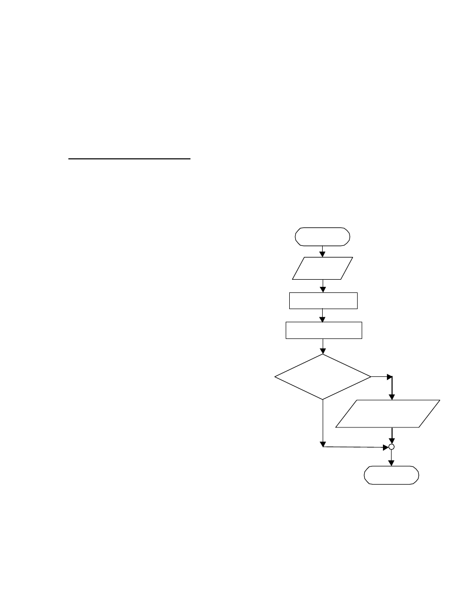
The solution to Problem 2 involves a decision on whether the radius, area and
circumference values should be printed. This decision to output is based on whether the
area value exceeds 20. Figure 2 shows a MATLAB program and flowcharted algorithm
that produces the results requested in Problem 2.

% This program will calculate the
%

area and circumference of a circle,

%

allowing the radius as an input,

%

but will only provide output if the

%

area exceeds 20.

R = input('Please enter the radius: ');

AREA = pi * R^2;

CIRC = 2.0 * pi * R;

if AREA > 20.0

fprintf('\n Radius = %f units',R)
fprintf('\n Area = %f square units', AREA)

fprintf('\n Circumference = %f units\n', CIRC)

end

Figure 2. A MATLAB program (a script m-file named Prob2) and the corresponding
flowchart for Problem 2.
________________________________________________________________________

START

INPUT

R

OUTPUT

R, AREA, CIRC

AREA =

π

R

2

if

AREA > 20.0

STOP

TRUE

FALSE

CIRC = 2.0

π

R

Division of Engineering Fundamentals , Copyright 1999 by J.C. Malzahn Kampe 6 / 21
Virginia Polytechnic Institute & State University EF1015 Revised Fall 2000
_____________________________________________________

The difference between what you see in Figures 1 and 2 involves the decision to output.
In the algorithm flowchart of Figure 2, we see that the decision to output is based on the
value of AREA. If AREA exceeds 20, the logic flow path selected as the exit from the
decision diamond is the

TRUE

path and will execute output. If AREA is not greater than

20, the output symbol is bypassed in the selected logic flow along the

FALSE

path. In the

corresponding code shown in Figure 2, we see that the fprintf statements that produce
output have been enclosed within an “if” structure. The “if” structure begins with an if
statement, which is followed by the statements to be executed when the conditions of the
if statement (here, AREA > 20) are met. The “if” structure is closed by the end
statement, which designates where the

TRUE

and

FALSE

paths recombine.

To verify that the code executes properly, we should run the script m-file Prob2.

» Prob2
Please enter the radius: 32

Radius = 32.000000 units
Area = 3216.990877 square units
Circumference = 201.061930 units
»
» Prob2
Please enter the radius: 2
»
» Prob1
Please enter the radius: 2

Radius = 2.000000 units
Area = 12.566371 square units
Circumference = 12.566371 units
»

We see that a radius value of 2 produces no output when entered as Prob2 is run because
AREA (determined as 12.566371 from Prob1 output) is not greater than 20.

Problem 3: Repetition (“for” Loop)

Two features of Problem 3 add twists to what we have done so far. The first is the need
to repeat certain procedural steps in the solution algorithm. This repetition is
accomplished by looping the logic flow path. The second twist involves the requirement
to count the number of circles (in the 10-circle run) that do not meet the area criterion for
output. This requirement modifies the “if” structure discussed under Problem 2. A
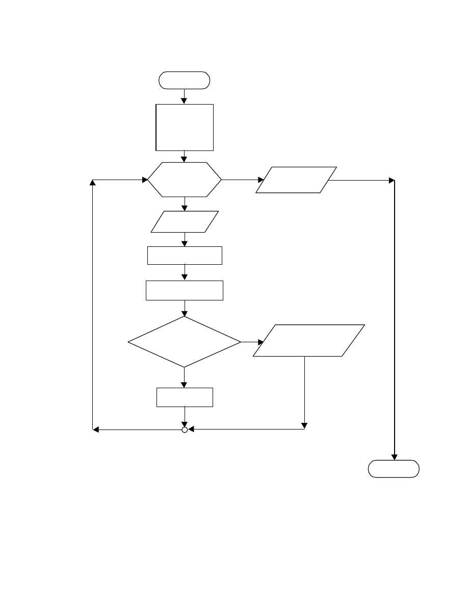
flowchart and MATLAB program that produce the results requested in Problem 3 are
shown in Figures 3a and 3b, respectively.

Division of Engineering Fundamentals , Copyright 1999 by J.C. Malzahn Kampe 7 / 21
Virginia Polytechnic Institute & State University EF1015 Revised Fall 2000
_____________________________________________________

Figure 3a. A flowchart that documents a solution algorithm for Problem 3.
________________________________________________________________________

STOP

OUTPUT

R, AREA, CIRC

OUTPUT

N

True

START

for

J from 1 to

10 by 1

INPUT

R

AREA =

π

· R

2

N = 0
R = 0.0
AREA = 0.0
CIRC = 0.0

if

AREA > 20.0

N = N + 1

False

CIRC = 2.0 ·

π

· R

Division of Engineering Fundamentals , Copyright 1999 by J.C. Malzahn Kampe 8 / 21
Virginia Polytechnic Institute & State University EF1015 Revised Fall 2000
_____________________________________________________

% This program will calculate the
%

area and circumference of ten circles,

%

allowing the radius as an input,

%

but will only provide output for circles

%

with an area that exceeds 20.

N = 0; R = 0.0; AREA = 0.0; CIRC = 0.0;

for J = 1:1:10

R = input('Please enter the radius: ');
AREA = pi * R^2;
CIRC = 2.0 * pi * R;

if AREA > 20.0
fprintf('\n Radius = %f units',R)
fprintf('\n Area = %f square units', AREA)
fprintf('\n Circumference = %f units\n', CIRC)
else
N = N + 1;

end

end

fprintf('\n Number of circles that do not have area > 20: %.0f \n', N)

Figure 3b. A MATLAB program (script m-file named Prob3) for Problem 3 that
corresponds to the flowchart of Figure 3a.
________________________________________________________________________

Take a close look at Figure 3a; the flowchart there appears substantially different from
the flowchart shown in Figure 2. We should examine the differences, one at a time, in
order to gain an understanding of what the new requirements of Problem 3’s solution
entail in terms of flowcharting and subsequent programming.

The most substantial change between the two flowcharts is the looping of the logic flow
path. This is accommodated, in the flowchart, by introduction of the looping hexagon
symbol (which contains “for J from 1 to 10 by 1”) and the return of logic flow back to the
hexagon after the decision structure executes. The statement inside the hexagon indicates
that a predetermined number of executions of the loop will occur, which is controlled by
the value of “J.” The first time the hexagon symbol is entered, “J” is set to 1, and then
compared to the ending value for “J,” which here is 10. If the current value of “J” does
not exceed its ending value (here 10), the loop will execute. That is, logic flow will move
down through the INPUT symbol, through the two process blocks, through the decision
diamond and along the path selected by the value of “AREA”, and then back to the loop
hexagon. Upon return to the hexagon, “J” will increment by 1 to become 2, and then be
compared to 10. As 2 does not exceed 10, the loop will execute again. This repeats until

Division of Engineering Fundamentals , Copyright 1999 by J.C. Malzahn Kampe 9 / 21
Virginia Polytechnic Institute & State University EF1015 Revised Fall 2000
_____________________________________________________

“J” becomes 11. When 11 is compared to the ending value for “J” (which is 10), logic
flow exits the loop because the looping conditions are no longer met.

The loop depicted in Figure 3 is called a “for” loop. A “for” loop is used when the
number of times a procedure must be repeated is known, either by the programmer or by
the user. In the statement within the hexagon, “for J from 1 to 10 by 1,” any of the
numbers that specify the starting value, the ending value, or the incrementing value, can
be replaced by a variable name, which, in turn, can be allowed as input. For example, if
we put “for J from 1 to NUMBER by 1” in the hexagon, then we could let the user input
how many circles were to be evaluated by entering that quantity as “NUMBER” in an
input value assignment statement that preceded the loop.

Now we turn our attention to the process block below the decision diamond. This
process block contains a counting value assignment statement (N = N + 1) that counts the
number of circles that do not meet the area criterion for output. In the flowchart of
Figure 3, we can see that if “AREA > 20.0” is false, then the selected logic flow path will
execute “N = N + 1.” If “AREA > 20.0” is true, the counting statement is bypassed.
Note that each time “N = N + 1” executes, the value of “N” increases by 1, thus counting
the executions of the “N = N + 1” statement, and hence the number of times that “AREA
> 20.0” is false.

Another change in the flowcharts as we move from Problem 2 to Problem 3 is the
addition of a new process block in Figure 3. This process block contains value
assignment statements that set the variables N, R, AREA, and CIRC equal to zero, and is
placed just below “START.” This procedure is called “initialization” of variables. It is
often only a safety feature that experienced programmers use when solution algorithms
become complex, but sometimes it is required in the logic of the algorithm. In the case of
Problem 3, the initialization of “R”, “AREA”, and “CIRC” is not required, but it is
necessary that we initialize “N” at a value of zero. This is so for two reasons. The first
reason that “N” must be set to zero involves the counting statement “N = N + 1.” In
execution of this statement, MATLAB will always need a “current” value of “N” to
evaluate the right side of the statement (i.e., N + 1). The first time the statement
executes, the “new” value of N becomes 1. If “N” is not initialized at zero, “N = N + 1”
cannot keep a proper count of the number of circles that do not meet the area criterion for
output.

The second reason we initialize N at zero is because a user may have ten circles, all of
which do meet the area criterion. If this happens, then when loop execution is completed,
MATLAB will need a numeric value for “N” in order to execute the “N” output required
upon loop exit. If “N” has not been defined (i.e., given a numeric value), MATLAB will
respond with an error statement. The value “N” should be storing in this event is zero,
because all circles will have met the area criterion. It should be noted that zero is not
always the appropriate value to use for variable initialization. In the case of Problem 3,
however, zero works for the logic of the algorithm.

Division of Engineering Fundamentals , Copyright 1999 by J.C. Malzahn Kampe 10 / 21
Virginia Polytechnic Institute & State University EF1015 Revised Fall 2000
_____________________________________________________

We are now ready to look at the MATLAB program (Figure 3b) that corresponds to the
flowchart in Figure 3a. Below the comments, we see the value assignment statements
that initialize “N,” “R,” “AREA,” and “CIRC.” Although these are typed in on a single
line, MATLAB reads them as four separate statements because the semicolons that
suppress the echoes also act as delimiters. Next, the for loop opens with

for J = 1:1:10

and closes with the second end statement. You should next notice that the “if” structure
contains two new statements, else and N = N + 1.

if AREA > 20.0

fprintf('\n Radius = %f units',R)

fprintf('\n Area = %f square units', AREA)
fprintf('\n Circumference = %f units\n', CIRC)
else
N = N + 1;
end

In this “if” structure, the statements to be executed when “AREA > 20.0” is true follow
directly below the if statement. Those statements that are executed only when “AREA >
20.0” is false are placed directly below an else statement, and the “if” structure is closed
with the first end statement. You should note that, for Problem 2 (where we had nothing
to execute when “AREA > 20.0” was false), an else statement was not required. The
function of the else here is to ensure that the counting statement (N = N + 1) is bypassed
when “AREA > 20.0” is true, and that “N = N + 1” executes when “AREA > 20.0” is
false. During script file run, if “AREA > 20.0” is true, MATLAB will execute all
statements that follow the if until it reaches the else, and all statements between else and
end are skipped. If “AREA > 20.0” is false, MATLAB will skip all statements until it
reaches the else, and then resume execution. You should be aware that “if” structures can
be nested so that elseif statements are often used in programming to provide third, fourth,
and more alternate logic flow paths.

The last thing to observe in the code shown in Figure 3b is the final fprintf statement.
This provides the output of “N,” the number of circles that do not meet the area criterion.
A verification of the script file Prob3 is shown below in the MATLAB output for a run
from the command window.

Division of Engineering Fundamentals , Copyright 1999 by J.C. Malzahn Kampe 11 / 21
Virginia Polytechnic Institute & State University EF1015 Revised Fall 2000
_____________________________________________________

» Prob3
Please enter the radius: 1
Please enter the radius: 2
Please enter the radius: 3

Radius = 3.000000 units
Area = 28.274334 square units
Circumference = 18.849556 units
Please enter the radius: 4

Radius = 4.000000 units
Area = 50.265482 square units
Circumference = 25.132741 units
Please enter the radius: 5

Radius = 5.000000 units
Area = 78.539816 square units
Circumference = 31.415927 units
Please enter the radius: 6

Radius = 6.000000 units
Area = 113.097336 square units
Circumference = 37.699112 units
Please enter the radius: 7

Radius = 7.000000 units
Area = 153.938040 square units
Circumference = 43.982297 units
Please enter the radius: 8

Radius = 8.000000 units
Area = 201.061930 square units
Circumference = 50.265482 units
Please enter the radius: 9

Radius = 9.000000 units
Area = 254.469005 square units
Circumference = 56.548668 units
Please enter the radius: 10

Radius = 10.000000 units
Area = 314.159265 square units
Circumference = 62.831853 units

Number of circles that do not have area > 20: 2

Division of Engineering Fundamentals , Copyright 1999 by J.C. Malzahn Kampe 12 / 21
Virginia Polytechnic Institute & State University EF1015 Revised Fall 2000
_____________________________________________________

Problem 4: Repetition (“while” Loop)

In Problem 4, it is required that the loop executes for as many times as required by the
user. Now, as discussed above, we could use a “for” loop, and have the user count the
number of circles to be evaluated. This is no great task when only a few executions are
required. However, if the user has a large number of circles to evaluate, counting them is
not an option. Further, if interrupted by something more pressing, the user may not be
able to run all the circles in one session. In efforts to create a “user friendly” program,
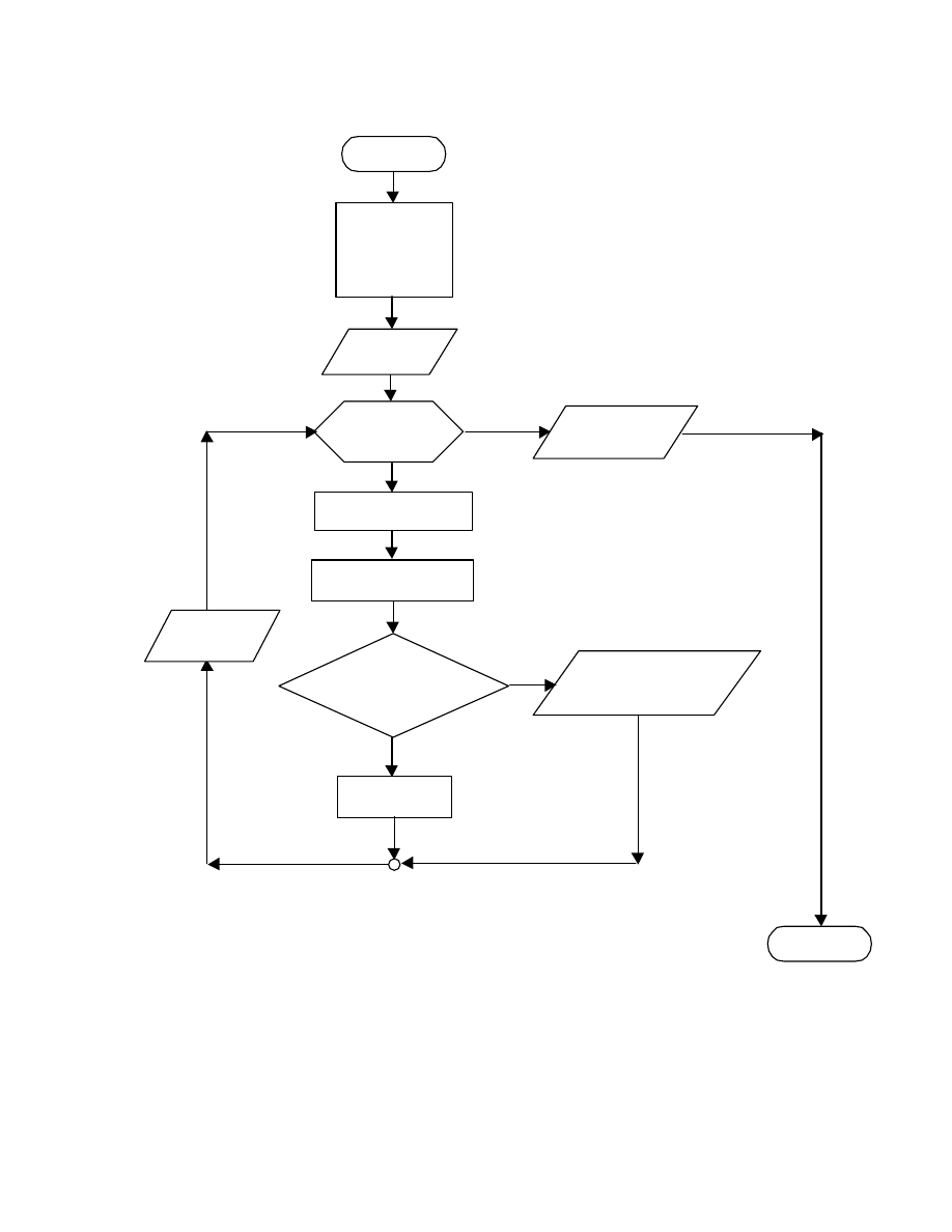
these situations should be anticipated. A flowchart that documents an algorithm for
Problem 4 is shown in Figure 4a. The corresponding MATLAB script m-file is provided
in Figure 4b.

The main distinction between the flowcharts for Problems 3 and 4 is the type of loop
employed. Problem 4 requires a repeat of procedural steps for as many times as the user
wishes to run circles. In this case, we use a while loop because we cannot predetermine
how many times the loop should execute. The looping condition in the while loop of
Problem 4 is based on the value of “R.” When “R” is positive, the loop executes. This
makes physical sense, as any circle that should be evaluated will have a positive radius.
Now, to accommodate the change in the logic used to control the number of loop
executions, we need two other modifications in our flowchart and program. First, we
must input a value for “R” before we enter the loop, so that MATLAB can obtain a non-
zero numeric value for “R” before it reaches the while loop statement. The second
modification we need to make is moving the input of “R” that sits within the loop. This
second input statement must occur just prior to re-entering the loop hexagon. This new
position ensures that “R” is evaluated as greater than zero before any calculations are
executed (in case the user enters zero to quit). This input position also ensures that, when
the user enters zero for R in order to quit, the circle with R = 0 is not counted among
those circles for which “AREA > 20.0” is false.

In the MATLAB code that corresponds to Figure 4a (found in Figure 4b), we see the
implementation of the required changes to our solution algorithm. We find an input
statement

R = input('Please enter the radius (enter 0 to quit): ');

which precedes the while statement

while R > 0.0

that starts the loop. Also, the input statement for “R” within the loop now follows the
end that closes the “if” structure.

Division of Engineering Fundamentals , Copyright 1999 by J.C. Malzahn Kampe 13 / 21
Virginia Polytechnic Institute & State University EF1015 Revised Fall 2000
_____________________________________________________

Figure 4a. A flowchart that documents a solution algorithm for Problem 4.
________________________________________________________________________

START

STOP

while

R > 0.0

OUTPUT

R, AREA, CIRC

OUTPUT

N

AREA =

π

· R

2

N = 0
R = 0.0
AREA = 0.0
CIRC = 0.0

if

AREA > 20.0

N = N + 1

True

False

INPUT

R

INPUT

R

CIRC = 2.0 ·

π

· R

Division of Engineering Fundamentals , Copyright 1999 by J.C. Malzahn Kampe 14 / 21
Virginia Polytechnic Institute & State University EF1015 Revised Fall 2000
_____________________________________________________

% This program will calculate the
%

area and circumference of circles,

%

allowing the radius as an input,

%

but will only provide output for circles

%

with an area that exceeds 20.

N = 0; R = 0.0; AREA = 0.0; CIRC = 0.0;

R = input('Please enter the radius (enter 0 to quit): ');

while R > 0.0

AREA = pi * R^2;
CIRC = 2.0 * pi * R;

if AREA > 20.0
fprintf('\n Radius = %f units',R)
fprintf('\n Area = %f square units', AREA)
fprintf('\n Circumference = %f units\n', CIRC)
else
N = N + 1;
end

R = input('Please enter the radius (enter 0 to quit): ');

end

fprintf('\n Number of circles that do not have area > 20: %.0f \n', N)

Figure 4b. A MATLAB program (script m-file named Prob4) for Problem 4 that
corresponds to the flowchart in Figure 4a.
________________________________________________________________________

The last thing to note about the code in Figure 4b is the user prompt in the input
statements. Because our code is set up to allow the user to control execution of the loop,
we must provide the user with some instructions on how to exit the program. Hence,
“enter 0 to quit” is added to the prompt that requests an input for “R.”

Division of Engineering Fundamentals , Copyright 1999 by J.C. Malzahn Kampe 15 / 21
Virginia Polytechnic Institute & State University EF1015 Revised Fall 2000
_____________________________________________________

Verification of the code in Figure 4b is shown below in the MATLAB output for a Prob4
run from the command window.

» Prob4
Please enter the radius (enter 0 to quit): 0.5
Please enter the radius (enter 0 to quit): 1
Please enter the radius (enter 0 to quit): 2
Please enter the radius (enter 0 to quit): 3

Radius = 3.000000 units
Area = 28.274334 square units
Circumference = 18.849556 units
Please enter the radius (enter 0 to quit): 4

Radius = 4.000000 units
Area = 50.265482 square units
Circumference = 25.132741 units
Please enter the radius (enter 0 to quit): 0

Number of circles that do not have area > 20: 3
»

MATLAB Function m-files

To make this document complete as a tutorial on MATLAB programming, we should
address the syntax and use of MATLAB function m-files. You have been using function
files whenever you call a MATLAB built-in function, such as sin, cos, or sqrt. The use
of user-defined functions follows the same basic game plan. Figure 5 shows a MATLAB
function m-file that will calculate the area and circumference of a circle. The flowchart
in Figure 5 documents the algorithm of the function. Take a look at the code for the
function. The first thing to note is that the function begins with a function statement.
Within the function statement we have designated the input and output for the function,
which is why we see no input or fprintf statements within the rest of the code for the
function. It is important to know how the function statement works, so that we can write
our own (i.e., user-defined) functions.

Division of Engineering Fundamentals , Copyright 1999 by J.C. Malzahn Kampe 16 / 21
Virginia Polytechnic Institute & State University EF1015 Revised Fall 2000
_____________________________________________________

% This function will calculate the
%

area and circumference of a circle.

function [AREA, CIRC] = circle(R)

AREA = pi * R^2;

CIRC = 2 * pi * R;

Figure 5. A flowchart that documents the algorithm of the MATLAB function m-file
shown to the left, which calculates the area and circumference of a circle. This function
m-file must be saved as circle.m.
________________________________________________________________________

Look at the function statement

function [AREA, CIRC] = circle(R)

that begins our code for the function named circle. This m-file must be saved as circle.m
so that MATLAB will find it when the function is called in the workspace. The word
function tells MATLAB how to interpret the rest of the statement. In the case of our
function circle, a value is received from the workspace or script m-file that called the
function; this value acquires the variable name “R” when circle receives it. Next, as
circle executes, the value assignment statements

AREA = pi * R^2;

CIRC = 2 * pi * R;

use “R” to calculate values that are then assigned to the function variables AREA and
CIRC. When execution of circle is completed, the values stored under AREA and CIRC
are passed back to the statement in the workspace or script file that called circle; this

START

STOP

INPUT

R

OUTPUT

AREA, CIRC

AREA =

π

R

2

CIRC = 2.0

π

R

Division of Engineering Fundamentals , Copyright 1999 by J.C. Malzahn Kampe 17 / 21
Virginia Polytechnic Institute & State University EF1015 Revised Fall 2000
_____________________________________________________

constitutes the “output” of the function circle. Now we should look at how the function
is called. Examine the output shown below for MATLAB’s response to the call of
function circle.

» [a,c] = circle(5)

a =

78.5398

c =

31.4159

»

In the value assignment statement that we entered, circle was called, and was sent the
value “5”, which it received under the name “R.” AREA and CIRC were assigned values
during execution of circle. The values stored under AREA and CIRC in the function
were passed back to the command window statement that called circle, and that statement
( [a,c] = circle(5) ) assigned those values received to variables named “a” and “c”. Now,
it should be understood that the function variables AREA and CIRC are local to the
function, and the command window will not recognize AREA and CIRC as part of the
current workspace.

» [a,c] = circle(5)

a =

78.5398

c =

31.4159

» AREA
??? Error using ==> area
Not enough input arguments.

» CIRC
??? Undefined function or variable 'CIRC'.

»

Division of Engineering Fundamentals , Copyright 1999 by J.C. Malzahn Kampe 18 / 21
Virginia Polytechnic Institute & State University EF1015 Revised Fall 2000
_____________________________________________________

This is a major distinction between script m-files and function m-files. You see, when a
script m-file executes, that file is carried into and becomes part of the current workspace,
as though you had just typed in all of the commands within the script file. Function m-
files, on the other hand, actually exchange (receive and pass back) only values with the
workspace, and the lines of code that are contained within the function file remain distant
and distinct from the workspace.

The best way to gain familiarity with function m-files is to write a few of them. Here are
two suggestions.

1. Write a function m-file that will return the area of a right triangle when the lengths of

the two legs are provided.

2. Write a function m-file that will return N!, where N is a positive integer.

Formatted Output

Often when we use a computer as a tool to implement our solution to a problem, it is
because we are dealing with substantial amounts of data and/or calculations. In order to
see the output of the computer program without looking through pages and pages of the
generated information, we organize the output into the form of tables or graphs. In
MATLAB, to generate a table as output, we make use of the fprintf statement, which
allows the output of more than one variable. In the code below, note that the fprintf
statements that print the table title, column headings, and break bar are placed before the
loop that generates the data and fills the table columns. Note, also, that since numeric
data should be right-justified, we have specified a field size (four spaces) in the fixed
point format fields (designated “%4.1f”) for the area and circumference values.

%

This program will generate a table of

%

area and circumference values for

%

circles of radii from 1 to 5 inches.

fprintf('\n\n Table I. Values of circle area and circumference for given circle radii.')

fprintf('\n\n\n Radius, R Area, A Circumference, C\n')

fprintf(' inches square inches inches\n')

fprintf(' _________________________________________________________')

for R = 1.0:1.0:5.0

AREA = pi * R^2;
CIRC = 2 * pi * R;
fprintf('\n\n %.1f %4.1f %4.1f\n', R, AREA, CIRC)

end

Division of Engineering Fundamentals , Copyright 1999 by J.C. Malzahn Kampe 19 / 21
Virginia Polytechnic Institute & State University EF1015 Revised Fall 2000
_____________________________________________________

When executed, this code will produce the following table.

Table I. Values of circle area and circumference for given circle radii.

Radius, R Area, A Circumference, C
inches square inches inches
______________________________________________

1.0 3.1 6.3

2.0 12.6 12.6

3.0 28.3 18.8

4.0 50.3 25.1

5.0 78.5 31.4

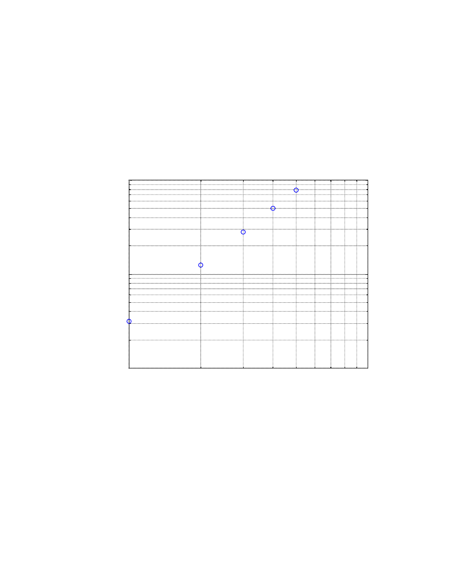
If we prefer a plot of our data, we use the line commands for plotting and labeling as
statements in our code. And, because circle area is a power function of radius, we use the
loglog command to generate a log-log plot of area versus radius.

%

This program will generate a log-log plot

%

of area versus radius for circles of radii

%

from 1 to 5 inches.

for R = 1.0:1.0:5.0

AREA = pi * R^2;
loglog(R,AREA,'o')
hold on
end

xlabel('Circle Radius R, inches')
ylabel('Circle Area A, square inches')
grid
title('THE INFLUENCE OF CIRCLE RADIUS ON CIRCLE AREA')

Division of Engineering Fundamentals , Copyright 1999 by J.C. Malzahn Kampe 20 / 21
Virginia Polytechnic Institute & State University EF1015 Revised Fall 2000
_____________________________________________________

The figure shown below was generated upon execution of the preceding code. The only
editing done in MATLAB’s figure window was moving the figure title to its proper place
below the x-axis. It should be noted that these values are not experimental, and, strictly
speaking, should not be evident as points on the plot. However, in the code above, we
asked for point-by-point plotting because the plot command was inside the loop; this
prevents MATLAB from using a line to plot the values.

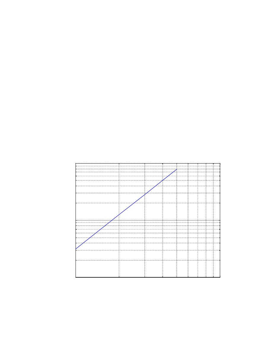
If we want a line instead of points for this plot, we can build two vectors inside the loop
to store our radius and area values, and then have a plot command subsequent to the loop.
This is actually a more efficient way of programming because the plot command is only
executed once instead of five times. It also has the advantage of saving each value of
radius and area that are generated within the loop. See the example code and output
figure found on the following page.

1 0

0

1 0

1

1 0

0

1 0

1

1 0

2

C i r c l e R a d i u s R , i n c h e s

Circle Area A, square inches

T H E I N F L U E N C E O F C I R C L E R A D I U S O N C I R C L E A R E A

Division of Engineering Fundamentals , Copyright 1999 by J.C. Malzahn Kampe 21 / 21
Virginia Polytechnic Institute & State University EF1015 Revised Fall 2000
_____________________________________________________

%

This program will generate a log-log plot

%

of area versus radius for circles of radii

%

from 1 to 5 inches.

N = 0;

for R = 1.0:1.0:5.0
N = N + 1;
AREA(N) = pi * R^2;
RADIUS(N) = R;
end

loglog(RADIUS,AREA,'-')
hold on
xlabel('Circle Radius R, inches')
ylabel('Circle Area A, square inches')

grid
title('THE INFLUENCE OF CIRCLE RADIUS ON CIRCLE AREA')

1 0

0

1 0

1

1 0

0

1 0

1

1 0

2

C i r c l e R a d i u s R , i n c h e s

Circle Area A, square inches

T H E I N F L U E N C E O F C I R C L E R A D I U S O N C I R C L E A R E A