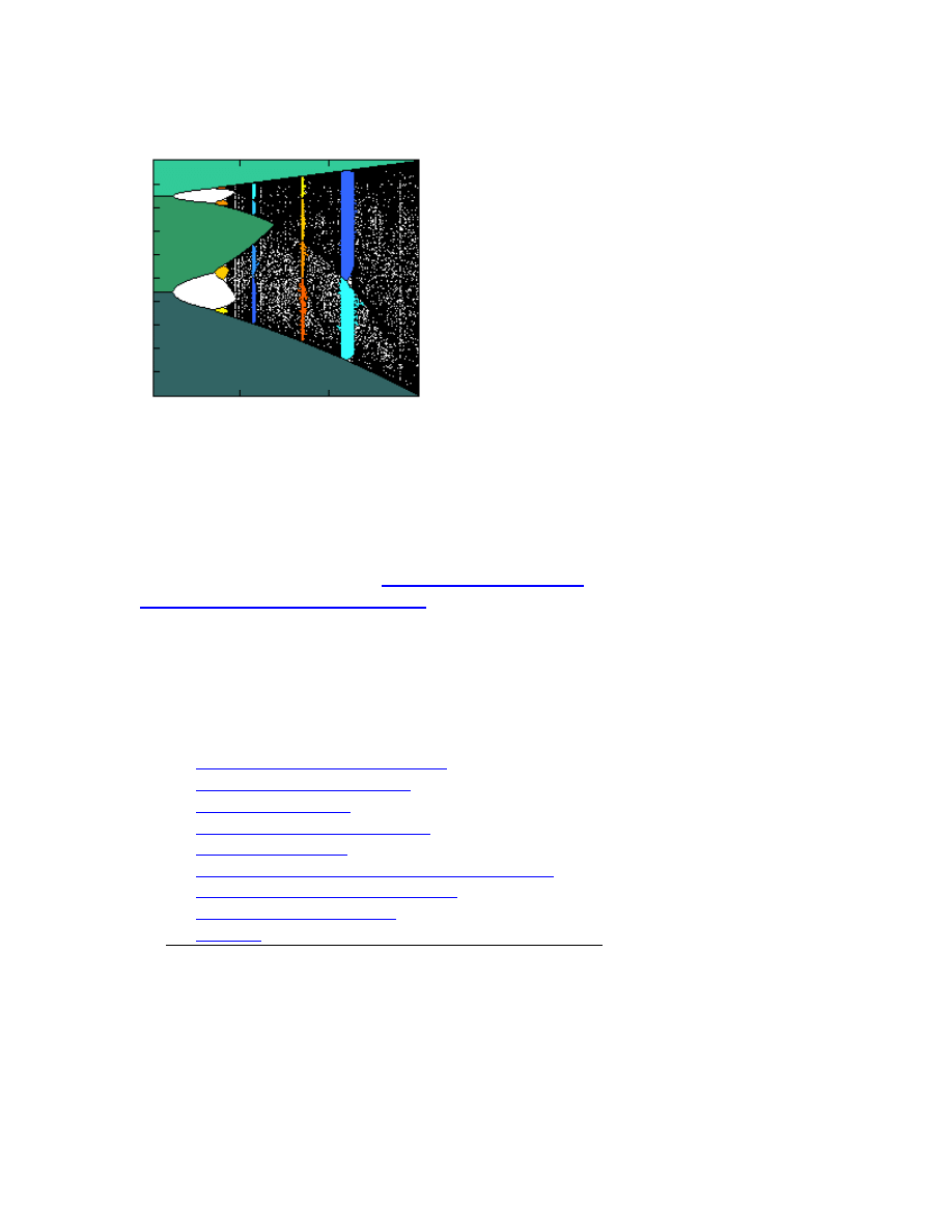
Basic
Concepts
in
Nonlinear
Dynamics
and Chaos

"Out of confusion comes chaos.

Out of chaos comes confusion and fear.

Then comes lunch."

A Workshop

presented at the

Society for Chaos Theory

in Psychology and the Life Sciences

meeting, July 31,1997

at Marquette University, Miwaukee, Wisconsin. © Keith
Clayton

Table of Contents

•

Introduction to Dynamic Systems

•

Nonlinear Dynamic Systems

•

Bifurcation Diagram

•

Sensitivity to Initial Conditions

•

Symptoms of Chaos

•

Two- and Three-dimensional Dynamic Systems

•

Fractals and the Fractal Dimension

•

Nonlinear Statistical Tools

•

Glossary

Introduction to Dynamic Systems

What is a dynamic system?

A dynamic system is a set of functions (rules, equations) that
specify how variables change over time.

First example

...

Alice's height diminishes by half every minute...

Second example

...

x

new

= x

old

+ y

old

y

new

= x

old

The second example illustrates a system with two variables,
x and y. Variable x is changed by taking its old value and
adding the current value of y. And y is changed by becoming
x's old value. Silly system? Perhaps. We're just showing that
a dynamic system is any well-specified set of rules.

Here are some important Distinctions:

•

variables (dimensions) vs. parameters

•

discrete vs. continuous variables

•

stochastic vs. deterministic dynamic systems

How they differ:

•

Variables change in time, parameters do not.

•

Discrete variables are restricted to integer values,
continuous variable are not.

•

Stochastic systems are one-to-many; deterministic
systems are one-to-one

This last distinction will be made clearer as we go
along ...

Terms

The current state of a dynamic system is specified by the
current value of its variables, x, y, z, ...
The process of calculating the new state of a discrete system
is called iteration.

To evaluate how a system behaves, we need the functions,
parameter values and initial conditions or starting state.

To illustrate

...Consider a classic learning theory, the alpha

model, which specifies how q

n

, the probability of making an

error on trial n, changed from one trial to the next
q

n+1

= ß q

n

The new error probability is diminished by ß

(which is less than 1, greater than 0). For example, let the the
probability of an error on trial 1 equal to 1, and ß equal .9.
Now we can calculate the dynamics by iterating the function,

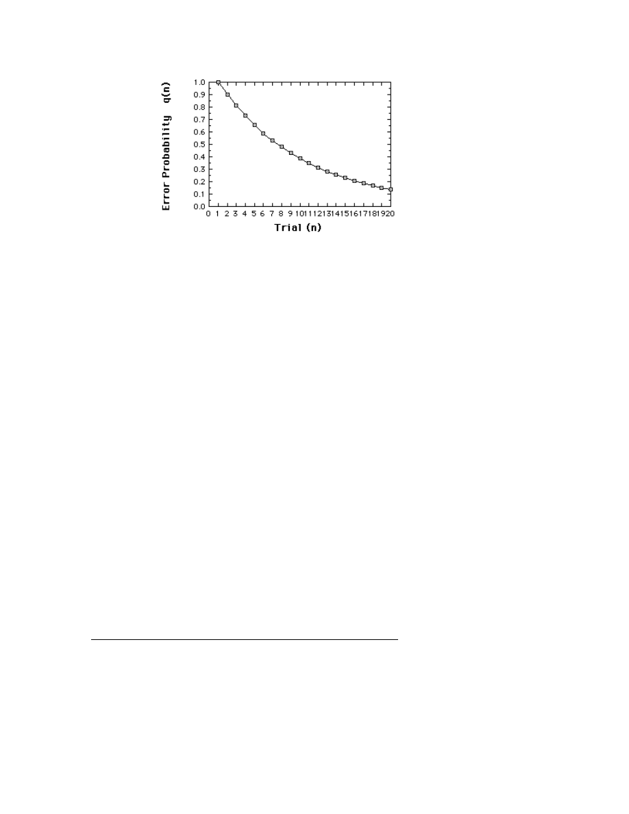
and plot the
results.

q

1

= 1

q

2

= ßq

1

=

(.9)(1) = .9

q

3

= (.9)q

2

=

(.9)(.9) = .81

etc. ...

Error probabilities for the alpha model, assuming q

1

=1, ß

=.9. This "learning curve" is referred to as a time series.

So far, we have some new ideas, but much is old ...

What's not new

Dynamic Systems
Certainly the idea that systems change in time is not new.
Nor is the idea that the changes are probabilistic.

What's new

Deterministic nonlinear dynamic systems.

As we will see, these systems give us:

•

A new meaning to the term unpredictable.

•

A different attitude toward the concept of variability.

•

Some new tools for exploring time series data and for
modeling such behavior.

•

And, some argue, a new paradigm.

This last point is not pursued here.

Nonlinear Dynamic Systems

Nonlinear functions

What's a linear function?

Well, gee Mikey, it's one that can be written in the form of a
straight line. Remember the formula ...
y = mx + b
where m is the slope and b is the y-intercept?

What's a nonlinear function?

What makes a dynamic system nonlinear ....
is whether the function specifying the change is nonlinear.
Not whether its behavior is nonlinear.
And

y is a nonlinear function of x if

x is multiplied by

another (non-constant) variable, or multiplied by itself (i. e.,
raised to some power).

We illustrate nonlinear systems using ...

Logistic Difference Equation

... a model often used to introduce chaos. The Logistic
Difference Equation, or Logistic Map, though simple,
displays the major chaotic concepts.

Growth model

We start, generally, with a model of growth.

x

new

= r x

old

We prefer to write this in terms of n:

x

n+1

= r x

n

.

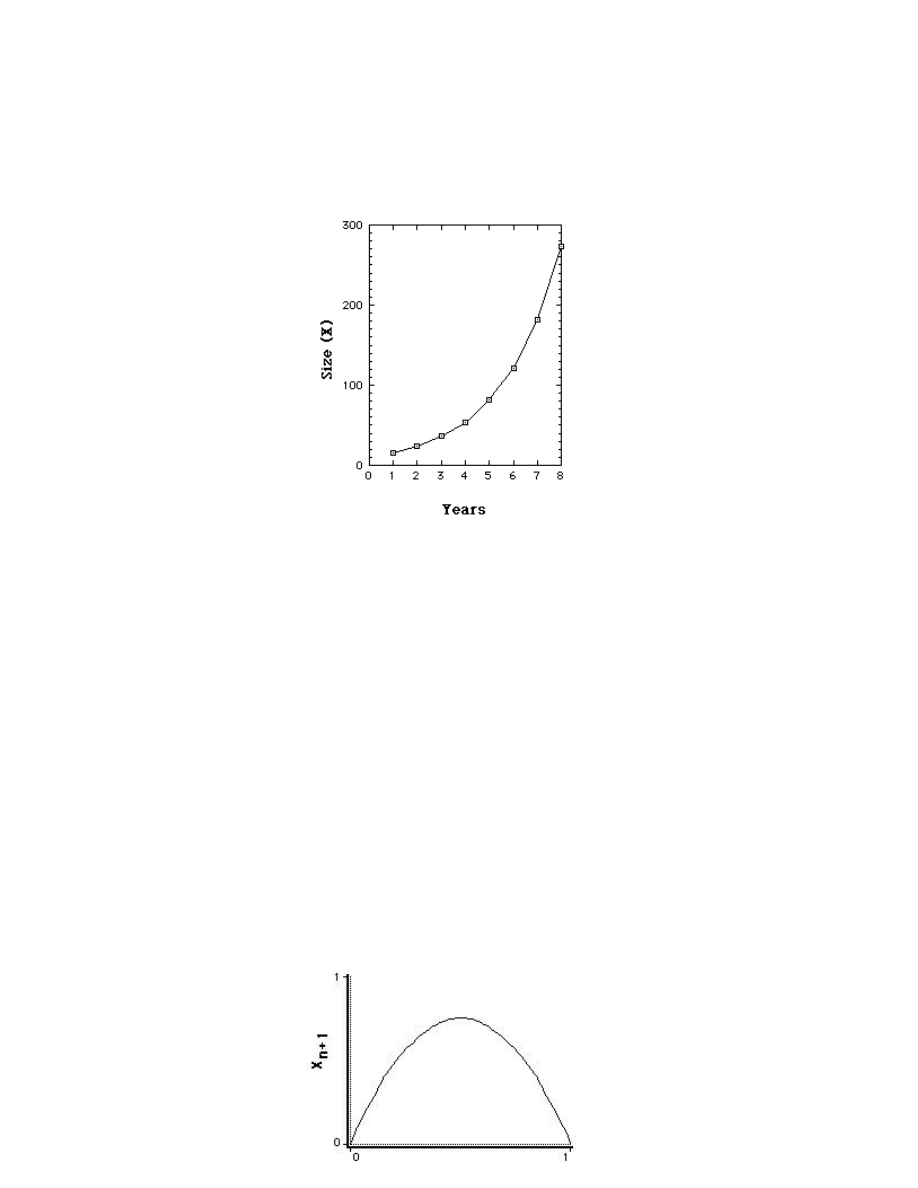
This says x changes from one time period, n, to the next,
n+1, according to r. If r is larger than one, x gets larger with
successive iterations If r is less than one, x diminishes. (In
the "Alice" example at the beginning, r is .5).
Let's set r to be larger than one...

We start, year 1 (n=1),
with a population of 16
[x

1

=16], and since

r=1.5, each year x is
increased by 50%. So
years 2, 3, 4, 5, ... have
magnitudes 24, 36, 54,
...
Our population is
growing exponentially.
By year 25 we have
over a quarter million.

Iterations of Growth model with r = 1.5

So far, notice, we have a linear model that produces
unlimited growth.

Limited Growth model - Logistic Map.

The Logistic Map prevents unlimited growth by inhibiting
growth whenever it achieves a high level. This is achieved
with an additional term, [1 - x

n

].

The growth measure (x) is also rescaled so that the maximum
value x can achieve is transformed to 1. (So if the maximum
size is 25 million, say, x is expressed as a proportion of that
maximum.)
Our new model is

x

n+1

= r x

n

[1 - x

n

]

[r between 0 and 4.]
The [1-x

n

] term serves to inhibit growth because as x

approaches 1, [1-x

n

]

approaches 0.

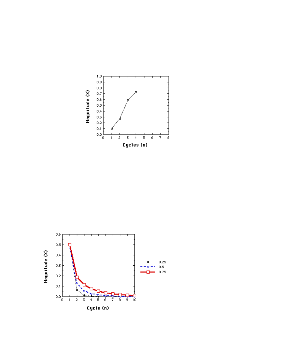
Plotting x

n+1

vs. x

n

, we see we have a nonlinear relation.

Limited growth (Verhulst) model. X

n+1

vs. x

n

, r = 3.

We have to iterate this function to see how it will behave ...
Suppose r=3,
and x

1

=.1

x

2

= rx

1

[1-x

1

] =

3(.1)(.9) = .27

x

3

= r x

2

[1-x

2

]=

3(.27)(.73) =
.591

x

4

= r x

3

[1-

3

]=

3(.591)(.409) =
.725

Behavior of the Logistic map for r = 3, x

1

= .1, iterated to

give x

2

, x

3

, and x

4

It turns out that the logistic map is a very different animal,
depending on its control parameter r. To see this, we next
examine the time series produced at different values of r,
starting near 0 and ending at r=4. Along the way we see very
different results, revealing and introducing major features of
a chaotic system.

When r is less than 1

Behavior of the Logistic map for r=.25, .50, and .75. In all
cases x

1

=.5.

The same fates awaits any starting value. So long as r is less
than 1, x goes toward 0. This illustrates a one-point
attractor.

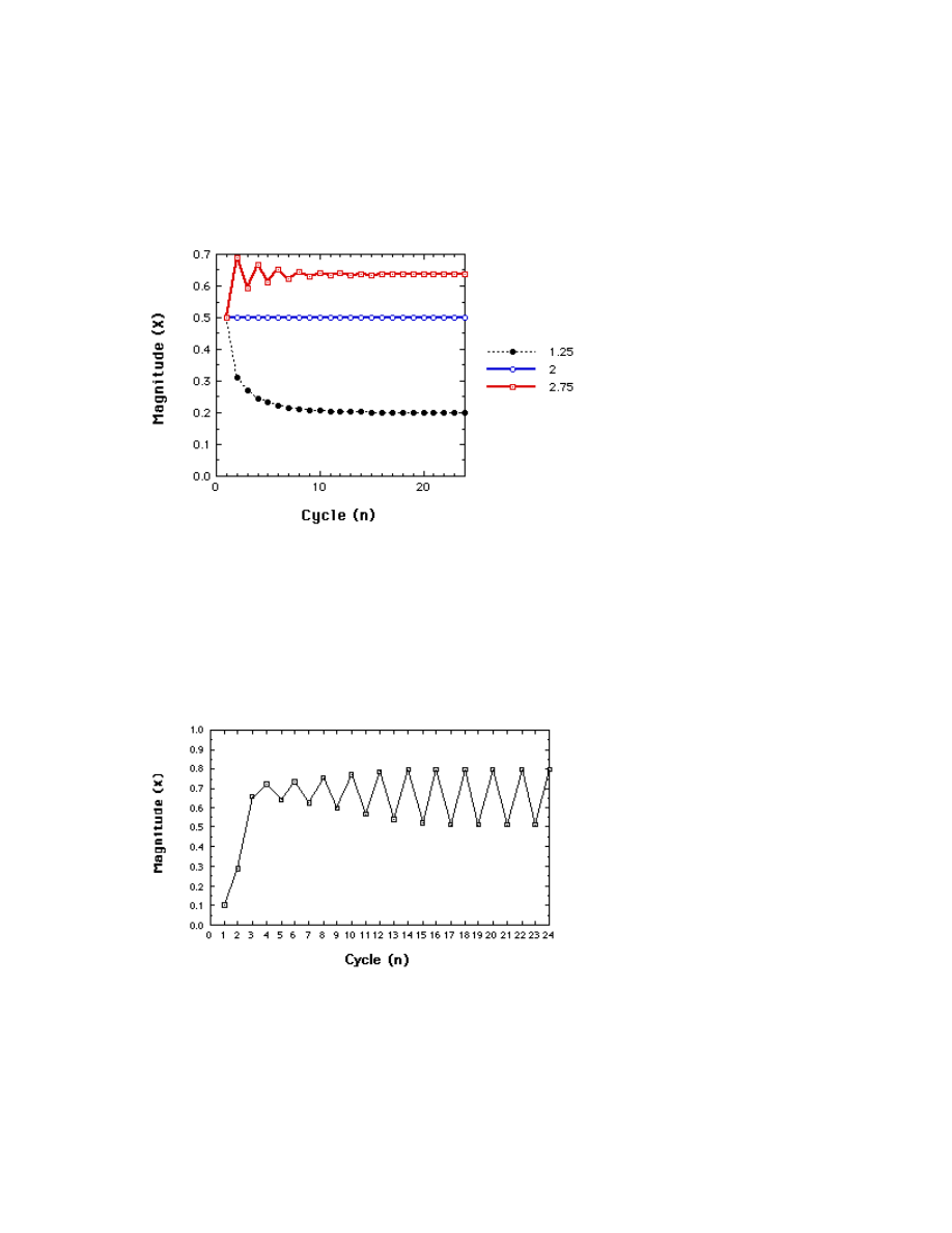
When r is between 1 and 3

Behavior of the Logistic map for r=1.25, 2.00, and 2.75. In
all cases x

1

=.5.

Now, regardless, of the starting value, we have non-zero one-
point attractors.

When r is larger than 3

Behavior of the Logistic map for r=3.2.

Moving just beyond r=3, the system settles down to
alternating between two points. We have a two-point
attractor. We have illustrated a bifurcation, or period

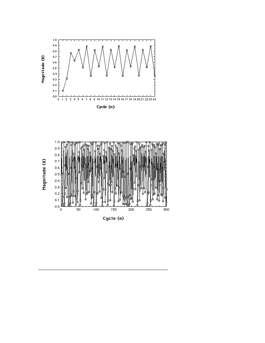
doubling,

Behavior of the Logistic map for r= 3.54. Four-point
attractor

Another bifurcation. The concept: an N-point attractor.

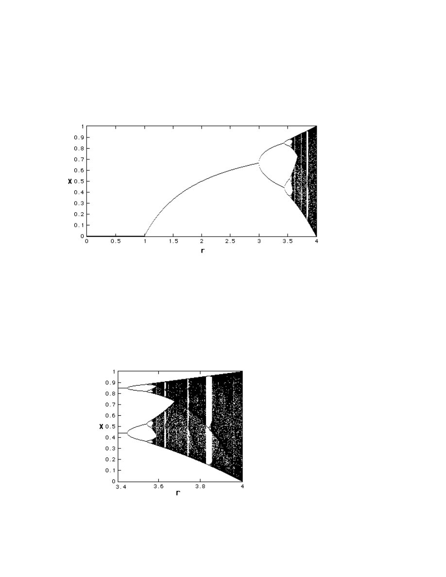
Chaotic behavior of the Logistic map at r= 3.99.

So, what is an attractor? Whatever the system "settles down
to".
Here is a very important concept from nonlinear dynamics: A
system eventually "settles down". But what it settles down to,
its attractor, need not have 'stability'; it can be very 'strange'.

Bifurcation Diagram

So, again, what is a bifurcation? A bifucation is a period-
doubling, a change from an N-point attractor to a 2N-point
attractor, which occurs when the control parameter is

changed.
A Bifurcation Diagram is a visual summary of the
succession of period-doubling produced as r increases. The
next figure shows the bifurcation diagram of the logistic
map, r along the x-axis. For each value of r the system is first
allowed to settle down and then the successive values of x
are plotted for a few hundred iterations.

Bifurcation Diagram r between 0 and 4

We see that for r less than one, all the points are plotted at
zero. Zero is the one point attractor for r less than one. For r
between 1 and 3, we still have one-point attractors, but the
'attracted' value of x increases as r increases, at least to r=3.
Bifurcations occur at r=3, r=3.45, 3.54, 3.564, 3.569
(approximately), etc., until just beyond 3.57, where the
system is chaotic.
However, the system is not chaotic for all values of r greater
than 3.57.
Let's zoom in a bit.

Bifurcation Diagram r between 3.4 and 4

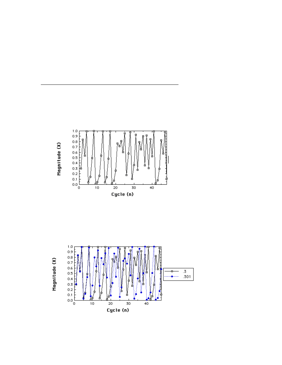
Notice that at several values of r, greater than 3.57, a small
number of x=values are visited. These regions produce the
'white space' in the diagram. Look closely at r=3.83 and you
will see a three-point attractor.
In fact, between 3.57 and 4 there is a rich interleaving of
chaos and order. A small change in r can make a stable
system chaotic, and vice versa.

Sensitivity to initial conditions

Another important feature emerges in the chaotic region ...
To see it, we set r=3.99 and begin at x

1

=.3. The next graph

shows the time series for 48 iterations of the logistic map.

Time series for Logistic map r=3.99, x

1

=.3, 48 iterations.

Now, suppose we alter the starting point a bit. The next
figure compares the time series for x

1

=.3 (in black) with that

for x

1

=.301 (in blue).

Two time series for r=3.99, x

1

=.3 compared to x

1

=.301

The two time series stay close together for about 10
iterations. But after that, they are pretty much on their own.
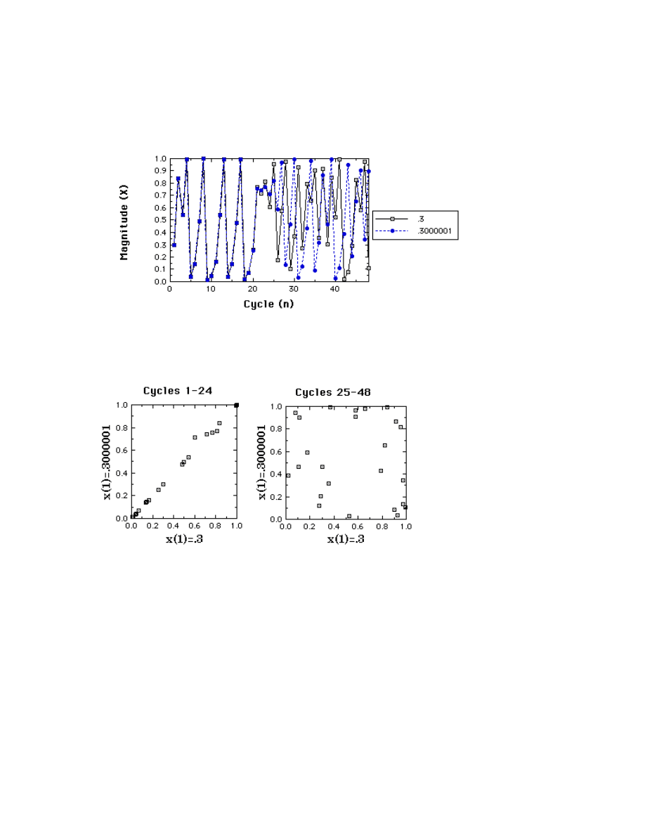
Let's try starting closer together. We next compare starting at
.3 with starting at .3000001...

Two time series for r=3.99, x

1

=.3 compared to x

1

=.3000001

This time they stay close for a longer time, but after 24
iterations they diverge. To see just how independent they
become, the next figure provides scatterplots for the two
series before and after 24 iterations.

Scatterplots of series starting at .3 vs. series starting at

.3000001.

The first 24 cycles on the left, next 24 on the right.

The correlation after 24 iterations (right side), is essentially
zero. Unreliability has replaced reliability.

We have illustrated here one of the symptoms of chaos. A
chaotic system is one for which the distance between two
trajectories from nearby points in its state space diverge over
time. The magnitude of the divergence increases
exponentially in a chaotic system.

So what? Well, it means that a chaotic system, even one
determined by a simple rule, is in principle unpredictable.
Say what? It is unpredictable, "in principle" because in order
to predict its behavior into the future we must know its
currrent value precisely. We have here an example where a
slight difference, in the sixth decimal place, resulted in
prediction failure after 24 iterations. And six decimal places
far exceeds the kind of measuring accuracy we typically
achieve with natural biological systems.

Symptoms of Chaos

We are beginning to sharpen our definition of a chaotic
system. First of all, it is a deterministic system. If we observe
behavior that we suspect to be the product of a chaotic
system, it will also be

difficult to distinguish from random behavior
sensitive to initial conditions

Note well: Neither of these symptoms, on their own, are
sufficient to identify chaos.

Note on technical vs. metaphorical
uses of terms:

Students of chaotic systems have begun to use the (originally
mathematical) terms in a "metaphorical" way. For example,
'bifurcation', defined here as a period doubling has come to
be used to refer to any qualititave change. Even the term
'chaos', has become synomous, for some, with 'overwhelming
anxiety'.

Metaphors enrich our understanding, and have helped extend
nonlinear thinking into new areas. On the other hand, it is
important that we are aware of the technical/metaphorical
difference.

Two- and Three-Dimension Systems

First we practice the distinction between variables
(dimensions) and parameters

Consider again the Logistic map

x

n+1

= r x

n

[1- x

n

]

Multiply the right side out

x

n+1

= r x

n

- r x

n

2

,

and replace the two r's with separate parameters, a and b,

x

n+1

= a x

n

- b x

n

2

.

Now, separate parameters, a and b, govern growth and
suppression, but we still have only one variable, x.

When we have a system with two or more variables,

•

its current state is the current values of its variables,
and is

•

treated as a point in phase (state) space, and

•

we refer to its trajectory or orbit in time.

Predator-prey system

This is a two-dimensional dynamic system in which two
variables grow, but one grows at the expense of the other.
The number of predators is represented by y, the number of
prey by x.

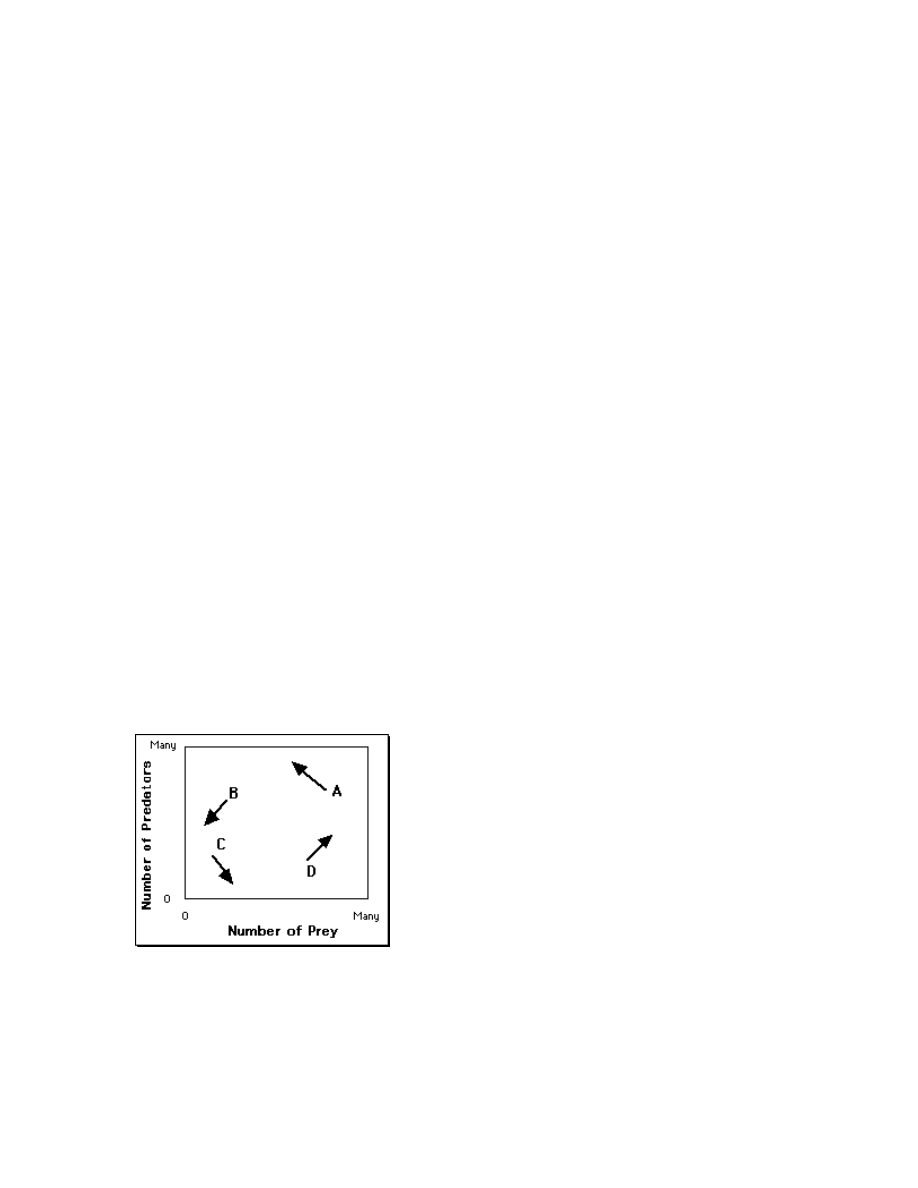
We plot next the phase space of the system, which is a two-

dimension plot of the
possible states of the
system.

A = Too many predators.

B = Too few prey.

C = Few predator and

prey; prey can grow.

D= Few predators, ample

prey.

The phase-space of the predator-prey system.

Four states are shown. At Point A there are a large number
of predators and a large number of prey. Drawn from point A
is an arrow, or vector, showing how the system would

change from that point. Many prey would be eaten, to the
benefit of the predator. The arrow from point A, therefore,
points in the direction of a smaller value of x and a larger
value of y.

At Point B there are many predators but few prey. The
vector shows that both decrease; the predators because there
are too few prey, the prey because the number of predators is
still to the prey's disadvantage. At Point C, since there are a
small number of predators the number of prey can increase,
but there are still too few prey to sustain the predator
population. Finally, at point D, having many prey is
advantageous to the predators, but the number of prey is still
too small to inhibit prey growth, so their numbers increase.
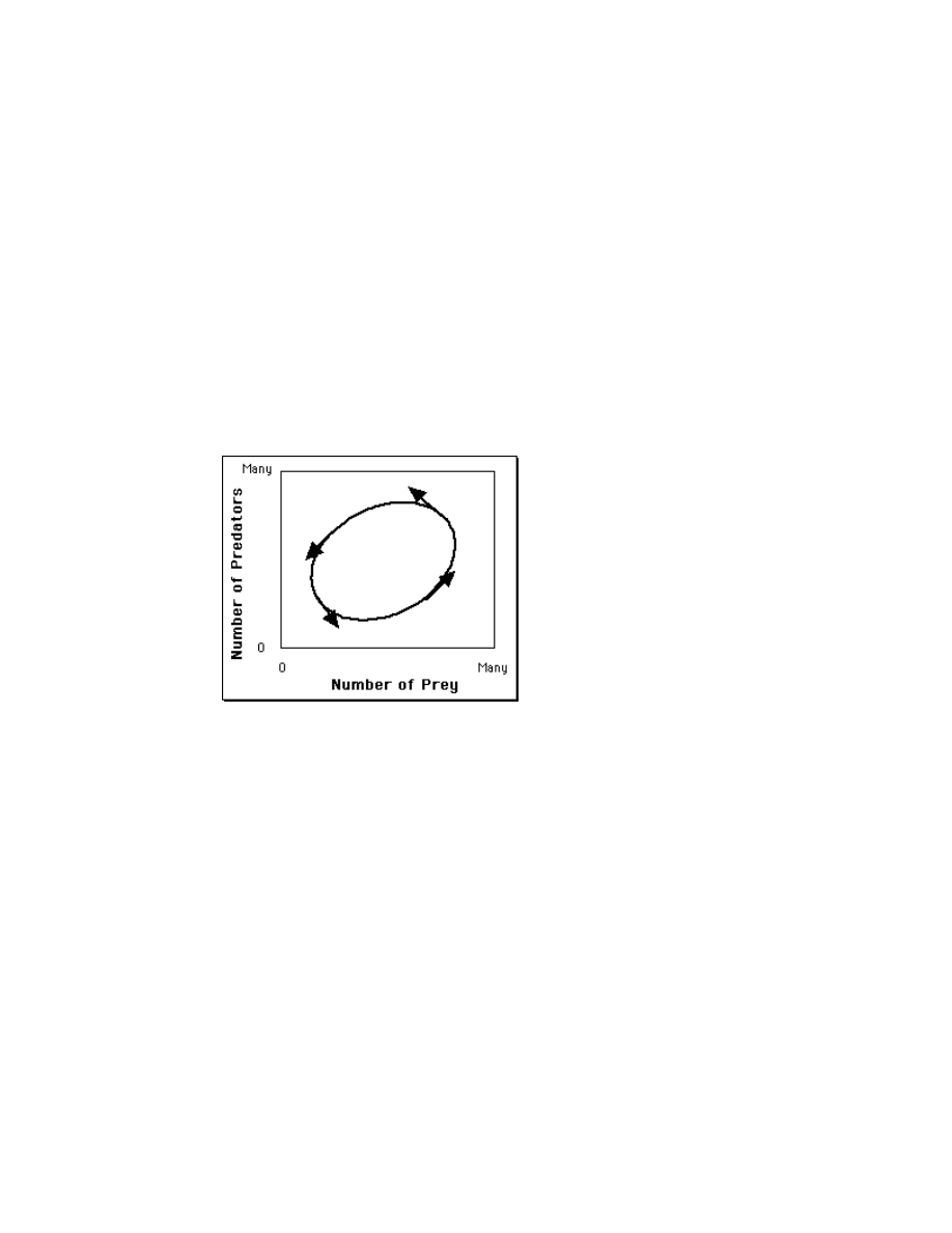
The full trajectory (somewhat idealized) is shown next.

The phase-space of the predator-prey system.

An attractor that forms a loop like this is called a limit cycle.
However, in this case the system doeasn't start outside the
loop and move into it as a final attractor. In this system any
starting state is already in the final loop. This is shown in the
next figure, which shows loops from four different starting
states.

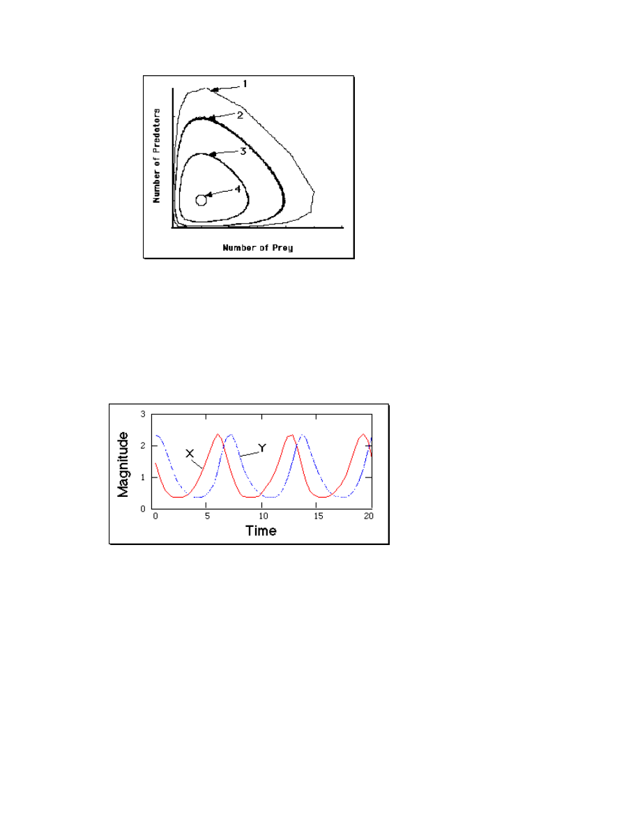
Phase-portrait of the predator-prey system, showing the
influence of starting state.

Points 1-4 start with about the same number of prey but with
different numbers of predators.

Let's look at this system over time, that is, as two time
series.

The time series of the predator-prey system.

This figures shows how the two variables oscillate, out of
phase.

Continuous Functions and Differential Equations

•

Changes in discrete variables are expressed with
difference equations, such as the logistic map.

•

Changes in continuous variables are expressed with
differential equations

For example, the Predator-prey system is typically presented
as a set of two differential equations:

dx/dt = (a-by)x
dy/dt = (cx-d)y

Types of two-dimensional interactions

Other types of two-dimensional interactions are possible, as
nicely categorized by van Geert (1991).

•

mutually supportive - the larger one gets, the faster
the other grows

•

mutually competitive - each negatively affects the
other

•

supportive-competitive - as in Predator-prey

The Buckling column system

Abraham, Abraham, & Shaw (1990) used the Buckling
Column system to discuss psychological phenomena that
exhibit oscillations (for example, mood swings, states of
consciousness, attitude changes). The model is a single,
flexible, column that supports a mass within a horizontally
constrained space. If the mass of the object is sufficiently
heavy, the column will "give", or buckle. There are two
dimensions, x representing the sideways displacement of the
column, and y the velocity of its movement.

Shown next are two situations, differing in the magnitude of
the mass.

The buckling column model (Abraham, Abraham, & Shaw,

1990).

The mass on the left is larger than the mass on the right.

What are the dynamics? The column is elastic, so an initial
give is followed by a springy return and bouncing
(oscillations). If there is resistance (friction), the bouncing
will diminish and the mass will come to rest. The equations
are given for completeness only:
dx/dt = y
dy/dt = (1 - m)(ax

3

+ b + cy)

The parameters m and c represent mass and friction
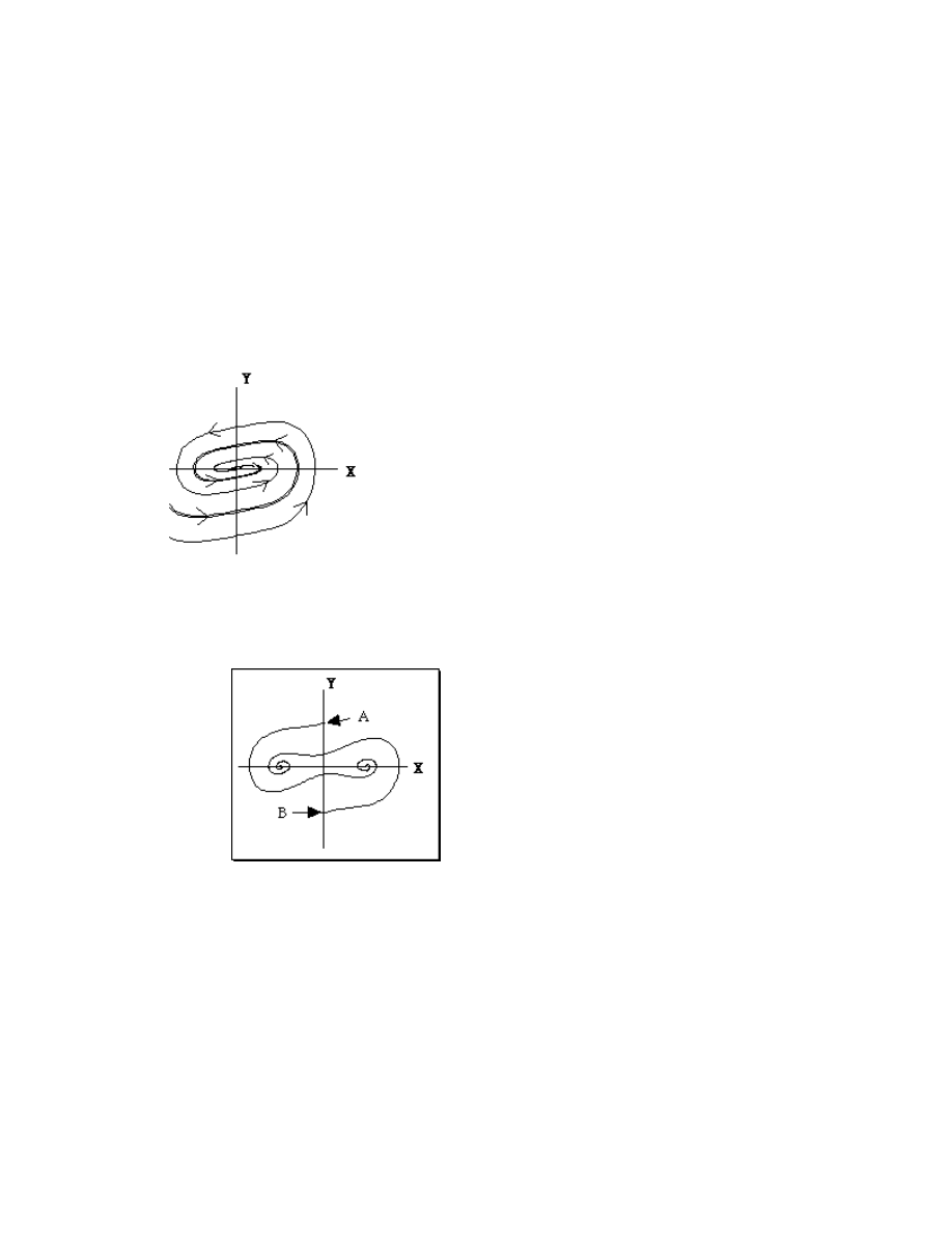
respectively. If there is friction (c>0), and mass is small, the
column eventually returns to the upright position (x=0, y=0),
illustrated next with two trajectories.

Phase portrait of the buckling column model.

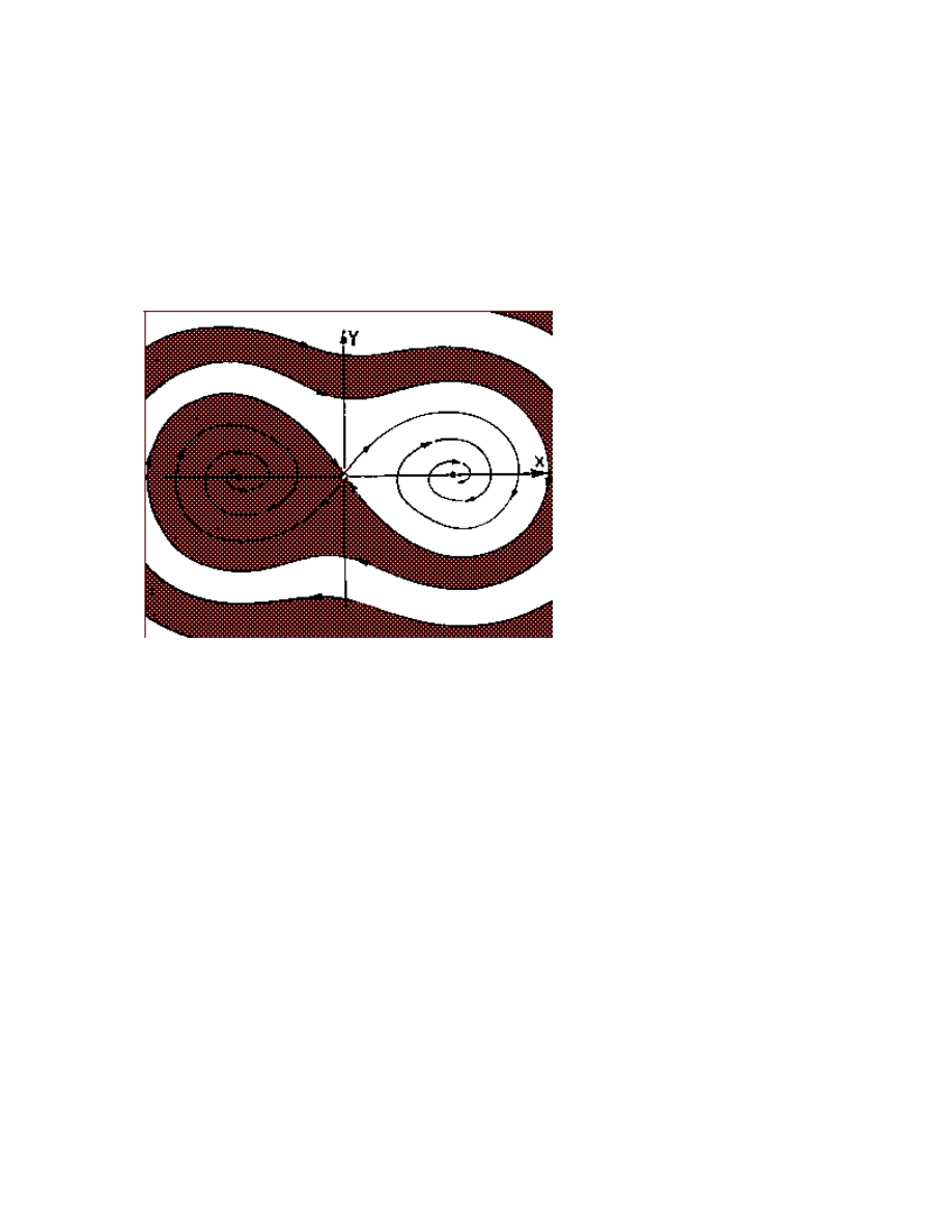
With a heavy mass, the column comes to rest in one of two
positions (two-point attractor), again illustrated with two

trajectories.

Phase portrait of the buckling column model.

Starting at point A, the system comes to rest buckled slightly
to the right, starting at B ends up buckled to the left. Now we
can introduce another major concept...

Basins of attraction

With sufficient mass, the buckling column can end up in one
of two states, buckled to the left or to the right. What

determines which is its fate? For a given set of parameter
values, the fate is determined entirely by where it starts, the
initial values of x and y. In fact, each point in phase space
can be classified according to its attractor. The set of points
associated with a given attractor is called that attractors'
basin of attraction. For the two-point attractor illustrated
here, there are two basins of attraction. These are shown in
the next figure, which has the phase space shaded according
to attractor.

The basins of attraction for the buckling column system.
Reproduced from Abraham et al (1990).

The basin of attraction for the positive attractor (the one on
the right) are shaded. The basin of attraction for the other
attractor is unshaded in the figure. The term seperatrix is
used to refer to the boundary between basins of attraction.

Questions to ponder

Is the buckling column system a chaotic system? Why (not)?

Three-dimensional Dynamic Systems

The Lorenz System

Lorenz's model of atmospheric dynamics is a classic in the
chaos literature. The model nicely illustrates a three-
dimensional system.

dx/dt = a(y-x)
dy/dt = x(b-z) - y
dz/dt = xy-cz

There are three variables reflecting temperature differences
and air movement, but the details are irrelevant to us. We are
interested in the trajectories of the system in its phase space
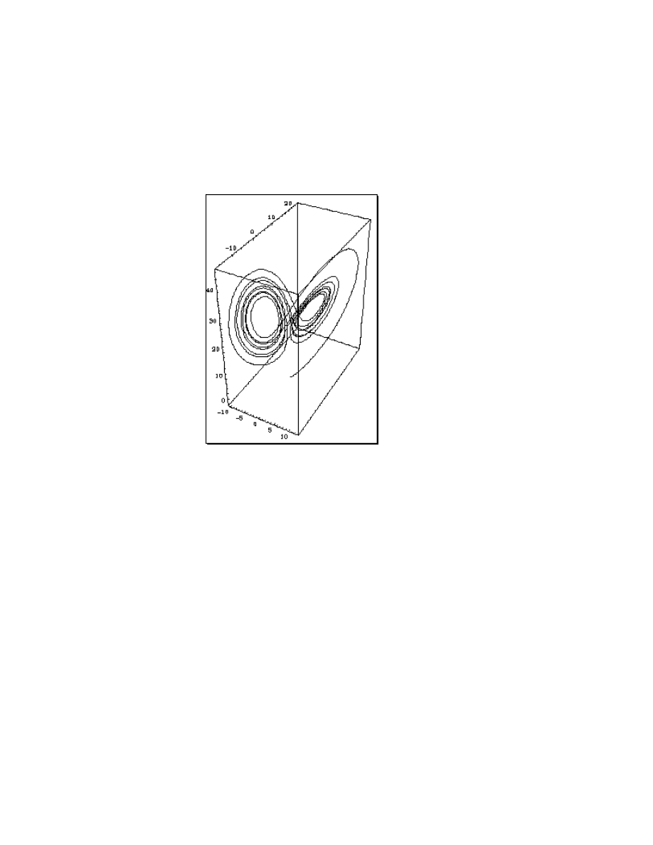
for a=10, b=28, c=8/3. Here we plot part of a trajectory

starting from (5,5,5).

The Lorenz system. Only a portion of one trajectory is
shown.

Although the figure suggests that a trajectory may intersect
with earlier passes, in fact it never does. Although not
demonstrated here, the Lorenz system shows sensitivity to
initial conditions. This is chaos, the first strange attractor,
and it has become the icon for chaos.

Beasts in Phase space - Limit Points

There are three kinds of limit points.

•

Attractors - where the system 'settles down' to.

•

Repellors - a point the system moves away from.

•

Saddle points - attractor from some regions, repellor
to others.

Examples

•

Attractors - we've seen many

•

Repellors - the value 0 in the Logistic Map

•

Saddle points - the point (0,0) in the Buckling
Column

Fractals and the Fractal Dimension

Mandelbrot and Nature

"Clouds are not spheres, mountains are not cones,
coastlines are not circles, and bark is not smooth, nor
does lightning travel in a straight line."(Mandelbrot,
1983).

The Concept of Dimension

So far we have used "dimension" in two senses:

•

The three dimensions of Euclidean space (D=1,2,3)

•

The number of variables in a dynamic system

Fractals, which are irregular geometric objects, require a
third meaning:

The Hausdorff Dimension

If we take an object residing in Euclidean dimension D and
reduce its linear size by 1/r in each spatial direction, its
measure (length, area, or volume) would increase to N=r

D

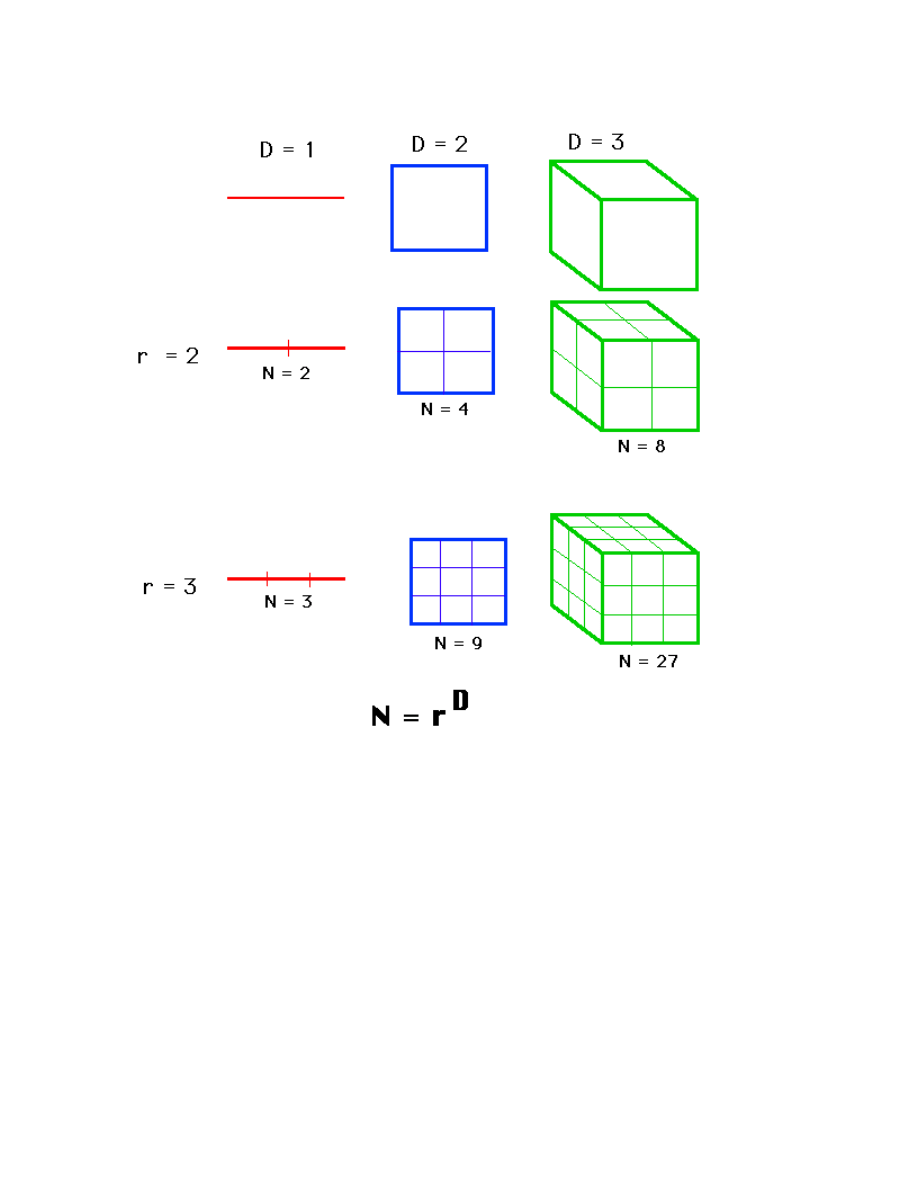
times the original. This is pictured in the next figure.

We consider N=r

D

, take the log of both sides, and get log(N)

= D log(r). If we solve for D. D = log(N)/log(r) The point:
examined this way, D need not be an integer, as it is in
Euclidean geometry. It could be a fraction, as it is in fractal
geometry. This generalized treatment of dimension is named
after the German mathematician, Felix Hausdorff. It has
proved useful for describing natural objects and for
evaluating trajectories of dynamic systems.

The length of a coastline

Mandelbrot began his treatise on fractal geometry by
considering the question: "How long is the coast of Britain?"
The coastline is irregular, so a measure with a straight ruler,
as in the next figure, provides an estimate. The estimated

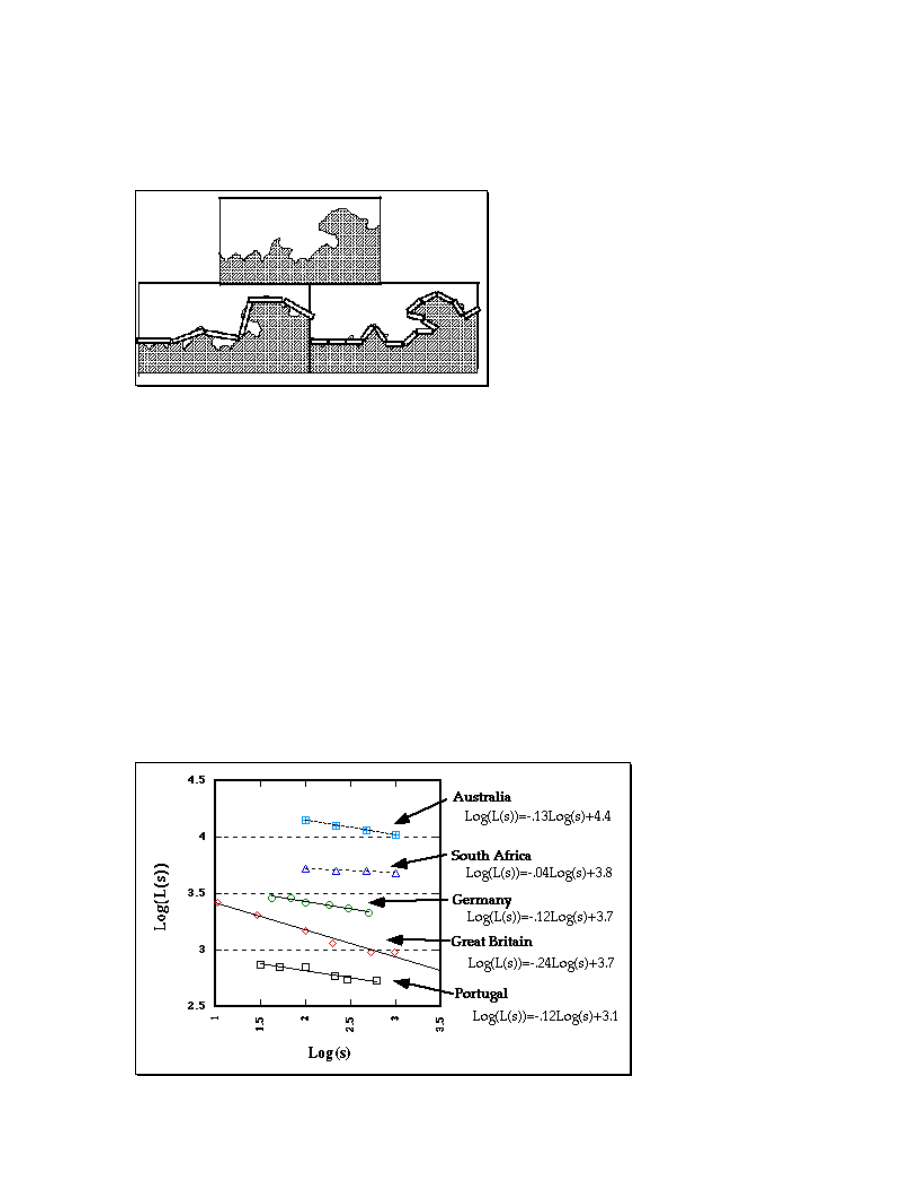
length, L, equals the length of the ruler, s, multiplied by the
N, the number of such rulers needed to cover the measured
object. In the next figure we measure a part of the coastline
twice, the ruler on the right is half that used on the left.

Measuring the length of a coastline using rulers of varying
lengths.

But the estimate on the right is longer. If the the scale on the
left is one, we have six units, but halving the unit gives us 15
rulers (L=7.5), not 12 (L=6). If we halved the scale again, we
would get a similar result, a longer estimate of L. In general,
as the ruler gets diminishingly small, the length gets
infinitely large. The concept of length, begins to make little
sense.

The "Richardson Effect"

Lewis Fry Richardson first noted the regularity between the
length of national boundaries and scale size. As shown next,
the relation between length estimate and length of scale is
linear on a log-log plot.

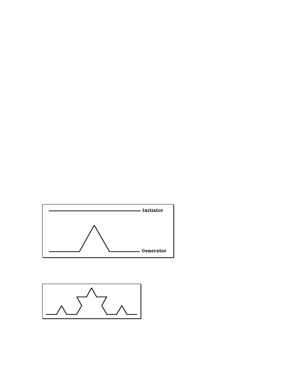
The Richardson Effect.

Mandelbrot assigned the term (1-D) to the slope, so the
functions are:
log[L(s)] = (1-D)log(s) + b where D is the Fractal
Dimension.
For Great Britain, 1 - D = -.24, approximately. D = 1-(-.24) =
1.24, a fractional value.The coastline of South Africa is very
smooth, virtually an arc of a circle. The slope estimated
above is very near zero. D = 1-0 = 1. This makes sense
because the coastline is very nearly a regular Euclidean
object, a line, which has dimensionality of one. In general,
the "rougher' the line, the steeper the slope, the larger the
fractal dimension.

Examples of geometric objects with non-integer
dimensions

Koch Curve

We begin with a straight line of length 1, called the initiator.
We then remove the middle third of the line, and replace it
with two lines that each have the same length (1/3) as the
remaining lines on each side. This new form is called the
generator, because it specifies a rule that is used to generate
a new form.

The Initiator and Generator for constructing the Koch
Curve.

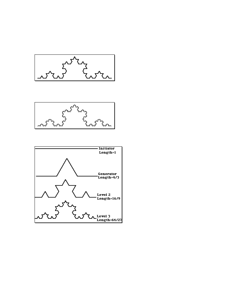
The rule says to take each line and replace it with four lines,
each one-third the length of the original.

Level 2 in the construction of the Koch Curve.

Level 3 in the construction of the Koch Curve.

We do this iteratively ... without end.

The Koch Curve.

What is the length of the Koch curve?

The length of the curve increases with each iteration. It has
infinite length. But if we treat the Koch curve as we did the
coastline, ...

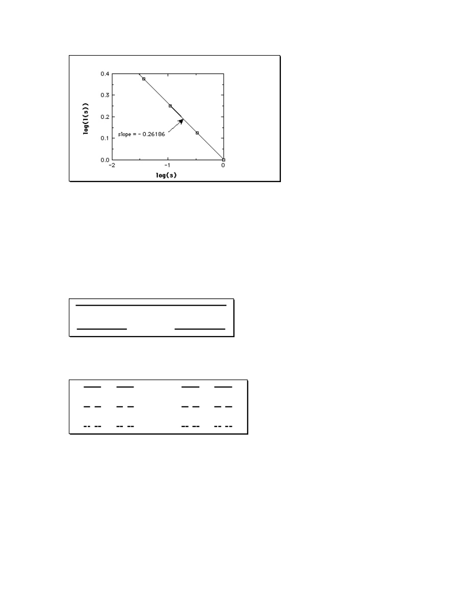
The relation between log(L(s)) and log(s) for the Koch curve
...

we find its fractal dimension to be 1.26. The same result
obtained from D = log(N)/log(r) D = log(4)/log(3) = 1.26.

Cantor Dust

Iteratively removing the middle third of an initiating straight
line, as in the Koch curve, ...

Initiator and Generator for constructing Cantor Dust. ...

this time without replacing the gap...

Levels 2, 3, and 4 in the construction of Cantor Dust.

Calculating the dimension ... D = log(N)/log(r) D =
log(2)/log(3) = .63 We have an object with dimensionality
less than one, between a point (dimensionality of zero and a
line (dimensionality 1).

Sierpinski Triangle

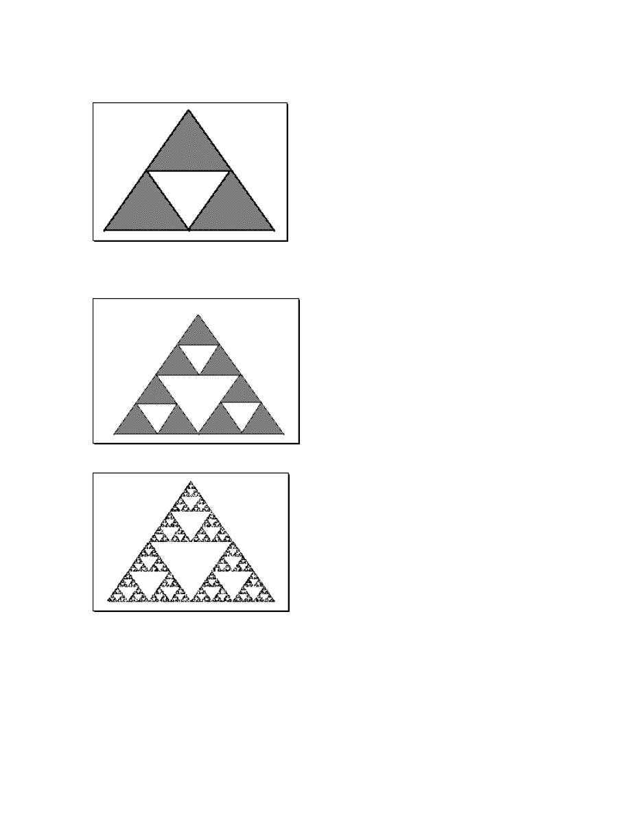
We start with an equilateral triangle, connect the mid-points
of the three sides and remove the resulting inner triangle.

Constructing the Sierpinski Triangle.

Iterating the first step.

Constructing the Sierpinski Triangle.

The Sierpinski Triangle.

Calculating the dimension... D = log(N)/log(r) =
log(3)/log(2) = 1.585. This time we get a value between 1
and 2.

The dimensionality of a strange attractor

1. The trajectory of a strange attractor cannot intersect

with itself. (Why?)

2. Nearby trajectories diverge exponentially. (Why?)
3. But the attractor is bounded to the phase space.
4. The trajectory does not fill the phase space.

A strange attractor is a fractal, and its fractal dimension is
less than the dimensions of its phase space.

Self-similarity

An important (defining) property of a fractal is self-
similarity, which refers to an infinite nesting of structure on
all scales. Strict self- similarity refers to a characteristic of a
form exhibited when a substructure resembles a
superstructure in the same form.

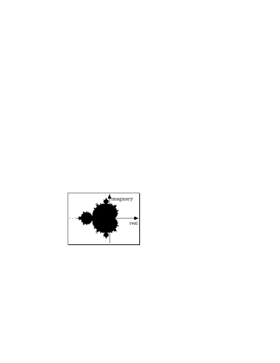
Mandelbrot Set

Found by iterating
z

n+1

= z

n

2

+ c.

where z is a complex number. z

0

=0.

For different values of c, the trajectories either: stay near the
origin, or "escape".
The Mandelbrot set is the set of points that are not in the

Escape Set.

The Mandelbrot set. The points in the set are painted black.

The Escape Set differs in rate of escape, graphically depicted
with different colors or altitudes ...

Constructed using the computer program "The Beauty of

Fractal Lab", by Thomas Eberhardt.

So, what is a fractal?

An irregular geometric object with an infinite nesting of
structure at all scales.

Why do we care about fractals?

•

Natural objects are fractals.

•

Chaotic trajectories (strange attractors) are fractals.

•

Assessing the fractal properties of an observed time
series is informative.

Nonlinear Statistical Tools

A number of statistical techniques have been introduced to
try to evaluate time series data. Their purposes include 1)
attempting to distinguish chaotic time series from random
data ("noise"), 2) assessing the feasibility that the data are the
product of a deterministic system, and 3) assessing the
dimensionality of the data. Here we introduce some concepts
basic to these efforts.

Return Maps

What is a return map?

A plot of x

t

against x

delta t

Why is it plotted?

To evaluate the structure of the measured trajectory.

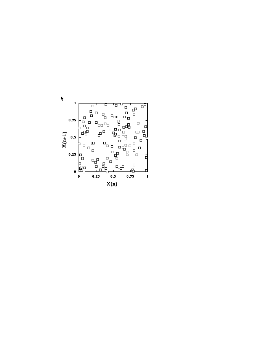
To illustrate, we start with a time series that was generated
by randomly sampling from (0,1) interval. If we plot x

n

against x

n+1

we get ...

Return Map of time series from random Uniform

distribution.

As expected, the points scatter.

Here's a return map from another random time series.
This one sampled from an exponential (positively skewed)
distribution.

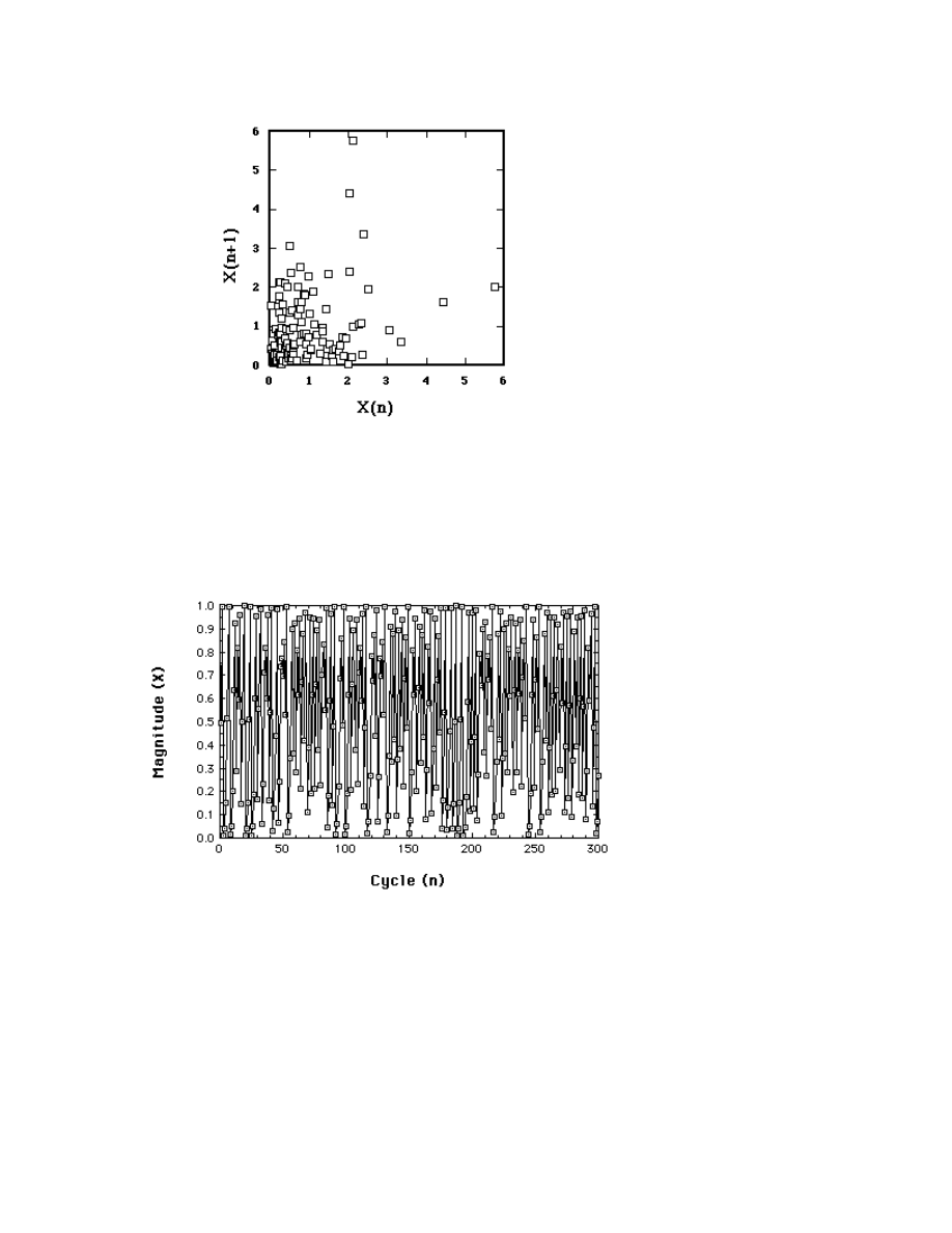
Return Map of time series from exponential distribution.

Here we do not scatter all over. What's the point? You may
have heard that a symptom of chaos is when the return map
is confined to a region of the map. This illustrates how such a
collection can occur, but from a random system.

Now, remember this time series?

A nonrandom Time Series

It's from the Logistic Map in the chaotic region, r=3.99.
What does its Return Map look like?

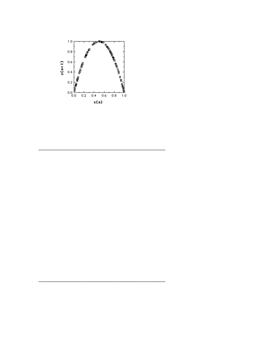
Return Map from Logistic Map, r=3.99

The structure of the generating function is entirely captured.

So, a return map can be very handy, provided the data are
from a one-dimensional system. If the system has more than
two-dimensions, the return map has limited utility.

Embedding dimension

Okay. One more meaning of the term 'dimension'.
It comes from extending the concept of a return map.
Successive n- tuples of data are treated as points in n-space.
The Return Map is an embedding dimension of 2.

Suppose, for example, that the first six data values were
4, 2, 6, 1, 5, 3,
then for an embedding dimension of 3.
P(1)= (4,2,6)
P(2)= (2,6,1)
P(3)= (6,1,5), and so forth.

What's the point?

Contemporary statistical analyses examine the geometric
structure of obtained time series embedded with differing
dimensions.

Types of 'Noise'

An older, linear, tool, for examining time series, is Fourier
analysis, specifically, FFT (Fast Fourier Transform). FFT
transforms the time domain into a frequency domain, and
examines the series for periodicity. The analysis produces a
power spectrum, the degree to which each frequency
contributes to the series. If the series is periodic, then the
resulting power spectrum reveals peak power at the driving
frequency.
Plotting log power versus log frequency,

•

White noise (and many chaotic systems) have zero
slope.

•

Brown noise has slope equal to -2.

•

1/f (Pink) noise has a slope of -1.

1/f noise is interesting because it is ubiquitous in nature, and
it is a sort of temporal fractal. In the way a fractal has self-
similarity in space, 1/f noise has self-similarity in time.
Pink noise is also a major player in the area of complexity,
our next topic.

Glossary

Definitions of several terms are a matter of some dispute.
For a more technical treatment of some of these terms, see
the

faq sheet of the sci.nonlinear newsgroup.

attractor The status that a dynamic system eventually
"settles down to". An attractor is a set of values in the phase
space to which a system migrates over time, or iterations. An
attractor can be a single fixed point, a collection of points
regularly visited, a loop, a complex orbit, or an infinite
number of points. It need not be one- or two-dimensional.
Attractors can have as many dimensions as the number of
variables that influence its system.
basin of attraction A region in phase space associated with
a given attractor. The basin of attraction of an attractor is the
set of all (initial) points that go to that attractor.
bifurcation A qualitative change in the behavior (attractor)
of a dynamic system associated with a change in control
parameter.
bifurcation diagram Visual summary of the succession of
period-doubling produced as a control parameter is changed.
chaos Behavior of a dynamic system that has (a) a very large
(possibly infinite) number of attractors and (b) is sensitive to
initial conditions.
complexity While, chaos is the study of how simple systems

can generate complicated behavior, complexity is the study
of how complicated systems can generate simple behavior.
An example of complexity is the synchronization of
biological systems ranging from fireflies to neurons. (From
the FAQ sheet of the sci.nonlinear newsgroup).
complex system Spatially and/or temporally extended
nonlinear systems characterized by collective properties
associated with the system as a whole--and that are different
from the characteristic behaviors of the constituent
parts.(From the FAQ sheet of the sci.nonlinear newsgroup)
control parameter A parameter in the equations of a
dynamic system. If control parameters are allowed to change,
the dynamic system would also change. Changes beyond
certain values can lead to bifurcations. .
difference equation A function specifying the change in a
variable from one discrete point in time to another.
differential equation A function that specifies the rate of
change in a continuous variable over changes in another
variable (time, in this book).
dimension See embedding dimension, box-counting
dimension, correlation dimension, information dimension,
dimension of a system.
dimensions of a system The set of variables of a system.
dynamic system A set of equations specifying how certain
variables change over time. The equations specify how to
determine (compute) the new values as a function of their
current values and control parameters. The functions, when
explicit, are either difference equations or differential
equations. Dynamic systems may be stochastic or
deterministic. In a stochastic system, new values come from
a probability distribution. In a deterministic system, a single
new value is associated with any current value.
embedding dimension Successive N-tuples of points in a
time series are treated as points in N dimensional space. The
points are said to reside in embedding dimensions of size N,
for N = 1, 2, 3, 4, ... etc.
fractal An irregular shape with self-similarity. It has infinite
detail, and cannot be differentiated. "Wherever chaos,
turbulence, and disorder are found, fractal geometry is at
play" (Briggs and Peat, 1989).
fractal dimension A measure of a geometric object that can
take on fractional values. At first used as a synonym to
Hausdorff dimension, fractal dimension is currently used as a
more general term for a measure of how fast length, area, or
volume increases with decrease in scale. (Peitgen, Jurgens, &
Saupe, 1992a).

Hausdorff dimension A measure of a geometric object that
can take on fractional values. (see fractal dimension).
initial condition the starting point of a dynamic system.
iteration the repeated application of a function, using its
output from one application as its input for the next.
iterative function a function used to calculate the new state
of a dynamic system.
iterative system A system in which one or more functions
are iterated to define the system.
limit cycle An attractor that is periodic in time, that is, that
cycles periodically through an ordered sequence of states.
limit points Points in phase space. There are three kinds:
attractors, repellors, and saddle points. A system moves away
from repellors and towards attractors. A saddle point is both
an attractor and a repellor, it attracts a system in certain
regions, and repels the system to other regions.
linear function The equation of a straight line. A linear
equation is of the form y=mx+b, in which y varies "linearly"
with x. In this equation, m determines the slope of the line
and b reflects the y-intercept, the value y obtains when x
equals zero.
logistic difference equation see logistic map
logistic map x(n+1)= rx(n)[1- x(n)]. A concave-down
parabolic function that (with 0<r
Lorenz attractor A butterfly-shaped strange attractor. It
came from a meteorological model developed by Edward
Lorenz with three equations and three variables. It was one of
the first strange attractors studied.
Lyapunov Number (Liapunov number) The value of an
exponent, a coefficient of time, that reflects the rate of
departure of dynamic orbits. It is a measure of sensitivity to
initial conditions.
nonlinear function One that's not linear! y would be a
nonlinear function of x if x were multiplied by another
variable (non-constant) or by itself (that is, raised to some
power.
nonlinear dynamics The study of dynamic systems whose
functions specifying change are not linear.
orbit (trajectory) A sequence of positions (path) of a system
in its phase space.
period-doubling The change in dynamics in which a N-point
attractor is replaced by a 2N-point attractor.
phase portrait The collection of all trajectories from all
possible starting points in the phase space of a dynamic
system.
phase space (state space) An abstract space used to

represent the behavior of a system. Its dimensions are the
variables of the system. Thus a point in the phase space
defines a potential state of the system. The points actually
achieved by a system depend on its iterative function and
initial condition (starting point).
recursive process For our purposes, "recursive" and
"iterative" are synonyms. Thus recursive processes are
iterative processes, and recursive functions are iterative
functions.
repellors One type of limit point. A point in phase space that
a system moves away from.
return map Plot of a time series values n vs. n+1.
saddle point A point, usually in three-space, that both an
attracts and a repels, attracting in one dimension and
repelling to another.
self-similarity An infinite nesting of structure on all scales.
Strict self- similarity refers to a characteristic of a form
exhibited when a substructure resembles a superstructure in
the same form.
sensitivity to initial conditions A property of chaotic
systems. A dynamic system has sensitivity to initial
conditions when very small differences in starting values
result in very different behavior. If the orbits of nearby
starting points diverge, the system has sensitivity to initial
conditions.
starting state see initial condition
state A point in state space designating the current location
(status) of a dynamic system.
state space (phase space) An abstract space used to
represent the behavior of a system. Its dimensions are the
variables of the system. Thus a point in the phase space
defines a potential state of the system.
strange attractor N-point attractor in which N equals
infinity. Usually (perhaps always) self-similar in form.
time series A set of measures of behavior over time.
Torus An attractor consisting of N independent oscillations.
Plotted in phase space, a 2-oscillation torus resembles a
donut.
trajectory (orbit) A sequence of positions (path) of a system
in its phase space. The path from its starting point (initial
condition) to and within its attractor.
vector A two-valued measure associated with a point in the
phase space of a dynamic system. Its 1) direction shows
where the system is headed from the current point, and its 2)
length indicates velocity.
vector field The set of all vectors in the phase space of a

dynamic system. For a given continuous system, the vector
field is specified by its set of differential equations.