Application of Neural Networks to

Stock Market Prediction

Amol S. Kulkarni



 1996 Amol S. Kulkarni

All rights reserved.

Material in this report may not be reproduced in any form. This material is

made available for learning and may not be used in any manner for any

profit activities without the permission of the author.

1

Introduction

The aim of this project is to predict the future values of the Standard & Poor’s 500 (S&P
500) stock index based on its past values and the past values of some financial indicators.
There have been many attempts at predicting stock market movements, most of them
based on statistical time series models [1]. Most of these attempts have been unsuccessful
due to the complex dynamics of the stock market. The efficient market hypothesis says
that stock prices rapidly adjust to new information by the time the information becomes
public knowledge, so that prediction of stock market movements is impossible [2]. This
hypothesis seems to be correct for static and linear relationships explored traditionally
using multiple regression analysis. However, it is possible that dynamic and non-linear
relationships exist which cannot be modeled by traditional time series analysis methods
[3]. This, is the motivation for application of neural networks to financial time series
analysis.

A huge amount of research is being done on the application of neural networks to stock
markets. Some of the applications include prediction of IBM daily stock prices [4], a
trading system based on prediction of the daily S&P 500 index [5], short term trend
prediction using dual-module networks [6], weekly index prediction [7], monthly index
prediction using radial basis functions [8] etc. Some of these papers use the past values of
the stock index only, as the input to the neural network so as to obtain the future values,
while some use additional fundamental and financial factors as inputs.

This project explores the effect that short and long term interest rates have on the stock
market, in particular on the S&P 500 index. It is well known that an increase in interest
rates tends to lower the stock market and vice versa [9]. The hypothesis is that the current
stock prices indicate the cumulative sum of the present and future worth of any company.
If the interest rates increase, the equivalent future value of a stock in terms of today’s
dollars reduces, causing the stock price to reduce. Financial experts report that the long
term value of a broad based index is affected by interest rates after some unknown delay.
However, the exact effect is unknown and hence, a neural network can be suitably applied
to find this non-linear mapping. The next section is a brief review of some of the similar
work done while section three describes the selection of features from the raw data for
training of the neural network. Test results for different strategies are given in section four
and the last section lists the conclusions from this project.

2. Literature review

The work done in the area of stock market prediction using neural networks can be
classified into two broad categories:

•

Prediction using past stock index values and momentum indicators based on

these values, and

•

Prediction using past stock index values and other fundamental factors such as

interest rates, foreign exchange rates, up and down volumes, bond rate etc.

2

Prediction using past stock values only

This first category is based on the theory that all the information available regarding any
economic indicators is already contained in the time history of the index and future index
values are dependent on data upto the present moment. Some applications of this category
are discussed below.

Dual module neural network

One application [6] uses a dual module neural network, with one module learning the long
term trend of the market and the other module trained to learn the short term rate. The
data used is a 4-tuple of index values, namely the high, low and closing values and trading
volume for each day. By taking moving averages and variances, this set of 4-tuples for all
days are combined into a 16-tuple which is level insensitive and time-invariant. These
extracted features are then used to train the two networks. The long term net uses a
training window spanning the last trading quarter while a 12-day window is used for the
short term module. The authors conclude that the neural network shows a much better
response than multiple linear regression.

Neural sequential associator

In this paper [10], the author uses a feedforward neural network with the last n stock
index values as inputs and the next N-n values as the outputs. This is a N-n step ahead
prediction. Thus, if index for the n

th

day is denoted by X

n

, then, the inputs are X

1

, X

2

, ... X

n

and the outputs are X

n+1

, X

n+2

, ..., X

N

. If such a network is trained, any correlation

between the index values for the n+1 through N

th

day will be neglected. To ensure that

this does not happen, the network is trained with errors between the desired and actual
outputs in addition to the n inputs. These errors will then be (X

n+1

- Y

n+1

) ...., where Y is

the output of the network. As training proceeds this error will tend to zero and these
additional inputs are not required in the testing phase. This work also uses two neural
networks, one to learn the global features and another to learn the local features or small
fluctuations.

Recurrent neural network approach

Kamijo and Tanigawa [11] propose the use of an Elman recurrent net for predicting the
future stock prices using extracted features from past daily high, low and closing stock
prices. The method used tries to extract triangle patterns in stock prices which are seen
graphically by plotting the daily high, low and closing prices. A triangle refers to the
beginning of a sudden stock price rise after which the high and low prices appear and the
price oscillates for some period before the lines converge. The neural network is trained to
recognize such triangle patterns in the stock prices. As such, it is mainly a categorization
approach to recognize whether a pattern is a triangle or not. Such knowledge can be
useful in judging whether a price rise is permanent.

Prediction based on past stock values and other fundamental indicators

The second category of research assumes that other fundamental factors such as present
interest rates, bond rate and foreign exchange rates affect the future stock prices. Since,

3

this is also the focus of the present project, some of these papers are described in greater
detail especially with respect to the feature extraction, wherever such information has been
made available in these publications.

Modular neural network approach

Kimoto et al [12] use several neural networks trained to learn the relationships between
past values of various technical and economic indices for obtaining the expected returns of
the TOPIX. The TOPIX is a weighted average of all stocks listed on the Tokyo Stock
Exchange and is similar to the Dow Jones Industrial Average (DJIA). The technical and
economic indices used are: the vector curve (an indicator of market momentum), turnover,
interest rate, foreign exchange rate and the DJIA value. The desired output of the
networks is a weighted sum, over a few weeks, of the logarithm of the ratio of the TOPIX
at the end of week t, to the TOPIX value at the end of week (t-1).
Thus, r

t

= ln(TOPIX(t)/TOPIX(t-1)) and the desired output is a weighted sum of r

t

for some weeks. The feature extraction is not explained in [12] except for the fact that
some irregularity is removed and logarithm function is used before normalization. The
authors claim that the use of the weighted sum of the outputs of many neural networks
reduces the error, especially since the returns are predicted for a few weeks. A buy/sell
system is setup based on the predicted returns and this system is shown to perform much
better than a buy-hold strategy. However, the teaching data uses future returns, so that
this method cannot be used for actual stock trading. (The authors do mention this as part
of their proposed future work).

One week ahead prediction using feedforward networks

This work [7] uses a simple feedforward neural network trained using past and present
data to predict the value of the FAZ-Index which is the German equivalent of the DJIA.
Input data includes the moving average of past 5 and 10 weeks of the FAZ-Index, a first
order difference of the FAZ-Index and its moving averages, the present bond market index
and its first order difference and the Dollar-Mark exchange rate along with its first order
difference. The value of the FAZ index is predicted for the next week based on this data.
The network is trained using data for the past M weeks and is then tested based on data
for the next L weeks, where M is called the training window and L is called the testing
window. For successive prediction, the windows are moved ahead and the network is
retrained. Three different networks are compared each having a different set of inputs, one
of which has only the last 10 FAZ index values as the input. It is seen that the network fed
with technical indicator data performs better than the one trained only on past index
values. Normalization of training data is done so as to keep the data within 0.1 and 0.9,
however, the normalization method is not given. This approach is particularly suitable to
the aim of this project and is hence, used as the basic method in this project with certain
modifications.

Radial basis function approach

Komo, Chang and Ko [8] use a radial basis function network to predict the future stock
index values based on past data of the index and other technical indicators such as
transaction costs, bond market values and futures prices. The RBF network has two

4

hidden layers, with the first hidden layer being trained using the K-means clustering
algorithm which is thus, an unsupervised learning algorithm. Once an initial solution for
the means and standard deviations of each neuron is found using the clustering algorithm,
a supervised learning algorithm is applied to fine tune the parameters of both the hidden
layers. Gradient descent is used for the supervised learning. No details are given regarding
the inputs used or the feature extraction.

Multi-component trading system using S&P 500 prediction

Obradovic et al [5] use two neural networks, to predict the returns on S&P 500 stock
index. One network is trained using upward trending data while another is trained for
downward trending data. The test data is fed to both the neural networks after filtering. A
complex filtering scheme is used based on traditional direction indicators. The outputs of
the two networks are combined using a high level decision rule base to obtain buy/sell
recommendations. The inputs used are the S&P 500 index return for the past 3 days and
the US Treasury rate lagged 2 and 3 months. The authors report that a simple filtering
scheme gives better results than the more complex scheme using directional indicators.
The average annual rate of return obtained using this approach is close to 15% which is
much higher than the return obtained using a buy-hold strategy. This approach is not used
in this project owing to its complexity.

Some of the literature dealing with stock market prediction is described above. Of these
papers, the present project is based on the one week ahead prediction approach of [7].
The next section describes the assumptions underlying the work done in this project, the
analysis of data and extraction of features for training of the neural network.

3. Data Analysis and Feature extraction

The basis of this project is the assumption that in the long term, interest rates affect the
stock market after some delay. There are many models constructed by economic analysts
to prove such a correlation. One of the simplest models is that proposed by Martin Zweig
in [9], where some fundamental indicators such as the prime lending rate, the Federal
reserve lending rate and the consumer price index as well some technical indicators such
as the up/down volume ratio, bullish/bearish index based on newspaper advertisements and
other momentum indicators are combined in a super model. The output of the supermodel
is in terms of percent points which is used to obtain buy/sell signals so as to time the
market in the long run. The model is shown to be able to predict most of the big bull and
bear markets over the past years. Construction of such a model requires some amount of
experience in dealing with the stock market, although once it is constructed, the
functioning can be autonomous.

In this project, an attempt is made to construct a neural network based model. The input
data, which was kindly made available by Prof. Robert Porter includes the short term (3-
month) interest rate, the long term (10-year) interest rate charged by banks and the
Standard and Poor’s 500 stock index (S&P 500) from October 1972 through April, 1996.
In addition, the consumer price index (CRBX) is also available from December, 1986

5

through January, 1996. However, the CRBX data is not used for this project. The help of
Prof. Porter from the University of Washington’s Applied Physics Laboratory in
making the data readily available is gratefully acknowledged.

Data Analysis

It is proven as seen from the performance of the Zweig model that a rise in interest rates
generally reduces stock prices and vice versa. This may not hold true if the momentum of
the market opposes the effect of the interest rate change. To analyze the effect of interest
rates, the cross-correlation between the long term interest rate, delayed by 53 weeks and
the S&P500 index was obtained using xcorr() in MATLAB. Since, the whole time series
was used, the results gave the cross-correlation for various delays. Similarly, the cross-
correlation between the short-term interest rate and the index is also obtained.
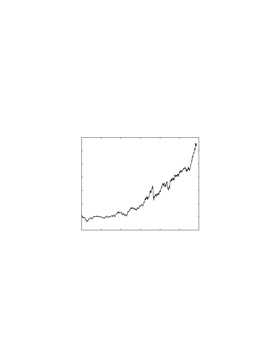
To get some logical output from such a calculation, the S&P500 index was detrended. The
plot of the index from 1972 through 1996 is shown in Fig. 1 below.

0

200

400

600

800

1000

1200

0

100

200

300

400

500

600

700

Data number

S&P 500 index

Fig. 1: S&P 500 index from 1972 through 1996

The trend is clearly exponential, which is logical since inflation cumulatively reduces the
value of the dollar. To detrend this data, the logarithm of this data was taken and this
logarithm of the index was detrended using detrend() in MATLAB, using a line
detrending, rather than simply removing the mean. Similarly, the long and short term
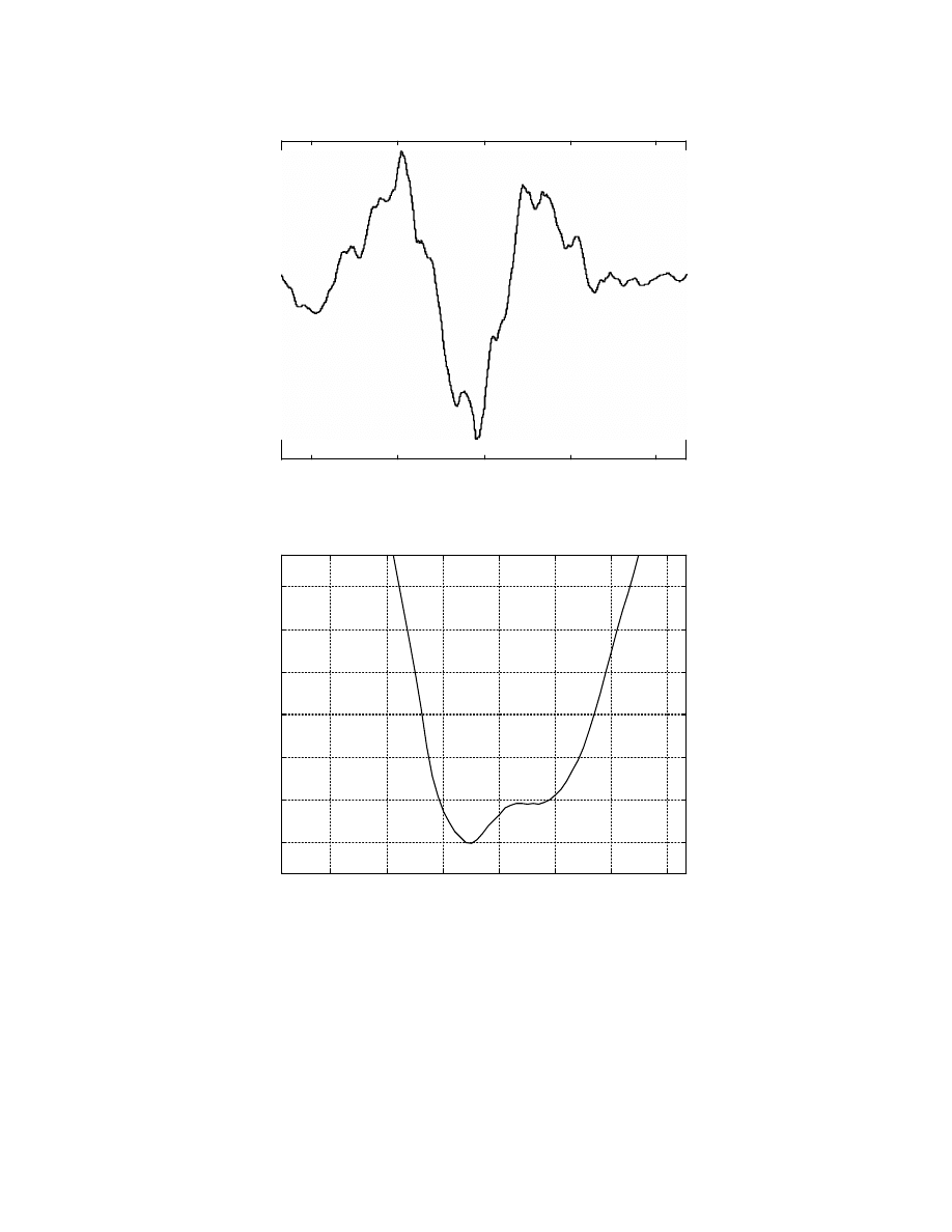
interest rates were detrended by simply removing the mean. Fig. 2 and 3 show the cross-
correlation between the long term interest rate delayed 53 weeks and the detrended index
(Fig. 3 is a zoomed in version of Fig. 2). It can be seen that there is a strong negative
correlation between the long term rate delayed 7 weeks through 25 weeks. Although, the
correlation with the lesser delay is stronger, here the long term rate delayed by 25 weeks is
used.

6

-1000

-500

0

500

1000

-0.6

-0.4

-0.2

0

0.2

0.4

Delay+53

Normalized cross-correlation

Fig. 2: Correlation - long term rate and index

-70

-60

-50

-40

-30

-20

-10

-0.62

-0.61

-0.6

-0.59

-0.58

-0.57

-0.56

Delay+53

Normalized cross-correlation

Fig. 3: Correlation - long term rate and index

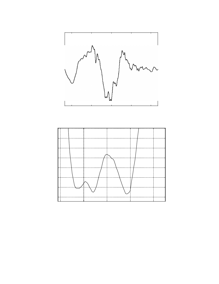
Similarly, Fig. 4 and 5 show the complete and zoomed in cross-correlation’s between the
short term interest rate and the index. From Fig. 4 and 5, it can be seen that there is a
strong negative cross-correlation between the short term rate and the index, with the short
term rate lagging the index either by 20 weeks or by 48 weeks. Since, both these inputs
are sufficiently delayed from the index, both are used as inputs to the neural network.

7

-1000

-500

0

500

1000

-0.5

0

0.5

Delay-53

Normalized cross-correlation

Fig. 4: Correlation - short term rate and index

-60

-40

-20

0

20

-0.43

-0.425

-0.42

-0.415

-0.41

-0.405

-0.4

-0.395

Delay-53

Normalized cross-correlation

Fig. 5: Correlation - short term rate and index

Feature extraction

Given, the above analysis the inputs to the neural network are:

•

The stock index value for the present week (all values are weekly closing values)

•

the weekly long term interest rate, delayed by 25 weeks,

•

the weekly short term interest rate, delayed by 20 weeks and

•

the weekly short term interest rate, delayed by 48 weeks.

8

The stock market future value also depends on the trend of the market as well as the trend
of the interest rates. To include this information, additional inputs are used. These are:

•

The difference between the present week’s index and that of the previous week

(referred to as the first difference). Since, this difference can be positive or negative, it
is encoded (as done in [7]) using two inputs. The first one is the absolute value of this
first difference and the second one is arbitrarily chosen as: 0.8 if the difference is
positive, 0.2 if the difference is negative and 0 if there is no change. This encoded
sign of the difference is hereafter referred as the trend. These two inputs along with the
present S&P500 index value make up the first 3 inputs of the network.

•

To reduce the effect of the noise present in the weekly stock market variation, the

average of the last 5 weekly closing values of the index and the average of the last 10
weekly closing values of the index, along with their absolute first differences and
trends are used. These constitute the next 6 inputs of the network.

•

To account for the long term interest rate, the long term interest rate delayed by 25

weeks and its absolute difference and trend are used as inputs 10 through 12. The
short term interest rate is accounted for by using the rate delayed by 48 weeks as well
as the rate delayed by 20 weeks along with their respective absolute differences and
trends, thus giving inputs 13 through 18.

The desired output of the network is the stock index value for the next week. Thus, the
neural network to be used has 18 inputs and 1 output. A simple feedforward network is
used with standard vanilla backpropagation training.

Normalization

The stock market index as seen from Fig. 1 has a continuously rising exponential trend. If
the index value is normalized linearly and fed to the neural network, it is possible that the
normalized future values of the index will be greater than unity, so that the neural network
will never be able to track those values. Hence, a non-linear normalization is required.
The function selected for normalization is the hyperbolic tangent function, as suggested in
[10]. The actual function used is:

spx_norm = 0.5*(1+tanh((spx-spx_avg)/A))

(1)

where, spx_norm is the normalized value and spx_avg is the average of the index over the
training data only. A is a constant to obtain the desired data range (so as to avoid
saturation of the tanh function. The tanh function will give an output in the range [-1,1],
which is then converted to [0,1] linearly (by adding 1 and then multiplying by 0.5).

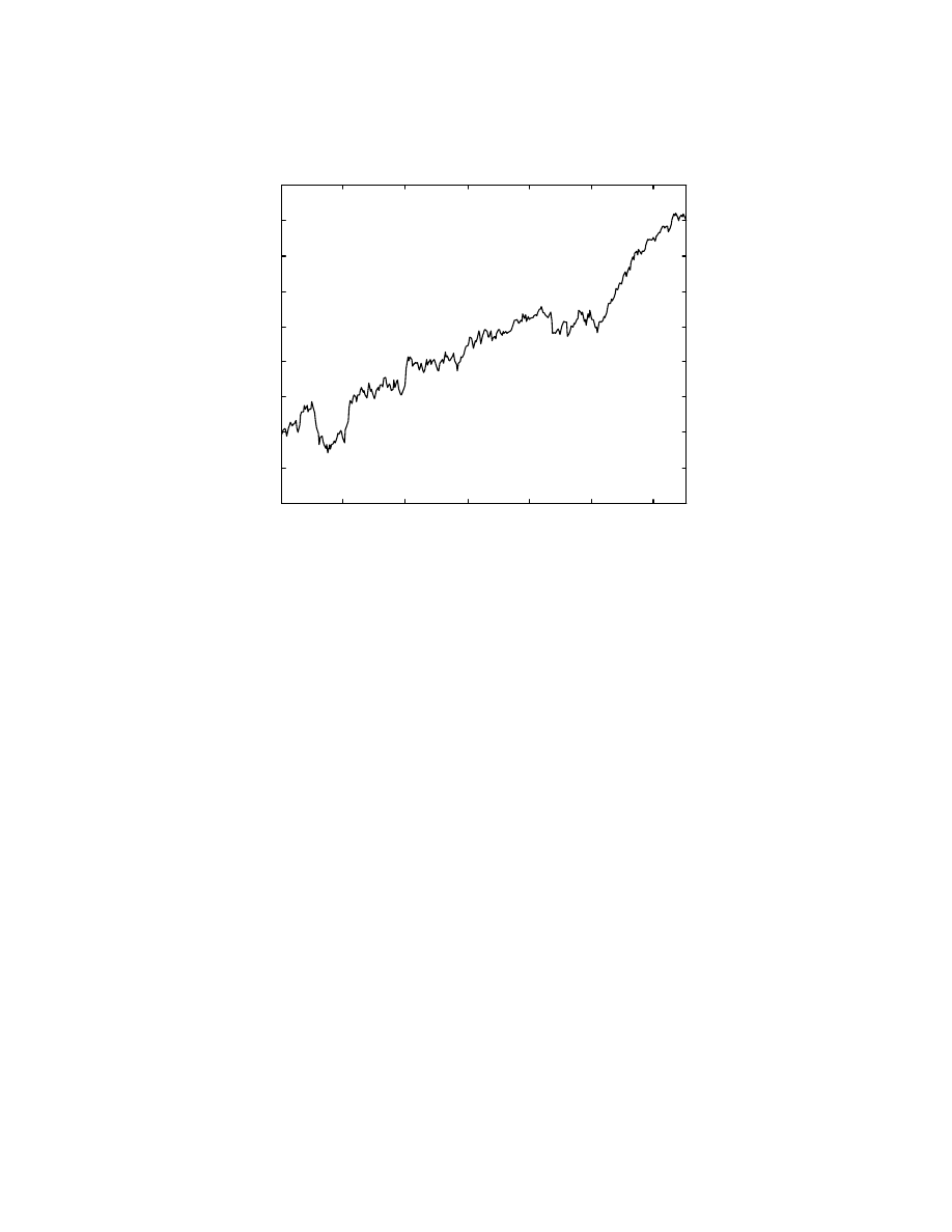
As a first try, such a normalization was used and the data selected was the last 325 weeks
(6 years) with the testing data being the last 50 weeks and the training based on 275
weeks before the testing data. As, seen from Fig. 1, the stock index is higher for the test
data than for the training data, so that the neural network never sees the desired values in
the range of the test data during training. This can be seen from Fig. 6, which shows the
normalized value for the training and testing data of the S&P500 index. In the first 275
data points, which constitutes the training set, the normalized index has a maximum value
of 0.7339, while in the test region the maximum value is 0.9211. Thus, the network cannot

9

be expected to learn the relationship and give the correct output and this was confirmed
after training and testing of the network using this kind of normalization.

50

100

150

200

250

300

0.1

0.2

0.3

0.4

0.5

0.6

0.7

0.8

0.9

Data number

Normalized S&P 500 index

Fig. 6: Normalized index in training and test regions

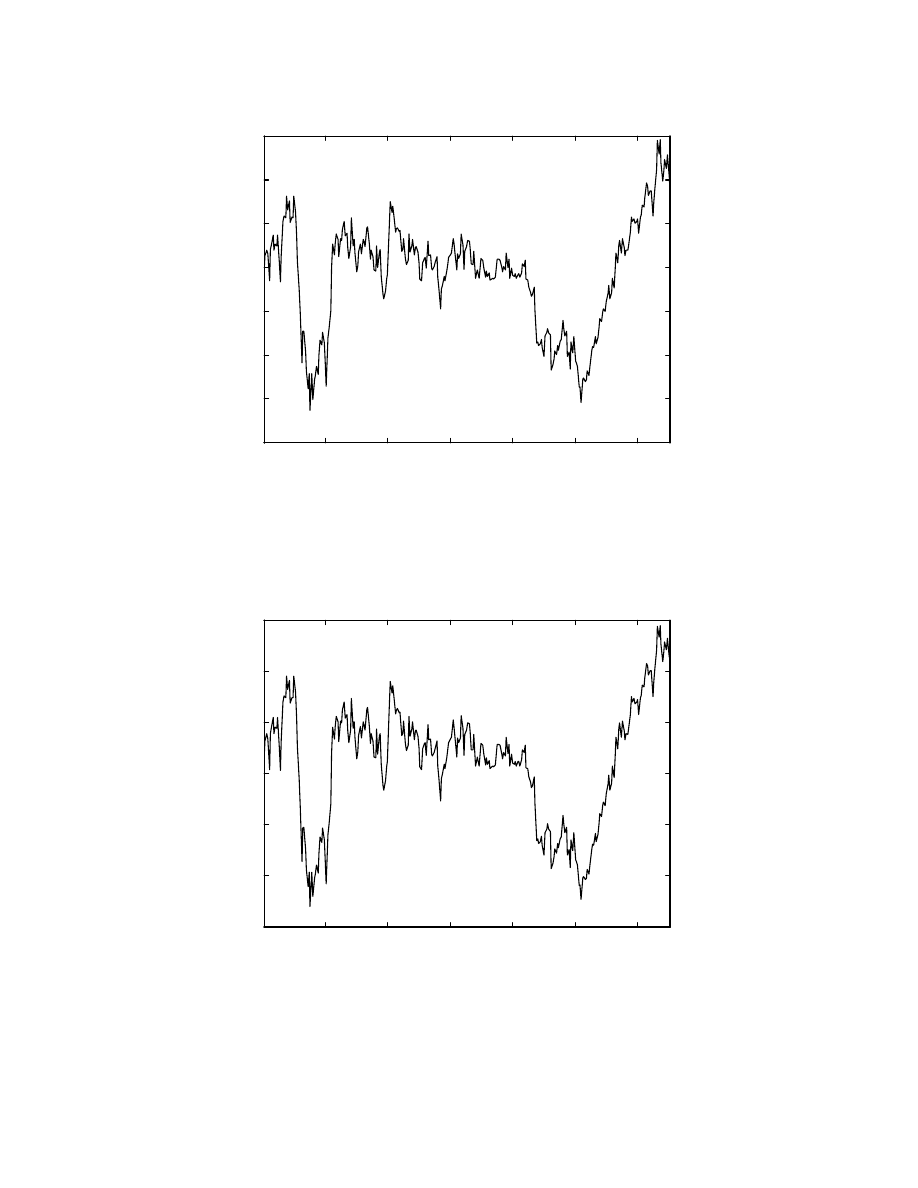
To remove this problem, the solution chosen was to detrend the data by taking the
logarithm of the S&P 500 index and then removing the linear trend from it. The
detrending was done by fitting a line (using polyfit() in MATLAB) to the training data
only and then removing this line from both the training and testing data. Fig. 7 shows the
detrended combined training and testing range of the S&P500 index using such an
approach. Although, the desired output is still higher at the end of the testing region, the
difference is much less than in Fig. 6.

10

50

100

150

200

250

300

-0.06

-0.04

-0.02

0

0.02

0.04

0.06

0.08

Data number

Detrended S&P 500 index

Fig. 7: Detrended index in training and test regions

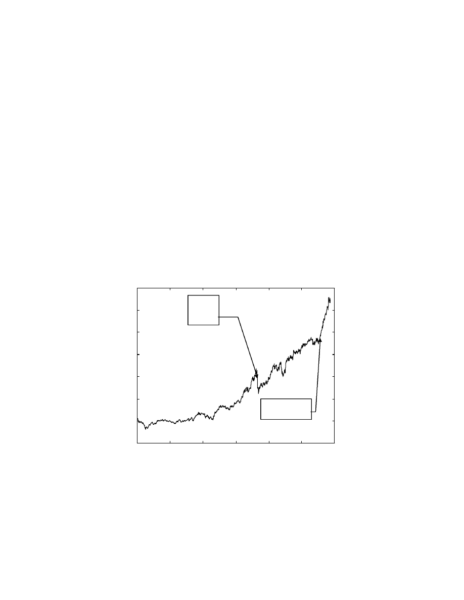
This detrended index is then used to obtain the 5-week and 10-week moving averages as
well as the first differences and the trends. The detrended index is then normalized using
equation (1), with A = 0.1 and this normalized detrended index is plotted in Fig. 8, below.

50

100

150

200

250

300

0.2

0.3

0.4

0.5

0.6

0.7

0.8

Data number

Normalized detrended index

Fig. 8: Normalized detrended S&P 500 index

Given this data, the network can be expected to learn the trend and give good results. The
5-week and 10-week averages of the detrended index as well as the absolute value of the
first difference of the detrended index and averages are all normalized using eq. (1), with

11

different values for A (A = 0.1 for the index and the averages and is = 0.02 for the
absolute value of the 3 first order differences).

The interest rates fluctuate about a certain value and there is no cumulative or time
integral effect on their behavior, hence, the interest rates are not detrended and these are
normalized using simple linear normalization. The same applies for the absolute difference
of the interest rates. All the trends

have a value of either 0.8, 0.2 or 0.0 and as such don’t

need further normalization. This completes the data normalization for the neural network.
The same techniques and constants are used for any other range of training and testing
data.

4. Test results

The neural network was trained using standard backpropagation for 2 different test cases,
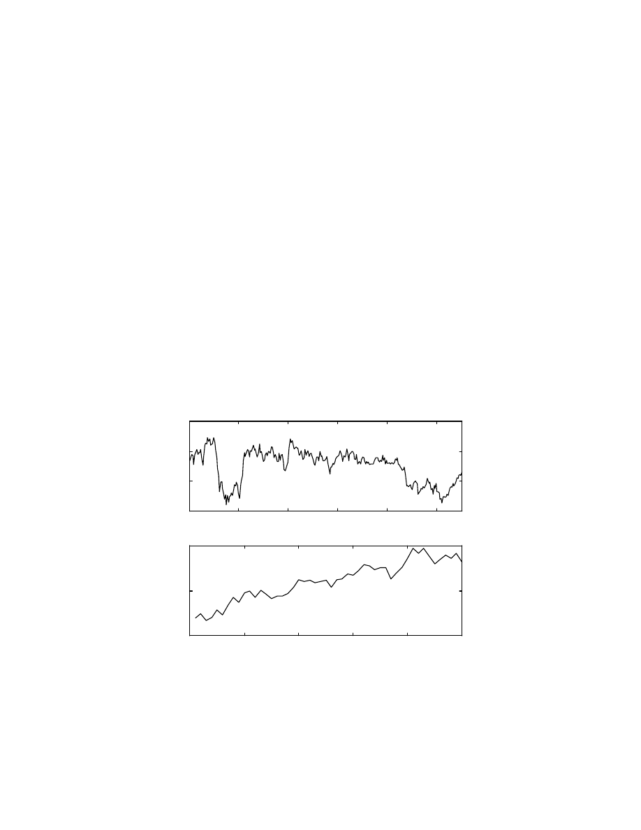
which are of critical interest from the point of view of desired performance. Fig. 1 shows
the variation of the S&P 500 index and is reproduced below for ready reference. It can be
seen that there is a big market crash around the 730

th

data point (October, 10

th

, 1986) and

there is a strong bull market beginning around the 1110

th

data point (January, 21

st

, 1994).

It would be interesting to see how the network performs for these worst case examples,
since, it would be expected to perform extremely well, when the training and testing data
is in the same range.

0

200

400

600

800

1000

1200

0

100

200

300

400

500

600

700

Data number

S&P 500 index

Fig. 1: S&P 500 index from 1972 through 1996

To test the network in these critical regions, it is trained using data from about 4 years
prior to the crash of 1986 or the start of the 1994 bull run. For both these test cases, the
network used has one hidden layer with 7 hidden neurons and 19 input neurons (input data
plus a unity input for the offset). Weights are initialized to random values in the range [-
1,1]. The hidden and output layers use a sigmoidal activation function. While the offset for
the hidden layer is provided by the fixed unity input of the 19

th

input neuron, there is no

Crash
October,
1986

Bull market
since, Jan 1994

12

offset for the sigmoids in the output layer. These test cases and the results obtained are
analyzed below.

Case 1: Bull run since Jan, 1994

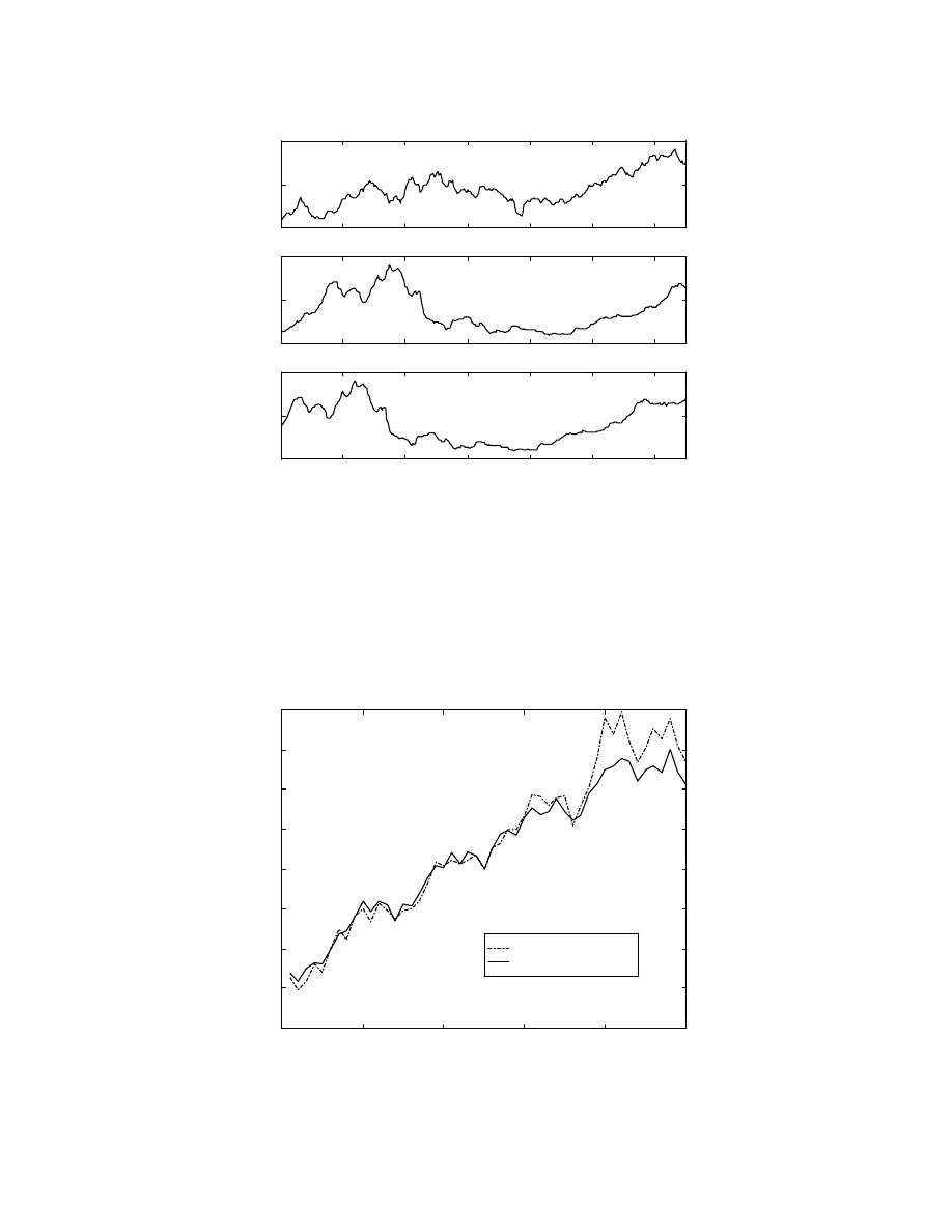
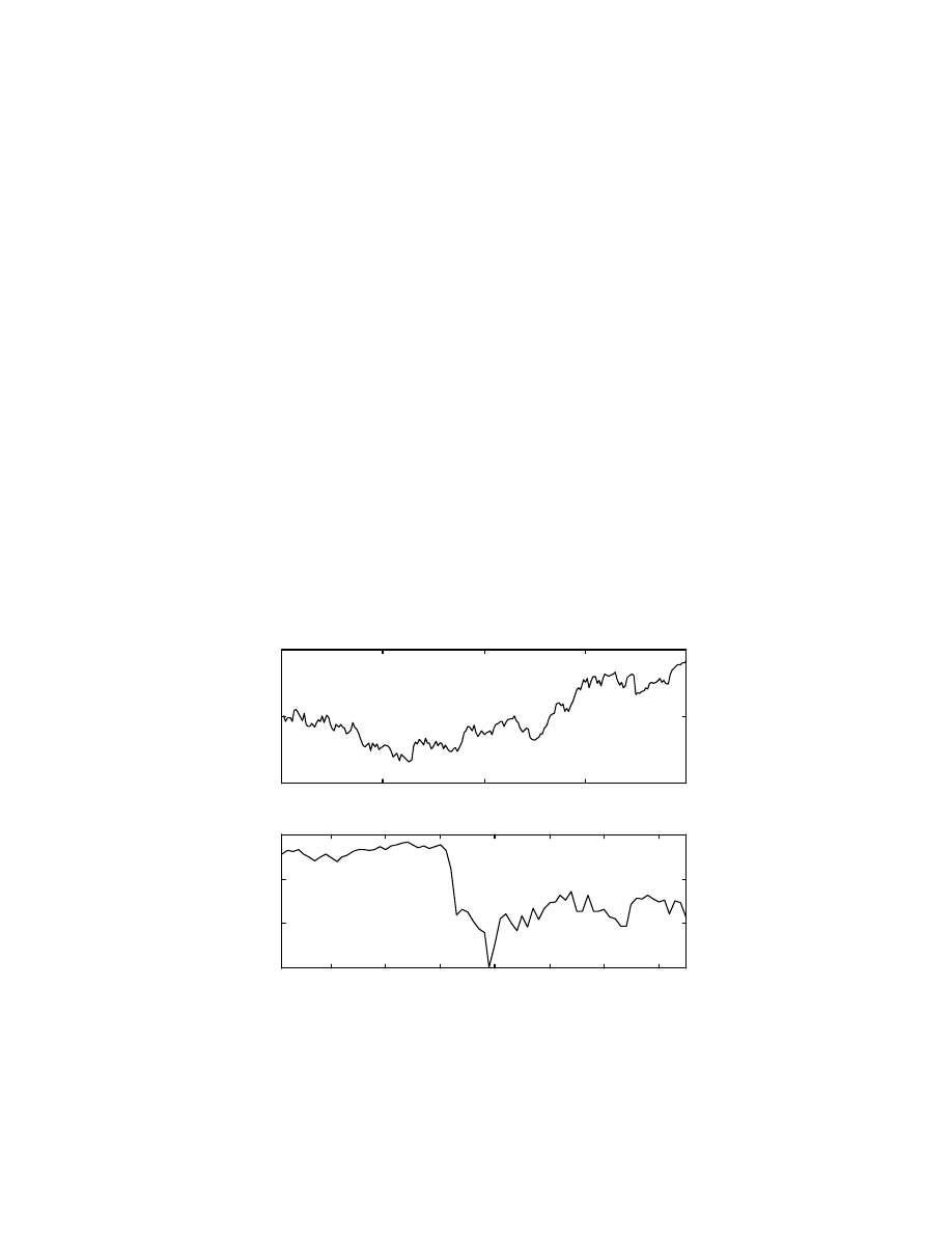
Fig. 9 shows the normalized training and test data of the S&P500 index, while Fig. 10
shows the normalized training and test data for the interest rates. The data starts from the
850

th

data point and the training data is of length 275 while the test data has a length of 50

weeks. It can be seen that the long term interest rate is rising for most part of the bull run
(testing data) except at the end, while the short term rate delayed by 20 weeks is rising
initially and then constant. This change from rising to constant is expected to have some
effect on the market. However, in this region the main effect is expected to come from the
market momentum itself, as analyzed by economists elsewhere [9].

Test results

Fig. 11 shows the test results for this case. The testing is done using the trained network
and the output for each week is compared with the desired output. It can be seen from the
figure that the network is able to predict the bull run consistently, one week in advance. It
predicts the correct trend of the stock index 43 times out of the test sample of 50 points.
The maximum percentage error expressed as a percentage of the desired output is only
4.044 %, while the average error is only 0.95%. Thus, the networks performs extremely
well and this performance can be suitably used to time the market.

50

100

150

200

250

0.2

0.4

0.6

0.8

Data number

Training data

Fig. 9: Training and testing data (S&P500 index)

0

10

20

30

40

50

0.4

0.6

0.8

Data number

Testing data

13

50

100

150

200

250

300

0

0.5

1

Short rate

48 week delay

50

100

150

200

250

300

0

0.5

1

Short rate

20 week delay

50

100

150

200

250

300

0

0.5

1

Long rate

Fig 10: Training and test data for interest rates

Even after detrending and normalization, which is based on training data only, the
desired output from the network is higher than the values it is trained on (Fig. 9). As such,
the network is able to predict an increase in the output even if it is not trained for the
exact values of the output range. This augurs well for a good performance in the future,
provided that care is taken to normalize the data so that a sudden increase in the index
value will not saturate the normalized value.

Desired value

Predicted value

0

10

20

30

40

50

500

520

540

560

580

600

620

640

660

Data number

S&P 500 index

Fig. 11: Predicted and desired S&P 500 index

Correct trend - 43 out of 50 times

Max. % error = 4.044%

Avg. % error = 0.95%

14

It can be argued that the network can be trained every week rather than keeping it based
on the training, which will be very old near the end of the 50

th

week. Moving the training

window every week and retraining the network is a valid approach, which might be
necessary in practice. However, there is a danger of the network training on the noise,
inherent in the weekly changes and hence, performing worse than this network. In any
case, this procedure can be modified suitably and the prediction window can also be
reduced to suit the requirements.

Case 2: Crash of October, 1986

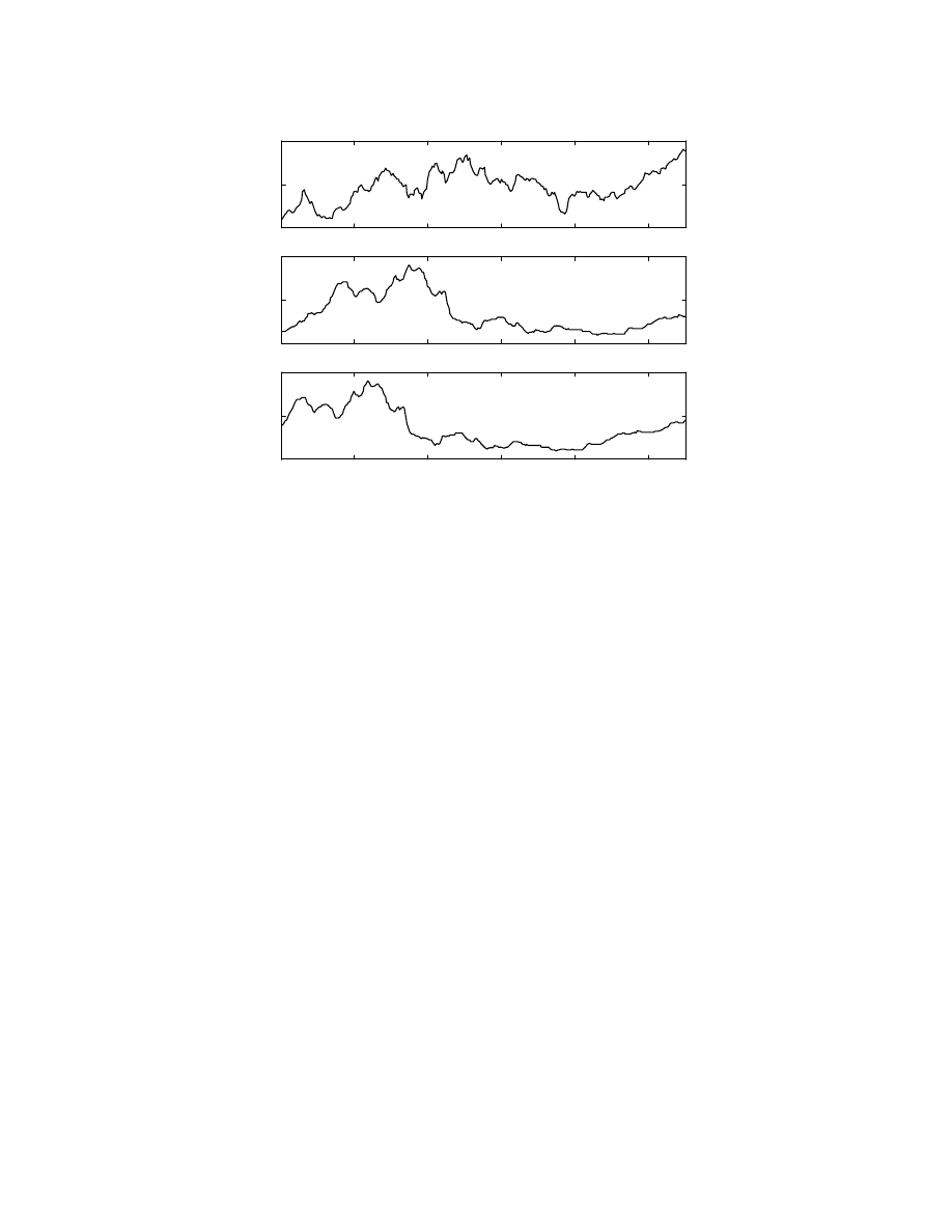
Fig. 12 on the shows the index values in the training and testing region for this second
case, where the training data starts from the 500

th

data point and is 200 data points long

while the test data extends over 75 weeks immediately following the training data and
includes the big crash. Fig. 13 shows the interest rates for the training and test regions
combined. In this case, the delayed long term interest rate is falling in the training phase
when the S&P 500 index has a rising trend, while during the testing phase it is rising very
fast, when the index is falling. The short-term rate delayed by 20 weeks is also increasing,
albeit rather slowly, in the test period. Thus, in this test case, it is expected that the effect
of rising interest rates will predict the crash. There is not much sustained momentum in the
training data of the index, since it is rising and falling or in other words, the change in
index is oscillating between positive and negative values. The network having 7 neurons in
the hidden layer is trained for 900 iterations, with a constant step size of 0.4 and the test
results are detailed in the next section.

0

50

100

150

200

0

0.5

1

Data number

Training data

Fig. 12: Training and testing data (S&P500 index)

10

20

30

40

50

60

70

0.4

0.6

0.8

1

Data number

Testing data

15

50

100

150

200

250

0

0.5

1

Long rate

Fig 13: Training and test data for interest rates

50

100

150

200

250

0

0.5

1

Short rate

48 week delay

50

100

150

200

250

0

0.5

1

Short rate

20 week delay

Test results

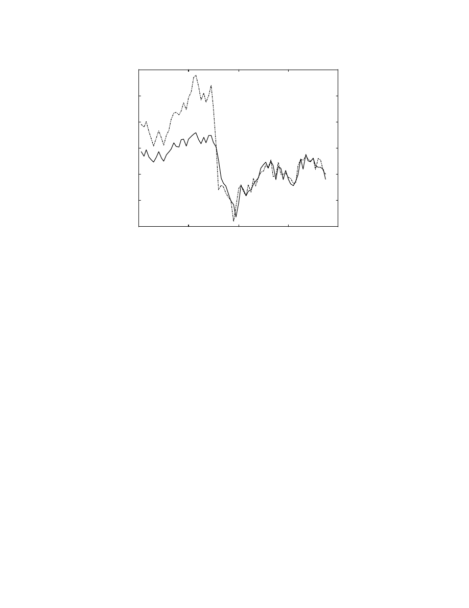
Fig. 14 shows the test results for this case. The plot shows that the network is able to
predict the severe crash one-week before it occurred. Although, the network output is
lower than the actual values in the initial part of the test range, there is no trend in the
stock index, which would force the network to predict a crash. Thus, a network using only
the past index values would have been unable to predict this crash, which can be attributed
to the rising long term interest rates. For this case, the network predicts the correct trend
of the stock index 65 times out of the test sample of 75 points. The maximum percentage
error expressed as a percentage of the desired output is much higher than case 1 and is
13.17 %, while the average error is only 4.18%. The main source of the error is that the
network doesn’t predict the initial rise in the market very well, in terms of the index level.
This is in fact conservative since, any other model which would have predicted the initial
high rise correctly might have given an incorrect and premature buy signal immediately
followed by a sell signal. Such rapid changes are not desirable since the number of trades
is increased along with the associated transaction costs.

16

0

20

40

60

80

220

240

260

280

300

320

340

Data number

S&P 500 index

Fig. 14: Predicted and desired S&P 500 index

Max. % error = 13.17%

Avg. % error = 4.18%

Correct trend - 65 out of 75 times

This concludes the presentation of the test results for both the cases. The next section
presents the conclusions and possibilities of future work based on this project.

5. Conclusions and Future work

The following conclusions can be drawn from this project work:

•

A feedforward neural network has been successfully applied to the problem of a one-

week ahead prediction of the weekly closing prices of the S&P 500 index.

•

The dependence of the stock index on interest rates is established using cross-

correlation values and the inclusion of this dependence is seen by the performance of
the network for the second test case.

•

The trained neural network performs very well even for worst cases where there are

sudden rises or falls in the stock market index.

Future work

The original aim of this project was the application of the available data for medium term
prediction of the stock market index using some form of a recurrent network.

•

For medium term prediction, the method used in [10] and described in Section 2, can

be applied. There, the network predicts the stock value for the next few weeks and the
training for that is performed by feeding the error for outputs back as inputs during
training.

•

A recurrent network such as an Elman net can be applied so that the effect of the

interest rates on the stock index prior to the data used can also be accounted for.
Thus, a history or integral effect can be obtained using a recurrent network.

•

Even if a recurrent network is used, some delay will have to be assumed for using the

interest rates. The easiest case would be to use current interest rates without any delay

17

and allow the training to establish the actual delay. There is a lot of scope for work
with regard to the choice of the delay in the interest rates.

•

For using this technique in practice, a trading mechanism based on the predictions of

the network needs to be established which will give buy/sell signals and will maximize
profit without increasing the number of trades by a large number.

6. References

[1] Black, F. and Scholes, M., “The pricing of Options and Corporate Liabilities,” Journal of

Political Economy, vol. 81, no. 3, May-June 1973.

[2] Azoff, E. M., Neural network time series forecasting of financial markets, Wiley, New York,

1994.

[3] Connor, J. T., Time Series and Neural Network Modeling, Ph.D. thesis, University of

Washington, Seattle, 1993.

[4] White, H., “Economic prediction using neural networks: The case of IBM daily stock

returns,” IEEE International Conference on Neural networks, vol. 2, pp. 451-458, San
Diego, 1988.

[5] Chenoweth, T., Obradovic, Z. and Lee, S., “Technical trading rules as a prior knowledge to a

neural networks prediction system for the S&P 500 index,” Northcon/95, pp. 111-115,
Portland, Oct. 1995.

[6] Gia Shuh Jang et al, “An intelligent stock portfolio management system based on short-term

trend prediction using dual-module neural networks,”. Proc. of the 1991 International
Conference on Artificial Neural Networks, vol. 1, pp. 447- 52, Finland, June 1991.

[7] Freisleben, B., “Stock market prediction with backpropagation networks,” 5th Intl. Conf. on

the Industrial and Engineering Applications of Artificial Intelligence and Expert Systems,
pp. 451-60, Germany, June 1992.

[8] Komo, D, Chang, C. I. And Ko, H., “Stock market index prediction using neural networks,”

Applications of Artificial Neural Networks V, pp. 516-26, Orlando, April 1994.

[9] Zweig, M. E., Martin Zweig's winning on Wall Street, Warner Books, New York, 1986.
[10] Matsuba, I., “Neural sequential associator and its application to stock price prediction,” Proc.

IECON ‘91, vol. 2, pp. 1476-9, Japan, Nov. 1991.

[11] Kamijo, K. and Tanigawa, T., “Stock price pattern recognition - a recurrent neural network

approach,” Proc. IJCNN 1990, vol. 1, pp. 215-21, San Diego, June 1990.

[12] Kimoto, T. and Asakawa, K., “Stock market prediction system with modular neural

networks,” Proc. IJCNN 1990, vol. 1, pp. 1-6, San Diego, June 1990.